1

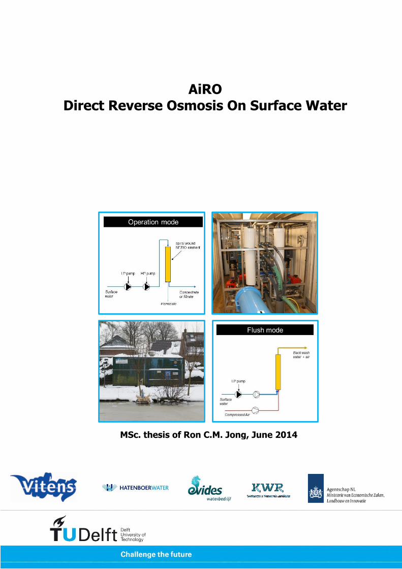
AiRO Direct Reverse Osmosis On Surface Water

MSc. thesis of Ron C.M. Jong, June 2014

2

3

AiRO: Direct Reverse Osmosis On Surface Water Semi practical scale pilot research at Vitens location Montfoort

Ronaldus Cornelius Maria Jong

for the degree of:

Master of Science in Civil Engineering

Date of submission: 6th of June 2014 Date of defense: 20th of June 2014

Committee: Prof. dr.ir. W.G.J van der Meer Delft University of Technology Sanitary Engineering Section Prof.dr.ir T.N. Olsthoorn Delft University of Technology Water Resources Section Dr.ir. J.Q.J.C. Verberk Evides Watercompany Dr.ir. S.G.J. Heijman Delft University of Technology

Sanitary Engineering Section Ir. A.H. Haidari Delft University of Technology

Sanitary Engineering Section

Sanitary Engineering Section, Department of Water Management Faculty of Civil Engineering and Geosciences Delft University of Technology, Delft

4

5

Abstract Surface water is microbiological unsafe, contains too much salts and is polluted with anthropogenic substances like pesticides, medicines, endocrine disruptors and industrial chemicals. The production of safe drinking water out of this water is only possible by applying a robust treatment. A process that can remove virtually all unwanted substances from the water in one step is reverse osmosis (RO). The main bottleneck in the wider application of RO with spiral wound membranes is the membrane fouling. This occurs on the feed spacer of the spiral wound membranes and at the membrane surface. This fouling occurs with particles, salts and/or microorganisms and results in a raise in pressure drop and reduction in permeate quality. An innovative idea to deal with above mentioned drawbacks is a membrane process in which spiral wounded NF/RO membrane elements are cleaned hydraulic (mechanically). The membrane is placed vertical and the membrane fouling is controlled by means of a periodic air/water flush, AiRO called (combination of the words air and RO). This AiRO process line needs hardly any pretreatment, is free of antiscalant dosage, uses less chemicals than traditional NF/RO and the concentrate is easy to dispose to surface water. The semi practical AiRO research described in this thesis is carried out with an automated pilot plant that was equipped with 2 8” RO membranes. The pilot was placed at the banks of the Hollandse IJssel river in Montfoort. The pre treatment was a drum filter. The pilot was started up in December 2010 and operated non stop for one and a half year. The research has shown that AiRO is a reliable robust barrier in a surface water purification process line. There is no effect on the operation of the process if the turbidity of the feed water varies between 4 and 75 FTU and if the oxygen content in the feed water varies (indication for microbiology). The process appeared to be economic interesting and withstood the practical durability test. Pre treatment of the feed water of the AiRO with a 120 µm micro strainer is sufficient. The commonly in Netherland applied 35 µm micro strainer is advised because it will give advantages for the AiRO process (less wear in pumps and energy recovery) and will promote the surge for a solution for the concentrate. Commercial available NF/RO elements are applicable in AiRO and the membrane stack is composed with pressure vessels with 2 8” elements in series. The investment costs of a complete drinking water treatment with the AiRO process are 20 to 33% lower than a treatment based on UF and RO. The application of 16” pressure vessels containing 2 16” elements in series may result in even lower investment costs. A flush was executed with the maximum allowed feed pressure (specs. Membrane manufacturer), the flush water velocity was 0,2 m/s in the membrane feed spacer, and with an air velocity of 0.24 Nm/s. Energy recovery from concentrate (Fedco) is essential to obtain energy efficiency. The flush program that resulted in a stable operation of the process consists of the steps:

Flush step Duration [ s ]

Water velocity [ m/s ]

Air velocity [ Nm/s ]

Preflush Combined flush Postflush

Adjustable1 120

Adjustable2

0.2 0.14 0.2

- 0.24

- 1 achievement of stable water flow 2 remove air from feed spacer and pressure vessel

The flush interval is 4 hours and pressure drop NPD is the parameter for fine tuning of the interval duration. A flush should start if the NPD doesn’t rise linear anymore. A CIP has to take place, if the NPD before a flush rises above 50 kPa. The applied chemicals have to be balanced on the feed water composition. Manganese oxides by example are hardly washed out by a flush, they have to be removed during a CIP with citric or ascorbic acid.

6

The design recovery is 35% and operation of AiRO at this low recovery results in a large concentrate stream, which is free of antiscalant and with a low content of salts. This flow is expected to be allowed to discharge to surface water. The flush water can be discharged to surface water, after sedimentation of the solids in it. The produced sludge is free of chemical additions. This will improve the useful application of the sludge. The used CIP fluid has to be discharged to the sewer after neutralisation of the pH.

7

Preface This research was conducted as my Master Thesis project for the graduation from the Sanitary Engineering Section, Water Management Department of the Faculty of Civil Engineering and Geoscience of the Delft University of Technology, the Netherlands. Topic of this Master Thesis is AiRO, a novel membrane technology for treating surface water. In this type of RO, the elements are placed vertically, the operation is downflow and every 4 hours the element is upflow flushed with water and air to remove fouling. The pilot at the banks of the Hollandse IJssel river in Montfoort, was started up in December 2010. The pre treatment was a drum filter and the pilot operated non stop for one and a half year. In this thesis are the results and conclusions of this semi practical scale research described. The first period of the research is carried out under the wings of the AiRO Innowator project that ended at the end of 2011 and was state-aided by AgentschapNl. Partners were Evides (Sjack van Agtmaal and Martin Pot), KWR (Emile Cornelissen and Erwin Beerendonk), Hatenboer Water (Carel Averink and Jan Arie de Ruijter) and Vitens (Wilbert van de Ven and Ron Jong). The project was continued, supervised by a TU Delft (members of the Assessment Committee), Hatenboer-Water (Jan Arie de Ruijter) and Vitens (Ron Jong) project team, financial supported by the Vitens Business Development department. My appreciation goes to the contribution to the AiRO project of the members of both project teams. The Master is followed as mid-career course, introduced by emeritus professor Hans van Dijk. I’m Vitens grateful for the opportunity they have given to me to follow this course. The six years that the part-time course took, are experienced as an instructive and educational period. Not only concerning content but especially the interaction and discussions with (international) students were fruitful. On the other hand it was challenging to keep the balance between family life, study, Vitens and free time. For this reason I especially want to thank my wife Antoinette and my daughters Iris and Amber for the understanding they showed in periods that I was too grumpy (the days before an exam were the bottom…). Fellow part-time students Bas Rietman and Frank Schoonenberg and student Gea Terhorst were a good outlet, to place the study in its proper perspective. Thank you for that. I would like to express my gratitude to members of the Assessment Committee, Amir Haidari, Jasper Verberk, Bas Heijman and most of all my supervisor, professor Walter van der Meer, for their patience and professional feed back during my research. I want to thank Amir for the time consuming detail check of the text. Further, I would like to thank my colleague Ferrie den Uijl for the crucial assistance during the construction, operation and cleaning (CIP) of the pilot at Montfoort and Patrick Teunissen and Gerrit Jan Zweere for their support during the research. I hope you are now curious to the content of this report, enjoy reading it.

8

Content Preface 7 Content 8 List of abbreviations 10 1 Introduction 11

1.1 Membrane filtration 11 1.2 Membrane element 12 1.3 Fouling 13 1.4 Membrane fouling types 13 1.4.1 Particulate Fouling 13 1.4.2 Scaling (inorganic fouling) 14 1.4.3 Organic fouling 14 1.4.4 Biofouling 14 1.5 Biofouling managing systems 15 1.6 Principle of AiRO 15 1.7 Literature review 17 1.8 Objectives 27 1.9 Outline 28

2 Materials and methods 29 2.1 Research location Montfoort 29 2.2 Raw water intake 30 2.3 Pretreatment: Drum filter 30 2.4 AiRO unit 31 2.4.1 Operation mode 32 2.4.2 Air water flush mode 32 2.4.3 CIP (Clean In Place) 33 2.4.4 Applied membranes 34 2.4.5 Settings of pilot 34 2.5 Measuring instruments 35 2.6 Sample programme 36 2.7 The MFS 36

3 Results 38 3.1 Overview of results of pilot research Montfoort 38 3.1.1 Applied pretreatment during AiRO research 38 3.1.2 Steps of flush of the AiRO process? 39 3.2 What will be the duration of the defined flush steps? 39 3.2.1 Duration of the preflush 40 3.2.2 Duration of the postflush 40 3.2.3 Duration of the air/water flush 40 3.3 What is the preferable time interval between flushes? 42 3.4 What will be the water and air velocity during flush? 44 3.4.1 Determination of intensity of flush steps 44 3.4.2 Determination of influence of intensity of flush steps 49 3.5 Does the feed water quality influence the AiRO process? 50 3.5.1 Effect of particles in feed water 51 3.5.2 Biology in feed water; low oxygen 54 3.6 Which CIP procedure is preferred and when will it take place? 57 3.6.1 Effect of CIP procedure on MTC 57 3.6.2 Removed substances 58 3.6.3 Effect of CIP on NPD 60 3.6.4 What is maximum acceptable NPD? 62 3.7 What is the design of a treatment with AiRO and what does it cost? 64 3.7.1 What will an AiRO stack design look like? 65 3.7.2 Introduction of 2 element pressure vessel 66 3.7.3 Design of an AiRO stack with 2 element pressure vessels 67

9

3.7.4 Economical aspects 68 3.8 Summarized results 71

4 Discussion 73 4.1 Preferable pre treatment 73 4.2 The preflush can be shorter 73 4.3 Accuracy of economic calculations 73 4.4 Better distribution of flush air 74 4.5 Variabel flush interval 74 4.6 Applicable pressure vessels 74 4.7 Operational aspects of a 2 element pressure vessel 75

5 Conclusions and recommendations 76 5.1 Conclusions 76 5.2 Recommendations 77

List of references 78 Annex 1 Overview of applied equations 81

Calculation of recovery and flux 81 Normalization of results 81

Annex 2 Pictures of construction of AiRO pilot at location Montfoort 84 Annex 3 AiRO pilot construction drawings 85 Annex 4 Specs of applied membranes 87 Annex 5 MTC, NPD and NSP during AiRO research 89 Annex 6 Water quality of Hollandse IJssel river 91 Annex 7 Hydraulic calculations of AiRO stack design 94 Annex 8 Set up of investment costs and substantiating of costs 96 CV of the author 98

10

List of abbreviations

AiRO air flushed reverse osmosis AOC easy assimilable organic carbon AWC air/water cleaning BAC biological granular activated carbon CIP cleaning in place, chemical cleaning of membranes DAF dissolved air flotation EC electrical conductivity of water (µS/cm) EPS extracellular polymeric substances FTU formazin turbidity unit GAC granular activated carbon HP pump high pressure pump, feed pump of NF/RO KWR Kiwa Water Research and technology LP pump low pressure pump, flush pump AND feed pump of HP pump NC135 NovoClean 135, alkaline cleaning, Novochem Water Treatment BV NC136 NovoClean 136, acid cleaning, Novochem Water Treatment BV MF microfiltration MFS membrane fouling simulator MTC mass transfer coefficient (m/s Pa) NF nanofiltration NOM natural organic matter NPD normalized pressure drop (kPa) NSP normalized salt passage (% of EC) OSMF One Step Membrane Filtration PIV Particle Image Velocimetry ppm part per million QG gas flow rate (Nm3/h) QL liquid flow rate (m3/h) R retention (%) RO reverse osmosis TMP trans-membrane pressure (kPa) UF ultrafiltration v velocity (m/s) WTP water treatment plant WMO Waterleiding Maatschappij Overijssel, drinking water supply company WWTP waste water treatment plant

11

1 Introduction

Membrane technology based water treatment systems gained considerable interests in the past decades due to the ability to remove a large number of compounds in a single purification step. It can contribute considerably to the availability of pure and healthy freshwater for personal and industrial use. Membrane systems are designed to remove a wide variety of substances (pathogens, toxic compounds, salts, humic acids, metals, etc.) from e.g. groundwater and (fresh and sea) surface water. Reuse of industrial and municipal wastewater becomes feasible if membranes are used in the purification process. However, all membrane systems eventually foul during operation and need to be cleaned regularly. Among the different types of fouling, biofouling is the most persistent and difficult type to control (Flemming, 1997). Biofouling in a water system results in the significant reduction of water quality and the amount of produced water (Bereschenko, 2010) due to growth of microorganisms on available surfaces. If biofouling is left unattended or if it is treated strongly with cleaning chemicals, the system performance and the lifetime of the membranes will be reduced (Patching, 2003).

1.1 Membrane filtration

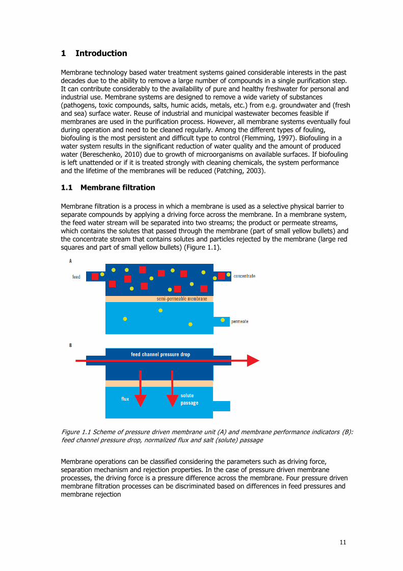
Membrane filtration is a process in which a membrane is used as a selective physical barrier to separate compounds by applying a driving force across the membrane. In a membrane system, the feed water stream will be separated into two streams; the product or permeate streams, which contains the solutes that passed through the membrane (part of small yellow bullets) and the concentrate stream that contains solutes and particles rejected by the membrane (large red squares and part of small yellow bullets) (Figure 1.1).

Membrane operations can be classified considering the parameters such as driving force, separation mechanism and rejection properties. In the case of pressure driven membrane processes, the driving force is a pressure difference across the membrane. Four pressure driven membrane filtration processes can be discriminated based on differences in feed pressures and membrane rejection

Figure 1.1 Scheme of pressure driven membrane unit (A) and membrane performance indicators (B):

feed channel pressure drop, normalized flux and salt (solute) passage

12

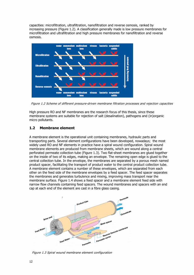
capacities: microfiltration, ultrafiltration, nanofiltration and reverse osmosis, ranked by increasing pressure (Figure 1.2). A classification generally made is low pressure membranes for microfiltration and ultrafiltration and high pressure membranes for nanofiltration and reverse osmosis.

High pressure RO and NF membranes are the research focus of this thesis, since these membrane systems are suitable for rejection of salt (desalination), pathogens and (in)organic micro pollutants.

1.2 Membrane element

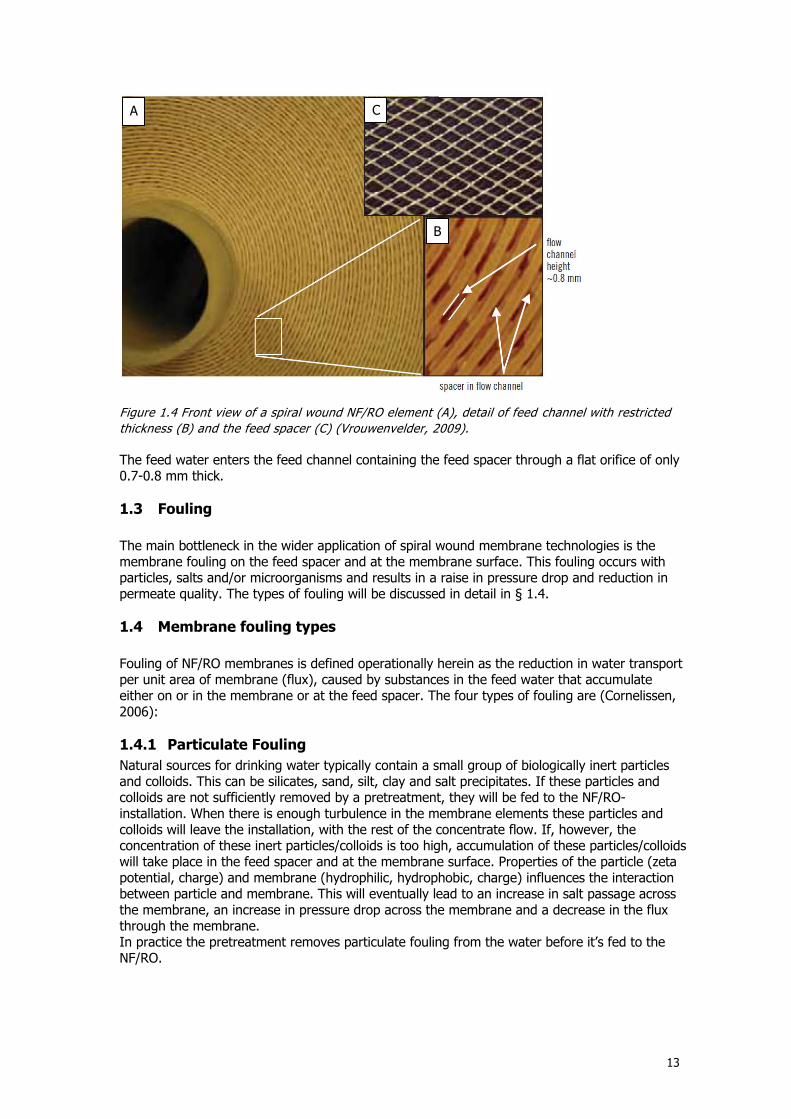
A membrane element is the operational unit containing membranes, hydraulic parts and transporting parts. Several element configurations have been developed, nowadays; the most widely used RO and NF elements in practice have a spiral wound configuration. Spiral wound membrane elements are produced from membrane sheets, which are wound along a central perforated permeate collection tube (Figure 1.3). Two flat-sheet membranes are glued together on the inside of two of its edges, making an envelope. The remaining open edge is glued to the central collection tube. In the envelope, the membranes are separated by a porous mesh named product spacer, facilitating the transport of product water to the central product collection tube. A membrane element contains a number of these envelopes, which are separated from each other on the feed side of the membrane envelopes by a feed spacer. The feed spacer separates the membranes and generates turbulence and mixing, improving mass transport near the membrane surface. Figure 1.4 shows a feed spacer and a membrane element feed side with narrow flow channels containing feed spacers. The wound membranes and spacers with an end cap at each end of the element are cast in a fibre glass casing.

Figure 1.2 Scheme of different pressure-driven membrane filtration processes and rejection capacities

Figure 1.3 Spiral wound membrane element configuration

13

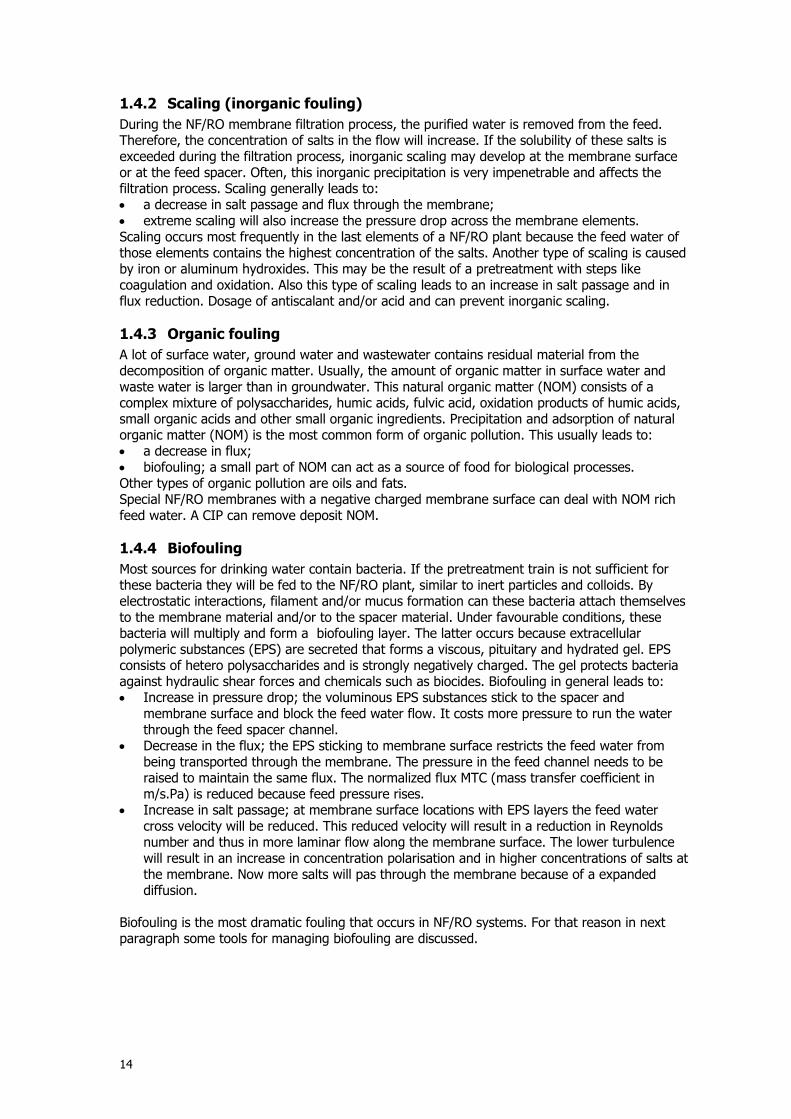
Figure 1.4 Front view of a spiral wound NF/RO element (A), detail of feed channel with restricted

thickness (B) and the feed spacer (C) (Vrouwenvelder, 2009).

The feed water enters the feed channel containing the feed spacer through a flat orifice of only 0.7-0.8 mm thick.

1.3 Fouling

The main bottleneck in the wider application of spiral wound membrane technologies is the membrane fouling on the feed spacer and at the membrane surface. This fouling occurs with particles, salts and/or microorganisms and results in a raise in pressure drop and reduction in permeate quality. The types of fouling will be discussed in detail in § 1.4.

1.4 Membrane fouling types

Fouling of NF/RO membranes is defined operationally herein as the reduction in water transport per unit area of membrane (flux), caused by substances in the feed water that accumulate either on or in the membrane or at the feed spacer. The four types of fouling are (Cornelissen, 2006):

1.4.1 Particulate Fouling

Natural sources for drinking water typically contain a small group of biologically inert particles and colloids. This can be silicates, sand, silt, clay and salt precipitates. If these particles and colloids are not sufficiently removed by a pretreatment, they will be fed to the NF/RO-installation. When there is enough turbulence in the membrane elements these particles and colloids will leave the installation, with the rest of the concentrate flow. If, however, the concentration of these inert particles/colloids is too high, accumulation of these particles/colloids will take place in the feed spacer and at the membrane surface. Properties of the particle (zeta potential, charge) and membrane (hydrophilic, hydrophobic, charge) influences the interaction between particle and membrane. This will eventually lead to an increase in salt passage across the membrane, an increase in pressure drop across the membrane and a decrease in the flux through the membrane. In practice the pretreatment removes particulate fouling from the water before it’s fed to the NF/RO.

A C

B

14

1.4.2 Scaling (inorganic fouling)

During the NF/RO membrane filtration process, the purified water is removed from the feed. Therefore, the concentration of salts in the flow will increase. If the solubility of these salts is exceeded during the filtration process, inorganic scaling may develop at the membrane surface or at the feed spacer. Often, this inorganic precipitation is very impenetrable and affects the filtration process. Scaling generally leads to: a decrease in salt passage and flux through the membrane; extreme scaling will also increase the pressure drop across the membrane elements. Scaling occurs most frequently in the last elements of a NF/RO plant because the feed water of those elements contains the highest concentration of the salts. Another type of scaling is caused by iron or aluminum hydroxides. This may be the result of a pretreatment with steps like coagulation and oxidation. Also this type of scaling leads to an increase in salt passage and in flux reduction. Dosage of antiscalant and/or acid and can prevent inorganic scaling.

1.4.3 Organic fouling

A lot of surface water, ground water and wastewater contains residual material from the decomposition of organic matter. Usually, the amount of organic matter in surface water and waste water is larger than in groundwater. This natural organic matter (NOM) consists of a complex mixture of polysaccharides, humic acids, fulvic acid, oxidation products of humic acids, small organic acids and other small organic ingredients. Precipitation and adsorption of natural organic matter (NOM) is the most common form of organic pollution. This usually leads to: a decrease in flux; biofouling; a small part of NOM can act as a source of food for biological processes. Other types of organic pollution are oils and fats. Special NF/RO membranes with a negative charged membrane surface can deal with NOM rich feed water. A CIP can remove deposit NOM.

1.4.4 Biofouling

Most sources for drinking water contain bacteria. If the pretreatment train is not sufficient for these bacteria they will be fed to the NF/RO plant, similar to inert particles and colloids. By electrostatic interactions, filament and/or mucus formation can these bacteria attach themselves to the membrane material and/or to the spacer material. Under favourable conditions, these bacteria will multiply and form a biofouling layer. The latter occurs because extracellular polymeric substances (EPS) are secreted that forms a viscous, pituitary and hydrated gel. EPS consists of hetero polysaccharides and is strongly negatively charged. The gel protects bacteria against hydraulic shear forces and chemicals such as biocides. Biofouling in general leads to: Increase in pressure drop; the voluminous EPS substances stick to the spacer and

membrane surface and block the feed water flow. It costs more pressure to run the water through the feed spacer channel.

Decrease in the flux; the EPS sticking to membrane surface restricts the feed water from being transported through the membrane. The pressure in the feed channel needs to be raised to maintain the same flux. The normalized flux MTC (mass transfer coefficient in m/s.Pa) is reduced because feed pressure rises.

Increase in salt passage; at membrane surface locations with EPS layers the feed water cross velocity will be reduced. This reduced velocity will result in a reduction in Reynolds number and thus in more laminar flow along the membrane surface. The lower turbulence will result in an increase in concentration polarisation and in higher concentrations of salts at the membrane. Now more salts will pas through the membrane because of a expanded diffusion.

Biofouling is the most dramatic fouling that occurs in NF/RO systems. For that reason in next paragraph some tools for managing biofouling are discussed.

15

1.5 Biofouling managing systems

Preventing Biofouling in a membrane filtration is not possible, it will always occur. Managing of biofouling is the only manner of dealing with this problem. Some of the practical methods of dealing with biofouling of surface water are: 1. Low fouling membranes 2. Application of biocides 3. Clean Operator Too (COTOO) 4. AiRO Low fouling membranes Most membrane manufacturers have low fouling membranes in their membrane line, some examples are: Hydranautics' LFC (Low Fouling Composite) is designed with a thicker brine spacer lowering

the NPD and requires less frequent cleanings while maintaining a high permeate flow. According to Hydranautics LFC elements combine neutral surface charge and hydrophilicity, providing significant reduction in fouling rates and increasing membrane efficiency by restoring nominal performance after cleaning;

Torays’ Less Fouling RO Membrane has extremely less bacteria attachment and prevents bio-fouling with the application of a modified membrane surface structure equipped with a kind of strings. This is something totally different in membrane land;

Trisep X-20™ membrane is a unique, proprietary polyamide-urea formulation featuring neutral amino groups that resists organic fouling. Excellent for wastewater and other high fouling applications, X-20 membrane lowers total system costs through lower cleaning frequency and longer membrane life. X-20 membrane’s low fouling characteristics are inherent to the unique barrier layer chemistry and cannot wash out during operation or cleaning. X-20 membrane elements are durable and offer consistently high salt rejection.

Application of biocides In the past, many types of biocides are tested to restrict biofouling. Tested chemicals are by example: chlorine dioxide, mono chloramine, peracetic acid and isothiazoline. Not harmful for the membrane surface is a limiting condition for the dosed chemicals. Application sometimes was successful, but dosing of environmental odd compounds makes the concentrate more difficult to dispose and that is a serious disadvantage in many developed countries. COTOO Clean Operator is a hydraulic cleaning method with water and a readily dissolvable gas, by example CO2. The water is saturated with CO2 at a certain pressure and temperature and then fed to a membrane stack. Due to the hydraulic resistance, CO2 is gradually released as a gas, resulting in the desired water/gas solution for effective cleaning. The higher the hydraulic resistance, the more CO2 gas will be formed. Consequently, more CO2 is released at the more fouled locations in the membrane, as the pressure drop is higher at such locations. During research is observed that the CIP frequency can be decreased significantly (even 12 times) when Clean Operator is applied (Rietman, 2013). Surface water treated in a membrane filtration equipped with the COTOO process has to be free of particles and turbidity. For this reason an extended pretreatment is obligatory. AiRO The biofouling managing tool researched in this thesis is AiRO. The name “AiRO” is the combination of the words air and RO. In the following paragraph AiRO will be discussed in detail.

1.6 Principle of AiRO

The main bottleneck in the application of membrane technologies is membrane fouling in the feed spacer. This fouling occurs with particles and/or microorganism and results in a raise of pressure drop and the reduction of permeate quality. The fouling has to be removed by means of energy, time and chemicals consuming cleanings.

16

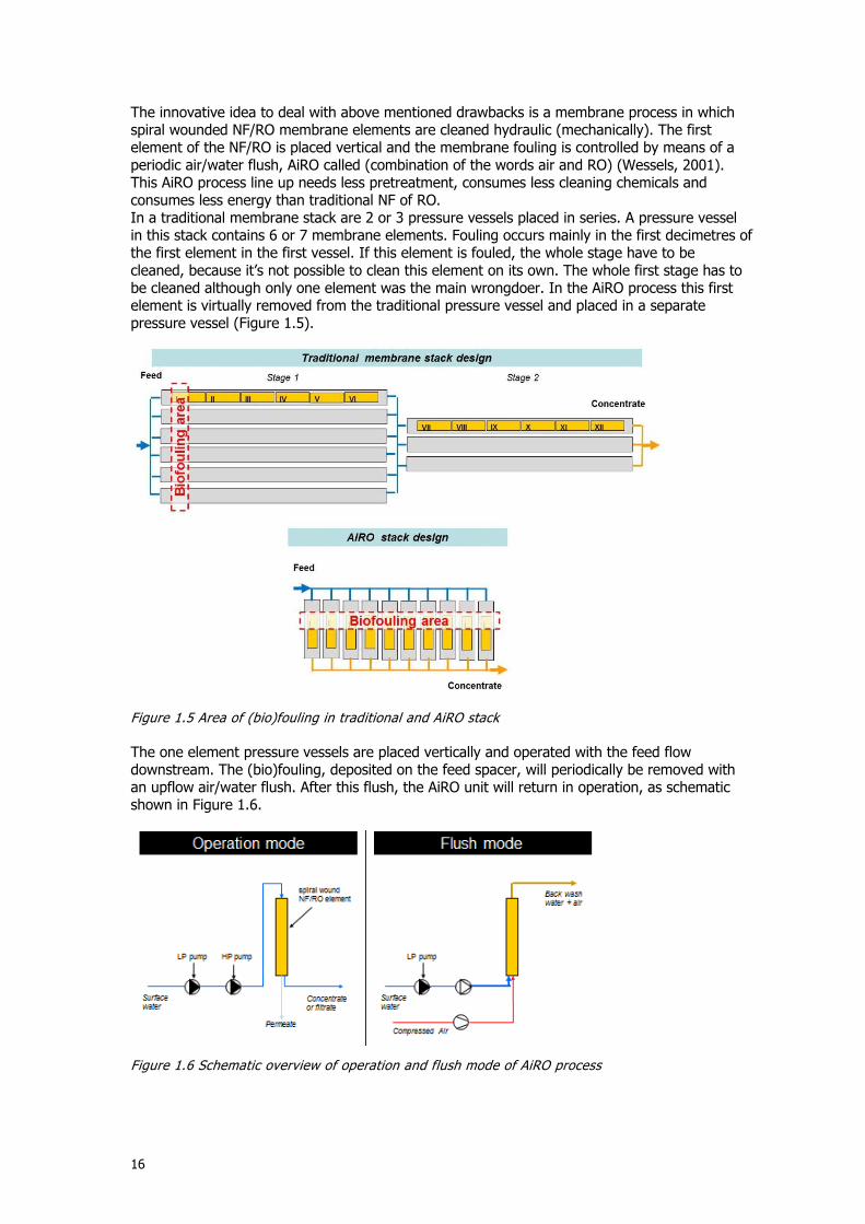
The innovative idea to deal with above mentioned drawbacks is a membrane process in which spiral wounded NF/RO membrane elements are cleaned hydraulic (mechanically). The first element of the NF/RO is placed vertical and the membrane fouling is controlled by means of a periodic air/water flush, AiRO called (combination of the words air and RO) (Wessels, 2001). This AiRO process line up needs less pretreatment, consumes less cleaning chemicals and consumes less energy than traditional NF of RO. In a traditional membrane stack are 2 or 3 pressure vessels placed in series. A pressure vessel in this stack contains 6 or 7 membrane elements. Fouling occurs mainly in the first decimetres of the first element in the first vessel. If this element is fouled, the whole stage have to be cleaned, because it’s not possible to clean this element on its own. The whole first stage has to be cleaned although only one element was the main wrongdoer. In the AiRO process this first element is virtually removed from the traditional pressure vessel and placed in a separate pressure vessel (Figure 1.5).

Figure 1.5 Area of (bio)fouling in traditional and AiRO stack

The one element pressure vessels are placed vertically and operated with the feed flow downstream. The (bio)fouling, deposited on the feed spacer, will periodically be removed with an upflow air/water flush. After this flush, the AiRO unit will return in operation, as schematic shown in Figure 1.6.

Figure 1.6 Schematic overview of operation and flush mode of AiRO process

17

Parameters that influence the AiRO process are: Pretreatment intensity; Procedure of flush, which steps does it contain; Duration of the flush steps; Flush interval; Water and air velocity and ratio during flush; Feed water quality; Additional chemical cleaning. Relevant research that has taken place on this topic will be discussed in the next paragraph.

1.7 Literature review

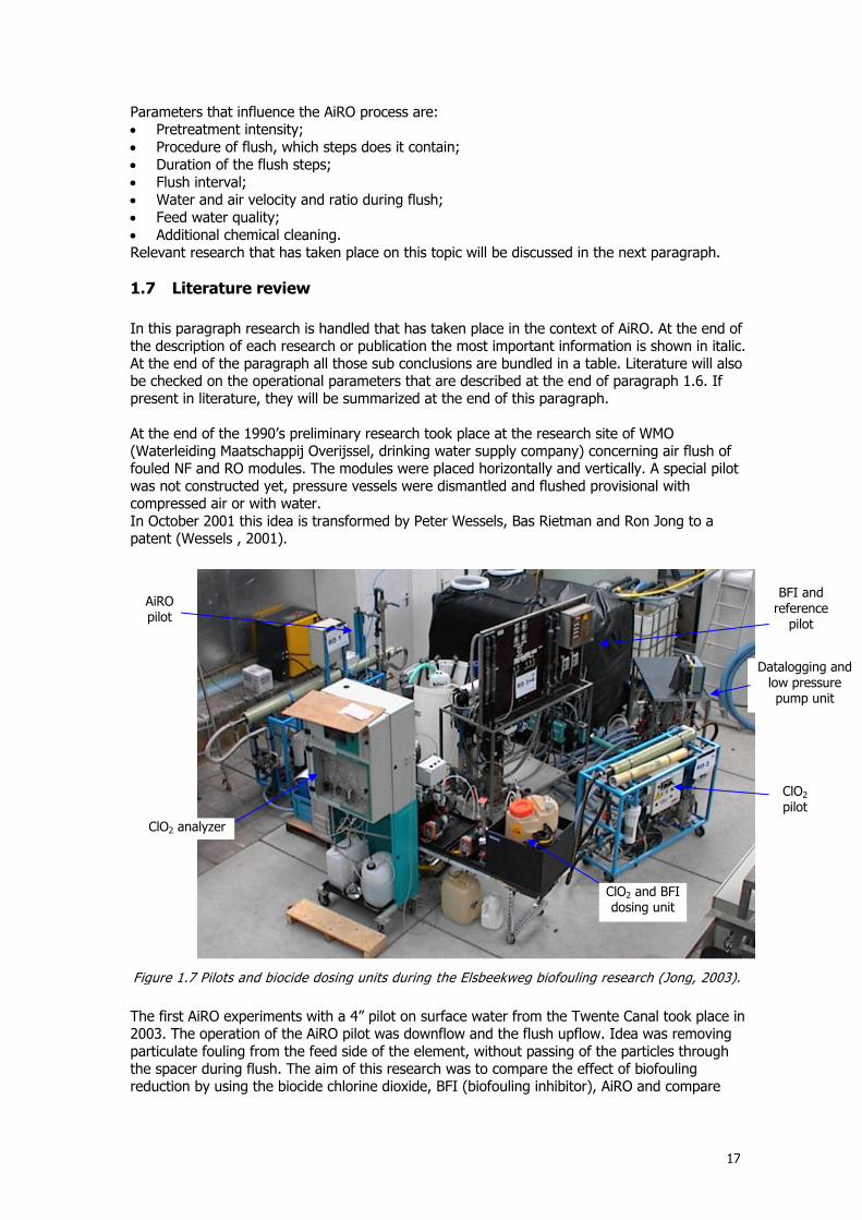
In this paragraph research is handled that has taken place in the context of AiRO. At the end of the description of each research or publication the most important information is shown in italic. At the end of the paragraph all those sub conclusions are bundled in a table. Literature will also be checked on the operational parameters that are described at the end of paragraph 1.6. If present in literature, they will be summarized at the end of this paragraph. At the end of the 1990’s preliminary research took place at the research site of WMO (Waterleiding Maatschappij Overijssel, drinking water supply company) concerning air flush of fouled NF and RO modules. The modules were placed horizontally and vertically. A special pilot was not constructed yet, pressure vessels were dismantled and flushed provisional with compressed air or with water. In October 2001 this idea is transformed by Peter Wessels, Bas Rietman and Ron Jong to a patent (Wessels , 2001).

The first AiRO experiments with a 4” pilot on surface water from the Twente Canal took place in 2003. The operation of the AiRO pilot was downflow and the flush upflow. Idea was removing particulate fouling from the feed side of the element, without passing of the particles through the spacer during flush. The aim of this research was to compare the effect of biofouling reduction by using the biocide chlorine dioxide, BFI (biofouling inhibitor), AiRO and compare

AiRO pilot

ClO2 analyzer

ClO2 and BFI dosing unit

ClO2 pilot

BFI and reference

pilot pilot

Datalogging and low pressure pump unit

Figure 1.7 Pilots and biocide dosing units during the Elsbeekweg biofouling research (Jong, 2003).

18

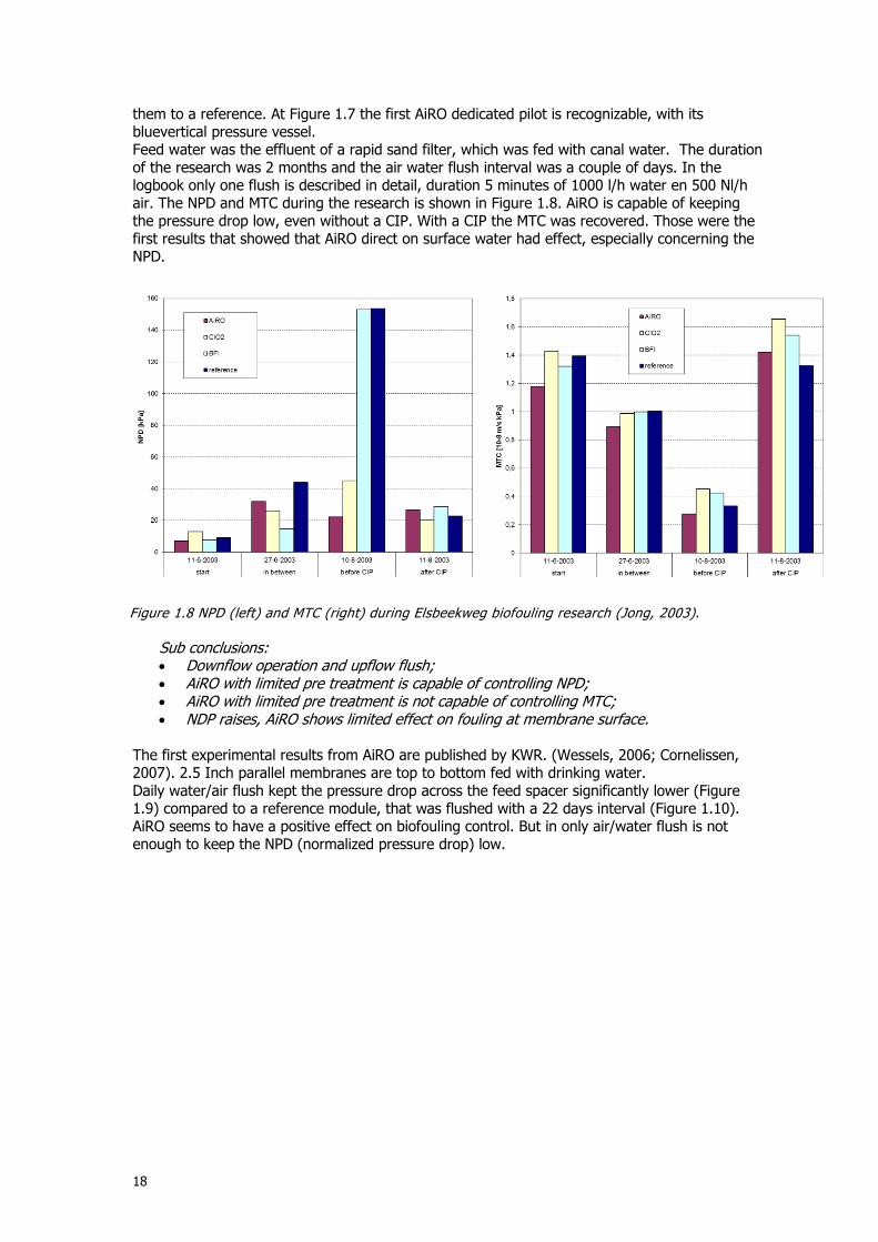
them to a reference. At Figure 1.7 the first AiRO dedicated pilot is recognizable, with its bluevertical pressure vessel. Feed water was the effluent of a rapid sand filter, which was fed with canal water. The duration of the research was 2 months and the air water flush interval was a couple of days. In the logbook only one flush is described in detail, duration 5 minutes of 1000 l/h water en 500 Nl/h air. The NPD and MTC during the research is shown in Figure 1.8. AiRO is capable of keeping the pressure drop low, even without a CIP. With a CIP the MTC was recovered. Those were the first results that showed that AiRO direct on surface water had effect, especially concerning the NPD.

Sub conclusions: Downflow operation and upflow flush; AiRO with limited pre treatment is capable of controlling NPD; AiRO with limited pre treatment is not capable of controlling MTC; NDP raises, AiRO shows limited effect on fouling at membrane surface.

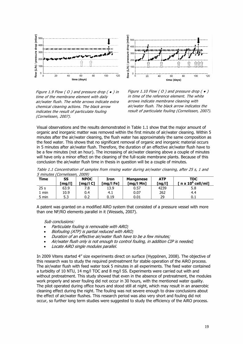
The first experimental results from AiRO are published by KWR. (Wessels, 2006; Cornelissen, 2007). 2.5 Inch parallel membranes are top to bottom fed with drinking water. Daily water/air flush kept the pressure drop across the feed spacer significantly lower (Figure 1.9) compared to a reference module, that was flushed with a 22 days interval (Figure 1.10). AiRO seems to have a positive effect on biofouling control. But in only air/water flush is not enough to keep the NPD (normalized pressure drop) low.

Figure 1.8 NPD (left) and MTC (right) during Elsbeekweg biofouling research (Jong, 2003).

19

Visual observations and the results demonstrated in Table 1.1 show that the major amount of organic and inorganic matter was removed within the first minute of air/water cleaning. Within 5 minutes after the air/water cleaning, the flush water has approximately the same composition as the feed water. This shows that no significant removal of organic and inorganic material occurs in 5 minutes after air/water flush. Therefore, the duration of an effective air/water flush have to be a few minutes (not an hour). The increasing of air/water cleaning above a couple of minutes will have only a minor effect on the cleaning of the full-scale membrane plants. Because of this conclusion the air/water flush time in thesis in question will be a couple of minutes.

Table 1.1 Concentration of samples from rinsing water during air/water cleaning, after 25 s, 1 and

5 minutes (Cornelissen, 2009) Time SS

[mg/l] NPOC

[mg/l C] Iron

[mg/l Fe] Manganese [mg/l Mn]

ATP [ng/l]

TDC [ n x 106 cell/ml]

25 s 1 min 5 min

63.9 10.9 5.3

7.8 0.4 0.2

13.9 4.1 0.19

0.57 0.07 0.01

4239 262 29

5.8 4.4 0.1

A patent was granted on a modified AiRO system that consisted of a pressure vessel with more than one NF/RO elements parallel in it (Wessels, 2007).

Sub conclusions: Particulate fouling is removable with AiRO; Biofouling (ATP) is partial reduced with AiRO; Duration of an effective air/water flush have to be a few minutes; Air/water flush only is not enough to control fouling, in addition CIP is needed; Locate AiRO single modules parallel.

In 2009 Vitens started 4” size experiments direct on surface (Hyppönen, 2008). The objective of this research was to study the required pretreatment for stable operation of the AiRO process. The air/water flush with feed water took 5 minutes in all experiments. The feed water contained a turbidity of 10 NTU, 14 mg/l TOC and 8 mg/l SS. Experiments were carried out with and without pretreatment. This study showed that even in the absence of pretreatment, the modules work properly and sever fouling did not occur in 30 hours, with the mentioned water quality. The pilot operated during office hours and stood still at night, which may result in an anaerobic cleaning effect during the night. The fouling was not severe enough to draw conclusions about the effect of air/water flushes. This research period was also very short and fouling did not occur, so further long term studies were suggested to study the efficiency of the AiRO process.

Figure 1.10 Flow ( O ) and pressure drop ( ● )

in time of the reference element. The white

arrows indicate membrane cleaning with

air/water flush. The black arrow indicates the

result of particulate fouling (Cornelissen, 2007).

Figure 1.9 Flow ( O ) and pressure drop ( ● ) in

time of the membrane element with daily

air/water flush. The white arrows indicate extra

chemical cleaning actions. The black arrow

indicates the result of particulate fouling

(Cornelissen, 2007).

20

Sub conclusions: It is possible to treat surface water with reverse osmosis membranes, even in absence

of pretreatment; Long term studies are suggested

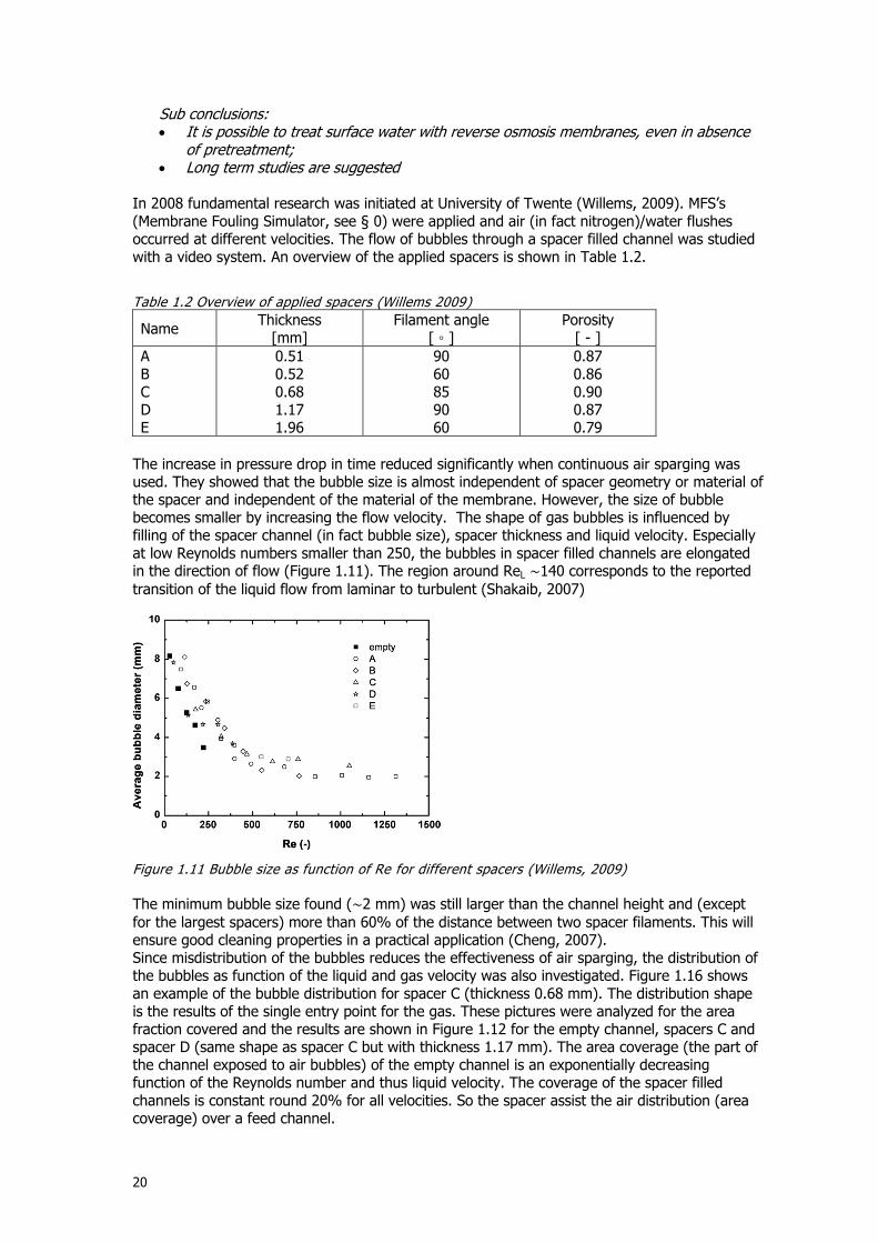
In 2008 fundamental research was initiated at University of Twente (Willems, 2009). MFS’s (Membrane Fouling Simulator, see § 0) were applied and air (in fact nitrogen)/water flushes occurred at different velocities. The flow of bubbles through a spacer filled channel was studied with a video system. An overview of the applied spacers is shown in Table 1.2.

Table 1.2 Overview of applied spacers (Willems 2009)

Name Thickness

[mm] Filament angle

[ ◦ ] Porosity

[ - ]

A B C D E

0.51 0.52 0.68 1.17 1.96

90 60 85 90 60

0.87 0.86 0.90 0.87 0.79

The increase in pressure drop in time reduced significantly when continuous air sparging was used. They showed that the bubble size is almost independent of spacer geometry or material of the spacer and independent of the material of the membrane. However, the size of bubble becomes smaller by increasing the flow velocity. The shape of gas bubbles is influenced by filling of the spacer channel (in fact bubble size), spacer thickness and liquid velocity. Especially at low Reynolds numbers smaller than 250, the bubbles in spacer filled channels are elongated in the direction of flow (Figure 1.11). The region around ReL ∼140 corresponds to the reported

transition of the liquid flow from laminar to turbulent (Shakaib, 2007)

Figure 1.11 Bubble size as function of Re for different spacers (Willems, 2009)

The minimum bubble size found (∼2 mm) was still larger than the channel height and (except

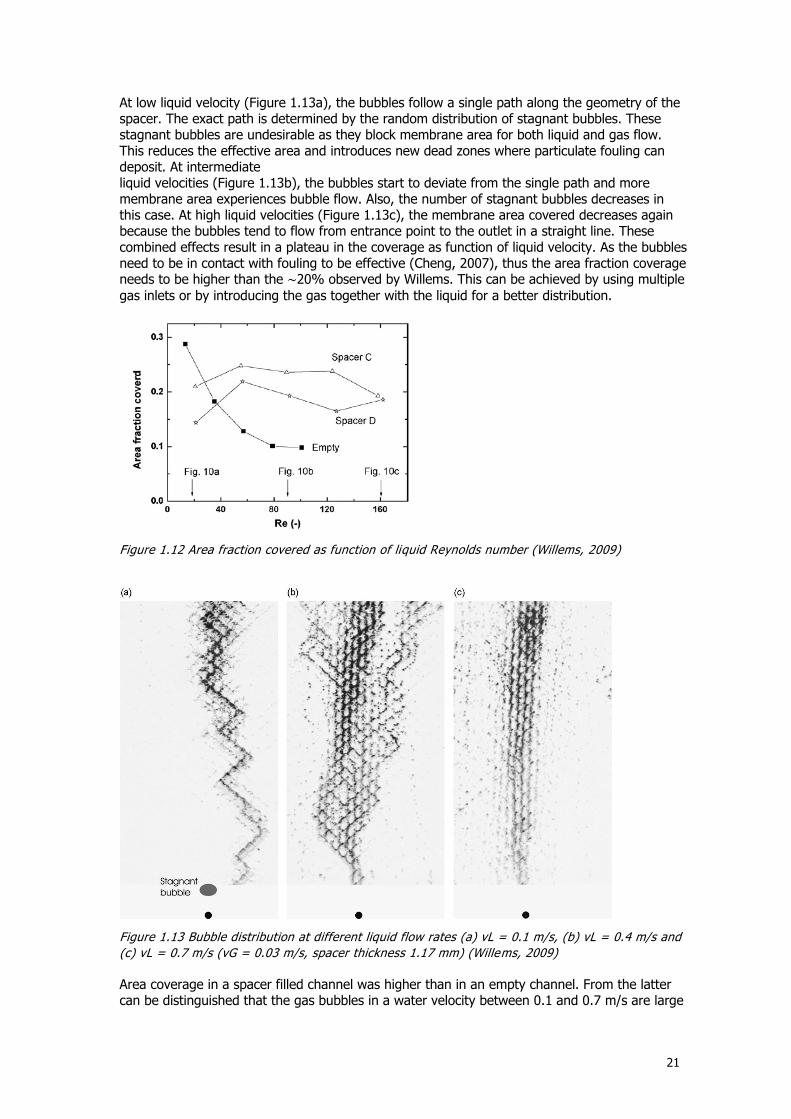
for the largest spacers) more than 60% of the distance between two spacer filaments. This will ensure good cleaning properties in a practical application (Cheng, 2007). Since misdistribution of the bubbles reduces the effectiveness of air sparging, the distribution of the bubbles as function of the liquid and gas velocity was also investigated. Figure 1.16 shows an example of the bubble distribution for spacer C (thickness 0.68 mm). The distribution shape is the results of the single entry point for the gas. These pictures were analyzed for the area fraction covered and the results are shown in Figure 1.12 for the empty channel, spacers C and spacer D (same shape as spacer C but with thickness 1.17 mm). The area coverage (the part of the channel exposed to air bubbles) of the empty channel is an exponentially decreasing function of the Reynolds number and thus liquid velocity. The coverage of the spacer filled channels is constant round 20% for all velocities. So the spacer assist the air distribution (area coverage) over a feed channel.

21

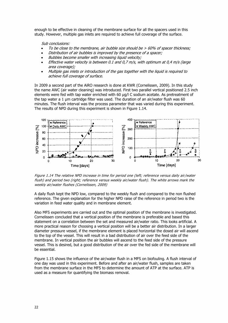
At low liquid velocity (Figure 1.13a), the bubbles follow a single path along the geometry of the spacer. The exact path is determined by the random distribution of stagnant bubbles. These stagnant bubbles are undesirable as they block membrane area for both liquid and gas flow. This reduces the effective area and introduces new dead zones where particulate fouling can deposit. At intermediate liquid velocities (Figure 1.13b), the bubbles start to deviate from the single path and more membrane area experiences bubble flow. Also, the number of stagnant bubbles decreases in this case. At high liquid velocities (Figure 1.13c), the membrane area covered decreases again because the bubbles tend to flow from entrance point to the outlet in a straight line. These combined effects result in a plateau in the coverage as function of liquid velocity. As the bubbles need to be in contact with fouling to be effective (Cheng, 2007), thus the area fraction coverage needs to be higher than the ∼20% observed by Willems. This can be achieved by using multiple

gas inlets or by introducing the gas together with the liquid for a better distribution.

Figure 1.12 Area fraction covered as function of liquid Reynolds number (Willems, 2009)

Figure 1.13 Bubble distribution at different liquid flow rates (a) vL = 0.1 m/s, (b) vL = 0.4 m/s and

(c) vL = 0.7 m/s (vG = 0.03 m/s, spacer thickness 1.17 mm) (Willems, 2009)

Area coverage in a spacer filled channel was higher than in an empty channel. From the latter can be distinguished that the gas bubbles in a water velocity between 0.1 and 0.7 m/s are large

22

enough to be effective in cleaning of the membrane surface for all the spacers used in this study. However, multiple gas inlets are required to achieve full coverage of the surface.

Sub conclusions: To be close to the membrane, air bubble size should be > 60% of spacer thickness; Distribution of air bubbles is improved by the presence of a spacer; Bubbles become smaller with increasing liquid velocity; Effective water velocity is between 0.1 and 0,7 m/s, with optimum at 0,4 m/s (large

area coverage); Multiple gas inlets or introduction of the gas together with the liquid is required to

achieve full coverage of surface. In 2009 a second part of the AiRO research is done at KWR (Cornelissen, 2009). In this study the name AWC (air water cleaning) was introduced. First two parallel vertical positioned 2.5 inch elements were fed with tap water enriched with 60 µg/l C sodium acetate. As pretreatment of the tap water a 1 µm cartridge filter was used. The duration of an air/water flush was 60 minutes. The flush interval was the process parameter that was varied during this experiment. The results of NPD during this experiment is shown in Figure 1.14.

Figure 1.14 The relative NPD increase in time for period one (left; reference versus daily air /water

flush) and period two (right; reference versus weekly air/water flush). The white arrows mark the

weekly air/water flushes (Cornelissen, 2009)

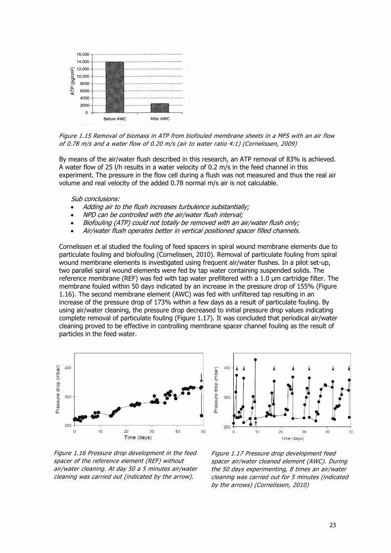
A daily flush kept the NPD low, compared to the weekly flush and compared to the non flushed reference. The given explanation for the higher NPD raise of the reference in period two is the variation in feed water quality and in membrane element. Also MFS experiments are carried out and the optimal position of the membrane is investigated. Cornelissen concluded that a vertical position of the membrane is preferable and based this statement on a correlation between the set and measured air/water ratio. This looks artificial. A more practical reason for choosing a vertical position will be a better air distribution. In a larger diameter pressure vessel, if the membrane element is placed horizontal the dosed air will ascend to the top of the vessel. This will result in a bad distribution of air over the feed side of the membrane. In vertical position the air bubbles will ascend to the feed side of the pressure vessel. This is desired, but a good distribution of the air over the fed side of the membrane will be essential. Figure 1.15 shows the influence of the air/water flush in a MFS on biofouling. A flush interval of one day was used in this experiment. Before and after an air/water flush, samples are taken from the membrane surface in the MFS to determine the amount of ATP at the surface. ATP is used as a measure for quantifying the biomass removal.

23

Figure 1.15 Removal of biomass in ATP from biofouled membrane sheets in a MFS with an air flow

of 0.78 m/s and a water flow of 0.20 m/s (air to water ratio 4:1) (Cornelissen, 2009)

By means of the air/water flush described in this research, an ATP removal of 83% is achieved. A water flow of 25 l/h results in a water velocity of 0.2 m/s in the feed channel in this experiment. The pressure in the flow cell during a flush was not measured and thus the real air volume and real velocity of the added 0.78 normal m/s air is not calculable.

Sub conclusions: Adding air to the flush increases turbulence substantially; NPD can be controlled with the air/water flush interval; Biofouling (ATP) could not totally be removed with an air/water flush only; Air/water flush operates better in vertical positioned spacer filled channels.

Cornelissen et al studied the fouling of feed spacers in spiral wound membrane elements due to particulate fouling and biofouling (Cornelissen, 2010). Removal of particulate fouling from spiral wound membrane elements is investigated using frequent air/water flushes. In a pilot set-up, two parallel spiral wound elements were fed by tap water containing suspended solids. The reference membrane (REF) was fed with tap water prefiltered with a 1.0 μm cartridge filter. The membrane fouled within 50 days indicated by an increase in the pressure drop of 155% (Figure 1.16). The second membrane element (AWC) was fed with unfiltered tap resulting in an increase of the pressure drop of 173% within a few days as a result of particulate fouling. By using air/water cleaning, the pressure drop decreased to initial pressure drop values indicating complete removal of particulate fouling (Figure 1.17). It was concluded that periodical air/water cleaning proved to be effective in controlling membrane spacer channel fouling as the result of particles in the feed water.

Figure 1.16 Pressure drop development in the feed

spacer of the reference element (REF) without

air/water cleaning. At day 50 a 5 minutes air/water

cleaning was carried out (indicated by the arrow).

Figure 1.17 Pressure drop development feed

spacer air/water cleaned element (AWC). During

the 50 days experimenting, 8 times an air/water

cleaning was carried out for 5 minutes (indicated

by the arrows) (Cornelissen, 2010)

24

Sub conclusion: Periodical air/water cleaning proved to be effective in controlling membrane spacer

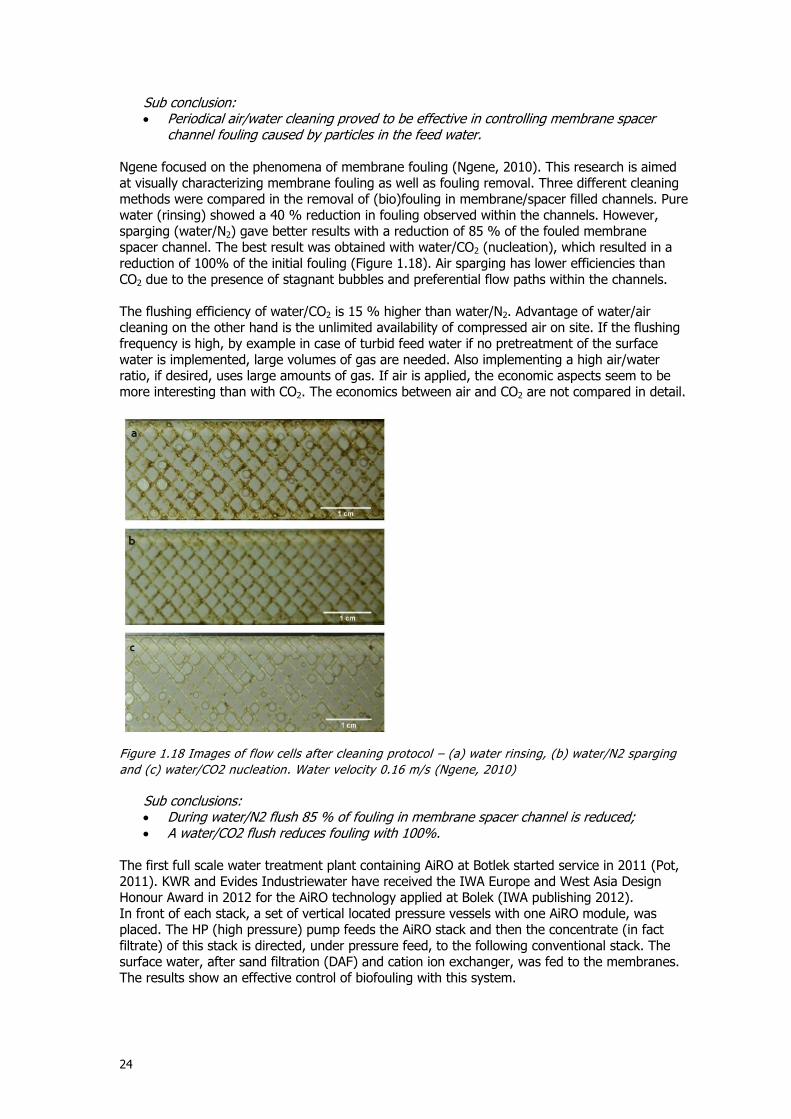
channel fouling caused by particles in the feed water. Ngene focused on the phenomena of membrane fouling (Ngene, 2010). This research is aimed at visually characterizing membrane fouling as well as fouling removal. Three different cleaning methods were compared in the removal of (bio)fouling in membrane/spacer filled channels. Pure water (rinsing) showed a 40 % reduction in fouling observed within the channels. However, sparging (water/N2) gave better results with a reduction of 85 % of the fouled membrane spacer channel. The best result was obtained with water/CO2 (nucleation), which resulted in a reduction of 100% of the initial fouling (Figure 1.18). Air sparging has lower efficiencies than CO2 due to the presence of stagnant bubbles and preferential flow paths within the channels. The flushing efficiency of water/CO2 is 15 % higher than water/N2. Advantage of water/air cleaning on the other hand is the unlimited availability of compressed air on site. If the flushing frequency is high, by example in case of turbid feed water if no pretreatment of the surface water is implemented, large volumes of gas are needed. Also implementing a high air/water ratio, if desired, uses large amounts of gas. If air is applied, the economic aspects seem to be more interesting than with CO2. The economics between air and CO2 are not compared in detail.

Figure 1.18 Images of flow cells after cleaning protocol – (a) water rinsing, (b) water/N2 sparging

and (c) water/CO2 nucleation. Water velocity 0.16 m/s (Ngene, 2010)

Sub conclusions: During water/N2 flush 85 % of fouling in membrane spacer channel is reduced; A water/CO2 flush reduces fouling with 100%.

The first full scale water treatment plant containing AiRO at Botlek started service in 2011 (Pot, 2011). KWR and Evides Industriewater have received the IWA Europe and West Asia Design Honour Award in 2012 for the AiRO technology applied at Bolek (IWA publishing 2012). In front of each stack, a set of vertical located pressure vessels with one AiRO module, was placed. The HP (high pressure) pump feeds the AiRO stack and then the concentrate (in fact filtrate) of this stack is directed, under pressure feed, to the following conventional stack. The surface water, after sand filtration (DAF) and cation ion exchanger, was fed to the membranes. The results show an effective control of biofouling with this system.

25

Sub conclusions: The AiRO process functions in Botlek as prefiltration of a conventional RO stack; The HP pump feeds both AiRO and following stack.

Wibisono started studying the AiRO process involving the optimal use of air/water cleaning of spiral wound membrane elements in 2010. The following parameters were studied (1) air/water ratio, (2) air and water velocity, (3) air/water cleaning duration and (4) air/water cleaning frequency. Research questions will be investigated using CFD modelling parallel to laboratory tests, using membrane fouling simulators and small-scale 2.5-inch spiral wound membrane elements. His impressive paper describes and analyzes 195 scientific papers about two-phase flow in any type of membrane filtration (Wibisono, 2014). Collected data was normalized based on gas and liquid superficial velocities, gas/liquid ratio and feed types, trans-membrane pressure and membrane module type in order to make a fair comparison and identify general characteristics. The objective was to identify key factors in the application of two-phase flows in aqueous separation and purification processes, deliver new insights in how to optimize operations for implementation of this technology in the industry, and provide a brief overview of current commercial applications. Mainly MF/UF applications are described, the NF/RO part of this paper contains 5 references, in fact, is the research of Cornelissen, Willems and Ngene, described here before.

Sub conclusions: Two-phase flow cleaning is able to remove voluminous and filamentous biofilm

structures attached to membrane and feed spacer surfaces, lowers the pressure drop and decreases biomass concentration more than by application of chemical cleaning.

Haidari started in 2011 on the subject One Step Membrane filtration (OSMF) (Haidari, 2011). The membrane filtration in this project in fact is an AiRO direct on surface water. More efficient operation of membrane filtration and as result lower operational costs are the main goal of this study. This will be achieved with the real time visualization of membrane filtration mechanism, interaction of membrane with particles, accumulation of these particles on the membrane and fouling of membrane. Visual instruments such as Particle Image Velocimetry (PIV) are applied for a better understanding of the membrane filtration, membrane fouling and cleaning. This study paves the way for total elimination of pretreatment steps in drinking water. The sub conclusions in above described literature are summarized in Table 1.3.

26

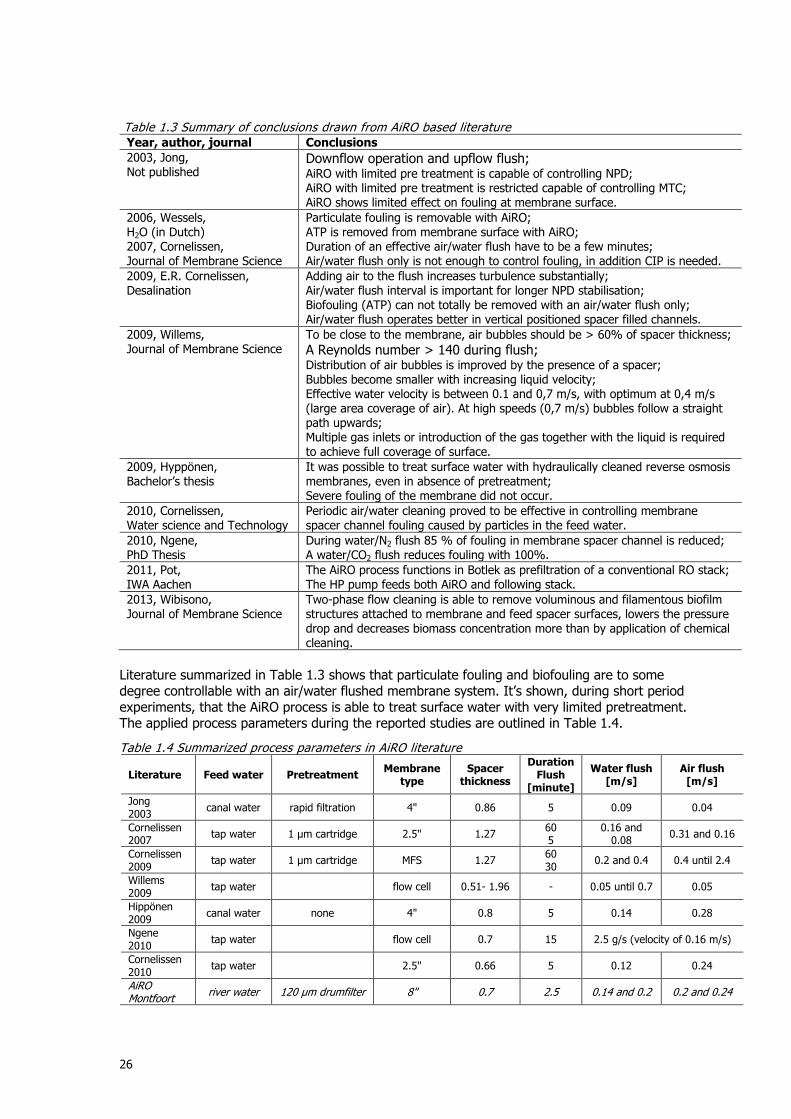
Table 1.3 Summary of conclusions drawn from AiRO based literature Year, author, journal Conclusions

2003, Jong, Not published

Downflow operation and upflow flush; AiRO with limited pre treatment is capable of controlling NPD; AiRO with limited pre treatment is restricted capable of controlling MTC; AiRO shows limited effect on fouling at membrane surface.

2006, Wessels, H2O (in Dutch) 2007, Cornelissen, Journal of Membrane Science

Particulate fouling is removable with AiRO; ATP is removed from membrane surface with AiRO; Duration of an effective air/water flush have to be a few minutes; Air/water flush only is not enough to control fouling, in addition CIP is needed.

2009, E.R. Cornelissen, Desalination

Adding air to the flush increases turbulence substantially; Air/water flush interval is important for longer NPD stabilisation; Biofouling (ATP) can not totally be removed with an air/water flush only; Air/water flush operates better in vertical positioned spacer filled channels.

2009, Willems, Journal of Membrane Science

To be close to the membrane, air bubbles should be > 60% of spacer thickness;

A Reynolds number > 140 during flush; Distribution of air bubbles is improved by the presence of a spacer; Bubbles become smaller with increasing liquid velocity; Effective water velocity is between 0.1 and 0,7 m/s, with optimum at 0,4 m/s (large area coverage of air). At high speeds (0,7 m/s) bubbles follow a straight path upwards; Multiple gas inlets or introduction of the gas together with the liquid is required to achieve full coverage of surface.

2009, Hyppönen, Bachelor’s thesis

It was possible to treat surface water with hydraulically cleaned reverse osmosis membranes, even in absence of pretreatment; Severe fouling of the membrane did not occur.

2010, Cornelissen, Water science and Technology

Periodic air/water cleaning proved to be effective in controlling membrane spacer channel fouling caused by particles in the feed water.

2010, Ngene, PhD Thesis

During water/N2 flush 85 % of fouling in membrane spacer channel is reduced; A water/CO2 flush reduces fouling with 100%.

2011, Pot, IWA Aachen

The AiRO process functions in Botlek as prefiltration of a conventional RO stack; The HP pump feeds both AiRO and following stack.

2013, Wibisono, Journal of Membrane Science

Two-phase flow cleaning is able to remove voluminous and filamentous biofilm structures attached to membrane and feed spacer surfaces, lowers the pressure drop and decreases biomass concentration more than by application of chemical cleaning.

Literature summarized in Table 1.3 shows that particulate fouling and biofouling are to some degree controllable with an air/water flushed membrane system. It’s shown, during short period experiments, that the AiRO process is able to treat surface water with very limited pretreatment. The applied process parameters during the reported studies are outlined in Table 1.4.

Table 1.4 Summarized process parameters in AiRO literature

Literature Feed water Pretreatment Membrane

type Spacer

thickness

Duration Flush

[minute]

Water flush [m/s]

Air flush [m/s]

Jong 2003

canal water rapid filtration 4" 0.86 5 0.09 0.04

Cornelissen 2007

tap water 1 µm cartridge 2.5" 1.27 60 5

0.16 and 0.08

0.31 and 0.16

Cornelissen 2009

tap water 1 µm cartridge MFS 1.27 60 30

0.2 and 0.4 0.4 until 2.4

Willems 2009

tap water

flow cell 0.51- 1.96 - 0.05 until 0.7 0.05

Hippönen 2009

canal water none 4" 0.8 5 0.14 0.28

Ngene 2010

tap water

flow cell 0.7 15 2.5 g/s (velocity of 0.16 m/s)

Cornelissen 2010

tap water

2.5" 0.66 5 0.12 0.24

AiRO Montfoort

river water 120 µm drumfilter 8" 0.7 2.5 0.14 and 0.2 0.2 and 0.24

27

The content of Table 1.3 and Table 1.4 will be used to define the objectives for the AiRO research in this thesis.

1.8 Objectives

With the help of the literature that is outlined in the previous paragraph, info is collected about the AiRO process. But there still are questions that have to be answered before a reliable process design based on AiRO can be made. Boundary conditions of the process are: A vertical arrangement of the membrane, downflow operation and upflow flush; A Reynolds number > 140 during flush to achieve a turbulent flow in the feed spacer; A water velocity during flush between 0.1 and 0.7 m/s, with optimum at 0.4 m/s, to achieve

sufficient area coverage of bubbles; multiple gas inlets or introduction of the gas together with the liquid to achieve full coverage

of the membrane and feed spacer surface. an additional CIP to remove fouling. Objectives for AiRO research will be based on the process parameters outlined in § 1.6: Pretreatment intensity Surface water has been applied as source water without pre treatment (Hippönen, 2009). Hypothesis is that the pretreatment only has to remove particles that can not pass the membrane feed spacer. Question: Is a treatment step that only removes particles sufficient as pretreatment for an AiRO process on surface water? Procedure of flush, of which steps does it contain From the flush steps, in literature only the air/water flush (combined flush) is described. During a flush trapped particles and biological debris have to be removed. There seems to be consistence between a rapid sand filter and a vertical placed AiRO membrane element. A rapid sand filter backwash procedure consists of 3 steps; a preflush step with water only, a combined flush step with water and air and a postflush step with water only. Idea is to apply the same type of procedure on the AiRO process. Question: Which flush procedure will result in a stable operation of the AiRO process? Duration of the flush steps If the procedure of the flush is known, what will be the duration of the individual steps of it? The duration of the combined flush is between 5 and 60 minutes as described in literature (Table 1.4). The duration of pre- and postflush is not mentioned in literature and have to be studied from scratch. The duration of the combined step is in literature such varied that it has to be determined in detail. Question: what will be the duration of defined flush steps? Flush interval The applied flush interval in studies has been a day, 30 hours and a week (Jong, 2003; Cornelissen, 2009; Hippönen, 2009). Question: What is a time interval between flushes that provides a stable operation of the AiRO process? Water and air velocity and ratio during flush During flush steps air and/or water is pressed through the feed spacer to remove debris from it and from the membrane surface. The velocity of air and water during the combined flush varied between resp. 0.04 and 2.4 m/s and 0.09 and 0.8 m/s (Table 1.4). With 0,4 m/s of water the area coverage of the air bubbles is sufficient (Willems, 2009) and a Reynolds number > 140 gives turbid flow in a membrane spacer (Shakaib, 2007). Those figures will be the base for the determination of the flush intensity. Question: What will be the water and air velocity (and ratio) during flush?

28

Feed water quality Different feed water qualities are applied in described studies. The most extreme feed water is surface water with limited pretreatment (Jong, 2003; Hippönen, 2009). Question: What is the influence of feed water quality on the AiRO process? Additional chemical cleaning In some studies that take place during a research period longer than a month also a CIP has been a part of the operation of the AiRO process (Jong, 2003; Cornelissen, 2007). If limited treated surface water is applied as feed water of AiRO, certainly a regular CIP have to take place to maintain a stable operation. Question: Which CIP procedure is preferred and when will it take place? Economical aspects The design of a drinking water treatment on surface water based on AiRO differs dramatic from the design of a conventional surface water treatment based on membrane filtration. AiRO is a new way of thinking. The economic aspects of a conventional and an AiRO scenario will be calculated and compared. Question: What does a surface water treatment based on the AiRO concept look like and what are the rough economic aspects of it? Goal of the AIRO research described in this TU Delft thesis is to answer above described questions in a long term applicable research. This research will take place in two stages. Goal of the first period is to check and determine the operational aspects of the pilot plant. In the first period the settings of the pilots, by example the flush procedure, may be varied to determine a stable operation. In the second period the settings of the pilots will remain as fixed as possible. Goal of this period is to keep the operation stable and to learn more about the relation between feed water quality and operational aspects.

1.9 Outline

Chapter 1 gives a brief description of the water treatment technology “membrane filtration” and of the AiRO process. The usefulness of the AiRO research in this thesis is substantiated and the research questions are outlined. In chapter 2 the approach of the research is described, inclusive the applied methods. The results are processed in detail in chapter 3 and discussed in chapter 4. Finally chapter 5 contains the conclusions and recommendations of this AiRO research.

29

2 Materials and methods

2.1 Research location Montfoort

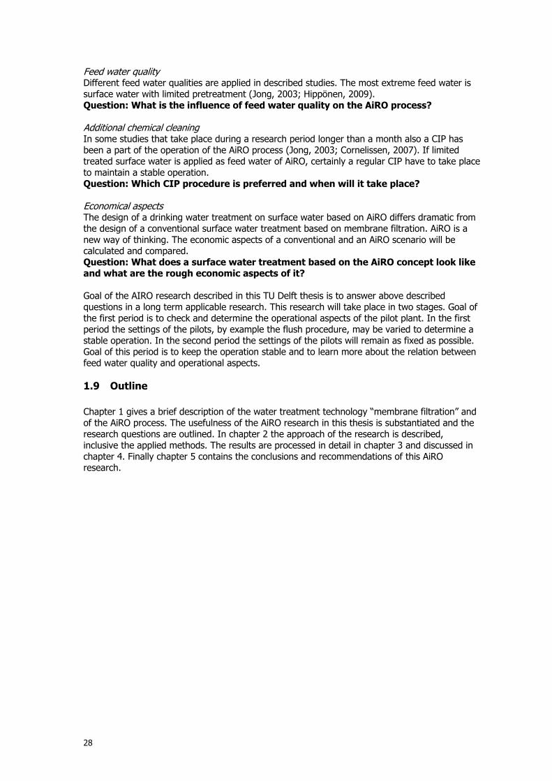
Location for the AiRO research is a formal groundwater treatment of Vitens at the banks of the Hollandse IJssel river in Montfoort near Utrecht (Figure 2.1).

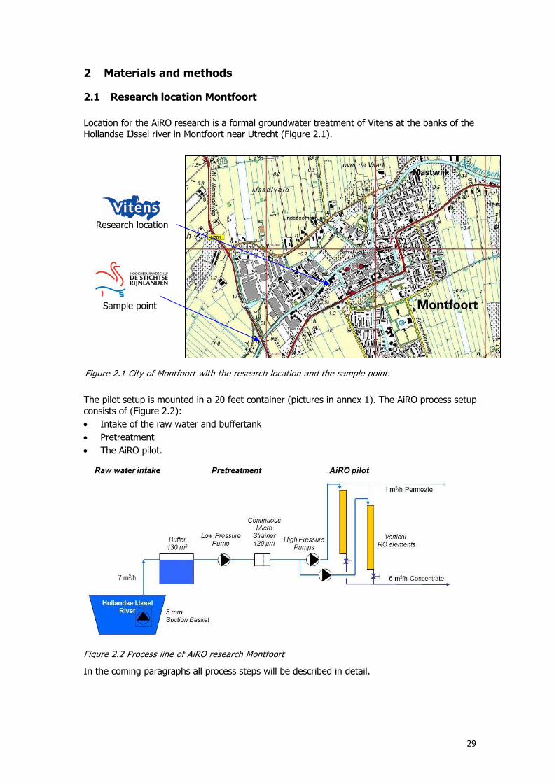
The pilot setup is mounted in a 20 feet container (pictures in annex 1). The AiRO process setup consists of (Figure 2.2):

Intake of the raw water and buffertank

Pretreatment

The AiRO pilot.

In the coming paragraphs all process steps will be described in detail.

City 1 Figure 2.1 City of Montfoort with the research location and the sample point.

Research location

Sample point

Figure 2.2 Process line of AiRO research Montfoort

30

2.2 Raw water intake

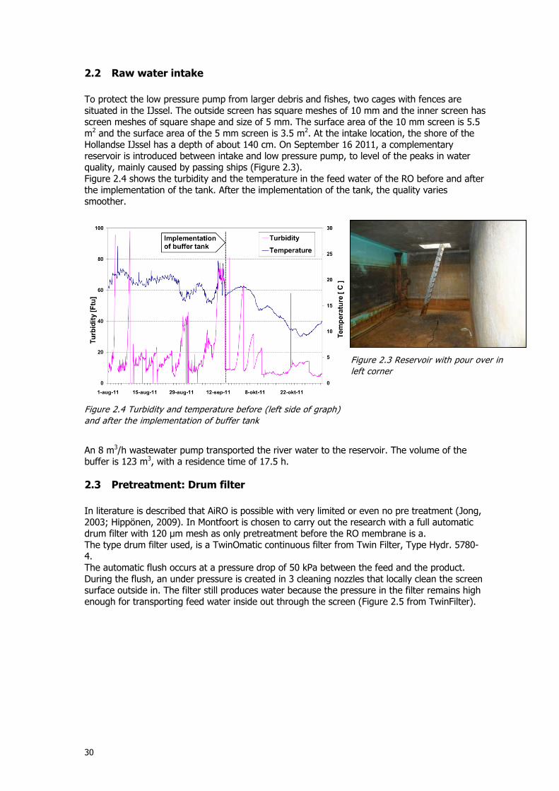
To protect the low pressure pump from larger debris and fishes, two cages with fences are situated in the IJssel. The outside screen has square meshes of 10 mm and the inner screen has screen meshes of square shape and size of 5 mm. The surface area of the 10 mm screen is 5.5 m2 and the surface area of the 5 mm screen is 3.5 m2. At the intake location, the shore of the Hollandse IJssel has a depth of about 140 cm. On September 16 2011, a complementary reservoir is introduced between intake and low pressure pump, to level of the peaks in water quality, mainly caused by passing ships (Figure 2.3). Figure 2.4 shows the turbidity and the temperature in the feed water of the RO before and after the implementation of the tank. After the implementation of the tank, the quality varies smoother.

An 8 m3/h wastewater pump transported the river water to the reservoir. The volume of the buffer is 123 m3, with a residence time of 17.5 h.

2.3 Pretreatment: Drum filter

In literature is described that AiRO is possible with very limited or even no pre treatment (Jong, 2003; Hippönen, 2009). In Montfoort is chosen to carry out the research with a full automatic drum filter with 120 µm mesh as only pretreatment before the RO membrane is a. The type drum filter used, is a TwinOmatic continuous filter from Twin Filter, Type Hydr. 5780-4. The automatic flush occurs at a pressure drop of 50 kPa between the feed and the product. During the flush, an under pressure is created in 3 cleaning nozzles that locally clean the screen surface outside in. The filter still produces water because the pressure in the filter remains high enough for transporting feed water inside out through the screen (Figure 2.5 from TwinFilter).

Figure 2.4 Turbidity and temperature before (left side of graph)

and after the implementation of buffer tank

Figure 2.3 Reservoir with pour over in

left corner

31

Figure 2.5 Schematic overview of an continuous drum filter (l) and detail of nozzle (r) (TwinFilter)

2.4 AiRO unit

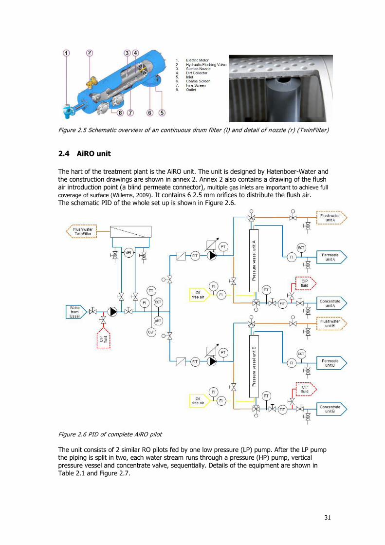
The hart of the treatment plant is the AiRO unit. The unit is designed by Hatenboer-Water and the construction drawings are shown in annex 2. Annex 2 also contains a drawing of the flush air introduction point (a blind permeate connector), multiple gas inlets are important to achieve full

coverage of surface (Willems, 2009). It contains 6 2.5 mm orifices to distribute the flush air. The schematic PID of the whole set up is shown in Figure 2.6.

Figure 2.6 PID of complete AiRO pilot

The unit consists of 2 similar RO pilots fed by one low pressure (LP) pump. After the LP pump the piping is split in two, each water stream runs through a pressure (HP) pump, vertical pressure vessel and concentrate valve, sequentially. Details of the equipment are shown in Table 2.1 and Figure 2.7.

32

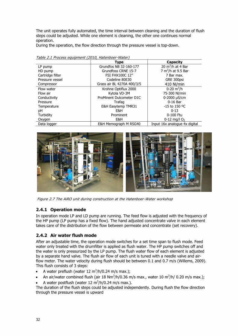
The unit operates fully automated, the time interval between cleaning and the duration of flush steps could be adjusted. While one element is cleaning, the other one continues normal operation. During the operation, the flow direction through the pressure vessel is top-down.

Table 2.1 Process equipment (2010, Hatenboer-Water) Type Capacity

LP pump HD pump Cartridge filter Pressure vessel Compressor

Grundfos NB 32-160-177 Grundfoss CRNE 15-7

FSI FHX100C 12” Codeline 80E30

Grass air BL 4270A 400/3/5

20 m3/h at 4 Bar 7 m3/h at 9.5 Bar

7 Bar max. GRE 300psi

410 Nl/min

Flow water Flow air Conductivity Pressure Temperature pH Turbidity Oxygen

Krohne Optiflux 2000 Kytola VD-3M

ProMinent Dulcometer D1C Trafag

E&H Easytemp TMR31 E&H

Prominent E&H

0-20 m3/h 75-300 Nl/min 0-2000 µS/cm

0-16 Bar -15 to 150 ºC

0-13 0-100 Ftu

0-12 mg/l O2

Data logger E&H Memograph M RSG40 Input 16x analogue 4x digital

2.4.1 Operation mode

In operation mode LP and LD pump are running. The feed flow is adjusted with the frequency of the HP pump (LP pump has a fixed flow). The hand adjusted concentrate valve in each element takes care of the distribution of the flow between permeate and concentrate (set recovery).

2.4.2 Air water flush mode

After an adjustable time, the operation mode switches for a set time span to flush mode. Feed water only treated with the drumfilter is applied as flush water. The HP pump switches off and the water is only pressurized by the LP pump. The flush water flow of each element is adjusted by a separate hand valve. The flush air flow of each unit is tuned with a needle valve and air-flow meter. The water velocity during flush should be between 0.1 and 0.7 m/s (Willems, 2009). This flush consists of 3 steps:

A water preflush (water 12 m3/h/0.24 m/s max.);

An air/water combined flush (air 18 Nm3/h/0.36 m/s max., water 10 m3/h/ 0.20 m/s max.);

A water postflush (water 12 m3/h/0.24 m/s max.). The duration of the flush steps could be adjusted independently. During flush the flow direction through the pressure vessel is upward

Figure 2.7 The AiRO unit during construction at the Hatenboer-Water workshop

33

The flush air is produced with an oil free Grass-Air compressor with a capacity of 410 l/min and 3 kW power. The compressed air is cleaned with 2 subsequent particle filters of 1 µm and 0.01 µm and an activated carbon filter (removal of oil). The air is finally stored at a pressure of 10 Bar in a 270 l tank with automatic condensate drain.

2.4.3 CIP (Clean In Place)

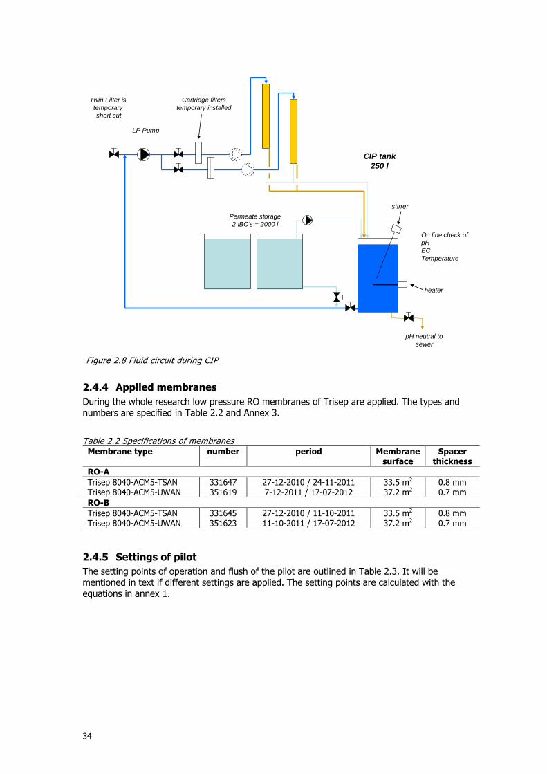
A CIP is essential (Jong, 2003; Cornelissen, 2007) and is a manually-operated action. The whole pilot is taken out of action and a 250 l CIP tank is mounted between the LP pump en the concentrate outlet of the unit to be cleaned. The LP pump serves as recirculation pump and temporary 10 µm cartridge filters are mounted in the normal empty housings (Figure 2.8). The max recirculation flow is 10 m3/h (20 m/s). Main part of the CIP solution is permeate of AiRO pilots and the pH is with chemicals adjusted between 2 and 12. The temperature of the CIP solution can be raised to 40 °C and the flow, pH, temperature and conductivity of the solution are gauged during a CIP. The waste of CIP solution is adjusted to a pH between 6.5 and 9.0 with NaOH or HCl and disposed to the sewer. A total overview of the applied chemicals gives: Acid cleaning:

Citric acid 50%, add until a 2% volume concentration, pH between 2.0 and 3.0;

NC136, add until a 1 % volume concentration, pH between 2.0 and 2.5. NovoClean 136 is an acid cleaning agent based on complexing agents and surfactants, and intended for the treatment of membrane systems. NovoClean 136 removes hardness salts, organic pollution and biofouling, to obtain an optimal recover of the process system.

Alkaline cleaning:

NaOH 25%, add until pH of 10,5-11,0 is reached;

NC135, add until a 1 % volume concentration, pH between 11.5 and 12.0. NovoClean 135 is an alkaline cleaning agent based on complexing agents and surfactants, intended for the treatment of membrane systems. NovoClean 135 removes hardness salts, organic pollution and biofouling, so that an optimal recover of the process system is maintained.

The CIP’s that have taken place during the research and the followed procedures during those CIPs are outlined in § 3.6, later in this document.

34

2.4.4 Applied membranes

During the whole research low pressure RO membranes of Trisep are applied. The types and numbers are specified in Table 2.2 and Annex 3.

Table 2.2 Specifications of membranes Membrane type number period Membrane

surface Spacer

thickness

RO-A

Trisep 8040-ACM5-TSAN Trisep 8040-ACM5-UWAN

331647 351619

27-12-2010 / 24-11-2011 7-12-2011 / 17-07-2012

33.5 m2 37.2 m2

0.8 mm 0.7 mm

RO-B

Trisep 8040-ACM5-TSAN Trisep 8040-ACM5-UWAN

331645 351623

27-12-2010 / 11-10-2011 11-10-2011 / 17-07-2012

33.5 m2

37.2 m2 0.8 mm 0.7 mm

2.4.5 Settings of pilot

The setting points of operation and flush of the pilot are outlined in Table 2.3. It will be mentioned in text if different settings are applied. The setting points are calculated with the equations in annex 1.

LP Pump

pH neutral to

sewer

Cartridge filters

temporary installed

CIP tank

250 l

heater

stirrer

Twin Filter is

temporary

short cut

Permeate storage

2 IBC’s = 2000 l

On line check of:

pH

EC

Temperature

Figure 2.8 Fluid circuit during CIP

35

Table 2.3 Settings of pilots Type of membrane Trisep 8040-ACM5-TSAN (33.5 m2)

Flux Permeate flow

15 l/m2.h 500 l/h

Recovery Feed flow Concentrate flow

15 % 3,3 m3/h 2,8 m3/h

During flush: Water Air

7 m3/h (0.14 m/s) 15 Nm3/h (0.30 m/s)

Duration of flush steps: Preflush, water Combined flush water and air Postflush

30 s 90 s 30 s

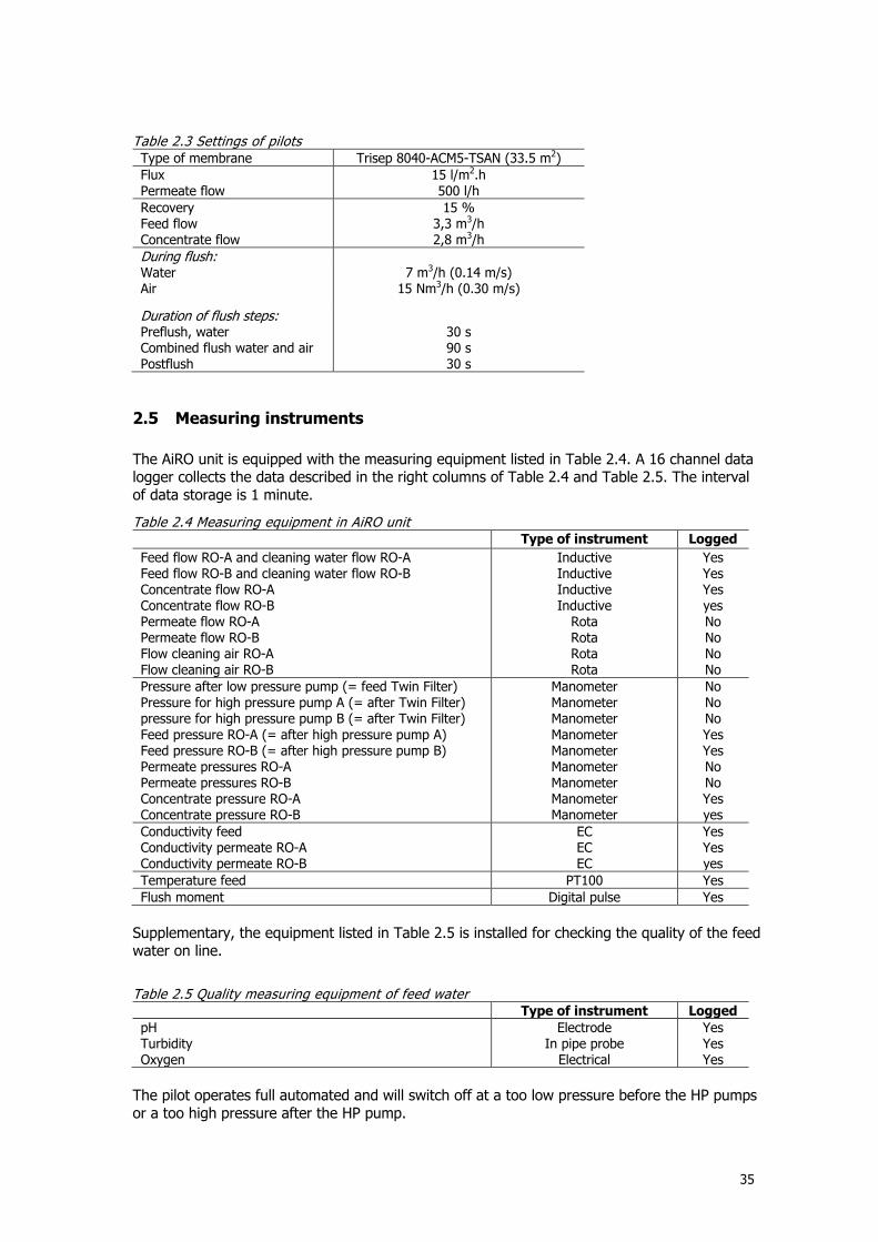
2.5 Measuring instruments

The AiRO unit is equipped with the measuring equipment listed in Table 2.4. A 16 channel data logger collects the data described in the right columns of Table 2.4 and Table 2.5. The interval of data storage is 1 minute.

Table 2.4 Measuring equipment in AiRO unit

Type of instrument Logged

Feed flow RO-A and cleaning water flow RO-A Feed flow RO-B and cleaning water flow RO-B Concentrate flow RO-A Concentrate flow RO-B Permeate flow RO-A Permeate flow RO-B Flow cleaning air RO-A Flow cleaning air RO-B

Inductive Inductive Inductive Inductive

Rota Rota Rota Rota

Yes Yes Yes yes No No No No

Pressure after low pressure pump (= feed Twin Filter) Pressure for high pressure pump A (= after Twin Filter) pressure for high pressure pump B (= after Twin Filter) Feed pressure RO-A (= after high pressure pump A) Feed pressure RO-B (= after high pressure pump B) Permeate pressures RO-A Permeate pressures RO-B Concentrate pressure RO-A Concentrate pressure RO-B

Manometer Manometer Manometer Manometer Manometer Manometer Manometer Manometer Manometer

No No No Yes Yes No No Yes yes

Conductivity feed Conductivity permeate RO-A Conductivity permeate RO-B

EC EC EC

Yes Yes yes

Temperature feed PT100 Yes

Flush moment Digital pulse Yes

Supplementary, the equipment listed in Table 2.5 is installed for checking the quality of the feed water on line.

Table 2.5 Quality measuring equipment of feed water Type of instrument Logged pH Turbidity Oxygen

Electrode In pipe probe

Electrical

Yes Yes Yes

The pilot operates full automated and will switch off at a too low pressure before the HP pumps or a too high pressure after the HP pump.

36

2.6 Sample programme

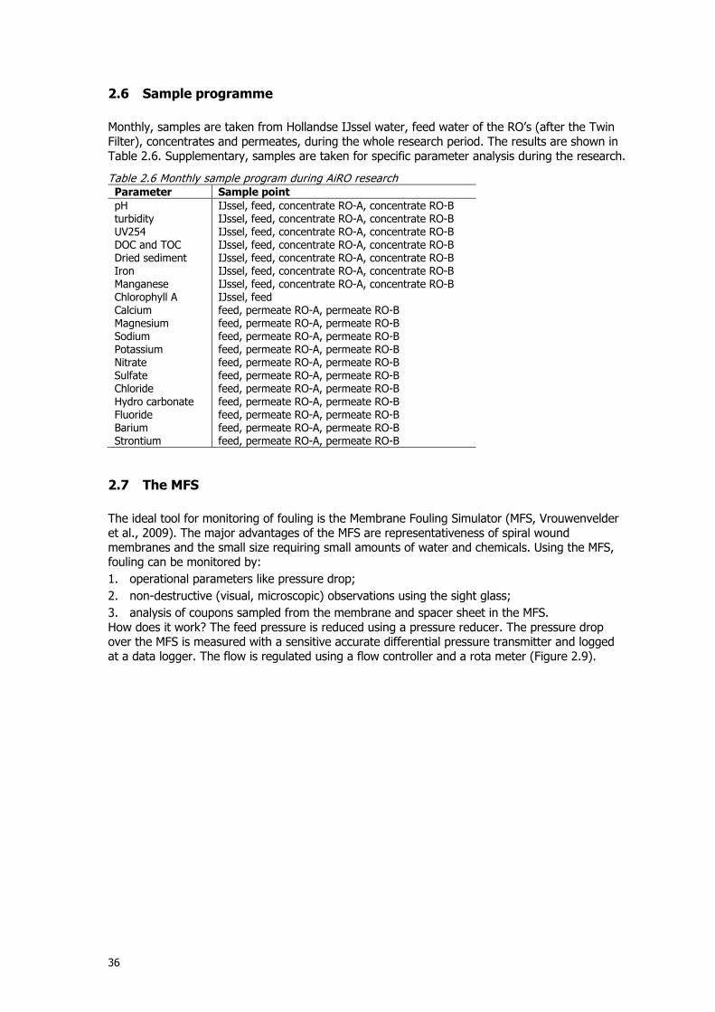
Monthly, samples are taken from Hollandse IJssel water, feed water of the RO’s (after the Twin Filter), concentrates and permeates, during the whole research period. The results are shown in Table 2.6. Supplementary, samples are taken for specific parameter analysis during the research.

Table 2.6 Monthly sample program during AiRO research Parameter Sample point

pH turbidity UV254 DOC and TOC Dried sediment Iron Manganese Chlorophyll A Calcium Magnesium Sodium Potassium Nitrate Sulfate Chloride Hydro carbonate Fluoride Barium Strontium

IJssel, feed, concentrate RO-A, concentrate RO-B IJssel, feed, concentrate RO-A, concentrate RO-B IJssel, feed, concentrate RO-A, concentrate RO-B IJssel, feed, concentrate RO-A, concentrate RO-B IJssel, feed, concentrate RO-A, concentrate RO-B IJssel, feed, concentrate RO-A, concentrate RO-B IJssel, feed, concentrate RO-A, concentrate RO-B IJssel, feed feed, permeate RO-A, permeate RO-B feed, permeate RO-A, permeate RO-B feed, permeate RO-A, permeate RO-B feed, permeate RO-A, permeate RO-B feed, permeate RO-A, permeate RO-B feed, permeate RO-A, permeate RO-B feed, permeate RO-A, permeate RO-B feed, permeate RO-A, permeate RO-B feed, permeate RO-A, permeate RO-B feed, permeate RO-A, permeate RO-B feed, permeate RO-A, permeate RO-B

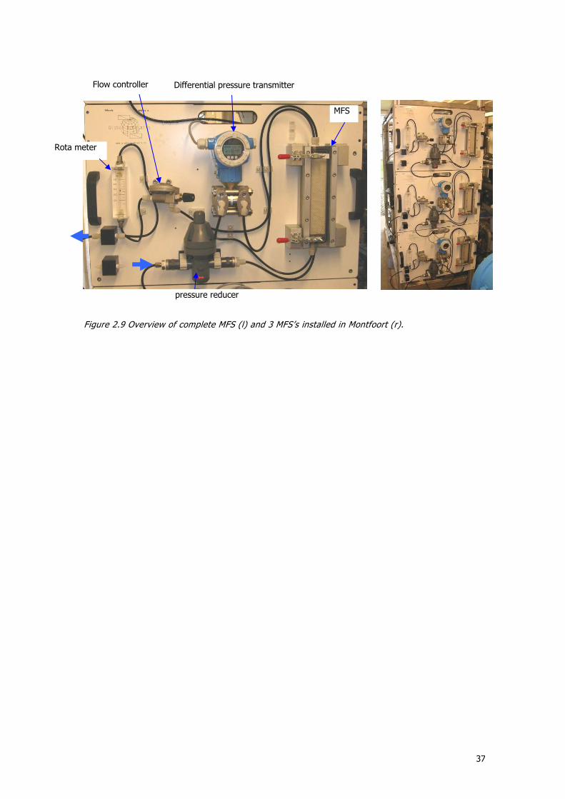
2.7 The MFS

The ideal tool for monitoring of fouling is the Membrane Fouling Simulator (MFS, Vrouwenvelder et al., 2009). The major advantages of the MFS are representativeness of spiral wound membranes and the small size requiring small amounts of water and chemicals. Using the MFS, fouling can be monitored by:

1. operational parameters like pressure drop;

2. non-destructive (visual, microscopic) observations using the sight glass;

3. analysis of coupons sampled from the membrane and spacer sheet in the MFS. How does it work? The feed pressure is reduced using a pressure reducer. The pressure drop over the MFS is measured with a sensitive accurate differential pressure transmitter and logged at a data logger. The flow is regulated using a flow controller and a rota meter (Figure 2.9).

37

Differential pressure transmitter

Rota meter

Flow controller

pressure reducer

MFS

Figure 2.9 Overview of complete MFS (l) and 3 MFS’s installed in Montfoort (r).

38

3 Results

In this chapter the results of the AiRO research will be handled. Main line in the text will be the aim of the objectives that are described in § 1.8. The chapter will start with a brief overview of the executed research in Montfoort.

3.1 Overview of results of pilot research Montfoort

The AiRO research in Montfoort begun on Monday December 27th 2010 and finished on July 17th 2012. During those 568 days, the pilot and the peripheral equipment operated reliable. No serious technical incidents have been observed, except some standstill time, which was caused by fouling of the Twin Filter. During this AiRO research, in each pilot subsequent 2 membrane elements are tested. The first set of elements was used to evolve a sufficient flush interval and to determine the flush program. For the second period new and non fouled membrane modules were installed and research took place with an almost fixed flush procedure and fixed operational settings (Table 2.3). The operation of the pilots in both periods is examined by means of the calculated mass transfer coefficient (MTC), normalized pressure drop (NPD) and normalized salt passage (NSP). Those parameters and the calculation methods are explained in annex 1. In annex 5 the MTC, NPD and NSP in the whole first period (figure 1) and second period (figure 2) are shown. It’s not possible yet to draw any conclusions out of those graphs, the data will be analysed by answering the objectives of the research.

3.1.1 Applied pretreatment during AiRO research

Surface water has been applied as source water without pre treatment before the AiRO membrane (Hippönen, 2009). The feed water contains particles of different sizes. Particles that can’t pass the membrane feed spacer have to be removed from the surface water, to protect the membrane spacer and thus element from blocking. The smallest spacer thickness in Montfoort was 0.7 mm. A spacer is constructed of two crossed linked filaments with a thickness of half of the total spacer thickness. The opening between the membrane and filament is 0.7 mm/2 = 0.35 mm. This means that particles larger than 0.35 mm can’t pass the openings between spacer and membrane surface. The smallest bore of the applied pre treatment in Montfoort is the drumfilter with of a mesh of 120 µm. The biggest particles that pass through this drum filter are about 3 times smaller than the openings in the feed spacer. So the biggest particles that can pas the drumfilter can move through the openings in the spacer. If a large amount of particles is stopped in the drumfilter, there should be a significant difference in particles content between feedwater and filtrate. This can be observed with the amount of SS, turbidity and iron in those water flows. In Table 3.1 the percentile removal of turbidity and iron in the drum filter is summarized (SS is not analysed in feed of drumfilter). The numbers are based on the monthly taken samples from Hollandse IJssel river water and from feed RO.

Table 3.1 Removal of turbidity and iron in drumfilter. Positive numbers indicate a removal.

Influent average

Effluent average

Removal

Average Minimum Maximum Std

Turbidity [FTU] 15.5 15.1 3 % -18 % 14 % 9

Iron [mg/l Fe] 1.0 1.0 -1 % -8 % 15 % 6

The variation in removal is large, in some situations turbidity and iron are removed in the drumfilter but in the same amount of situations they are larger after the filter than before it. The accuracy of the analysis and method of sampling seems to introduce variation, according the large standard deviation. A significant effect of the drumfilter on turbidity and iron and thus particles is not observed.

39

For this reason is concluded that the drumfilter influences the size of the particles, not the load. The particles in the feed of the RO’s are in size smaller than the drumfilter mesh of 0.12 mm.

3.1.2 Steps of flush of the AiRO process?

In literature only the air/water flush (combined flush) is described. Goal of the flush procedure is to remove trapped particles and biological debris. But is just a combined step sufficient for this purpose and does a flush have more functions? A in the Montfoort research founded idea is that there is consistence between a rapid sand filter and a vertical placed AiRO membrane element. A rapid sand filter backwash procedure consists of 3 steps; a preflush step with water only, a combined flush step with water and air and a postflush step with water only. Goal of those flush steps in a rapid sand filter are: Preflush removes loose debris from the top of the filter material; Combined flush releases attached debris from the sand and transports it out of the filter Postflush removes loosened debris from the filter and releases flush air from the sand. This idea is applied on the AiRO process in this research. The function of the steps in the AiRO research was: Function of preflush: Goal of the preflush is to wash out the non fixed part of the filtered suspended solids before the combined flush takes place. In this step will only wash out the debris that is not tight fixed to the membrane or spacer. Function of air/water flush: The (bio)fouling deposited on the feed spacer and membrane is released and removed with an upflow air/water flush, in fact the combined flush of a rapid sand filter. Function of postflush: One goal of the postflush is to wash out the solids that are released during the combined flush and are not dispatched yet. The other goal is to wash out the air bubbles that might be trapped in the spacer or somewhere else in the pressure vessel after the combined flush. After a flush at low pressure, the pilot is pressurized again by means of the high pressure pump and put back in operation. If still air is present in the pressure vessel, air bubbles at high pressure might damage the concentrate control valve (cavitation). A flush program containing those three steps is applied during the whole AiRO research in Montfoort.

3.2 What will be the duration of the defined flush steps?

Now the individual steps of the flush are known, but what will be the duration of the individual steps of it? The duration of the combined flush is between 5 and 60 minutes as described in literature (Table 1.4). The duration of pre- and postflush is not mentioned in literature and have to be studied from scratch. Duration of the three flush steps during the AiRO research is summarized in Table 3.2.

Table 3.2 Band with in duration of flush steps in Montfoort

Flush setting Minimum Maximum

Pre water flush [s] Combined flush [s] Post water flush [s]

15 1

30 15 2

30 180 30

1 applied during 43 days and changed to 30 s 2 applied during 2 days and changed to 30 s

After a half year of operation a fixed flush procedure is determined. This determination is described in this paragraph. First the duration of the pre- and postflush will be described.

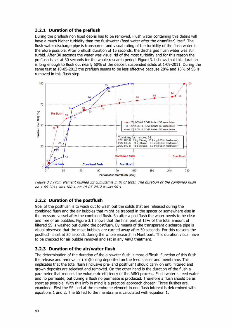
40

3.2.1 Duration of the preflush

During the preflush non fixed debris has to be removed. Flush water containing this debris will have a much higher turbidity than the flushwater (feed water after the drumfilter) itself. The flush water discharge pipe is transparent and visual rating of the turbidity of the flush water is therefore possible. After preflush duration of 15 seconds, the discharged flush water was still turbid. After 30 seconds the water was visual rid of the most turbidity and for this reason the preflush is set at 30 seconds for the whole research period. Figure 3.1 shows that this duration is long enough to flush out nearly 50% of the deposit suspended solids at 1-09-2011. During the same test at 10-05-2012 the preflush seems to be less effective because 28% and 13% of SS is removed in this flush step.

3.2.2 Duration of the postflush

Goal of the postflush is to wash out to wash out the solids that are released during the combined flush and the air bubbles that might be trapped in the spacer or somewhere else in the pressure vessel after the combined flush. So after a postflush the water needs to be clear and free of air bubbles. Figure 3.1 shows that the final part of 15% of the total amount of filtered SS is washed out during the postflush. By means of the transparent discharge pipe is visual observed that the most bubbles are carried away after 30 seconds. For this reasons the postflush is set at 30 seconds during the whole research in Montfoort. This duration visual have to be checked for air bubble removal and set in any AiRO treatment.

3.2.3 Duration of the air/water flush

The determination of the duration of the air/water flush is more difficult. Function of this flush the release and removal of (bio)fouling deposited on the feed spacer and membrane. This implicates that the total flush (inclusive pre- and postflush) should carry on until filtered and grown deposits are released and removed. On the other hand is the duration of the flush a parameter that reduces the volumetric efficiency of the AiRO process. Flush water is feed water and no permeate, but during a flush no permeate is produced. Therefore a flush should be as short as possible. With this info in mind is a practical approach chosen. Three flushes are examined. First the SS load at the membrane element in one flush interval is determined with equations 1 and 2. The SS fed to the membrane is calculated with equation 1:

Figure 3.1 From element flushed SS cumulative in % of total. The duration of the combined flush

on 1-09-2011 was 180 s, on 10-05-2012 it was 90 s.

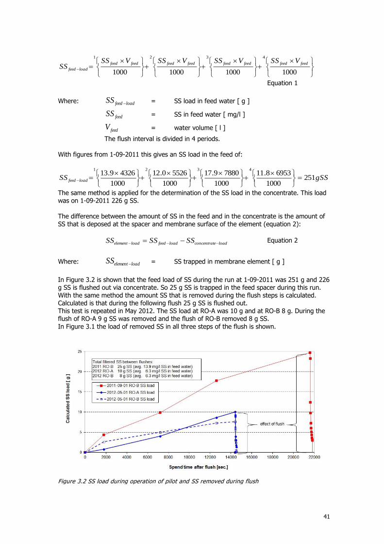
41

1000100010001000

4321

feedfeedfeedfeedfeedfeedfeedfeed

loadfeed

VSSVSSVSSVSSSS

Equation 1

Where: loadfeedSS = SS load in feed water [ g ]

feedSS = SS in feed water [ mg/l ]

feedV = water volume [ l ]

The flush interval is divided in 4 periods. With figures from 1-09-2011 this gives an SS load in the feed of:

gSSSS loadfeed 2511000

69538.11

1000

78809.17

1000

55260.12

1000

43269.134321

The same method is applied for the determination of the SS load in the concentrate. This load was on 1-09-2011 226 g SS. The difference between the amount of SS in the feed and in the concentrate is the amount of SS that is deposed at the spacer and membrane surface of the element (equation 2):

loadeconcentratloadfeedloadelement SSSSSS Equation 2

Where: loadelementSS = SS trapped in membrane element [ g ]

In Figure 3.2 is shown that the feed load of SS during the run at 1-09-2011 was 251 g and 226 g SS is flushed out via concentrate. So 25 g SS is trapped in the feed spacer during this run. With the same method the amount SS that is removed during the flush steps is calculated. Calculated is that during the following flush 25 g SS is flushed out. This test is repeated in May 2012. The SS load at RO-A was 10 g and at RO-B 8 g. During the flush of RO-A 9 g SS was removed and the flush of RO-B removed 8 g SS. In Figure 3.1 the load of removed SS in all three steps of the flush is shown.

Figure 3.2 SS load during operation of pilot and SS removed during flush

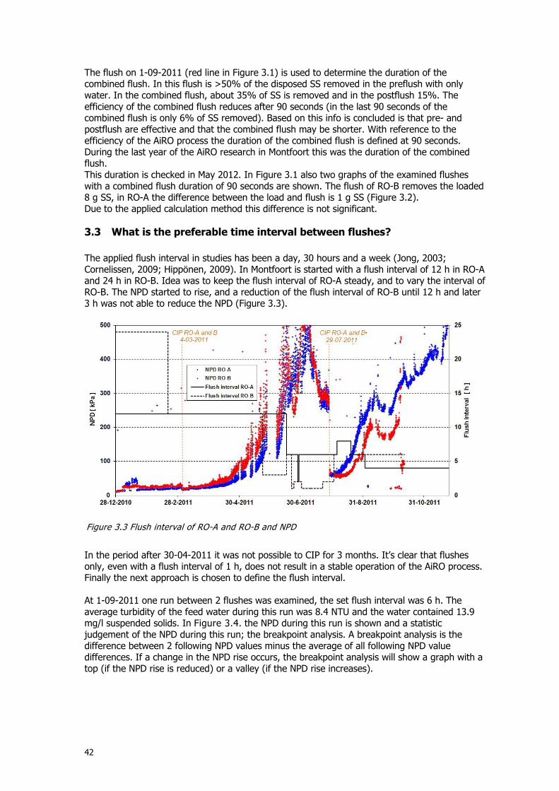
42

The flush on 1-09-2011 (red line in Figure 3.1) is used to determine the duration of the combined flush. In this flush is >50% of the disposed SS removed in the preflush with only water. In the combined flush, about 35% of SS is removed and in the postflush 15%. The efficiency of the combined flush reduces after 90 seconds (in the last 90 seconds of the combined flush is only 6% of SS removed). Based on this info is concluded is that pre- and postflush are effective and that the combined flush may be shorter. With reference to the efficiency of the AiRO process the duration of the combined flush is defined at 90 seconds. During the last year of the AiRO research in Montfoort this was the duration of the combined flush. This duration is checked in May 2012. In Figure 3.1 also two graphs of the examined flushes with a combined flush duration of 90 seconds are shown. The flush of RO-B removes the loaded 8 g SS, in RO-A the difference between the load and flush is 1 g SS (Figure 3.2). Due to the applied calculation method this difference is not significant.

3.3 What is the preferable time interval between flushes?

The applied flush interval in studies has been a day, 30 hours and a week (Jong, 2003; Cornelissen, 2009; Hippönen, 2009). In Montfoort is started with a flush interval of 12 h in RO-A and 24 h in RO-B. Idea was to keep the flush interval of RO-A steady, and to vary the interval of RO-B. The NPD started to rise, and a reduction of the flush interval of RO-B until 12 h and later 3 h was not able to reduce the NPD (Figure 3.3).

In the period after 30-04-2011 it was not possible to CIP for 3 months. It’s clear that flushes only, even with a flush interval of 1 h, does not result in a stable operation of the AiRO process. Finally the next approach is chosen to define the flush interval. At 1-09-2011 one run between 2 flushes was examined, the set flush interval was 6 h. The average turbidity of the feed water during this run was 8.4 NTU and the water contained 13.9 mg/l suspended solids. In Figure 3.4. the NPD during this run is shown and a statistic judgement of the NPD during this run; the breakpoint analysis. A breakpoint analysis is the difference between 2 following NPD values minus the average of all following NPD value differences. If a change in the NPD rise occurs, the breakpoint analysis will show a graph with a top (if the NPD rise is reduced) or a valley (if the NPD rise increases).

Figure 3.3 Flush interval of RO-A and RO-B and NPD

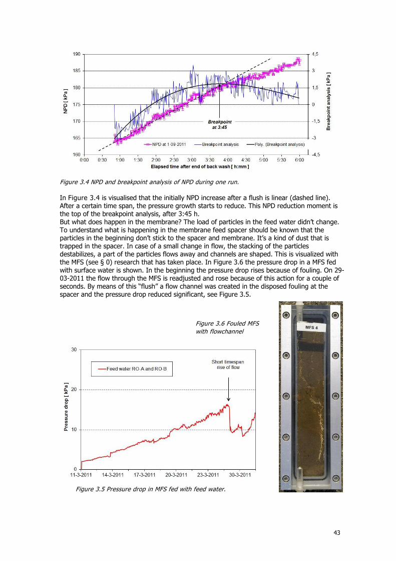
43

Figure 3.4 NPD and breakpoint analysis of NPD during one run.

In Figure 3.4 is visualised that the initially NPD increase after a flush is linear (dashed line). After a certain time span, the pressure growth starts to reduce. This NPD reduction moment is the top of the breakpoint analysis, after 3:45 h. But what does happen in the membrane? The load of particles in the feed water didn’t change. To understand what is happening in the membrane feed spacer should be known that the particles in the beginning don’t stick to the spacer and membrane. It’s a kind of dust that is trapped in the spacer. In case of a small change in flow, the stacking of the particles destabilizes, a part of the particles flows away and channels are shaped. This is visualized with the MFS (see § 0) research that has taken place. In Figure 3.6 the pressure drop in a MFS fed with surface water is shown. In the beginning the pressure drop rises because of fouling. On 29-03-2011 the flow through the MFS is readjusted and rose because of this action for a couple of seconds. By means of this “flush” a flow channel was created in the disposed fouling at the spacer and the pressure drop reduced significant, see Figure 3.5.

Figure 3.5 Pressure drop in MFS fed with feed water.

Figure 3.6 Fouled MFS

with flowchannel

44

This is an undesirable situation, because the water velocity at a part of the membrane will be reduced and the concentration polarisation will rise. This will result in unwanted scaling at the membrane surface. So in the AiRO membrane element initially particles block parts of the spacer, but water is still able to flow though the entire spacer. At a certain moment the NPD does raise less fast. From this moment flow channels are formed like in the MFS. This is an undesirable situation, because it costs flush time and flush energy to overcome the disadvantages of this channelling. In Figure 3.4 can be observed that the breakpoint is situated just before the 4 h. After 1-09-2011 the flush interval in the Montfoort research was determined for this reason on 4 h.

3.4 What will be the water and air velocity during flush?

During the flush steps, air and/or water is pressed through the feed spacer to remove debris from it and from the membrane surface. In literature, it is described that the velocity of air and water during the combined flush varied between respectively 0.04-2.4 m/s and 0.09-0.8 m/s (Table 1.4). With 0.4 m/s of water the area coverage of the air bubbles is sufficient (Willems, 2009) and a Reynolds number greater than 140 gives turbid flow in a membrane spacer (Shakaib, 2007). During the AiRO research on surface water in Montfoort the RO’s are flushed at set times with water and air, which is the basic principle of AiRO. The flush intensity is not calculated before the experiments in Montfoort. A practical approach is chosen, during a trail period with the first set of membrane elements, the band width of the applied flush procedure is determined. The aim of this paragraph is the determination of the optimal flush intensity of the AiRO process. In one timespan in the second period, the intensity of the flush in RO-A and B was different. The period and the settings are shown in Table 3.3.

Table 3.3 Differentiated setting of pilots during the AiRO research Period Process difference

Start End RO-A RO-B

Intensity of flush steps

Preflush water Combined flush water Combined flush air Postflush water

26-03- 2012

10-05- 2012

7 m3/h (0.14 m/s) 5.5 m3/h (0.11 m/s)

15 Nm3/h (0.30 Nm/s) 7 m3/h (0.14 m/s)

10 m3/h (0.20 m/s) 7.8 m3/h (0.16 m/s)

18 Nm3/h (0.36 Nm/s) 10 m3/h (0.20 m/s)

This period mentioned in Table 3.3 is used for the determination of the intensity of the flushes and for the determination of the influence of different flush intensities.

3.4.1 Determination of intensity of flush steps

To estimate the intensity of a total flush, the intensity of the parts of a flush has to be known. This means the intensity of both water flushes and of the combined flush. A common used parameter to describe the water turbulence is the Reynolds number. Reynolds numbers frequently arise when performing fluid dynamics problems, which can be used to determine dynamic similitude between two different cases of fluid flow. They are also used to characterize different flow regimes within a similar fluid, such as laminar or turbulent flow: laminar flow occurs at low Reynolds numbers and is characterized by smooth, constant fluid motion; turbulent flow occurs at high Reynolds numbers, see Figure 3.7.

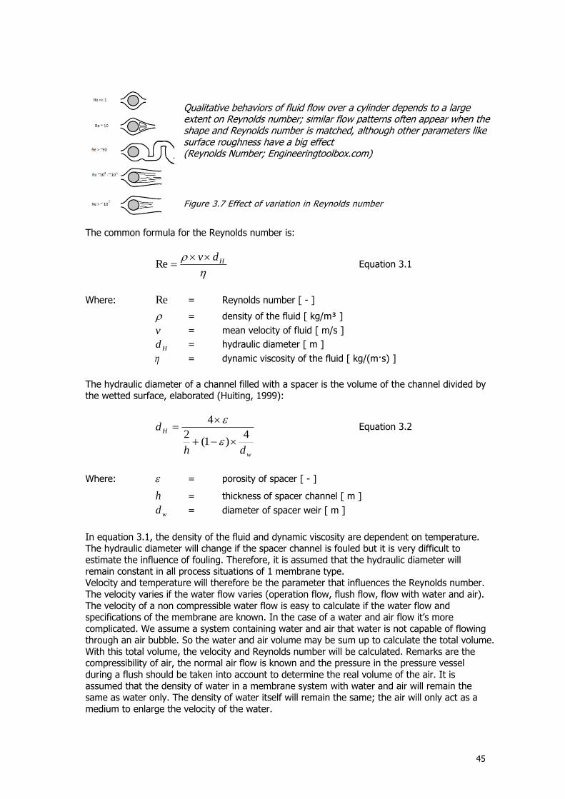
45

Qualitative behaviors of fluid flow over a cylinder depends to a large extent on Reynolds number; similar flow patterns often appear when the shape and Reynolds number is matched, although other parameters like surface roughness have a big effect (Reynolds Number; Engineeringtoolbox.com)

The common formula for the Reynolds number is:

HdvRe Equation 3.1

Where: Re = Reynolds number [ - ]

= density of the fluid [ kg/m³ ]

v = mean velocity of fluid [ m/s ]

Hd = hydraulic diameter [ m ]

= dynamic viscosity of the fluid [ kg/(m·s) ]

The hydraulic diameter of a channel filled with a spacer is the volume of the channel divided by the wetted surface, elaborated (Huiting, 1999):

w

H

dh

d4

)1(2

4

Equation 3.2

Where: = porosity of spacer [ - ]

h = thickness of spacer channel [ m ]

wd = diameter of spacer weir [ m ]

In equation 3.1, the density of the fluid and dynamic viscosity are dependent on temperature. The hydraulic diameter will change if the spacer channel is fouled but it is very difficult to estimate the influence of fouling. Therefore, it is assumed that the hydraulic diameter will remain constant in all process situations of 1 membrane type. Velocity and temperature will therefore be the parameter that influences the Reynolds number. The velocity varies if the water flow varies (operation flow, flush flow, flow with water and air). The velocity of a non compressible water flow is easy to calculate if the water flow and specifications of the membrane are known. In the case of a water and air flow it’s more complicated. We assume a system containing water and air that water is not capable of flowing through an air bubble. So the water and air volume may be sum up to calculate the total volume. With this total volume, the velocity and Reynolds number will be calculated. Remarks are the compressibility of air, the normal air flow is known and the pressure in the pressure vessel during a flush should be taken into account to determine the real volume of the air. It is assumed that the density of water in a membrane system with water and air will remain the same as water only. The density of water itself will remain the same; the air will only act as a medium to enlarge the velocity of the water.

Figure 3.7 Effect of variation in Reynolds number

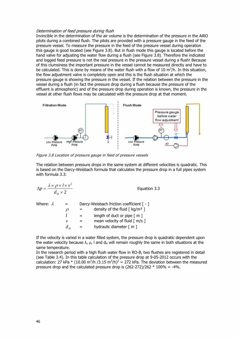
46

Determination of feed pressure during flush Invincible in the determination of the air volume is the determination of the pressure in the AiRO pilots during a combined flush. The pilots are provided with a pressure gauge in the feed of the pressure vessel. To measure the pressure in the feed of the pressure vessel during operation this gauge is good located (see Figure 3.8). But in flush mode this gauge is located before the hand valve for adjusting the water flow during a flush (see Figure 3.8). Therefore the indicated and logged feed pressure is not the real pressure in the pressure vessel during a flush! Because of this clumsiness the important pressure in the vessel cannot be measured directly and have to be calculated. This is done by means of the water flush with a flow of 10 m3/h. In this situation, the flow adjustment valve is completely open and this is the flush situation at which the pressure gauge is showing the pressure in the vessel. If the relation between the pressure in the vessel during a flush (in fact the pressure drop during a flush because the pressure of the effluent is atmospheric) and of the pressure drop during operation is known, the pressure in the vessel at other flush flows may be calculated with the pressure drop at that moment.

Figure 3.8 Location of pressure gauge in feed of pressure vessels

The relation between pressure drops in the same system at different velocities is quadratic. This is based on the Darcy-Weisbach formula that calculates the pressure drop in a full pipes system with formula 3.3:

2

2

Hd

vlp

Equation 3.3

Where: = Darcy-Weisbach friction coefficient [ - ]

= density of the fluid [ kg/m³ ]

l = length of duct or pipe [ m ]

v = mean velocity of fluid [ m/s ]

Hd = hydraulic diameter [ m ]

If the velocity is varied in a water filled system, the pressure drop is quadratic dependent upon the water velocity because λ, ρ, l and dH will remain roughly the same in both situations at the

same temperature. In the research period with a high flush water flow in RO-B, two flushes are registered in detail (see Table 3.4). In this table calculation of the pressure drop at 9-05-2012 occurs with the calculation: 27 kPa * (10.00 m3/h /3.15 m3/h)2 = 272 kPa. The deviation between the measured pressure drop and the calculated pressure drop is (262-272)/262 * 100% = -4%.

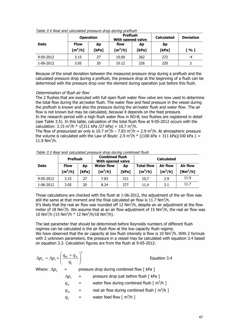
47

Table 3.4 Real and calculated pressure drop during preflush

Operation

Preflush With opened valve

Calculated Deviation

Date Flow Δp flow Δp Δp

[m3/h] [kPa] [m3/h] [kPa] [kPa] [ % ]

9-05-2012 3.15 27 10.00 262 272 -4

1-06-2012 3.05 20 10.12 226 220 3

Because of the small deviation between the measured pressure drop during a preflush and the calculated pressure drop during a preflush, the pressure drop at the beginning of a flush can be determined with the pressure drop over the element during operation just before this flush. Determination of flush air flow The 2 flushes that are executed with full open flush water flow valve are now used to determine the total flow during the air/water flush. The water flow and feed pressure in the vessel during the preflush is known and also the pressure during the air/water flush and water flow. The air flow is not known but may be calculated, because it depends on the feed pressure. In the research period with a high flush water flow in RO-B, two flushes are registered in detail (see Table 3.5). In this table, calculation of the total flush flow at 9-05-2012 occurs with the calculation: 3.15 m3/h * √(311 kPa /27 kPa) = 10.7 m3/h. The flow of pressurized air only is 10.7 m3/h – 7.83 m3/h = 2.9 m3/h. At atmospheric pressure the volume is calculated with the Law of Boyle: 2.9 m3/h * {(100 kPa + 311 kPa)/100 kPa } = 11.9 Nm3/h.

Table 3.5 Real and calculated pressure drop during combined flush

Preflush

Combined flush With opened valve

Calculated

Date Flow Δp Water flow Δp Total flow Air flow Air flow

[m3/h] [kPa] [m3/h] [kPa] [m3/h] [m3/h] [Nm3/h]

9-05-2012 3.15 27 7.83 311 10,7 2.9 11.9

1-06-2012 3.05 20 8.24 277 11,4 3.1 11.7

Those calculations are checked with the flush at 1-06-2012, the adjustment of the air flow was still the same at that moment and the final calculated air flow is 11.7 Nm3/h. It’s likely that the real air flow was rounded off 12 Nm3/h, despite an air adjustment at the flow meter of 18 Nm3/h. We assume that at an air flow adjustment of 15 Nm3/h, the real air flow was 10 Nm3/h (15 Nm3/h * 12 Nm3/h/18 Nm3/h). The last parameter that should be determined before Reynolds numbers of different flush regimes can be calculated is the air flush flow at the low capacity flush regime. We have observed that the air capacity at low flush intensity is flow is 10 Nm3/h. With 2 formula with 2 unknown parameters, the pressure in a vessel may be calculated with equation 3.4 based on equation 3.3. Calculation figures are from the flush at 9-05-2012:

2

1

1

q

qqpp AW

C Equation 3.4

Where: Cp = pressure drop during combined flow [ kPa ]

1p = pressure drop just before flush [ kPa ]

wq = water flow during combined flush [ m3/h ]

Aq = real air flow during combined flush [ m3/h ]

1q = water feed flow [ m3/h ]

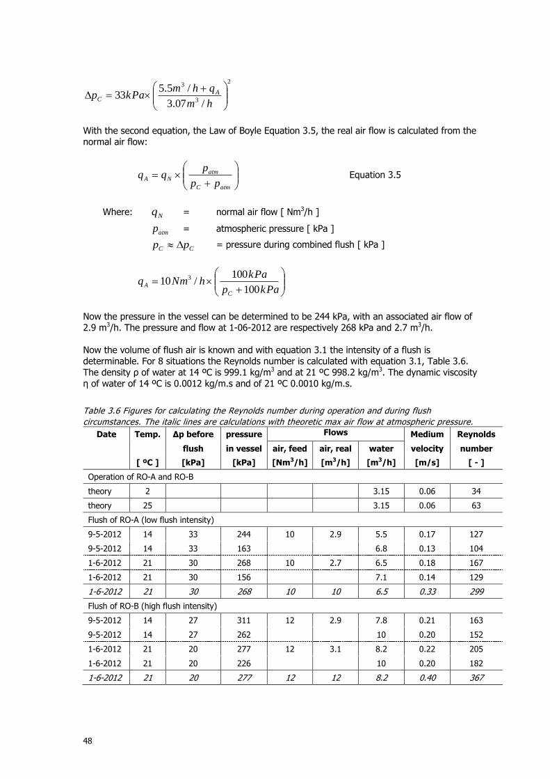
48

2

3

3

/07.3

/5.533

hm

qhmkPap A

C

With the second equation, the Law of Boyle Equation 3.5, the real air flow is calculated from the normal air flow:

atmC

atmNA

pp

pqq Equation 3.5

Where: Nq = normal air flow [ Nm3/h ]

atmp = atmospheric pressure [ kPa ]

CC pp = pressure during combined flush [ kPa ]

kPap

kPahNmq

C

A100

100/10 3

Now the pressure in the vessel can be determined to be 244 kPa, with an associated air flow of 2.9 m3/h. The pressure and flow at 1-06-2012 are respectively 268 kPa and 2.7 m3/h. Now the volume of flush air is known and with equation 3.1 the intensity of a flush is determinable. For 8 situations the Reynolds number is calculated with equation 3.1, Table 3.6. The density ρ of water at 14 ºC is 999.1 kg/m3 and at 21 ºC 998.2 kg/m3. The dynamic viscosity η of water of 14 ºC is 0.0012 kg/m.s and of 21 ºC 0.0010 kg/m.s.

Table 3.6 Figures for calculating the Reynolds number during operation and during flush

circumstances. The italic lines are calculations with theoretic max air flow at atmospheric pressure.

Date Temp. Δp before pressure Flows Medium Reynolds

flush in vessel air, feed air, real water velocity number

[ ºC ] [kPa] [kPa] [Nm3/h] [m3/h] [m3/h] [m/s] [ - ]

Operation of RO-A and RO-B

theory 2 3.15 0.06 34

theory 25 3.15 0.06 63

Flush of RO-A (low flush intensity)

9-5-2012 14 33 244 10 2.9 5.5 0.17 127

9-5-2012 14 33 163

6.8 0.13 104

1-6-2012 21 30 268 10 2.7 6.5 0.18 167

1-6-2012 21 30 156

7.1 0.14 129

1-6-2012 21 30 268 10 10 6.5 0.33 299

Flush of RO-B (high flush intensity)

9-5-2012 14 27 311 12 2.9 7.8 0.21 163

9-5-2012 14 27 262

10 0.20 152

1-6-2012 21 20 277 12 3.1 8.2 0.22 205

1-6-2012 21 20 226

10 0.20 182

1-6-2012 21 20 277 12 12 8.2 0.40 367

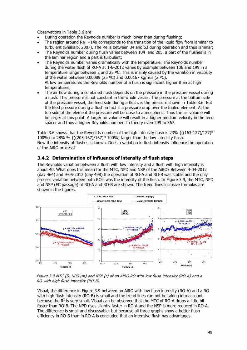
49

Observations in Table 3.6 are: During operation the Reynolds number is much lower than during flushing; The region around ReL ∼140 corresponds to the transition of the liquid flow from laminar to

turbulent (Shakaib, 2007). The Re is between 34 and 63 during operation and thus laminar; The Reynolds number during flush varies between 104 and 205, a part of the flushes is in

the laminar region and a part is turbulent; The Reynolds number varies dramatically with the temperature. The Reynolds number

during the water flush of RO-A at 1-6-2012 varies by example between 106 and 199 in a temperature range between 2 and 25 ºC. This is mainly caused by the variation in viscosity of the water between 0.00089 (25 ºC) and 0.00167 kg/m.s (2 ºC). At low temperatures the Reynolds number of a flush is significant higher than at high temperatures;

The air flow during a combined flush depends on the pressure in the pressure vessel during a flush. This pressure is not constant in the whole vessel. The pressure at the bottom side of the pressure vessel, the feed side during a flush, is the pressure shown in Table 3.6. But the feed pressure during a flush in fact is a pressure drop over the fouled element. At the top side of the element the pressure will be close to atmospheric. Thus the air volume will be larger at this point. A larger air volume will result in a higher medium velocity in the feed spacer and thus a higher Reynolds number. In theory even 299 to 367.

Table 3.6 shows that the Reynolds number of the high intensity flush is 23% {((163-127)/127)* 100%} to 28% % {((205-167)/167)* 100%} larger than the low intensity flush. Now the intensity of flushes is known. Does a variation in flush intensity influence the operation of the AiRO process?

3.4.2 Determination of influence of intensity of flush steps

The Reynolds variation between a flush with low intensity and a flush with high intensity is about 40. What does this mean for the MTC, NPD and NSP of the AiRO? Between 4-04-2012 (day 464) and 9-05-2012 (day 498) the operation of RO-A and RO-B was stable and the only process variation between both RO’s was the intensity of the flush. In Figure 3.9, the MTC, NPD and NSP (EC passage) of RO-A and RO-B are shown. The trend lines inclusive formulas are shown in the figures.

Visual, the difference in Figure 3.9 between an AiRO with low flush intensity (RO-A) and a RO with high flush intensity (RO-B) is small and the trend lines can not be taking into account because the R2 is very small. Visual can be observed that the MTC of RO-A drops a little bit faster than RO-B. The NPD rises slightly faster in RO-A and the NSP is more reduced in RO-A. The difference is small and discussable, but because all three graphs show a better flush efficiency in RO-B than in RO-A is concluded that an intensive flush has advantages.

Figure 3.9 MTC (l), NPD (m) and NSP (r) of an AiRO RO with low flush intensity (RO-A) and a

RO with high flush intensity (RO-B).

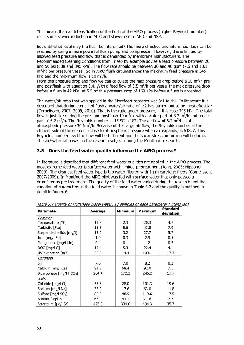
50

This means than an intensification of the flush of the AiRO process (higher Reynolds number) results in a slower reduction in MTC and slower rise of NPD and NSP. But until what level may the flush be intensified? The more effective and intensified flush can be reached by using a more powerful flush pump and compressor. However, this is limited by allowed feed pressure and flow that is demanded by membrane manufacturers. The Recommended Cleaning Conditions from Trisep by example advise a feed pressure between 20 and 50 psi (138 and 345 kPa). The flow rate should be between 30 and 40 gpm (7.6 and 10.1 m3/h) per pressure vessel. So in AiRO flush circumstances the maximum feed pressure is 345 kPa and the maximum flow is 10 m3/h. From this pressure drop and flow we can calculate the max pressure drop before a 10 m3/h pre- and postflush with equation 3.4. With a feed flow of 3.5 m3/h per vessel the max pressure drop before a flush is 42 kPa, at 5.5 m3/h a pressure drop of 169 kPa before a flush is accepted. The water/air ratio that was applied in the Montfoort research was 3:1 to 4:1. In literature it is described that during combined flush a water/air ratio of 1:2 has turned out to be most effective (Cornelissen, 2007, 2009, 2010). That is the ratio under pressure, in this case 345 kPa. The total flow is just like during the pre- and postflush 10 m3/h, with a water part of 3.3 m3/h and an air part of 6.7 m3/h. The Reynolds number at 15 ºC is 187. The air flow of 6.7 m3/h is at atmospheric pressure 30 Nm3/h. Because of this large air flow, the Reynolds number at the effluent side of the element (close to atmospheric pressure when air expands) is 618. At this Reynolds number level the flow will be turbulent and the shear stress on fouling will be large. The air/water ratio was no the research subject during the Montfoort research.

3.5 Does the feed water quality influence the AiRO process?

In literature is described that different feed water qualities are applied in the AiRO process. The most extreme feed water is surface water with limited pretreatment (Jong, 2003; Hippönen, 2009). The cleanest feed water type is tap water filtered with 1 µm cartridge filters (Cornelissen, 2007/2009). In Montfoort the AiRO pilot was fed with surface water that only passed a drumfilter as pre treatment. The quality of the feed water varied during the research and the variation of parameters in the feed water is shown in Table 3.7 and the quality is outlined in detail in Annex 6.

Table 3.7 Quality of Hollandse IJssel water, 13 samples of each parameter (Vitens lab)

Parameter Average Minimum Maximum Standard deviation

Common Temperature [°C] 11.3 2.3 20.3 4.7

Turbidity [Ftu] 15.5 5.6 43.8 7.9

Suspended solids [mg/l] 13.0 3.2 27.7 5.7

Iron [mg/l Fe] 1.0 0.3 2.9 0.5

Manganese [mg/l Mn] 0.4 0.1 1.2 0.2

DOC [mg/l C] 15.4 5.3 22.4 4.1

UV-extinction [m-1] 55.0 14.4 100.1 17.3

Hardness

pH 7.6 7.0 8.2 0.2

Calcium [mg/l Ca] 81.2 68.4 92.0 7.1

Bicarbonate [mg/l HCO3] 204.4 172.3 246.2 17.7

Salts

Chloride [mg/l Cl] 55.3 28.0 101.3 19.6

Sodium [mg/l Na] 35.0 17.6 63.0 11.8

Sulfate [mg/l SO4] 80.0 48.9 119.6 17.5

Barium [µg/l Ba] 63.0 43.1 71.6 7.2

Strontium [µg/l Sr] 425.8 334.0 494.3 35.3

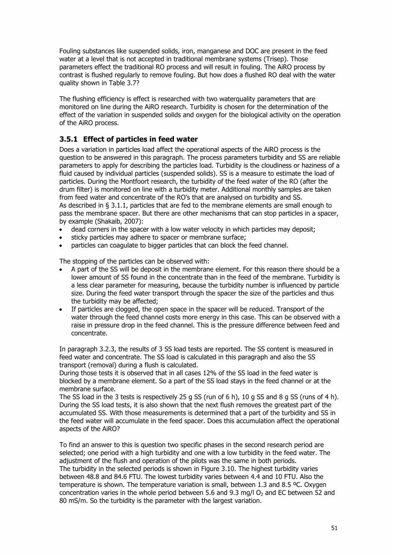
51

Fouling substances like suspended solids, iron, manganese and DOC are present in the feed water at a level that is not accepted in traditional membrane systems (Trisep). Those parameters effect the traditional RO process and will result in fouling. The AiRO process by contrast is flushed regularly to remove fouling. But how does a flushed RO deal with the water quality shown in Table 3.7? The flushing efficiency is effect is researched with two waterquality parameters that are monitored on line during the AiRO research. Turbidity is chosen for the determination of the effect of the variation in suspended solids and oxygen for the biological activity on the operation of the AiRO process.

3.5.1 Effect of particles in feed water

Does a variation in particles load affect the operational aspects of the AiRO process is the question to be answered in this paragraph. The process parameters turbidity and SS are reliable parameters to apply for describing the particles load. Turbidity is the cloudiness or haziness of a fluid caused by individual particles (suspended solids). SS is a measure to estimate the load of particles. During the Montfoort research, the turbidity of the feed water of the RO (after the drum filter) is monitored on line with a turbidity meter. Additional monthly samples are taken from feed water and concentrate of the RO’s that are analysed on turbidity and SS. As described in § 3.1.1, particles that are fed to the membrane elements are small enough to pass the membrane spacer. But there are other mechanisms that can stop particles in a spacer, by example (Shakaib, 2007): dead corners in the spacer with a low water velocity in which particles may deposit; sticky particles may adhere to spacer or membrane surface; particles can coagulate to bigger particles that can block the feed channel. The stopping of the particles can be observed with: A part of the SS will be deposit in the membrane element. For this reason there should be a

lower amount of SS found in the concentrate than in the feed of the membrane. Turbidity is a less clear parameter for measuring, because the turbidity number is influenced by particle size. During the feed water transport through the spacer the size of the particles and thus the turbidity may be affected;

If particles are clogged, the open space in the spacer will be reduced. Transport of the water through the feed channel costs more energy in this case. This can be observed with a raise in pressure drop in the feed channel. This is the pressure difference between feed and concentrate.

In paragraph 3.2.3, the results of 3 SS load tests are reported. The SS content is measured in feed water and concentrate. The SS load is calculated in this paragraph and also the SS transport (removal) during a flush is calculated. During those tests it is observed that in all cases 12% of the SS load in the feed water is blocked by a membrane element. So a part of the SS load stays in the feed channel or at the membrane surface. The SS load in the 3 tests is respectively 25 g SS (run of 6 h), 10 g SS and 8 g SS (runs of 4 h). During the SS load tests, it is also shown that the next flush removes the greatest part of the accumulated SS. With those measurements is determined that a part of the turbidity and SS in the feed water will accumulate in the feed spacer. Does this accumulation affect the operational aspects of the AiRO? To find an answer to this is question two specific phases in the second research period are selected; one period with a high turbidity and one with a low turbidity in the feed water. The adjustment of the flush and operation of the pilots was the same in both periods. The turbidity in the selected periods is shown in Figure 3.10. The highest turbidity varies between 48.8 and 84.6 FTU. The lowest turbidity varies between 4.4 and 10 FTU. Also the temperature is shown. The temperature variation is small, between 1.3 and 8.5 ºC. Oxygen concentration varies in the whole period between 5.6 and 9.3 mg/l O2 and EC between 52 and 80 mS/m. So the turbidity is the parameter with the largest variation.

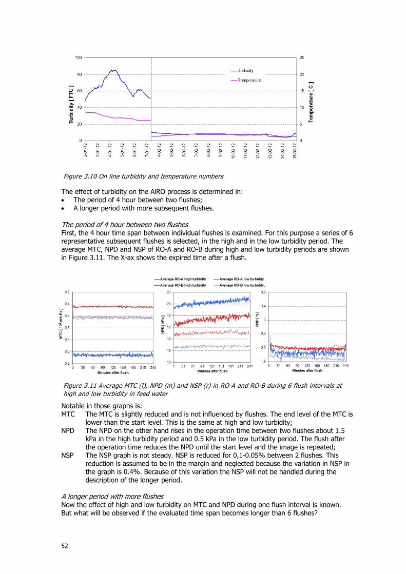
52

The effect of turbidity on the AiRO process is determined in: The period of 4 hour between two flushes; A longer period with more subsequent flushes. The period of 4 hour between two flushes First, the 4 hour time span between individual flushes is examined. For this purpose a series of 6 representative subsequent flushes is selected, in the high and in the low turbidity period. The average MTC, NPD and NSP of RO-A and RO-B during high and low turbidity periods are shown in Figure 3.11. The X-ax shows the expired time after a flush.

Notable in those graphs is: MTC The MTC is slightly reduced and is not influenced by flushes. The end level of the MTC is

lower than the start level. This is the same at high and low turbidity; NPD The NPD on the other hand rises in the operation time between two flushes about 1.5

kPa in the high turbidity period and 0.5 kPa in the low turbidity period. The flush after the operation time reduces the NPD until the start level and the image is repeated;

NSP The NSP graph is not steady. NSP is reduced for 0,1-0.05% between 2 flushes. This reduction is assumed to be in the margin and neglected because the variation in NSP in the graph is 0.4%. Because of this variation the NSP will not be handled during the description of the longer period.

A longer period with more flushes Now the effect of high and low turbidity on MTC and NPD during one flush interval is known. But what will be observed if the evaluated time span becomes longer than 6 flushes?

Figure 3.10 On line turbidity and temperature numbers

Figure 3.11 Average MTC (l), NPD (m) and NSP (r) in RO-A and RO-B during 6 flush intervals at

high and low turbidity in feed water

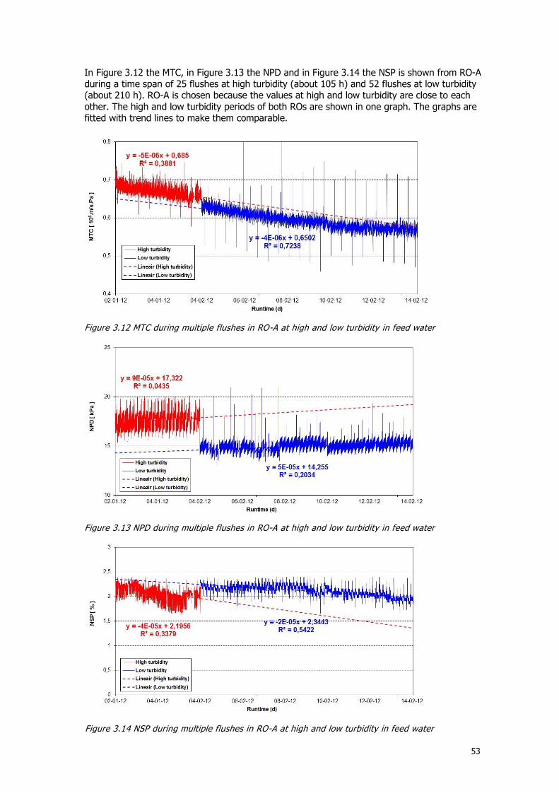
53

In Figure 3.12 the MTC, in Figure 3.13 the NPD and in Figure 3.14 the NSP is shown from RO-A during a time span of 25 flushes at high turbidity (about 105 h) and 52 flushes at low turbidity (about 210 h). RO-A is chosen because the values at high and low turbidity are close to each other. The high and low turbidity periods of both ROs are shown in one graph. The graphs are fitted with trend lines to make them comparable.

Figure 3.12 MTC during multiple flushes in RO-A at high and low turbidity in feed water

Figure 3.13 NPD during multiple flushes in RO-A at high and low turbidity in feed water

Figure 3.14 NSP during multiple flushes in RO-A at high and low turbidity in feed water

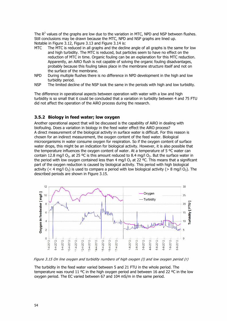
54

The R2 values of the graphs are low due to the variation in MTC, NPD and NSP between flushes. Still conclusions may be drawn because the MTC, NPD and NSP graphs are lined up. Notable in Figure 3.12, Figure 3.13 and Figure 3.14 is: MTC The MTC is reduced in all graphs and the decline angle of all graphs is the same for low

and high turbidity. The MTC is reduced, but particles seem to have no effect on the reduction of MTC in time. Organic fouling can be an explanation for this MTC reduction. Apparently, an AiRO flush is not capable of solving the organic fouling disadvantages, probably because this fouling takes place in the membrane structure itself and not on the surface of the membrane.

NPD During multiple flushes there is no difference in NPD development in the high and low turbidity period.

NSP The limited decline of the NSP look the same in the periods with high and low turbidity. The difference in operational aspects between operation with water with a low and high turbidity is so small that it could be concluded that a variation in turbidity between 4 and 75 FTU did not affect the operation of the AiRO process during the research.

3.5.2 Biology in feed water; low oxygen

Another operational aspect that will be discussed is the capability of AiRO in dealing with biofouling. Does a variation in biology in the feed water effect the AiRO process? A direct measurement of the biological activity in surface water is difficult. For this reason is chosen for an indirect measurement, the oxygen content of the feed water. Biological microorganisms in water consume oxygen for respiration. So if the oxygen content of surface water drops, this might be an indication for biological activity. However, it is also possible that the temperature influences the oxygen content of water. At a temperature of 5 ºC water can contain 12.8 mg/l O2, at 25 ºC is this amount reduced to 8.4 mg/l O2. But the surface water in the period with low oxygen contained less than 4 mg/l O2 at 22 ºC. This means that a significant part of the oxygen reduction is caused by biological activity. This period with high biological activity (< 4 mg/l O2) is used to compare a period with low biological activity (> 8 mg/l O2). The described periods are shown in Figure 3.15.

The turbidity in the feed water varied between 5 and 21 FTU in the whole period. The temperature was round 11 ºC in the high oxygen period and between 16 and 22 ºC in the low oxygen period. The EC varied between 67 and 104 mS/m in the same period.

Figure 3.15 On line oxygen and turbidity numbers of high oxygen (l) and low oxygen period (r)

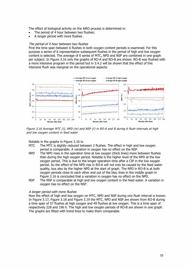
55

The effect of biological activity on the AiRO process is determined in: The period of 4 hour between two flushes; A longer period with more flushes . The period of 4 hour between two flushes First the time span between 6 flushes in both oxygen content periods is examined. For this purpose a series of 6 representative subsequent flushes in the period of high and low oxygen content is selected. The average of 6 series of MTC, NPD and NSP are combined in one graph per subject. In Figure 3.16 only the graphs of RO-A and RO-B are shown. RO-B was flushed with a more intensive program in this period but in 3.4.2 will be shown that the effect of this intensive flush was marginal on the operational aspects.

Notable in the graphs in Figure 3.16 is: MTC The MTC is slightly reduced between 2 flushes. The effect in high and low oxygen

period is comparable. A variation in oxygen has no effect on the NSP. NPD The NPD rises in the operation time at low oxygen (thick lines) more between flushes

than during the high oxygen period. Notable is the higher level of the NPD at the low oxygen period. This is due to the longer operation time after a CIP in the low oxygen period. So the effect of the NPD rise in RO-A will not only be caused by the feed water quality, bus also by the higher NPD at the start of graph. The NPD in RO-B is at both oxygen periods close to each other and out of the bleu lines in the middle graph in Figure 3.16 is concluded that a variation in oxygen has no effect on the NPD.

NSP The NSP is comparable at high and low oxygen content in the feed water. A variation in oxygen has no effect on the NSP.

A longer period with more flushes Now the effect of high and low oxygen on MTC, NPD and NSP during one flush interval is known. In Figure 3.17, Figure 3.18 and Figure 3.19 the MTC, NPD and NSP are shown from RO-B during a time span of 57 flushes at high oxygen and 49 flushes at low oxygen. This is a time span of respectively 228 and 196 h. The high and low oxygen periods of RO-B are shown in one graph. The graphs are fitted with trend lines to make them comparable.

Figure 3.16 Average MTC (l), NPD (m) and NSP (r) in RO-A and B during 6 flush intervals at high

and low oxygen content in feed water

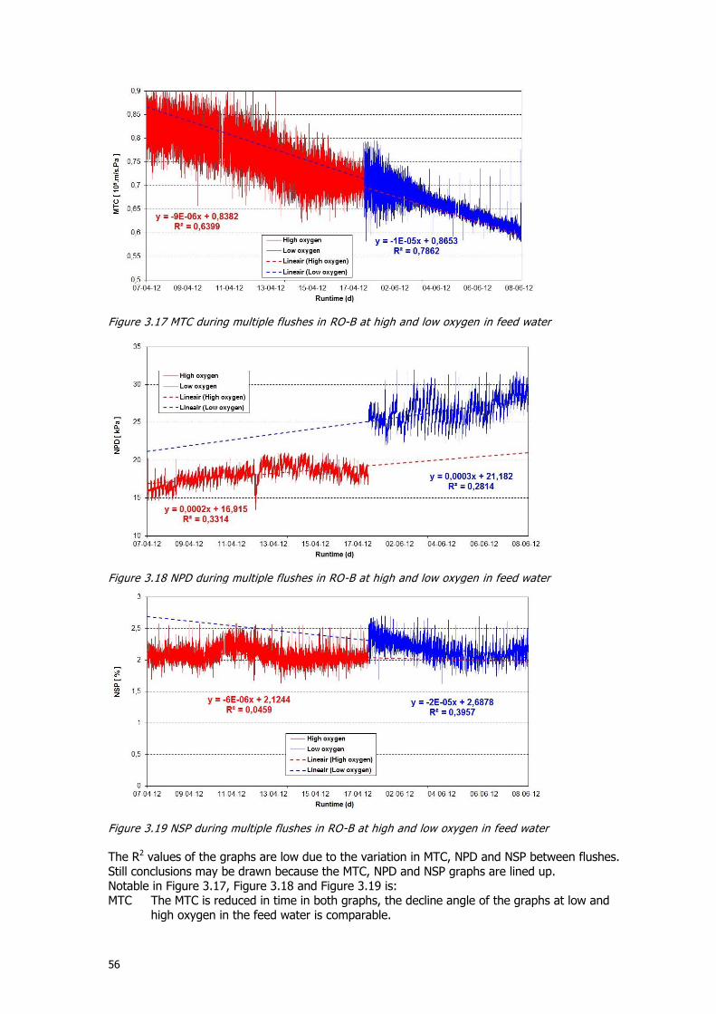
56

Figure 3.17 MTC during multiple flushes in RO-B at high and low oxygen in feed water

Figure 3.19 NSP during multiple flushes in RO-B at high and low oxygen in feed water

The R2 values of the graphs are low due to the variation in MTC, NPD and NSP between flushes. Still conclusions may be drawn because the MTC, NPD and NSP graphs are lined up. Notable in Figure 3.17, Figure 3.18 and Figure 3.19 is: MTC The MTC is reduced in time in both graphs, the decline angle of the graphs at low and

high oxygen in the feed water is comparable.

Figure 3.18 NPD during multiple flushes in RO-B at high and low oxygen in feed water

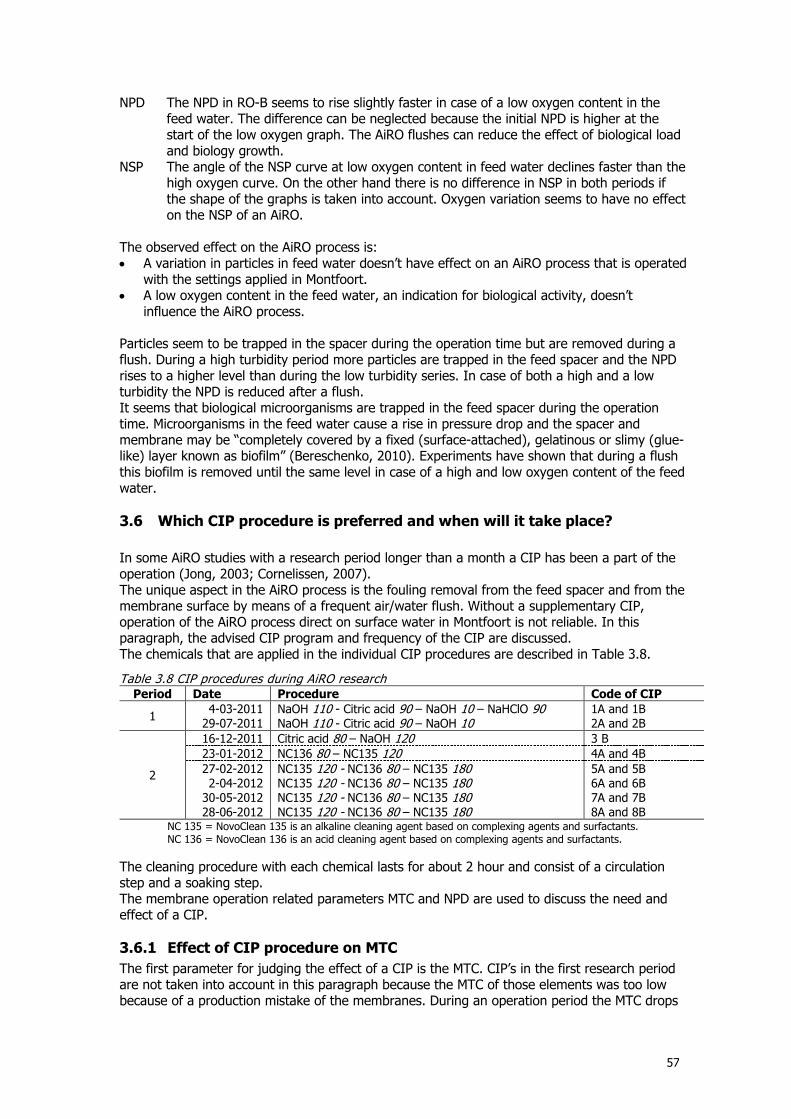
57

NPD The NPD in RO-B seems to rise slightly faster in case of a low oxygen content in the feed water. The difference can be neglected because the initial NPD is higher at the start of the low oxygen graph. The AiRO flushes can reduce the effect of biological load and biology growth.

NSP The angle of the NSP curve at low oxygen content in feed water declines faster than the high oxygen curve. On the other hand there is no difference in NSP in both periods if the shape of the graphs is taken into account. Oxygen variation seems to have no effect on the NSP of an AiRO.

The observed effect on the AiRO process is: A variation in particles in feed water doesn’t have effect on an AiRO process that is operated

with the settings applied in Montfoort. A low oxygen content in the feed water, an indication for biological activity, doesn’t

influence the AiRO process. Particles seem to be trapped in the spacer during the operation time but are removed during a flush. During a high turbidity period more particles are trapped in the feed spacer and the NPD rises to a higher level than during the low turbidity series. In case of both a high and a low turbidity the NPD is reduced after a flush. It seems that biological microorganisms are trapped in the feed spacer during the operation time. Microorganisms in the feed water cause a rise in pressure drop and the spacer and membrane may be “completely covered by a fixed (surface-attached), gelatinous or slimy (glue-like) layer known as biofilm” (Bereschenko, 2010). Experiments have shown that during a flush this biofilm is removed until the same level in case of a high and low oxygen content of the feed water.

3.6 Which CIP procedure is preferred and when will it take place?

In some AiRO studies with a research period longer than a month a CIP has been a part of the operation (Jong, 2003; Cornelissen, 2007). The unique aspect in the AiRO process is the fouling removal from the feed spacer and from the membrane surface by means of a frequent air/water flush. Without a supplementary CIP, operation of the AiRO process direct on surface water in Montfoort is not reliable. In this paragraph, the advised CIP program and frequency of the CIP are discussed. The chemicals that are applied in the individual CIP procedures are described in Table 3.8.

Table 3.8 CIP procedures during AiRO research Period Date Procedure Code of CIP

1 4-03-2011

29-07-2011 NaOH 110 - Citric acid 90 – NaOH 10 – NaHClO 90 NaOH 110 - Citric acid 90 – NaOH 10

1A and 1B 2A and 2B

2

16-12-2011 Citric acid 80 – NaOH 120 3 B

23-01-2012 NC136 80 – NC135 120 4A and 4B

27-02-2012 2-04-2012

30-05-2012 28-06-2012

NC135 120 - NC136 80 – NC135 180 NC135 120 - NC136 80 – NC135 180 NC135 120 - NC136 80 – NC135 180 NC135 120 - NC136 80 – NC135 180

5A and 5B 6A and 6B 7A and 7B 8A and 8B

NC 135 = NovoClean 135 is an alkaline cleaning agent based on complexing agents and surfactants. NC 136 = NovoClean 136 is an acid cleaning agent based on complexing agents and surfactants.

The cleaning procedure with each chemical lasts for about 2 hour and consist of a circulation step and a soaking step. The membrane operation related parameters MTC and NPD are used to discuss the need and effect of a CIP.

3.6.1 Effect of CIP procedure on MTC

The first parameter for judging the effect of a CIP is the MTC. CIP’s in the first research period are not taken into account in this paragraph because the MTC of those elements was too low because of a production mistake of the membranes. During an operation period the MTC drops

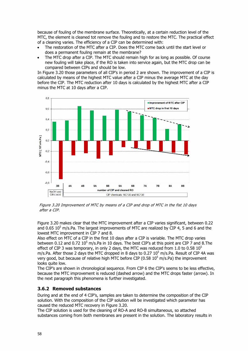
58

because of fouling of the membrane surface. Theoretically, at a certain reduction level of the MTC, the element is cleaned tot remove the fouling and to restore the MTC. The practical effect of a cleaning varies. The efficiency of a CIP can be determined with: The restoration of the MTC after a CIP. Does the MTC come back until the start level or

does a permanent fouling remain at the membrane? The MTC drop after a CIP. The MTC should remain high for as long as possible. Of course

new fouling will take place, if the RO is taken into service again, but the MTC drop can be compared between CIPs and should be low.

In Figure 3.20 those parameters of all CIP’s in period 2 are shown. The improvement of a CIP is calculated by means of the highest MTC value after a CIP minus the average MTC at the day before the CIP. The MTC reduction after 10 days is calculated by the highest MTC after a CIP minus the MTC at 10 days after a CIP.

Figure 3.20 makes clear that the MTC improvement after a CIP varies significant, between 0.22 and 0.65 105 m/s.Pa. The largest improvements of MTC are realized by CIP 4, 5 and 6 and the lowest MTC improvement in CIP 7 and 8. Also effect on MTC of a CIP in the first 10 days after a CIP is variable. The MTC drop varies between 0.12 and 0.72 105 m/s.Pa in 10 days. The best CIP’s at this point are CIP 7 and 8.The effect of CIP 3 was temporary, in only 2 days, the MTC was reduced from 1.0 to 0.58 105 m/s.Pa. After those 2 days the MTC dropped in 8 days to 0.27 105 m/s.Pa. Result of CIP 4A was very good, but because of relative high MTC before CIP (0.58 105 m/s.Pa) the improvement looks quite low. The CIP’s are shown in chronological sequence. From CIP 6 the CIP’s seems to be less effective, because the MTC improvement is reduced (dashed arrow) and the MTC drops faster (arrow). In the next paragraph this phenomena is further investigated.

3.6.2 Removed substances

During and at the end of 4 CIP’s, samples are taken to determine the composition of the CIP solution. With the composition of the CIP solution will be investigated which parameter has caused the reduced MTC recovery in Figure 3.20. The CIP solution is used for the cleaning of RO-A and RO-B simultaneous, so attached substances coming from both membranes are present in the solution. The laboratory results in

Figure 3.20 Improvement of MTC by means of a CIP and drop of MTC in the fist 10 days

after a CIP.

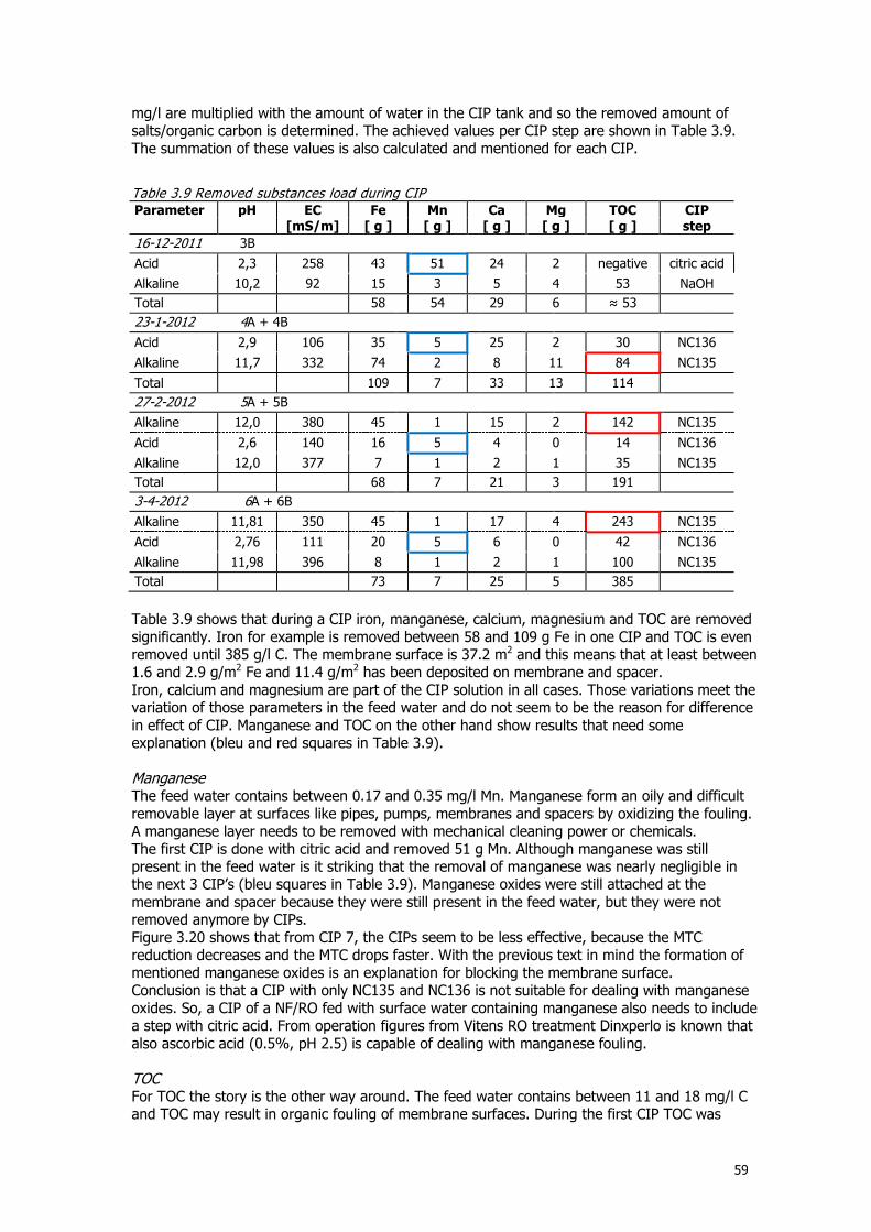
59

mg/l are multiplied with the amount of water in the CIP tank and so the removed amount of salts/organic carbon is determined. The achieved values per CIP step are shown in Table 3.9. The summation of these values is also calculated and mentioned for each CIP.

Table 3.9 Removed substances load during CIP

Parameter pH EC Fe Mn Ca Mg TOC CIP [mS/m] [ g ] [ g ] [ g ] [ g ] [ g ] step

16-12-2011 3B

Acid 2,3 258 43 51 24 2 negative citric acid

Alkaline 10,2 92 15 3 5 4 53 NaOH

Total 58 54 29 6 ≈ 53

23-1-2012 4A + 4B

Acid 2,9 106 35 5 25 2 30 NC136

Alkaline 11,7 332 74 2 8 11 84 NC135

Total 109 7 33 13 114

27-2-2012 5A + 5B

Alkaline 12,0 380 45 1 15 2 142 NC135

Acid 2,6 140 16 5 4 0 14 NC136

Alkaline 12,0 377 7 1 2 1 35 NC135

Total 68 7 21 3 191

3-4-2012 6A + 6B

Alkaline 11,81 350 45 1 17 4 243 NC135

Acid 2,76 111 20 5 6 0 42 NC136

Alkaline 11,98 396 8 1 2 1 100 NC135

Total 73 7 25 5 385

Table 3.9 shows that during a CIP iron, manganese, calcium, magnesium and TOC are removed significantly. Iron for example is removed between 58 and 109 g Fe in one CIP and TOC is even removed until 385 g/l C. The membrane surface is 37.2 m2 and this means that at least between 1.6 and 2.9 g/m2 Fe and 11.4 g/m2 has been deposited on membrane and spacer. Iron, calcium and magnesium are part of the CIP solution in all cases. Those variations meet the variation of those parameters in the feed water and do not seem to be the reason for difference in effect of CIP. Manganese and TOC on the other hand show results that need some explanation (bleu and red squares in Table 3.9). Manganese The feed water contains between 0.17 and 0.35 mg/l Mn. Manganese form an oily and difficult removable layer at surfaces like pipes, pumps, membranes and spacers by oxidizing the fouling. A manganese layer needs to be removed with mechanical cleaning power or chemicals. The first CIP is done with citric acid and removed 51 g Mn. Although manganese was still present in the feed water is it striking that the removal of manganese was nearly negligible in the next 3 CIP’s (bleu squares in Table 3.9). Manganese oxides were still attached at the membrane and spacer because they were still present in the feed water, but they were not removed anymore by CIPs. Figure 3.20 shows that from CIP 7, the CIPs seem to be less effective, because the MTC reduction decreases and the MTC drops faster. With the previous text in mind the formation of mentioned manganese oxides is an explanation for blocking the membrane surface. Conclusion is that a CIP with only NC135 and NC136 is not suitable for dealing with manganese oxides. So, a CIP of a NF/RO fed with surface water containing manganese also needs to include a step with citric acid. From operation figures from Vitens RO treatment Dinxperlo is known that also ascorbic acid (0.5%, pH 2.5) is capable of dealing with manganese fouling. TOC For TOC the story is the other way around. The feed water contains between 11 and 18 mg/l C and TOC may result in organic fouling of membrane surfaces. During the first CIP TOC was

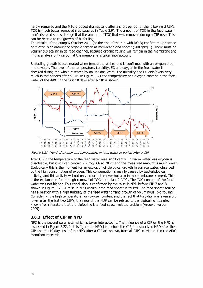
60

hardly removed and the MTC dropped dramatically after a short period. In the following 3 CIP’s TOC is much better removed (red squares in Table 3.9). The amount of TOC in the feed water didn’t rise and so it’s strange that the amount of TOC that was removed during a CIP rose. This can be related to the growth of biofouling. The results of the autopsy October 2011 (at the end of the run with RO-B) confirm the presence of relative high amount of organic carbon at membrane and spacer (200 g/kg C). There must be voluminous scaling in de feed channel, because organic fouling will remain in the membrane and in this analysis only carbon at the membrane is taken into account. Biofouling growth is accelerated when temperature rises and is confirmed with an oxygen drop in the water. The level of the temperature, turbidity, EC and oxygen in the feed water is checked during the whole research by on line analyzers. The turbidity and EC didn’t vary very much in the periods after a CIP. In Figure 3.21 the temperature and oxygen content in the feed water of the AiRO in the first 10 days after a CIP is shown.

After CIP 7 the temperature of the feed water rose significantly. In warm water less oxygen is dissolvable, but it still can contain 9.2 mg/l O2 at 20 ºC and the measured amount is much lower. Ecologically this is the moment for an explosion of biological growth in surface water, observed by the high consumption of oxygen. This consumption is mainly caused by bacteriological activity, and this activity will not only occur in the river but also in the membrane element. This is the explanation for the high removal of TOC in the last 2 CIP’s. The TOC content of the feed water was not higher. This conclusion is confirmed by the raise in NPD before CIP 7 and 8, shown in Figure 3.20. A raise in NPD occurs if the feed spacer is fouled. The feed spacer fouling has a relation with a high turbidity of the feed water or/and growth of voluminous (bio)fouling. Considering the high temperature, low oxygen content and the fact that turbidity was even a bit lower after the last two CIP’s, the raise of the NDP can be related to the biofouling. It’s also known from literature that the biofouling is a feed spacer related problem (Vrouwenvelder, 2009).

3.6.3 Effect of CIP on NPD

NPD is the second parameter which is taken into account. The influence of a CIP on the NPD is discussed in Figure 3.22. In this figure the NPD just before the CIP, the stabilized NPD after the CIP and the 10 days rise of the NPD after a CIP are shown, from all CIP’s carried out in the AiRO Montfoort research.

Figure 3.21 Trend of oxygen and temperature in feed water in period after a CIP

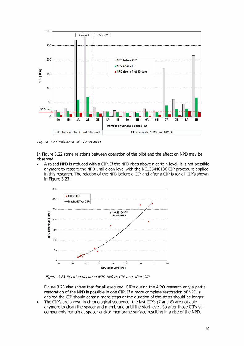
61

In Figure 3.22 some relations between operation of the pilot and the effect on NPD may be observed: A raised NPD is reduced with a CIP. If the NPD rises above a certain level, it is not possible

anymore to restore the NPD until clean level with the NC135/NC136 CIP procedure applied in this research. The relation of the NPD before a CIP and after a CIP is for all CIP’s shown in Figure 3.23.

Figure 3.23 also shows that for all executed CIP’s during the AiRO research only a partial restoration of the NPD is possible in one CIP. If a more complete restoration of NPD is desired the CIP should contain more steps or the duration of the steps should be longer.

The CIP’s are shown in chronological sequence; the last CIP’s (7 and 8) are not able anymore to clean the spacer and membrane until the start level. So after those CIPs still components remain at spacer and/or membrane surface resulting in a rise of the NPD.

Figure 3.22 Influence of CIP on NPD

Figure 3.23 Relation between NPD before CIP and after CIP

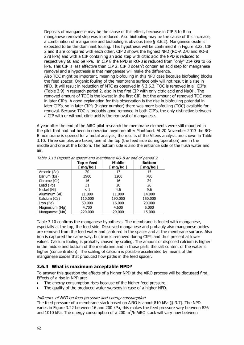
62

Deposits of manganese may be the cause of this effect, because in CIP 5 to 8 no manganese removal step was introduced. Also biofouling may be the cause of this increase, a combination of manganese and biofouling is obvious (see § 3.6.2). Manganese oxide is expected to be the dominant fouling. This hypothesis will be confirmed if in Figure 3.22. CIP 2 and 8 are compared with each other. CIP 2 shows the highest NPD (RO-A 270 and RO-B 278 kPa) and with a CIP containing an acid step with citric acid the NPD is reduced to respectively 60 and 69 kPa. In CIP 8 the NPD in RO-B is reduced from “only“ 214 kPa to 66 kPa. This CIP is less effective than CIP 2. CIP 8 doesn’t contain an acid step for manganese removal and a hypothesis is that manganese will make the difference. Also TOC might be important, meaning biofouling in this NPD case because biofouling blocks the feed spacer. Organic fouling of the membrane surface only will not result in a rise in NPD. It will result in reduction of MTC as observed in § 3.6.3. TOC is removed in all CIP’s (Table 3.9) in research period 2, also in the first CIP with only citric acid and NaOH. The removed amount of TOC is the lowest in the first CIP, but the amount of removed TOC rose in later CIP’s. A good explanation for this observation is the rise in biofouling potential in later CIP’s, so in later CIP’s (higher number) there was more biofouling (TOC) available for removal. Because TOC is probably good removed in both CIP’s, the only distinctive between a CIP with or without citric acid is the removal of manganese.

A year after the end of the AiRO pilot research the membrane elements were still mounted in the pilot that had not been in operation anymore after Montfoort. At 20 November 2013 the RO-B membrane is opened for a metal analysis, the results of the Vitens analysis are shown in Table 3.10. Three samples are taken, one at the top (the feed side during operation) one in the middle and one at the bottom. The bottom side is also the entrance side of the flush water and air.

Table 3.10 Deposit at spacer and membrane RO-B at end of period 2 Top = feed

[ mg/kg ] Middle

[ mg/kg ] Bottom

[ mg/kg ]

Arsenic (As) Barium (Ba) Chrome (Cr) Lead (Pb) Nickel (Ni) Aluminum (Al) Calcium (Ca) Iron (Fe) Magnesium (Mg) Manganese (Mn)

20 3900 16 31 < 1

11,000 110,000 50,000 4,700

220,000

13 1200 16 20 4.6

11,000 190,000 16,000 4,600 29,000

15 780 24 26 9.6

14,000 150,000 20,000 5,000 15,000

Table 3.10 confirms the manganese hypothesis. The membrane is fouled with manganese, especially at the top, the feed side. Dissolved manganese and probably also manganese oxides are removed from the feed water and captured in the spacer and at the membrane surface. Also iron is captured the same way, but iron is removed during CIP’s and thus present at lower values. Calcium fouling is probably caused by scaling. The amount of disposed calcium is higher in the middle and bottom of the membrane and in those parts the salt content of the water is higher (concentration). The scaling of calcium is possible accelerated by means of the manganese oxides that produced flow paths in the feed spacer.

3.6.4 What is maximum acceptable NPD?

To answer this question the effects of a higher NPD at the AiRO process will be discussed first. Effects of a rise in NPD are: The energy consumption rises because of the higher feed pressure; The quality of the produced water worsens in case of a higher NPD. Influence of NPD on feed pressure and energy consumption The feed pressure of a membrane stack based on AiRO is about 810 kPa (§ 3.7). The NPD varies in Figure 3.22 between 16 and 200 kPa, this makes the feed pressure vary between 826 and 1010 kPa. The energy consumption of a 200 m3/h AiRO stack will vary now between

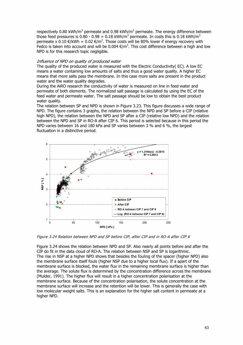
63

respectively 0.80 kWh/m3 permeate and 0.98 kWh/m3 permeate. The energy difference between those feed pressures is 0.80 - 0.98 = 0.18 kWh/m3 permeate. In costs this is 0.18 kWh/m3 permeate x 0.10 €/kWh = 0.02 €/m3. Those costs will be 80% lower if energy recovery with Fedco is taken into account and will be 0.004 €/m3. This cost difference between a high and low NPD is for this research topic negligible. Influence of NPD on quality of produced water The quality of the produced water is measured with the Electric Conductivity( EC). A low EC means a water containing low amounts of salts and thus a good water quality. A higher EC means that more salts pass the membrane. In this case more salts are present in the product water and the water quality degrades. During the AiRO research the conductivity of water is measured on line in feed water and permeate of both elements. The normalized salt passage is calculated by using the EC of the feed water and permeate water. The salt passage should be low to obtain the best product water quality. The relation between SP and NPD is shown in Figure 3.23. This figure discusses a wide range of NPD. The figure contains 3 graphs, the relation between the NPD and SP before a CIP (relative high NPD), the relation between the NPD and SP after a CIP (relative low NPD) and the relation between the NPD and SP in RO-A after CIP 6. This period is selected because in this period the NPD varies between 16 and 180 kPa and SP varies between 3 % and 6 %, the largest fluctuation in a distinctive period.

Figure 3.24 Relation between NPD and SP before CIP, after CIP and in RO-A after CIP 6

Figure 3.24 shows the relation between NPD and SP. Also nearly all points before and after the CIP do fit in the data cloud of RO-A. The relation between NSP and SP is logarithmic. The rise in NSP at a higher NPD shows that besides the fouling of the spacer (higher NPD) also the membrane surface itself fouls (higher NSP due to a higher local flux). If a apart of the membrane surface is blocked, the water flux in the remaining membrane surface is higher than the average. The solute flux is determined by the concentration difference across the membrane (Mulder, 1991). The higher flux will result in a higher concentration polarisation at the membrane surface. Because of the concentration polarisation, the solute concentration at the membrane surface will increase and the retention will be lower. This is generally the case with low molecular weight salts. This is an explanation for the higher salt content in permeate at a higher NPD.

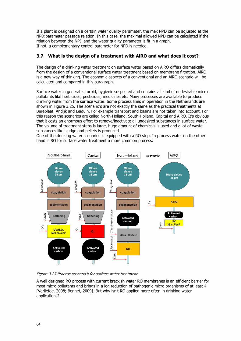
64

If a plant is designed on a certain water quality parameter, the max NPD can be adjusted at the NPD:parameter passage relation. In this case, the maximal allowed NPD can be calculated if the relation between the NPD and the water quality parameter is fit in a graph. If not, a complementary control parameter for NPD is needed.

3.7 What is the design of a treatment with AiRO and what does it cost?

The design of a drinking water treatment on surface water based on AiRO differs dramatically from the design of a conventional surface water treatment based on membrane filtration. AiRO is a new way of thinking. The economic aspects of a conventional and an AiRO scenario will be calculated and compared in this paragraph. Surface water in general is turbid, hygienic suspected and contains all kind of undesirable micro pollutants like herbicides, pesticides, medicines etc. Many processes are available to produce drinking water from the surface water. Some process lines in operation in the Netherlands are shown in Figure 3.25. The scenario’s are not exactly the same as the practical treatments at Bereplaat, Andijk and Leiduin. For example transport and basins are not taken into account. For this reason the scenarios are called North-Holland, South-Holland, Capital and AiRO. It’s obvious that it costs an enormous effort to remove/inactivate all undesired substances in surface water. The volume of treatment steps is large, huge amount of chemicals is used and a lot of waste substances like sludge and pellets is produced. One of the drinking water scenarios is equipped with a RO step. In process water on the other hand is RO for surface water treatment a more common process.

A well designed RO process with current brackish water RO membranes is an efficient barrier for most micro pollutants and brings in a log reduction of pathogenic micro organisms of at least 4 [Verliefde, 2008; Bennet, 2009]. But why isn’t RO applied more often in drinking water applications?

Figure 3.25 Process scenario’s for surface water treatment

65

Main reasons for this draw back are: An extensive pretreatment is necessary to prevent (bio)fouling in the RO; Even with an extensive pretreatment the RO has to be cleaned regular; Disposal of the concentrate is a challenge; In previous paragraphs is mentioned that AiRO is able to produce RO permeate with an extensive pretreatment but how will AiRO deal with the draw backs of the extended process scheme North-Holland in Figure 3.25? (Bio)fouling in the RO is prevented with a 4 minute air water flush every 4 hours. Only

compressed air and feed water are required for this cleaning; A CIP of the AiRO takes place every month and that is less frequent than in many traditional

RO’s; The disposal of the concentrate is also a challenge for AiRO, but in this case the low

recovery and the absence of antiscalant is an advantage of AiRO. This results in a less concentrated water quality, compared to traditional RO at 80%-85% recovery. The concentrate should be disposed down flow of the intake point of the feed water.

The lay out of a possible process scheme with AiRO is also shown in Figure 3.25. Purpose of the steps mentioned in the scheme are: Micro sieves Rotating micro sieves to remove particulate fouling above 35 µm. This mesh

size is much smaller than the 120 µm applied during the research, but is chosen because of the good results obtained in The Netherlands with this robust water treatment technology;

AiRO Removal of salts, pathogens, organic compounds and micro pollutants from the water. The permeate will be de-acidified in a CO2 strip tower.;

Activated carbon Removal of the last small non polar substances from the water. Contact time is short, 5 minutes only;

UV disinfection Taking care of a microbial log removal of 8 in total with a UV dose of 35 mJ/cm;

Blending Dosing calcium until the desired level of 1 mmol/l lime content. Blending with calcium rich groundwater should be the most elegant solution.

3.7.1 What will an AiRO stack design look like?

A stack design starts with the determination of a representative feed water quality. In this case Hollandse IJssel water will be applied (Table 3.11). This table contains the max values of the parameters and of an extreme feed water quality determined at 12 April 2012. These values are applied in the projection calculations.

Table 3.11 Water quality applied in projection calculations Parameter Analysis used for

projection 12-04-2012

Max in feed of pilot Analysis Vitens lab.

pH value Temperature [°C]

8 10.7

6.9 < pH < 8.2 2.3 < T < 20.3

Calcium [mg/l Ca] Magnesium [mg/l Mg] Sodium [mg/l Na] Potassium [mg/l K] Barium [µg/l Ba] Strontium [µg/l Sr]

92 13 63 8.8 70 490

92.0 13.3 63.0 10.2 71.6 494

Sulfate [mg/l SO4] Nitrate [mg/l NO3] Chloride [mg/l Cl] Bicarbonate [mg/l HCO3]

74 7

101 246

119.6 11.0 101.3 246.2

The comparison between a traditional design and a AiRO design will be made by means of a stack with a capacity of 200 m3/h permeate.

66

The applied membrane will be the same as during the pilot research. The average design flux is higher than during the experiments. The design of a traditional RO stack and two AiRO configurations are calculated with TROI [TriSep, version 2.5.0] and are summarized in Table 3.12.

Table 3.12 Design of a traditional stack and of an AiRO stack

Parameter Traditional

design AiRO design

1 element vessel AiRO design

2 element vessel

Membrane [Trisep] Average flux [l/m2/h] Permeate [m3/h]

8040-ACM5-UWA 23 200

8040-ACM5-UWA 26 200

8040-ACM5-UWA 26 200

Recovery [%] Feed [m3/h] Feed pressure [kPa] Concentrate pressure [kPa] Antiscalant [yes/no] Acid [yes/no]

80 250 880 730 yes no

35 571 790 790 no no

35 571 810 780 no no

Stages [n] Elements per vessel [n] Vessels [n] Elements [n in total]

2 6

26 + 13 = 39 156 + 78 = 234

1 1

208 208

1 2

104 208

Flux [lmh] LSI concentrate Beta

25.4 / 18.3 = 23.0 2.48

1.19 / 1.13

25.9 1.00 1.46

25.9 1.00 1.23

The traditional design consists of a 2:1 staging with 26 vessels in the first stage and 13 in the second stage. A feed pressure of 880 kPa is applied and the pressure drop over the stack is 150 kPa. The recovery is about 80% and LSI in the concentrate is 2.48. An antiscalant has to be applied to prevent the scaling on membranes and concentrate piping. The flux in the AiRO elements is in correspondence with the flux in the first elements of stage 1 of the traditional stack. Because of this assumption the ratio of pressure vessels is not the expected 6 but smaller. The traditional design is compared with 2 AiRO designs that will be outlined in next paragraph.

3.7.2 Introduction of 2 element pressure vessel

The original AiRO design is based on 1 element pressure vessels. Also the research in Montfoort is carried out with 2 units of with one element pressure vessels. Point of concern in a stack design based on this pressure vessel is the high amount of short vessels and of pipe connections. The amount of vessels is nearly 5.3 times higher than a traditional stack (39 to 208). The application of a pressure vessel containing 2 elements in series in stead of 1 is a theoretic innovation in this AiRO thesis. This vessel is not tested in practice yet, it’s a theoretic design shown in Figure 3.26. The operation of the new vessel will remain down flow. So the upper element will intercept a part of the stopped particulate fouling. In theory the second element will remain less polluted than the first. In the flush mode, two options are possible; a flush of both elements separated and a flush of both elements at the same time. Committing a separated up flow flush mode of element I and II shown in the middle of Figure 3.26 comes very close to the operation during the pilot research in Montfoort. This method of operating and flushing of a 2 element pressure vessel will be possible without doubt. In the other option, in which the operation still down flow is, the upflow flush mode flushes both elements at the same time. The flush water and air is introduced at the bottom of the pressure vessel and redistributed between both elements with an air-water distribution plate. The pressure drop over the plate will be about 25 kPa during water flush and air is distributed with the same amount of small pipes as there are holes in the air-distribution end connector.

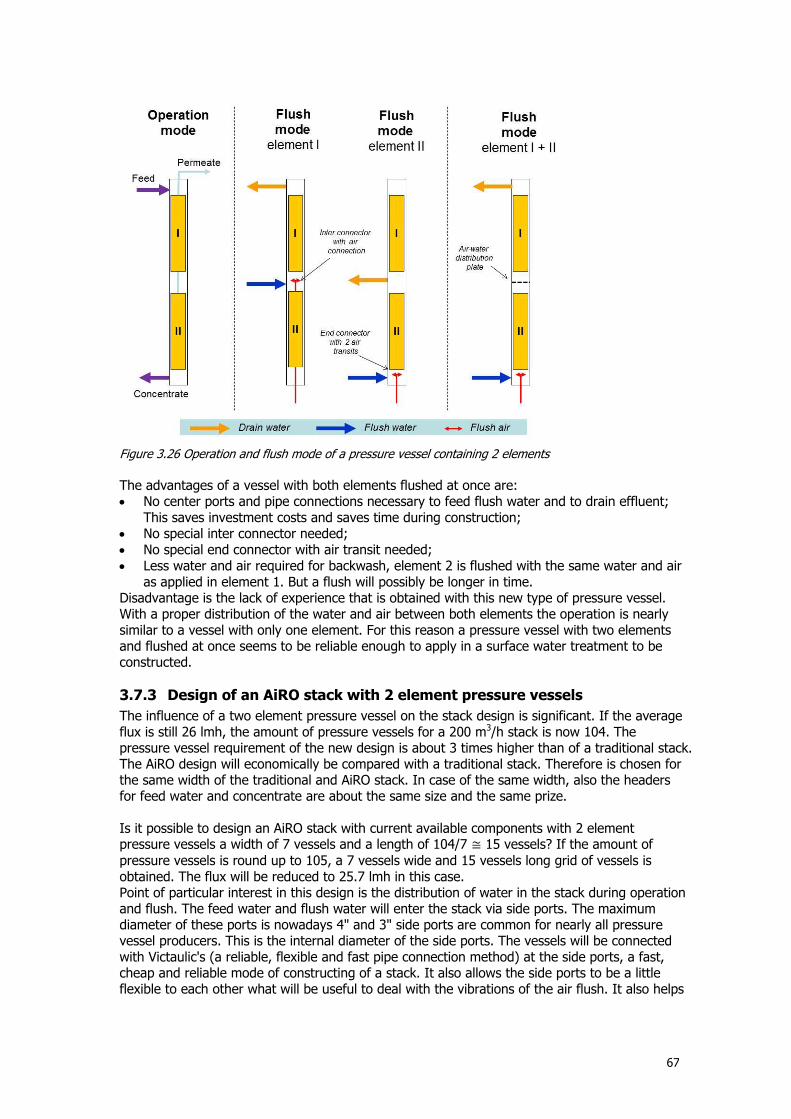
67

Figure 3.26 Operation and flush mode of a pressure vessel containing 2 elements

The advantages of a vessel with both elements flushed at once are: No center ports and pipe connections necessary to feed flush water and to drain effluent;

This saves investment costs and saves time during construction; No special inter connector needed; No special end connector with air transit needed; Less water and air required for backwash, element 2 is flushed with the same water and air

as applied in element 1. But a flush will possibly be longer in time. Disadvantage is the lack of experience that is obtained with this new type of pressure vessel. With a proper distribution of the water and air between both elements the operation is nearly similar to a vessel with only one element. For this reason a pressure vessel with two elements and flushed at once seems to be reliable enough to apply in a surface water treatment to be constructed.

3.7.3 Design of an AiRO stack with 2 element pressure vessels

The influence of a two element pressure vessel on the stack design is significant. If the average flux is still 26 lmh, the amount of pressure vessels for a 200 m3/h stack is now 104. The pressure vessel requirement of the new design is about 3 times higher than of a traditional stack. The AiRO design will economically be compared with a traditional stack. Therefore is chosen for the same width of the traditional and AiRO stack. In case of the same width, also the headers for feed water and concentrate are about the same size and the same prize. Is it possible to design an AiRO stack with current available components with 2 element pressure vessels a width of 7 vessels and a length of 104/7 15 vessels? If the amount of

pressure vessels is round up to 105, a 7 vessels wide and 15 vessels long grid of vessels is obtained. The flux will be reduced to 25.7 lmh in this case. Point of particular interest in this design is the distribution of water in the stack during operation and flush. The feed water and flush water will enter the stack via side ports. The maximum diameter of these ports is nowadays 4" and 3" side ports are common for nearly all pressure vessel producers. This is the internal diameter of the side ports. The vessels will be connected with Victaulic's (a reliable, flexible and fast pipe connection method) at the side ports, a fast, cheap and reliable mode of constructing of a stack. It also allows the side ports to be a little flexible to each other what will be useful to deal with the vibrations of the air flush. It also helps

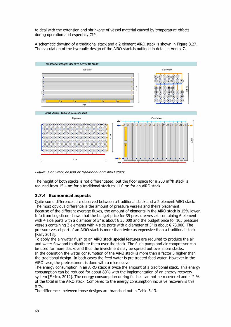
68

to deal with the extension and shrinkage of vessel material caused by temperature effects during operation and especially CIP. A schematic drawing of a traditional stack and a 2 element AiRO stack is shown in Figure 3.27. The calculation of the hydraulic design of the AiRO stack is outlined in detail in Annex 7.

Figure 3.27 Stack design of traditional and AiRO stack

The height of both stacks is not differentiated, but the floor space for a 200 m3/h stack is reduced from 15.4 m2 for a traditional stack to 11.0 m2 for an AiRO stack.

3.7.4 Economical aspects

Quite some differences are observed between a traditional stack and a 2 element AiRO stack. The most obvious difference is the amount of pressure vessels and theirs placement. Because of the different average fluxes, the amount of elements in the AiRO stack is 15% lower. Info from Logisticon shows that the budget price for 39 pressure vessels containing 6 element with 4 side ports with a diameter of 3” is about € 35.000 and the budget price for 105 pressure vessels containing 2 elements with 4 side ports with a diameter of 3” is about € 73.000. The pressure vessel part of an AiRO stack is more than twice as expensive than a traditional stack [Kalf, 2013]. To apply the air/water flush to an AiRO stack special features are required to produce the air and water flow and to distribute them over the stack. The flush pump and air compressor can be used for more stacks and thus the investment may be spread out over more stacks. In the operation the water consumption of the AiRO stack is more than a factor 3 higher than the traditional design. In both cases the feed water is pre treated feed water. However in the AiRO case, the pretreatment is done with a micro sieve. The energy consumption in an AiRO stack is twice the amount of a traditional stack. This energy consumption can be reduced for about 80% with the implementation of an energy recovery system [Fedco, 2012]. The energy consumption during flushes can not be recovered and is 2 % of the total in the AiRO stack. Compared to the energy consumption inclusive recovery is this 8 %. The differences between those designs are branched out in Table 3.13.

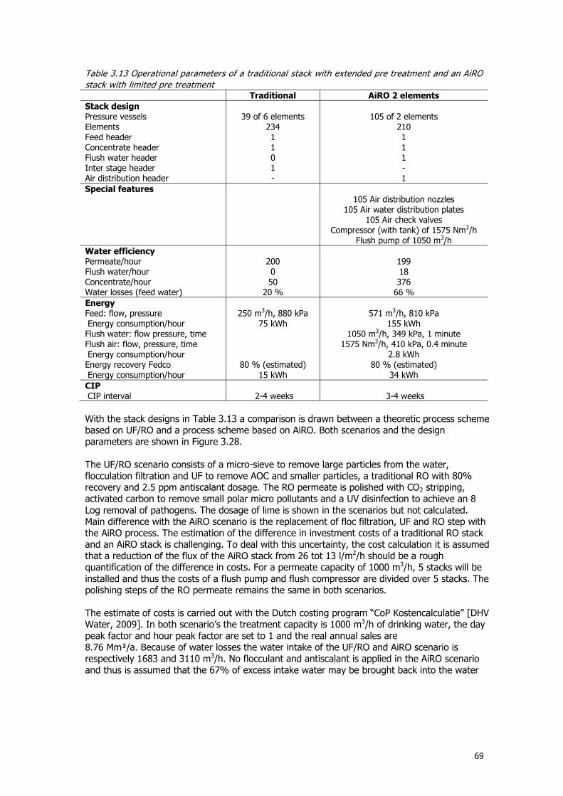
69

Table 3.13 Operational parameters of a traditional stack with extended pre treatment and an AiRO

stack with limited pre treatment Traditional AiRO 2 elements

Stack design Pressure vessels Elements Feed header Concentrate header Flush water header Inter stage header Air distribution header

39 of 6 elements

234 1 1 0 1 -

105 of 2 elements

210 1 1 1 - 1

Special features

105 Air distribution nozzles

105 Air water distribution plates 105 Air check valves

Compressor (with tank) of 1575 Nm3/h Flush pump of 1050 m3/h

Water efficiency Permeate/hour Flush water/hour Concentrate/hour Water losses (feed water)

200 0 50

20 %

199 18 376

66 %

Energy Feed: flow, pressure Energy consumption/hour Flush water: flow pressure, time Flush air: flow, pressure, time Energy consumption/hour Energy recovery Fedco Energy consumption/hour

250 m3/h, 880 kPa

75 kWh

80 % (estimated) 15 kWh

571 m3/h, 810 kPa

155 kWh 1050 m3/h, 349 kPa, 1 minute

1575 Nm3/h, 410 kPa, 0.4 minute 2.8 kWh

80 % (estimated) 34 kWh

CIP CIP interval

2-4 weeks

3-4 weeks

With the stack designs in Table 3.13 a comparison is drawn between a theoretic process scheme based on UF/RO and a process scheme based on AiRO. Both scenarios and the design parameters are shown in Figure 3.28. The UF/RO scenario consists of a micro-sieve to remove large particles from the water, flocculation filtration and UF to remove AOC and smaller particles, a traditional RO with 80% recovery and 2.5 ppm antiscalant dosage. The RO permeate is polished with CO2 stripping, activated carbon to remove small polar micro pollutants and a UV disinfection to achieve an 8 Log removal of pathogens. The dosage of lime is shown in the scenarios but not calculated. Main difference with the AiRO scenario is the replacement of floc filtration, UF and RO step with the AiRO process. The estimation of the difference in investment costs of a traditional RO stack and an AiRO stack is challenging. To deal with this uncertainty, the cost calculation it is assumed that a reduction of the flux of the AiRO stack from 26 tot 13 l/m2/h should be a rough quantification of the difference in costs. For a permeate capacity of 1000 m3/h, 5 stacks will be installed and thus the costs of a flush pump and flush compressor are divided over 5 stacks. The polishing steps of the RO permeate remains the same in both scenarios. The estimate of costs is carried out with the Dutch costing program “CoP Kostencalculatie” [DHV Water, 2009]. In both scenario’s the treatment capacity is 1000 m3/h of drinking water, the day peak factor and hour peak factor are set to 1 and the real annual sales are 8.76 Mm³/a. Because of water losses the water intake of the UF/RO and AiRO scenario is respectively 1683 and 3110 m3/h. No flocculant and antiscalant is applied in the AiRO scenario and thus is assumed that the 67% of excess intake water may be brought back into the water

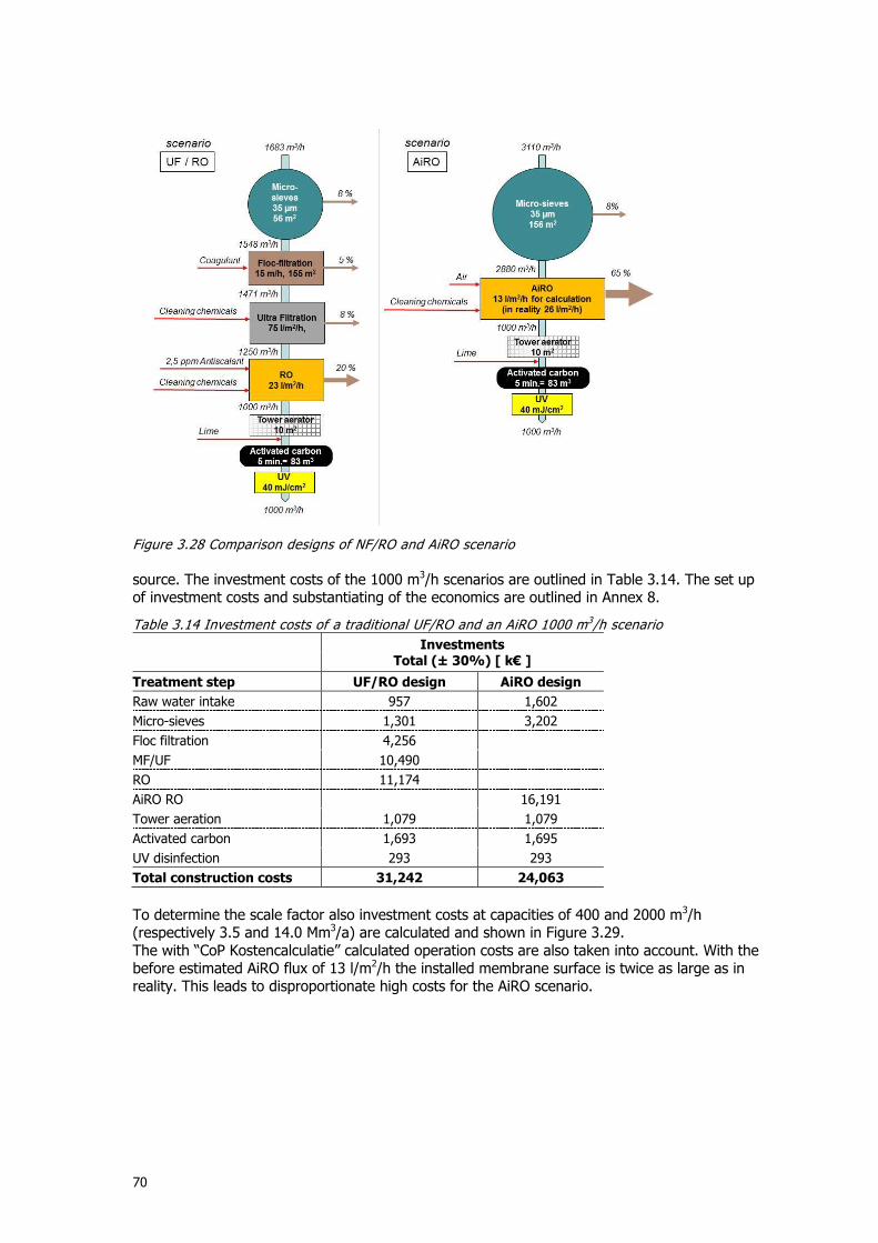
70

Figure 3.28 Comparison designs of NF/RO and AiRO scenario

source. The investment costs of the 1000 m3/h scenarios are outlined in Table 3.14. The set up of investment costs and substantiating of the economics are outlined in Annex 8.

Table 3.14 Investment costs of a traditional UF/RO and an AiRO 1000 m3/h scenario

Investments

Total (± 30%) [ k€ ]

Treatment step UF/RO design AiRO design

Raw water intake 957 1,602

Micro-sieves 1,301 3,202

Floc filtration 4,256

MF/UF 10,490

RO 11,174

AiRO RO

16,191

Tower aeration 1,079 1,079

Activated carbon 1,693 1,695

UV disinfection 293 293

Total construction costs 31,242 24,063

To determine the scale factor also investment costs at capacities of 400 and 2000 m3/h (respectively 3.5 and 14.0 Mm3/a) are calculated and shown in Figure 3.29. The with “CoP Kostencalculatie” calculated operation costs are also taken into account. With the before estimated AiRO flux of 13 l/m2/h the installed membrane surface is twice as large as in reality. This leads to disproportionate high costs for the AiRO scenario.

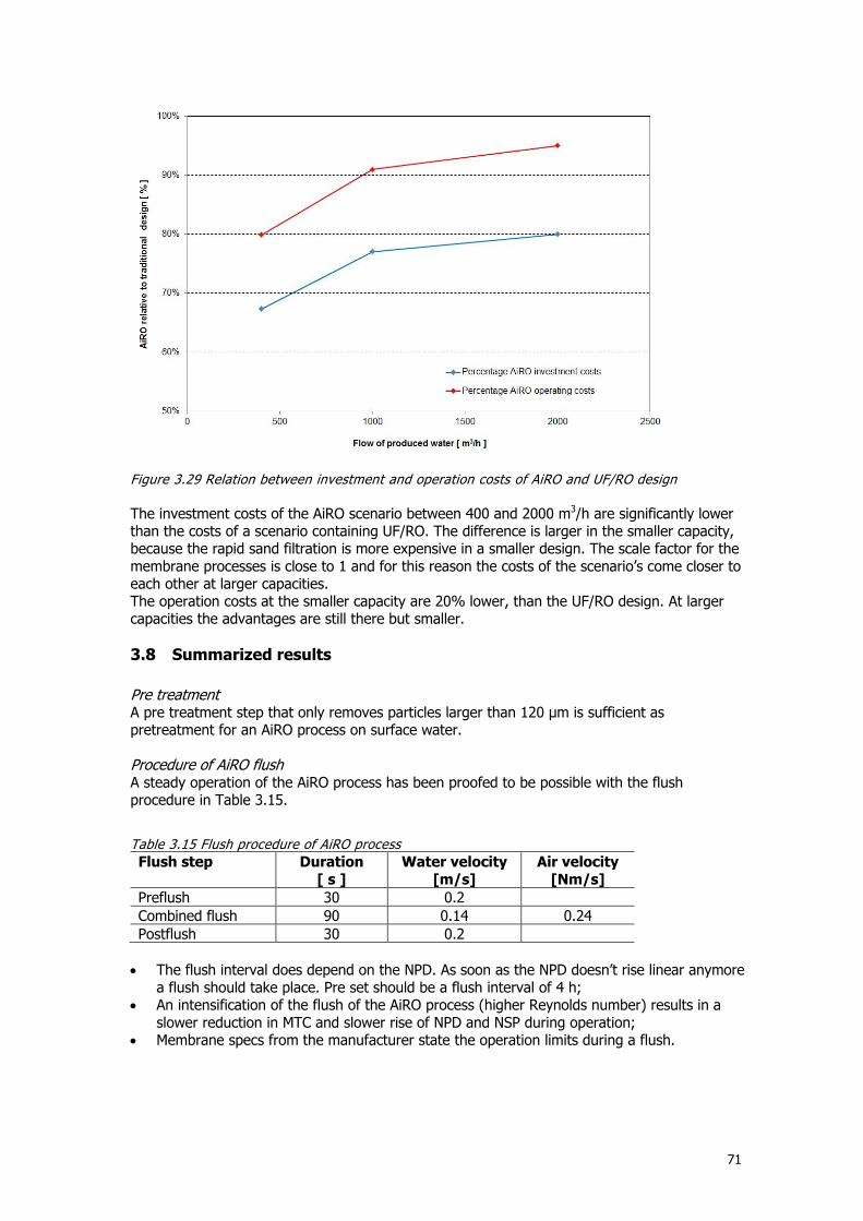
71

Figure 3.29 Relation between investment and operation costs of AiRO and UF/RO design

The investment costs of the AiRO scenario between 400 and 2000 m3/h are significantly lower than the costs of a scenario containing UF/RO. The difference is larger in the smaller capacity, because the rapid sand filtration is more expensive in a smaller design. The scale factor for the membrane processes is close to 1 and for this reason the costs of the scenario’s come closer to each other at larger capacities. The operation costs at the smaller capacity are 20% lower, than the UF/RO design. At larger capacities the advantages are still there but smaller.

3.8 Summarized results

Pre treatment A pre treatment step that only removes particles larger than 120 µm is sufficient as pretreatment for an AiRO process on surface water. Procedure of AiRO flush A steady operation of the AiRO process has been proofed to be possible with the flush procedure in Table 3.15.

Table 3.15 Flush procedure of AiRO process

Flush step Duration [ s ]

Water velocity [m/s]

Air velocity [Nm/s]

Preflush 30 0.2

Combined flush 90 0.14 0.24

Postflush 30 0.2

The flush interval does depend on the NPD. As soon as the NPD doesn’t rise linear anymore

a flush should take place. Pre set should be a flush interval of 4 h; An intensification of the flush of the AiRO process (higher Reynolds number) results in a

slower reduction in MTC and slower rise of NPD and NSP during operation; Membrane specs from the manufacturer state the operation limits during a flush.

72

Feed water quality A variation in turbidity between 4 and 75 FTU did not effect the operation of the AiRO

process during the research; A variation in oxygen content in the feed water, an indication for biological microorganisms,

doesn’t influence the operation of the AiRO process. Chemical cleaning The AiRO process on surface water requires a regular CIP, besides the 4 hourly air/water

flushes; An AiRO treatment on Hollandse IJssel river water requires a CIP with a step for manganese

removal (citric acid or ascorbic acid) and a step for serious TOC removal (by example NC135);

The relation between NPD and passage of a certain salt through the membrane can be a control parameter to adjust the max allowable NPD in the AiRO process;

Economical aspects and plant design The innovative design of an AiRO stack with 2 element pressure vessels and 3” side ports is

fluid mechanical thorough but this stack is more expensive than a traditional stack; The investment costs of a complete drinking water treatment with the AiRO process are 20

to 33% lower than a treatment based on UF and RO; The operation costs of an AiRO treatment are 20 to 5% lower than a traditional UF/RO

treatment.

73

4 Discussion

4.1 Preferable pre treatment

During the Montfoort research, the feed water of the pilot was pretreated with a 120 µm drumfilter. At drinking water treatment plants, the intake of surface water is often provided with rotating drum sieves (also called micro sieves) with a mesh size of 35 µm. They are applied since 1948 and very much is known about the operations of these sieves. They are known as reliable and robust (HWT Waterzuivering, 1977). It’s advised to apply such a treatment step before the AiRO process. The mesh size is smaller than the tested 120 microns mesh size in Montfoort. Advantages are: Less particle load on AiRO process; Protection of the subsequent LD and HD pump; Protection of the Fedco energy recovery unit; Promotes the surge for a solution for the concentrate (concentrate contains less SS and

algae).

4.2 The preflush can be shorter

In § 3.1.2 it is mentioned that a flush consists of the three steps; preflush, combined flush and postflush. Point of discussion is the duration of the preflush. Goal of the preflush is “to wash out the non fixed part of the filtered suspended solids before the combined flush takes place”. Does a flush with only water have advantages above a combined flush? Because the flush energy of a water flush is lower than a combined flush, this is not a reason for selecting a preflush. A plausible reason for choosing a short preflush is to realize a stable water flow before the introduction of the flush air. If both flows start at the same moment (if a preflush is skipped), it’s possible that water and air don’t mix proper. This is undesirable. The preflush will be shorter, the only goal is to maintain a stable water flow before air is introduced. The duration of this preflush have to be determined in practice. The combined flush time will be extended with 30 seconds to maintain at least the same flush energy during a flush.

4.3 Accuracy of economic calculations

An accurate method for determination of the investment costs is to calculate the construction costs of an AiRO stack in detail. This should be done by a construction company and is an impressive amount of work. Too much work for a thesis because for this study an accuracy of ± 30% is sufficient. This is the accuracy of the costing program “CoP Kostencalculatie” [DHV Water, 2009]. But this program doesn’t make a difference between both stack designs. To approximate the difference between the investment costs of a traditional stack and an AiRO stack, only the budget prizes of the pressure vessels are taken into account. In a traditional 200 m3/h, stack the amount of pressure vessels is 39 and the investment costs of the vessels is € 35.000. The budget price for the 105 AiRO pressure vessels with 2 elements inside is € 73.000 [Kalf, 2013]. Just about the price of the vessels, the difference is quite accurate known (± 10%). To make the investment costs comparable in a fair way in the economic calculations in this thesis, it is assumed that the flux in the AiRO stack is half of the flux in the traditional stack. Reducing the flux to half means a two times larger stack with twice as much pressure vessels and twice as much membrane elements. With doubled amount of pressure vessels, the price difference of the pressure vessels is taken into account. The costs of the compensation membrane area is 234 elements x 37 m2/element x 15 €/m2 = € 130.000,-. Is this amount sufficient to finance the design differences between both stacks? Extras to be financed in the AiRO stack are: an air distribution net; a larger feed flow because of the lower recovery in the AiRO unit (larger feed pump and

larger diameter of piping); a flush pump and compressor (they can be applied for more than one stack and those costs

are divided).

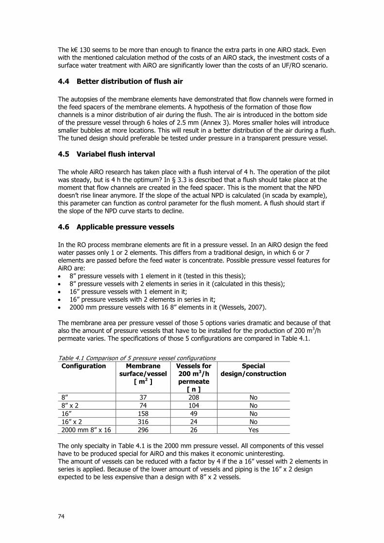
74

The k€ 130 seems to be more than enough to finance the extra parts in one AiRO stack. Even with the mentioned calculation method of the costs of an AiRO stack, the investment costs of a surface water treatment with AiRO are significantly lower than the costs of an UF/RO scenario.

4.4 Better distribution of flush air

The autopsies of the membrane elements have demonstrated that flow channels were formed in the feed spacers of the membrane elements. A hypothesis of the formation of those flow channels is a minor distribution of air during the flush. The air is introduced in the bottom side of the pressure vessel through 6 holes of 2.5 mm (Annex 3). Mores smaller holes will introduce smaller bubbles at more locations. This will result in a better distribution of the air during a flush. The tuned design should preferable be tested under pressure in a transparent pressure vessel.

4.5 Variabel flush interval

The whole AiRO research has taken place with a flush interval of 4 h. The operation of the pilot was steady, but is 4 h the optimum? In § 3.3 is described that a flush should take place at the moment that flow channels are created in the feed spacer. This is the moment that the NPD doesn’t rise linear anymore. If the slope of the actual NPD is calculated (in scada by example), this parameter can function as control parameter for the flush moment. A flush should start if the slope of the NPD curve starts to decline.

4.6 Applicable pressure vessels

In the RO process membrane elements are fit in a pressure vessel. In an AiRO design the feed water passes only 1 or 2 elements. This differs from a traditional design, in which 6 or 7 elements are passed before the feed water is concentrate. Possible pressure vessel features for AiRO are: 8” pressure vessels with 1 element in it (tested in this thesis); 8” pressure vessels with 2 elements in series in it (calculated in this thesis); 16” pressure vessels with 1 element in it; 16” pressure vessels with 2 elements in series in it; 2000 mm pressure vessels with 16 8” elements in it (Wessels, 2007). The membrane area per pressure vessel of those 5 options varies dramatic and because of that also the amount of pressure vessels that have to be installed for the production of 200 m3/h permeate varies. The specifications of those 5 configurations are compared in Table 4.1.

Table 4.1 Comparison of 5 pressure vessel configurations

Configuration Membrane surface/vessel

[ m2 ]

Vessels for 200 m3/h permeate

[ n ]

Special design/construction

8” 37 208 No

8” x 2 74 104 No

16” 158 49 No

16” x 2 316 24 No

2000 mm 8” x 16 296 26 Yes

The only specialty in Table 4.1 is the 2000 mm pressure vessel. All components of this vessel have to be produced special for AiRO and this makes it economic uninteresting. The amount of vessels can be reduced with a factor by 4 if the a 16” vessel with 2 elements in series is applied. Because of the lower amount of vessels and piping is the 16” x 2 design expected to be less expensive than a design with 8” x 2 vessels.

75

If the economical aspects of an AiRO stack with 16” pressure vessels is compared with a traditional surface water treatment, it’s fair that in both designs the 16”pressure vessels should be taken into account. A sufficient distribution of flush air before each element is a crucial issue in each pressure vessel configuration.

4.7 Operational aspects of a 2 element pressure vessel

The economical design is based on a 2 element vertical pressure vessel. This is a theoretic idea, but not tested in practice yet. Why is this idea expected to work? Possible drawbacks of the design are: Problems with the flush Accumulation of debris in dead corners of the pressure vessel Problems with the flush The flush water and air enters the vessel at the bottom and passes both elements before it is disposed. The flush effects at the lower element are the same as in the pilot in Montfoort and this element will for sure be flushed sufficient. For flush air, the upper element is dependent on the flush air distribution in between the elements. This is a serious aspect and the design of the flush air/water distribution plate is crucial (Figure 3.26). The suspended solids content of the flush water that leaves the lower element will contain more SS than the flush water of that vessel. The influence of the SS in the flush water of the upper element is neglectable because in 3.5.1 is concluded that a variation in turbidity has no effect on the operation of the AiRO process. Because the AiRO is flushed with feed water this implicates that turbidity has also no effect on the flush efficiency. The static pressure at bottom of the pressure vessel will be about 30 kPa higher than in a single element vessel. This is neglectable because the pressure in the vessel at the moment of a flush is 345 kPa max. Accumulation of debris in dead corners of the pressure vessel The top and bottom construction in a 2 element vessel is not differentiated compared to the single element pressure vessel. The middle part with the air/water distribution plate is new. During the AiRO research in Montfoort 2 pressure vessels have been dismantled to remove the elements for an autopsy. In this dismantling operation is observed that no debris was accumulated in dead corners. Obvious the turbulence that the in steaming feed water and flush water and air causes is thus high that the dead corners are kept clean. This turbulence will also occur in the space with the distribution plate between the elements and for this reason no accumulation of debris is expected in the dead corners.

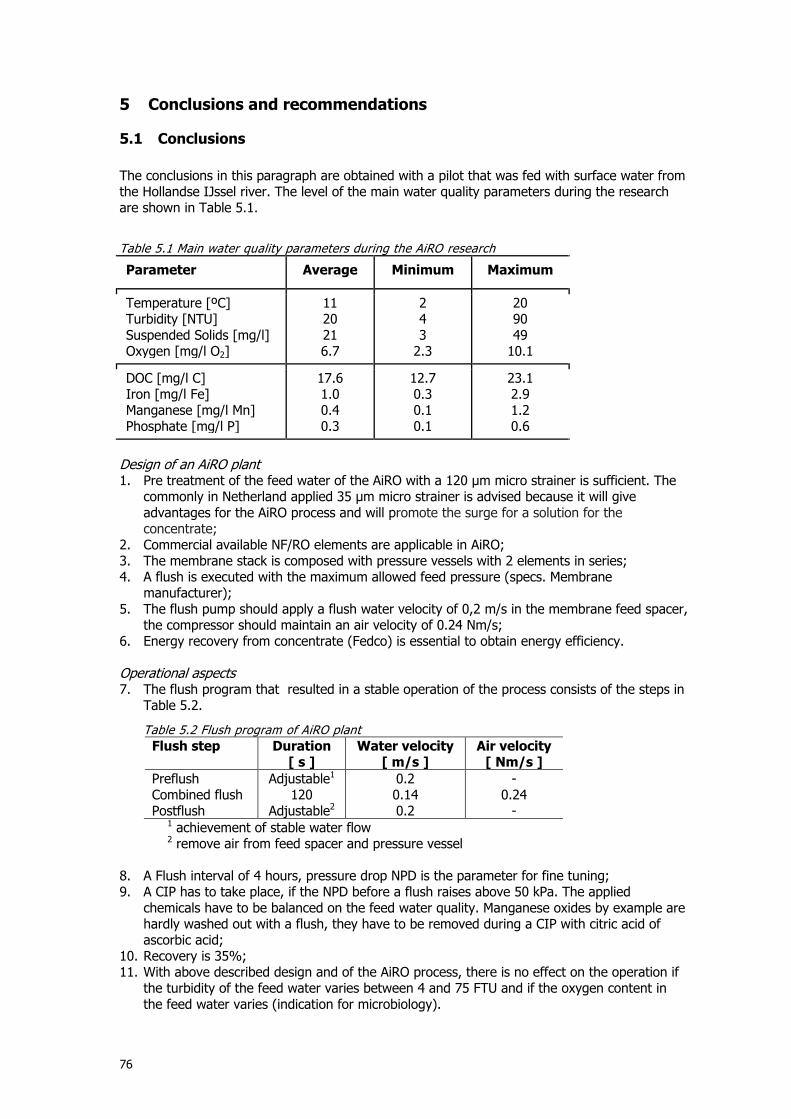
76

5 Conclusions and recommendations

5.1 Conclusions

The conclusions in this paragraph are obtained with a pilot that was fed with surface water from the Hollandse IJssel river. The level of the main water quality parameters during the research are shown in Table 5.1.

Table 5.1 Main water quality parameters during the AiRO research

Parameter Average Minimum Maximum

Temperature [ºC] Turbidity [NTU] Suspended Solids [mg/l] Oxygen [mg/l O2]

11 20 21 6.7

2 4 3

2.3

20 90 49

10.1

DOC [mg/l C] Iron [mg/l Fe] Manganese [mg/l Mn] Phosphate [mg/l P]

17.6 1.0 0.4 0.3

12.7 0.3 0.1 0.1

23.1 2.9 1.2 0.6

Design of an AiRO plant 1. Pre treatment of the feed water of the AiRO with a 120 µm micro strainer is sufficient. The

commonly in Netherland applied 35 µm micro strainer is advised because it will give advantages for the AiRO process and will promote the surge for a solution for the concentrate;

2. Commercial available NF/RO elements are applicable in AiRO; 3. The membrane stack is composed with pressure vessels with 2 elements in series; 4. A flush is executed with the maximum allowed feed pressure (specs. Membrane

manufacturer); 5. The flush pump should apply a flush water velocity of 0,2 m/s in the membrane feed spacer,

the compressor should maintain an air velocity of 0.24 Nm/s; 6. Energy recovery from concentrate (Fedco) is essential to obtain energy efficiency. Operational aspects 7. The flush program that resulted in a stable operation of the process consists of the steps in

Table 5.2.

Table 5.2 Flush program of AiRO plant

Flush step Duration [ s ]

Water velocity [ m/s ]

Air velocity [ Nm/s ]

Preflush Combined flush Postflush

Adjustable1 120

Adjustable2

0.2 0.14 0.2

- 0.24

- 1 achievement of stable water flow 2 remove air from feed spacer and pressure vessel

8. A Flush interval of 4 hours, pressure drop NPD is the parameter for fine tuning; 9. A CIP has to take place, if the NPD before a flush raises above 50 kPa. The applied

chemicals have to be balanced on the feed water quality. Manganese oxides by example are hardly washed out with a flush, they have to be removed during a CIP with citric acid of ascorbic acid;

10. Recovery is 35%; 11. With above described design and of the AiRO process, there is no effect on the operation if

the turbidity of the feed water varies between 4 and 75 FTU and if the oxygen content in the feed water varies (indication for microbiology).

77

Concentrate en rest streams 12. Operation of AiRO at low recovery results in a large concentrate stream, that free is of

antiscalant with a low content of salts. This flow is expected to be allowed to discharge to surface water;

13. The flush water can be discharged to surface water, after sedimentation of the solids in it; 14. The produced sludge is free of chemical additions. This will improve the useful application of

the sludge; 15. The used CIP fluid has to be discharged to the sewer after neutralisation of the pH. Economical aspects If an AiRO stack design with pressure vessels that contains 2 elements is taken into account, can be concluded that: 16. The investment costs of a complete drinking water treatment with the AiRO process are 20

to 33% lower than a treatment based on UF and RO; 17. The operation costs of an AiRO treatment are 20 to 5% lower than a traditional UF/RO

treatment. The application of 16” pressure vessels containing 2 16” elements in series, may result in lower investment costs. Overall conclusions concerning AiRO 18. Is a reliable barrier in a surface water purification process line; 19. Is a robust process; 20. Uses a limited amount of chemicals; 21. Is economic interesting; 22. AiRO withstood the practical durability test.

5.2 Recommendations

Recommendations for further research are: 1. The calculations of the economical aspects are based on a stack design with pressure

vessels containing 2 elements in series. This is a theoretical design that is expected to be reliable but is not tested in practice yet. For this reason a long term research on surface water with an AiRO pilot provided with a 2 element pressure vessel is advised.

2. In this research 2 water and air flush ratios are investigated. The operation of the pilot was steady with the tested ratios but a different air/water flush ratio may have a different effect. Further research on this operational aspect is recommended.

3. Reliable construction costs calculations of an AiRO stack are not available yet. A better estimation of the construction costs will results in more reliable comparison of the economics of an AiRO treatment with a traditional treatment.

78

List of references

Bennett A.: 2009 Pathogen removal from water – technologies and techniques Filtration and

Separation online

Bereschenko, L.A.: (2010) Biofilm development on new and cleaned membrane surfaces Thesis, Wageningen University, Wageningen, NL

Cheng, T.W., Li, L.N.: (2007) Gas-sparging cross-flow ultrafiltration in flat-plate membrane

module: effects of channel height and membrane inclination Separation and Purification Technology 55 (2007) 50.

Cornelissen, E (2006) Membraanreiniging van NF/RO installaties, Een literatuurstudie KWR BTO

2005.060 juni 2006 Cornelissen E.R., Vrouwenvelder J.S., Heijman S.G.J., Viallefont X.D., Van der Kooij D., Wessels

L.P.: (2007) Periodic air/water cleaning for control of biofouling in spiral wound membrane elements Journal of Membrane Science 287 (2007) 94-101

Cornelissen, E.R., Rebour, L, Kooij, D. van der, Wessels, L.P.: (2009) Optimization of air/water

cleaning (AWC) in spiral wound elements. Desalination, 2009. 236(1-3): p. 266-272. Cornelissen E.R., Viallefont X.D., Beerendonk E.F., Wessels L.P.: (2009) Air/water cleaning for

the control of particulate fouling Water Science and Technology DHV Water BV: June 2009 CoP Kostencalculatie, Niveau beleidsplan en systeemkeuze,

Drinkwater dossier A6745-02-001 versie 6 Fedco: (2012) Product & Applications Catalog 2012 HP Feed Pumps and Energy Recovery

Boosters for Brackish Water and Seawater RO Applications Flemming, H.-C., G. Schaule, T. Griebe, J. Schmitt, A. Tamachkiarowa: (1997) Biofouling - the

Achilles heel of membrane processes Desalination 113: 215-225 Huiting, H., Koning, M. de, Beerendonk, E.F.: 1999 Normalisatie van gegevens bij nanofiltratie

en omgekeerde osmose KWR/BTO SWI 99.166 Haidari, A.: (2011) Real time Visualization of membrane poster Department Water

Management, Section Sanitary Engineering, Delft University of Technology, Netherlands Hatenboer-Water: oktober 2010 Handleiding AiRO pilot installatie project 435199 Hijnen, W.A.M., Biraud, D., Cornelissen, E.R., Van der Koo , D. 2009. Threshold concentration of

easily assimilable organic carbon in feedwater for biofouling of spiral-wound membranes. Environmental Science and Technology 43: 4890-4895

Hoek, J.P. van der, Hofman, J.A.M.H., Bonné, P.A.C., Nederlof, M.M., Vrouwenvelder, H.S.:

(2000) RO treatment: Selection of a pretreatment scheme based on fouling characteristics and operating conditions based on environmental impact Desalination 127: 89-101.

Hyppönen, H.: (2008) Treatment of surface water with hydraulically cleaned reverse osmosis

modules Bachelor's thesis Environmental technology HAMK University of applied science IWA publishing: (2012) See who’s made a splash, IWA Project Innovation Awards Water 21 Jong, R.C.M., Nederlof, M.M.: (2003) Results of Elsbeekweg biocide research WMO

79

Jong, R.C.M.: (2006) Ervaringen bij Vitens met lozing van membraanconcentraat In: H2O Jong, R.C.M. (2007). Voordelen van een RO stack ontwerp met centre port drukvaten In: NPT

Procestechniek Kooij, D. van der: (1992) Assimilable organic carbon as an indicator of bacterial regrowth. J. Am.

Water Works Assoc. 84: 57-65. Kalf, M: Budget prices of pressure vessels, Logisticon mail dd 2013-07-16 Meer, W.G.J. van der, Paassen, J.A.M. van, Riemersma, M.C., Ekkendonk F.H.J. (2003)

OPTIFLUX®: From Innovation to Realisation presented at the European Conference on Desalination and the Environment Fresh water for all, may 4-8, 2003 Malta

Mulder, M.: (1991) Basic Principles of Membrane Technology Kluwer ISBN 0-7923-0979-0 Ngene, I.S., Lammertink, R.G.H., Kemperman, A.J.B., Van de Ven, W.J.C., Wessels, L.P.,

Wessling, M., Van der Meer, W.G.J. (2010) CO2 Nucleation in Membrane Spacer Channel

Remove Biofilms and Fouling Deposits Industrial & Engineering Chemistry Research: 49, 10034-10039

Pot, M., Berg, R. van den, Agtmaal, J. van; (2011) DWP Botlek - largest demin water plant in

the Netherlands 6th IWA Specialist Conference on Membrane Technology for Water & Wastewater Treatment Aachen

Rietman, B.M.: (2006) Anaerobic nanofiltration in drinking water production, 7 years successful

operation Workshop Techneau, December 14 2006 Rietman, B.M.: (2013) Clean Operator, Cleaning spiral wound membrane modules with a two

phase solution Thesis for the degree of: Master of Science in Civil Engineering, Delft University of Technology

Shakaib, M., Hasani, S.M.F., Mahmood, M. (2007) Study on the effects of spacer geometry in

membrane feed channels using three-dimensional computational flow modeling Journal of Membrane Science Volume 297, Issues 1–2, 5 July 2007, Pages 74–89

TriSep Reverse Osmosis Implementation program TROI version 2.5.0 www.trisep.com Trisep Recommended Cleaning Conditions http://membranes.trisep.com/ Verliefde, Arne R.D. (2008) Rejection of organic micropollutants by high pressure membranes

(NF/RO). Thesis TU-Delft, Vrouwenvelder, J.S., Bakker, S.M., Cauchard, M., Le Grand, R., Apacandie, M., Idrissi, M.,

Lagrave, S., Wessels, L.P., Van Paassen, J.A.M., Kruithof, J.C., Van Loosdrecht, M.C.M. (2007) The membrane fouling simulator: a suitable tool for prediction and characterization of membrane fouling Water Science & Technology Vol 55 No 8–9 pp 197–205 Q IWA Publishing 2007

Vrouwenvelder, J.S., (2009) Biofouling of spiral wound membrane systems

PhD thesis Delft University of Technology Wessels, L.P., Jong, R.C.M., Rietman, B.M.: (2001) Werkwijze en inrichting voor het zuiveren

van oppervlaktewater Octrooi NL C 101 9130 dd 8-10-2001 Wessels, P., Heijman, B., Viallefont, X., Cornelissen, E.: (2006) Nieuwe aanpak

membraanvervuiling reinigen met lucht en water Platform artikel H2O

80

Wessels, P., Heijman, B., Cornelissen, E.: (2007) Apparatus for purification of water and a

method for its use WO Patent 2007/043879 A1 Wibisono, Y.: (2010) AiRO, The Use of Two Phase Flow in Controlling Fouling in Spiral Wound

Membranes PhD. In Membrane Technology Group, University of Twente, Netherlands Willems, P., Kemperman, A.J.B., Lammertink, R.G.H., Wessling, M., Sint Annaland, M. van,

Deen, N.G., Kuipers, J.A.M., Meer, W.G.J. van der (2009) Bubbles in spacers: Direct observation of bubble behavior in spacer filled membrane channels Journal of Membrane Science, 333 (1-2). pp. 38-44

Patching, J. W., Fleming, G. T. A.: (2003) Industrial biofilms: Formation, problems and control in:

Lens, P., A.P. Moran, T. Mahony, P. Stoodley, and V. O’Flaherty (ed.). Biofilms in medicine, industry and environmental biotechnology IWA publishing. UK. 568-572.

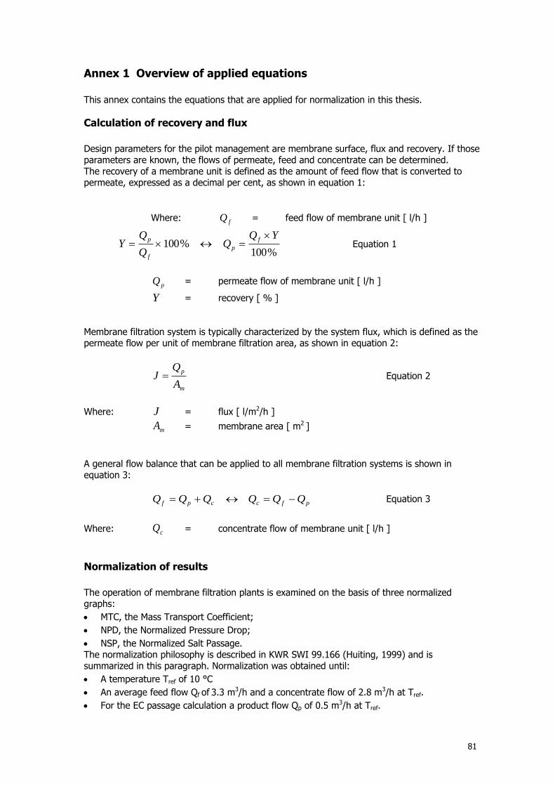
81

Annex 1 Overview of applied equations

This annex contains the equations that are applied for normalization in this thesis.

Calculation of recovery and flux

Design parameters for the pilot management are membrane surface, flux and recovery. If those parameters are known, the flows of permeate, feed and concentrate can be determined. The recovery of a membrane unit is defined as the amount of feed flow that is converted to permeate, expressed as a decimal per cent, as shown in equation 1:

Where: fQ = feed flow of membrane unit [ l/h ]

%100%100

YQQ

Q

QY

f

p

f

p Equation 1

pQ = permeate flow of membrane unit [ l/h ]

Y = recovery [ % ] Membrane filtration system is typically characterized by the system flux, which is defined as the permeate flow per unit of membrane filtration area, as shown in equation 2:

m

p

A

QJ Equation 2

Where: J = flux [ l/m2/h ]

mA = membrane area [ m2 ]

A general flow balance that can be applied to all membrane filtration systems is shown in equation 3:

pfccpf QQQQQQ Equation 3

Where: cQ = concentrate flow of membrane unit [ l/h ]

Normalization of results

The operation of membrane filtration plants is examined on the basis of three normalized graphs:

MTC, the Mass Transport Coefficient;

NPD, the Normalized Pressure Drop;

NSP, the Normalized Salt Passage. The normalization philosophy is described in KWR SWI 99.166 (Huiting, 1999) and is summarized in this paragraph. Normalization was obtained until:

A temperature Tref of 10 °C

An average feed flow Qf of 3.3 m3/h and a concentrate flow of 2.8 m3/h at Tref.

For the EC passage calculation a product flow Qp of 0.5 m3/h at Tref.

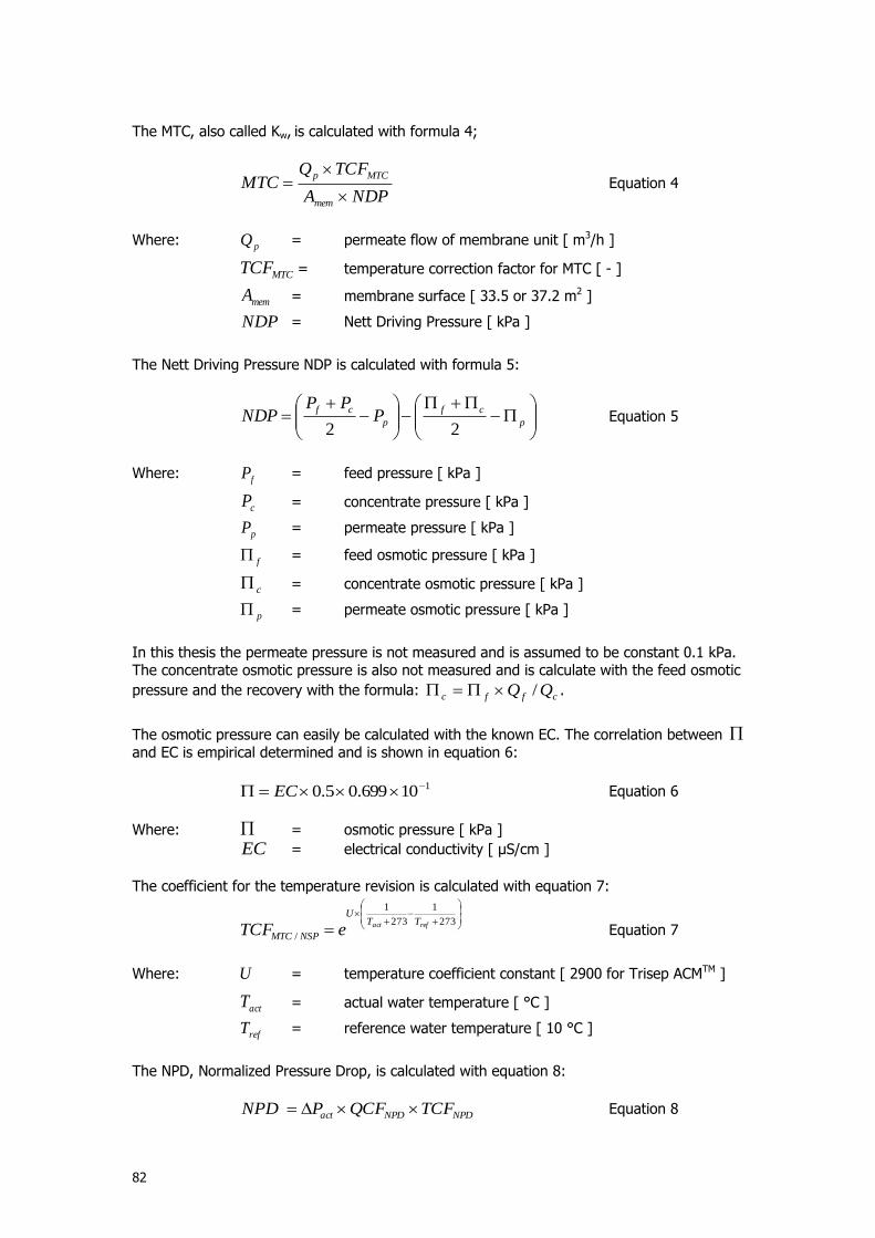
82

The MTC, also called Kw, is calculated with formula 4;

NDPA

TCFQMTC

mem

MTCp

Equation 4

Where: pQ = permeate flow of membrane unit [ m3/h ]

MTCTCF = temperature correction factor for MTC [ - ]

memA = membrane surface [ 33.5 or 37.2 m2 ]

NDP = Nett Driving Pressure [ kPa ]

The Nett Driving Pressure NDP is calculated with formula 5:

p

cf

p

cfP

PPNDP

22 Equation 5

Where: fP = feed pressure [ kPa ]

cP = concentrate pressure [ kPa ]

pP = permeate pressure [ kPa ]

f = feed osmotic pressure [ kPa ]

c = concentrate osmotic pressure [ kPa ]

p = permeate osmotic pressure [ kPa ]

In this thesis the permeate pressure is not measured and is assumed to be constant 0.1 kPa. The concentrate osmotic pressure is also not measured and is calculate with the feed osmotic

pressure and the recovery with the formula: cffc QQ / .

The osmotic pressure can easily be calculated with the known EC. The correlation between and EC is empirical determined and is shown in equation 6:

110699.05.0 EC Equation 6

Where: = osmotic pressure [ kPa ]

EC = electrical conductivity [ µS/cm ]

The coefficient for the temperature revision is calculated with equation 7:

273

1

273

1

/

refact TTU

NSPMTC eTCF Equation 7

Where: U = temperature coefficient constant [ 2900 for Trisep ACMTM ]

actT = actual water temperature [ °C ]

refT = reference water temperature [ 10 °C ]

The NPD, Normalized Pressure Drop, is calculated with equation 8:

NPDNPDact TCFQCFPNPD Equation 8

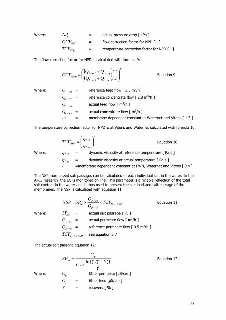
83

Where: actP = actual pressure drop [ kPa ]

NPDQCF = flow correction factor for NPD [ - ]

NPDTCF = temperature correction factor for NPD [ - ]

The flow correction factor for NPD is calculated with formula 9:

m

actcactf

refcreff

NDPQQ

QQQCF

2/

2/ Equation 9

Where: reffQ = reference feed flow [ 3.3 m3/h ]

refcQ = reference concentrate flow [ 2.8 m3/h ]

actfQ = actual feed flow [ m3/h ]

actcQ = actual concentrate flow [ m3/h ]

m = membrane dependent constant at Waternet and Vitens [ 1.5 ]

The temperature correction factor for NPD is at Vitens and Waternet calculated with formula 10:

n

Tact

Tref

NDPTCF

Equation 10

Where: Tref = dynamic viscosity at reference temperature [ Pa.s ]

Tact = dynamic viscosity at actual temperature [ Pa.s ]

n =membrane dependent constant at PWN, Waternet and Vitens [ 0.4 ]

The NSP, normalized salt passage, can be calculated of each individual salt in the water. In the AiRO research the EC is monitored on line. This parameter is a reliable reflection of the total salt content in the water and is thus used to present the salt load and salt passage of the membranes. The NSP is calculated with equation 11:

NSPMTC

refp

actp

act TCFQ

QSPNSP /

Equation 11

Where: actSP = actual salt passage [ % ]

actpQ = actual permeate flow [ m3/h ]

refpQ = reference permeate flow [ 0.5 m3/h ]

NSPMTCTCF / = see equation 3.7

The actual salt passage equation 12:

Y

YC

CSP

f

p

act )}1/(1ln{(

Equation 12

Where: pC = EC of permeate [µS/cm ]

fC = EC of feed [µS/cm ]

Y = recovery [ % ]

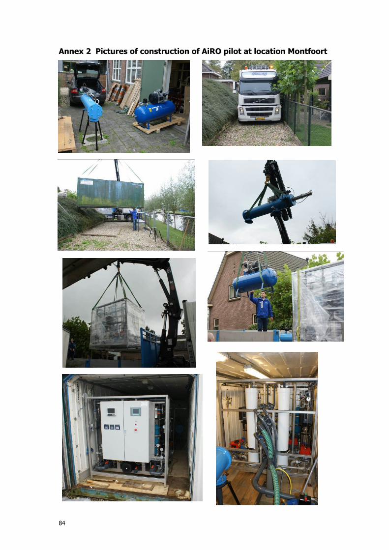
84

Annex 2 Pictures of construction of AiRO pilot at location Montfoort

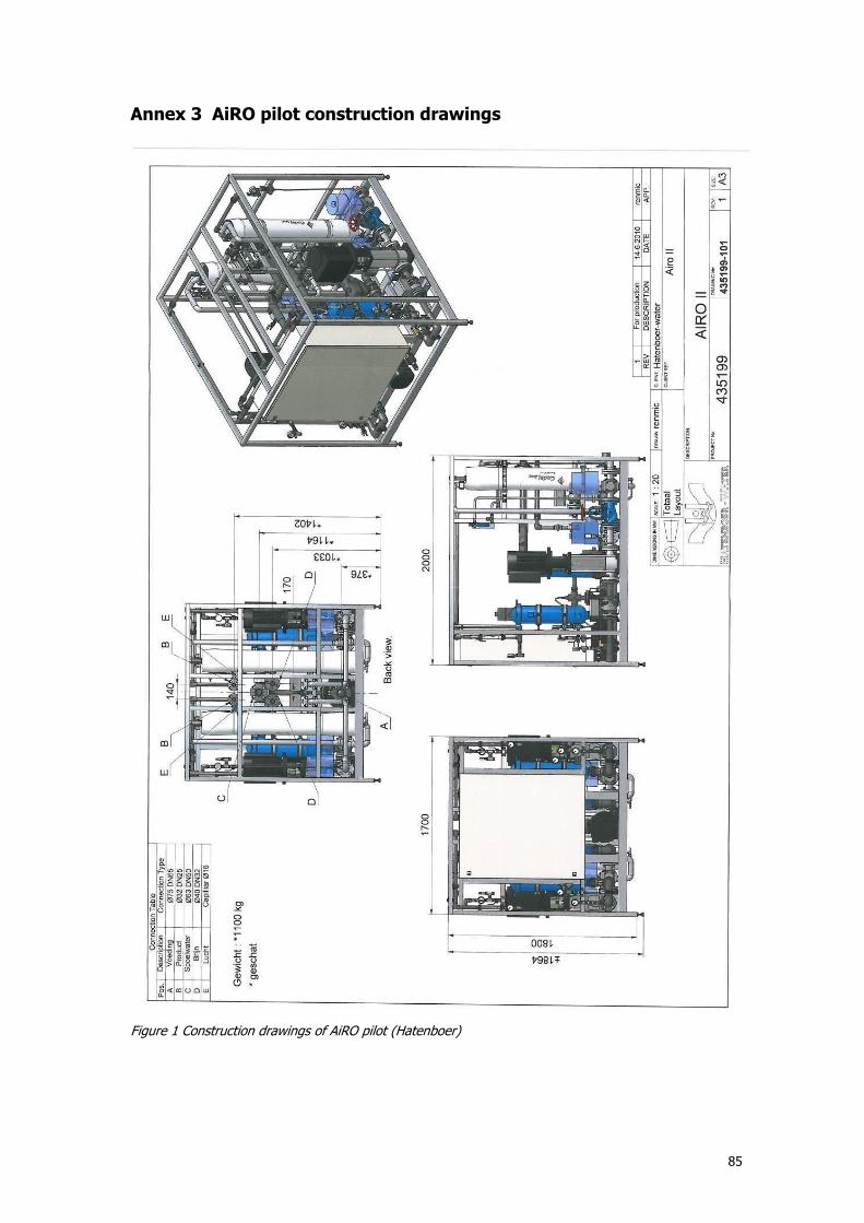
85

Annex 3 AiRO pilot construction drawings

Figure 1 Construction drawings of AiRO pilot (Hatenboer)

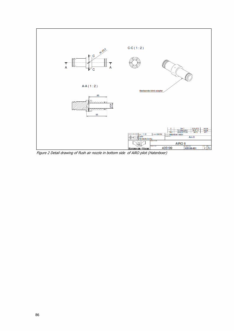
86

Figure 2 Detail drawing of flush air nozzle in bottom side of AiRO pilot (Hatenboer)

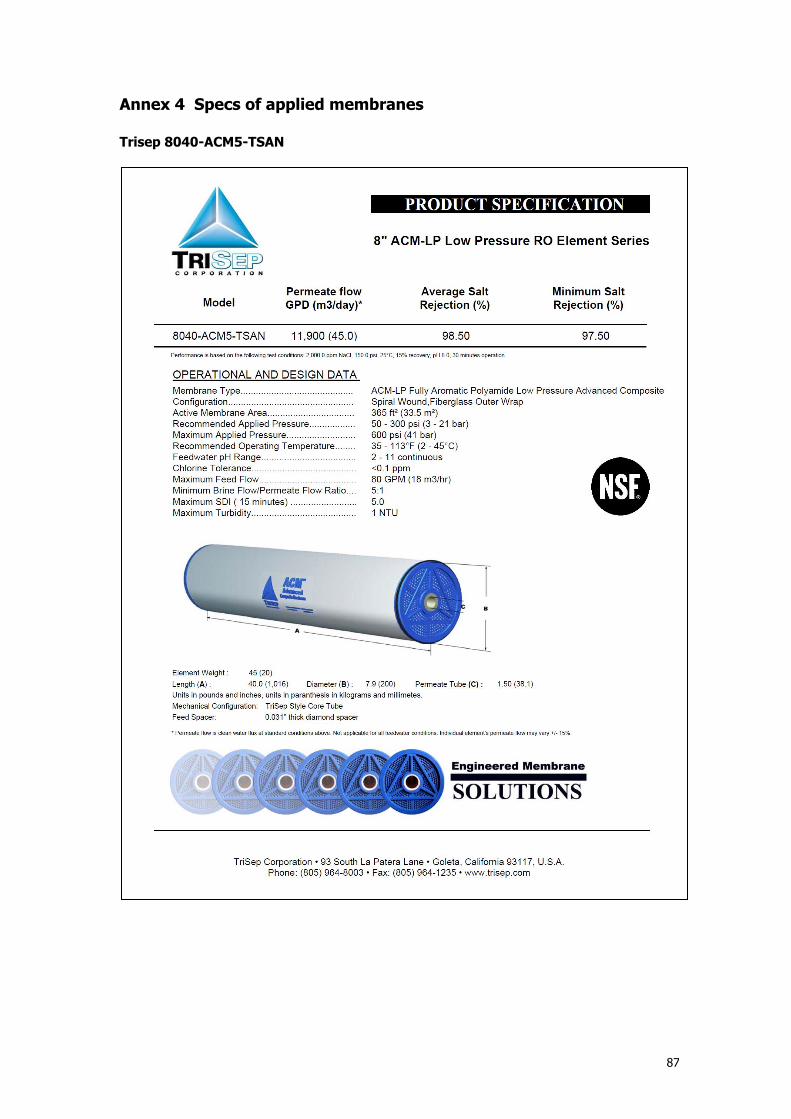
87

Annex 4 Specs of applied membranes

Trisep 8040-ACM5-TSAN

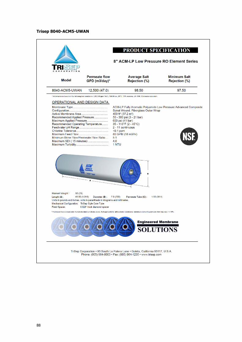
88

Trisep 8040-ACM5-UWAN

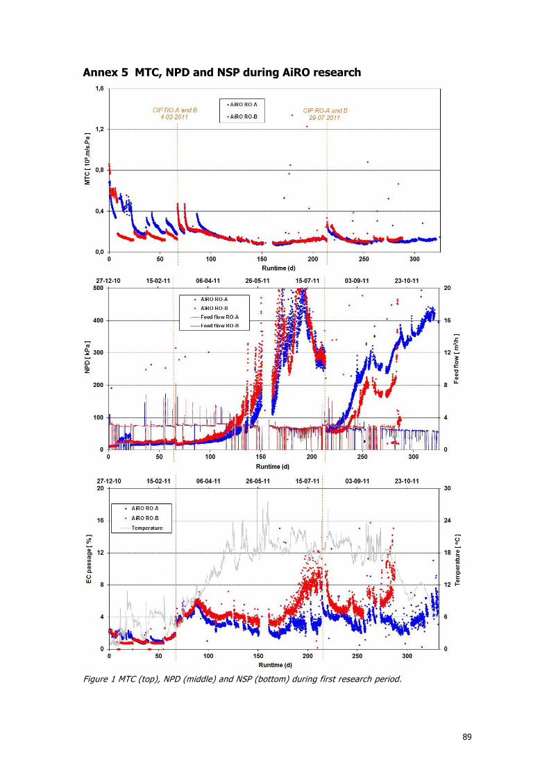
89

Annex 5 MTC, NPD and NSP during AiRO research

Figure 1 MTC (top), NPD (middle) and NSP (bottom) during first research period.

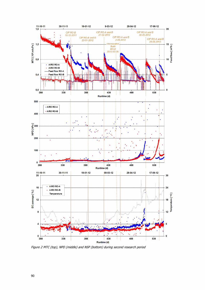
90

Figure 2 MTC (top), NPD (middle) and NSP (bottom) during second research period

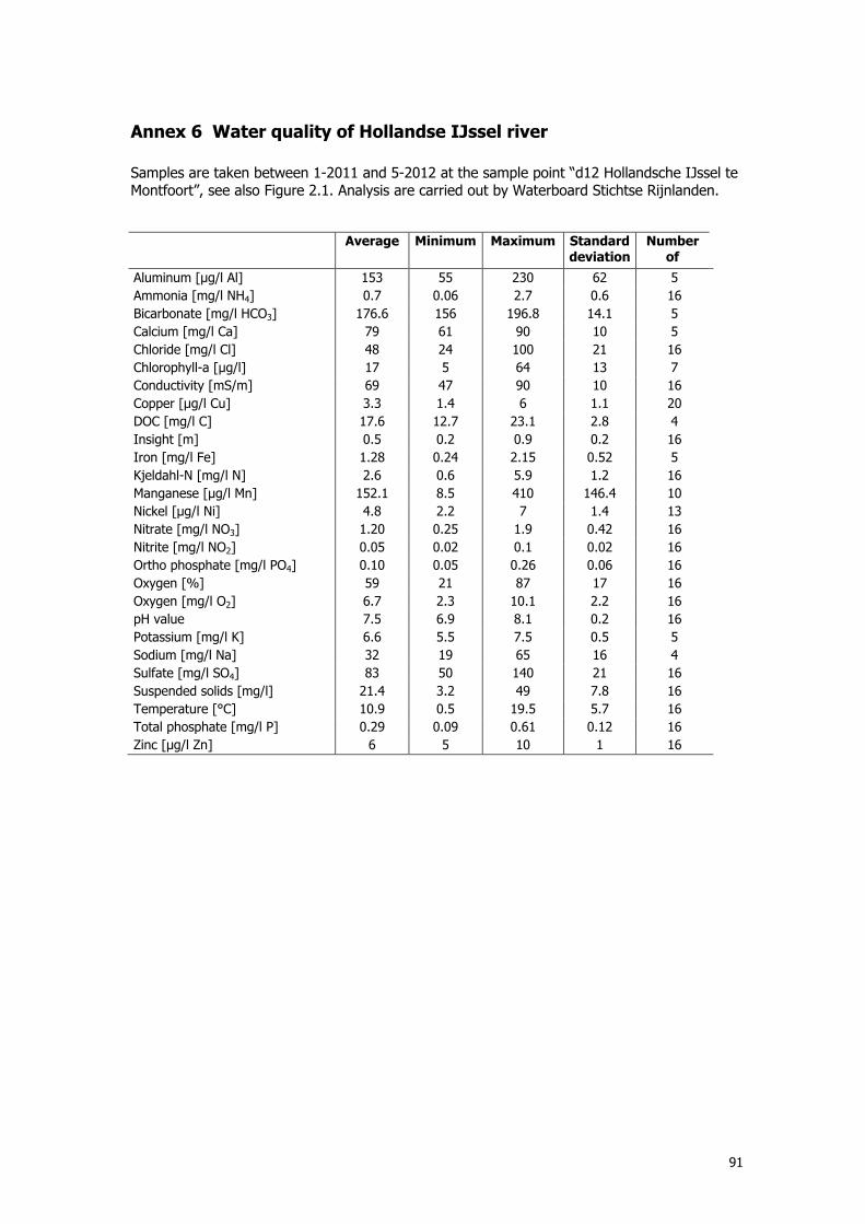
91

Annex 6 Water quality of Hollandse IJssel river

Samples are taken between 1-2011 and 5-2012 at the sample point “d12 Hollandsche IJssel te Montfoort”, see also Figure 2.1. Analysis are carried out by Waterboard Stichtse Rijnlanden.

Average Minimum Maximum Standard deviation

Number of

Aluminum [µg/l Al] 153 55 230 62 5

Ammonia [mg/l NH4] 0.7 0.06 2.7 0.6 16

Bicarbonate [mg/l HCO3] 176.6 156 196.8 14.1 5

Calcium [mg/l Ca] 79 61 90 10 5

Chloride [mg/l Cl] 48 24 100 21 16

Chlorophyll-a [µg/l] 17 5 64 13 7

Conductivity [mS/m] 69 47 90 10 16

Copper [µg/l Cu] 3.3 1.4 6 1.1 20

DOC [mg/l C] 17.6 12.7 23.1 2.8 4

Insight [m] 0.5 0.2 0.9 0.2 16

Iron [mg/l Fe] 1.28 0.24 2.15 0.52 5

Kjeldahl-N [mg/l N] 2.6 0.6 5.9 1.2 16

Manganese [µg/l Mn] 152.1 8.5 410 146.4 10

Nickel [µg/l Ni] 4.8 2.2 7 1.4 13

Nitrate [mg/l NO3] 1.20 0.25 1.9 0.42 16

Nitrite [mg/l NO2] 0.05 0.02 0.1 0.02 16

Ortho phosphate [mg/l PO4] 0.10 0.05 0.26 0.06 16

Oxygen [%] 59 21 87 17 16

Oxygen [mg/l O2] 6.7 2.3 10.1 2.2 16

pH value 7.5 6.9 8.1 0.2 16

Potassium [mg/l K] 6.6 5.5 7.5 0.5 5

Sodium [mg/l Na] 32 19 65 16 4

Sulfate [mg/l SO4] 83 50 140 21 16

Suspended solids [mg/l] 21.4 3.2 49 7.8 16

Temperature [°C] 10.9 0.5 19.5 5.7 16

Total phosphate [mg/l P] 0.29 0.09 0.61 0.12 16

Zinc [µg/l Zn] 6 5 10 1 16

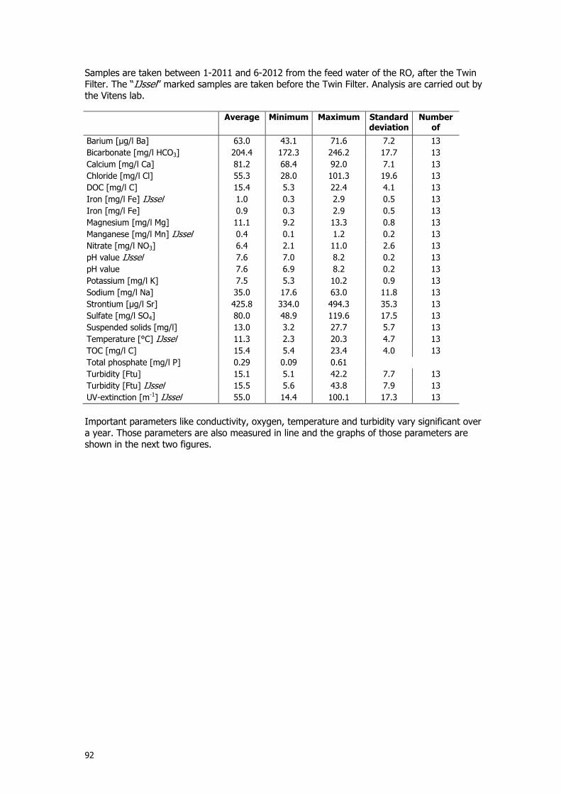
92

Samples are taken between 1-2011 and 6-2012 from the feed water of the RO, after the Twin Filter. The “IJssel” marked samples are taken before the Twin Filter. Analysis are carried out by the Vitens lab.

Average Minimum Maximum Standard deviation

Number of

Barium [µg/l Ba] 63.0 43.1 71.6 7.2 13

Bicarbonate [mg/l HCO3] 204.4 172.3 246.2 17.7 13

Calcium [mg/l Ca] 81.2 68.4 92.0 7.1 13

Chloride [mg/l Cl] 55.3 28.0 101.3 19.6 13

DOC [mg/l C] 15.4 5.3 22.4 4.1 13

Iron [mg/l Fe] IJssel 1.0 0.3 2.9 0.5 13

Iron [mg/l Fe] 0.9 0.3 2.9 0.5 13

Magnesium [mg/l Mg] 11.1 9.2 13.3 0.8 13

Manganese [mg/l Mn] IJssel 0.4 0.1 1.2 0.2 13

Nitrate [mg/l NO3] 6.4 2.1 11.0 2.6 13

pH value IJssel 7.6 7.0 8.2 0.2 13

pH value 7.6 6.9 8.2 0.2 13

Potassium [mg/l K] 7.5 5.3 10.2 0.9 13

Sodium [mg/l Na] 35.0 17.6 63.0 11.8 13

Strontium [µg/l Sr] 425.8 334.0 494.3 35.3 13

Sulfate [mg/l SO4] 80.0 48.9 119.6 17.5 13

Suspended solids [mg/l] 13.0 3.2 27.7 5.7 13

Temperature [°C] IJssel 11.3 2.3 20.3 4.7 13

TOC [mg/l C] 15.4 5.4 23.4 4.0 13

Total phosphate [mg/l P] 0.29 0.09 0.61

Turbidity [Ftu] 15.1 5.1 42.2 7.7 13

Turbidity [Ftu] IJssel 15.5 5.6 43.8 7.9 13

UV-extinction [m-1] IJssel 55.0 14.4 100.1 17.3 13

Important parameters like conductivity, oxygen, temperature and turbidity vary significant over a year. Those parameters are also measured in line and the graphs of those parameters are shown in the next two figures.

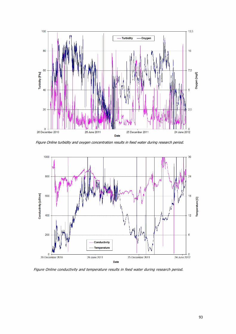
93

Figure Online conductivity and temperature results in feed water during research period.

Figure Online turbidity and oxygen concentration results in feed water during research period.

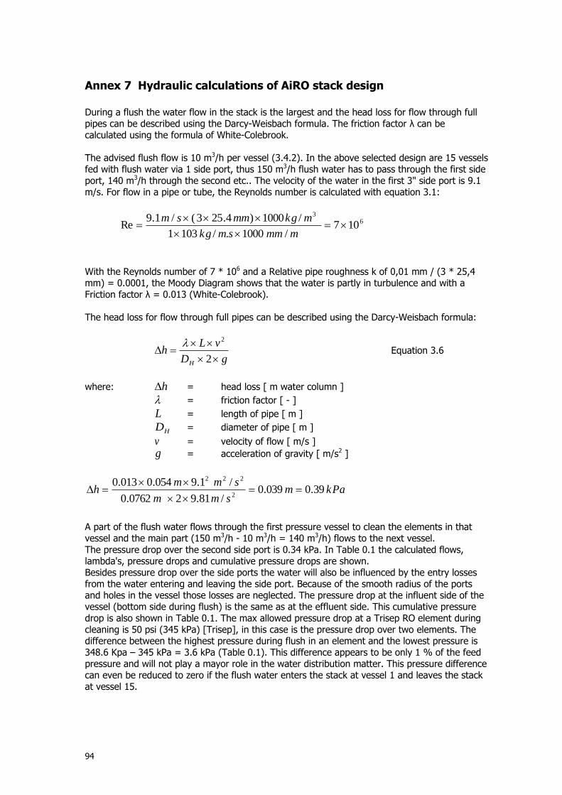
94

Annex 7 Hydraulic calculations of AiRO stack design

During a flush the water flow in the stack is the largest and the head loss for flow through full pipes can be described using the Darcy-Weisbach formula. The friction factor λ can be calculated using the formula of White-Colebrook. The advised flush flow is 10 m3/h per vessel (3.4.2). In the above selected design are 15 vessels fed with flush water via 1 side port, thus 150 m3/h flush water has to pass through the first side port, 140 m3/h through the second etc.. The velocity of the water in the first 3" side port is 9.1 m/s. For flow in a pipe or tube, the Reynolds number is calculated with equation 3.1:

63

107/1000./1031

/1000)4.253(/1.9Re

mmmsmkg

mkgmmsm

With the Reynolds number of 7 * 106 and a Relative pipe roughness k of 0,01 mm / (3 * 25,4 mm) = 0.0001, the Moody Diagram shows that the water is partly in turbulence and with a Friction factor λ = 0.013 (White-Colebrook). The head loss for flow through full pipes can be described using the Darcy-Weisbach formula:

gD

vLh

H

2

2 Equation 3.6

where: h = head loss [ m water column ]

= friction factor [ - ]

L = length of pipe [ m ]

HD = diameter of pipe [ m ]

v = velocity of flow [ m/s ]

g = acceleration of gravity [ m/s2 ]

kPamsmm

smmh 39.0039.0

/81.920762.0

/1.9054.0013.02

222

A part of the flush water flows through the first pressure vessel to clean the elements in that vessel and the main part (150 m3/h - 10 m3/h = 140 m3/h) flows to the next vessel. The pressure drop over the second side port is 0.34 kPa. In Table 0.1 the calculated flows, lambda's, pressure drops and cumulative pressure drops are shown. Besides pressure drop over the side ports the water will also be influenced by the entry losses from the water entering and leaving the side port. Because of the smooth radius of the ports and holes in the vessel those losses are neglected. The pressure drop at the influent side of the vessel (bottom side during flush) is the same as at the effluent side. This cumulative pressure drop is also shown in Table 0.1. The max allowed pressure drop at a Trisep RO element during cleaning is 50 psi (345 kPa) [Trisep], in this case is the pressure drop over two elements. The difference between the highest pressure during flush in an element and the lowest pressure is 348.6 Kpa – 345 kPa = 3.6 kPa (Table 0.1). This difference appears to be only 1 % of the feed pressure and will not play a mayor role in the water distribution matter. This pressure difference can even be reduced to zero if the flush water enters the stack at vessel 1 and leaves the stack at vessel 15.

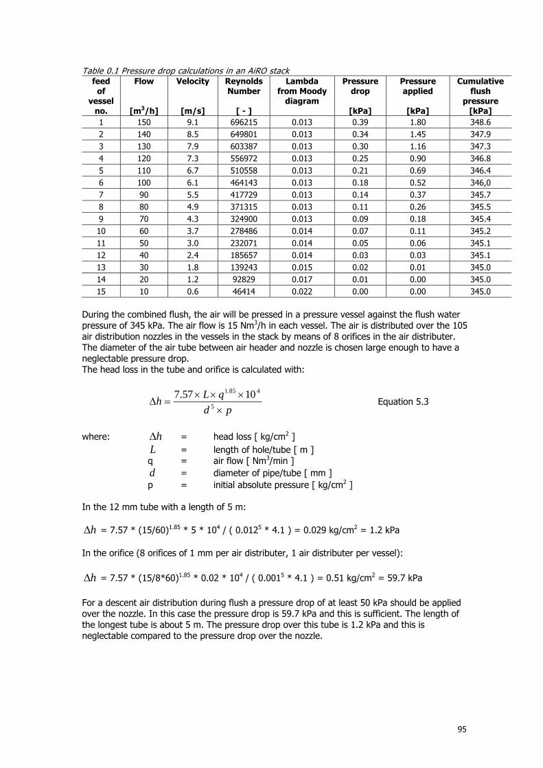
95

Table 0.1 Pressure drop calculations in an AiRO stack feed

of vessel

no.

Flow

[m3/h]

Velocity

[m/s]

Reynolds Number

[ - ]

Lambda from Moody

diagram

Pressure drop

[kPa]

Pressure applied

[kPa]

Cumulative flush

pressure [kPa]

1 150 9.1 696215 0.013 0.39 1.80 348.6

2 140 8.5 649801 0.013 0.34 1.45 347.9

3 130 7.9 603387 0.013 0.30 1.16 347.3

4 120 7.3 556972 0.013 0.25 0.90 346.8

5 110 6.7 510558 0.013 0.21 0.69 346.4

6 100 6.1 464143 0.013 0.18 0.52 346,0

7 90 5.5 417729 0.013 0.14 0.37 345.7

8 80 4.9 371315 0.013 0.11 0.26 345.5

9 70 4.3 324900 0.013 0.09 0.18 345.4

10 60 3.7 278486 0.014 0.07 0.11 345.2

11 50 3.0 232071 0.014 0.05 0.06 345.1

12 40 2.4 185657 0.014 0.03 0.03 345.1

13 30 1.8 139243 0.015 0.02 0.01 345.0

14 20 1.2 92829 0.017 0.01 0.00 345.0

15 10 0.6 46414 0.022 0.00 0.00 345.0

During the combined flush, the air will be pressed in a pressure vessel against the flush water pressure of 345 kPa. The air flow is 15 Nm3/h in each vessel. The air is distributed over the 105 air distribution nozzles in the vessels in the stack by means of 8 orifices in the air distributer. The diameter of the air tube between air header and nozzle is chosen large enough to have a neglectable pressure drop. The head loss in the tube and orifice is calculated with:

pd

qLh

5

485.1 1057.7 Equation 5.3

where: h = head loss [ kg/cm2 ]

L = length of hole/tube [ m ] q = air flow [ Nm3/min ]

d = diameter of pipe/tube [ mm ]

p = initial absolute pressure [ kg/cm2 ] In the 12 mm tube with a length of 5 m:

h = 7.57 * (15/60)1.85 * 5 * 104 / ( 0.0125 * 4.1 ) = 0.029 kg/cm2 = 1.2 kPa

In the orifice (8 orifices of 1 mm per air distributer, 1 air distributer per vessel):

h = 7.57 * (15/8*60)1.85 * 0.02 * 104 / ( 0.0015 * 4.1 ) = 0.51 kg/cm2 = 59.7 kPa

For a descent air distribution during flush a pressure drop of at least 50 kPa should be applied over the nozzle. In this case the pressure drop is 59.7 kPa and this is sufficient. The length of the longest tube is about 5 m. The pressure drop over this tube is 1.2 kPa and this is neglectable compared to the pressure drop over the nozzle.

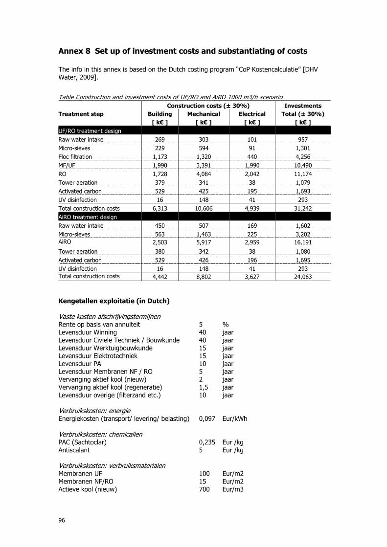
96

Annex 8 Set up of investment costs and substantiating of costs

The info in this annex is based on the Dutch costing program “CoP Kostencalculatie” [DHV Water, 2009].

Table Construction and investment costs of UF/RO and AiRO 1000 m3/h scenario

Construction costs (± 30%) Investments

Treatment step Building Mechanical Electrical Total (± 30%)

[ k€ ] [ k€ ] [ k€ ] [ k€ ]

UF/RO treatment design

Raw water intake 269 303 101 957

Micro-sieves 229 594 91 1,301

Floc filtration 1,173 1,320 440 4,256

MF/UF 1,990 3,391 1,990 10,490

RO 1,728 4,084 2,042 11,174

Tower aeration 379 341 38 1,079

Activated carbon 529 425 195 1,693

UV disinfection 16 148 41 293

Total construction costs 6,313 10,606 4,939 31,242

AiRO treatment design Raw water intake 450 507 169 1,602

Micro-sieves 563 1,463 225 3,202

AiRO 2,503 5,917 2,959 16,191

Tower aeration 380 342 38 1,080

Activated carbon 529 426 196 1,695

UV disinfection 16 148 41 293

Total construction costs 4,442 8,802 3,627 24,063

Kengetallen exploitatie (in Dutch) Vaste kosten afschrijvingstermijnen Rente op basis van annuiteit 5 % Levensduur Winning 40 jaar Levensduur Civiele Techniek / Bouwkunde 40 jaar Levensduur Werktuigbouwkunde 15 jaar Levensduur Elektrotechniek 15 jaar Levensduur PA 10 jaar Levensduur Membranen NF / RO 5 jaar Vervanging aktief kool (nieuw) 2 jaar Vervanging aktief kool (regeneratie) 1,5 jaar Levensduur overige (filterzand etc.) 10 jaar Verbruikskosten: energie Energiekosten (transport/ levering/ belasting) 0,097 Eur/kWh Verbruikskosten: chemicalien PAC (Sachtoclar) 0,235 Eur /kg Antiscalant 5 Eur /kg Verbruikskosten: verbruiksmaterialen Membranen UF 100 Eur/m2 Membranen NF/RO 15 Eur/m2 Actieve kool (nieuw) 700 Eur/m3

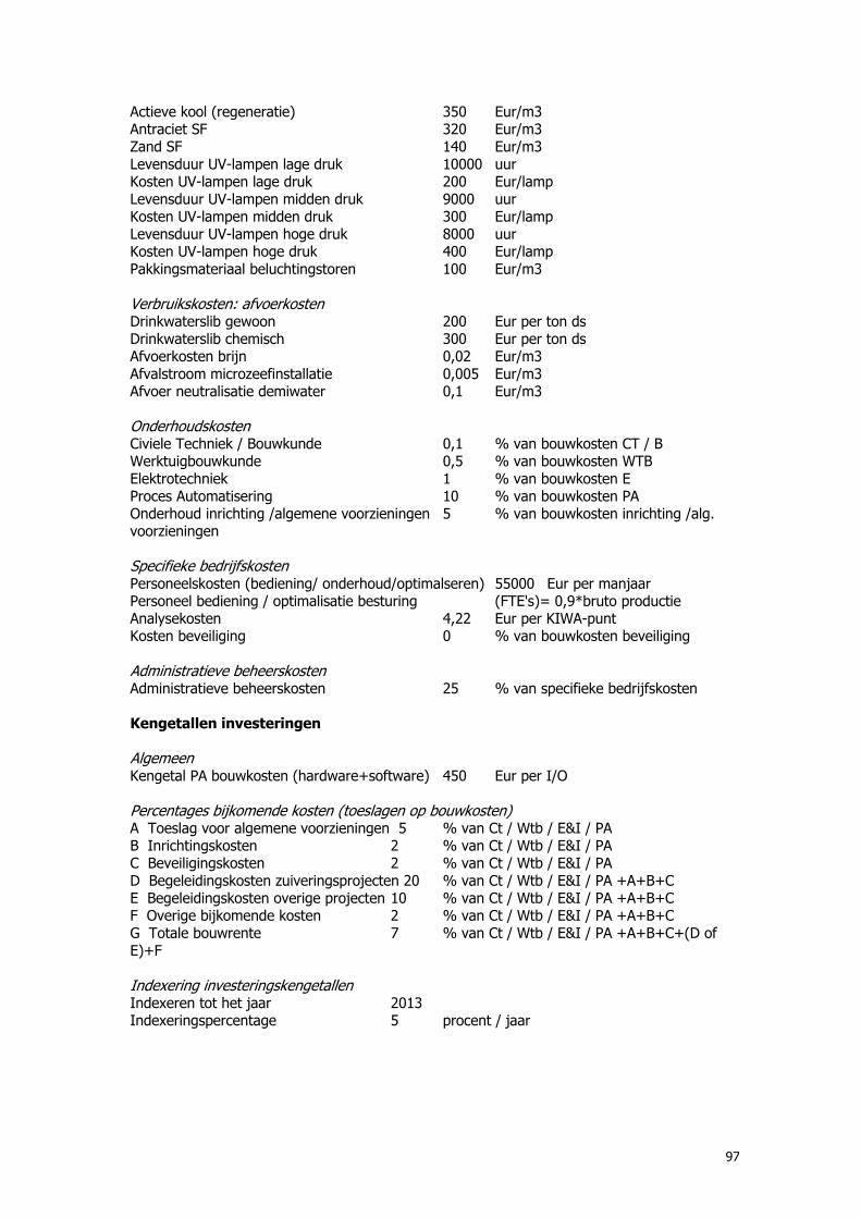
97

Actieve kool (regeneratie) 350 Eur/m3 Antraciet SF 320 Eur/m3 Zand SF 140 Eur/m3 Levensduur UV-lampen lage druk 10000 uur Kosten UV-lampen lage druk 200 Eur/lamp Levensduur UV-lampen midden druk 9000 uur Kosten UV-lampen midden druk 300 Eur/lamp Levensduur UV-lampen hoge druk 8000 uur Kosten UV-lampen hoge druk 400 Eur/lamp Pakkingsmateriaal beluchtingstoren 100 Eur/m3 Verbruikskosten: afvoerkosten Drinkwaterslib gewoon 200 Eur per ton ds Drinkwaterslib chemisch 300 Eur per ton ds Afvoerkosten brijn 0,02 Eur/m3 Afvalstroom microzeefinstallatie 0,005 Eur/m3 Afvoer neutralisatie demiwater 0,1 Eur/m3 Onderhoudskosten Civiele Techniek / Bouwkunde 0,1 % van bouwkosten CT / B Werktuigbouwkunde 0,5 % van bouwkosten WTB Elektrotechniek 1 % van bouwkosten E Proces Automatisering 10 % van bouwkosten PA Onderhoud inrichting /algemene voorzieningen 5 % van bouwkosten inrichting /alg. voorzieningen Specifieke bedrijfskosten Personeelskosten (bediening/ onderhoud/optimalseren) 55000 Eur per manjaar Personeel bediening / optimalisatie besturing (FTE's)= 0,9*bruto productie Analysekosten 4,22 Eur per KIWA-punt Kosten beveiliging 0 % van bouwkosten beveiliging Administratieve beheerskosten Administratieve beheerskosten 25 % van specifieke bedrijfskosten Kengetallen investeringen Algemeen Kengetal PA bouwkosten (hardware+software) 450 Eur per I/O Percentages bijkomende kosten (toeslagen op bouwkosten) A Toeslag voor algemene voorzieningen 5 % van Ct / Wtb / E&I / PA B Inrichtingskosten 2 % van Ct / Wtb / E&I / PA C Beveiligingskosten 2 % van Ct / Wtb / E&I / PA D Begeleidingskosten zuiveringsprojecten 20 % van Ct / Wtb / E&I / PA +A+B+C E Begeleidingskosten overige projecten 10 % van Ct / Wtb / E&I / PA +A+B+C F Overige bijkomende kosten 2 % van Ct / Wtb / E&I / PA +A+B+C G Totale bouwrente 7 % van Ct / Wtb / E&I / PA +A+B+C+(D of E)+F Indexering investeringskengetallen Indexeren tot het jaar 2013 Indexeringspercentage 5 procent / jaar

98

CV of the author Publications Ron C.M. Jong, Janneke Duiven, G. Gea Terhorst, Koos J. Baas (2013) Implementation research of new phosphorus free antiscalant at an aerobic ground water RO plant Desalination and Water Treatment 18 April 2013 Ron Jong, Anushka Salmin en Dik Brummel (2011) Grondwater zuivering in Suriname Neerslag VI, 2011 Ron C.M. Jong, Janneke Duiven, Gea Terhorst en Koos J. Baas (2011) Implementatie onderzoek naar fosfaatvrije antiscalant H2O 19 Ron C.M. Jong, Janneke Duiven, and Koos J. Baas (2011) CMI in Membrane Technology: A New Green Antiscalant International Desalination Association Journal Third Quarter 2011 Ron C. M Jong; Marc Kalf; Walter van der Meer (2010) Optiflux® RO design scoop with centre port pressure vessels for water treatment plant Dinxperlo, The Netherlands Water Practice & Technology, Vol 5 No 1 © IWA Publishing 2010 Jong, R.C.M. (08-2009) Innovatie bij Vitens In: Neerslag V 2009 Jong, R.C.M. (04-2009) Drinkwater zuivering bij Vitens In: Neerslag II 2009 Jong, R.C.M. (2007). Voordelen van een RO stack ontwerp met centre port drukvaten In: NPT Procestechniek Jong, R.C.M. (2006). Nieuw type antiscalant voor membraanfiltratie Dinxperlo In: H2O Jong, R.C.M. (2006). Ervaringen bij Vitens met lozing van membraanconcentraat In: H2O Jong, R.C.M. (2003). Hergebruik van regeneratiezout bij ionenwisseling In: H2O Jong, R.C.M. (1999). Actualisering zuiveringsopzet van Project Infiltratie Maaskant In: H2O Jong, R.C.M. (1997). Beheersing van een denitrificerende ethanol vastbed bioreactor In: H2O AiRO orientated presentations R.C.M. Jong, J.A. De Ruijter, J.Q.J.C. Verberk, W.G.J. Van de Meer (2013) AiRO; Direct Reverse Osmosis on surface water presentation at 10. Aachener Tagung Wasser und membranen 29. und 30. Oktober 2013 im Eurogress, Aachen R.C.M. Jong, J.A. De Ruijter, J.Q.J.C. Verberk, W.G.J. Van de Meer (2013) AiRO; direct Reverse Osmosis on surface water poster op 10th IWA Leading Edge Conference on Water Technologies Bordeaux R.C.M. Jong, J.A. De Ruijter, J.Q.J.C. Verberk, W.G.J. Van de Meer (2012) AiRO: Reverse osmosis on surface water without extensive pretreatment poster op Euromembrane Conference 2012 Londen Ron C.M. Jong, Jan Arie de Ruijter, Sjack van Agtmaal, Emile Cornelissen (2011) Towards reverse osmosis on surface water without extensive pretreatment: Assessment of the AiRO concept presentatie op 6th IWA Specialist Conference on Membrane Technology, Aachen October 2011

99

Ron C.M. Jong, Wilbert van de Ven, Heidi Hyppönen, Erik van der Pol, Emile Cornelissen, Jan Arie de Ruijter, Sjack van Agtmaal (2010) Towards reverse osmosis on surface water without extensive pretreatment: Initial assessment of the AiRO concept LET Phoenix, April 2010 (poster presentation).

100