airline fuel efficiency: assessment methodologies...

To appear as a book chapter in Advances in Airline Economics, edited by Peoples, J. and Bitzan,

J., Emerald Group Publishing, 2016.

1

Airline Fuel Efficiency: Assessment Methodologies and

Applications in the U.S. Domestic Airline Industry

Bo Zou1, Irene Kwan2, Mark Hansen3, Dan Rutherford2, Nabin Kafle1

1 University of Illinois, Chicago, IL, United States 2 International Council on Clean Transportation, San Francisco, CA, United States

3 University of California, Berkeley, CA, United States

Abstract Air carriers and aircraft manufacturers are investing in technologies and strategies to reduce fuel

consumption and associated emissions. This chapter reviews related issues to assess airline fuel

efficiency and offers various empirical evidences from our recent work that focuses on the U.S.

domestic passenger air transportation system. We begin with a general presentation of four methods

(ratio-based, deterministic frontier, stochastic frontier, and data envelopment analysis) and three

perspectives for assessing airline fuel efficiencies, the latter covering consideration of only

mainline carrier operations, mainline-subsidiary relations, and airline routing circuity. Airline fuel

efficiency results in the short run, in particular the correlations of the results from using different

methods and considering different perspectives, are discussed. For the long-term efficiency, we

present the development of a stochastic frontier model to investigate individual airline fuel

efficiency and system overall evolution between 1990 and 2012. Insight about the association of

fuel efficiency with market entry, exit, and airline mergers are also obtained.

1 Introduction Fuel is a major cost component in the airline industry. In mid-2015, the time of this writing, it

accounted for roughly one third of an airline’s operating costs in the U.S. Aviation jet fuel prices

remained relatively stable at $3.00/gallon from 2012 until the last quarter of 2014, when the fuel

price plunged to $1.50/gallon, mitigating the financial strain that persisted in the airline industry

over the past several years (EIA, 2015a). However, the low fuel price is not expected to persist. For

example, the U.S. Energy Information Administration predicts that jet fuel price will increase from

$1.79/gallon in 2015 to $2.23/gallon in 2016 (EIA, 2015b).

Aircraft fuel is closely related to emissions of CO2 and other gases that cause climate change (Zou

et al., 2013; Soler et al., 2014), and the airline industry has been under growing pressure to cut its

climate change impact. If counted as a country, global aviation would have ranked seventh in terms

of CO2 emissions in 2011, just after Germany and well above Korea. Moreover, global aviation

CO2 emissions are projected to triple by 2050 under business-as-usual scenarios (Kwan and

Rutherford, 2014). U.S. domestic and international flights account for about 35% of global

commercial aviation-induced CO2 emissions (Environmental Protection Agency, 2008). The U.S.

Federal Aviation Administration (FAA) forecasts that fuel consumption for the U.S. will increase

at an average rate of 2% per year over the next 20 years, increasing from 18.3 billion gallons (179

million metric tons (MMT) of CO2) in 2014 to about 26.2 billion gallons (257 MMT CO2) by 2034

(FAA, 2014).



2

Given the substantial fuel cost and climate change impact concerns, airlines have the natural

tendency to increase their fuel efficiency by, for example, adopting newer aircraft and adjusting

network structure and operational characteristics. There is considerable literature concerning the

fuel savings potential of such measures. However, this is a scant body of the literature on how

efficiently fuel is being used by airlines at a particular point in time. Building upon our recent series

of published and unpublished research on this subject, the primary objective of this chapter is

present a systematic methodological framework of airline efficiency evaluation as well as up-to-

date empirical evidence. To be more specific, this chapter discusses different methods for assessing

fuel efficiency. We consider how airline fuel efficiency is affected by mainline carriers

subcontracting service to regional affiliates, as well as the impact of routing circuity due to the hub-

and-spoke network structure. The similarities and differences between results based on different

evaluation methods are also analyzed, as are the short-term dynamics and long-term trend of airline

fuel efficiency. Finally, we examine the association of fuel efficiency with market entry, exit, and

airline mergers. The focus is on the U.S. domestic system, where most comprehensive data are

available, allowing for investigation of all the aforementioned issues. We hope that by providing

such a comprehensive coverage of the methods for assessing airline fuel efficiency and the results

of their application, this chapter will provide researchers and practitioners with a useful frame of

reference for future investigation of airline fuel efficiency and its implications for policy and

regulation.

Section 2 presents four methodologies for examining airline fuel efficiency. This is followed by a

discussion of quantifying fuel efficiency from three perspectives (i.e., considering mainline carriers

only, mainline carriers with regional affiliates, and routing circuity), in Subsection 3.1. Some

results from employing different methodologies and considering different perspectives are given in

Subsection 3.2, ensued by an illustration of the short-term airline fuel efficiency dynamics in the

U.S. domestic system. Section 4 focuses on the long-term fuel efficiency of U.S. carriers, based on

stochastic frontier modeling. The association of airline fuel efficiency with market entry, exit, and

airline consolidation is further explored in Section 5. Finally, Section 6 concludes this chapter.

2 Methodologies for measuring fuel efficiency Generally speaking, the term fuel efficiency for an airline refers to the comparison between the

observed and least possible amount of fuel consumed in producing a given level of output. Because

of the complexity of airline operations, fuel efficiency hinges upon a variety of factors including

aircraft size, market characteristics (e.g., long-haul vs. short-haul), service network structure (e.g.,

hub-and-spoke vs. point-to-point), etc. Four methods exist to assess airline fuel efficiencies. These

methods reflect different views of the airline production process. The first method is ratio-based,

which is similar to the “fuel economy” (miles per gallon) concept used to evaluate vehicle fuel

efficiency. The other three methods, namely the deterministic frontier, stochastic frontier, and data

envelopment analysis approaches, capture the multi-dimensional nature of output that airlines

produce. This section briefly reviews the concepts underlying the different methods and how they

may be applied to assess airline fuel efficiency.

2.1 Ratio-based approach The ratio-based fuel efficiency metric is simple and intuitive and often used by the industry to

determine airline fuel or environmental performance. By its name, fuel efficiency is measured as

the ratio of fuel consumed to the output produced.1 Common measures of airline output include

1 More accurately, this ratio measures “fuel inefficiency,” i.e., the higher the value, the less fuel-efficient an

airline is. However, the term “fuel efficiency” refers to either a fuel to output ratio or an output to fuel ratio.



3

available seat miles (ASM) or available ton miles (ATM), revenue passenger miles (RPM) or

revenue ton miles (RTM), and the number of flight departures (dep). ASM and ATM characterize

the capacity offered by an airline; whereas RPM and RTM are measures of utilized capacity.

Compared to using RPM or RTM, a ratio that is based on ASM or ATM would reward airlines that

provide greater capacity yet fly their planes empty (the lighter the plane, the less fuel it burns), but

does not properly account for an airline’s efforts to match capacity with traveler demand. Therefore,

RPM or RTM is preferred to ASM or ATM as the output measure. Accordingly, the fuel efficiency

metrics are fuel/RPM or fuel/RTM. RPM is a standard metric of airline production output,

especially for carriers whose passenger operations dominate the overall business. For airlines

whose cargo business account for a non-trivial portion, the use of RTM is more appropriate when

a single aggregate measure encompassing both passenger and cargo operations is desired.

An alternative view of airline production is to use flight departures (dep) instead of RPM/RTM, on

the ground that flight departures are another measure of airline production output. The

corresponding fuel efficiency measure is fuel/dep. While RPM/RTM and dep are often highly

correlated, they represent different dimensions of airline production output. RPM/RTM measures

the level of mobility provided by an airline to passengers; dep represents the extent of accessibility

offered, or the ability to reach desired goods, services, and activities (Litman, 2011). This is because

each flight departure, like the stop of a bus or a train, affords an opportunity for passengers to

embark or disembark.

An obvious question arises as to which output measure should be considered as output for

measuring airline fuel efficiency. The answer depends on which dimension of output (mobility or

accessibility) is the focus of the evaluation. Without a priori preferences, a measure that covers

both mobility and accessibility dimensions of airline output is desired. To the extent that an airline

reduces fuel use by flying non-stop for long distances, thus limiting the ability of customers to

board and alight from its vehicles, only using RPM/RTM will yield a distorted measure of the

airline’s fuel efficiency (Zeinali et al., 2013). Similarly, fuel efficiency ratios only considering dep

as the output would fail to capture the mobility aspects of airline services. Two airlines with the

same departures, one connecting distant markets and the other servicing close-by cities, would be

viewed as producing the same amount of output in terms of dep. Yet it is obvious that the first

carrier burns more fuel, everything else being equal. In reality, however, there is often a high

correlation between RPM/RTM and the number of flight departures produced.

2.2 Frontier approaches Frontier approaches can be used to define a fuel efficiency metric that accounts for both mobility

and accessibility aspects of output. As implied by the name, measurement of fuel efficiency relies

on constructing a fuel consumption frontier, which defines the minimum fuel to provide a certain

amount of output, as determined by RPM/RTM and flight departures. For simplicity, in the

remaining of Section 2 we consider RPM as the airline mobility output. A general fuel consumption

model can be expressed as

itititit depRPMffuel ),( (1)

where subscript 𝑖 denotes a specific airline and 𝑡 the time period. ),( itit depRPMf specifies the fuel

consumption frontier; and it is a non-negative deviation term.2

2 In some cases, the deviation term can enter the fuel consumption model in alternative forms, such as an

exponential multiplier of the frontier, i.e., )exp(),( itititit depRPMffuel . This is seen later in Equation (2).



4

The concept of a frontier is illustrated in Figure 1, where for simplicity only one output is

considered. The solid curve represents the fuel consumption frontier, constructed based on four

observations (data points). Because the frontier is identified based upon the minimum fuel

consumption observed for a given level of output, data points below the frontier will be unrealizable.

Point C lies on the curve, denoting the corresponding observation fuel consumption behavior is

efficient. Other observations above the frontier curve (A, B, D) represent the cases in which fuel

use does not achieve the most efficient level. The extent of inefficiency for any of these points is

calculated as ),(/]),([ ititititit depRPMfdepRPMf , which equals the ratio of two ordinates: the

ordinate of the observation (actual fuel burn) and that of the intersection point of the corresponding

vertical line with the frontier (efficient fuel burn), e.g., ||BB''||/||B'B''|| for observation B.

Figure 1. Illustration of fuel consumption efficiency frontier

2.2.1 Deterministic frontier approach The deterministic frontier approach assumes that the frontier part of the fuel consumption model in

Equation (1), ),( itit depRPMf , can be deterministically characterized. Under the usual assumption

that the frontier follows a log-linear form, the fuel consumption model can be specified as:

itititit udepRPMfuel )ln()ln()ln( 210 (2)

To estimate the unknown coefficients 210 ,, , the Corrected Ordinary Least Square (COLS)

method is used, in two steps (Kumbhakar and Lovell, 2003). The first step applies OLS to obtain

estimates of the two slopes 1̂ and 2̂ , and an initial intercept 0̂ . We calculate OLS residuals it̂

for each observation. In the second step, 0̂ is shifted downwards until it becomes 0̂ , in which no

residual is negative and at least one is zero. Thus, }ˆ{minˆˆ,00 itti and the estimated

inefficiency for airline i at time t is calculated as }]ˆ{minˆexp[)ˆexp( , ittiititu .

It can be seen that the deterministic frontier approach attributes deviations of the observed fuel

consumption from the frontier solely to inefficiency in airlines’ fuel usage. From Equation (2), the

fuel use inefficiency measure )exp( itu can be alternatively expressed as21

)(.

)exp(

1

0itit

it

depRPM

fuel,



5

where)exp(

1

0is a constant across observations (Zou et al., 2014). Essentially, the deterministic

frontier can be viewed as a ratio-based approach, with the denominator being an empirically

estimated combination of mobility and accessibility outputs.

2.2.2 Stochastic frontier approach The deterministic frontier simplifies the assumptions about the factors influencing variations in

airline fuel efficiency, in that the source of fuel efficiency encapsulates all fuel burn variations not

associated with RPM and dep. The stochastic frontier accounts for the effect of random shocks due

to uncontrollable factors (e.g., weather and plain luck) and measurement error, distinguishing them

from airlines’ true variation in fuel efficiency. This is done by adding an idiosyncratic error term

(or “random noise”), itv , to Equation (2):

ititititit uvdepRPMfuel )ln()ln()ln( 210 (3)

The corresponding fuel consumption frontier is )exp()exp( 210 ititit vdepRPM

, which due to the

introduction of itv becomes stochastic.

In order to estimate the stochastic frontier model, some distributional assumptions about itv and itu

need to be made: 1) itv ’s have identically and independently normal distributions, i.e.,

),0(iid~ 2

vit Nv ; 2) itu ’s follow some non-negative identically and independent distribution, such

as the half-normal distribution; 3) itu and itv are independently distributed. The non-negativity

ensures that actual fuel consumption is always no less than the corresponding fuel consumption on

the frontier. On the other hand, identical distributions across itu ’s can be restrictive given the quite

diverse operational environments that airlines face. A more flexible approach assumes that itu ’s

are independently but not identically distributed as non-negative truncations of a general normal

distribution:

j

uitjjit zNu ),(~ 2

, (4)

where ’s and 2

u are the efficiency parameters to be estimated. z’s are environmental variables

characterizing the heterogeneity of the mean of efficiency distributions. In the airline fuel efficiency

context, the heterogeneity comes from different operational environments as reflected by the

average stage length, aircraft size, and aircraft load factor.

Overall, model parameters ’s, ’s, and 2

u can be estimated jointly using the maximum

likelihood estimation (MLE) method. Because both itu and itv are stochastic, the estimated

residuals of the model are realizations of ititit uv , rather than itu or itv alone. However, it is

possible to find the conditional expectation ]|)[exp( itituE as a point estimator of the fuel efficiency

for each observation (Battese and Coelli, 1993; Battese et al., 2000).



6

2.3 Data Envelopment Analysis approach Different from the deterministic and stochastic frontier approaches, Data Envelopment Analysis

(DEA) is a non-parametric, linear programming based method. DEA computes the ratio between

the weighted sum of multiple outputs and the weighted sum of multiple inputs. Similar to the

frontier approaches, an advantage of DEA over the ratio-based method is that DEA can

accommodate the presence of multiple outputs in efficiency measurement. The weights are

assigned such that the ratio of the observation under consideration (called Decision Making Unit,

or DMU) is maximized, subject to the constraints that DMUs using the same weights always have

ratios between 0 and 1. In evaluating the efficiency for each observation (DMU), a different set of

efficient DMUs will be identified. This is different from the deterministic and stochastic frontier

approaches. We refer readers to Cooper et al. (2007) for further details about DEA models.

The typical application of DEA to airline studies is to investigate the overall productive efficiency.

In such cases, inputs may include fuel, labor, capital, and materials, while outputs might be RPM

and dep. There can be, however, an alternative specification that is consistent with the frontier

models in Subsections 2.2.1 and 2.2.2: while keeping both outputs only fuel is considered as the

sole input. This specification is first proposed by Tofallis (1997), who argues that doing so

eliminates input slacks, thereby precluding the possibility of hiding poor/wasteful utilization of the

input resource, as is often the case in DEA models with multiple inputs. Under the assumptions of

constant and variable returns to scale (CRS and VRS), the input-oriented linear programming

formulations are shown for CRS in (5) and VRS in (6).

λ,

min

subject to 00 Xλx

0yYλ

0λ

(5)

λ,

min

subject to 00 Xλx

0yYλ

1eλ 0λ

(6)

where X and Y are inputs and outputs: X = (xj) and Y =(yj), for 𝑗=1,…,𝑛. 𝑛 is the total number of

DMUs and subscript j is used to denote observations.3 In our application xj = fuelj and yj = (RPMj,

depj). Subscript 0 denotes the DMU under evaluation. 𝐞 is a row vector with all elements being

unity. The decision variables are 𝜃 ∈ ℝ1 and 𝛌 = (λ1, … , λ𝑛)T ∈ ℝn for both the CRS (5) and VRS

(6) formulations. The only difference between (5) and (6) is that (6) has an additional constraint,

𝐞𝛌 = 1, which limits the ways in which the observations for the 𝑛 DMUs can be combined.

Therefore, the feasible region under VRS is a subset of the feasible region of the corresponding

CRS model, and the optimal value of 𝜃 in (5) is always no greater than that in (6). Note that 𝜃 is

the ratio of the weighted sum of RPM and dep over fuel consumption. We solve for 𝜃 for each

DMU. In order to be consistent with the fuel efficiency measure in the previous methods, the fuel

inefficiency scores are 1 𝜃⁄ for each DMU.

3 For simplicity we use a single subscript j instead of two subscripts i and t to denote observations.



7

3 Recent Trends in US airline fuel efficiency In this section, we present applications of the above fuel efficiency assessment methods to the U.S.

domestic operations in the recent past. We first consider mainline airlines. The operations of these

airlines account for a bulk of the system total. A unique feature in the U.S. domestic system is that

those mainline carriers also subcontract part of their services, especially on thinner routes, to

smaller, regional affiliated carriers. Such services are still branded under the corresponding major

carrier. Therefore, it may be important to account for the regional affiliates while quantifying the

overall efficiency of branded services provided by a major carrier. In addition, the hub-and-spoke

system, which is prevalent in the U.S., implies excess fuel consumption as aircraft take air travelers

to intermediate hubs before reaching their final destinations. The resulting route circuity reduces

fuel efficiency if output is measured in terms of the distances between passengers’ origins and

destinations. The effect of routing circuity on fuel efficiency will also be presented here. This

allows us to compare efficiency results that account for the use of regional carriers and indirect

routings with results when these factors are not considered. Using the deterministic frontier method

as an example, the last part of this section presents an investigation of the short-term fuel efficiency

changes since 2010.

3.1 Three perspectives on airline fuel efficiency

3.1.1 Considering mainline carriers only The first step to assess mainline carrier fuel efficiency is to identify the mainline carriers, which is

based on two criteria. The first is the size. We choose a minimum of 500,000 domestic

enplanements as the cutoff point. In 2013, 31 U.S. carriers met this threshold. The second criterion

is based on average aircraft size for domestic operations in 2013. As shown in Figure 2, there is a

clear demarcation between Jet Blue and Republic Airlines. Only those carriers on the left side,

whose fleet consists of mainly narrow- and wide-body jets, will be considered as candidates for

mainline carriers. In 2013, there were 13 airlines identified as mainline carriers satisfying both

criteria. The selected mainline carriers operate predominately passenger flights, with only a small

fraction dedicated to cargo.

Source: Data Base Products (2014)

Figure 2. Average aircraft size of U.S. carriers on passenger domestic operations in 2013

0

20

40

60

80

100

120

140

160

180

AllegiantAir

SpiritAirLines

DeltaAirLinesInc.

United

AirLinesInc.

AmericanAirlinesInc.

Haw

aiianAirlinesInc.

USAirwaysInc.

SunCountryAirlines

AlaskaAirlinesInc.

Fron

erAirlines-Inc.

SouthwestAirlinesCo.

VirginAmerica

JetBlue

Rep

ublicAirlines

HorizonAir

CompassAirlines

MesaAirlines,Inc.

Shu

leAmericaCorp.

GoJetAirlines

PinnacleAirlines

PSA

Airlines-Inc.

Skyw

estAirlinesInc.

ExpressJetAirlines(ASA

)

AmericanEagleAirlinesInc.

AirW

isconsinAirlinesCorp

TransStatesAirlines

ChautauquaAirlines,Inc.

PiedmontAirlines

Commutair

SilverAirways

CapeAir

Seats



8

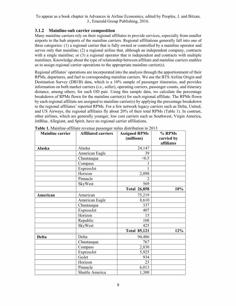
3.1.2 Mainline-sub carrier composition Many mainline carriers rely on their regional affiliates to provide services, especially from smaller

airports to the hub airports of the mainline carriers. Regional affiliations generally fall into one of

three categories: (1) a regional carrier that is fully owned or controlled by a mainline operator and

serves only that mainline; (2) a regional airline that, although an independent company, contracts

with a single mainline; or (3) a regional operator that is independent and contracts with multiple

mainlines. Knowledge about the type of relationship between affiliate and mainline carriers enables

us to assign regional carrier operations to the appropriate mainline carrier(s).

Regional affiliates’ operations are incorporated into the analysis through the apportionment of their

RPMs, departures, and fuel to corresponding mainline carriers. We use the BTS Airline Origin and

Destination Survey (DB1B) data, which is a 10% sample of passenger itineraries, and provides

information on both market carriers (i.e., seller), operating carriers, passenger counts, and itinerary

distance, among others, for each OD pair. Using this sample data, we calculate the percentage

breakdown of RPMs flown for the mainline carrier(s) for each regional affiliate. The RPMs flown

by each regional affiliate are assigned to mainline carrier(s) by applying the percentage breakdown

to the regional affiliates’ reported RPMs. For a few network legacy carriers such as Delta, United,

and US Airways, the regional affiliates fly about 20% of their total RPMs (Table 1). In contrast,

other airlines, which are generally younger, low cost carriers such as Southwest, Virgin America,

JetBlue, Allegiant, and Spirit, have no regional carrier affiliations.

Table 1. Mainline-affiliate revenue passenger miles distribution in 2013

Mainline carrier Affiliated carriers Assigned RPMs

(millions)

% RPMs

carried by

affiliates

Alaska Alaska 24,147

American Eagle 39

Chautauqua <0.5

Compass 1

ExpressJet 1

Horizon 2,098

Pinnacle 2

SkyWest 569

Total 26,858 10%

American American 75,219

American Eagle 8,610

Chautauqua 337

ExpressJet 407

Horizon 15

Republic 108

SkyWest 425

Total 85,121 12%

Delta Delta 94,486

Chautauqua 767

Compass 2,830

ExpressJet 5,925

GoJet 934

Horizon 23

Pinnacle 6,013

Shuttle America 1,300



9

SkyWest 4,760

Total 117,039 19%

Frontier Frontier 8,635

Chautauqua <0.5

Republic 297

Total 8,932 3%

Hawaiian Hawaiian 9,082

SkyWest <0.5

Total 9,082 ~0

United United 92,912

Air Wisconsin 8

Chautauqua 463

Commutair 261

ExpressJet 9,452

GoJet 1,553

Mesa 1,158

Piedmont 25

PSA 40

Republic 643

Shuttle America 2,397

SkyWest 8,057

Trans States 871

Total 117,838 21%

US Airways US Airways 49,442

Air Wisconsin 2,133

Chautauqua 107

ExpressJet 158

GoJet 41

Mesa 2,823

Piedmont 496

PSA 1,805

Republic 3,666

Shuttle America 63

SkyWest 793

Trans States 45

Total 61,573 20%

Due to the lack of relevant data, we assume the assignment of regional carrier departures and fuel

to mainline carriers to be proportional to the RPM assignment. The resulting adjusted RPM,

departures, and fuels values are then used in the various fuel efficiency assessment models.

3.1.3 Routing circuity A considerable portion of passengers make connections at an intermediate hub airport in their trips.

From the airlines’ perspective, more fuel burn will result from circuitous routes and additional

takeoffs and landings. If the focus is on fuel efficiency in terms of transporting passengers from

their true origins to true destinations, then airlines operating more direct routes should be rewarded

as opposed to those flying connecting, more circuitous itineraries. Figure 3 depicts the effects of



10

circuity on fuel burn for one-stop flights from San Francisco (SF) to New York (NY). A flight

routing through Chicago follows the great circle path, while a flight going through Atlanta or

Houston, deviates significantly from the great circle path between SF and NY and burns about 11%

and 15% more fuel per flight, respectively.

Source: Zeinali et al. (2013)

Figure 3. Example of possible routes from San Francisco to New York by distance

We introduce the following circuity measure to capture the excess amount of distance traveled from

passengers’ true origin airports to their final destination airports, as compared to the non-stop, great

circle distance (GCD) routes. For a passenger, his/her itinerary circuity is equal to 1 when the

journey is direct and greater than 1 otherwise.4 The itinerary distance and the GCD between the

origin and destination airports for each passenger are collected and aggregated over all passengers

taking a mainline airline (and its affiliate(s)), to come up with the mainline airline-specific circuity:

milespassenger GCD total

flown milesitinerary passenger totalCircuity (4)

Using the calculated airline circuity measure, a new output metric, revenue passenger OD miles

(RPODM) which incorporates the routing circuity effect, is introduced in place of RPM in the fuel

efficiency assessment:

Circuity

RPMROPDM (5)

4 Note that a flight with a layover is not necessarily circuitous. If the layover airport lies on the great circle

path of the flight (e.g., SF-Chicago-NY in Figure 3), then it will have a circuity equal to 1; otherwise circuity

is greater than 1 (e.g., SF-Atlanta-NY and SF-Houston-NY).



11

Given that two airlines have the same fuel consumption and RPMs, the airline with more circuitous

routing is then penalized by having a lower RPODM output, crediting airlines by flying passengers

more directly between passengers’ intended origins and destinations.

3.2 Correlation of various airline efficiency results With the four different frontier methods applied and the three perspectives of considering mainline-

only, mainline-regional affiliates, and routing circuity, there will be a combination of 12 (4×3)

airline fuel efficiency estimates. While having a comprehensive comparison among these estimates

is beyond the scope of this chapter, in this subsection we selectively present our previous

correlation analysis results on how the efficiency estimates are correlated. More detailed analysis

can be found in Zou et al. (2014).

Table 2 presents the pair-wise Pearson correlation and Spearman rank correlation coefficients for

the inefficiency scores obtained from applying the ratio-based, deterministic frontier, stochastic

frontier, and variable returns to scale (VRS) DEA models to the U.S. mainline carriers only in 2010.

Overall, the efficiency results from different methods are in good agreement. The highest degree

of agreement occurs between the deterministic and stochastic frontier approaches, and the ratio-

based approach seems to have least agreement with the other three methods. This is not surprising,

as the ratio-based approach only include one output (in Table 2, it is RPM), whereas both RPM and

dep are considered as outputs in the other methods. Indeed, the strong correlations among the

efficiency scores from the last three methods suggest the robustness of the fuel efficiency findings

to different methods used.

Table 2. Comparison of 2010 mainline airline fuel efficiency results using (a) Pearson correlation

coefficients and (b) Spearman ranking correlation coefficients

(a) Inefficiency Scores Correlation

Ratio-based Deterministic

frontier

Stochastic

frontier

VRS

DEA

Ratio-based 1

Deterministic frontier 0.8271 1

Stochastic frontier 0.7071 0.9818 1

VRS DEA 0.6673 0.8291 0.8169 1

(b) Spearman Inefficiency Ranking Correlation

Ratio-based Deterministic

frontier

Stochastic

frontier

VRS

DEA

Ratio-based 1

Deterministic frontier 0.8607 1

Stochastic frontier 0.5643 0.8964 1

VRS DEA 0.6857 0.8464 0.8143 1

Source: Zou et al. (2014)

For many mainline airlines, regional affiliates account for a small portion of the mainline-regional

combined operations. As a consequence, we do not expect substantial changes in fuel efficiency

when regional affiliates are taken into consideration. In addition, empirical data show that while

some mainline airlines choose hub-and-spoke operations, the itineraries are indeed judiciously

designed, resulting in small overall network routing circuity. For example, the highest routing

circuity among the mainline carriers in 2010, which occurred to US Airways, is only 1.068 (Zou et

al., 2014). This suggests that considering RPODM instead of RPM will not yield significantly



12

different efficiency results, as is confirmed by the efficiency correlation results in our previous

study (Zou et al., 2014). To further demonstrate this, Table 3 reports the airline fuel efficiency

ranking considering mainlines only, mainline-regional affiliates, and routing circuity in 2013, using

the deterministic frontier approach. It is clear that only minor ranking shifts exist across the three

cases.

Table 3. Airline fuel efficiency rankings in 2013 using the deterministic frontier method

Rank Mainline-only Mainline-affiliate With routing circuity

1 Frontier Alaska Alaska

2 Spirit Frontier Spirit

3 Alaska Spirit Frontier

4 United Southwest Southwest

5 Hawaiian Hawaiian Hawaiian

6 Southwest United United

7 Virgin Delta JetBlue

8 Delta Virgin Delta

9 JetBlue JetBlue Virgin

10 US Airways US Airways US Airways

11 Allegiant Sun Country Sun Country

12 Sun Country Allegiant Allegiant

13 American American American

3.3 Short-term dynamics of airline fuel efficiency This subsection provides a picture of the short-term airline fuel efficiency dynamics among

mainline carriers in the U.S., using the deterministic frontier model as an example. While one may

also use other methods to perform such analysis, the preceding discussions have shown a high

degree of agreement among the efficiency results from adopting different methods (especially the

frontier and DEA methods). The following ranking results in Table 4 are obtained by developing a

fuel efficiency frontier each year from 2010 to 2013. The last column shows the excess fuel burn

in 2013 for a given airline compared to the most efficient one, while producing the same amount

of outputs. The model consider both regional affiliate operations and routing circuity.

Table 4. Airline fuel efficiency rankings for U.S. domestic operations using the deterministic

frontier method (including regional affiliates and circuity), 2010–2013

Rank 2010 2011 2012 2013 Excess fuel

burn, 2013

1 Alaska Alaska Alaska Alaska* —

2 Spirit* Spirit Spirit Spirit* —

3 Hawaiian* Southwest†* Southwest* Frontier* —

4 Continental Hawaiian* Hawaiian* Southwest +4%

5 Southwest Frontier Frontier Hawaiian +9%

6 Frontier Continental‡ United United +10%

7 JetBlue JetBlue JetBlue JetBlue +13%

8 United United‡ Virgin* Delta +14%

9 Virgin Delta Delta* Virgin* +15%

10 Sun Country Sun Country* US Airways* US Airways* +15%



13

11 Delta US Airways* Sun Country Sun Country +20%

12 US Airways Virgin* Allegiant* Allegiant +21%

13 AirTran AirTran† American* American +27%

14 American American -- -- --

15 Allegiant Allegiant -- -- --

* Tie (in a given year) †Merged ‡Merged5

Source: Kwan and Rutherford (2014)

The relative efficiency of fuel use remains rather stable during the study period, despite slight

fluctuations of rankings for some airlines, mostly within a couple of places. Overall, the large,

legacy carriers (e.g., American, Delta, United) remained in the middle or lower rungs of the airline

efficiency ladder. Alaska and Spirit were the most fuel-efficient airlines; American and Allegiant

were the two least fuel-efficient airlines from 2010-2013. The fuel efficiency gap between the best

(Alaska) and worst performing (American) airline was roughly 27% in 2013, and this gap keeps

stable over the four-year period. Alaska and Spirit had very fuel-efficient fleets and efficient

operational practices (e.g., higher seating densities and load factors). In 2013, Alaska flew an

increasing percentage of its RPMs on Boeing 737-800 and 737-900 aircraft, and its regional flights

on fuel-efficient Dash 8 turboprop aircraft via its affiliate partner Horizon Air. Spirit made aircraft

improvements through the use of new A320s with Sharklets, which can reduce fuel by up to 4%.

A typical Spirit A320 aircraft carried up to 36 more people on a flight than on a similar aircraft

flow by its rivals, and flew 34% more passenger miles per pound of fuel. Both Alaska and Spirit

had relatively young fleets and flew with passenger load factors averaging over 85%. All these

contributed to the top fuel efficiency of the two airlines.

Frontier leapfrogged Southwest and Hawaiian to tie for first with a 10% fuel efficiency

improvement from 2012 to 2013. In 2012, Indigo Partners, a private equity and venture capital firm,

purchased Frontier and has been transforming the airline into an ultra-low-cost carrier, leading to

significant changes in its fare structure and flight operations. Frontier reduced its total flights by

about 33% as well as its regional affiliate operations from 14% of its total RPMs in 2012 to only

3% in 2013. Moreover, Frontier’s load factor improved to 91%, the highest on U.S. domestic

operations, thereby transporting more passengers on an average flight. Since 2011, it also began to

phase out its less efficient Airbus A318 aircraft, for larger A319 and A320 aircraft.

On the other end of the fuel efficiency spectrum, Allegiant and American tied in 2012 for having

the least-efficient U.S. domestic operations. Since then Allegiant has made significant

improvements, while American’s fuel efficiency continues to stagnate. Though still flying a

majority of its flights on older MD-80 aircraft, Allegiant has been adding second-hand Boeing 757-

200, Airbus A320 and A319 aircraft to its fleet starting from 2011, for higher capacity and longer

range. The average flight flown by Allegiant in 2013 was 7% larger (12 more seats on average)

with a 6% higher seating density than in 2012. For American, although it has been flying a greater

proportion of its RPMs on Boeing 737-800’s rather than on older MD-80 aircraft, it still has the

third oldest fleet (after Allegiant and Delta).

Other notable airlines include Hawaiian, whose relative fuel efficiency has slipped in recent years

as other airlines continue to improve. In 2013, Hawaiian made changes to its flight operations

including flying almost 50% of its RPMs on newer A330-200 aircraft (introduced in 2010) and 42%

on older Boeing 767-300ER aircraft, as compared to 37% on A330-200 and 54% on B767-300ER

aircraft in 2012. However, the greater use of A330-200 aircraft does not seem to be sufficient in

5 Although both pairs of airlines (United and Continental, Southwest and AirTran) merged in 2010, their fuel

and operations data are reported jointly to BTS beginning in 2012.



14

improving the airline’s overall fuel efficiency. Southwest shifted down to the fourth as Frontier

moved up to the third in 2013, although Southwest continued to make some efficiency

improvements even after its merger with much less efficient AirTran Airways in 2012.

4 Long-term US airline fuel efficiency trend, 1991-2012 So far our discussions on airline fuel efficiency have been focused on the recent past. For policy

making purposes, it is of equivalent or even more interest to assess the fuel consumption behavior

over a longer time horizon. Taking advantage of a publically available dataset documenting airline

operations and fuel consumption, this section demonstrates the development of stochastic frontier

models to quantify the evolution of fuel efficiency among a larger, more inclusive set of airlines in

the U.S. domestic system over the past two decades.

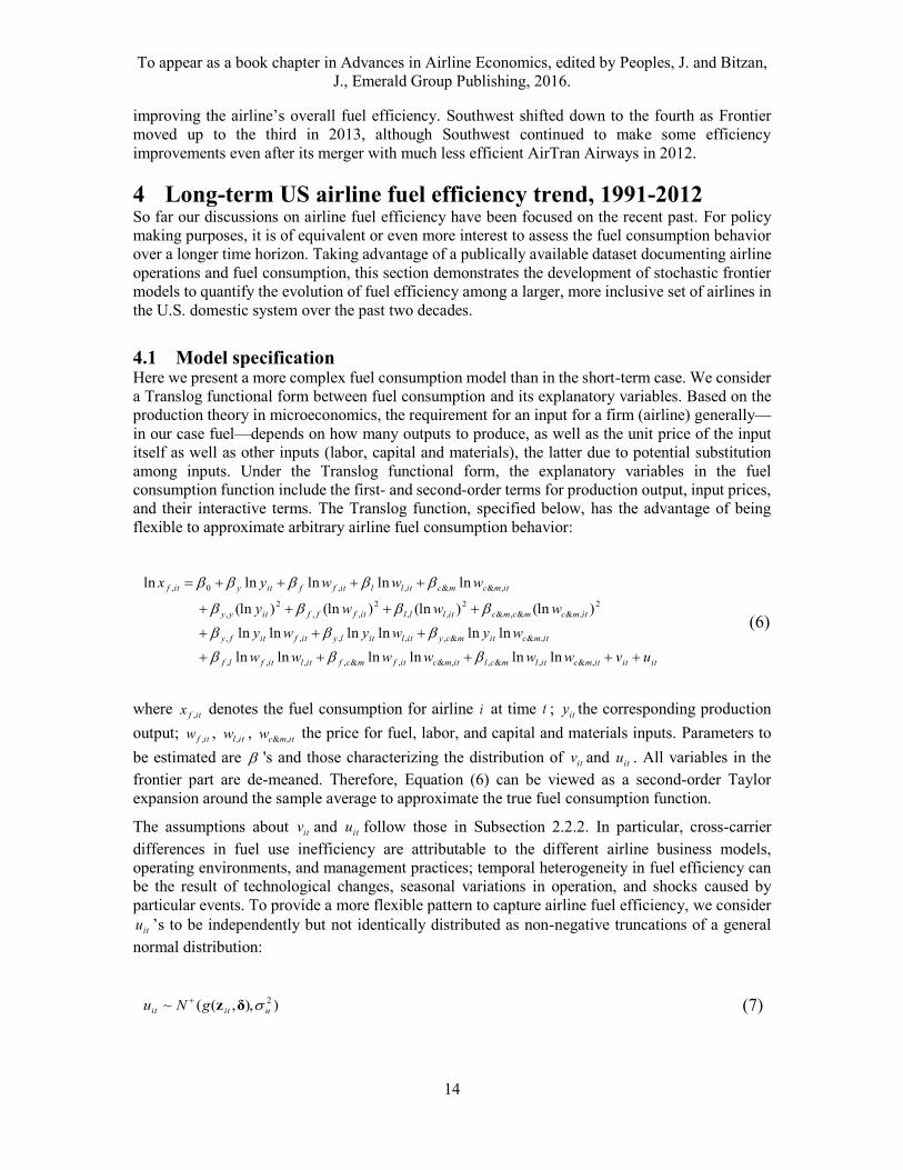
4.1 Model specification Here we present a more complex fuel consumption model than in the short-term case. We consider

a Translog functional form between fuel consumption and its explanatory variables. Based on the

production theory in microeconomics, the requirement for an input for a firm (airline) generally—

in our case fuel—depends on how many outputs to produce, as well as the unit price of the input

itself as well as other inputs (labor, capital and materials), the latter due to potential substitution

among inputs. Under the Translog functional form, the explanatory variables in the fuel

consumption function include the first- and second-order terms for production output, input prices,

and their interactive terms. The Translog function, specified below, has the advantage of being

flexible to approximate arbitrary airline fuel consumption behavior:

itititmcitlmclitmcitfmcfitlitflf

itmcitmcyitlitlyitfitfy

itmcmcmcitlllitfffityy

itmcmcitllitffityitf

uvwwwwww

wywywy

wwwy

wwwyx

,&,&,,&,&,,,,

,&&,,,,,

2

,&&,&

2

,,

2

,,

2

,

,&&,,0,

lnlnlnlnlnln

lnlnlnlnlnln

)(ln)(ln)(ln)(ln

lnlnlnlnln

(6)

where itfx , denotes the fuel consumption for airline i at time t ; ity the corresponding production

output; itfw , , itlw , , itmcw ,& the price for fuel, labor, and capital and materials inputs. Parameters to

be estimated are 's and those characterizing the distribution of itv and itu . All variables in the

frontier part are de-meaned. Therefore, Equation (6) can be viewed as a second-order Taylor

expansion around the sample average to approximate the true fuel consumption function.

The assumptions about itv and itu follow those in Subsection 2.2.2. In particular, cross-carrier

differences in fuel use inefficiency are attributable to the different airline business models,

operating environments, and management practices; temporal heterogeneity in fuel efficiency can

be the result of technological changes, seasonal variations in operation, and shocks caused by

particular events. To provide a more flexible pattern to capture airline fuel efficiency, we consider

itu ’s to be independently but not identically distributed as non-negative truncations of a general

normal distribution:

)),,((~ 2

uitit gNu δz (7)



15

Similar to before, itz is a vector of airline operational characteristics and time-related variables; δ

and 2

u are the parameters to be estimated. It is clear that the mean of the efficiency distribution

will have an influence on the "distance" between an airline's actual fuel consumption and the best

practice frontier. Here we include in z the average load factor ( LF ), average stage length ( SL ),

average aircraft size ( GAUGE ), and two dummy variables denoting whether the observation

appears after the 9/11 terrorism attack ( 911After ), and whether an airline belongs to the legacy

carrier group ( Legacy ). In addition, a time trend variable t (1 for the first period, 2 for the second

period, etc.) is introduced to capture the effect of aircraft technology and air traffic operation

improvement over time on fuel efficiency. We further add three seasonal dummies ( 3,2,1 qqq ) to

test the strength of seasonal variations in airline fuel efficiency. Compared to Subsection 2.2.2, a

richer set of variables are considered to capture long-term efficiency variations. Taking all

continuous variables in logarithmic form, ),( δzitg can be written out as:

321

911lnlnln),(

321

9110

qqqtLegacy

AfterGAUGESLLFg

qqqtLegacy

AfteritGAUGEitSLitLFit

δz (8)

Again, parameters in Equation (6) and (8) will be jointly estimated using the MLE method. With

the estimated parameters we calculate the residuals it

which are the realizations of ititit uv ,,

and then use conditional expectation ]|)[exp( itituE

as a point estimator of the fuel efficiency for

each observation.

4.2 Data As before, we focus on domestic operations of large US jet operators whose average aircraft size

is above 100 seats. Since the objective is to investigate the long-term fuel efficiency of airlines,

including as many years as possible is desired. We consider a period of over two decades—from

the first quarter of 1991 to the third quarter of 2012—the maximum time span during which we

could access relevant airline information (by airline-quarter) from the US Bureau of Transportation

Statistics (BTS) Online Data Library when this study was conducted.

Besides fuel consumption, here we consider RTM to represent production output in the long-term

stochastic frontier model. The two primary reasons for only having RTM as output are: 1) model

simplicity, since the Translog specification with RTM already implies many terms and coefficients

to be estimated; and 2) high correlation between RTM and dep in the dataset (correlation coefficient

0.84). Nonetheless, we could alternatively include both RTM and dep as outputs. The prices of the

three inputs are calculated as follows. Fuel and labor prices are calculated using fuel expenses per

gallon and labor expense per full time equivalent employee for each quarter. We follow the spirit

of Goh and Young (2006) and Merkert and Hensher (2011) and use total Available Ton Miles

(ATM) as a proxy for capital. Capital expenses consist of rental, depreciation, and amortization

costs. Materials cost is the catch-all cost (Oum and Yu, 1998), and includes expenses related to the

purchase of materials and services, landing fees, and all other remaining cost items. Capital-

materials price is then the sum of capital and materials costs divided by ATM. We consider

American, Alaska, Continental, Delta, Hawaiian, Northwest, United, and US Airways as legacy

carriers, and the post-911 period as starting from the fourth quarter of 2001.

The dataset is an unbalanced panel as the period of interest witnessed a number of airline exits,

acquisitions, and mergers. In addition, some carriers with small sizes do not regularly report their

full operational and financial data to BTS. To mitigate the potential issue of erroneous data



16

reporting, airlines with fewer than four complete observations are removed from the dataset. The

final dataset for subsequent model estimation contains 907 airline-quarter observations. Table 5

lists the airlines, their types, status, and the corresponding time periods included in our dataset. The

reported airline-quarter pairs account for the bulk of RTM services provided in the US domestic

air transportation system—over 80% in most periods. Understanding fuel efficiency of these

airlines, therefore, will provide a fairly good picture of the overall fuel consumption behavior in

the entire system.

Because of the long-term nature of the analysis, the available data do not allow for tracking the

airline-regional affiliate relationships or the routing circuity of airlines over the entire horizon.

Therefore, the subsequent analysis deals with mainline only case.

Table 5. Airline-quarter pairs included in the final dataset

Carrier Name Type Data* Remarks

AirTran Non-legacy

1997Q1-1997Q3,

2010Q4,

2011Q1- 2012Q4

Merged with Southwest in 2010

Alaska Legacy 1991Q1-2012Q3 In service

America West Non-legacy 1992Q1-2007Q3 Merged with US Airways in 2005

American Legacy 1991Q1-2012Q3 In service

Carnival Non Legacy 1992Q1-1998Q1 Ceased operations in 1998

Continental Legacy 1991Q1-2011Q4 Merged with United in 2010

Delta Legacy 1991Q1-2012Q3 In service

Frontier Non Legacy 2009Q4-2012Q3 In service

Hawaiian Legacy 1991Q1-2012Q3 In service

JetBlue Non-legacy 2002Q4-2012Q3 In service

Kiwi

International Non-legacy

1992Q4-1993Q1,

1994Q1-1994Q2,

1998 Q3-1998Q4

Ceased operations in 1999

Midwest Non-legacy 2003Q3-2008Q3 Merged with Republic Airways

Holdings in 2009

Northwest Legacy 1991Q1-2009Q4 Merged with Delta in 2008

Southwest Non-legacy 1991Q1-2012Q3 In service

Spirit Non-legacy 2010Q4-2012Q3 In service

Sun Country Non-legacy 2011Q3-2012Q3 In service

US Airways Legacy 1997Q1-2012Q3 In service

USA 3000 Non-legacy 2010Q4-2011Q4 Ceased operations in 2012

United Legacy 1991Q1-2012Q3 In service

Virgin America Non Legacy 2010Q4-2012Q3 In service * The following airline-quarter observations are incomplete: Alaska: 2001Q1, 2006Q2-Q4, 2007Q1-2010Q3; America

West: 2002Q3; American: 1992Q3; Carnival: 1993Q1, 1997Q3; Hawaiian: 1992-1994, 1995Q3, 1999Q4, 2001Q1,

2002Q3; Midwest: 1999Q3; Southwest: 1997Q1, 1998Q1; Sun Country: 2011Q3; US Airways: 1997Q4, 1998Q2.

4.3 Model estimation results The MLE results for Equations (6) and (8) are displayed under Model 1 in Table 6. For the frontier,

most of the first-order coefficients, which indicate the sensitivity of fuel input demand to various

regressors at the sample mean, are significant and have expected signs. The coefficient for RTM is

0.98—almost equal to one, suggesting that fuel demand is proportional to output. This result is



17

consistent with the constant returns-to-scale (RTS) findings in the airline cost modeling literature

(e.g., Gillen et al., 1990; Hansen et al., 2001; Zou and Hansen, 2012). The first-order coefficients

for inputs prices represent the own and cross elasticities of fuel demand, at the sample average. The

own price elasticity is about -0.05, which suggests that a 10 percent increase in fuel price would

cause fuel demand to drop by 0.5 percent. The coefficient for labor price is positive but insignificant,

which reflects the limited possibilities for substitution between the two inputs. As pointed out by

Banker and Johnston (1993), once managerial choices—which include those pertaining to aircraft,

network configuration, hub concentration, and flight frequency—have been made, opportunities

for direct substitution between labor and fuel is very limited. On the contrary, we observe a positive,

highly significant coefficient for the capital-materials price variable, which corroborates the

conventional wisdom on the substitution possibilities between fuel and capital-materials. For

example, an airline might be more inclined to preserve its older fleet if purchasing/leasing new

aircraft becomes more expensive. The coefficient implies that, if capital-materials price was

increased by 10%, fuel demand would rise by 0.8% at the sample average.

Table 6. Main model estimation results

Variable Model 1 Model 2

Est. Std. Err. Est. Std. Err.

Frontier coefficients

ln(RTM) 0.979*** 0.003 0.979*** 0.003

ln(Fuel price) -0.052*** 0.009 -0.052*** 0.009

ln(Labor price) 0.005 0.016 0.006 0.016

ln(Capital-materials price) 0.086*** 0.012 0.086*** 0.012

[ln(RTM)]2 0.053*** 0.004 0.053*** 0.004

[ln(Fuel price)]2 -0.014 0.018 -0.012 0.018

[ln(Labor price)]2 -0.148*** 0.024 -0.148*** 0.024

[ln(Capital-materials price)]2 0.034** 0.017 0.034** 0.017

ln(RTM)*ln(Fuel price) 0.036*** 0.004 0.035*** 0.004

ln(RTM)*ln(Labor price) -0.029*** 0.010 -0.029*** 0.010

ln(RTM)*ln(Capital-materials price) -0.085*** 0.010 -0.084*** 0.010

ln(Fuel price)*ln(Labor price) -0.015 0.021 -0.015 0.021

ln(Fuel price)*

ln(Capital-materials price) -0.071*** 0.015 -0.071*** 0.015

ln(Labor price)*

ln(Capital-materials price) 0.246*** 0.025 0.245*** 0.025

Constant -0.430 9.192 -0.449 8.288

Efficiency coefficients

ln(Load factor) -0.812*** 0.044 -0.802*** 0.037

ln(Stage length) -0.163*** 0.010 -0.163*** 0.010

ln(Gauge) -0.381*** 0.020 -0.384*** 0.020

Legacy dummy 0.055*** 0.008 0.055*** 0.008

After911 dummy -0.043*** 0.010 -0.043*** 0.010

Time trend -0.0007** 0.0003 -0.0007** 0.0003

Q1 (dummy) 0.006 0.006

Q2 (dummy) 0.003 0.007

Q3 (dummy) 0.008 0.007



18

Constant 3.132 9.193 3.171 8.289

2

u 0.0001 0.0354 0.0002 0.0453

2

v 0.0040 0.0354 0.0039 0.0453

RTS 1.021 0.003 1.021 0.003

Log likelihood 1210.24 1209.34

Number of observations 907 907

*** Significant at 1% level; ** Significant at 5% level; * Significant at 10% level.

Several second order coefficients which are statistically significant on the frontier part are also

worth noticing. The positive coefficient for [ln(RTM)]2 suggests that, as the output of an airline's

operation increases, fuel demand becomes more sensitive to the output. This may be due to the fact

that larger operation scales often correlate with more complex service networks and operations,

which are likely to result in additional fuel burn. In addition, we observe a negative coefficient for

the interaction term between fuel and capital-materials prices. This implies that, ceteris paribus,

airlines' demand for fuel seems more sensitive to fuel price when they face a higher capital-

materials price. Finally, with both labor and capital-materials being substitutes for the fuel input,

an airline would be, understandably, more inclined to substitute capital-materials for fuel if labor

becomes more expensive (and vice versa), as is evidenced by the positive sign of the ln(Labor

price)*ln(Capital-materials price) coefficient.

Turning now to the efficiency coefficients, we observe that all three operating environment

variables, load factor, stage length, and gauge, have negative, highly significant coefficients. Before

delving into the specific coefficients, it is important to recall RPM = (Flight departures) * (Stage

length) * (Gauge) * (Load factor), which denotes an intrinsic relationship in the airline production

process. While we use RTM instead of RPM in estimating the model, the airlines considered in the

present study are all passenger service focused, so the two variables are virtually collinear.

Consequently, when we use RTM instead of RPM the above relationship should still hold so long

as we add the appropriate multiplier. Holding RTM, stage length, and gauge constant, an increase

in load factor is associated with a reduction in flight departures, which are perceived as more fuel

demanding because of the takeoff/landing cycles involved. Higher load factor also means flying

fuller planes, which make operations more fuel efficient in producing the same amount of RTMs.

Both aspects contribute to the negative sign for the load factor coefficient. Economies of stage

length and aircraft size have been widely recognized in aircraft economics (Wei and Hansen, 2003;

Givoni and Rietveld, 2009; Ryerson and Hansen, 2013), which, together with concurrent reduction

in flight departures, explain the negative signs for the stage length and gauge coefficients. The

negative signs for the stage length and gauge coefficient are, in a broad sense, consistent with the

findings in Coelli et al. (1999), who argue that firms with low density networks (i.e. larger aircraft

size and longer stage length) benefit from a more favorable environment and therefore performs

better. In terms of the magnitude, it is not surprising that efficiency is mostly sensitive to load factor,

which directly affects aircraft payload. The larger coefficient (in absolute value) for gauge as

compared to stage length may further suggest greater economies of aircraft size than economies of

stage length.6

The efficiency estimates also reveal that legacy carriers tend to be less fuel efficient than their non-

legacy counterparts, perhaps because of production processes that were developed in an era of

lower fuel prices. It also appears that fuel efficiency increases after the 9/11 terrorism attack. This

led to a substantial decline in air travel demand and has also hastened the reorganization of the US

airline industry. Many airlines, which either had long-standing financial issues before 9/11 or over-

6 Similar implications are also found in Ryerson and Hansen (2013) from the aircraft operating cost

perspective.



19

expanded during the better economic climate of the 1990s, were forced to tighten their belts,

grounding planes, and even filing for bankruptcy (Logan, 2013). The aircraft they ceased operating

would be older, less fuel efficient ones. The result of this restructuring appears to be improved fuel

efficiency. The time trend coefficient clearly indicates that fuel efficiency continues to improve

over time due to technological advances, including improvement in engine efficiency, airframe

materials and design, and air traffic management. However, it is difficult to discern the exact extent

using the coefficient estimates because the time trend variable enters the mean of an inefficiency

term, which follows a truncated normal distribution. More quantitative evaluation of the efficiency

improvement over time will be deferred to Subsection 4.4. Seasonal variation does not seem to

affect efficiency, as all three quarterly dummy coefficients turn out insignificant. A likelihood ratio

also fails to reject the null hypothesis that 0321 qqq . We therefore re-estimate the frontier

model without the seasonal dummies. The estimation results for the other terms, as shown in Table

6 under Model 2, remain largely invariant.

4.4 Fuel efficiency assessment With the frontier model estimates, we now choose Model 2 and compute the conditional

expectation ]|)[exp( itituE

. Figures 4 and 5 depict the yearly average fuel efficiency scores (i.e.,

]|)[exp( itituE

) for legacy and non-legacy carriers respectively. Both graphs demonstrate an

improving trend, despite short-term fluctuations. The best efficiency score (1.063) occurred for

Hawaiian in the third quarter of 2005.

Within the legacy carrier group, Hawaiian remains the most efficient airline almost over the entire

time span, due to having the highest load factor (quarterly average 0.823) and largest aircraft size

(quarterly average 242 seats) among legacy carriers. By contrast, Alaska was significantly less

efficient than its peers, especially during the early 1990s, which may be attributed to its relatively

low load factor (quarterly average 0.68) and small aircraft size (quarterly average 133 seats), in

addition to its large, fuel inefficient Boeing 727 fleet in the early 1990s. The airline's fuel efficiency

then progressively converges to the remaining airlines', which are more clustered, with the

continuous retirement of Boeing 727s and MD-80s and the introduction of Boeing 737 Next

Generation series (Flight International, 1990, 2000; Alaska Airlines, 2008). In recent years, Alaska

is among the most fuel-efficient airlines flying domestically in the U.S. (see Subsection 3.3).

Similarly, US Airways’ fuel efficiency had also undergone substantial improvement by replacing

its older Boeing 727-100/200s with A320 series in the early 2000s (Planespotters, 2013a).



20

Figure 4. Evolution of fuel efficiency of legacy carriers

Figure 5. Evolution of fuel efficiency of non-legacy carriers

For each carrier in the legacy group, we use the yearly average efficiency scores between the

beginning and end of the airline's reporting period to infer the extent of efficiency improvement

over time. Specifically, the annual efficiency improvement rate for airline i , ir is calculated as

ik

beginningi

endi

iu

ur

1

,

,)(1 (9)

11.5

22.5

Fuel effic

iency

1990 1995 2000 2005 2010

Year

American Alaska Continental

Delta Hawaiian Northwest

United US

11.2

1.4

1.6

1.8

2

Fuel effic

iency

1990 1995 2000 2005 2010Year

Air Tran America West Carnival

Frontier JetBlue Kiwi

Midwest Southwest Spirit

Sun Country USA 3000 Virgin



21

where ir denotes the annual efficiency improvement rate for airline i ; endiu , and beginningiu , the

efficiency scores at the end and beginning of airline i 's observation period, respectively;7 ik the

time span (measured in years) of data records for airline i . Figure 6 shows the results. Overall, the

average annual efficiency improvement is around 2% among the legacy carriers, with the highest

being Alaska with over 3%, and the lowest being American and United with an annual average 1.8%

efficiency growth over this time period.

These estimated fuel efficiency improvement rates are comparable with anecdotal evidence and

other reported values: Airlines for America, a US airline advocacy group, argues that the industry

has improved its fuel efficiency by 120% since 1978 (Trejos, 2013); United Airlines reports that it

has used 32% less fuel since 1994 (Trejos, 2013). In addition, a research report by InterVISTAS

finds that industry fuel efficiency has improved by more than 70% over the last 40 years

(InterVISTAS, 2013). The annual efficiency improvement rates implied by these estimates are

2.2%, 3.0%, and 3.8%, respectively. The International Panel on Climate Change (IPCC) states that

historically, aircraft fuel efficiency improvement has averaged 1-2% per year (IPCC, 1999). One

should note that these estimates are associated with different time periods and possibly a non-

uniform pace of technological change. In addition, the methodologies used to obtain the estimates

are not specified. If they are based on simple metrics, such as fuel/RTM, discrepancies between

prior efficiency improvement estimates and are to be expected.

Figure 6. Annual average fuel efficiency improvement rate for legacy carriers

Figures 4 and 5 reveal a falling rate of improvement over time. Kwan and Rutherford (2014) found

that, with the notable exception of 2001 when U.S. aviation was disrupted by the 9/11 terrorist

attacks, relatively large improvements in average fuel efficiency – 49%, or about 2.4% annually –

had occurred between 1993 and 2010. This is largely due to improvements in new aircraft efficiency

and increasing load factors (Rutherford, 2014). In contrast, the fuel efficiency of U.S. operations

improved only 1.3% per year from 2010 to 2012. This is consistent with our decomposition of

7 Since we are concerned about annual efficiency improvement rates, those efficiencies are yearly averages.

0

.005

.01

.015

.02

.025

.03

Annual fu

el effic

iency im

pro

vem

ent ra

te

Alask

a

Am

erican

Con

tinen

tal

Delta

Haw

aiian

Nor

thwes

t

US A

irway

s

Unite

d



22

airline-specific fuel efficiency into 1991-2008 and 2009-2012 periods, as shown in Figure 7.

Although some airlines like Alaska are making strides in reducing their fuel consumption, they are

relatively small carriers. Other larger airlines such as American and Delta show little improvement

in efficiency in recent years. These slowing gains are related to a lack of new, more efficient aircraft

types, the time lag between new aircraft delivery and penetration into the in-use fleet, and the

prioritization of aircraft capability over fuel efficiency improvements in the recent past (Kwan and

Rutherford, 2014).

(a) (b)

Figure 7 Annual average fuel efficiency improvement percentage for legacy carriers (a). from 1991

to 2008 and (b). from 2009-2012

Making inferences about fuel efficiency evolution is more difficult for many non-legacy carriers

due to relatively limited data records. A closer look at individual carriers in Figure 5 reveals less

consistent movements of some non-legacy carriers (e.g. Carnival, JetBlue) in improving fuel

efficiency. This reflects the nature of non-legacy carriers whose operational scales are often smaller

and more prone to change. For instance, the period between 2005 and 2007 features rapid expansion

for JetBlue with considerable reduction in average stage length—from 1324 miles in the 4th quarter

of 2005 to 1052 miles by the end of 2008. This period is associated with the introduction of regional

jets into JetBlue’s fleet. Nevertheless, for the two major non-legacy airlines, Southwest and

America West, with longer operations history and more consistent reporting to BTS, our estimates

show annual fuel efficiency improvements are around 2.2% and 2.5% respectively, in the same

range as the values for legacy carriers. We also note that the efficiency improvements of both

airlines are accompanied by a gradual retirement of Boeing 727s and a replacement of more fuel

efficient Boeing 737 Next Generation series and A320 aircraft (Planespotters, 2013b; America

West Airlines History, 2013).

5 Further investigation: the relationship between fuel

efficiency and market entry/exit and airline consolidation In this section, we further examine the association of fuel efficiency with airline exit, acquisition,

and merger behavior. While one may argue that new entries could also be relevant to fuel efficiency,

we do not pursue that, because when an airline started reporting to BTS, it might have already been

in operation for years. It is also possible that an airline simply adopted a new brand without

discontinuing its service (but on BTS this airline would appear as a new one). On the other hand,

although airline exit, acquisition, and merger decision making can be complicated and involve a

variety of operational, financial, and marketing factors, our focus here is on the extent to which

01

23

An

nu

al fu

el effic

iency im

pro

ve

men

t pe

rcen

tage

Ala

ska

Am

erican

Con

tinen

tal

Delta

Haw

aiian

Nor

thwes

t

US A

irway

s

Unite

d

01

23

An

nu

al fu

el effic

iency im

pro

ve

men

t pe

rcen

tage

Ala

ska

Am

erican

Con

tinen

tal

Delta

Haw

aiian

US A

irway

s

Unite

d



23

airline fuel efficiency is associated with exit/acquisition/merger, during and before the decision

period.

We note that three airlines included in our dataset ceased operations between 1991 and 2012:

Carnival in 1998; Kiwi International in 1999; and USA 3000 in 2012. The industry also witnessed

two acquisitions: Midwest purchased by Republic Airways Holdings in 2009; and AirTran bought

by Southwest in 2010. More profound structural change to the US airline industry came from three

major airline consolidations: America West with US Airways in 2005; Northwest with Delta in

2008; and Continental with United in 2010. For the acquisition and merger cases, the years denote

the time when the acquisitions and mergers were announced. In airline business reality, acquisitions

and mergers are lengthy processes, spanning multiple years between the announcement and

complete operational integration, during which two airlines involved in an acquisition/merger may

still hold separate air operator certificates (AOCs) and report individually to BTS.

We introduce three dummy variables in the efficiency part of the frontier model: Exit, Acquisition,

and Merger. We employ the Exit dummy if an airline ceased operation, and the Acquisition dummy

if an airline was taken over by another bigger carrier. Each of the three mergers considered in the

study involved two airlines of comparable size, and neither carrier in a merger held an

overwhelmingly dominant position over the other. Consequently, the Merger dummy is employed

for both airlines involved in a merger. Our hypothesis is that an airline which stopped operation or

was acquired by another airline had less efficient fuel usage. By contrast, because a merger is

primarily driven by integration of network and service between the two airlines to strengthen the

combined presence and pricing power in the market, rather than operating cost and fuel efficiency

concerns, we do not expect to see an association between the Merger dummy and fuel efficiency.

Cognizant that any improvement/deterioration of efficiency is gradual, and also the fact that

separate data reporting of the acquired/merged airlines could continue for some time even after the

announcement of an acquisition or merger, we consider a period rather than a time point while

constructing the above dummy variables. Specifically, the Exit dummy equals one for an airline

throughout a certain period prior to the last reporting quarter, and likewise for Acquisition and

Merger dummies. Not clear to us, however, is the appropriate length of the period. We therefore

experiment with 2, 3, 4, and 5 years as the period length. For example, the last data record for

Carnival in the BTS Form 41 database is in the first quarter of 1998. If a 2-year period is chosen,

then the Exit dummy will be equal to one for all quarters from 1996Q2 to 1998Q1 for Carnival.

Estimating with the different period lengths (2/3/4/5) allows us to assess the robustness of the

estimation results to the time periods chosen.

The estimation results with the time choice of 2, 4, and 5 years are reported in Table 7 (labeled

Models 3-5). The maximum likelihood estimation fails to converge when a 3-year period is

considered. In Models 3-5, the coefficients for the other variables remain consistent with the

estimates in Models 1 and 2, with the highest log likelihood value occurring to Model 5. The

coefficient for Acquisition is positive and highly significant across Models 3-5, suggesting that an

airline which ends up being taken over by another bigger carrier tends to be less fuel efficient, all

else equal. By contrast, fuel efficiency of airlines involved in mergers does not appear to be

different from otherwise similar airlines that are not merging, given the insignificant Merger

dummy coefficient in each model. This supports our hypothesis about the different driving forces

for acquisition and merger. Unlike the big airlines for which a merger leads to strengthened position

in the marketplace, avoiding unsustainable operations and the risk of bankruptcy may be the

primary reason for a small carrier to seek a buyout. The story implied by the Exit dummy is less

clear, as the estimate is significant with a 4/5-year duration but insignificant when a 2-year period

is chosen. Nevertheless, all coefficients for the Exit dummy are positive, and smaller than the

Acquisition dummy estimates, suggesting that airlines discontinuing operations also tend to be less

fuel efficient, but to a smaller extent than those that are acquired.



24

Table 7. Estimation results of frontier models with airline merger and exit

Variable Model 3

(2 years)

Model 4

(4 years)

Model 5

(5 years)

Est. Std. Err. Est. Std. Err. Est. Std. Err.

Frontier coefficients

ln(RTM) 0.981*** 0.003 0.983*** 0.003 0.985*** 0.003

ln(Fuel price) -0.056*** 0.009 -0.057*** 0.009 -0.052*** 0.009

ln(Labor price) 0.003 0.016 0.003 0.016 -0.001 0.016

ln(Capital-materials price) 0.068*** 0.012 0.067*** 0.012 0.064*** 0.012

[ln(RTM)]2 0.053*** 0.004 0.052*** 0.004 0.051*** 0.004

[ln(Fuel price)]2 -0.004 0.017 0.010 0.017 0.014 0.017

[ln(Labor price)]2 -0.144*** 0.024 -0.140*** 0.023 -0.140*** 0.023

[ln(Capital-materials price)]2 0.037** 0.017 0.044*** 0.016 0.047*** 0.016

ln(RTM)*ln(Fuel price) 0.036*** 0.004 0.038*** 0.004 0.037*** 0.004

ln(RTM)*ln(Labor price) -0.029*** 0.010 -0.030*** 0.010 -0.027*** 0.010

ln(RTM)*ln(Capital-materials

price) -0.073*** 0.010 -0.076*** 0.010 -0.076*** 0.010

ln(Fuel price)*ln(Labor price) -0.019 0.021 -0.024 0.021 -0.024 0.021

ln(Fuel price)*

ln(Capital-materials price) -0.080*** 0.015 -0.077*** 0.015 -0.074*** 0.014

ln(Labor price)*

ln(Capital-materials price) 0.221*** 0.025 0.211*** 0.025 0.205*** 0.024

Constant -0.477 12.411 -0.421 4.280 -0.439 4.542

Efficiency coefficients

ln(Load factor) -0.807*** 0.037 -0.802*** 0.037 -0.800*** 0.036

ln(Stage length) -0.161*** 0.010 -0.161*** 0.011 -0.161*** 0.011

ln(Gauge) -0.383*** 0.020 -0.378*** 0.020 -0.375*** 0.020

Legacy dummy 0.060*** 0.008 0.065*** 0.008 0.068*** 0.008

Exit 0.033 0.025 0.051** 0.020 0.054*** 0.019

Acquisition 0.068*** 0.013 0.071*** 0.010 0.073*** 0.010

Merger 0.018 0.013 -0.002 0.010 -0.006 0.010

After911 dummy -0.044*** 0.010 -0.050*** 0.010 -0.055*** 0.010

Time trend -0.0007** 0.0003 -0.0006** 0.0003 -0.0006* 0.0003

Constant 3.170 12.412 3.077 4.283 3.083 4.545

Sigma(u)2 0.0003 0.0849 3.91E-05 0.0114 9.71E-05 0.0220

Sigma(v)2 0.0036 0.0849 0.0038 0.0114 0.0037 0.0220

Log likelihood 1223.86 1236.68 1243.18

Number of observations 907 907 907

*** Significant at 1% level; ** Significant at 5% level; * Significant at 10% level.

6 Summary This chapter provides an overview of the state-of-the-art knowledge about airline fuel efficiency,

covering different methodologies, perspectives, short-term dynamics and long-term trends of fuel



25

efficiency in the U.S. domestic airline industry, and association of fuel efficiency with market

behavior. We found that different methods resulted in rather consistent efficiency results, especially

when the same choice of outputs is employed. Because of the limited operational scale of regional

affiliates, jointly considering mainline airlines and their subsidiaries will not change the airline fuel

efficiency much. Similarly, the judicious planning by airlines of passenger itineraries results in

overall quite small routing circuity with the hub-and-spoke system, suggesting insignificant change

in efficiency values when RPODM instead of RPM is considered as an output. The relative fuel

efficiencies among the U.S. mainline airlines are stable in recent years. The long-term annual

improvement over the past two decades is around 2% among U.S. legacy carriers, with faster pace

of improvement in earlier years than in the recent past. Finally, our estimates suggest that airlines

that were acquired tend to have lower efficiency. Similar but smaller effects occur for airlines which

discontinued their operations.



26

References

1. Alaska Airlines, 2008. Alaska Airlines completes transition to all-Boeing fleet. Retrieved from:

http://www.webcitation.org/mainframe.php, on Aug 18, 2013.

2. America West Airlines History, 2013. Unofficial history of America West. Retrieved from:

http://www.psa-history.org/awa/history.html, on Aug 19, 2013.

3. Banker, R., Johnston, H., 1993. An empirical study of cost drivers in the US airline industry.

The Accounting Review 68 (3), 576–4601.

4. Battese, G., Coelli, T., 1993. A Stochastic Frontier Production Function Incorporating a Model

for Technical Inefficiency Effect. Working Paper. Department of Economics, University of

New England. New South Wales, Australia.

5. Battese, G., Heshmati, A., Hjalmarsson, L., 2000. Efficiency of labour use in the Swedish

banking industry: a stochastic frontier approach. Empirical Economics 25, 623–640.

6. Coelli, T., Perelman, S., Romano, E., 1999. Accounting for environmental influences in

stochastic frontier models: with application to international airlines. Journal of Productivity

Analysis 11, 251-273.

7. Cooper, W., Seiford, L., Tone, K., 2007. Data Envelopment Analysis: a comprehensive text

with models, applications, references and DEA-solver software. Springer, New York.

8. Environmental Protection Agency (2008). Regulating greenhouse gas emissions under the

clean air act. Retrieved from http://www.epa.gov/climatechange/anpr/, on February 26, 2015.

9. Flightglobal (2015). ANALYSIS: How oil-price falls affect aircraft demand and values.

Retreived from http://www.flightglobal.com/news/articles/analysis-how-oil-price-falls-affect-

aircraft-demand-and-407734/, on March 1, 2015.

10. Flight International, 1990. World airline directory. Retrieved from: http://www.

flightglobal.com/pdfarchive/view/1990/1990%20-%200701.html, on Aug 18, 2013.

11. Flight International, 2000. World airline directory. Retrieved from: http://www.

flightglobal.com/pdfarchive/view/2000/2000%20-%200807.html, on Aug 18, 2013.

12. Gillen, D., Oum, T., Tretheway, M., 1990. Airline cost structure and policy implications: a

multi-product approach for Canadian airlines. Journal of Transport Economics and Policy 24,

9–34.

13. Givoni, M., Rietveld, P., 2009. Airline’s choice of aircraft size – Explanations and implications.

Transportation Research Part A: Policy and Practice 43 (5), 500-510.

14. Goh, M., Yong, J., 2006. Impact of code-share alliances on airline cost structure: a truncated

third-order translog estimation. International Journal of Industry Organization 24, 835-866.

15. Hansen, M., Gillen, D., Djafarian-Tehrani, R., 2001. Aviation infrastructure performance and

airline cost: a statistical cost estimation approach. Transportation Research Part E: Logistics

and Transportation Review 37, 1–23.

16. International Air Transport Association (2009). Carbon-Neutral Growth by 2020. Retrieved

from http://www.iata.org/pressroom/pr/Pages/2009-06-08-03.aspx, on March 1, 2015.

17. International Panel on Climate Change (IPCC), 1999. Aviation and the global atmosphere.

Cambridge University Press, UK.

18. InterVISTAS Consulting, 2013. The economic impact of air service liberalization. Retrieved

from:

http://www.intervistas.com/downloads/Economic_Impact_of_Air_Service_Liberalization_Fi

nal_Report.pdf, on Jul 22, 2013.

19. Kumbhakar, S., Lovell, C., 2003. Stochastic Frontier Analysis. Cambridge University Press,

Cambridge.

20. Litman, T., 2011. Measuring Transportation: Traffic, Mobility and Accessibility. Retrieved

from: http://www.vtpi.org/measure.pdf, on February 8, 2012.

http://www.webcitation.org/mainframe.php

http://www.psa-history.org/awa/history.html

http://www.epa.gov/climatechange/anpr/

http://www.flightglobal.com/news/articles/analysis-how-oil-price-falls-affect-aircraft-demand-and-407734/

http://www.flightglobal.com/news/articles/analysis-how-oil-price-falls-affect-aircraft-demand-and-407734/

http://www.iata.org/pressroom/pr/Pages/2009-06-08-03.aspx

http://www.intervistas.com/downloads/Economic_Impact_of_Air_Service_Liberalization_Final_Report.pdf

http://www.intervistas.com/downloads/Economic_Impact_of_Air_Service_Liberalization_Final_Report.pdf

http://www.vtpi.org/measure.pdf



27

21. Logan, G., 2013. The effect of 9/11 on the airline industry. Retrieved from:

http://traveltips.usatoday.com/effects-911-airline-industry-63890.html, on Aug 16, 2013.

22. Kwan, I., Rutherford, D. (2014). U.S. domestic airline fuel efficiency ranking, 2013. Retrieved

from http://www.theicct.org/us-domestic-airline-fuel-efficiency-ranking-2013 on March 4,

2015.

23. Merkert, R., Hensher, D., 2011. The impact of strategic management and fleet planning on

airline efficiency—A random effects Tobit model based on DEA efficiency scores.

Transportation Research Part A: Policy and Practice 45, 686-695.

24. Oum, T.H., Yu, C., 1998. Cost competitiveness of major airlines: an international comparison.

Transportation Research Part A: Policy and Practice 32, 407-422.

25. Planespotters, 2013a. US Airways fleet details and history. Retrieved from:

http://www.planespotters.net/Airline/US-Airways?show=historic#AirlineFleetList, on Aug 20,

2013.

26. Planespotters, 2013b. Southwest Airlines fleet details and history. Retrieved from:

http://www.planespotters.net/Airline/Southwest-Airlines?show=historic#AirlineFleetList, on

Aug 20, 2013.

27. Rutherford, D. (2014). Airline Efficiency: Waiting for ICAO? Retrieved from

http://www.theicct.org/blogs/staff/airline-efficiency-waiting-icao on March 7, 2015.

28. Ryerson, M., Hansen, M., 2013. Capturing the impact of fuel price on jet aircraft operating

costs with Leontief technology and econometric models. Transportation Research Part C:

Emerging Technologies 33, 282-296.

29. Soler, M., Zou, B., Hansen, M., 2014. Flight trajectory design in the presence of contrails:

application of a multiphase mixed-integer optimal control approach. Transportation Research

Part C: Emerging Technologies 48, 172-194.

30. Tofallis, C., 1997. Input efficiency profiling: an application to airlines. Computers &

Operations Research 24 (3), 253–258.

31. Trejos, N., 2013. Green of the road: airlines, hotels, cars more eco-friendly. Retrieved from:

http://apps.federaltimes.com/mobile/article/305080003, on Aug 24, 2013.

32. U.S. Energy Information Administration (2015a). U.S. Gulf Coast Kerosene-Type Jet Fuel

Spot Price FOB. Retrieved from http://www.eia.gov/dnav/pet/hist/LeafHandler.ashx?n=PET

&s=EER_EPJK_PF4_RGC_DPG&f=D, on March 14, 2015.

33. U.S. Energy Information Administration (2015b). Short-Term Energy Outlook (STEO).

Retrieved from http://www.eia.gov/forecasts/steo/pdf/steo_full.pdf, on March 10, 2015.

34. Wei, W., Hansen, M., 2003. Cost economics of aircraft size. Journal of Transport Economics

and Policy 37 (2), 279-296.

35. Tofallis, C., 1997. Input efficiency profiling: an application to airlines. Computers &

Operations Research 24 (3), 253–258.

36. Zeinali, M., Rutherford, D., Kwan, I., Kharina, A., 2013. U.S. domestic airline fuel efficiency

ranking, 2010. Retrieved from http://www.theicct.org/us-domestic-airline-fuelefficiency-

ranking-2010, on March 2, 2015.

37. Zou, B., Elke, M., Hansen, M., Nafle, K., 2014. Evaluating air carrier fuel efficiency in the US

airline industry. Transportation Research Part A: Policy and Practice 59, 306-330.

38. Zou, B., Hansen, M., 2012. Impact of operational performance on air carrier cost structure:

evidence from us airlines. Transportation Research Part E: Logistics and Transportation

Review 48, 1032–1048.

http://traveltips.usatoday.com/effects-911-airline-industry-63890.html

http://www.theicct.org/us-domestic-airline-fuel-efficiency-ranking-2013

http://www.planespotters.net/Airline/US-Airways?show=historic#AirlineFleetList

http://www.planespotters.net/Airline/Southwest-Airlines?show=historic#AirlineFleetList

http://www.theicct.org/blogs/staff/airline-efficiency-waiting-icao

http://apps.federaltimes.com/mobile/article/305080003

http://www.eia.gov/dnav/pet/hist/LeafHandler.ashx?n=PET%20&s=EER_EPJK_PF4_RGC_DPG&f=D

http://www.eia.gov/dnav/pet/hist/LeafHandler.ashx?n=PET%20&s=EER_EPJK_PF4_RGC_DPG&f=D

http://www.eia.gov/forecasts/steo/pdf/steo_full.pdf

http://www.theicct.org/us-domestic-airline-fuelefficiency-ranking-2010

http://www.theicct.org/us-domestic-airline-fuelefficiency-ranking-2010

airline fuel efficiency: assessment methodologies...

Documents