transportation research forum · 11/30/2015 · airline fuel hedging 30 2011.4 the company’s low...

Airline Fuel Hedging: Do Hedge Horizon and Contract Maturity Matter?

Author(s): Siew Hoon Lim and Peter a. Turner

Source: Journal of the Transportation Research Forum, Vol. 55, No. 1 (Spring 2016), pp. 29-49

Published by: Transportation Research Forum

Stable URL: http://www.trforum.org/journal

The Transportation Research Forum, founded in 1958, is an independent, nonprofit organization of

transportation professionals who conduct, use, and benefit from research. Its purpose is to provide an impartial

meeting ground for carriers, shippers, government officials, consultants, university researchers, suppliers, and

others seeking exchange of information and ideas related to both passenger and freight transportation. More

information on the Transportation Research Forum can be found on the Web at www.trforum.org.

Disclaimer: The facts, opinions, and conclusions set forth in this article contained herein are those of the

author(s) and quotations should be so attributed. They do not necessarily represent the views and opinions of

the Transportation Research Forum (TRF), nor can TRF assume any responsibility for the accuracy or validity of

any of the information contained herein.

Transportation Research Forum

http://www.trforum.org

http://www.trforum.org/journal

http://www.trforum.org/

29

JTRF Volume 55 No. 1, Spring 2016

by Siew Hoon Lim and Peter A. Turner

Largeandunpredictableswingsinfuelpricescreatefinancialuncertaintytoairlines.Whilethereare the risks for going unhedged, airlines that hedge to mitigate fuel price risk face the basis risk.

Thispaperexamineswhetherthelengthofhedgehorizonanddistancetocontractmaturityaffecttheeffectivenessofjetfuelcrosshedging.Understandingtheeffectsofhedgedurationandfuturescontractmaturityhelpsimproveairline’sfuelhedgingstrategies.Wefindthat(1)regardlessofthedistancetocontractmaturity,weeklyhedgehorizonhasthehighesteffectivenessforjetfuelproxieslike heating oil, Brent, WTI, and gasoil; (2) heating oil is the best jet fuel proxy for all hedge hori-

zonsandcontractmaturities;and(3)thehedgeeffectivenessofheatingoilishigherforone-monthand three-month contracts.

INTRODUCTION

Fuel cost accounts for about one-third of the total operating cost of major passenger airlines in the

U.S. (Lim and Hong 2014). Large and unpredictable swings in fuel prices create uncertainty to

airlines’ financial performance. Like other nonfinancial firms, airlines use financial instruments and contracts to mitigate the impact of fuel price volatility and commodity price risks.

If an airline expects jet fuel price to rise, part of the cost may be shifted toward airfare. But in-

creasing airfare may not be possible given the current market structure in the U.S. passenger airline

industry. Airlines instead are able to use financial contracts that have petroleum products as underly-

ing assets, even though airlines do not actually consume any of the underlying assets. Airlines can

set up hedges when the underlying asset is highly correlated with jet fuel. However, these cross

hedges carry extra risk with them, and the correlation may not be strong during the duration of the

futures contract. Along with the basis risk1 that a futures contract carries, the change in the correla-

tion between the two assets could cost an airline greatly (Turner and Lim 2015).

In addition to forward contracts2, airlines’ fuel hedging programs also rely on futures contracts

traded on the New York Mercantile Exchange (NYMEX) or the Intercontinental Exchange (ICE).

The futures contracts commonly used by airlines include U.S. West Texas Intermediate crude oil

(WTI), heating oil, traded on the NYMEX, as well as Brent crude oil (Brent) in Europe and gasoil

traded on the ICE. Forward contracts are often utilized in the absence of an established exchange

for jet kerosene. Derivatives like swaps, options, and collars (which are combinations of swaps and

options) are also used.3

Southwest Airlines (Southwest) is regarded as a relatively experienced hedger in the industry.

The company uses financial instruments or hedging contracts to decrease “its exposure to jet fuel price volatility” (Southwest 2012, page 99). However, despite its impressive net gains of $1.3 bil-

lion from fuel derivative contracts’ settlements in 2008 (while other airlines experienced losses), Southwest recognized net losses of $64 million and $157 million in fuel hedging in 2011 and 2012,

respectively (Southwest 2013). The airline reckoned that “ineffectiveness is inherent in hedging jet fuel with derivative positions based in other crude oil related commodities, especially given the past

volatility in the prices of refined products” (Southwest 2015, page 25).Irish budget airline Ryanair reported a 30% increase in fuel cost in the 2012 fiscal year despite,

and because of, its fuel hedging programs covering as high as 90% of its quarterly fuel requirements.

Jet fuel accounted for 45% of Ryanair’s operating costs in 2013, up from 43% in 2012 and 39% in

Airline Fuel Hedging: Do Hedge Horizon and Contract Maturity Matter?

Airline Fuel Hedging

30

2011.4 The company’s low fares and no-fuel-surcharges policy further limit its ability to pass on the

fuel costs to passengers. One of its U.S. counterparts, Allegiant, does not hedge. Other U.S. airlines

have tried hedging but ceased later on, like US Airways that ceased hedging after 2008. American Airlines, following its merger with US Airways, will terminate its fuel hedging program and allow

all outstanding contracts to run off.Corley (2013) of Mercatus Energy Advisors wrote, “The vast majority of fuel hedging mistakes

are the result of a poor or non-existent hedging policy, or a failure to abide by the policy. Most

hedging mistakes can be avoided if the company takes the time and effort to create a proper hedging policy.” On the other hand, an airline that chooses not to hedge faces the risk of jet fuel price

swings. Due to shifts in demand and production the price of the jet fuel differential can easily change considerably in a year (Halls 2005). This added risk of the jet fuel differential means that airlines have to hedge with an asset that is highly correlated with jet fuel.

Recent studies on this issue have focused on identifying a suitable commodity for jet fuel

cross hedging (Adams and Gerner 2012), the effect of fuel hedging on annual operating costs and efficiency (Lim and Hong 2014), and a study by Rampini et al. (2014) who find that U.S. airlines with increasing financial constraints or have low net worth are likely to hedge less due to the decreased financial ability to hedge. Thus, if an airline chooses to hedge its fuel costs, it must be financially capable and willing to bear risks. Still there is no guarantee that hedging will generate desirable

outcomes for airlines, and hedging may also expose firms to considerable basis risk resulting from factors beyond the firm’s control.

Moreover, despite being the major consumers of jet fuel, the ability of airlines to influence oil prices is very limited, if not null (Morrell and Swan 2006). Making hedging even harder, much

of the variance in oil pricing is sudden and sharp changes, making interpretation of the changes

difficult (Gronwald 2012). Samuelson (1965) suggests that futures prices become more volatile as the time to expiration nears, but the proposition does not always hold (Brooks 2012). Besides

the effect of maturity, the effectiveness of a hedge also hinges on the hedge horizon or the holding period (Chen et al. 2003).

Thus, understanding the effects of hedge duration and futures contract maturity helps improve airline strategies for cross hedging jet fuel. In this paper, we examine whether the length of hedging

period and the distance to contract maturity affect the effectiveness of jet fuel cross hedging. A number of studies have attempted to address the effects of hedging horizon and contract maturity, few tried to address both simultaneously, but none tried to address both for jet fuel cross hedging.

This study seeks to answer the question “Do futures contracts’ holding period (or the hedge horizon)

and the time to maturity influence the effectiveness of airlines’ jet fuel cross hedging?” To answer this question, we examine the hedging performance of four common jet fuel proxies (WTI, Brent,

heating oil and gasoil) with different futures contract maturities and holding periods. The results will enable airlines to identify a suitable cross hedge proxy and an optimal hedging strategy that

minimizes jet fuel hedging risk and maximizes hedge effectiveness, which in turn stabilizes costs and reduces earning volatility.

LITERATURE REVIEW

Fuel Price Risk and the Airline Industry

Commodity price risk deals with the uncertainty in the future price of a good in the market.

The commodity markets tend to be more sensitive to price changes, leading both financial and nonfinancial firms to enter into derivative contracts. Commodity price risk is the largest risk for airlines. Even with the increased efficiency of airplanes, jet fuel can still be over 30% of an airline’s operating cost. There is much literature that exists on this subject and the majority is connected with

how hedging affects airlines. The reason for this debate is that while there are the risks for changes

31


in the price, airlines that use fuel hedging to control commodity price risk do not always have lower

operating expenses (Lim and Hong 2014).

After the success of Southwest Airlines’ fuel hedge in the early 2000s, many other passenger

airlines have started to hedge their fuel costs. However, Halls (2005) states that a fuel hedge is not

as straightforward as it may seem. One such problem is that for fuel hedging, the actual asset is

not associated with a widely traded derivative. This means there will have to be some cross price

hedging, where the firm hedges a different commodity to the one it actually uses, but figures that the price will correlate to the commodity it uses. For fuel there are many options from Brent, WTI,

heating oil, and gasoil.5 These products are closely related to jet fuel, but that does not mean all

of them are ideal for cross hedging. As Halls (2005) mentions anecdotally, while some firms used heating oil, there could be great losses in those hedges because at times heating oil and jet fuel did

not track each other at all. But even with that, on a simple regression he found that over a period of

two years heating oil was around 90% correlated and crude was about 80%.Nevertheless, even with this information, there are still unknown variables that could cause

the correlation to change, like a change in the cost of the jet fuel differential. The differential is a premium for further refining of the fuel that is needed; however, it can change by large amounts for seemingly unknown reasons. If WTI crude is used to hedge jet fuel exposure, it most likely will not

follow jet fuel exactly. This difference in relationship is part of hedge effectiveness, but it also is considered to be part of the basis risk.

The Effects of Duration and Maturity on Hedging Performance

Airlines may hedge for various reasons. In practice, however, hedging may also expose firms to considerable basis risk resulting from factors beyond a firm’s control during the course of a hedge. The relationship of hedge effectiveness with hedge duration (or holding period) and contract maturity has been extensively examined by Ederington (1979), Malliaris and Urrutia (1991), Lindahl (1992),

Holmes (1996), Chen et al. (2003), Ripple and Moosa (2007), and Adams and Gerner (2012), among

others.

Ederington (1979) finds that longer durations are associated with better hedging performance for futures contracts for T-Bill and GNMA 8% pass-through certificates. Lindahl (1992) finds that hedge ratios6 increase with hedge duration for stock futures. Holmes (1996) explains that due to

arbitrageurs’ activities, differences between spot and futures would not be large; this means that fractions of the total risk decreases as the duration of hedge increases. He finds the effectiveness of the FTSE-100 stock index futures for stock portfolios is higher for longer duration hedges. Malliaris

and Urrutia (1991) find that for foreign currency hedging, relative to a one-week hedge duration, a one-month holding period is associated with a higher R2 in the OLS regression, but the portfolio

return would be higher with a one-week holding period.

Looking into futures contracts for 25 different commodities, Chen et al. (2003) examine the relationship between the hedge ratio and the hedge duration. They find that most of the hedge ratios are below one and increase with the hedge duration, and that hedge effectiveness rises with increased hedge duration.

For WTI futures, Ripple and Moosa (2007) find that the hedge ratio, derived from the slope coefficient in a simple regression, is lower for futures contracts closer to maturity; additionally, they also find that WTI futures contracts with a near-month maturity are more effective than those with a six-month maturity. This observation is consistent with Samuelson’s hypothesis (1965) which

argues that futures prices are less volatile than spot prices and the futures price volatility decreases

when the time to maturity increases. Ripple and Moosa (2007) also observe that the hedge ratios are

greater than one in some cases; the reason for this is that the hedge ratio is expected to be less than

one for near-maturity contracts, and if the futures price is as volatile or more than the spot price, then


32

the hedge ratio should not be greater than one (Cecchetti et al. 1988). But if the futures price is less volatile than the spot price, it is possible for the hedge ratio to exceed one.

However, Ripple and Moosa (2007) did not attempt to assess the suitability of petroleum proxies

for jet fuel. Adams and Gerner (2012) use forward contracts with different maturities used for jet fuel cross hedging to determine the value at risk as well as the hedge effectiveness, which is measured by the model’s log-likelihood value and the coefficient of the error correction term. They find that optimal cross hedging instruments are dependent upon the maturity of the instrument’s forward

contract, and that optimality decreases with increased time to contract maturity. The optimality of a

hedge is defined by a hedging strategy that yields the minimum variance hedge ratio, hence the least variability in returns. Their results show that a gasoil forward with maturities of three months or less

is the best cross hedge instrument for jet fuel; but WTI and Brent forwards with maturities longer

than three months are more superior than gasoil for jet fuel cross hedge. Since Adams and Gerner

(2012) used forward contracts, the study did not examine the effect of the holding period on hedge effectiveness. A recent study by Turner and Lim (2015) examined the effectiveness of WTI, Brent, gasoil, and heating oil for jet fuel using daily data, but the study assumed a one-day holding period

and did not examine the effect of hedge horizon on hedge effectiveness. Neither of the studies by Adams and Gerner (2012) and Turner and Lim (2015) examined the relationship between the hedge

horizon and the hedge effectiveness of jet fuel cross hedging.Hedge effectiveness is paramount. If a firm’s hedges do not meet the requirement for hedge

effectiveness, then hedge accounting rules do not apply, and the gains and losses from the firm’s derivatives must be recognized in the quarterly financial statement, and thereby exacerbating earning volatility (Zhang 2009). In the United States, the hedge accounting standard (the Statement

of Financial Accounting Standards No. 133, or SFAS 133) was initiated by the U.S. Financial

Accounting Standards Board (FASB) in 1998.A hedge is considered highly effective if the changes in fair value or cash flow of the hedged

item and the derivative instrument offset each other. While the SFAS 133 does not make any numeric definition, the rule-of-thumb is a correlation coefficient of 0.90 or an adjusted R2 of 0.80 or higher, in which case the hedge is deemed highly effective. The ex ante effectiveness of a hedge must be evident before implementing the hedge, and the hedge must continue to be evaluated for

effectiveness on an ex post basis throughout the life of the hedge (Finnerty and Grant 2002; CME

Group 2012).

Airlines commonly use the regression method to determine if a hedge is effective. Nevertheless, owing to high oil price volatility, hedge ineffectiveness is rather common for the airline industry. For example, Southwest lost hedge accounting for all its unleaded gasoline derivative instruments and

certain types of commodities used in hedging (Southwest Airlines 2012).

ECONOMETRIC MODELS

Johnson (1960) shows that the optimal hedge ratio for a portfolio may be derived from minimizing

the variance of the portfolio returns. The underlying assumption of the minimum variance principle

is that hedgers are risk averse and are therefore involved in hedging to reduce risk. Airlines must

choose a fraction of jet fuel spot positions that needs to be offset by opposition positions on futures markets.

Now let St and F

t be respectively the logarithms of the spot and futures prices; let ∆S

t be the

log difference of spot prices, ∆St = S

t − S

t−1, and ∆Ft be the log difference of futures prices, ∆F

t =

Ft − F

t−1. We consider the returns of a portfolio to an airline with a long cash position and a short

futures position:7

(1) Rt = ∆S

t − β∆F

t ,

33


where β is the hedge ratio, which is the quantity of a futures asset bought relative to the quantity of

a spot asset, like jet fuel. The firm takes out opposite positions in the spot and futures markets to enable itself to offset losses incurred in one market with gains from the other market.

Since hedgers are concerned with the portfolio returns from the beginning to the end of the

holding period, according to Chen et al. (2003), the differencing interval in equation (1) should be the hedge duration or the holding period of the futures contract. This implies that the differencing interval should be one week for a one-week holding period, and weekly data should be used. In other

words, since the differencing interval is based on the data frequency, the data frequency is the hedge duration. Thus, the value of a portfolio with a k-period hedge duration involves k-period differenc-

ing, and equation (1) may be rewritten as:

(2) Rt = ∆

kS

t − β∆

kF

t ,

Where ∆kS

t = S

t − S

t−k and ∆

kF

t = F

t − F

t−k. If k = 1, then equations (1) and (2) are identical.

In the simplest case, the minimum variance hedge ratio is assumed to be constant and can be

obtained by means of a simple linear regression model (Ederington 1979) estimated by the ordinary

least squares approach. For a given one-period hedge duration, the cross hedge model is specified as:

(3) ∆St = α + β∆

kF

t + ε

t

Where β is the minimum variance hedge ratio which measures the effectiveness of the cross hedge. The OLS estimator βproduces the smallest variance in the returns of a portfolio. Equation (3) is

appealing given its simplicity, but a number of issues arise with it.

The first is that the hedge ratio derived by (3) is time-invariant regardless of changes in price information in the spot and futures markets. Hedgers take opposite positions in futures and spot

markets so that any losses incurred in one market could be at least partially offset by gains in the other market. For example, if an airline’s exposure was one million gallons of jet fuel, it could

choose to cross hedge this exposure with NYMEX heating oil futures contracts. The trading unit for

heating oil futures at NYMEX is 1,000 barrels (or 42,000 gallons). The minimum variance hedge

ratio in equation (3) is a constant value. If the ratio is 0.8, then the number of heating oil futures contracts that the airline should hold is or 19, which is 19,000 barrels of heating

oil.

Although the hedge ratio in equation (3) yields a constant, minimum variance in the value of

the hedged position, Cecchetti et al. (1988) argue and Myers (1991) and Baillie and Myers (1991) show that the optimal hedge ratios for a portfolio may be time-varying as new information becomes

available and market participants adjust their positions. To address this issue, past studies have

applied multivariate generalized autoregressive conditionally heteroskedastic (GARCH) models to

describe the spot-futures relationship as well as their distributions. A multivariate GARCH model

allows time-varying optimal hedge ratios to be estimated from the covariance matrix.

A second problem with respect to equation (3) is that the model specification disregards the possible long-term equilibrium relationship between the spot prices of jet fuel and the futures prices

of another petroleum commodity (Adams and Gerner 2012). If so, they are known to be cointegrated,

and a certain linear combination of these series is stationary. If a pair of data series are cointegrated,

the first differences of the two series can be modeled using a vector autogression model with an error correction term. The resulting model is a vector error correction model (VECM).

To address these two issues, we apply multivariate GARCH models with error correction terms.

By allowing the whole covariance matrix to vary through time, multivariate GARCH models may

be used to estimate the conditional volatilities of a set of time series variables while permitting the

contemporaneous shocks to variables to be correlated with each other since shocks that affect one variable could also affect the other variables. The analysis in this paper uses bivariate GARCH


34

models of the joint distribution of the jet fuel spot price and the futures price for each of the four oil

commodities.

The time-varying (or dynamic) optimal hedge ratio can be obtained by the ratio of the conditional

covariance between St and F

t to the conditional variance of F

t (Kroner and Sultan 1993):

(4)

The optimal hedge ratio in (4) depends on the covariance of St and Ft and the variance of Ft at

time t. If both the covariance and variance terms are constant, the hedge ratio may be derived using

OLS. To account for new information, we specify a model in which the spot and futures prices

are specified in a Bollerslev’s (1990) constant conditional correlation (CCC) model and with error correction:

(5)

(6)

where (St–1 – γ0 – γ1Ft–1) in (5) is the error correction term, Ψt–1 is the information at time t–1; the

residuals, εt, follow a bivariate t distribution with zero mean and a conditional covariance matrix,

Ht . In (6), hSF,t is restricted to be a constant, and the correlation, ρ is not a function of time. The

assumption of a constant correlation may be restrictive. Hence, we consider two additional model

specifications below.An alternative to the CCC GARCH is the BEKK specification, which converts the covariance

matrix to be a vector of variances and covariances. We consider the diagonal BEKK specification8

by Engle and Kroner (1995). For a bivariate GARCH(1,1), the diagonal BEKK is given by

(7)

and plainly,

(8)

In (8), each of the conditional variances, hSS,t and hFF,t , depends on its lagged term and the square

of the lagged error terms. Thus, a shock at time t will affect εt and will affect hSS , hFF and hSF in the

next period.

35


The diagonal BEKK is an alternative form of the diagonal VECH GARCH and has advantage

of the VECH, because the BEKK specification guarantees the covariance matrix to be positive semi-definite (Bauwens et al. 2006), and as long as the BEKK is guaranteed to be

stationary (Ledoit et al. 2003).

Based on equation (4), the dynamic hedge ratios may be derived from the bivariate CCC and

BEKK GARCH models, and they are given by

(9)

where is the estimated conditional covariance, and is the estimated conditional variance.

The hedge ratio in (9) targets returns volatility minimization, so it yields the smallest variance

of portfolio returns, . Following Ederington (1979), we compare the variance of a hedging

portfolio to an unhedged portfolio to evaluate the effectiveness of a cross hedge. Specifically, hedge effectiveness is measured by:

(10)

where is the smallest variance of the returns to a hedged portfolio,

and Var(ΔSt) is the variance of the returns to an unhedged portfolio. The ratio of the two variances

shows the relative volatility in returns; subtracting the ratio from one yields the percentage of

volatility reduction derived from a hedged portfolio over an unhedged portfolio.

DATA

The time span of this analysis is from April 15, 1994, through February 27, 2014. The jet fuel spot is

the U.S. Gulf Coast 54 jet fuel spot price. This spot market was chosen because it is the most active

among the six jet fuel markets in the U.S. (Argus 2012). We consider four usual cross hedge proxies

for jet fuel: WTI sweet crude, its European crude oil counterpart North Sea Brent (Brent), No. 2

heating oil traded as New York Harbor ultra-low sulfur No. 2 diesel, and gasoil traded in Europe.

WTI and No. 2 heating oil are traded on the New York Mercantile Exchange (NYMEX). Brent and

gasoil are traded on the Intercontinental Exchange (ICE). The futures price data were obtained with

3, 6, 9, and 12 month rolling contracts for each commodity. These strips of months were designed to

provide a rolling price for contracts expiring 3, 6, 9, or 12 months in the future.9

The spot and futures prices are daily data retrieved from the Bloomberg Professional Service.

Since we would like to examine the hedge duration on hedging performance, and assuming that

portfolio adjustments are made on daily, weekly and monthly bases, we must first construct the appropriate data series for our analysis. The hedge durations considered in this study are one day,

one week, and four weeks (1 month). Obviously, the daily data can be applied for one-day hedge

duration, and the sample size is 4,985 observations. For weekly hedge horizon, we construct the weekly price series using Wednesday-to-Wednesday’s closing prices, as in Myers (1991) and Park

and Switzer (1995). If there is no trading on Wednesday due to a public holiday, then the closing

price on Tuesday is used. The resulting sample size is 1,032 weekly observations from April 18, 1994, to February 24, 2014. Monthly price series are constructed with four-week data, and an

overlapping window is used as in Malliaris and Urrutia (1991). The sample size for the monthly

frequency data is 1,028.We conduct the augmented Dickey-Fuller (ADF) test, the Phillips-Perron (PP) test and the

Kwiatkowski, Phillips, Schmidt and Shin (KPSS) test to test for nonstationarity in the price data.

We use Schwarz Information Criterion (SIC) to determine the appropriate number of lags. Based on

the test results, the log level price series are nonstationary. Table 1 displays the summary statistics

for spot and futures prices as well as the results of the KPSS test for stationarity.10 The standard


36

deviations of jet fuel spot price differences are higher than those for the futures prices, suggesting more volatility in the spot market. The standard deviations of futures price differences get smaller as the time to maturity increases; this is in line with Samuelson’s (1965) proposition about the relative

volatility of spot and futures prices, and futures prices approaching contract maturity tend to move

closely with the spot prices.

We also conduct the Engle-Granger cointegration test on ut = St – γ0 – γ1Ft . Results from the

ADF and PP tests on ut conclude that ut is stationary, implying the presence of a long-run equilibrium

relationship between the spot price and each of the commodity’s futures price series. Thus, the error

correction term ut–1 = St–1 – γ0 – γ1Ft–1 is included as an additional regressor in the two conditional

mean equations in the form of a vector error correction model (VECM) with GARCH errors.

EMPIRICAL RESULTS

For each hedge horizon or holding period, we estimate the spot and futures prices for each of the four

commodities for each of the five maturities for the entire sample period. We present the conventional hedge ratios that we estimated from all the OLS regressions in Table 2. We observe some patterns in

the results. Firstly, based on the constant hedge ratio derived from the OLS regression in equation

(3), all adjusted R2’s fall below 80%, suggesting that none of the oil commodities used for cross hedging jet fuel satisfies the conventional threshold for high hedge effectiveness in the constant hedge ratio portfolio.

Secondly, based on the adjusted R2’s, heating oil appears to be more suitable for cross hedging

jet fuel for all maturities (one to 12 months) and for all hedge horizons (daily, weekly, and monthly).

Thirdly, heating oil contracts maturing in one month have the highest effectiveness, but the effectiveness decreases with distance of maturity. For Brent and gasoil, the hedge effectiveness is higher with the three-month maturity. In most cases, the hedge ratios rise and exceed one with

distance to maturity. That is, the longer the distance to maturity, the higher the hedge ratio. Overall,

the characteristics of the hedge ratio and the distance to maturity are largely consistent with the

findings by Ripple and Moosa (2007) who observe higher hedge ratios (or ratios greater than one in some cases) for longer maturity contracts.

Next, the weekly hedge horizon appears to be more effective for all commodities. As shown by the estimated values of β in Table 2, gasoil performs poorly as a jet fuel proxy for a one-day or a

one-month horizon. For a one-week horizon, however, the effectiveness of gasoil contracts maturing in one or three months is the second most desirable after heating oil contracts.

The conventional hedge ratio estimated via OLS regression imposes the restriction that the

hedge ratio is time-invariant and does not respond to new information or shocks. Based on the

Lagrange multiplier test (not reported), the residuals in all the OLS models for all commodities

exhibit the ARCH effects, implying the presence of time-varying variances. We apply the Engle-Granger cointegration test for each commodity to test for the long-run equilibrium relationship

between the energy commodity and jet fuel. The test results confirm the existence of such a long-run relationship. Thus, the GARCH (1,1) specification with error correction is found to be an adequate representation of the volatilities in spot and futures prices for all data frequencies. Additionally,

the distribution of the OLS residuals is found to be leptokurtic; to account for excess kurtosis,11 the

residuals in the GARCH models are assumed to follow the Student’s t distribution. The GARCH

results for the WTI futures contracts one month to maturity with a one-day hedge horizon is reported

in Table 3.

37


D

aily

: L

og L

evel

1st

Dai

ly D

iffe

rence

Wee

kly

: L

og L

evel

1st

Wee

kly

Dif

fere

nce

4th

Wee

kly

Dif

fere

nce

M

ean

S

.D.

KP

SS

Mea

n

S.D

. K

PS

S

M

ean

S

.D.

KP

SS

Mea

n

S.D

. K

PS

S

M

ean

S

.D.

KP

SS

Jet

Fu

el

Sp

ot

4.7

453

0.7

143

0.4

69

***

0

.00

04

0.0

246

0.0

35

4

.74

55

0.7

155

3.7

06

**

*

0

.00

18

0.0

515

0.0

34

-0

.00

02

0

.22

73

0.0

10

WT

I

1-m

on

th

3.7

076

0.6

707

0.4

68

***

0

.00

04

0.0

234

0.0

32

3

.70

73

0.6

718

3.5

56

**

*

0

.00

21

0.0

475

0.0

34

-0

.00

01

0

.21

42

0.0

24

3-m

on

th

3.7

070

0.6

792

0.5

41

***

0

.00

04

0.0

197

0.0

40

3

.70

69

0.6

802

3.7

83

***

0

.00

21

0.0

413

0.0

38

0

.00

00

0.1

885

0.0

02

6-m

on

th

3.6

996

0.6

885

0.6

17

***

0

.00

04

0.0

175

0.0

55

3

.69

97

0.6

893

3.8

09

***

0

.00

21

0.0

363

0.0

47

0

.00

00

0.1

670

0.0

03

9-m

on

th

3.6

910

0.6

948

0.6

85

***

0

.00

04

0.0

163

0.0

70

3

.69

14

0.6

955

3.8

17

***

0

.00

21

0.0

335

0.0

57

0

.00

00

0.1

545

0.0

05

12

-mo

nth

3

.68

33

0.6

992

0.7

41

***

0

.00

03

0.0

154

0.0

87

3

.68

39

0.6

998

3.8

18

***

0

.00

21

0.0

314

0.0

70

0

.00

00

0.1

452

0.0

05

Bre

nt

1-m

on

th

3.6

918

0.7

325

0.8

36

***

0

.00

04

0.0

215

0.0

32

3

.69

15

0.7

339

3.7

75

***

0

.00

19

0.0

446

0.0

35

0

.00

00

0.2

059

0.0

12

3-m

on

th

3.6

881

0.7

373

0.8

44

***

0

.00

04

0.0

190

0.0

35

3

.68

82

0.7

382

3.8

08

***

0

.00

19

0.0

397

0.0

39

0

.00

00

0.1

822

0.0

10

6-m

on

th

3.6

802

0.7

438

0.8

77

***

0

.00

04

0.0

171

0.0

40

3

.68

06

0.7

446

3.8

33

***

0

.00

19

0.0

356

0.0

48

0

.00

00

0.1

643

0.0

07

9-m

on

th

3.6

719

0.7

487

0.8

99

***

0

.00

04

0.0

160

0.0

44

3

.67

25

0.7

494

3.8

43

***

0

.00

19

0.0

329

0.0

58

0

.00

00

0.1

531

0.0

02

12

-mo

nth

3

.66

40

0.7

524

0.9

34

***

0

.00

04

0.0

153

0.0

48

3

.66

47

0.7

529

3.8

47

***

0

.00

19

0.0

312

0.0

68

0

.00

00

0.1

455

0.0

01

Gaso

il

1-m

on

th

5.8

635

0.7

223

0.5

08

***

0

.00

04

0.0

201

0.0

46

5

.86

33

0.7

232

3.7

18

***

0

.00

18

0.0

437

0.0

44

0

.00

00

0.1

930

0.0

00

3-m

on

th

5.8

634

0.7

214

0.5

53

***

0

.00

04

0.0

180

0.0

55

5

.86

35

0.7

223

3.7

49

***

0

.00

18

0.0

389

0.0

48

0

.00

00

0.1

711

0.0

14

6-m

on

th

5.8

635

0.7

222

0.6

42

***

0

.00

04

0.0

159

0.0

73

5

.86

39

0.7

229

3.7

74

***

0

.00

17

0.0

343

0.0

60

0

.00

00

0.1

515

0.0

17

9-m

on

th

5.8

608

0.7

249

0.7

21

***

0

.00

04

0.0

148

0.0

90

5

.86

16

0.7

254

3.7

88

***

0

.00

17

0.0

313

0.0

76

0

.00

00

0.1

391

0.0

19

11

-mo

nth

5

.85

84

0.7

269

0.7

64

***

0

.00

04

0.0

144

0.1

00

5

.85

93

0.7

272

3.7

93

***

0

.00

17

0.0

298

0.0

83

0

.00

00

0.1

330

0.0

21

Hea

tin

g O

il

1-m

on

th

4.7

367

0.7

086

0.4

72

***

0

.00

04

0.0

225

0.0

39

4

.73

72

0.7

097

3.7

31

***

0

.00

19

0.0

460

0.0

40

0

.00

00

0.2

070

0.0

06

3-m

on

th

4.7

400

0.7

101

0.5

31

***

0

.00

04

0.0

193

0.0

47

4

.74

07

0.7

111

3.7

61

***

0

.00

18

0.0

402

0.0

43

0

.00

00

0.1

789

0.0

03

6-m

on

th

4.7

392

0.7

126

0.6

13

***

0

.00

04

0.0

172

0.0

62

4

.73

99

0.7

134

3.7

88

***

0

.00

18

0.0

355

0.0

51

0

.00

00

0.1

584

0.0

01

9-m

on

th

4.7

347

0.7

160

0.6

96

***

0

.00

03

0.0

159

0.0

80

4

.73

58

0.7

166

3.8

05

***

0

.00

17

0.0

318

0.0

70

0

.00

00

0.1

435

0.0

19

12

-mo

nth

4

.72

99

0.7

191

0.7

62

***

0

.00

04

0.0

152

0.0

93

4

.73

13

0.7

196

3.8

15

***

0

.00

17

0.0

298

0.0

82

0

.00

00

0.1

366

0.0

07

#o

bs

49

85

4

984

1

032

1

031

10

28

Ta

ble

1:

Su

mm

ary

Sta

tist

ics

an

d S

tati

on

ari

ty T

est

Res

ult

s†

†KPS

S te

st re

sults

: ***

indi

cate

s rej

ectin

g th

e nu

ll hy

poth

esis

of st

atio

narit

y at

the

1% si

gnifi

canc

e le

vel


38

Table 2: Conventional Hedge Ratios by Maturity and Hedge Horizon†

Hedge Horizons

Daily Weekly Monthly

WTI β Adj. R2 β Adj. R2 β Adj. R2

1-month 0.72703 0.47535 0.75443 0.48442 0.68538 0.416893-month 0.92276 0.54613 0.91542 0.53999 0.85126 0.498156-month 1.02271 0.53283 1.03257 0.52984 0.96340 0.50053

9-month 1.08394 0.51205 1.10312 0.51396 1.03199 0.49207

12-month 1.11992 0.49077 1.15118 0.49361 1.08433 0.47939

Brent

1-month 0.80740 0.49367 0.84331 0.53306 0.78279 0.50263

3-month 0.94280 0.53060 0.96722 0.55576 0.90956 0.53130

6-month 1.03591 0.51662 1.06580 0.54193 1.00198 0.52401

9-month 1.07547 0.48784 1.13293 0.52532 1.06847 0.51744

12-month 1.09493 0.46188 1.16711 0.49927 1.10787 0.50269

Gasoil

1-month 0.66587 0.29441 0.87914 0.55666 0.81348 0.47679

3-month 0.78936 0.33065 0.99184 0.56130 0.92121 0.480616-month 0.85694 0.30668 1.08686 0.52487 1.01019 0.452789-month 0.89733 0.28971 1.15139 0.48863 1.07500 0.43230

11-month 0.90562 0.27800 1.18905 0.47295 1.11453 0.42491

Heating Oil

1-month 0.89632 0.66679 0.94618 0.71545 0.92670 0.71254

3-month 1.04084 0.66551 1.06112 0.68660 1.04445 0.67595

6-month 1.12381 0.61527 1.13844 0.61619 1.12181 0.61106

9-month 1.19221 0.58873 1.23237 0.58078 1.21322 0.5863512-month 1.22159 0.56925 1.31062 0.57502 1.28094 0.59203

#obs 4984 1031 1028† The cross hedge model is given in equation (3) and estimated by OLS.

In Table 3, all the coefficients are statistically significant, implying that a GARCH specification is appropriate. For each commodity and model, the t distribution degrees of freedom parameter

is statistically significant, indicating that the standardized errors are not normally distributed. High persistence in volatility is observed in each model in Table 3, where and ai + bi are

close to 1 for the BEKK and the CCC models, respectively. Also, in the CCC models, the constant

correlation, ρ, between jet fuel and heating oil is the highest at 0.924, and the correlation between jet

fuel and gasoil is 0.595, which is the lowest of the four.

The dynamic hedge ratios, , in equation (9) can be estimated from the second moments,

which are given by equations (6) and (8). We then estimate the portfolio returns Rt in equation

(2) using the value of for each day. Since is the minimum variance hedge ratio, the variance

39


of Rt is the smallest possible. The hedge effectiveness (HE) in equation (10) is used to evaluate the performance of each commodity with different lengths to maturity.

For comparison purposes, we also consider a naïve hedge scenario under which airlines cross

hedge 100% of their jet fuel, i.e., constant hedge ratio = 1. Additionally, the variance of Rt based

on the constant hedge ratios from the OLS models is computed to assess volatility reduction in

equation (10) as an alternative to the adjusted R2 measure of hedging performance. Table 4 displays

the variances of portfolio returns for the one-day hedge horizon and the hedge effectiveness of each oil proxy with respect to the contract maturity.

It is evident from the results in Table 4 that heating oil outperforms its counterparts as a cross

hedge proxy for jet fuel for a one-day hedge horizon for all maturities up to 12 months as indicated

by the higher HE, and a heating oil contract maturing in one month is most effective compared with contracts with a longer maturity. Based on the estimated HE values in Table 4, for a one-day hedge

horizon, a one-month heating oil futures is estimated to reduce returns volatility by about 64% to

67% over an unhedged portfolio. Also, WTI appears to be slightly more appealing than Brent, and

gasoil is the least performing of the four for the daily hedge horizon. All models in Table 4 predict

that hedge effectiveness decreases for contracts longer than three months in maturity for WTI, Brent, and gasoil.

For weekly and monthly horizons, the hedging performance of each energy futures is examined

by repeating the above process. We report the results in Tables 5 and 6. The results in the two tables

show that heating oil remains the most effective regardless of the hedge horizon or the maturity, and heating oil contract maturing in one month is more desirable than those with further maturities.

Contrary to its ineffectiveness for a one-day horizon, the hedging performance of gasoil improved considerably under a one-week holding period (see Table 5). Generally, the results in

Table 5 show that WTI, Brent, and gasoil contracts maturing in three months are more desirable

than other maturities.

On the other hand, the effects of maturity on hedge effectiveness are mixed for a one-month hedge horizon (Table 6). The performance of gasoil dissipates, but its effectiveness remains over 40% depending on the model and the distance to maturity. The performance of heating oil over a

one-month holding period is nearly the same as its effectiveness over a one-week horizon. The lower HE values for WTI as shown in Tables 5 and 6 mean that the performance of WTI as

a hedge proxy for jet fuel is less desirable compared with the other commodities over a one-week (in

Table 5) or a monthly horizon (see Table 6). Brent is as suitable as gasoil for weekly and monthly

horizons, but while gasoil is a better proxy for contracts maturing in three months or less, and Brent

contracts with three months or longer maturities are more appealing.

In Tables 4-6, the OLS constant hedge strategy appears to dominate all models in producing

the highest hedge effectiveness. This is expected since the OLS constant hedge ratio minimizes the unconditional variance, while the time-varying GARCH hedge ratios minimize the conditional

variance, and the Ederington’s (1979) HE measure in equation (10) is based on the unconditional

variance (Lien 2009).


40

†The

CCC

mod

el is

spec

ified

by

equa

tions

(5) a

nd (6

), w

hile

the

BEK

K m

odel

is g

iven

in e

quat

ions

(7) a

nd (8

).

Tab

le 3

: V

EC

M-G

AR

CH

Res

ult

s fo

r 1-m

on

th F

utu

res

Con

tract

wit

h 1

-Day H

edge

Hori

zon

†

41


Out-of-Sample Hedging Performance

The analysis so far provides a glimpse of the historical hedge effectiveness of each commodity futures. The results yield only ex ante information that is useful for firms in identifying a reasonably effective hedging instrument and potential hedging strategy. However, the hedging performances must be evaluated to determine whether the models hold in the future, given that what works best

within the sample does not necessarily work well outside the sample. If heating oil is used as a cross

hedge proxy for jet fuel, it is important for airlines to continue to evaluate the hedging performance

on an ongoing basis.

For this we apply the one-period-ahead out-of-sample forecasting approach on the models.

Since heating oil dominates the other three commodities for cross hedging jet fuel, the out-of-

sample analysis on heating oil is conducted. At first, we split the full sample into an estimation subsample and a forecasting sample. The estimation subsample contains the first 70% of the observations, and the forecasting sample contains the remainding 30%, which we use for out-of-

sample evaluation. The former subsample is used to estimate the parameters in the GARCH models,

and subsequently the estimated parameters are used to forecast Ht and the dynamic hedge ratio for

the next period. Once the first forecasted values are obtained, the estimation subsample (70% of total observations) is rolled over to the next period to generate another one-period-ahead forecast.

This process is repeated on a period-by-period basis from the first observation of the forecasting sample to the end of the sample. The process is implemented for each maturity using different hedge horizons. Specifically, for each GARCH specification, the forecasting sample for the daily hedge horizon consists of 1,495 forecasted portfolios (March 26, 2008 - February 27, 2014), the weekly horizon has 310 (starting from March 24, 2008), and the monthly (4-weekly) hedge horizon has 156 forecasts (starting from March 10, 2008).

The forecasted portfolio returns obtained from the models are then used to calculate hedge

effectiveness. For comparison purposes, we also compute the variances and the hedge effectiveness of the naïve and the OLS constant hedge portfolios for the forecasting sample periods. The results

are reported in Table 7.

In Table 7, regardless of the hedge horizon, the hedge effectiveness of heating oil is higher for one- and three-month contracts; the hedging performance drops slightly for contracts with longer

maturities. Additionally, the hedges over the weekly and monthly horizons are more effective. In a nutshell, the out-of-sample results indicate that heating oil is a reliable cross hedge proxy for jet fuel,

especially for contracts maturing in three months or less.


42

Tabl

e 4:

Hed

ge E

ffect

iven

ess f

or 1

-Day

Hor

izon

†

43


Tabl

e 5:

Hed

ge E

ffect

iven

ess f

or 1

-Wee

k H

oriz

on†


44

Tabl

e 6:

Hed

ge E

ffect

iven

ess f

or 1

-Mon

th H

oriz

on†

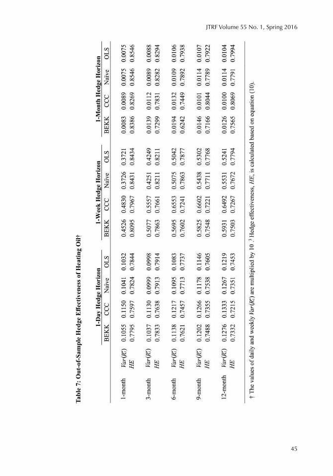
45


Tabl

e 7:

Out

-of-S

ampl

e H

edge

Effe

ctiv

enes

s of H

eatin

g O

il†


46

CONCLUSIONS

Because of wild swings in oil commodity prices, airlines undertake considerable risk with jet

fuel cross hedging. Ineffective hedges create substantial financial vulnerability and instability to airlines, which often incur considerable losses in their hedging programs. This paper examined the

effectiveness of WTI, Brent, gasoil, and heating oil as cross hedge proxies for jet fuel. The findings shed light on the effects of hedge duration and distance to maturity on hedge effectiveness. Our results show that heating oil is the most suitable proxy of the four oil commodities regardless of the

contract maturity and hedge horizon.

We find heating oil, rather than gasoil, to be a more suitable cross hedge proxy for jet fuel. This result contradicts the finding in Adams and Gerner (2012), which showed gasoil to be more superior. One plausible explanation for this is that Adams and Gerner (2012) used jet fuel spot prices from

Amsterdam-Rotterdam-Antwerp (ARA), which are likely more correlated with the future prices of

gasoil that is also traded in Europe (Adams and Gerner 2012). On the other hand, this study uses

U.S. Gulf Coast jet fuel as the spot market and considers No. 2 heating oil traded on the NYMEX as

a cross hedge commodity, thus heating oil is more suitable for U.S. jet fuel cross hedge. This may

indicate that besides the hedge horizon and distance to maturity, hedge effectiveness is also location-sensitive. We find gasoil’s performance to be the most inferior for a one-day holding period, but it improved considerably over a weekly horizon.

The out-of-sample results suggest that one- and three-month heating oil contracts are the most

desirable over contracts with longer maturities. This result is consistent with an earlier finding by Turner and Lim (2015). However, since Turner and Lim (2015) only assumed a one-day hedge

horizon, they did not examine the hedging performance over the weekly or monthly holding periods.

In this study, we find that a one-week horizon is more favorable than daily and monthly holding periods. Overall, the one-day hedge horizon is not recommended for all commodities and maturities,

and even though heating oil may be considered reasonably effective, the transaction costs associated with a daily horizon might be too high for the hedge to be considered economically sound.

In summary, the effects of hedging horizon and maturity on the performance of jet fuel proxies are commodity-specific. Heating oil outperforms all three other proxies, especially with a weekly hedge horizon and for contracts maturing in three months or less. Gasoil, WTI, and Brent all

perform well with a weekly hedge horizon, but their performances declined with a monthly hedge

horizon.

Acknowledgements

This study was funded in part by the Upper Great Plains Transportation Institute, North Dakota State

University, Fargo, North Dakota. We are grateful to two anonymous referees and Prof. Michael

Babcock, co-editor, for their constructive comments and suggestions.

47


Endnotes

1. Basis risk is the risk to a hedger as a result of the difference in the futures price and the spot price of a commodity.

2. A forward contract is a non-standardized contract between two parties that allow them to buy or sell an asset at a specific price at a specific time in the future. Unlike futures contracts that are exchange-traded, forward contracts are private agreements.

3. See Morrell and Swan (2006) for detailed discussions on futures, forwards, options, collars, and swaps.

4. In 2009, Ryanair’s fuel cost per available seat mile rose by 39% and total fuel cost rose by a

stunning 59% relative to the fuel costs in 2008 (Ryanair 2009).

5. Gasoil is the same as No. 2 fuel oil in the U.S., but it is the European designation for the product

and traded in Europe (Turner and Lim 2015).

6. A hedge ratio is the ratio of the size of a position in a financial contract, such as a futures contract, to the size of the underlying asset.

7. A long position refers to a firm’s position to buy an asset in the future, and a short position refers to a firm’s position to sell an asset in the future. If a firm takes a long cash position and a short futures position, that means the firm sells futures contracts while buying jet fuel in the spot market.

8. Baba, Engle, Kraft, and Kroner (BEKK 1990). The diagonal BEKK that restricts off-diagonal elements of the coefficient matrices to be zero, and is therefore more parsimonious than the general form BEKK.

9. Because gasoil futures price data for 12-month rolling contracts were not retrievable from

Bloomberg at the time of this research, we used the data for 11-month rolling contracts as a

proxy.

10. Results from the ADF and PP tests are consistent with those produced by the KPSS test. Hence,

the PP and ADF test results are not reported here.

11. Kurtosis measures the thickness of the tails of a distribution. A distribution with thick tails are

leptokurtic. In investment, a leptokurtic distribution means more risk as outlier events are more

likely to occur. Since the distribution of the GARCH residuals is leptokurtic, we assume the

distribution is Student’s t as opposed to normal.

References

Adams, Z., and M. Gerner. “Cross Hedging Jet-fuel Price Exposure.” Energy Economics 34 (5),

(2012): 1301 - 1309.

Argus. “Argus White Paper: Argus Jet Fuel Price Assessments.” available at: https://media.

argusmedia.com/~/media/Files/PDFs/White%20Paper/Jet-Fuel-Assessments.pdf (accessed 31 May

2013), 2012.

Baba, Y., R.F. Engle, D.F. Kraft, and K.F. Kroner. “Multivariate Simultaneous Generalized ARCH.”

Mimeo, Department of Economics, University of California – San Diego, 1990.


48

Baillie, R.T., and R.J. Myers. “Bivariate GARCH Estimation of the Optimal Commodity Futures

Hedge.” Journal of Applied Econometrics 6 (2), (1991): 109-124.

Bauwens, L., S. Laurent, and J.V.K. Rombouts. “Multivariate GARCH Models: A Survey.” Journal

of Applied Econometrics 21 (1), (2006): 79-109.

Bollerslev, T. “Modeling the Coherence in Short-run Nominal Exchange Rates: A Multivariate

Generalized ARCH Model.” Review of Economics and Statistics 72 (3), (1990): 498-505.

Brooks, R. “Samuelson Hypothesis and Carry Arbitrage.” Journal of Derivatives 20 (2), (2012):

37-65.

Cecchetti, S.G., R.E. Cumby, and S. Figlewski. “Estimation of Optimal Futures Hedge.” Review of

Economics and Statistics 70 (4), (1988): 623-630.

Chen, S.S., C.F. Lee, and K. Shrestha. “Futures Hedge Ratio: A Review.” The Quarterly Review of

Economics and Finance 43 (3), (2003): 433-465.

CME Group. “Derivatives and Hedge Accounting.” available at: http://www.cmegroup.com/

education/files/derivatives-and-hedge-accounting.pdf (accessed 1 March 2013), 2012.

Corley, M. “Mitigate Not Speculate.” Airline Economics 17, (2013): 74-75.

Ederington, L.H. “The Hedging Performance of the New Futures Markets.” Journal of Finance 34

(1), (1979): 157-170.

Engle, R.F., and K.F. Kroner. “Multivariate Simultaneous GARCH.” Econometric Theory 11 (3),

(1995): 122-150.

Finnerty, J.D., and D. Grant. “Alternative Approaches to Testing Effectiveness under SFAS No. 133.” Accounting Horizons 16 (2), (2002): 95-108.

Gronwald, M. “A Characterization of Oil Price Behavior- Evidence from Jump Models,” Energy

Economics 34 (5), (2012): 1310-1317.

Halls, M. “To Hedge or Not to Hedge.” AirfinanceJournal,(2005): 27-29.

Holmes, P. “Stock Index Futures Hedging: Hedge Ratio Estimation, Duration, Effects, Expiration Effects and Hedge Ratio Stability.” Journal of Business Finance and Accounting 23 (1), 1996: 63-

77.

Ledoit, O., P. Santa-Clara, and M. Wolf. “Flexible Multivariate GARCH Modeling with an

Application to International Stock Markets.” Review of Economics and Statistics 85 (3), (2003): 735-747.

Johnson, L.L. “The Theory of Hedging and Speculation in Commodity Futures.” Review of

Economic Studies 27 (3), (1960): 139-151.

Kroner, K.F., and J. Sultan. “Time-varying Distributions and Dynamic Hedging with Foreign

Currency Futures.” Journal of Financial and Quantitative Analysis 28 (4), (1993): 535-551.

Lien, D. “A Note on the Hedge Effectiveness of GARCH Models.” International Review of

Economics and Finance 18 (1), (2009): 110-112.

49


Lim, S.H., and Y. Hong. “Fuel Hedging and Airline Operating Costs.” Journal of Air Transport

Management 36, (2014): 33-40.

Lindahl, M. “Minimum Variance Hedge Ratios for Stock Index Futures: Duration and Expectation

Effects.” Journal of Futures Markets 12 (1), (1992): 33-53.

Malliaris, A.G., and J.L. Urrutia. “The Impact of the Lengths of Estimation Periods and Hedging

Horizons on the Effectiveness of a Hedge: Evidence from Foreign Currency Futures.” Journal of

Futures Market 11(3), (1991): 271-289.

Morrell, P., and W. Swan. “Airline Jet Fuel Hedging: Theory and Practice.” Transport Review 26

(6), (2006): 713-730.

Myers, R. “Estimating Time-varying Optimal Hedge Ratios on Futures Markets.” Journal of Futures

Markets 11 (1), (1991): 39-53.

Park, T.H., and L.N. Switzer. “Bivariate GARCH Estimation of the Optimal Hedge Ratios for Stock

Index Futures: A Note.” Journal of Futures Markets 15 (1), (1995): 61-67.

Rampini, A.A., A. Sufi, and S. Viswanathan. “Dynamic Risk Management.” Journal of Financial

Economics 111 (2), (2014): 271-296.

Ripple, R.D., and I. A. Moosa. “Hedge Effectiveness and Futures Contract Maturity: The Case of NYMEX Crude Oil Futures.” Applied Financial Economics 17 (9), (2007): 683-689.

Ryanair. “Annual Reports.” Available at: http://corporate.ryanair.com/investors/ (accessed 12

January 2013), (various years).

Samuelson, P.A “Proof That Properly Anticipated Prices Fluctuate Randomly.” Industrial

Management Review 6 (2), (1965): 41-49.

Southwest Airlines “Form 10K for the Fiscal Year Ending Dec 31, 2011 (Filing date: February 9,

2012).” Available at: http://www.investorroom.com (accessed January 23 2013), 2012.

Southwest Airlines. “Form 10K for the Fiscal Year Ending Dec 31, 2012 (Filing date: February 7,

2013).” Available at: http://www.investorroom.com (accessed May 4 2013), 2013.

Southwest Airlines. “Form 10K for the fiscal year ending Dec 31, 2014 (Filing date: February 6, 2015).” Available at: http://www.investorroom.com (accessed November 30 2015), 2015.

Turner, P.A., and S.H. Lim. “Hedging Jet Fuel Price Risk: The Case of U.S. Passenger Airlines.”

Journal of Air Transport Management 44, (2015): 54-64.

Zhang, H. “Effect of Derivative Accounting Rule on Corporate Risk Management Behavior.”

Journal of Accounting and Economics 47 (3), (2009): 244-264.

Siew Hoon Lim is an associate professor in the Department of Agribusiness and Applied Economics

at North Dakota State University. Her research interests are in transportation economics, production

economics, industrial organization and regional development. She received her Ph.D. in economics

from the University of Georgia.

Peter A. Turner received his M.S. in agribusiness and applied economics from North Dakota State

University.Hisresearchinterestisintransportationfinance.

transportation research forum · 11/30/2015 · airline fuel hedging 30 2011.4 the company’s low...

Documents