NBER WORKING PAPER SERIES

AN ECONOMIC ANALYSIS OF U.S AIRLINE FUEL ECONOMY DYNAMICSFROM 1991 TO 2015

Matthew E. KahnJerry Nickelsburg

Working Paper 22830http://www.nber.org/papers/w22830

NATIONAL BUREAU OF ECONOMIC RESEARCH1050 Massachusetts Avenue

Cambridge, MA 02138November 2016

We thank Alessandro Gavazza for sharing data with us. The views expressed herein are those of the authors and do not necessarily reflect the views of the National Bureau of Economic Research.

NBER working papers are circulated for discussion and comment purposes. They have not been peer-reviewed or been subject to the review by the NBER Board of Directors that accompanies official NBER publications.

© 2016 by Matthew E. Kahn and Jerry Nickelsburg. All rights reserved. Short sections of text, not to exceed two paragraphs, may be quoted without explicit permission provided that full credit, including © notice, is given to the source.

An Economic Analysis of U.S Airline Fuel Economy Dynamics from 1991 to 2015Matthew E. Kahn and Jerry NickelsburgNBER Working Paper No. 22830November 2016JEL No. L11,L62,R4

ABSTRACT

Airline transport generates a growing share of global greenhouse gas emissions but as of late 2016, this sector has not faced U.S. fuel economy or emissions regulation. At any point in time, airlines own and lease a set of durable vehicles and have invested in human and physical capital and an inventory of parts to maintain these vehicles. Each airline chooses whether to scrap and replace airplanes in their fleet and how to utilize and operate their fleet of aircraft. We model these choices as a function of real jet fuel prices. When jet fuel prices are higher, airlines fly fuel inefficient planes slower, scrap older fuel inefficient planes earlier and substitute miles flown to their more fuel efficient planes.

Matthew E. KahnDepartment of EconomicsUniversity of Southern CaliforniaKAPLos Angeles, CA 90089and NBERkahnme@usc.edu

Jerry NickelsburgUniversity of California, Los AngelesAnderson School of ManagementLos Angeles, CA 90095jerry.nickelsburg@anderson.ucla.edu

Introduction

Jet fuel is a major expense for commercial airlines. In 2014, the U.S civilian fleet

consumed 10.3 billion gallons for domestic flights. 1 At market prices this represented a total

expenditure of roughly $35 billion. This expense accounts for approximately 25% of operating

costs and therefore, these for-profit companies have strong incentives to manage their purchases

of such fuel.2

Fuel consumption represents a private cost for airlines and imposes externality costs for

society.3 Airplane travel is generating a growing share of global greenhouse gas emissions but

up as of 2016, this sector has not faced fuel economy regulation in the US. US aircraft are

emitting 11% of the total U.S transportation GHG emissions, and this represents 3% of total U.S

GHG emissions.4 Total greenhouse gas emissions per aircraft are proportional to its gallons per

mile consumed multiplied by total miles flown but differ by type of aircraft. The Airbus A320

aircraft now operated by United Airlines emits 59% of the CO2 as the previously operated

Boeing 727-200 during take-offs and landings.5 Therefore studying the impact of jet fuel prices

on this metric is informative for ascertaining the incidence of price policies designed to reduce

GHG emissions.

1 http://www.rita.dot.gov/bts/sites/rita.dot.gov.bts/files/publications/national_transportation_statistics/html/table_04_05.html 2 Fuel hedging by Southwest Airlines has become a case study at business schools. Scott Topping, Director of Corporate Finance at Southwest in 2001 stated that fuel prices have wrecked havoc in the airline industry. See for example: http://www.acumenalgo.com/wp-content/uploads/2015/11/SSRN-id578663.pdf 3 Representatives of 191 nations met in Montreal in September 2016 to discuss this externality, one that spans nations, and to develop potential mitigation policies. 4 https://www3.epa.gov/otaq/documents/aviation/420f15023.pdf 5Krysten Rypdal, Aircraft Emissions (Statistics Norway) http://www.ipcc-nggip.iges.or.jp/public/gp/bgp/2_5_Aircraft.pdf

Given that there is an environmental externality associated with air travel, it is surprising

how little academic economic research has investigated the fuel economy dynamics for this

important and growing transportation sector. In independent work, Abreu and Brueckner (2016)

document the negative correlation between airplane fuel consumption and gasoline prices.6 In

contrast, the fuel economy dynamics for the private automobile fleet and the public bus fleet

have been extensively studied (Knittel 2012).

We study U.S civilian airline fuel consumption dynamics by examining how airlines

utilize their existing set of planes that they own or lease at any point in time. Our measures of

utilization are miles flown and average speed. We document that plane utilization is responsive

to the jet fuel price of flying a mile. The jet fuel price of flying a passenger a mile is the product

of the price of jet fuel and the specific airplane’s gallons per passenger-mile. We document that

in years/quarters when the real jet fuel price is higher that airlines fly their less fuel efficient

airplanes less and they fly all planes at lower speeds to more efficiently use fuel.

Airlines can also replace their fleets and purchase newer more efficient airplanes. We

estimate fleet turnover regressions for the subset of aircraft at airlines when the fleets of those

aircraft are close to the margin of being replaced. We focus on major US airlines whose

inventory of planes features some older planes where a close more fuel efficient substitute exists.

We study whether fleet upgrading is more likely to occur when the price of jet fuel is higher and

thus the operating cost savings from upgrading to a more fuel efficient plane is higher. This piece

of our analysis updates earlier work by Goolsbee (1998) that focused on the retirement of the

Boeing 707 airplane during the 1970s and 1980s by using a larger portfolio of aircraft types and

more recent fleet data. 6 They report a negative correlation between miles flown and jet fuel prices. However, the short and long run operational outcomes are not part of their investigation.

The price of new aircraft and the lease rate for existing aircraft are both set in markets

featuring few sellers. During the period we study, 1991-2015, Airbus, Boeing and McDonnell

Douglas compete with leasing companies and owners of existing aircraft in highly developed

durable goods markets (Gavazza (2011)). The linkage between the used car and new car

markets is studied by Bento et. al. (2009). They document that new car regulation affects the

demand for used vehicles. As we discuss in the conclusion, this finding is likely to have

important implications for considering the incidence of new vintage airplane fuel economy

regulation.

We estimate hedonic used airplane pricing regressions to study the economic incidence of

higher jet fuel prices. We document that the lease price for fuel efficient airplanes is higher

when the price of jet fuel is higher. This fact means that airlines have a weaker incentive to

adjust to the higher fuel prices on the extensive margin. If plane purchasers anticipate that they

will face higher prices for fuel efficient planes when jet fuel prices are high then this provides an

incentive for them to engage in more adjustment along the intensive margin of mileage and

speed rather than at the extensive margin. This suggests that Gruenspecht’s predictions about the

consequences of differentiated regulation (where he focused on vehicles) is likely to play out in

the case of planes (Gruenspecht 1982).

Our study contributes to the transportation literature by examining how jet fuel prices

affect the fleet’s composition and utilization. Previous studies have documented how the fleet’s

average fuel economy is affected by gas prices (Li, Von Haefen and Timmins (2009), Linn and

Klier (2010)). Other vehicle research has examine how scrappage behavior is affected by

changes in gas prices (Jacobsen and Van Benthem (2014)).

An Airline’s Static Cost Minimization Problem

Airlines face a portfolio problem of what durables to own, and how much to use them.

For example in 1994, TWA operated 11 different types of aircraft from Douglas DC-9-10 to

Boeing 747-200. Each of these aircraft met a specific role, however at the margin similar aircraft

could substitute for each other. Airlines operate fleets comprised of multiple units of each type

of aircraft and they operate in a competitive environment as private firms (Borenstein (1992),

Goetz and Vowles (2009), Brueckner, Lee and Singer (2013). The replacement decision in this

setting represents a complicated dynamic programming problem. While Rust (1987) shows how

to study the bus engine replacement decision, the airline problem is much more complicated

because airlines own and lease multiple types of durable goods for which they must choose along

many dimensions including the number of seats per flight and the aircraft’s technical capabilities.

Facing this challenge, we focus on a static optimization problem. At any point in time t, a

commercial airline called d has signed long term rental contracts that locks it in to operate a

count of 𝑛𝑗𝑑𝑡 of airplanes of type j. This assumption means that we are studying the fleet

utilization decision independent of the fleet retirement and purchase decision. In a later section

of the paper, we will explore this extensive margin.

There are h different types of airplanes. This notation means that that airline d at time t

has available a total of ∑ 𝑛𝑗𝑑𝑡ℎ𝑗=1 airplanes. The airline has chosen to fly a given level of

aggregate passenger miles. It must choose how to allocate these planes to meet its aggregate

passenger mileage target. The aggregate passenger miles flown by airline d in year t equals:

𝑀𝑖𝑙𝑒𝑠𝑑𝑡 = ∑ 𝑛𝑗𝑑𝑡 ∗ 𝑚𝑖𝑙𝑒𝑠𝑗𝑑𝑡ℎ𝑗=1 (1)

Where 𝑚𝑖𝑙𝑒𝑠𝑗𝑑𝑡 is the average passenger miles that airline d flies each type of airplane j at time t.

Define 𝑠𝑝𝑒𝑒𝑑𝑗𝑑𝑡 as the average speed that airline d flies plane j at time t. Given this notation,

the total time required to fly these miles equals;

𝑇𝑖𝑚𝑒𝑑𝑡 = ∑ 𝑛𝑗𝑑𝑡 ∗ 𝑚𝑖𝑙𝑒𝑠𝑗𝑑𝑡/𝑠𝑝𝑒𝑒𝑑𝑗𝑑𝑡ℎ𝑗=1 (2)

Total fuel consumption equals;

𝐹𝑢𝑒𝑙 𝐶𝑜𝑛𝑠𝑢𝑚𝑝𝑡𝑖𝑜𝑛𝑑𝑡 = ∑ 𝑛𝑗𝑑𝑡 ∗ 𝑚𝑖𝑙𝑒𝑠𝑗𝑑𝑡 ∗ 𝐺𝑃𝑀𝑗𝑑𝑡ℎ𝑗=1 (3)

In equation (3), 𝐺𝑃𝑀𝑗𝑑𝑡 represents the gallons per passenger mile for airline d on plane j

at time t.

Given this notation, and our assumption that the firm has incurred a fixed cost of owning

or leasing its airplane fleet, airline d’s static variable cost minimization problem can be

expressed as:

min∑ 𝑤𝑎𝑔𝑒ℎ𝑑=1 ∗ 𝑇𝑖𝑚𝑒𝑑𝑡 + ∑ 𝑛𝑗𝑑𝑡 ∗ 𝑚𝑖𝑙𝑒𝑠𝑗𝑑𝑡 ∗ 𝐺𝑃𝑀𝑗𝑑𝑡ℎ

𝑗=1 (𝑠𝑝𝑒𝑒𝑑) ∗ 𝑃𝑟𝑖𝑐𝑒 𝑜𝑓 𝐺𝑎𝑠𝑡

(4) subject to:

𝑚𝑖𝑙𝑒𝑠𝑖𝑗𝑡 ≤ 𝐶𝑎𝑝𝑎𝑐𝑖𝑡𝑦𝑗

𝑀𝑖𝑙𝑒𝑠𝑑𝑡 = �𝑛𝑗𝑑𝑡 ∗ 𝑚𝑖𝑙𝑒𝑠𝑗𝑑𝑡

ℎ

𝑗=1

A given airline chooses the mileage and the speed of each of its planes. In equation (4),

the left term represents the total salaries paid to the pilots and staff. The term on the right

represents the airline’s total expenditure on fuel. For a given airplane type, gallons per mile is

an increasing function of plane speed. To avoid corner solutions, we introduce a capacity

constraint such that the most fuel efficient airplanes cannot fly all of the miles. We note that in

our simple setup, all planes of the same type will be used the same amount. Planes are

substitutes but are not perfect substitutes because they differ with respect to their fuel economy.

This simple model yields two comparative statics. First, higher gas prices cause airlines to fly

their lower GPM planes more and second, higher gas prices cause airlines to fly slower.7 We

recognize that our model does not include plane depreciation or maintenance expenditures.

The Empirical Framework

In our first set of empirical results, we study the portfolio reallocation problem as an

airline changes the share of miles it allocates to each type of plane to achieve its goal of

minimizing costs. Using the data we describe below, we calculate for each airplane type, its

average gallons per mile at a point in time. It is important to note that this is a weighted average

of all of the vintages of this type of plane currently flying (such as a 757-300). Since aircraft

manufacturers make relatively small changes to aircraft fuel economy over time, the average

vintage of the fleet will affect the average fuel burn of the fleet. 8

In equation (5), we present the algebra for how we calculate the gallons per mile for

plane type j in year t and quarter q for airline d.

𝐺𝑃𝑀𝑗𝑑𝑡𝑞 = ∑ 𝐺𝑃𝑀𝑗𝑑𝑙𝑡𝑞 ∗𝑘𝑙=1

𝑀𝑖𝑙𝑒𝑠𝑗𝑑𝑙𝑡𝑞𝑀𝑖𝑙𝑒𝑠𝑗𝑑𝑡𝑞

(5)

7 Northwest Airlines reported in 2008 that it saved 162 gallons of fuel per flight on Minneapolis to Paris runs by slowing the speed of the aircraft by 10 mph. http://www.dailymail.co.uk/news/article-563630/The-airline-slow-Pilots-told-fly-slower-save-fuel.html 8 For example, the introduction of winglets on the 737 in 2000 improved fuel efficiency of the aircraft and are more prevalent on more recent vintage aircraft.

This summation captures the fact that at any point in time an airline holds many different

types of planes and these planes differ with respect to their k vintages. Given our data, we

cannot disaggregate fuel economy by the vintage of a plane. We are able to calculate each

airline’s quarterly average fuel economy (gallons per mile) by airplane type.

We combine data on the real price of jet fuel in any year/quarter and the above measure

of airplane fuel economy, to calculate the real price of flying one passenger mile

𝐶𝑜𝑠𝑡 𝑜𝑓 𝐹𝑙𝑦𝑖𝑛𝑔 𝑂𝑛𝑒 𝑀𝑖𝑙𝑒𝑗𝑑𝑡𝑞 = 𝐺𝑃𝑀𝑗𝑑𝑡𝑞 ∗ 𝑃𝑟𝑖𝑐𝑒 𝑜𝑓 𝐺𝑎𝑠𝑡𝑞 (6)

As shown in equation (6) there are two sources of variation for the price of flying one

passenger mile. First, there is the fuel economy of the plane and second there is the real price of

gasoline in that year/quarter. We lag this variable by a quarter to avoid endogeneity concerns.

This is our key explanatory variable in the first set of regressions we report.

To test hypotheses related to the reallocation of airline miles across its fleet we estimate

versions of equation (7).

log (𝑚𝑖𝑙𝑒𝑠𝑗𝑑𝑡𝑞) = 𝜙𝑑𝑡𝑞 + 𝐵1 ∗ log�𝐶𝑜𝑠𝑡 𝑜𝑓 𝐹𝑙𝑦𝑖𝑛𝑔 𝑂𝑛𝑒 𝑀𝑖𝑙𝑒 𝑗𝑑𝑡𝑞−1� + 𝑈𝑗𝑑𝑡𝑞 (7)

As shown in equation (7) an airline d in year t and quarter q has h different types of

planes in its inventory. Such an airline contributes h observations to the regression. For each of

these h types of airplanes we observe the total count of passenger miles flown. We include a

rich set of fixed effects that we discuss below. The standard errors are clustered by year/quarter.

Given that flying at lower speeds saves on jet fuel consumption but increases flight times,

we study whether airlines fly their planes at a lower speed when the cost of flying a plane a

passenger mile increases.9 To test this hypothesis we regress the average speed of the aircraft

type by quarter on the cost of flying a passenger mile.

log (𝑠𝑝𝑒𝑒𝑑𝑗𝑑𝑡𝑞) = 𝜙𝑑𝑡𝑞 + 𝐵1 ∗ log�𝐶𝑜𝑠𝑡 𝑜𝑓 𝑓𝑙𝑦𝑖𝑛𝑔 𝑂𝑛𝑒 𝑃𝑎𝑠𝑠𝑒𝑛𝑔𝑒𝑟 𝑀𝑖𝑙𝑒 𝑗𝑑𝑡𝑞−1� + 𝑈𝑗𝑑𝑡𝑞

(8)

Airplane Data

Our airline data covers the years 1991 through the end of 2015. It is from statutory filings

by the airlines to the Bureau of Transportation Statistics.10 The data set is called the “T-2” data.

These data report aggregate statistics by airline/airplane/year/quarter. For example, one

observation will be United Airlines utilization of 747 aircraft in the 4th quarter of 2007. For this

observation, we observe the total miles flown by aircraft in this set, the hours it was in the air, the

total quantity of fuel consumed and the total passenger miles. Surprisingly, the data do not

indicate the count of airplanes in this set or the age of these airplanes. We use these data to

construct two key variables; gallons per mile which equals total gallons of gasoline consumed

divided by total passenger miles flown and average plane speed defined as total airplane miles

9 Grenelle, List and Metcalf (2016) report results from a field experiment in which pilots were nudged to fly at lower speeds. Such pilots responded by flying slower and this increased fuel economy and hence reduce aggregate greenhouse gas emissions.

10 http://www.transtats.bts.gov/Fields.asp?Table_ID=254

flown divided by total plane hours in the air. Our data source for gasoline prices is the BTS.11

We deflate these data and calculate an average quarterly real price of jet fuel per gallon.

Using the sample from the 1st quarter from 1991 through the 3rd quarter of 2015, after we

drop observations for which total jet fuel consumption equals zero or total passenger miles

equals zero, and we aggregate to the airline, plane type, year quarter level there are 16,276

observations in our unbalanced panel. These data cover 166 airlines, 132 airplanes over 99

year/quarters. The types of airlines in the data set are air taxi, charter, on demand cargo,

scheduled cargo, package cargo, regional and major airlines (airlines from 40 Mile Air to Yute

Air to United and American Airlines).

Figure One graphs the overall sample time trends in average gallons per mile, median

gallons per mile and the 90th percentile of the gallons per mile by calendar year. The mean and

median feature a constant linear trend. The 90th percentile declined sharply between 2000 and

2007. There have been other time periods such as 1996 to 2000 and 2008 to the present when

there have been no improvements in the 90th percentile’s fuel economy.

Figure Two presents a similar graph but this time we break out the data for three major

civilian airlines; American, Delta and United. While the three averages track each other closely,

Delta had the least fuel efficient planes at the start of the time period and by the end of the time

period, its planes were much more fuel efficient. In part this was due to the post-Northwest

merger decision to change its business model from fully integrated carrier to long haul carrier

with a feeder system. The new business model dictated efficient modern long range aircraft

dominating the fleet. In Figure Three, we graph the overall average time trend in gallons per

11 http://www.transtats.bts.gov/fuel.asp?pn=1

mile and we also graph the real price of jet fuel. There is no clear time series relationship

between these two series.

Results on Fleet Utilization and Speed as a Function of Operating Cost Per Mile

Table One reports three estimates of equation (7). We seek to explain the total mileage

of each airplane type for each airline in each year and quarter. The three regressions differ

because we include different sets of fixed effects. In column (1), we include carrier fixed

effects. In column (2), we include aircraft fixed effects and in column (3) we include

carrier/year/quarter fixed effects. This last set of fixed effects can be interpreted as flexibly

controlling for airline demand. In all three specifications, we estimate a negatively and

statistically significant elasticity for the real price of flying a passenger a mile. Based on the

results in column (3), we estimate an elasticity of -1.08. Thus, a 10% increase in the price of

flying a passenger mile reduces mileage for that plane by 10.8%. We recognize that our simple

reduced form approach does not allow us to estimate cross-elasticites which would be a

complicated adjustment throughout the airline’s portfolio of aircraft. As mileage on high GPM

planes declines, such miles may be reallocated to other airplanes that are part of the same

airline’s fleet.12

In Table Two, we report additional estimates of equation (7) but now we focus on the ten

major civilian airlines during our period of study and estimate a separate elasticity for each of

them. During the period of study America West and USAir merged, Northwest and Delta

merged, Continental and United merged and American purchased TWA. The airlines were kept

12 Since different airlines have different portfolios, the set of cross-elasticities will be airline specific. For example, an airline that only has three types of planes has fewer cross-elasticity adjustment margins than an airline that has seven different types of planes. Such a cross-elasticity research design would also have to explicitly incorporate capacity constraints because an airline could have seven different types of airplanes but just one plane of each type and this would limit its substitution possibilities.

as distinct entities prior to the merger. Fixed effects were used to judge whether or not the

merger changed airline strategy. For example, the predominance of Continental Airlines

management at the merged airline might be an example of the new United Airlines having a

different fleet strategy than before. We pursue this to test for heterogeneity. As shown in

Column (4), American Airlines and Southwest Airlines are the most responsive to changing

plane mileage as a function of the price of a passenger mile while US Airways is less responsive.

Table Three presents the airplane speed regressions based on equation (8). As shown in

Table Three’s column (3) the elasticities are negative but much smaller. We estimate a real

price per passenger mile elasticity of -.117 on plane speed.

Fleet Replacement and Jet Fuel Prices

In response to increases in fuel costs, airlines can also adjust their deployment of capital

by replacing an entire fleet of aircraft. For example Delta Airlines announced in April 2016 a

launch order for Bombardier C-Series aircraft for the purpose of improving operating economics

through the fuel burn economy of the new aircraft.

Airlines have infrastructure for each fleet that cannot be easily transferred across plane

types. For example, the firm incurs costs training pilots and mechanics in operating and repairing

a specific plane. The airline holds inventories of plane specific spare parts. Though these are

sunk costs, they are costs that must be borne whenever an entire fleet is replaced, and the

replacement and re-training costs add to the capital cost of a fleet rollover. For example, an

airline flying Boeing 737-300 aircraft might reduce the number of aircraft or reduce the

utilization in order to move traffic to a more efficient Boeing 757-200 aircraft, but were they to

replace this fleet with Airbus A320’s, a more efficient and similar sized aircraft, they would have

to retrain all of the 737-300 pilots. Pilot training alone requires two weeks of ground school,

fixed base device training and simulator sessions and can easily cost the airline $60,000 per pilot.

The acquisition of a flight simulator from CAE, FSI or TRU will cost $15M or more. United

Airlines operates 32 of these at its Denver training facility. Thus the gain from improved fuel

burn must be sufficiently large to trigger a fleet replacement decision.

We now present a simple fleet switching model that is used to guide our empirical

discrete choice model. A profit maximizing airline sells seats on its planes in a competitive

output market. Define 𝑆𝑡 as the Revenue Passenger Miles13 (RPM) provided at time t and St,k be

the RPM’s associated with aircraft type k. The ticket price for each flight is the sum or the

RPM’s times Pt,RPM. The airline wishes to produce RPM’s 𝑆𝑡 at each time t and has an infinite

lifetime objective function discounted by β. The production function for St is:

𝑆 = 𝑆(𝐿,𝐸|𝑉) = Σ𝑖𝑆𝑖,𝑡 (9)

In equation (1), 𝑉𝑡 be an overall fleet vintage (a and b aircraft fleets) at time t, 𝑃𝑡,𝑅𝑃𝑀 be the

ticket price per RPM at price t, 𝐿𝑡 be the amount of labor employed at t per RPM, 𝐸𝑡,𝑘 be the

amount of jet fuel consumed at t per RPM by aircraft k.

The firm bears costs in producing this quantity of passenger miles. Define 𝐶(𝑆𝑡 |𝑉𝑡 ) to

be the cost function for St

The state space representation of the objective function is:

Φ𝑡 = 𝑃𝑅𝑃𝑀𝑆𝑡 − 𝐶(𝑆𝑡 ) + 𝛽Φ𝑡+1 (10)

13 One RPM is one paying passenger carried one mile in flight

The airline’s problem at time t is:

𝑀𝑎𝑥{𝐿,𝑉,𝑅𝑃𝑀𝑘}{ 𝛷𝑡 } = 𝑃𝑡,𝑟𝑝𝑚𝑆𝑡(𝐿𝑡,𝐸𝑡|𝑉𝑡) − 𝐶( 𝑆𝑡|𝑉𝑡) + 𝛽 { 𝛷(𝑉𝑡+1)}, 𝑠. 𝑡. (11)

𝐶(𝑆𝑡 ) = 𝑤𝑡 𝐿𝑡 + 𝑃𝑡Σ𝑘𝐸𝑡,𝑘 + 𝑔𝑡Σ𝑘𝜇�𝑅𝑃𝑀𝑡,𝑘�𝐴𝑡,𝑘) + B𝑡,𝑘𝑖𝑡𝐼𝑡,𝑘 (12)

In this cost equation, 𝐵𝑡 be an indicator function = 0 if either no alternative more fuel efficient

aircraft is available, or if the airline decides not to include it in the fleet and =1 otherwise. 𝐴𝑡,𝑘 is

defined as the vintage of the type k aircraft fleet at time t. 𝑤𝑡 is the wage of labor at t. P𝑡 is the

price of jet fuel at t. 𝑖𝑡 is the corporate bond interest rate at t. 𝐼𝑡,𝑐 is the cost of new replacement

aircraft c. 𝜇(𝐴𝑡,𝑘) is the level of maintenance required for aircraft of type k.

Define 𝑔𝑡,𝑘 be the cost of maintenance per RPM for aircraft of type k. We assume that

maintenance costs 𝑔 is an increasing function of RPM’s in both vintage and current usage of the

aircraft:

𝜕𝑔(𝑅𝑃𝑀,𝐴)𝜕𝑅𝑃𝑀

> 0 𝑎𝑛𝑑 𝜕𝑔(𝑅𝑃𝑀,𝐴𝑡)𝜕𝐴𝑡

> 0.

An airline will choose to replace aircraft k with a new aircraft type r if an aircraft r exists

as an alternative and at the optimum without replacement:

𝑃𝑡,𝐸 � 𝜕𝐸

𝜕𝑅𝑃𝑀𝑘� + 𝑔𝑡 �

𝜕𝜇𝜕𝑅𝑃𝑀𝑘

� > 𝑃𝑡,𝐸 � 𝜕𝐸

𝜕𝑅𝑃𝑀𝑟� + 𝑔𝑡 �

𝜕𝜇𝜕𝑅𝑃𝑀𝑟

� + 𝑖𝑡𝐼𝑡,𝑟 (13)

From (13) we observe there are four ways this inequality can hold. First, the inequality holds

from the time the aircraft is available and the airline begins replacement as a launch customer for

the new efficient aircraft. Second, since the replacement aircraft is more fuel efficient than the

older aircraft (i.e. � 𝜕𝐸𝜕𝑅𝑃𝑀𝑟

� < � 𝜕𝐸𝜕𝑅𝑃𝑀𝑘

� ). Therefore an increase in energy prices 𝑃𝑡,𝐸 or expected

energy prices will increase the right hand side less than the left hand side and there exists a jet

fuel cost such that the inequality (14) holds. Third, as the aircraft fleet ages, it becomes more

expensive to operate (i.e. � 𝜕𝜇𝜕𝐴𝑡� < � 𝜕𝜇

𝜕𝐴𝑡+1� ). Thus, an aging fleet is less attractive than a new

fleet even if jet fuel prices do not increase. Finally, fleet replacement as a partial substitute for a

utilization adjustment between fleet types maybe induced by falling capital costs 𝑖𝑡𝐼𝑡,𝑘.

The discrete choice is then roll the fleet into a new type or keep the existing fleet. We

model the probability of this choice as:

𝑝𝑟𝑜𝑏(𝑓𝑙𝑒𝑒𝑡 𝑟𝑒𝑝𝑙𝑎𝑐𝑒𝑘𝑖𝑡) = 𝑓(𝐵1 ∗ 𝑣𝑖𝑛𝑡𝑎𝑔𝑒𝑘𝑖𝑡 + 𝐵2 ∗ 𝑍𝑖𝑗𝑡 + 𝐵3 ∗ 𝑋𝑘𝑖𝑡) (14)

Where 𝑍𝑖𝑗𝑡 = log (𝑗𝑒𝑡 𝑓𝑢𝑒𝑙𝑡 ∗ ∆𝑓𝑢𝑒𝑙 𝑐𝑜𝑛𝑠𝑢𝑚𝑝𝑡𝑖𝑜𝑛 𝑝𝑒𝑟 𝑚𝑖𝑙𝑒𝑖𝑗𝑡)

In this last term, the change in fuel consumption per mile of flying represents the change in

consumption when airline k substitutes from plane i to j.

We posit that 𝐵1 will have a positive sign reflecting the increased maintenance costs

associated with aging aircraft. 𝐵2 is the coefficient of interest. The replacement aircraft will

have a lower fuel burn / mile than the existing aircraft. Jet fuel prices are positive and therefore

any aircraft pair, the variable will be a larger negative the higher are jet fuel prices. From the

model we expect this to increase the probability that airlines replace their fleets of relatively fuel

efficient with relatively more fuel efficient aircraft (equation 14). Our hypothesis is then that

𝐵2will be negative and significant.

Fleet Replacement Data

The data employed are airline fleets as constructed from historical records of each of ten

airlines including the average age and number of aircraft of the fleet. Maintenance cost data

were not available on a consistent basis as each aircraft’s maintenance cost is dependent on the

number of hours flown, the number of cycles flown and the age of the aircraft. Nevertheless, the

age of the fleet is a good proxy for this variable.

The data for the empirical study are comprised of annual counts of aircraft in the fleets of

the top ten domestic airlines from 1991 to 2014. For each fleet the first five years after an

aircraft has entered the airline are considered adoption times and are not included in the data.

Aircraft for which there are no more fuel efficient alternatives, are also excluded from the data.

The date used for the fleet replacement decision is the year of entry of the first aircraft of the

new, replacement fleet. While airlines decide to roll a fleet considerably in advance of the first

delivery, the market for leased aircraft and the nature of new aircraft purchase contracts allows

them considerable flexibility in the actual date to begin the fleet rollover. Thus, the introduction

to the fleet date is taken as the relevant decision date.

The key variables we construct include;

1. Fleet Replacement: a binary choice variable taking the value of 1 when a fleet replacement occurs and 0 otherwise. The data consists of airline fleets that have been in the airline for at least five years as the empirical data suggests that airlines do not replace fleets without operating them for at least five years.

2. Vintage: the average age of the fleet. As fleets age maintenance cost increase. As well, minor changes in aircraft result in improvements in fuel burn and younger fleets will be marginally more fuel efficient than older fleets.

3. Fleet Total: The percentage of the airline’s aircraft that are in the subject fleet. 4. Chapter 11: A binary variable indicating the airline is in Chapter 11 bankruptcy

reorganization 5. Recession: a binary variable indicating the US is in a recession 6. Log(( real price of jet fuel) x (fuel burn in gallons per mile of the potential alternative

aircraft type - fuel burn in gallons per mile of the existing aircraft type)). This variable is a measure of the fuel savings per revenue mile achieved at current jet fuel prices by switching from the existing aircraft to a comparable fuel efficient aircraft. Fore example, an airline flying a McDonnell Douglas MD-83 aircraft might switch to a more fuel efficient Airbus A320-200 aircraft. This variable measures the increased cost incurred by the airline by not doing so.

The last variable is the key variable of interest. If the second argument of this transformation is

negative an increase in the real price of jet fuel will make this variable take on a more negative

value.

Fleet Replacement Results

At the extensive margin, airlines are responding to jet fuel price increases. Using the

fleet data for ten US airlines from 1992 to 2014 we estimated Probit models of the probability of

fleet replacement. The date of the fleet replacement was taken to be the year of introduction of

the new aircraft type. The Probit models were estimated with year and with airline fixed effects.

We find that when suitable substitutes exist, a 1% increase in jet fuel prices results in

approximately 1% increase in the probability of a fleet replacement. For airlines with older

fleets the probability of fleet replacement increases as well. This is expected as older fleets

require more maintenance. However they also have higher fuel burn. An increase of one year,

from 10 to 11 years, will increase the probability of replacement by approximately 2 percentage

points.14

An interesting result is that an airline in Chapter 11 bankruptcy is 14% more likely to roll

a fleet than one that is not. This is because of the deep lease market that allows airlines to adjust

their inputs at the extensive margin to reduce operating costs. Typically a bankrupt airline would

shrink its overall fleet by retiring older aircraft and add fewer, but more fuel efficient aircraft in

their place. While such a change in the fleet is costly, the Chapter 11 airlines are able to do it at

14 In the specifications without year fixed effects, the jet fuel price is estimated to be an important determinate of the fleet rollover decision. A quadratic specification was preferred as it captures the differential impact of high and low jet fuel prices.

lower cost than non-Chapter 11 airlines due to the concomitant contraction of their fleet, the

potential for debtor-in-possession financing and the potential suspension of other obligations.

Aircraft Lease Prices and a Hedonic Test of the Incidence of Jet Fuel Price Changes

When gasoline prices are high, airlines seek out more fuel efficient planes. Such demand

may raise the equilibrium prices for such planes. We now introduce an econometric

specification that resembles the approach taken by Busse et. al. (2013) and Fan, Sallee and West

(2016) in their studies of the capitalization of gasoline prices into used vehicle prices. We use

standard hedonic pricing methods to study the economic incidence of higher gas prices. In

particular we will study whether and to what extent planes featuring higher jet fuel costs per

passenger mile are associated with lower lease rate and rental rates. Intuitively, if a plane has a

high gallons per mile then its operating costs rise as the price of gasoline increases. The variable

“cost of flying one passenger mile” captures this. In running the hedonic regression below, we

are assuming that airlines are using today’s jet fuel price as a proxy for future jet fuel prices. If

such prices follow a random walk, then this assumption is costless.

In equation (15), the unit of analysis is plane j built in year v sales price in year t

log (𝑝𝑟𝑖𝑐𝑒𝑗𝑣𝑡) = 𝐵1 ∗ 𝑋𝑗𝑣𝑡 + 𝐵2 ∗ log (𝐶𝑜𝑠𝑡 𝑜𝑓 𝑓𝑙𝑦𝑖𝑛𝑔 𝑂𝑛𝑒 𝑃𝑎𝑠𝑠𝑒𝑛𝑔𝑒𝑟 𝑀𝑖𝑙𝑒𝑗𝑣𝑡) + 𝑈𝑗𝑣𝑡

(15)

The hedonic regressions are performed on data by aircraft type for the years 1991 to

2009. The data are the same as used by Gavazza (2010, 2011). The characteristics of the aircraft

are from Airliners.net and are the average for the fleet (e.g. the number of seats is taken to be the

“typical 2 class” configuration). The characteristics are price of gasoline multiplied by the

gallons of jet fuel per passenger mile, number of seats, maximum gross take-off weight, range,

number of engines, and vintage of the aircraft.

The hedonic estimates are reported in Table Five. This table reports four hedonic

estimates of equation (15). The left columns use the lease price data and the right columns use

the sales price data. The regressions differ because airplane fixed effects are included in

columns (2) and (4). Across the four specifications, we find a large negative statistically

significant elasticity on the log of the jet fuel price of flying a passenger mile of -.61 in the lease

regressions and -1.3 in the sales price regressions. This indicates that the market valuation is

capitalizing operating cost expenses.

To quantify the incidence of the fuel price increases, we simulate the model for

alternative wide-body aircraft over a range of years and with a 1% increase in fuel prices. The

results are presented in Figure Four. To standardize the results, lease rates have been adjusted

for changes in interest rates. There is a high degree of variability in incidence reflecting the

interaction between competitive aircraft, the size of the market and the increased operating costs

of the particular aircraft. We find that a third to a half of the increase in fuel prices to be borne

by the aircraft lessor and the balance by the lessee.

Given that we have presented evidence that market prices for fuel efficient airplanes are

negatively correlated with gas prices, this provides an incentive for domestic airlines to focus

more of their adaptation efforts on the intensive margins of mileage and speed for their

incumbent fleet.

Conclusion

Over the last 25 years, U.S commercial airlines responded to higher real jet fuel prices by

flying more fuel-efficient planes more, flying aircrafts at slower speeds and upgrading their fleets

to more fuel-efficient planes. These findings add to the growing literature on how the

transportation sector responds to gas price dynamics.

In our recent work, we have studied how public bus authorities adapted to changing

gasoline prices (Kahn, Li and Nickelsburg (2015)). By now introducing new findings for fleets

of private civilian airplanes, we offer new facts for comparing these different capital stocks and

the policy implications of utilizing pricing dynamics for reducing aircraft emissions.

While all civilian airlines, public buses and private vehicles all provide transportation

services, they each differ with respect to who is making the decision -- households versus quasi-

governmental firms versus private sector firms – and to what are the underlying objective

function and constraints – individual utility, public provision of services and profit. A key

difference between the household’s utility maximizing decision over mileage across its portfolio

and the airline’s profit maximization problem is that airlines have greater substitution

possibilities at the intensive margin for substituting among the planes they already own and have

leased. But, at the same time airlines face significant adjustment costs at the extensive margin

because they must have inventories of spare parts, capital equipment for maintenance and

training, retraining costs and they must have trained mechanics with requisite expertise in

operating and repairing the aircraft most of the airports the aircraft services. Individual

households can outsource such services to repair stores.

Our findings on the behavioral responses of airlines to the changing price of flying a

passenger mile are relevant for policy decisions today because the Obama Administration seeks

to push through CAFE like plane regulations that will sharply increase the fuel economy of new

planes15 and the EU is increasing its regulation of aircraft emissions.16 If such regulations are

effective at reducing new plane emissions per mile, then our hedonic pricing results suggest that

such airplane sellers will sell these new planes at higher prices. This will reduce the demand for

such new planes and will benefit airlines holding portfolios of fuel efficient planes. Those

airlines and asset holders holding fuel inefficient planes will suffer a capital loss through the

capitalization effect that we documented using our hedonic regressions.

An open question that would require a structural modeling approach would be to study

how new plane fuel economy regulations affects the pricing of future airplanes. At present

airlines have only two large transport manufacturers to choose from. The emergence of

Bombardier, Embraer, and Mitsubishi as manufacturers of competitive aircraft at the lower end

of the capacity spectrum may induce more competition. Lufthansa and Delta orders for

Bombardier C-Series has already eaten into the big-two’s market share in the 100 to 150 seat

segment.

Nevertheless, as new planes become more expensive (due to new differentiated capital

regulation), our results suggest that airlines will substitute at the intensive margin to keeping

their existing older airplanes for longer than they would have absent the capitalization of the fuel

saving or emissions gain. Gruenpshect (1982) posits that such differentiated regulation can

15 https://www.whitehouse.gov/the-press-office/2016/02/08/fact-sheet-us-leadership-securing-first-ever-global-carbon-emissions 16 https://ec.europa.eu/clima/policies/transport/aviation/index_en.htm

actually increase pollution in the short run due to this vintage substitution effect. Testing this

prediction for the airline sector merits future research.

References

Allcott H, Wozny N. Gasoline prices, fuel economy, and the energy paradox. Review of Economics and Statistics. 2014 Dec 1;96(5):779-95. Abreu, Chrystyane and Jan Brueckner. Airline Fuel Usage and Carbon Emissions: Determining Factors. UC Irvine Working Paper June 2016. Bento AM, Goulder LH, Jacobsen MR, Von Haefen RH. Distributional and efficiency impacts of increased US gasoline taxes. The American Economic Review. 2009 Jun 1;99(3):667-99. Beresteanu A, Li S. Gasoline prices, government support, and the demand for hybrid vehicles in the United States. International Economic Review. 2011 Feb 1;52(1):161-82. Borenstein, Severin. "The Evolution of U.S. Airline Competition." The Journal of Economic Perspectives 6, no. 2 (1992): 45-73. Brueckner, Jan, Darin Lee, and Ethan S. Singer. Airline competition and domestic US airfares: A comprehensive reappraisal. Economics of Transportation. Volume 2, Issue 1, March 2013, Pages 1–17.

Busse MR, Knittel CR, Zettelmeyer F. Are consumers myopic? Evidence from new and used car purchases. The American Economic Review. 2013 Feb 1;103(1):220-56. Espey M, Nair S. Automobile fuel economy: What is it worth?. Contemporary Economic Policy. 2005 Jul 1;23(3):317-23.

Fan, Wei, James Sallee and Sarah West. Do Consumers Recognize the Value of Fuel Economy? Evidence from Used Car Prices and Gasoline Price Fluctuations, Journal of Public Economics 2016. 135, 61-73.

Gavazza Alessandro. Asset liquidity and financial contracts: Evidence from aircraft leases. Journal of Financial Economics. 2010 Jan 31;95(1):62-84.

Gavazza Alessandro. Leasing and secondary markets: Theory and evidence from commercial aircraft. Journal of Political Economy. 2011 119(2) 325-377

Goetz, Andrew R. and Timothy M. Vowles. The good, the bad, and the ugly: 30 years of US airline deregulation. Journal of Transport Geography. Volume 17, Issue 4, July 2009, Pages 251–263 Gillingham, Kenneth, Chris Knittel and David Rapson. The Household Vehicle Portfolio: Implications for Emissions Abatement Policies”

Goolsbee A. The business cycle, financial performance, and the retirement of capital goods. Review of Economic Dynamics. 1998 Apr 30;1(2):474-96.

Gosnell GK, List JA, Metcalfe RD. A New Approach to an Age-Old Problem: Solving Externalities by Incenting Workers Directly. NBER Working Paper 22316 2016.

Gruenspecht HK. Differentiated regulation: The case of auto emissions standards. The American Economic Review. 1982 May 1;72(2):328-31.

Jacobsen, Mark R. and Arthur A. van Benthem. 2015. "Vehicle Scrappage and Gasoline Policy." American Economic Review, 105(3): 1312-38. Knittel CR. Reducing petroleum consumption from transportation. The Journal of Economic Perspectives. 2012 Jan 1;26(1):93-118. Li S, Von Haefen R, Timmins C. How do gasoline prices affect fleet fuel economy?. American Economic Journal: Economic Policy 2009, 1:2, 113–137 Li S, Kahn ME, Nickelsburg J. Public transit bus procurement: The role of energy prices, regulation and federal subsidies. Journal of Urban Economics. 2015 May 31;87:57-71. Linn, Joshua, and Thomas Klier. 2010. “The Price of Gasoline and the Demand for Fuel Efficiency: Evidence from Monthly New Vehicles Sales Data.” American Economic Journal: Economic Policy 2(3) 134-153. Rust J. Optimal replacement of GMC bus engines: An empirical model of Harold Zurcher. Econometrica: Journal of the Econometric Society. 1987 Sep 1:999-1033.

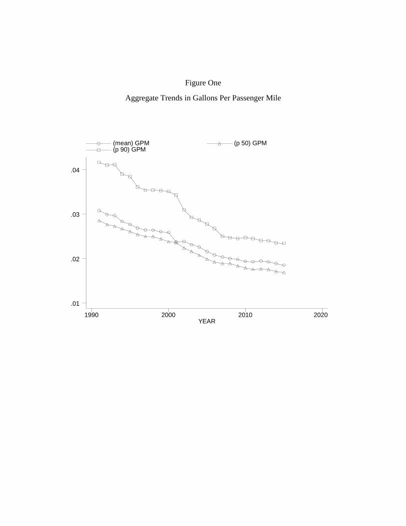
Figure One

Aggregate Trends in Gallons Per Passenger Mile

YEAR

(mean) GPM (p 50) GPM (p 90) GPM

1990 2000 2010 2020

.01

.02

.03

.04

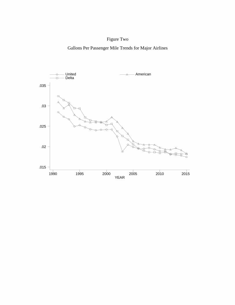
Figure Two

Gallons Per Passenger Mile Trends for Major Airlines

YEAR

United American Delta

1990 1995 2000 2005 2010 2015

.015

.02

.025

.03

.035

Figure Three

Table One

Passenger Miles as a Function of Energy Operating Costs

Y=log(miles flown by airline/year/quarter/airplane type)(1) (2) (3)

log(price per passenger mile) -0.702*** -0.859*** -1.083***(0.048) (0.076) (0.058)

Constant 16.141*** 16.458*** 15.481***(0.125) (0.223) (0.201)

Observations 15,877 15,877 15,877R-squared 0.795 0.645 0.853

*** p<0.01, ** p<0.05, * p<0.1

Fixed EffectsYear Y N YAirline Y Y YAircraft N Y NQuarter N N Y

Robust standard errors in parentheses. Standard errors clustered by year/quarter

Table Two

Passenger Miles by Major Airline as a Function of Energy Operating Costs

American Airlines is the omitted category.

(1) (2) (3) (4)

log(price per passenger mile) = X -1.907*** -1.801*** -0.885*** -2.256***(0.108) (0.126) (0.142) (0.177)

Continental * X 0.137 0.320 0.498(0.449) (0.198) (0.715)

Delta *X 0.043 -0.143 0.401(0.179) (0.168) (0.261)

America West* X -0.580** 0.429 -0.316(0.250) (0.274) (0.325)

Northwest *X -0.387*** 0.276* -0.032(0.140) (0.160) (0.174)

TWA * X -0.365** 0.433*** -0.223(0.147) (0.136) (0.219)

United * X -0.148 -0.117 -0.051(0.196) (0.174) (0.316)

US Air *X 0.241 0.231 0.685*(0.247) (0.155) (0.360)

Southwest*X -0.836*** -0.746*** -1.895***(0.209) (0.210) (0.406)

Constant 13.385*** 13.383*** 17.863*** 12.759***(0.395) (0.356) (0.556) (0.440)

Observations 6,774 6,774 6,774 6,774R-squared 0.386 0.391 0.605 0.459

*** p<0.01, ** p<0.05, * p<0.1

Fixed EffectsYear Y Y Y Y Airline Y Y Y YAircraft N N Y NQuarter N N N Y

Y=log(miles flown by airline/year/quarter/airplane type)

Robust standard errors in parentheses. Standard errors clustered by year/quarter

Table Three

Aircraft Speed as a Function of Energy Operating Costs

(1) (2) (3)

1991 omittedlog(price per passenger mile) -0.083*** -0.054*** -0.117***

(0.010) (0.008) (0.012)Constant 5.651*** 5.794*** 5.566***

(0.032) (0.029) (0.043)

Observations 15,665 15,665 15,665R-squared 0.434 0.524 0.714

*** p<0.01, ** p<0.05, * p<0.1

Fixed EffectsYear Y N YAirline Y Y YAircraft N Y NQuarter N N Y

Y=log(Aircraft Speed)

Robust standard errors in parentheses. Standard errors clustered by year/quarter

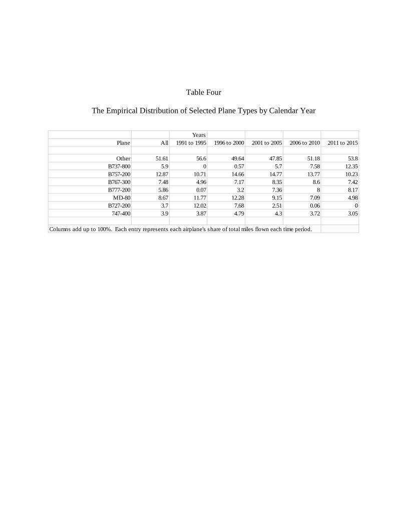
Table Four

The Empirical Distribution of Selected Plane Types by Calendar Year

YearsPlane All 1991 to 1995 1996 to 2000 2001 to 2005 2006 to 2010 2011 to 2015

Other 51.61 56.6 49.64 47.85 51.18 53.8B737-800 5.9 0 0.57 5.7 7.58 12.35B757-200 12.87 10.71 14.66 14.77 13.77 10.23B767-300 7.48 4.96 7.17 8.35 8.6 7.42B777-200 5.86 0.07 3.2 7.36 8 8.17

MD-80 8.67 11.77 12.28 9.15 7.09 4.98B727-200 3.7 12.02 7.68 2.51 0.06 0

747-400 3.9 3.87 4.79 4.3 3.72 3.05

Columns add up to 100%. Each entry represents each airplane's share of total miles flown each time period.

Table Five

The Fleet Replacement Decision

Probit Regressions Fleet Replacement by a more fuel efficient aircraft of the same gauge

(1) (2) (3) (4) (5) (6) (7) (8)

Vintage 0.0161 0.2157*** 0.0109 0.1701*** 0.0339*** 0.1986*** 0.0390*** 0.2257***(0.0117) -0.0665 (.0101) (0.0594) (0.0115) (0.5867) (0.0134) (0.0689)

Vintage Squared -0.0052*** -0.0039*** -0.0037*** -.0044**(0.0017) (0.0015) (0.0014) (0.0018)

Fleet as % of Total -1.0592 -0.8987 -0.9502 -0.6358 -1.6053 -1.3504 -1.8364 -1.6214(1.0040) (1.0657) (0.9047) (0.9268) (1.0549) (1.0833) (1.1855) (1.2504)

Chapter11 0.6987** 0.8189** .7284*** 0.8021*** 1.1435*** 1.1981*** 1.0699*** 1.1545***(0.3122) (0.3315) (0.2433) (0.2567) (0.2930) (0.3046) (0.3581) (0.3777)

Recession 4.0765 4.2198 0.3170 0.3283 0.4188 0.4351 3.1651 2.9948(192.5) (172.1) (0.2507) (0.2610) (0.2728) (0.2827) (207.7) (150.40

Log(PricexFuel burn differential) 0.1704 -1.1693* -0.2063 -0.3621** -0.5448*** -0.6580*** -0.1373 -1.1914(0.4068) (0.8960) (0.1370) (0.1756) (0.1792) (0.2154) (0.4742) (0.9750)

Log(PricexFuel burn differential) squared -1.1194** -0.2491 -0.1992 -0.7179(0.5356) (0.2005) (0.2175) (0.6005)

Airline Fixed Effects N N N N Y Y Y YYear Fixed Effects Y Y N N N N Y YObservations 537 537 537 537 537 537 537 537χ2-Statistic 30.60 62.27 30.6 44.59 39.75 51.36 55.29 67.46Standard errors in parentheses*** p<0.01, ** p<0.05, * p<0.1

Table Six

Hedonic Airplane Valuation Regressions

Log(Y)(1) (2) (3) (4)

log(price per passenger mile) -0.6128*** -0.2008* -1.3050*** -0.6565***(0.1464) (0.1146) (0.2297) (0.1650)

Age of Aircraft -0.0530*** -0.0633*** -0.0946*** -0.1142***(0.0061) (0.0049) (0.0104) (0.0114)

Maximum Aircraft Weight (100s) 0.0002* 0.0000 0.0002* -0.0001***(0.0001) (0.0000) (0.0001) (0.0000)

Number of Seats 0.0013 0.0018(0.0011) (0.0017)

Mileage Range 0.0438 -0.0050(0.0494) (0.0752)

Number of Engines -0.2648* -0.3961*(0.1512) (0.2307)

Constant 3.6096*** 5.6265*** -0.6008 2.8882***(0.8134) (0.3175) (1.2707) (0.5920)

Observations 5,659 5,659 5,659 5,659R-squared 0.8314 0.8990 0.8051 0.8705Robust standard errors in parenthesesStandard errors clustered by airplane type*** p<0.01, ** p<0.05, * p<0.1

Fixed EffectYear Y Y Y YAirplane N Y N Y

Lease Price Purchase Price