advanced methods in meta-analysis: multivariate approach and

STATISTICS IN MEDICINEStatist. Med. 2002; 21:589–624 (DOI: 10.1002/sim.1040)

TUTORIAL IN BIOSTATISTICSAdvanced methods in meta-analysis: multivariate approach

and meta-regression

Hans C. van Houwelingen1;∗;†, Lidia R. Arends2 and Theo Stijnen2

1Department of Medical Statistics; Leiden University Medical Center; P.O. Box 9604; 2300 RC Leiden;The Netherlands

2Department of Epidemiology & Biostatistics; Erasmus Medical Center Rotterdam; P.O. Box 1738;3000 DR Rotterdam; The Netherlands

SUMMARY

This tutorial on advanced statistical methods for meta-analysis can be seen as a sequel to the recentTutorial in Biostatistics on meta-analysis by Normand, which focused on elementary methods. Withinthe framework of the general linear mixed model using approximate likelihood, we discuss methodsto analyse univariate as well as bivariate treatment e<ects in meta-analyses as well as meta-regressionmethods. Several extensions of the models are discussed, like exact likelihood, non-normal mixtures andmultiple endpoints. We end with a discussion about the use of Bayesian methods in meta-analysis. Allmethods are illustrated by a meta-analysis concerning the e=cacy of BCG vaccine against tuberculosis.All analyses that use approximate likelihood can be carried out by standard software. We demonstratehow the models can be ?tted using SAS Proc Mixed. Copyright ? 2002 John Wiley & Sons, Ltd.

KEY WORDS: meta-analysis; meta-regression; multivariate random e<ects models

1. INTRODUCTION

In this paper we review advanced statistical methods for meta-analysis as used in bivariatemeta-analysis [1] (that is, two outcomes per study are modelled simultaneously) and meta-regression [2]. It can be seen as a sequel to the recent Tutorial in Biostatistics on meta-analysisby Normand [3]. Meta-analysis is put in the context of mixed models using (approximate)likelihood methods to estimate all relevant parameters. In the medical literature meta-analysisis usually applied to the results of clinical trials, but the application of the theory presented inthis paper is not limited to clinical trials only. It is the aim of the paper not only to discussthe underlying theory but also to give practical guidelines how to carry out these analyses.As the leading example we use the meta-analysis data set of Colditz et al. [4]. This data set

is also discussed in Berkey et al. [2]. Wherever feasible, it is speci?ed how the analysis can

∗Correspondence to: Hans C. van Houwelingen, Department of Medical Statistics, Leiden University MedicalCenter, P.O. Box 9604, 2300 RC Leiden, The Netherlands

†E-mail: [email protected] December 1999

Copyright ? 2002 John Wiley & Sons, Ltd. Accepted June 2001

590 H. C. VAN HOUWELINGEN, L. R. ARENDS AND T. STIJNEN

be performed by using the SAS procedure Proc Mixed. The paper is organized as follows. InSection 2 we review the concept of approximate likelihood that was introduced in the meta-analysis setting by DerSimonian and Laird [5]. In Section 3 we review the meta-analysisof one-dimensional treatment e<ect parameters. In Section 4 we discuss the bivariate ap-proach [1] and its link with the concept of underlying risk as source of heterogeneity [6–10]. InSection 5 we discuss meta-regression within the mixed model setting. Covariates consideredare aggregate measures on the study level. We do not go into meta-analysis with patient-speci?c covariates. In principle that is not di<erent from analysing a multi-centre study [11].In Section 6 several extensions are discussed: exact likelihood’s based on conditioning; non-normal mixtures; multiple endpoints; other outcome measures, and other software. This isadditional material that can be skipped at ?rst reading. Section 7 is concerned with the useof Bayesian methods in meta-analysis. We argue that Bayesian methods can be useful if theyare applied at the right level of the hierarchical model. The paper is concluded in Section 8.

2. APPROXIMATE LIKELIHOOD

The basic situation in meta-analysis is that we are dealing with n studies in which a parameterof interest #i (i=1; : : : ; n) is estimated. In a meta-analysis of clinical trials the parameter ofinterest is some measure of the di<erence in e=cacy between the two treatment arms. Themost popular choice is the log-odds ratio, but this could also be the risk or rate di<erence orthe risk or rate ratio for dichotomous outcome or similar measures for continuous outcomesor survival data. All studies report an estimate #̂i of the true #i and the standard error si of theestimate. If the studies only report the estimate and the p-value or a con?dence interval, wecan derive the standard error from the p-value or the con?dence interval. In the Sections 3to 5, which give the main statistical tools, we act as if #̂i has a normal distribution withunknown mean #i and known standard deviation si, that is

#̂i ∼ N(#i; s2i ) (1)

Moreover, since the estimates are derived from di<erent data sets, the #̂i are conditionallyindependent given #i. This approximate likelihood approach goes back to the seminal paperby DerSimonian and Laird [5]. However, it should be stressed that it is not the normality ofthe frequency distribution of #̂i that is employed in our analysis. Since our whole approachis likelihood based, we only use that the likelihood of the unknown parameter in each studylooks like the likelihood of (1). Thus, if we denote the log-likelihood of the ith study by‘i(#), the real approximation is

‘i(#)=− 12(#− #̂i)2=s2i + ci (2)

where ci is some constant that does not depend on the unknown parameter.If in each study the unknown parameter is estimated by maximum likelihood, approximation

(2) is just the second-order Taylor expansion of the (pro?le) log-likelihood around the MLE#̂i. The approximation (2) is usually quite good, even if the estimator #̂i is discrete. Sincemost studies indeed use the maximum likelihood method to estimate the unknown parameter,we are con?dent that (2) can be used as an approximation. In Section 6 we will discuss

Copyright ? 2002 John Wiley & Sons, Ltd. Statist. Med. 2002; 21:589–624

ADVANCED METHODS IN META-ANALYSIS 591

some re?nements of this approximation. In manipulating the likelihoods we can safely act asif we assume that (1) is valid and use, for example, known results for mixtures of normaldistributions. However, we want to stress that actually we only use assumption (2).The approach of Yusuf et al. [12], popular in ?xed e<ect meta-analysis, and of Whitehead

and Whitehead [13] are based on a Taylor expansion of the log-likelihood around the value#=0. This is valid if the e<ects in each study are relatively small. It gives an approximation inthe line of (2) with di<erent estimators and standard errors but a similar quadratic expressionin the unknown parameter.As we have already noted, the most popular outcome measure in meta-analysis is the log-

odds ratio. Its estimated standard error is equal to ∞ if one of the frequencies in the 2× 2table is equal to zero. That is usually repaired by adding 0.5 to all cell frequencies. We willdiscuss more appropriate ways of handling this problem in Section 6.

3. ANALYSING ONE-DIMENSIONAL TREATMENT EFFECTS

The analysis under homogeneity makes the assumption that the unknown parameter is exactlythe same in all studies, that is #1 =#2 = · · · =#n=#. The log-likelihood for # is given by

‘(#)=∑i‘i(#)=−1

2∑i[(#− #̂i)2=s2i + ln(s

2i ) + ln(2�)] (3)

Maximization is straightforward and results in the well-known estimator of the common e<ect

#̂hom =[∑

i#̂i=s2i

]/[∑i1=s2i

]

with standard error

SE(#̂hom)=1

/√(∑i1=s2i

)

Con?dence intervals for # can be based on normal distributions, since the s2i terms are assumedto be known. Assuming the s2i terms to be known instead of to be estimated has little impacton the results [14]. This is the basis for the traditional meta-analysis.The assumption of homogeneity is questionable even if it is hard to disprove for small meta-

analyses [15]. That is, heterogeneity might be present and should be part of the analysis evenif the test for heterogeneity is not signi?cant. Heterogeneity is found in many meta-analysesand is likely to be present since the individual studies are never identical with respect to studypopulations and other factors that can cause di<erences between studies.The popular model for the analysis under heterogeneity is the normal mixture model,

introduced by DerSimonian and Laird [5], that considers the #i to be an independent randomsample from a normal population

#i ∼ N(#; �2)

Normality of this mixture is a true assumption and not a simplifying approximation. We willfurther discuss it in Section 6. The resulting marginal distribution of #i is easily obtained as



#̂i ∼ N(#; �2 + s2i ) with corresponding log-likelihood

‘(#; �2)= − 12∑i[(#− #̂i)2=(�2 + s2i ) + ln(�

2 + s2i ) + ln(2�)] (4)

Notice that (3) and (4) are identical if �2 = 0.This log-likelihood is the basis for inference about both parameters # and �2. Maximum

likelihood estimates can be obtained by di<erent algorithms. In the example below, it is shownhow the estimates can be obtained by using the SAS procedure Proc Mixed. If �2 were known,the ML estimate for # would be

#̂het =[∑

i(#̂i=(�2 + s2i )

]/[∑i[1=(�2 + s2i )

]

with standard error

SE(#̂het)= 1

/√{∑i1=(�2 + s2i )

}

The latter can also be used if �2 is estimated and the estimated value is plugged in, as isdone in the standard DerSimonian and Laird approach.The construction of con?dence intervals for both parameters is more complicated than in

the case of a simple sample from a normal distribution. Simple 2- and t-distributions withd:f := n−1 are not appropriate. In this article all models are ?tted using SAS Proc Mixed,which gives Satherthwaite approximation based con?dence intervals. Another possibility is tobase con?dence intervals on the likelihood ratio test, using pro?le log-likelihoods. That is, thecon?dence interval consists of all parameter values that are not rejected by the likelihood ratiotest. Such con?dence intervals often have amazingly accurate coverage probabilities [16; 17].Brockwell and Gordon [18] compared the commonly used DerSimonian and Laird method [5]with the pro?le likelihood method. Particularly when the number of studies is modest, theDerSimonian and Laird method had coverage probabilities considerably below 0.95 and thepro?le likelihood method achieved the best coverage probabilities.The pro?le log-likelihoods are de?ned by

p‘1(#)= max�2

‘(#; �2) and p‘2(�2)= max#

‘(#; �2)

Based on the usual 2[1]-approximation for 2(p‘1(#̂) − p‘1(#)), the 95 per cent con?denceinterval for # is obtained as all #’s satisfying p‘1(#)¿p‘1(#̂) − 1:92 (1.92 is the 95 percent centile of the 2[1] distribution 3.84 divided by 2) and similarly for �

2. Unlike the usualcon?dence interval based on Wald’s method, this con?dence interval for # implicitly accountsfor the fact that �2 is estimated.Testing for heterogeneity is equivalent to testing H0:�2 = 0 against H1:�2¿0. The likelihood

ratio test statistic is T =2(p‘2(�̂2)−p‘2(0)). Since �2 = 0 is on the boundary of the parameterspace, T does not have a 2[1]-distribution, but its distribution is a mixture with probabilitieshalf of the degenerate distribution in zero and the 2[1]-distribution [19]. That means that thep-value of the naive LR-test has to be halved. Once the mixed model has been ?tted, the



following information is available at the overall level:

(i) #̂ and its con?dence interval, showing the existence or absence of an overall e<ect;(ii) �̂2 and its con?dence interval (and the test for heterogeneity), showing the variation

between studies;(iii) approximate 95 per cent prediction interval for the true parameter #̂new of a new

unrelated study: #̂ ± 1:96�̂ (approximate in the sense that it ignores the error in theestimation of # and �);

(iv) an estimate of the probability of a positive result of a new study:

P(#new¿0)=Q(#̂=�̂)

(where Q is the standard normal cumulative distribution function).

The following information is available at the individual study level:

(i) posterior con?dence intervals for the true #i’s of the studies in the meta-analysis basedon the posterior distribution #i | #̂i ∼ N(#̂+Bi(#̂i− #̂); Bis2i ) with Bi= �̂2=(�̂2 + s2i ). Theposterior means or so-called empirical Bayes estimates give a more realistic view onthe results of, especially, the small studies. See the meta-analysis tutorial of Normand[3] for more on this subject.

3.1. Example

To illustrate the above methods we make use of the meta-analysis data given by Colditzet al. [4]. Berkey et al. [2] also used this data set to illustrate their random-e<ects regressionapproach to meta-analysis. The meta-analysis concerns 13 trials on the e=cacy of BCG vaccineagainst tuberculosis. In each trial a vaccinated group is compared with a non-vaccinatedcontrol group. The data consist of the sample size in each group and the number of cases oftuberculosis. Furthermore some covariates are available that might explain the heterogeneityamong studies: geographic latitude of the place where the study was done; year of publication,and method of treatment allocation (random, alternate or systematic). The data are presentedin Table I.We stored the data in an SAS ?le called BCG data.sd2 (see Data step in SAS commands

below). The treatment e<ect measure we have chosen is the log-odds ratio, but the analysiscould be carried out in the same way for any other treatment e<ect measure.

3.1.1. Fixed e1ects model. The analysis under the assumption of homogeneity is easily per-formed by hand. Only for the sake of continuity and uniformity do we also show how theanalysis can be carried out using SAS software.The ML-estimate of the log-odds ratio for trial i is

lnORi= log(YA; i=(nA; i − YA; i)YB; i=(nB; i − YB; i)

)

where YA; i and YB; i are the number of disease cases in the vaccinated (A) and non-vaccinatedgroup (B) in trial i, and nA; i and nB; i the sample sizes. The corresponding within-trial variance,



Table I. Example: data from clinical trials on e=cacy of BCG vaccine in the prevention of tuberculosis [2; 4].

Trial Vaccinated Not vaccinated ln(OR) Latitude Year Allocation∗

Disease No disease Disease No disease

1 4 119 11 128 −0:93869 44 48 Random2 6 300 29 274 −1:66619 55 49 Random3 3 228 11 209 −1:38629 42 60 Random4 62 13536 248 12619 −1:45644 52 77 Random5 33 5036 47 5761 −0:21914 13 73 Alternate6 180 1361 372 1079 −0:95812 44 53 Alternate7 8 2537 10 619 −1:63378 19 73 Random8 505 87886 499 87892 0.01202 13 80 Random9 29 7470 45 7232 −0:47175 27∗ 68 Random10 17 1699 65 1600 −1:40121 42 61 Systematic11 186 50448 141 27197 −0:34085 18 74 Systematic12 5 2493 3 2338 0.44663 33 69 Systematic13 27 16886 29 17825 −0:01734 33 76 Systematic

∗This was actually a negative number; we used the absolute value in the analysis.

computed from the inverse of the matrix of second derivatives of the log-likelihood, is

var(lnORi)=1YA; i

+1

nA; i − YA; i+

1YB; i

+1

nB; i − YB; i

which is also known as Woolf’s formula.These within-trial variances were stored in the same SAS data ?le as above, called

BCG data.sd2. In the analysis, these variances are assumed to be known and ?xed.

# THE DATA STEP;

data BCG_data;input TRIAL VD VWD NVD NVWD LATITUDE YEAR ALLOC;LN_OR=log((VD/VWD)/(NVD/NVWD));EST=1/VD+1/VWD+1/NVD+1/NVWD;datalines;1 4 119 11 128 44 48 12 6 300 29 274 55 49 13 3 228 11 209 42 60 14 62 13536 248 12619 52 77 15 33 5036 47 5761 13 73 26 180 1361 372 1079 44 53 27 8 2537 10 619 19 73 18 505 87886 499 87892 13 80 19 29 7470 45 7232 27 68 1

10 17 1699 65 1600 42 61 311 186 50448 141 27197 18 74 312 5 2493 3 2338 33 69 313 27 16886 29 17825 33 76 3;proc print;run;



Running these SAS commands gives the following output:

OBS TRIAL VD VWD NVD NVWD LATITUDE YEAR ALLOC LN_OR EST

1 1 4 119 11 128 44 48 1 -0.93869 0.357122 2 6 300 29 274 55 49 1 -1.66619 0.208133 3 3 228 11 209 42 60 1 -1.38629 0.433414 4 62 13536 248 12619 52 77 1 -1.45644 0.020315 5 33 5036 47 5761 13 73 2 -0.21914 0.051956 6 180 1361 372 1079 44 53 2 -0.95812 0.009917 7 8 2537 10 619 19 73 1 -1.63378 0.227018 8 505 87886 499 87892 13 80 1 0.01202 0.004019 9 29 7470 45 7232 27 68 1 -0.47175 0.05698

10 10 17 1699 65 1600 42 61 3 -1.40121 0.0754211 11 186 50448 141 27197 18 74 3 -0.34085 0.0125312 12 5 2493 3 2338 33 69 3 0.44663 0.5341613 13 27 16886 29 17825 33 76 3 -0.01734 0.07164

The list of variables matches that in Table I (VD=vaccinated and diseased, VWD=vaccinated and without disease, NVD=not vaccinated and diseased, NVWD=not vaccinatedand without disease). The variable ln or contains the estimated log-odds ratio of each trialand the variable est contains its variance per trial. In the Proc Mixed commands below, SASassumes that the within trial variances are stored in a variable with the name ‘est’.

# THE FIXED EFFECTS MODEL;Proc mixed method =ml data=BCG data; #call SAS procedure;class trial; #speci?es ‘trial’ as classi?cation variable;model ln or=/ s ; #an intercept only model; print the solution s;repeated /group=trial; #each trial has its own within-trial variance;parms / parmsdata=BCG data # the parmsdata-option reads in the variable EST

(indicating the within-trial variances) fromthe dataset BCG data.sd2;

eqcons=1 to 13; # the within trial variances are considered tobe known and must be kept constant;

run;

Running this analysis gives the following output:

The MIXED Procedure(...)

Solution for Fixed Effects

Effect Estimate Std Error DF t Pr > |t| Alpha Lower UpperINTERCEPT -0.43627138 0.04227521 12 -10.32 0.0001 0.05 -0.5284 -0.3442

The estimate of the common log-odds ratio is equal to −0:436 with standard error =0:042leading to a 95 per cent Wald based con?dence interval of the log-odds ratio from −0:519to −0:353. (Although it seems overly precise, we will present results to three decimals, sincethese are used in further calculations and to facilitate comparisons between results of di<erent



models.) This corresponds to an estimate of 0.647 with a 95 per cent con?dence intervalfrom 0.595 to 0.703 for the odds ratio itself. Thus we can conclude that vaccination isbene?cial.The con?dence intervals and p-values provided by SAS Proc Mixed are based on the

t-distribution rather than on the standard normal distribution, as is done in the standard like-lihood approach. The number of degrees of freedom of the t-distribution is determined byProc Mixed according to some algorithm. One can choose between several algorithms, butone can also specify in the model statement the number of degrees of freedom to be used foreach covariable, except for the intercept. To get the standard Wald con?dence interval andp-value for the intercept, the number of degrees of freedom used for the intercept should bespeci?ed to be ∞, which can be accomplished by making a new intercept covariate equalto 1 and subsequently specifying ‘no intercept’ (‘noint’). The SAS statement to be used isthen:

model ln or = int = s cl noint ddf = 1000;

(the variable ‘int’ is a self-made intercept variable equal to 1).

3.1.2. Simple random e1ects model, maximum likelihood. The analysis under heterogeneitycan be carried out by executing the following SAS statements. Unlike the previous modelwhere we read in the within-trial variances from the data?le, we now specify the within-trialvariances explicitly in the ‘parms’ statement. This has to be done because we want to de?nea grid of values for the ?rst covariance parameter, that is, the between-trial variance, to getthe pro?le likelihood function for the between-trial variance to get its likelihood ratio based95 per cent con?dence interval. Of course, one could also give only one starting value andread the data from an SAS data?le like we did before.

# THE RANDOM EFFECTS MODEL (MAXIMUM LIKELIHOOD);

Proc mixed cl method=ml data=BCG data; #call of procedure; ‘cl’ asks for con?denceintervals of covariance parameters;

class trial; # trial is classi?cation variable;model ln or= / s cl; #an intercept only model. print ?xed e<ect

solution ‘s’ and its con?dence limits ‘cl’;random int/ subject=trial s; # trial is speci?ed as random e<ect; ‘s’

asks for the empirical Bayes estimates;repeated /group=trial; #each trial has its own within trial

variance;parms (0.01 to 2.00 by 0.01)(0.35712) #de?nes grid of values for between trial(0.20813)(0.43341)(0.02031)(0.05195) variance (from 0.01 to 1.00), followed by the(0.00991)(0.22701)(0.00401)(0.05698) 13 within trial variances which are assumed(0.07542)(0.01253)(0.53416)(0.07164) to be known and must be kept ?xed;/eqcons=2 to 14;make ‘Parms’ out=Parmsml; # in the dataset ‘Parms’ the maximum log

likelihood for each value of the gridspeci?ed for the between trial variance isstored, in order to read o< the pro?lelikelihood based 95% CI for the between trialvariance;

run;



Profile log-likelihood for variance

Between-study variance

21.8.6.4.2.1.08.06

.04

Pro

file

log-

likel

ihoo

d

-12

-14

-16

-18

-20

-22

-24

-26

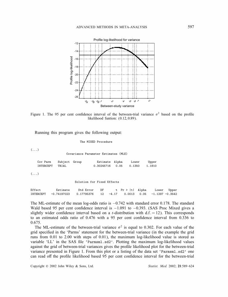
Figure 1. The 95 per cent con?dence interval of the between-trial variance �2 based on the pro?lelikelihood funtion: (0:12; 0:89).

Running this program gives the following output:

The MIXED Procedure

(...)Covariance Parameter Estimates (MLE)

Cov Parm Subject Group Estimate Alpha Lower UpperINTERCEPT TRIAL 0.30245716 0.05 0.1350 1.1810

(...)


Effect Estimate Std Error DF t Pr > |t| Alpha Lower UpperINTERCEPT -0.74197023 0.17795376 12 -4.17 0.0013 0.05 -1.1297 -0.3542

The ML-estimate of the mean log-odds ratio is −0:742 with standard error 0.178. The standardWald based 95 per cent con?dence interval is −1:091 to −0:393. (SAS Proc Mixed gives aslightly wider con?dence interval based on a t-distribution with d:f :=12). This correspondsto an estimated odds ratio of 0.476 with a 95 per cent con?dence interval from 0.336 to0.675.The ML-estimate of the between-trial variance �2 is equal to 0.302. For each value of the

grid speci?ed in the ‘Parms’ statement for the between-trial variance (in the example the gridruns from 0.01 to 2.00 with steps of 0.01), the maximum log-likelihood value is stored asvariable ‘LL’ in the SAS ?le ‘Parmsml.sd2’. Plotting the maximum log-likelihood valuesagainst the grid of between-trial variances gives the pro?le likelihood plot for the between-trialvariance presented in Figure 1. From this plot or a listing of the data set ‘Parmsml.sd2’ onecan read o< the pro?le likelihood based 95 per cent con?dence interval for the between-trial



Profile log-likelihood for mean

mean.40.0-.4-.8-1.2-1.6-2.0

prof

ile lo

g-lik

elih

ood

-13

-14

-15

-16

-17

-18

-19

-20

-21

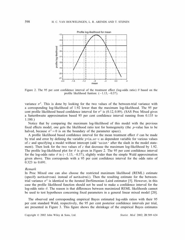
Figure 2. The 95 per cent con?dence interval of the treatment e<ect (log-odds ratio) � based on thepro?le likelihood funtion: (−1:13;−0:37).

variance �2. This is done by looking for the two values of the between-trial variance witha corresponding log-likelihood of 1.92 lower than the maximum log-likelihood. The 95 percent pro?le likelihood based con?dence interval for �2 is (0.12, 0.89). (SAS Proc Mixed givesa Satterthwaite approximation based 95 per cent con?dence interval running from 0.135 to1.180.)Notice that by comparing the maximum log-likelihood of this model with the previous

?xed e<ects model, one gets the likelihood ratio test for homogeneity (the p-value has to behalved, because �2 = 0 is on the boundary of the parameter space).A pro?le likelihood based con?dence interval for the mean treatment e<ect # can be made

by trial and error by de?ning the variable y=ln or-c as dependent variable for various valuesof c and specifying a model without intercept (add ‘noint’ after the slash in the model state-ment). Then look for the two values of c that decrease the maximum log-likelihood by 1.92.The pro?le log-likelihood plot for # is given in Figure 2. The 95 per cent con?dence intervalfor the log-odds ratio # is (−1:13;−0:37), slightly wider than the simple Wald approximationgiven above. This corresponds with a 95 per cent con?dence interval for the odds ratio of0.323 to 0.691.

RemarkIn Proc Mixed one can also choose the restricted maximum likelihood (REML) estimate(specify method=reml instead of method=ml). Then the resulting estimate for the between-trial variance �2 is identical to the iterated DerSimonian–Laird estimator [5]. However, in thiscase the pro?le likelihood function should not be used to make a con?dence interval for thelog-odds ratio #. The reason is that di<erences between maximized REML likelihoods cannotbe used to test hypotheses concerning ?xed parameters in a general linear mixed model [20].

The observed and corresponding empirical Bayes estimated log-odds ratios with their 95per cent standard Wald, respectively, the 95 per cent posterior con?dence intervals per trial,are presented in Figure 3. This ?gure shows the shrinkage of the empirical Bayes estimates



TR

IAL

1 (n= 262)

2 (n= 609)

3 (n= 451)

4 (n= 26,465)

5 (n= 10,877)

6 (n= 2,992)

7 (n= 3,174)

8 (n=176,782)

9 (n= 14,776)

10 (n= 3,381)

11 (n= 77,972)

12 (n= 4,839)

13 (n= 34,767)

LOG ODDS RATIO

3210-1-2-3

95% Confidence interval:

95% Prediction interval:

� = -0.742, 95% Conf. Int.= (-1.091 ; -0.393)

� = -0.742, 95% Pred. Int. = (-1.820 ; 0.336)

ˆ

ˆ

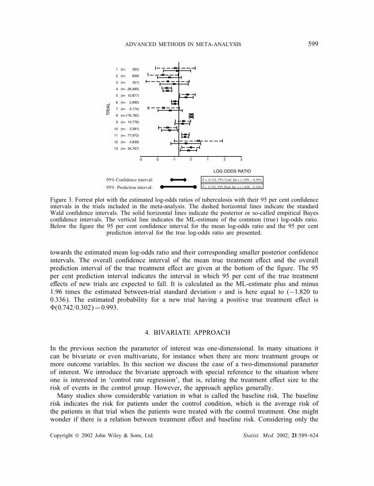
Figure 3. Forrest plot with the estimated log-odds ratios of tuberculosis with their 95 per cent con?denceintervals in the trials included in the meta-analysis. The dashed horizontal lines indicate the standardWald con?dence intervals. The solid horizontal lines indicate the posterior or so-called empirical Bayescon?dence intervals. The vertical line indicates the ML-estimate of the common (true) log-odds ratio.Below the ?gure the 95 per cent con?dence interval for the mean log-odds ratio and the 95 per cent

prediction interval for the true log-odds ratio are presented.

towards the estimated mean log-odds ratio and their corresponding smaller posterior con?denceintervals. The overall con?dence interval of the mean true treatment e<ect and the overallprediction interval of the true treatment e<ect are given at the bottom of the ?gure. The 95per cent prediction interval indicates the interval in which 95 per cent of the true treatmente<ects of new trials are expected to fall. It is calculated as the ML-estimate plus and minus1.96 times the estimated between-trial standard deviation s and is here equal to (−1:820 to0.336). The estimated probability for a new trial having a positive true treatment e<ect isQ(0:742=0:302)=0:993.

4. BIVARIATE APPROACH

In the previous section the parameter of interest was one-dimensional. In many situations itcan be bivariate or even multivariate, for instance when there are more treatment groups ormore outcome variables. In this section we discuss the case of a two-dimensional parameterof interest. We introduce the bivariate approach with special reference to the situation whereone is interested in ‘control rate regression’, that is, relating the treatment e<ect size to therisk of events in the control group. However, the approach applies generally.Many studies show considerable variation in what is called the baseline risk. The baseline

risk indicates the risk for patients under the control condition, which is the average risk ofthe patients in that trial when the patients were treated with the control treatment. One mightwonder if there is a relation between treatment e<ect and baseline risk. Considering only the



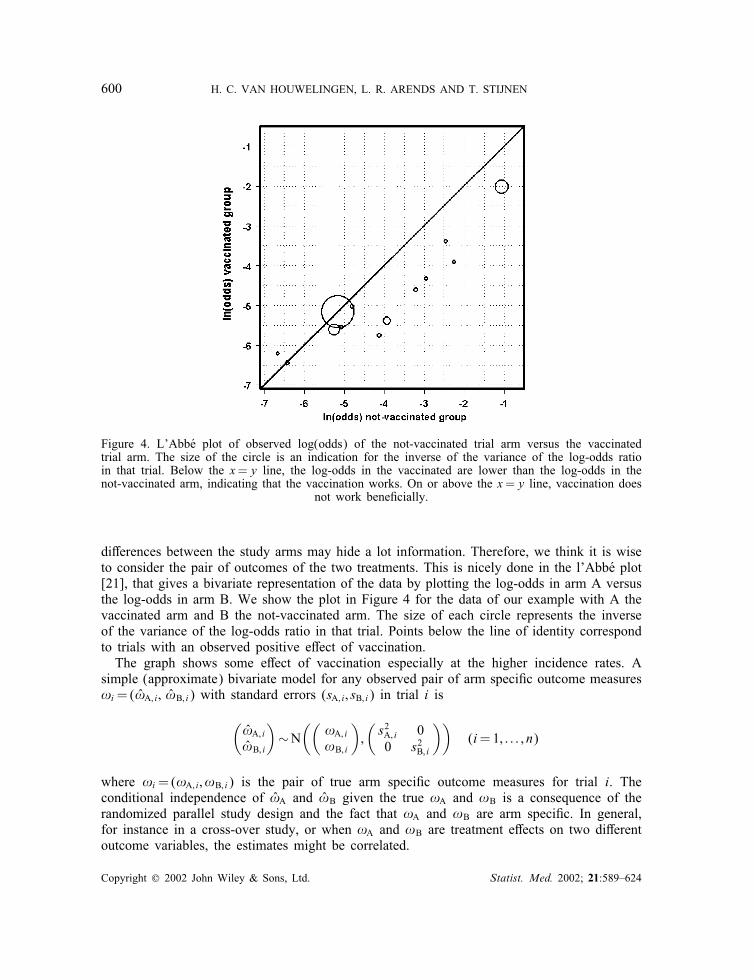
Figure 4. L’AbbUe plot of observed log(odds) of the not-vaccinated trial arm versus the vaccinatedtrial arm. The size of the circle is an indication for the inverse of the variance of the log-odds ratioin that trial. Below the x=y line, the log-odds in the vaccinated are lower than the log-odds in thenot-vaccinated arm, indicating that the vaccination works. On or above the x=y line, vaccination does

not work bene?cially.

di<erences between the study arms may hide a lot information. Therefore, we think it is wiseto consider the pair of outcomes of the two treatments. This is nicely done in the l’AbbUe plot[21], that gives a bivariate representation of the data by plotting the log-odds in arm A versusthe log-odds in arm B. We show the plot in Figure 4 for the data of our example with A thevaccinated arm and B the not-vaccinated arm. The size of each circle represents the inverseof the variance of the log-odds ratio in that trial. Points below the line of identity correspondto trials with an observed positive e<ect of vaccination.The graph shows some e<ect of vaccination especially at the higher incidence rates. A

simple (approximate) bivariate model for any observed pair of arm speci?c outcome measures!i=(!̂A; i ; !̂B; i) with standard errors (sA; i ; sB; i) in trial i is

(!̂A; i!̂B; i

)∼N

((!A; i!B; i

);(s2A; i 00 s2B; i

))(i=1; : : : ; n)

where !i=(!A; i ; !B; i) is the pair of true arm speci?c outcome measures for trial i. Theconditional independence of !̂A and !̂B given the true !A and !B is a consequence of therandomized parallel study design and the fact that !A and !B are arm speci?c. In general,for instance in a cross-over study, or when !A and !B are treatment e<ects on two di<erentoutcome variables, the estimates might be correlated.



The mixed model approach assumes the pair (!A; i ; !B; i) to follow a bivariate normal dis-tribution, where, analogous to the univariate random e<ects model of Section 3, the trueoutcome measures for both arms in the trials are normally distributed around some commonmean treatment-arm outcome measure with a between-trial covariance matrix V:(

!A; i

!B; i

)∼N

((!A!B

);V

)with V=

(VAA VABVAB VBB

)

VAA and VBB describe the variability among trials in true risk under the vaccination andcontrol condition, respectively. VAB is the covariance between the true risk in the vaccinationand control group.The resulting marginal model is

(!̂A; i!̂B; i

)∼N

((!A

!B

);V+ Ci

)

with Ci the diagonal matrix with the s2i ’s.Maximum likelihood estimation for this model can be quite easily carried out by a self-

made program based on the EM algorithm as described in reference [1], but more practicallyconvenient is to use appropriate mixed model software from statistical packages, such as theSAS procedure Proc Mixed.Once the model is ?tted, the following derived quantities are of interest:

(i) The mean di<erence (!A −!B) and its standard error

√{(var(!A) + var(!B)− 2 cov(!A; !B))}

(ii) The population variance of the di<erence var(!A −!B)=VAA + VBB − 2VAB.(iii) The shape of the bivariate relation between the (true) !A and !B. That can be

described by ellipses of equal density or by the regression lines of !A on !B and ofthe !B on !A. These lines can be obtained from classical bivariate normal theory.For example, the regression line of !A on !B has slope =VAB=VBB and residualvariance VAA − V2AB=VBB. The regression of the di<erence (!A − !B) on either !Aor !B can be derived similarly. At the end of this section we come back to theusefulness of these regression lines.

The standard errors of the regression slopes can be calculated from the covariance matrix ofthe estimated covariance parameters by the delta method or by Fieller’s method [22].

4.1. Example (continued): bivariate random e1ects model

As an example we carry out a bivariate meta-analysis with !A and !B the log-odds oftuberculosis in the vaccinated and the not-vaccinated control arm, respectively. To execute abivariate analysis in the SAS procedure Proc Mixed, we have to change the structure of thedata set. Each treatment arm of a trial becomes a row in the data set, resulting in twice asmany rows as in the original data set. The dependent variable is now the estimated log-odds



in a treatment arm instead of the log-odds ratio. The new data set is called BCGdata2.sd2 andthe observed log-odds is called lno. The standard error of the observed log-odds, estimatedby taking the square root of minus the inverse of the second derivative of the log-likelihood,is equal to

√(1x +

1n−x

), where n is the sample size of a treatment arm and x is the number

of tuberculosis cases in a treatment arm. These standard errors are also stored in the SASdata set covvars2.sd2.The bivariate random e<ects analysis can be carried out by running the SAS commands

given below. In the data step, the new data set BCGdata2.sd2 is made out of the data setBCGdata2.sd2, and the covariates are de?ned on trial arm level. The variable exp is 1 for thevaccinated (experimental) arms and 0 for the not-vaccinated (control) arms. The variable conis de?ned analogously with experimental and control reversed. The variable arm identi?es the26 unique treatment arms from the 13 studies (here from 1 to 26); latcon, latexp, yearconand yearexp are covariates to be used later. For numerical reasons we centralized the fourvariables latcon, latexp, yearcon and yearexp by substracting the mean.

# THE DATA STEP (BIVARIATE ANALYSIS)

data bcgdata2;set bcg_data;treat=1; lno=log(vd/vwd); var=1/vd+1/vwd; n=vd+vwd; output;treat=0; lno=log(nvd/nvwd); var=1/nvd+1/nvwd; n=nvd+nvwd; output;keep trial lno var n treat latitude--alloc;run;data bcgdata2;set bcgdata2;arm=_n_; exp=(treat=1); con=(treat=0);latcon=(treat=0)*(latitude-33); latexp=(treat=1)*(latitude-33);yearcon=(treat=0)*(year-66); yearexp=(treat=1)*(year-66);proc print noobs;run;

Running these SAS commands gives the following output:

LA Y YT L L E E

T I A T A A A AR T Y L R T T R RI U E L E L V A E C C E C EA D A O A N A R X O O X O XL E R C T O R M P N N P N P

1 44 48 1 1 -3.39283 0.25840 1 1 0 0 11 0 -181 44 48 1 0 -2.45413 0.09872 2 0 1 11 0 -18 02 55 49 1 1 -3.91202 0.17000 3 1 0 0 22 0 -172 55 49 1 0 -2.24583 0.03813 4 0 1 22 0 -17 03 42 60 1 1 -4.33073 0.33772 5 1 0 0 9 0 -63 42 60 1 0 -2.94444 0.09569 6 0 1 9 0 -6 04 52 77 1 1 -5.38597 0.01620 7 1 0 0 19 0 114 52 77 1 0 -3.92953 0.00411 8 0 1 19 0 11 0



5 13 73 2 1 -5.02786 0.03050 9 1 0 0 -20 0 75 13 73 2 0 -4.80872 0.02145 10 0 1 -20 0 7 06 44 53 2 1 -2.02302 0.00629 11 1 0 0 11 0 -136 44 53 2 0 -1.06490 0.00361 12 0 1 11 0 -13 07 19 73 1 1 -5.75930 0.12539 13 1 0 0 -14 0 77 19 73 1 0 -4.12552 0.10162 14 0 1 -14 0 7 08 13 80 1 1 -5.15924 0.00199 15 1 0 0 -20 0 148 13 80 1 0 -5.17126 0.00202 16 0 1 -20 0 14 09 27 68 1 1 -5.55135 0.03462 17 1 0 0 -6 0 29 27 68 1 0 -5.07961 0.02236 18 0 1 -6 0 2 0

10 42 61 3 1 -4.60458 0.05941 19 1 0 0 9 0 -510 42 61 3 0 -3.20337 0.01601 20 0 1 9 0 -5 011 18 74 3 1 -5.60295 0.00540 21 1 0 0 -15 0 811 18 74 3 0 -5.26210 0.00713 22 0 1 -15 0 8 012 33 69 3 1 -6.21180 0.20040 23 1 0 0 0 0 312 33 69 3 0 -6.65844 0.33376 24 0 1 0 0 3 013 33 76 3 1 -6.43840 0.03710 25 1 0 0 0 0 1013 33 76 3 0 -6.42106 0.03454 26 0 1 0 0 10 0

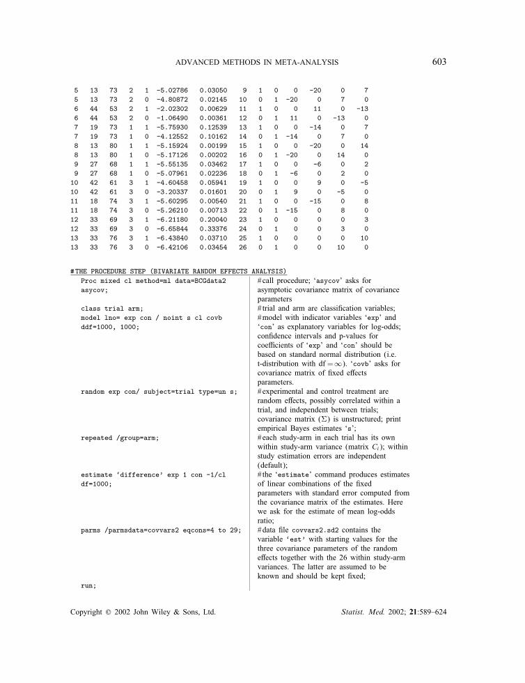
#THE PROCEDURE STEP (BIVARIATE RANDOM EFFECTS ANALYSIS)Proc mixed cl method=ml data=BCGdata2 #call procedure; ‘asycov’ asks forasycov; asymptotic covariance matrix of covariance

parametersclass trial arm; # trial and arm are classi?cation variables;model lno= exp con / noint s cl covb #model with indicator variables ‘exp’ andddf=1000, 1000; ‘con’ as explanatory variables for log-odds;

con?dence intervals and p-values forcoe=cients of ‘exp’ and ‘con’ should bebased on standard normal distribution (i.e.t-distribution with df =∞). ‘covb’ asks forcovariance matrix of ?xed e<ectsparameters.

random exp con/ subject=trial type=un s; #experimental and control treatment arerandom e<ects, possibly correlated within atrial, and independent between trials;covariance matrix (V) is unstructured; printempirical Bayes estimates ‘s’;

repeated /group=arm; #each study-arm in each trial has its ownwithin study-arm variance (matrix Ci); withinstudy estimation errors are independent(default);

estimate ‘difference’ exp 1 con -1/cl # the ‘estimate’ command produces estimatesdf=1000; of linear combinations of the ?xed

parameters with standard error computed fromthe covariance matrix of the estimates. Herewe ask for the estimate of mean log-oddsratio;

parms /parmsdata=covvars2 eqcons=4 to 29; #data ?le covvars2.sd2 contains thevariable ‘est’ with starting values for thethree covariance parameters of the randome<ects together with the 26 within study-armvariances. The latter are assumed to beknown and should be kept ?xed;

run;



Running this program gives the following output:

The MIXED Procedure


Cov Parm Subject Group Estimate Alpha Lower UpperUN(1,1) TRIAL 1.43137384 0.05 0.7369 3.8894UN(2,1) TRIAL 1.75732532 0.05 0.3378 3.1768UN(2,2) TRIAL 2.40732608 0.05 1.2486 6.4330

(...)


Effect Estimate Std Error DF t Pr > |t| Alpha Lower UpperEXP -4.83374538 0.33961722 1000 -14.23 0.0001 0.05 -5.5002 -4.1673CON -4.09597366 0.43469692 1000 -9.42 0.0001 0.05 -4.9490 -3.2430

Covariance Matrix for Fixed Effects

Effect Row COL1 COL2EXP 1 0.11533985 0.13599767CON 2 0.13599767 0.18896142

(...)ESTIMATE Statement Results

Parameter Estimate Std Error DF t Pr > |t| Alpha Lower Upperdifference -0.73777172 0.17973848 1000 -4.10 0.0001 0.05 -1.0905 -0.3851

The ?xed parameter estimates !̂=(!̂A; !̂B)= (−4:834;−4:096) represent the estimated meanlog-odds in the vaccinated and non-vaccinated group, respectively. The between-trial estimatedvariance of the log-odds is V̂AA =1:431 in the vaccinated groups and V̂BB =2:407 in the not-vaccinated groups. The between-trial covariance is estimated to be V̂AB =1:757. Thus, the esti-mated correlation between the true vaccinated and true control log-odds is V̂AB=(

√V̂AA ·√V̂BB)

=0:947. The estimated covariance matrix for the ML-estimates !̂B and !̂A is(var(!̂A) cov(!̂A; !̂B)

cov(!̂B; !̂A) var(!̂B)

)=(0:115 0:1360:136 0:189

)

The estimated mean vaccination e<ect, measured as the log-odds ratio, is equal to (!̂A −!̂B)= (−4:834−(−4:096))=−0:738. The standard error of the mean vaccination e<ect is equalto

√{var(!̂A) + var(!̂B)− 2 cov(!̂A; !̂B)}=√(0:115 + 0:189− 2 · 0:136)=0:180, almost

identical to the result of the univariate mixed model. This corresponds to an estimated oddsratio of exp(−0:738)=0:478 with a 95 per cent con?dence interval equal to (0:336; 0:680),again strongly suggesting an average bene?cial vaccination e<ect. The slope of the regressionline to predict the log-odds in the vaccinated group from the log-odds in the not-vaccinated



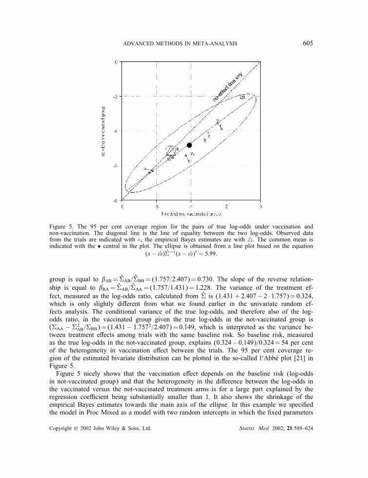
Figure 5. The 95 per cent coverage region for the pairs of true log-odds under vaccination andnon-vaccination. The diagonal line is the line of equality between the two log-odds. Observed datafrom the trials are indicated with ◦, the empirical Bayes estimates are with �. The common mean isindicated with the • central in the plot. The ellipse is obtained from a line plot based on the equation

(x − !̂)V̂−1(x − !̂)′ = 5:99.

group is equal to AB = V̂AB=V̂BB = (1:757=2:407)=0:730. The slope of the reverse relation-ship is equal to BA = V̂AB=V̂AA = (1:757=1:431)=1:228. The variance of the treatment ef-fect, measured as the log-odds ratio, calculated from V̂ is (1:431+ 2:407− 2 · 1:757)=0:324,which is only slightly di<erent from what we found earlier in the univariate random ef-fects analysis. The conditional variance of the true log-odds, and therefore also of the log-odds ratio, in the vaccinated group given the true log-odds in the not-vaccinated group is(VAA − V2

AB=VBB)= (1:431 − 1:7572=2:407)=0:149, which is interpreted as the variance be-tween treatment e<ects among trials with the same baseline risk. So baseline risk, measuredas the true log-odds in the not-vaccinated group, explains (0:324− 0:149)=0:324=54 per centof the heterogeneity in vaccination e<ect between the trials. The 95 per cent coverage re-gion of the estimated bivariate distribution can be plotted in the so-called l‘AbbUe plot [21] inFigure 5.Figure 5 nicely shows that the vaccination e<ect depends on the baseline risk (log-odds

in not-vaccinated group) and that the heterogeneity in the di<erence between the log-odds inthe vaccinated versus the not-vaccinated treatment arms is for a large part explained by theregression coe=cient being substantially smaller than 1. It also shows the shrinkage of theempirical Bayes estimates towards the main axis of the ellipse. In this example we speci?edthe model in Proc Mixed as a model with two random intercepts in which the ?xed parameters



correspond to !A and !B. An alternative would be to specify the model as a random-interceptrandom-slope model, in which the ?xed parameters correspond to !B and the mean treatmente<ect !A −!B. Then the SAS commands should be modi?ed as follows:

model lno=treat/s cl covb ddf=1000;random int treat/subject=trial type=un s;

Here int refers to a random trial speci?c intercept.

4.2. Relation between e1ect and baseline risk

The relation between treatment e<ect and baseline risk has been very much discussed in theliterature [6–9; 23–30]. There are two issues that complicate the matter:

1. The relation between ‘observed di<erence A−B’ and ‘observed baseline risk B’ is proneto spurious correlation, since the measurement error in the latter is negatively correlatedwith measurement error in the ?rst. It would be better to study B versus A or B − Aversus (A+B)=2.

2. Even in the regression of ‘observed risk in group A’ on ‘observed baseline risk in groupB’, which is not hampered by correlated measurement errors, the estimated slope isattenuated due to measurement error in the observed baseline risk [31].

For an extensive discussion of these problems see the article of Sharp et al. [32].In dealing with measurement error there are two approaches [31; 33]:

(i) The functional equation approach: true regressors as nuisance parameters.(ii) The structural equation approach: true regressors as random quantities with an un-

known distribution.

The usual likelihood theory is not guaranteed to work for the functional equation approachbecause of the large number of nuisance parameters. The estimators may be inconsistent orhave the wrong standard errors. The bivariate mixed model approach to meta-analysis used inthis paper is in the spirit of the structural approach. The likelihood method does work for thestructural equation approach, so in this respect our approach is safe. Of course, the question ofrobustness of the results against misspeci?cation of the mixing distribution is raised. However,Verbeke and Lesa<re [34] have shown that, in the general linear mixed model, the ?xede<ect parameters as well as the covariance parameters are still consistently estimated whenthe distribution of the random e<ects is misspeci?ed, so long as the covariance structure iscorrect. Thus our approach yields (asymptotically) unbiased estimates of slope and interceptof the regression line even if the normal distribution assumption is not ful?lled, although thestandard errors might be wrong. Verbeke and Lesa<re [34] give a general method for robustestimation of the standard errors.The mix of many ?xed and a few random e<ects as proposed by Thompson et al. [8] and

the models of Walter [9] and Cook and Walter [29] are more in the spirit of the functionalapproach. These methods are meant to impose no conditions on the distribution of the truebaseline risks. The method of Walter [9] was criticized by Bernsen et al. [35]. Sharp andThompson [30] use other arguments to show that Walter’s method is seriously Wawed. In aletter to the editor by Van Houwelingen and Senn [36] following the article of Thompson



et al. [8], Van Houwelingen and Senn [36] argue that putting Bayesian priors on all nuisanceparameters, as done by Thompson et al., does not help solving the inconsistency problem.This view is also supported in the chapter on Bayesian methods in the book of Carrollet al. [31]. It would be interesting to apply the ideas of Caroll et al. [31] in the setting ofmeta-analysis, but that is beyond the scope of this paper. Arends et al. [10] compare, in anumber of examples, the approach of Thompson et al. [8] with the method presented hereand the results were in line with the remarks of Van Houwelingen and Senn [36]. Sharp andThompson [30], comparing the di<erent approaches in a number of examples, remark thatwhether or not to assume a distribution for the true baseline risks remains a debatable issue.Arends et al. [10] also compared the approximate likelihood method as presented here with

an exact likelihood approach where the parameters are estimated in a Bayesian manner withvague priors and found no relevant di<erences.

5. META-REGRESSION

In case of substantial heterogeneity between the studies, it is the statistician’s duty to explorepossible causes of the heterogeneity [15; 37–39]. In the context of meta-analysis that canbe done by covariates on the study level that could ‘explain’ the di<erences between thestudies. The term meta-regression to describe such analysis goes back to papers by Bashoreet al. [40], Jones [41], Greenland [42] and Berlin and Antman [37]. We consider only analysesat the aggregated meta-analytic level. Aggregated information (mean age, percentage males)can describe the di<erences between studies. We will not go into covariates on the individuallevel. If such information exists, the data should be analysed on the individual patient level byhierarchical models. That is possible and a sensible thing to do, but beyond the scope of thispaper. We will also not consider covariates on the study arm level. That can be relevant in non-balanced observational studies. Such covariates could both correct the treatment e<ect itself incase of confounding as well as explain existing heterogeneity between studies. Although themethods presented in this paper might be applied straightforwardly, we will restrict attentionto balanced studies in which no systematic di<erence between the study arms is expected.Since the number of studies in a meta-analysis is usually quite small, there is a great danger

of over?tting. The rule of thumb of one explanatory variable for each 5 (10) ‘cases’ leavesonly room for a few explanatory variables in a meta-regression. In the example we have threecovariates available: latitude; year of study, and method of treatment allocation. Details aregiven in Table I.In the previous section we have seen that heterogeneity between studies can be partly

explained by di<erences in baseline risk. Thus, it is also important to investigate whethercovariates on the study level are associated with the baseline risk. That asks for a trulymultivariate regression with a two-dimensional outcome, but we will start with the simplerregression for the one-dimensional treatment e<ect di<erence measure.

5.1. Regression for di1erence measure

Let Xi stand for the (row)vector of covariates of study i including the constant term. Meta-regression relates the true di<erence #i to the ‘predictor’ Xi . This relation cannot be expectedto be perfect; there might be some residual heterogeneity that could be modelled by a normal



distribution once again, that is #i ∼ N(Xi ; �2). Taking into account the imprecision of theobserved di<erence measure #̂i we get the marginal approximate model

#̂i ∼ N(Xi ; �2 + s2i )

This model could be ?tted by iteratively reweighted least squares, where a new estimate of�2 is used in each iteration step or by full maximum likelihood with appropriate software. Inthe following we will describe how the model can be ?tted by SAS.

5.2. Example (continued)

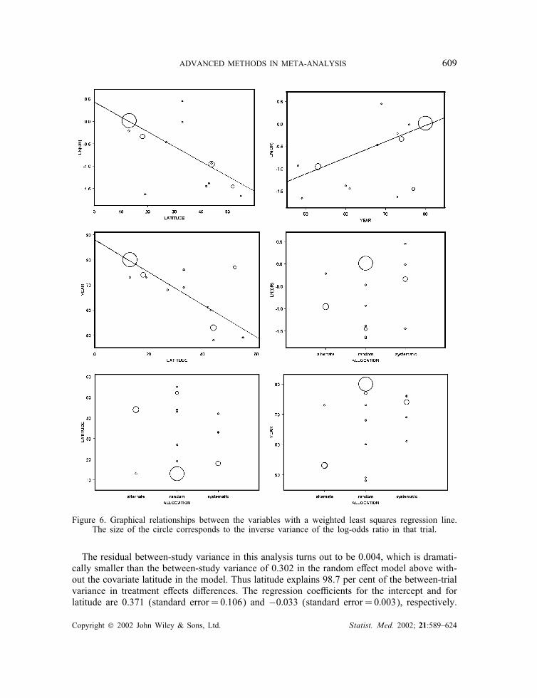
A graphical presentation of the data is given in Figure 6. Latitude and year of publicationboth seem to be associated with the log-odds ratio, while latitude and year are also correlated.Furthermore, at ?rst sight, the three forms of allocation seem to have little di<erent averagetreatment e<ects.

5.2.1. Regression on latitude. The regression analysis for the log-odds ratio on latitude canbe carried out by running the following mixed model in SAS:

Proc mixed cl method=ml #call procedure;data=BCG data;class trial; # trial is classi?cation variable;model ln or=latitude / s cl covb; # latitude is only predictor variable;random int/ subject=trial s; #random trial e<ect;repeated /group=trial; #each trial has its own within study

variances;parms /parmsdata=covvars3 eqcons=2 to #data set covvars3 contains a starting value14; for between study variance and 13 within

study variances which should be kept ?xed;run;

Running this program gives the following output:The MIXED Procedure


Cov Parm Subject Group Estimate Alpha Lower UpperINTERCEPT TRIAL 0.00399452 0.05 0.0004 1.616E29

(...)


Effect Estimate Std Error DF t Pr > |t| Alpha Lower UpperINTERCEPT 0.37108745 0.10596655 11 3.50 0.0050 0.05 0.1379 0.6043LATITUDE -0.03272329 0.00337134 0 -9.71 . 0.05 . .


Effect Row COL1 COL2INTERCEPT 1 0.01122891 -0.00031190LATITUDE 2 -0.00031190 0.00001137



Figure 6. Graphical relationships between the variables with a weighted least squares regression line.The size of the circle corresponds to the inverse variance of the log-odds ratio in that trial.

The residual between-study variance in this analysis turns out to be 0.004, which is dramati-cally smaller than the between-study variance of 0.302 in the random e<ect model above with-out the covariate latitude in the model. Thus latitude explains 98.7 per cent of the between-trialvariance in treatment e<ects di<erences. The regression coe=cients for the intercept and forlatitude are 0.371 (standard error =0:106) and −0:033 (standard error =0:003), respectively.



The estimated correlation between these estimated regression coe=cients is−0:873.Just for comparison we give the results of an ordinary weighted linear regression. The

weights are equal to the inverse squared standard error of the log-odds ratio, instead ofthe correct weights equal to the inverse squared standard error of the log-odds ratio plus �̂2.The intercept was 0.395 (SE=0:124) and the slope −0:033 (SE=0:004). The results are onlyslightly di<erent, which is explained by the very small residual between-study variance.

5.2.2. Regression on year. Running the same model as above, only changing latitude intoyear, the residual between-study variance becomes 0.209. Thus year of publication explains30.8 per cent of the between-trial variance in treatment e<ects di<erences, much less than thevariance explained by the covariate latitude. The regression coe=cients for the intercept andfor year are −2:800 (standard error =1:031) and 0.030 (standard error =0:015), respectively.The estimated correlation between these estimated regression coe=cients is −0:989.Again, just for comparison, we also give the results of the ordinary weighted linear regres-

sion. The intercept was −2:842 (SE=0:876) and the slope 0.033 (SE=0:012). Like in theprevious example, the di<erences are relatively small.

5.2.3. Regression on allocation. Running the model with allocation as only (categorical)covariate (in the SAS commands, specify: class trial alloc;), gives a residual between-study variance equal to 0.281. This means that only 7 per cent of the between-trial variance inthe treatment e<ect di<erences is explained by the di<erent forms of allocation. The treatmente<ects (log-odds ratio) do not di<er signi?cantly between the trials with random, alternateand systematic allocation (p=0:396).

5.2.4. Regression on latitude and year. When both covariates latitude and year are put intothe model, the residual between-study variance becomes only 0.002, corresponding with anexplained variance of 99.3 per cent, only slightly more than by latitude alone. The regressioncoe=cients for the intercept, latitude and year are, respectively, 0.494 (standard error =0:529),−0:034 (standard error =0:004) and −0:001 (standard error =0:006).We conclude that latitude gives the best explanation of the di<erences in vaccination e<ect

between the trials, since it already explains 98 per cent of the variation. Since the residualvariance is so small, the regression equation in this example could have been obtained byordinary weighted linear regression under the assumption of homogeneity. In the originalmedical report [4] on this meta-analysis the authors mentioned the strong relationship betweentreatment e<ect and latitude as well. They speculated that the biological explanation mightbe the presence of non-tuberculous myobacteria in the population, which is associated withgeographical latitude.Goodness-of-?t of the model obtained above can be checked as in the weighted least squares

approach by individual standardization of the residuals (#̂i−Xi ̂)=√(�2+s2i ) and using standard

goodness-of-?t checks.In interpreting the results of meta-regression analysis, it should be kept in mind that this

is all completely observational. Clinical judgement is essential for correct understanding ofwhat is going on. Baseline risk may be an important confounder and we will study its e<ectbelow.



5.3. Bivariate regression

The basis of the model is the relation between the pair (!A; i ; !B; i), for example, (truelog-odds in vaccinated group, true log-odds in control group) and the covariate vector Xi.Since the covariate has inWuence on both components we have a truly multivariate regressionproblem in the classical sense that can be modelled as

(!A; i

!B; i

)∼N(BXi;V)

Here, the matrix B is a matrix of regression coe=cients: the ?rst row for the A-componentand the second row for the B-component. Taking into account the errors in the estimates weget the (approximate) model

(!̂A; i

!̂B; i

)∼N(BXi;V+ Ci)

Fitting this model to the data can again be done by a self-made program using the EMalgorithm or by programs such as SAS Proc Mixed. The hardest part is the interpretation ofthe model. We will discuss the interpretation for the example.So far we have shown for our leading example the univariate ?xed e<ects model, the uni-

variate random e<ect without covariates, the bivariate random e<ects model without covariatesand eventually the univariate random e<ects model with covariates. We end this section witha bivariate random e<ects model with covariates.

5.4. Example (continued): bivariate meta-analysis with covariates

To carry out the bivariate regression analyses in SAS Proc Mixed we again need the dataset BCGdata2.sd2 which was organized on treatment arm level. In this example we takelatitude as the covariate. The model can be ?tted using the SAS code given below, wherethe variables exp, con and arm have the same meaning as in the bivariate analysis abovewithout covariates. The variable latcon is for the not-vaccinated (control) groups equal tothe latitude value of the trial and zero for the vaccinated (experimental) groups. The variablelatexp, is de?ned analogously with vaccinated and non-vaccinated reversed.

Proc mixed cl method=ml data=BCGdata2; # call procedure;class trial arm; # trial and treatment arm are

de?ned as classi?cation variables;model lno= con exp latcon latexp/noint s cl #model with indicator variablesddf=1000,1000,1000,1000; ‘exp’ and ‘con’ together with

latitude as explanatory variablefor log-odds in both treatment groups;

random con exp / subject=trial type=fa0(2) s ; # control arm and experimentaltrial arm are speci?ed as randome<ects; covariance matrix isunstructured, parameterized asfactor analytic;

repeated /group=arm; #each study-arm in each trial hasits own within study-arm error variance;



parms /parmsdata=covvars4 eqcons=4 to 29; # in the data ?le covvars4 threestarting values are given for thebetween study covariance matrix,together with the 26 withinstudy-arm variances. The latterare assumed to be known and kept ?xed;

estimate ‘difference slopes’ latexp 1 latcon -1 #estimate of the di<erence in/cl df = 1000; slope between the vaccinated

and not-vaccinated groups;run;

RemarkIn the program above we speci?ed type=fa0(2) instead of type=un for V. If one choosesthe latter, the covariance matrix is parameterized as[

"1 "2"2 "3

]

and unfortunately the program does not converge if the estimated correlation is (very near to)1, as is the case here. If one chooses the former, the covariance matrix is parameterized as[

"211 "11"12

"11"12 "212 + "222

]

and the program converges even if the estimated correlation is 1, that is, if "22 = 0.

Running the program gives the following output:


Covariance Parameter Estimates (MLE)

Cov Parm Subject Group Estimate Alpha Lower UpperFA(1,1) TRIAL 1.08715174 0.05 0.7582 1.6896FA(2,1) TRIAL 1.10733154 0.05 0.6681 1.5466FA(2,2) TRIAL -0.00000000 . . .

(...)Solution for Fixed Effects

Effect Estimate Std Error DF t Pr > |t| Alpha Lower UpperCON -4.11736845 0.30605608 1000 -13.45 0.0001 0.05 -4.7180 -3.5168EXP -4.82570990 0.31287126 1000 -15.42 0.0001 0.05 -5.4397 -4.2118LATCON 0.07246261 0.02192060 1000 3.31 0.0010 0.05 0.0294 0.1155LATEXP 0.03913388 0.02239960 1000 1.75 0.0809 0.05 -0.0048 0.0831

ESTIMATE Statement Results

Parameter Estimate Std Error DF t Pr > |t| Alpha Lower Upper

difference slopes -0.03332874 0.00284902 1000 -11.70 0.0001 0.05 -0.0389 -0.0277

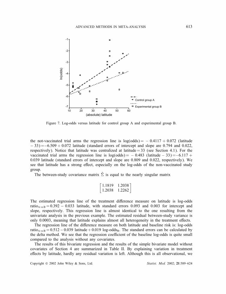
In Figure 7 the relationship between latitude and the log-odds of tuberculosis is presentedfor the vaccinated treatment arms A as well as for the non-vaccinated treatment arms B. For



(absolute) latitude605040302010

ln(o

dds)

-1

-2

-3

-4

-5

-6

-7

Control group A

Experimental group B

Figure 7. Log-odds versus latitude for control group A and experimental group B.

the not-vaccinated trial arms the regression line is log(odds)= − 0:4117 + 0:072 (latitude− 33)=−6:509 + 0:072 latitude (standard errors of intercept and slope are 0.794 and 0.022,respectively). Notice that latitude was centralized at latitude=33 (see Section 4.1). For thevaccinated trial arms the regression line is log(odds)= − 0:483 (latitude − 33)=−6:117 +0:039 latitude (standard errors of intercept and slope are 0.809 and 0.022, respectively). Wesee that latitude has a strong e<ect, especially on the log-odds of the non-vaccinated studygroup.The between-study covariance matrix V̂ is equal to the nearly singular matrix

[1:1819 1:20381:2038 1:2262

]

The estimated regression line of the treatment di<erence measure on latitude is log-oddsratioA vs B =0:392 − 0:033 latitude, with standard errors 0.093 and 0.003 for intercept andslope, respectively. This regression line is almost identical to the one resulting from theunivariate analysis in the previous example. The estimated residual between-study variance isonly 0.0003, meaning that latitude explains almost all heterogeneity in the treatment e<ects.The regression line of the di<erence measure on both latitude and baseline risk is: log-odds

ratioA vs B =0:512− 0:039 latitude+0:019 log-oddsB. The standard errors can be calculated bythe delta method. We see that the regression coe=cient of the baseline log-odds is quite smallcompared to the analysis without any covariates.The results of this bivariate regression and the results of the simple bivariate model without

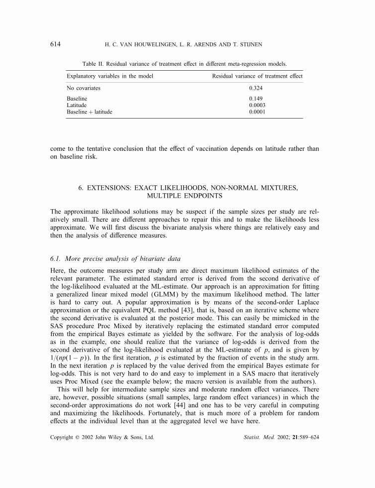
covariates of Section 4 are summarized in Table II. By explaining variation in treatmente<ects by latitude, hardly any residual variation is left. Although this is all observational, we



Table II. Residual variance of treatment e<ect in di<erent meta-regression models.

Explanatory variables in the model Residual variance of treatment e<ect

No covariates 0.324

Baseline 0.149Latitude 0.0003Baseline + latitude 0.0001

come to the tentative conclusion that the e<ect of vaccination depends on latitude rather thanon baseline risk.

6. EXTENSIONS: EXACT LIKELIHOODS, NON-NORMAL MIXTURES,MULTIPLE ENDPOINTS

The approximate likelihood solutions may be suspect if the sample sizes per study are rel-atively small. There are di<erent approaches to repair this and to make the likelihoods lessapproximate. We will ?rst discuss the bivariate analysis where things are relatively easy andthen the analysis of di<erence measures.

6.1. More precise analysis of bivariate data

Here, the outcome measures per study arm are direct maximum likelihood estimates of therelevant parameter. The estimated standard error is derived from the second derivative ofthe log-likelihood evaluated at the ML-estimate. Our approach is an approximation for ?ttinga generalized linear mixed model (GLMM) by the maximum likelihood method. The latteris hard to carry out. A popular approximation is by means of the second-order Laplaceapproximation or the equivalent PQL method [43], that is, based on an iterative scheme wherethe second derivative is evaluated at the posterior mode. This can easily be mimicked in theSAS procedure Proc Mixed by iteratively replacing the estimated standard error computedfrom the empirical Bayes estimate as yielded by the software. For the analysis of log-oddsas in the example, one should realize that the variance of log-odds is derived from thesecond derivative of the log-likelihood evaluated at the ML-estimate of p, and is given by1=(np(1−p)). In the ?rst iteration, p is estimated by the fraction of events in the study arm.In the next iteration p is replaced by the value derived from the empirical Bayes estimate forlog-odds. This is not very hard to do and easy to implement in a SAS macro that iterativelyuses Proc Mixed (see the example below; the macro version is available from the authors).This will help for intermediate sample sizes and moderate random e<ect variances. There

are, however, possible situations (small samples, large random e<ect variances) in which thesecond-order approximations do not work [44] and one has to be very careful in computingand maximizing the likelihoods. Fortunately, that is much more of a problem for randome<ects at the individual level than at the aggregated level we have here.



6.2. Example (continued)

After running the bivariate random e<ects model discussed in Section 4, the empirical Bayesestimates can be saved by adding the statement:

make ‘Predicted’ out = Pred;

in the Proc Mixed command and adding a ‘p’ after the slash in the model statement. In thisway the empirical Bayes estimates for log-odds are stored as variable PRED in the new SASdata ?le Pred.sd2. The within-trial variances in the next iteration of the SAS procedure ProcMixed are derived from these empirical Bayes estimates in the way we described above. Thethree starting values needed for the between-trial variance matrix are stored as variable estin the SAS ?le covvars5.sd2.Thus, after running the bivariate random e<ects model once and saving the empirical Bayes

estimates for log-odds, one can run the two data steps described below to compute the newestimates for the within-trial variances, use these within-trial variances in the next bivariatemixed model, save the new empirical Bayes estimates and repeat the whole loop. This iterativeprocess should be continued until the parameter estimates converge.

# DATA STEP TO COMBINE EMPIRICAL BAYES ESTIMATES AND ORIGINAL DATAFILE FROM SECTION 4 ANDTO CALCULATE THE NEW WITHIN-TRIAL VARIANCES;data Pred1;merge BCGdata2 Pred;pi=exp(_PRED_)/(1+exp(_PRED_));est=1/(n*pi*(1-pi));run;

# DATA STEP TO CREATE THE TOTAL DATAFILE THAT IS NEEDED IN THE PARMS-STATEMENT (BETWEEN-AND WITHIN-TRIAL VARIANCES);data Pred2;set covvars5 Pred1;run;

# PROCEDURE STEP TO RUN THE BIVARIATE RANDOM EFFECTS MODEL WITH NEW WITHIN-TRIALVARIANCES, BASED ON THE EMPIRICAL BAYES ESTIMATES.proc mixed cl method=ml data=BCGdata2 asycov;class trial arm;model lno= exp con / p noint s cl covb ddf=1000, 1000;random exp con/ subject=trial type=un s;repeated /group=arm subject=arm;estimate ‘difference’ exp 1 con -1 / cl df=1000;parms / parmsdata=Pred2 eqcons=4 to 29;run;

Running the data steps and the mixed model iteratively until convergence is reached givesthe following output:



Cov Parm Subject Group Estimate Alpha Lower UpperUN(1,1) TRIAL 1.43655989 0.05 0.7392 3.9084UN(2,1) TRIAL 1.76956270 0.05 0.3395 3.1996UN(2,2) TRIAL 2.43849037 0.05 1.2663 6.4991




Effect Estimate Std Error DF t Pr > |t| Alpha Lower Upper

EXP -4.84981269 0.34001654 1000 -14.26 0.0001 0.05 -5.5170 -4.1826CON -4.10942999 0.43736103 1000 -9.40 0.0001 0.05 -4.9677 -3.2512


Effect Row COL1 COL2EXP 1 0.11561125 0.13690215CON 2 0.13690215 0.19128467

ESTIMATE Statement Results

Parameter Estimate Std Error DF t Pr > |t| Alpha Lower Upperdifference -0.74038270 0.18191102 1000 -4.07 0.0001 0.05 -1.0974 -0.3834

The mean outcome measures (log-odds) for arms A and B are, respectively, −4:850(standard error =0:340) and 4.109 (standard error =0:437). The between-trial variance of thelog-odds in the vaccinated treatment arm A is V̂AA =1:437 and V̂BB =2:438 in the not-vaccinated arm B. The estimate of the between-trial covariance is equal to V̂AB =1:770. Theestimated mean vaccination e<ect in terms of the log-odds ratio is −0:740 (standard error =0:182). In this example, convergence was already reached after one or two iterations. The?nal estimates are very similar to the original bivariate random e<ects analysis we havediscussed in Section 4, where the mean outcome measures !̂A and !̂B were, respectively,−4:834 (SE=0:340) and −4:096 (SE=0:434). Of course, when the number of patients inthe trials were smaller, the bene?t and necessity of this method would be more substantial.Another possibility if the approximate likelihood solutions are suspect is to use the exact

likelihood, based on the binomial distribution of the number of events per treatment arm, andto estimate the parameters following a Bayesian approach with vague priors in combinationwith Markov chain Monte Carlo (MCMC) methods [45]. Arends et al. [10] give examplesof this approach. In their examples the di<erence with the approximate likelihood estimatesturned out to be very small.

6.3. More precise analysis of di1erence measures

The analysis of di<erence measures, that is, one summary measure per trial characterizingthe di<erence in e=cacy between treatments, is a bit more complicated because the baselinevalue is considered to be a nuisance parameter. Having this nuisance parameter can be avoidedand a lot of ‘exactness’ in the analysis can be gained by suitable conditioning on ancillarystatistics. In the case of binary outcomes one can condition on the marginals of the 2× 2tables and end up with the non-central hypergeometric distribution that only depends on thelog-odds ratio. Details are given in Van Houwelingen et al. [1].However, the hypergeometric distribution is far from easy to handle and it does not seem

very attractive to try to incorporate covariates in such an analysis as well. The bivariateanalysis is much easier to carry out at the price of the assumption that the baseline parameterfollows a normal distribution. However, that assumption can be relaxed as well and brings usto the next extension: the non-normal mixture.



6.4. Non-normal mixtures

The assumption of a normal distribution for the random e<ects might not be realistic. Tech-nically speaking it is not very hard to replace the normal mixture by a fully non-parametricmixture. As is shown by Laird [46], the non-parametric maximum likelihood estimator of themixing distribution is always a discrete mixture and can easily be estimated by means of theEM algorithm [47]. An alternative is to use the software C.A.MAN of BYohning et al. [48].However, just ?tting a completely non-parametric mixture is no good way of checking theplausibility of the normal mixture. The non-parametric estimates are always very discrete evenif the true mixture is normal. A better way is to see whether a mixture of two normals (withthe same variance) ?ts better than a single normal. This model can describe a very broadclass of distributions: unimodal as well as bimodal, symmetric as well as very skewed [19].Another way is to estimate the skewness of the mixture somehow and mistrust the normalityif the skewness is too big. It should be realized, however, that estimating mixtures is a kindof ill-posed problem and reliable estimates are hard to obtain [49]. To give an impression we?tted a non-parametric mixture with the homemade program based on the EM algorithm de-scribed in Van Houwelingen et al. [1] to the log-odds ratio of our example using approximatelikelihoods. The results were as follows:

atom probability−1:4577 0:3552−0:9678 0:1505−0:3296 0:29800:0023 0:1963

corresponding mean: −0:761corresponding variance: 0:349

The ?rst two moments agree quite well with the normal mixture. It is very hard to tell whetherthis four-point mixture gives any evidence against normality of the mixture. The bivariatenormal mixture of Section 4 is even harder to check. Non-parametric mixtures are hard to?t in two dimensions. An interesting question is whether the estimated regression slopes arerobust against non-normality. Arends et al. [10] modelled the baseline distribution with amixture of two normal distributions and found in all their examples a negligible di<erencewith modelling the baseline parameter with one normal distribution, indicating that the methodis robust indeed [10]. However, this was only based on three examples and we do not excludethe possibility that in some other data examples the regression slopes might be more di<erent.

6.5. Multiple outcomes

In a recent paper Berkey et al. [50] discussed a meta-analysis with multiple outcomes. Asimilar model was used in the context of meta-analysis of surrogate markers by Daniels andHughes [51] and discussed by Gail et al. [52]. In the simplest case of treatment di<erencemeasures for several outcomes, the situation is very similar to the bivariate analysis of Sec-tions 4 and 5. The model (

!A; i

!B; i

)∼N(BXi;V)



Table III.

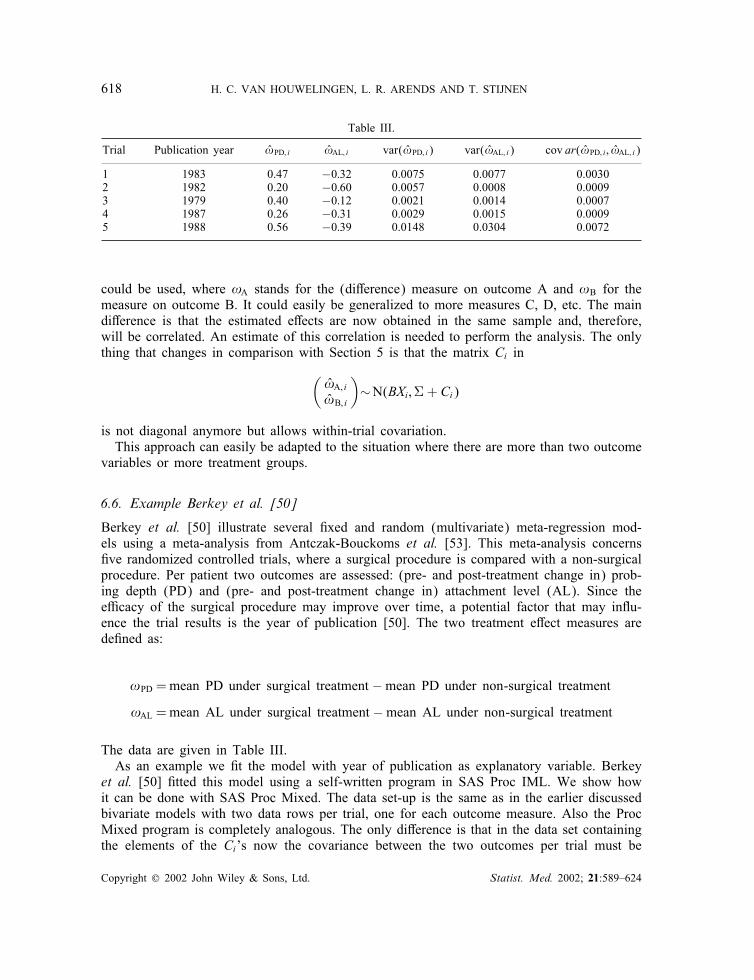
Trial Publication year !̂PD; i !̂AL; i var(!̂PD; i) var(!̂AL; i) cov ar(!̂PD; i ; !̂AL; i)

1 1983 0.47 −0:32 0.0075 0.0077 0.00302 1982 0.20 −0:60 0.0057 0.0008 0.00093 1979 0.40 −0:12 0.0021 0.0014 0.00074 1987 0.26 −0:31 0.0029 0.0015 0.00095 1988 0.56 −0:39 0.0148 0.0304 0.0072

could be used, where !A stands for the (di<erence) measure on outcome A and !B for themeasure on outcome B. It could easily be generalized to more measures C, D, etc. The maindi<erence is that the estimated e<ects are now obtained in the same sample and, therefore,will be correlated. An estimate of this correlation is needed to perform the analysis. The onlything that changes in comparison with Section 5 is that the matrix Ci in(

!̂A; i!̂B; i

)∼N(BXi;V+ Ci)

is not diagonal anymore but allows within-trial covariation.This approach can easily be adapted to the situation where there are more than two outcome

variables or more treatment groups.

6.6. Example Berkey et al. [50]

Berkey et al. [50] illustrate several ?xed and random (multivariate) meta-regression mod-els using a meta-analysis from Antczak-Bouckoms et al. [53]. This meta-analysis concerns?ve randomized controlled trials, where a surgical procedure is compared with a non-surgicalprocedure. Per patient two outcomes are assessed: (pre- and post-treatment change in) prob-ing depth (PD) and (pre- and post-treatment change in) attachment level (AL). Since thee=cacy of the surgical procedure may improve over time, a potential factor that may inWu-ence the trial results is the year of publication [50]. The two treatment e<ect measures arede?ned as:

!PD =mean PD under surgical treatment −mean PD under non-surgical treatment

!AL =mean AL under surgical treatment −mean AL under non-surgical treatment

The data are given in Table III.As an example we ?t the model with year of publication as explanatory variable. Berkey

et al. [50] ?tted this model using a self-written program in SAS Proc IML. We show howit can be done with SAS Proc Mixed. The data set-up is the same as in the earlier discussedbivariate models with two data rows per trial, one for each outcome measure. Also the ProcMixed program is completely analogous. The only di<erence is that in the data set containingthe elements of the Ci’s now the covariance between the two outcomes per trial must be



speci?ed as well. The SAS code is:

proc mixed cl method=ml data=berkey; #call procedure;class trial type; # trial and outcome type (PD ormodel outcome=pd al pdyear AL) are classi?cation variables;alyear/noint s cl; #model with indicator variables

‘pd’ and ‘al’ together withpublication year asexplanatory variable;

random pd al / subject=trial type=un s; #speci?cation of among-trialcovariance matrix forboth outcomes;

repeated type /subject=trial #speci?cation ofgroup=trial type=un; (non-diagonal) within-trial

covariance matrix;parms /parmsdata=covvars6 #covvars6 contains: 3 startingeqcons=4 to 18; values for the two between-trial

variances and covariance, 10within-trial variances (5 peroutcome measure) and 5covariances. The last 15parameters are assumed to beknown and must be kept ?xed.

run;

Part of the SAS Proc Mixed output is given below.



Cov Parm Subject Group Estimate Alpha Lower Upper

UN(1,1) TRIAL 0.00804054 0.05 0.0018 2.0771UN(2,1) TRIAL 0.00934132 0.05 -0.0113 0.0300UN(2,2) TRIAL 0.02501344 0.05 0.0092 0.1857

(...)Solution for Fixed Effects

Effect Estimate Std Error DF t Pr > |t| Alpha Lower UpperPD 0.34867848 0.05229098 3 6.67 0.0069 0.05 0.1823 0.5151AL -0.34379097 0.07912671 3 -4.34 0.0225 0.05 -0.5956 -0.0920PDYEAR 0.00097466 0.01543690 0 0.06 . 0.05 . .ALYEAR -0.01082781 0.02432860 0 -0.45 . 0.05 . .

The estimated model is

!PD = 0:34887 + 0:00097∗(year-1984)

!AL =−0:34595− 0:01082∗(year-1984)



The standard errors of the slopes are 0.0154 and 0.0243 for PD and AL, respectively. Theestimated among-trial covariance matrix is

V̂=(0:008 0:0090:009 0:025

)

The results are identical to those of Berkey et al. [50] with the random-e<ects multipleoutcomes that were estimated with the method named by Berkey as the multivariate maximumlikelihood (MML) method.

6.7. Other outcome measures

Our presentation concentrates on dichotomous outcomes. Much of it carries over to othere<ect measures that are measured on a di<erent scale. For instance, our methods apply ifthe outcome variable is continuous and an estimate of the average outcome and its standarderror is available in both treatment arms. However, in some cases only a relative e<ect isavailable, such as the standardized e<ect measure (di<erence in outcome=standard deviationof the measurements in the control group) which is popular in psychological studies. In thatcase only the one-dimensional analysis applies. A special case is survival analysis. The loghazard ratio in the Cox model cannot be written as the di<erence of two e<ect measures.However, some measure of baseline risk, for example, one-year survival rate in the controlarm, might be de?ned and the bivariate outcome analysis described above can be used toexplore the relation between treatment e<ect and baseline risk. A complicating factor is thatthe two measures are not independent any more. However, if an estimate of the correlationbetween the two measures is available, the method can be applied.

6.8. Other software

Although we illustrated all our examples with the SAS procedure Proc Mixed, most if not allanalyses could be carried out by other (general) statistical packages as well. A nice reviewof available software for meta-analysis has recently been written by Sutton et al. [54]. Anypackage like SPSS, SAS, S-plus and Stata that can perform a weighted linear regressionsu=ces to perform a standard ?xed e<ect meta-analysis or a ?xed e<ects meta-regression.For ?tting random e<ects models with approximate likelihood, a program for the general

linear mixed model (GLMM) is needed, which is available in many statistical packages.However, not all GLMM programs are appropriate. One essential requirement of the programis that one can ?x the within-trial variance in the model at arbitrary values per trial.In S-plus the function lme is used to ?t linear mixed e<ects models and all the analyses

carried out with Proc Mixed of SAS in our examples can also be carried out with lme fromS-plus. The ‘parms’ statement used by SAS to ?x the within-trial variances corresponds with‘varFixed’ in S-plus [55].Several Stata macros have been written which implement some of the discussed methods

[56; 57]. The Stata program meta of Sharp and Sterne [56] performs a standard ?xed andrandom e<ects meta-analysis without covariates. The Stata command metareg of Sharp [57]extends this to univariate meta-regression. We are not aware of Stata programs that are capableof ?tting bivariate meta-regression models, but of course one can do an univariate meta-regression on the log-odds ratios instead of a bivariate meta-regression on the log-odds of



the two treatment arms. However, such an analysis does not give any information about therelationship between the (true) log-odds of the two arms.Mlwin or MLn appears to be one of the most Wexible methods to ?t mixed-e<ect regression

models [54]. Although we do not have experience with this package, we assume that most ifnot all of the discussed models can be ?tted in it.Finally, in the free available Bayesian analysis software package BUGS, one can also

execute all approximate likelihood analyses that have been presented in this article. If vagueprior distributions are used, the results are very similar. With BUGS it is also possible to ?tthe models using the exact likelihood, based on the binomial distribution of the number ofevents in a treatment arm. The reader is referred to Arends et al. [10] for examples and therequired BUGS syntax.

7. BAYESIAN STATISTICS IN META-ANALYSIS

As we mentioned in Section 4, putting uninformative Bayesian priors on all individual nuisanceparameters as done in Thompson et al. [8], Daniels and Hughes [51], Smith et al. [58]and Sharp and Thompson [30] can lead to inconsistent results as the number of nuisanceparameters grows with the number of studies [36]. This observation does not imply that weoppose Bayesian methods. First of all, there is a lot of Bayesian Wavour to random e<ectsmeta-analysis. The mixing distribution can serve as a prior distribution in the analysis ofthe results of a new trial. However, the prior is estimated from the data and not obtainedby educated subjective guesses, that is why random e<ects meta-analysis can be seen as anexample of the empirical Bayes approach. For each study, the posterior distribution given theobserved value can be used to obtain empirical Bayes corrections.In this paper we describe estimating the mixing distribution by maximum likelihood. The

maximum likelihood method has two drawbacks. First, in complex problems, maximizing thelikelihood might become far from easy and quite time-consuming. Second, the constructionof con?dence intervals with the correct coverage probabilities can become problematic. Weproposed the pro?le likelihood approach in the simple setting of Section 3. For more complexproblems, the pro?le likelihood gets very hard to implement.When the maximum likelihood approach gets out of control (very long computing times,

non-convergence of the maximization procedure), it can be very pro?table to switch to aBayesian approach with vague priors on the parameters of the model in combination withMarkov chain Monte Carlo (MCMC) methods [45] that circumvent integration by replacing itby simulation. If one wants to use the MCMC technique in this context, the prior should be seton all parameters of the hierarchical model. Such a model could be described as a Bayesianhierarchical or Bayesian empirical Bayes model. For examples of this approach, see Arendset al. [10]. The di<erence with the approach of Thompson et al. [8; 30] is then that theyassume that the true baseline log-odds are a random sample of a fully speci?ed Wat normaldistribution (for example, N(0; 10)), while we assume that the true log-odds are sampled froma N(�; �) distribution with � and � parameters to be estimated, putting vague priors on them.So Thompson et al.’s model is a special case of our model. We prefer the parameters of thebaseline risks distribution to be determined by the data. For the examples discussed in thispaper, maximum likelihood was quite convenient in estimating the parameters of the modeland getting a rough impression of their precision. It su=ced for the global analysis described



here. If the model is used to predict outcomes of new studies, as in the surrogate marker settingof Daniels and Hughes [51], nominal coverage of the prediction intervals becomes importantand approximate methods can be misleading. MCMC can be very convenient, because theprediction problem can easily be embedded in the MCMC computations. An alternative isbootstrapping as described in Gail et al. [52].

8. CONCLUSIONS

We have shown that the general linear mixed model using an approximate likelihood approachis a very useful and convenient framework to model meta-analysis data. It can be used for thesimple meta-analysis up to complicated meta-analyses involving multivariate treatment e<ectmeasures and explanatory variables. Extension to multiple outcome variables and multipletreatment arms is very straightforward. Suitable software is widely available in statisticalpackages.

ACKNOWLEDGEMENTS

This paper is based on a course on meta-analysis given by Van Houwelingen and Stijnen at the ISCB inDundee in 1998. We thank the organizers for their stimulating invitation. We thankfully acknowledgethe help of Russ Wol?nger of SAS in ?nding the best Proc Mixed speci?cations for the bivariatemodels. We are very grateful to three reviewers for their detailed comments and valuable suggestions,which have led to considerable improvements of this paper.

REFERENCES

1. Van Houwelingen H, Zwinderman K, Stijnen T. A bivariate approach to meta-analysis. Statistics in Medicine1993; 12:2272–2284.

2. Berkey CS, Hoaglin DC, Mosteller F, Colditz GA. Random e<ects regression model for meta-analysis. Statisticsin Medicine 1995; 14:396–411.

3. Normand S-L. Meta-analysis: formulating, evaluating, combining and reporting. Statistics in Medicine 1999;18:321–359.

4. Colditz GA, Brewer FB, Berkey CS, Wilson EM, Burdick E, Fineberg HV, Mosteller F. E=cacy of BCGvaccine in the prevention of tuberculosis. Journal of the American Medical Association 1994; 271:698–702.

5. DerSimonian R, Laird N. Meta-analysis in clinical trials. Controlled Clinical Trials 1986; 7(3):177–188.6. Brand R, Kragt H. Importance of trends in the interpretation of an overall odds ratio in the meta-analysis ofclinical trials. Statistics in Medicine 1992; 11(16):2077–2082.

7. McIntosh MW. The population risk as an explanatory variable in research syntheses of clinical trials. Statisticsin Medicine 1996; 15:1713–1728.

8. Thompson SG, Smith TC, Sharp SJ. Investigating underlying risk as a source of heterogeneity in meta-analysis.Statistics in Medicine 1997; 16(23):2741–2758.

9. Walter SD. Variation in baseline risk as an explanation of heterogeneity in meta-analysis. Statistics in Medicine1997; 16:2883–2900.

10. Arends LR, Hoes AW, Lubsen J, Grobbee DE, Stijnen T. Baseline risk as predictor of treatment bene?t: threeclinical meta-re-analyses. Statistics in Medicine 2000; 19(24):3497–3518.

11. Fleiss JL. Analysis of data from multiclinic trials. Controlled Clinical Trials 1986; 7:267–275.12. Yusuf S, Peto R, Lewis J, Collins R, Sleight P. Beta blockade during and after myocardial infarction: an

overview of the randomised trials. Progress in Cardiovascular Diseases 1985; 27:335–371.13. Whitehead A, Whitehead J. A general parametric approach to the meta-analysis of clinical trials. Statistics in

Medicine 1991; 10:1665–1677.14. Hardy RJ, Thompson SG. A likelihood approach to meta-analysis with random e<ects. Statistics in Medicne

1996; 15:619–629.15. Greenland S. Quantitative methods in the review of epidemiologic literature. Epidemiologic Reviews 1987; 9:

1–30.



16. Newcombe RG. Improved con?dence intervals for the di<erence between binomial proportions based on paireddata. Statistics in Medicine 1998; 17:2635–2650.

17. Newcombe RG. Interval estimation for the di<erence between independent proportions: comparison of elevenmethods. Statistics in Medicine 1998; 17:873–890.

18. Brockwell SE, Gordon IR. A comparison of statistical methods for meta-analysis. Statistics in Medicine 2001;20:825–840.

19. Verbeke G. Linear mixed models for longitudinal data. In Linear Mixed Models in Practice, Verbeke G,Molenberghs G (eds). Springer-Verlag: New York, 1997; 63–153.

20. Roger JH, Kenward MG. Repeated measures using proc mixed instead of proc glm. In Proceedings of the FirstAnnual South-East SAS Users Group Conference. SAS Institute: Cary NC, 1993; 199–208.

21. L’AbbUe KA, Detsky AS. Meta-analysis in clinical research. Annals of Internal Medicine 1987; 107(2):224–233.

22. Armitage P, Berry G. Statistical Methods in Medical Research. Blackwell Scienti?c Publications: Oxford,1978.

23. Davey Smith G, Song F, Sheldon TA. Cholesterol lowering and mortality: the importance of considering initiallevel of risk. British Medical Journal 1993; 306(6889):1367–1373.

24. Senn S. Importance of trends in the interpretation of an overall odds ratio in the meta-analysis of clinical trials(letter). Statistics in Medicine 1994; 13(3):293–296.

25. Brand R. Importance of trends in the interpretation of an overall odds ratio in the meta-analysis of clinical trials(letter). Statistics in Medicine 1994; 13(3):293–296.

26. Hoes AW, Grobbee DE, Lubsen J. Does drug treatment improve survival? Reconciling the trials in mild-to-moderate hypertension. Journal of Hypertension 1995; 13(7):805–811.

27. Egger M, Smith GD. Risks and bene?ts of treating mild hypertension: a misleading meta-analysis? [comment].Journal of Hypertension 1995; 13(7):813–815.

28. Senn SJ. Relation between treatment bene?t and underlying risk in meta-analysis. British Medical Journal 1996;313:1550.

29. Cook RJ, Walter SD. A logistic model for trend in 2×2×K tables with applications to meta-analyses. Biometrics1997; 53(1):352–357.

30. Sharp SJ, Thompson SG. Analysing the relationship between treatment e<ect and underlying risk in meta-analysis: comparison and development of approaches. Statistics in Medicine 2000; 19:3251–3274.

31. Carroll RJ, Ruppert D, Stefanski LA. Measurement Error in Nonlinear Models. Chapman & Hall: London,1995.

32. Sharp SJ, Thompson SG, Altman DG. The relation between treatment bene?t and underlying risk in meta-analysis. British Medical Journal 1996; 313(7059):735–738.

33. Kendall MG, Stuart A. The Advanced Theory of Statistics. Volume II: Inference and Relationship. Gri=n:London, 1973.

34. Verbeke G, Lesa<re E. The e<ect of misspecifying the random e<ects distribution in linear models forlongitudinal data. Computational Statistics and Data Analysis 1997; 23:541–556.

35. Bernsen RMD, Tasche MJA, Nagelkerke NJD. Some notes on baseline risk and heterogeneity in meta-analysis.Statistics in Medicine 1999; 18(2):233–238.

36. Van Houwelingen HC, Senn S. Investigating underlying risk as a source of heterogeneity in meta-analysis(letter). Statistics in Medicine 1999; 18:107–113.

37. Berlin JA, Antman EM. Advantages and limitations of meta-analytic regressions of clinical trials data. OnlineJournal of Current Clinical Trials 1994; 134.

38. Thompson SG. Why sources of heterogeneity in meta-analysis should be investigated. British Medical Journal1994; 309(6965):1351–1355.

39. Thompson SG, Sharp SJ. Explaining hetergoneity in meta-anaysis: a comparison of methods. Statistics inMedicine 1999; 18:2693–2708.

40. Bashore TR, Osman A, He\ey EF. Mental slowing in elderly persons: a cognitive psychophysiological analysis.Psychology & Aging 1989; 4(2):235–244.

41. Jones DR. Meta-analysis of observational epidemiological studies: a review. Journal of the Royal Society ofMedicine 1992; 85(3):165–168.

42. Greenland S. A critical look at some popular meta-analytic methods. American Journal of Epidemiology 1994;140(3):290–296.

43. Platt RW, Leroux BG, Breslow N. Generalized linear mixed models for meta-analysis. Statistics in Medicine1999; 18:643–654.

44. Engel B. A simple illustration of the failure of PQL, IRREML and APHL as approximate ML methods formixed models for binary data. Biometrical Journal 1998; 40:141–154.

45. Gilks WR, Richardson S, Spiegelhalter DJ. Markov Chain Monte Carlo in Practice. Chapman & Hall: London,1996.

46. Laird NM. Nonparametric maximum likelihood estimation of a mixing distribution. Journal of the AmericanStatistical Association 1978; 73:805–811.



47. Dempster AP, Laird NM, Rubin DB. Maximum likelihood from incomplete data via the EM algorithm (withdiscussion). Journal of the Royal Statistical Society, Series B 1977; 39(1):1–38.

48. BYohning D, Schlattman P, Linsay B. Computer-assisted analysis of mixtures. Biometrics 1992; 48:283–304.49. Eilers PHC, Marx BD. Flexible smooting using B-splines and penalized likelihood. Statistical Science 1996;

11:89–121.50. Berkey CS, Hoaglin DC, Antczak-Bouckoms A, Mosteller F, Colditz GA. Meta-analysis of multiple outcomes

by regression with random e<ects. Statistics in Medicine 1998; 17:2537–2550.51. Daniels MJ, Hughes MD. Meta-analysis for the evaluation of potential surrogate markers. Statistics in Medicine

1997; 16:1965–1982.52. Gail MH, Pfei<er R, van Houwelingen HC, Carroll RJ. On meta-analytic assessment of surrogate outcomes.

Biostatistics 2000; 1(3):231–246.53. Antczak-Bouckoms A, Joshipura K, Burdick E, Tulloch JFC. Meta-analysis of surgical versus non-surgical

method of treatment for periodontal disease. Journal of Clinical Periodontology 1993; 20:259–268.54. Sutton AJ, Lambert PC, Hellmich M, Abrams KR, Jones DR. Meta-analysis in practice: a critical review of

available software. In Meta-Analysis in Medicine and Health Policy, Berry DA, Stangl DK (eds). MarcelDekker: New York, 2000.

55. Pinheiro JC, Bates DM. Mixed-e1ects Models in S and S-Plus. Springer-Verlag: Berlin, 2000.56. Sharp S, Sterne J. Meta-analysis. Stata Technical Bulletin 1997; 38(sbe 16):9–14.57. Sharp S. Meta-analysis regression. Stata Technical Bulletin 1998; 42(23):16–22.58. Smith TC, Spiegelhalter DJ, Thomas A. Bayesian approaches to random-e<ects meta-analysis: a comparative

study. Statistics in Medicine 1995; 14:2685–2699.


advanced methods in meta-analysis: multivariate approach and

Documents