ERNEST ORLANDO LAWRENCE

BERKELEY NATIONAL LABORATORY

Addressing Water Consumption of Evaporative Coolers with Greywater

Rashmi Sahai, Nihar Shah, Amol Phadke

Environmental Energy Technologies Division

International Energy Studies Group

July 1, 2012

This work was funded by the Bureau of Oceans and International Environmental and Scientific Affairs, U.S. Department of State, and administered by the U.S. Department of Energy in support of the Super-efficient Equipment and Appliance Deployment (SEAD) initiative through the U.S. Department of Energy under Contract No. DE-AC02-05CH11231

Disclaimer

This document was prepared as an account of work sponsored by the United States Government in support of the Super-efficient Equipment and Appliance Deployment (SEAD) initiative. While this document is believed to contain correct information, neither the United States Government nor any agencies thereof, SEAD participating Governments nor any agencies thereof, the SEAD Operating Agent, The Regents of the University of California, nor any of their employees, makes any warranty, express or implied, or assumes any legal responsibility for the accuracy, completeness, or usefulness of any information, apparatus, product, or process disclosed, or represents that its use would not infringe privately owned rights. Reference herein to any specific commercial product, process, or service by its trade name, trademark, manufacturer, or otherwise, does not necessarily constitute or imply its endorsement, recommendation, or favoring by the United States Government or any agency thereof, SEAD participating Governments or any agencies thereof, the SEAD Operating Agent, or The Regents of the University of California. The views and opinions of authors expressed herein do not necessarily state or reflect those of the United States Government or any agency thereof, SEAD participating Governments or any agencies thereof, the SEAD Operating Agent or The Regents of the University of California.

Ernest Orlando Lawrence Berkeley National Laboratory is an equal opportunity employer.

iii

Contents

List of Figures .......................................................................................................................................... iv List of Tables .............................................................................................................................................. v Abbreviations and Acronyms ............................................................................................................... vi Abstract ....................................................................................................................................................... 1 1. Introduction ......................................................................................................................................... 2 1.1. Background .................................................................................................................................................................. 2 1.2. The Technology ........................................................................................................................................................... 3 1.3. Purpose ......................................................................................................................................................................... 4 2. Global Deployment of Evaporative Cooling Technologies ....................................................... 5 2.1. Methods ........................................................................................................................................................................ 5 2.2. Results and Discussion ............................................................................................................................................... 5 3. Water Consumption of Evaporative Coolers ................................................................................ 7 3.1. Methods ........................................................................................................................................................................ 7 3.1.1. Calculating Cooling Load ........................................................................................................................................ 7 3.1.2. Water Consumption Due to Cooling .................................................................................................................... 9 3.1.3. Sensitivity Analysis ................................................................................................................................................... 9 3.1.4. Water Consumption due to Bleeding .................................................................................................................. 10 3.2. Results and Discussion ............................................................................................................................................. 11 3.2.1. Water Consumption of Evaporative Coolers .................................................................................................... 11 3.2.2. Sensitivity Analysis ................................................................................................................................................. 13 4. Greywater for Evaporative Cooling .............................................................................................. 14 4.1. Technical Feasibility. .................................................................................................................................................. 14 4.2 Cost Effectiveness ...................................................................................................................................................... 14 4.2.1. Methods ................................................................................................................................................................... 14 4.2.2. Discussion and Results .......................................................................................................................................... 17 5. Summary and Conclusions ............................................................................................................. 20 Acknowledgments .................................................................................................................................. 21 References................................................................................................................................................. 22 Appendix A. SEAD Countries .............................................................. Error! Bookmark not defined.

iv

List of Figures Figure 2-1. Geographic Suitability of Evaporative Cooling Technologies ................................................................ 6 Figure 3-1. Example of a Daily Temperature Profile Curve ....................................................................................... 8 Figure 3-2. Geographic Distribution of EC Water Consumption and Alkalinity Levels ..................................... 12 Figure 3-3. Results of Sensitivity Analysis - Variation in Water Consumption Range .......................................... 13 Figure 4-1. Total Life Cycle Costs of Various Cooling Technologies ...................................................................... 17 Figure 4-2. Life Cycle Costs Broken Down by Category ........................................................................................... 18

v

List of Tables

Table 2-1. Boundary Conditions used in EC Suitability Analysis ............................................................................... 5 Table 3-1. Equations Used to Calculate Cooling Load ................................................................................................. 8 Table 3-2. Variable Ranges for Sensitivity Analysis ................................................................................................. 10 Table 4-1. Upfront Cost and Characteristics of Technologies in the United States .............................................. 15 Table 4-2. Upfront Cost and Characteristics of Technologies in India ................................................................... 15 Table 4-3. City-Specific Inputs ........................................................................................................................................ 16

vi

Abbreviations and Acronyms

A area

ASHRAE American Society of Heating, Refrigeration and Air Conditioning Engineers

BTU British thermal units

°C degrees Celsius

CaCO3 eq. calcium carbonate equivalent

CFCs chlorofluorocarbons

CLF cooling load factor for glass

CLTD cooling load temperature difference

d day

DBT dry-bulb temperature

EC evaporative cooler

EER energy efficiency ratio

°F degrees Fahrenheit

ft.2 square feet

GW greywater

h hour of the day

hd household

HFCs hydroflorocarbons

hmax hour of day when tmax occurs

IR infiltration rate

kWh kilowatt-hours

L liters

LCCA life cycle cost analysis

LM latitude month correction

m2 square meters

M-cycle Maisotsenko Cycle

mg milligrams

MJ megajoules

vii

RAC room air conditioner

s seconds

SHGFmax maximum solar heat gain factor

tmax difference between 2% design DBT and indoor temperature

USD United States Dollars

U-value coefficient of transmission

W watts

w distance between hmax and h at the x-intercept

yr. years

1

Abstract

Evaporative coolers (ECs) provide significant gains in energy efficiency compared to vapor compression air conditioners, but simultaneously have significant onsite water demand. This can be a major barrier to deployment in areas of the world with hot and arid climates. To address this concern, this study determined where in the world evaporative cooling is suitable, the water consumption of ECs in these cities, and the potential that greywater can be used reduce the consumption of potable water in ECs. ECs covered 69% of the cities where room air conditioners are may be deployed, based on comfort conditions alone. The average water consumption due to ECs was found to be 400 L/household/day in the United States and Australia, with the potential for greywater to provide 50% this amount. In the rest of the world, the average water consumption was 250 L/household/day, with the potential for greywater to supply 80% of this amount. Home size was the main factor that contributed to this difference. In the Mediterranean, the Middle East, Northern India, and the Midwestern and Southwestern United States alkalinity levels are high and water used for bleeding will likely contribute significantly to EC water consumption.

Although technically feasible, upfront costs for household GW systems are currently high. In both developed and developing parts of the world, however, a direct EC and GW system is cost competitive with conventional vapor compression air conditioners. Moreover, in regions of the world that face problems of water scarcity the benefits can substantially outweigh the costs.

2

1. Introduction

1.1. Background

The use and ownership of room air conditioners (RACs) is increasing rapidly across the globe. Between 2010 and 2030, the developing world is predicted to increase its energy consumption from residential air conditioning by over 350% (McNeil & Letschert 2008) and the sales of RACs in Europe are anticipated to increase by 53% (Ecodesign 2008). This increase is driven by a worldwide trend towards higher income. The function between income and air conditioner ownership can be characterized by a sigmoidal curve. Because a RAC is a major luxury investment for most developing countries, average income must hit a certain threshold before RAC demand starts rising steeply. Empirical data suggests this threshold to be around an average annual per capita income of 3300 USD, which many developing countries recently surpassed. Only when saturation (which is unique to each climatic region) is reached, is demand anticipated to flatten out again (McNeil & Letschert 2006). The increased use and ownership of RACs is also driven by urbanization. With a migration towards cities, especially in developing countries, more people are exposed to the urban heat island effect. Temperatures in urban areas can be over 12 °C higher than the surrounding countryside (Rizwan et al. 2008). As a result, demand for air conditioning is also higher. In the process of cooling indoor temperatures, RACs produce a lot of waste heat that is ejected into the atmosphere and contributes to the urban heat island effect. Hence, there is a positive feedback loop that results – as the use of air conditioning increases, the outdoor temperature increases, causing air conditioning use to increase even more (Hsieh et al. 2007; Wen & Lian 2009). The expanding use and ownership of RACs presents both global and regional concerns. Globally, the emissions from electricity generation produced to power these air conditioners will contribute significantly to the rapidly growing stock of carbon in the atmosphere. This is also a positive feedback loop – emissions due to air conditioning increase the earth’s temperature, which will increase air conditioning use and generate more emissions into the atmosphere. On a regional scale, there is a growing contribution of air conditioning power load to the overall peak electricity system demand. Consequently, hot summer days have resulted in national power shortages (Lin & Rosenquist, 2008) and increased wholesale electricity prices. The problem is exacerbated by the fact that the efficiency of vapor compression air conditioners decreases as temperature increases, causing air conditioning load to be even higher on the hottest days of the year. To mitigate the impacts of growing AC demand, policy makers and utilities turn to increased efficiency as a negative-cost solution. In 2005, China implemented a new set of minimum efficiency standards for RACs, with a lowest allowable energy efficiency ratio (EER) of 2.5 watts/watt (W/W). By 2020, the cumulative reduction in CO2 emissions from this standard alone will add up to over 300 million tons of CO2, which is close to the total size of European commitment under the Kyoto regime (1997-2012) (Lin & Rosenquist 2008). These types of standards are a step in the right direction, however, they only address vapor compression air conditioners. They do not address evaporative cooling air conditioners (ECs), which easily have an EER of 20 W/W. Not only is their efficiency an order of magnitude greater than vapor compression coolers, evaporative coolers do not use refrigerants for cooling (which can contain CFCs and HFCs, ozone depleting substances and potent greenhouse gasses), and do not decrease their energy efficiency as temperature increases.

3

1.2. The Technology

There are four main types of evaporative cooling technologies: direct, indirect, indirect/direct, and Maisotsenko Cycle (M-Cycle). In a direct EC, outside air is drawn through wetted filter pads, where the hot, dry air is adiabatically cooled by the latent heat of evaporation. The dry-bulb temperature of the air leaving the wetted pads approaches the wet-bulb temperature of the ambient air. Since the supply air can never be colder than the wet-bulb temperature and is close to 100% relative humidity, direct ECs are most effective in dry climates (Saman, Bruno & Liu 2009).

In an indirect EC, cool air produced by direct evaporative cooling transfers conductive cooling across a heat exchanger to the supply air stream. Because the evaporatively-cooled (working) air stream never mixes with the supply air, the supply air becomes cooler without an increase in its humidity (Saman, Bruno & Liu 2009). In indirect/direct ECs, the first, indirect stage sensibly cools the primary air without increasing its moisture content. The air is then evaporatively-cooled further in the second, direct stage. The dry-bulb temperature of the supply air can be reduced to 6 °C or more below the wet-bulb temperature of the outside air without adding too much moisture (Saman, Bruno & Liu 2009). This extends the climatic extent of evaporative cooling significantly.

The most recent design in evaporative cooling is the development of the Maisotsenko Cycle (M-cycle). The M-cycle works by cooling both the working air and the supply air in a number of stages. Each stage contributes to cooling by lowering the wet-bulb temperature. The cumulative result is a lower supply air temperature (close to dew-point) than is possible with conventional evaporative cooling technology. The key difference between this and other indirect processes is that the working air is exhausted at each stage, enabling more cooling to take place and no increase in humidity to the final supply air stream (Bisbee 2010).

Direct ECs and M-Cycle ECs represent the lower and upper bounds of the cooling spectrum, respectively. Direct ECs are the least expensive and have the simplest design, but are limited to very specific climatic conditions. M-Cycle ECs, on the other hand, are the most expensive due to their complex design, but are effective in the widest range of climatic conditions. This study will focus on direct ECs and M-Cycle ECs as these represent the two ends of the entire spectrum of evaporative cooling technologies in applicability, complexity, and cost.

Empirical studies show that evaporative cooling can contribute to over 10% of a household’s annual water use (Bisbee 2010). Moreover, this water is consumed during the summer months, which is often associated with the dry season in the climatic regions where evaporative cooling is applicable. Although vapor-compression RACs may consume as much water as ECs when water consumed in generating electricity at the power plant is accounted for (Pistochini & Modera 2011), the water used at the power plant is not necessarily associated with areas of water scarcity. As water scarcity is often a real and significant problem in many of the areas where ECs have the potential to be deployed, the onsite water consumption of ECs must be taken into consideration and mitigated if possible.

One potential method of reducing the amount of potable water consumed by ECs is to use greywater (GW) in these systems. GW is wastewater collected separately from a sewage flow that originates from a clothes washer, bathtub, shower, and sink, but does not include wastewater from a kitchen sink, dishwasher, or toilet. In developed countries, household GW is a reliable daily source of water (Nolde 1999). On average, bath and shower water contributes 50 L per person on a daily basis and a clothes washer contributes 30 L per person per day (Willis et al. 2011).

A GW system is characterized by its hygienic safety, aesthetics, environmental tolerance, and technical and economical feasibility. Some governments, including Australia, Germany, Japan, UK, and several states in the US have passed regulations to ensure the hygienic safety and environmental tolerance of these systems (Nolde 1999). Currently most household GW systems are limited to irrigating the garden and toilet flushing.

A comprehensive greywater system for garden irrigation includes a tightly covered and locked storage tank,

4

trap, screened vents for both the tank and the trap, a three-way valve to divert greywater to the sewer system, and an overflow exit and clean-out pipe connected to the sewer system. Many simple irrigation systems, however, do not contain a storage tank or filter and the greywater is released directly into the environment. Most regulations stipulate that greywater that is released directly into the environment must be discharged into mulch or soil (Oasis Design 2012).

GW used for toilet flushing is held to much more stringent water quality standards because of the increased likelihood of exposure. Although regulations vary, most establish minimum biological oxygen demand (BOD) and fecal coliform concentrations for reused toilet flushing water (Nolde 1999). Therefore, in addition to the components to store and transfer the water, a GW system used for toilet flushing needs a filtration and disinfection stage. Filtration technologies range from metal or nylon filters to depth filtration using sand or activated carbon. Disinfection is most commonly achieved through chemicals, such as chlorine and bromine, or UV radiation (Nolde 1999; Paris & Schlapp 2010; March, Gual & Orozco 2004). As all these systems do not directly decrease BOD concentrations, water quality will quickly deteriorate with residence time, and if not closely monitored, fall below acceptable standards. As a result, many studies recommend an additional biological treatment stage to reduce monitoring and maintenance and ensure acceptable BOD concentrations (Nolde 1999; Paris & Schlapp 2010; March, Gual & Orozco 2004).

1.3. Purpose

If the deployment of ECs is to be encouraged on a large scale, the on-site water consumption of these technologies needs to be accounted for and reduced in areas of water scarcity. Several studies have addressed water consumption of ECs on a regional scale (Heidarinejad et al. 2009; Saman, Bruno & Liu 2009; Zhou et al. 2009), however, no global studies have been undertaken to address this issue. This study seeks to determine where in the world residential EC cooling is appropriate and how much water is consumed by an EC in these locations on a daily basis. As utilizing GW for evaporative cooling is a novel concept, this study will also discuss the feasibility of doing so, taking cost into consideration.

5

2. Global Deployment of Evaporative Cooling Technologies

This chapter discusses the methods used to determine where in world evaporative cooling is applicable and the results and implications of the analysis.

2.1. Methods

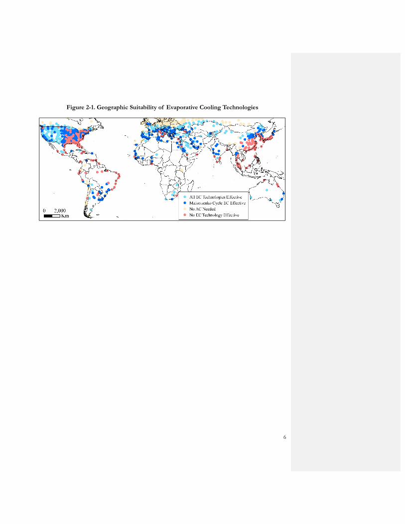
Temperature and humidity data for 1400 cities was obtained from American Society of Heating, Refrigeration and Air Conditioning Engineers, Inc. (ASHRAE 2009). ASHRAE guidelines were used to determine the most appropriate cooling technology for each city. A heat index of 26 °C., the upper bound of the ASHRAE summer comfort zone, was set as the minimum temperature for where RACs would be desired. A maximum dew-point temperature of 20 °C, a suggested upper boundary for residential humidity levels (Coolerado, 2012), was chosen. As direct ECs increase the humidity of the air, a wet-bulb temperature of 20 °C was chosen for their upper humidity limit. In locations where ECs were applicable, it was assumed that cooling was not needed during summer storms or monsoons.

The boundary conditions used in the suitability analysis are summarized in Table 2-1. As mentioned earlier, the direct and M-cycle ECs represent the two ends of the geographic spectrum of where ECs can be deployed. As a result, in cities where direct evaporative coolers are suitable, all other evaporative cooling technology is also suitable. In areas where M-cycle ECs are determined to be deployable, other technologies may also be suitable, however, only M-cycle ECs are guaranteed to be effective.

The results were entered into ArcGIS, a geographic information systems software, to be mapped. Because the dataset provided by ASHRAE did not contain geographic coordinates, the results were joined to an existing point shapefile1 that matched the city name with the geographic coordinates. One thousand and fifty cities matched successfully, which became the dataset used for all further analysis.

Table 2-1. Boundary Conditions used in EC Suitability Analysis

Technology Climatic Extent

No AC Technology Needed Heat index < 26 deg. C

M-Cycle EC Effective Dew Point Temp. < 20 deg. C

Direct and all other ECs Effective Wet-bulb Temp. < 20 deg. C

No EC Technology Effective All other Climate zones

2.2. Results and Discussion

Figure 3 illustrates the areas where evaporative cooling is effective. Direct ECs and all other evaporative cooling technologies are effective for 40% of the cities where RACs are likely to be deployed. The M-Cycle EC adds 200 cities to this count, increasing total EC coverage to 69%. Seventeen of the 50 most populated metropolitan areas of the world (Sivak 2009) are included in this count (labeled in blue in Figure 3-2). Replacing vapor compression RACs with ECs in these cities would have the largest impact on reducing global greenhouse gas emissions. In addition, in many of these cities, RACs contribute significantly to the total electricity load, leading to supply shortages during peak demand times (Lin & Rosenquist 2008; Sathaye & Gupta 2010). ECs, as the most energy efficient RAC, can help reduce these shortages.

1 A shapefile is a geospatial vector data format for geographic information systems software.

6

Figure 2-1. Geographic Suitability of Evaporative Cooling Technologies

7

3. Water Consumption of Evaporative Coolers

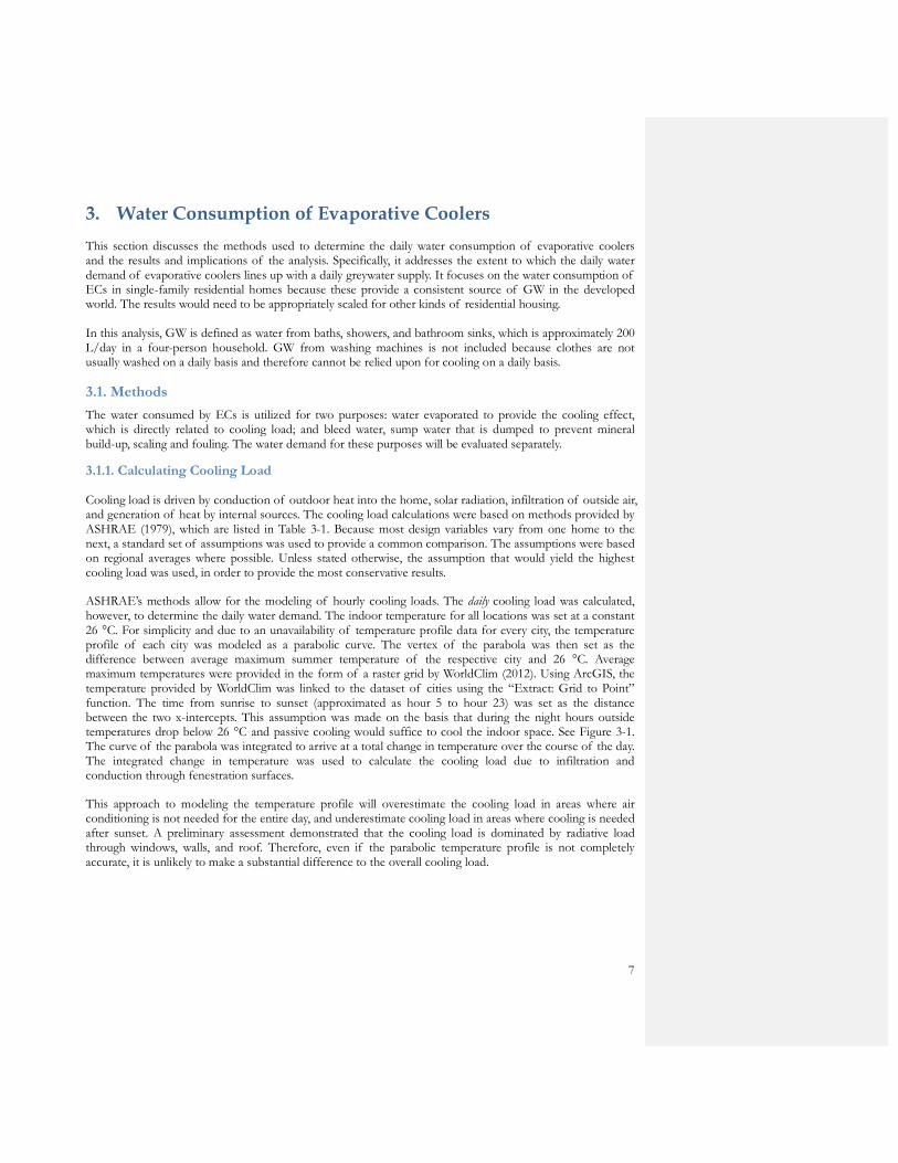
This section discusses the methods used to determine the daily water consumption of evaporative coolers and the results and implications of the analysis. Specifically, it addresses the extent to which the daily water demand of evaporative coolers lines up with a daily greywater supply. It focuses on the water consumption of ECs in single-family residential homes because these provide a consistent source of GW in the developed world. The results would need to be appropriately scaled for other kinds of residential housing. In this analysis, GW is defined as water from baths, showers, and bathroom sinks, which is approximately 200 L/day in a four-person household. GW from washing machines is not included because clothes are not usually washed on a daily basis and therefore cannot be relied upon for cooling on a daily basis.

3.1. Methods

The water consumed by ECs is utilized for two purposes: water evaporated to provide the cooling effect, which is directly related to cooling load; and bleed water, sump water that is dumped to prevent mineral build-up, scaling and fouling. The water demand for these purposes will be evaluated separately.

3.1.1. Calculating Cooling Load

Cooling load is driven by conduction of outdoor heat into the home, solar radiation, infiltration of outside air, and generation of heat by internal sources. The cooling load calculations were based on methods provided by ASHRAE (1979), which are listed in Table 3-1. Because most design variables vary from one home to the next, a standard set of assumptions was used to provide a common comparison. The assumptions were based on regional averages where possible. Unless stated otherwise, the assumption that would yield the highest cooling load was used, in order to provide the most conservative results.

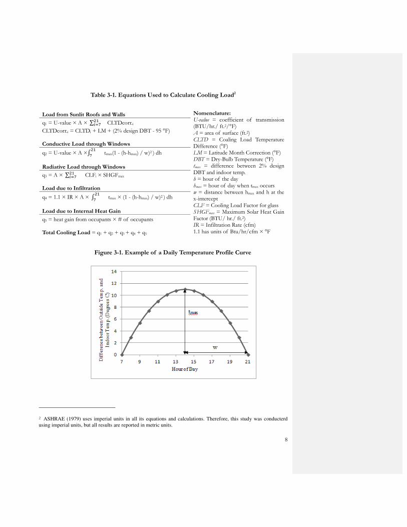
ASHRAE’s methods allow for the modeling of hourly cooling loads. The daily cooling load was calculated, however, to determine the daily water demand. The indoor temperature for all locations was set at a constant 26 °C. For simplicity and due to an unavailability of temperature profile data for every city, the temperature profile of each city was modeled as a parabolic curve. The vertex of the parabola was then set as the difference between average maximum summer temperature of the respective city and 26 °C. Average maximum temperatures were provided in the form of a raster grid by WorldClim (2012). Using ArcGIS, the temperature provided by WorldClim was linked to the dataset of cities using the “Extract: Grid to Point” function. The time from sunrise to sunset (approximated as hour 5 to hour 23) was set as the distance between the two x-intercepts. This assumption was made on the basis that during the night hours outside temperatures drop below 26 °C and passive cooling would suffice to cool the indoor space. See Figure 3-1. The curve of the parabola was integrated to arrive at a total change in temperature over the course of the day. The integrated change in temperature was used to calculate the cooling load due to infiltration and conduction through fenestration surfaces.

This approach to modeling the temperature profile will overestimate the cooling load in areas where air conditioning is not needed for the entire day, and underestimate cooling load in areas where cooling is needed after sunset. A preliminary assessment demonstrated that the cooling load is dominated by radiative load through windows, walls, and roof. Therefore, even if the parabolic temperature profile is not completely accurate, it is unlikely to make a substantial difference to the overall cooling load.

8

Table 3-1. Equations Used to Calculate Cooling Load2

Load from Sunlit Roofs and Walls Nomenclature: U-value = coefficient of transmission (BTU/hr./ ft.2/°F) A = area of surface (ft.2) CLTD = Coaling Load Temperature Difference (°F) LM = Latitude Month Correction (°F) DBT = Dry-Bulb Temperature (°F) tmax = difference between 2% design DBT and indoor temp. h = hour of the day hmax = hour of day when tmax occurs w = distance between hmax and h at the x-intercept CLF = Cooling Load Factor for glass SHGFmax = Maximum Solar Heat Gain Factor (BTU/ hr./ ft.2) IR = Infiltration Rate (cfm) 1.1 has units of Btu/hr/cfm × °F

q1 = U-value × A × ∑����� CLTDcorr.i

CLTDcorr.i = CLTDi + LM + (2% design DBT - 95 °F)

Conductive Load through Windows

q2 = U-value × A ×���

� tmax(1 - (h-hmax) / w)2 ) dh

Radiative Load through Windows

q3 = A × ∑����� CLFi × SHGFmax Load due to Infiltration

q4 = 1.1 × IR × A × ���

� tmax × (1 - (h-hmax) / w)2 ) dh

Load due to Internal Heat Gain

q5 = heat gain from occupants × # of occupants Total Cooling Load = q1 + q2 + q3 + q4 + q5

Figure 3-1. Example of a Daily Temperature Profile Curve

2 ASHRAE (1979) uses imperial units in all its equations and calculations. Therefore, this study was conducterd

using imperial units, but all results are reported in metric units.

9

Heat gain from solar radiation onto the walls, roof, and directly into the home through fenestration depends on geographical latitude, the time of the year and day, and the orientation of the surface. ASHRAE provides the hourly cooling load factors (CLFs) for various surfaces. For fenestration, the product of the summation of CLFs for unshaded glass and the solar maximum heat gain factor (SHGFmax) were taken, for the specific the latitude and the months of July and January for northern and southern latitudes, respectively. For opaque surfaces (roof and walls), ASHRAE provides the CLF for radiation and the cooling load due to conduction as one value – the cooling load temperature difference (CLTD). The hourly CLTDs were summed, assuming dark surfaces for the walls and roof of the home and correcting for the latitude and temperature difference for each location.

Although house sizes vary across the globe, they can be divided into two broad categories: average house size in the United States, Canada, and Australia (200 m2); and average house size of the rest of the world (100 m2) (BBC 2009). These categories were used to determine the dimensions of the cooled space in the model. For simplicity, the modeled home was made up of a single story, a square floor plan, a flat roof, 2.5 m walls, and fenestration area of one fourth of the wall’s surface area.

Coefficients of transmission (U-values), which represent the amount of heat that can be conducted through a given material, and rate of infiltration can vary significantly from one home to the next. However, the U-values that reflected minimal insulation and maximum heat transfer into the cooled space were chosen: 0.76 W/m2K for the roof, 0.51 W/m2K for the walls, and 5.68 W/m2K for windows. A standard infiltration rate (IR) for residential homes of 0.033 L/s was assumed (ASHRAE 1979).

Sources of internal heat generation include occupant metabolism, lighting, and appliances. It was assumed that lighting and load due to appliances would be negligible in residential homes compared to the overall heat gain over the course of a summer day. Four occupants who are seated and/or doing light work were assumed to calculate internal heat generation.

3.1.2. Water Consumption Due to Cooling

The amount of water consumed by an EC for a given cooling load varies widely from one model to the next, based on the components used. Water efficiency varies from 0.45 megajoules cooling delivered per liter of water consumed (MJ/L) to 2 MJ/L. Older and cheaper models tend to use more water than newer more expensive ones. In addition, an EC’s water efficiency will decrease if the actual cooling demand strays too far from the EC’s rated capacity. The M-cycle EC reports an average rate of 1.44 MJ/L, but at peak temperatures it produces 1.33 MJ/L (Kozubal and Slayzak 2010). In this study 1.33 MJ/L was used. The daily cooling load was divided by this value to determine water consumption due to cooling.

3.1.3. Sensitivity Analysis

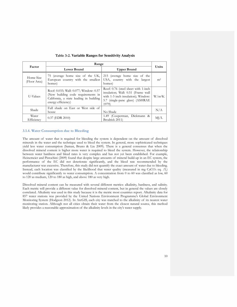
Many of the factors that make up the water consumption calculation can be highly variable and change the final outcome significantly. To address this issue, a sensitivity analysis was conducted on a number of variables. The analysis compares the location-based water consumption range established by the model, to the amount that each variable can increase that range. The variable and their ranges are listed in Table 3-2.

10

Table 3-2. Variable Ranges for Sensitivity Analysis

Factor Range

Units Lower Bound Upper Bound

Home Size (Floor Area)

75 (average home size of the UK, European country with the smallest homes)

215 (average home size of the USA, country with the largest homes)

m2

U-Values

Roof: 0.033; Wall: 0.077; Window: 0.57 (New building code requirements in California, a state leading in building energy efficiency)

Roof: 0.76 (steel sheet with 1-inch insulation; Wall: 0.51 (Frame wall with 1-3 inch insulation); Window: 5.7 (single-pane glass) (ASHRAE 1979)

W/m2K

Shade Full shade on East or West side of house No Shade

N/A

Water Efficiency

0.37 (EDR 2010) 1.49 (Cooperman, Diekmann & Brodrick 2011)

MJ/L

3.1.4. Water Consumption due to Bleeding The amount of water that is required for bleeding the system is dependent on the amount of dissolved minerals in the water and the technique used to bleed the system. In general, more sophisticated techniques yield less water consumption (Saman, Bruno & Liu 2009). There is a general consensus that when the dissolved mineral content is higher more water is required to bleed the system. However, the relationship between water hardness and bleed rates is very complex and has not yet been established. For example, Heinemeier and Pistochini (2009) found that despite large amounts of mineral build-up in an EC system, the performance of the EC did not deteriorate significantly, and the bleed rate recommended by the manufacturer was excessive. Therefore, this study did not quantify the exact amount of water due to bleeding. Instead, each location was classified by the likelihood that water quality (measured in mg CaCO3 eq. /L) would contribute significantly to water consumption. A concentration from 0 to 60 was classified as low, 60 to 120 as medium, 120 to 180 as high, and above 180 as very high. Dissolved mineral content can be measured with several different metrics: alkalinity, hardness, and salinity. Each metric will provide a different value for dissolved mineral content, but in general the values are closely correlated. Alkalinity was used in this study because it is the metric most countries report. Alkalinity data for 857 water stations was provided by the United Nations Environment Programme’s Global Environment Monitoring System (Hodgson 2012). In ArcGIS, each city was matched to the alkalinity of its nearest water monitoring station. Although not all cities obtain their water from the closest natural source, this method likely provides a reasonable approximation of the alkalinity levels in the city’s water supply.

11

3.2. Results and Discussion

3.2.1. Water Consumption of Evaporative Coolers

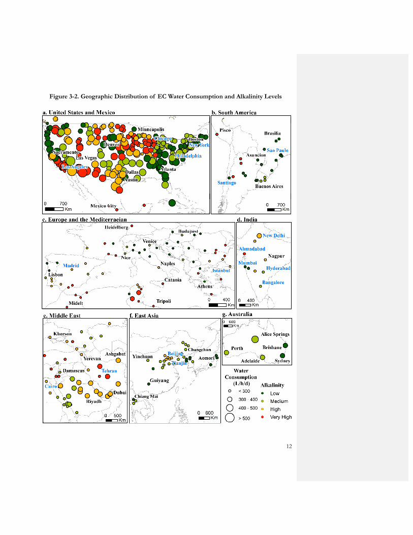
Figure 3-2 illustrates the daily, per household water consumption of ECs. This is the amount of water that is required if the EC is running at all times of the day when temperatures are above 26 °C. Therefore, it is an overestimate of water consumption during weekdays, when much of the day is spent at work, or for low-income populations, where the amount of cooling that the EC provides is limited for financial reasons. In most cities of Europe, East Asia, and South America water consumption due to cooling is less than 300 liters/household/day (L/hd/d). At this rate, GW produced by a four-person household can supply most of the water demanded by an EC. In most cities in the Middle East, South Asia, Australia and the United States ECs consume between 300 and 500 L/hd/d. GW can supply 40 to 67% of this demand, however, this percentage will increase with more people per household. Since water scarcity is a problem in these regions of the world (Smakhtin et al., 2004), utilizing GW in evaporative cooling will likely remove a significant barrier to the deployment of ECs and should be seriously considered.

Figure 3-2 also illustrates the impact that alkalinity is likely to have on EC water consumption. The Mediterranean, the Middle East, Northern India, and the Midwestern and Southwestern United States are regions with high alkalinity levels. There is a high likelihood that bleeding of ECs in these regions will contribute significantly to its water consumption. Future research is needed be able to quantify this contribution. In these regions especially, care should be taken to encourage the use of ECs with sophisticated bleeding techniques, such as timed drain-off or salinity-level monitoring systems.

Of the 17 cities recognized to have the largest populations, and therefore, the largest potential for global impact, deployment efforts should first be focused on areas where water scarcity is not a problem, such as Philadelphia, Chicago, Sao Paulo. On the other hand, Mumbai, São Paulo, and Santiago all have low alkalinity levels and water consumption due to bleeding is likely to be minimal.

12

Figure 3-2. Geographic Distribution of EC Water Consumption and Alkalinity Levels

13

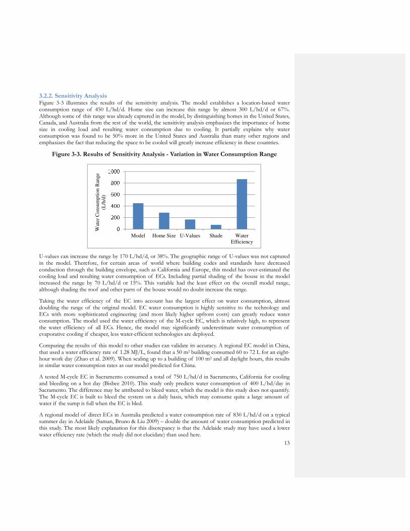
3.2.2. Sensitivity Analysis Figure 3-3 illustrates the results of the sensitivity analysis. The model establishes a location-based water consumption range of 450 L/hd/d. Home size can increase this range by almost 300 L/hd/d or 67%. Although some of this range was already captured in the model, by distinguishing homes in the United States, Canada, and Australia from the rest of the world, the sensitivity analysis emphasizes the importance of home size in cooling load and resulting water consumption due to cooling. It partially explains why water consumption was found to be 50% more in the United States and Australia than many other regions and emphasizes the fact that reducing the space to be cooled will greatly increase efficiency in these countries.

Figure 3-3. Results of Sensitivity Analysis - Variation in Water Consumption Range

U-values can increase the range by 170 L/hd/d, or 38%. The geographic range of U-values was not captured in the model. Therefore, for certain areas of world where building codes and standards have decreased conduction through the building envelope, such as California and Europe, this model has over-estimated the cooling load and resulting water consumption of ECs. Including partial shading of the house in the model increased the range by 70 L/hd/d or 15%. This variable had the least effect on the overall model range, although shading the roof and other parts of the house would no doubt increase the range.

Taking the water efficiency of the EC into account has the largest effect on water consumption, almost doubling the range of the original model. EC water consumption is highly sensitive to the technology and ECs with more sophisticated engineering (and most likely higher upfront costs) can greatly reduce water consumption. The model used the water efficiency of the M-cycle EC, which is relatively high, to represent the water efficiency of all ECs. Hence, the model may significantly underestimate water consumption of evaporative cooling if cheaper, less water-efficient technologies are deployed.

Comparing the results of this model to other studies can validate its accuracy. A regional EC model in China, that used a water efficiency rate of 1.28 MJ/L, found that a 50 m2 building consumed 60 to 72 L for an eight- hour work day (Zhao et al. 2009). When scaling up to a building of 100 m2 and all daylight hours, this results in similar water consumption rates as our model predicted for China.

A tested M-cycle EC in Sacramento consumed a total of 750 L/hd/d in Sacramento, California for cooling and bleeding on a hot day (Bisbee 2010). This study only predicts water consumption of 400 L/hd/day in Sacramento. The difference may be attributed to bleed water, which the model is this study does not quantify. The M-cycle EC is built to bleed the system on a daily basis, which may consume quite a large amount of water if the sump is full when the EC is bled.

A regional model of direct ECs in Australia predicted a water consumption rate of 830 L/hd/d on a typical summer day in Adelaide (Saman, Bruno & Liu 2009) – double the amount of water consumption predicted in this study. The most likely explanation for this discrepancy is that the Adelaide study may have used a lower water efficiency rate (which the study did not elucidate) than used here.

02004006008001000Model Home Size U-Values Shade Water

Efficiency

Wat

er

Co

nsu

mp

tio

n R

ange

(L/h

/d)

14

4. Greywater for Evaporative Cooling

4.1. Technical Feasibility.

The model demonstrates that GW can supply 40 to 100% of the water consumed by ECs. To do so, however, a GW system needs to treat the water so that it can safely be evaporated into the indoor space. Similar to a GW system for toilet flushing, it will need a sedimentation tank or filter to remove suspended particles; a biological control unit to control for fouling and odor, and some type of disinfection.

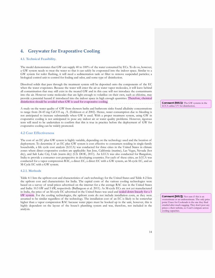
Dissolved solids that pass through the treatment system will be deposited onto the components of the EC when the water evaporates. Because the water will enter the air as water vapor molecules, it will leave behind all contamination that may still exist in the treated GW and in this case will not introduce the contaminants into the air. However some molecules that are light enough to volatilize on their own, such as chlorine, may provide a potential hazard if introduced into the indoor space in high enough quantities. Therefore, chemical disinfection should be avoided when GW is used for evaporative cooling.

A study on the water quality of GW from showers baths and bathroom sinks found alkalinity concentrations to range from 24-43 mg CaCO3 eq. /L (Erikkson et al 2002). Hence, water consumption due to bleeding is not anticipated to increase substantially when GW is used. With a proper treatment system, using GW in evaporative cooling is not anticipated to pose any indoor air or water quality problems. However, rigorous tests will need to be undertaken to confirm that this is true in practice before the deployment of GW for evaporative cooling can be widely promoted.

4.2 Cost Effectiveness

The cost of an EC plus GW system is highly variable, depending on the technology used and the location of deployment. To determine if an EC plus GW system is cost effective to consumers residing in single-family households, a life cycle cost analysis (LCCA) was conducted for three cities in the United States in climate zones where direct evaporative coolers are applicable: San Jose, California (marine), Las Vegas, Nevada (hot dry), and Salt Lake City, Utah (warm dry) (U.S. DOE, 2011). An LCCA was also conducted for Bangalore, India to provide a consumer cost perspective in developing countries. For each of these cities, an LCCA was conducted for a vapor compression RAC, a direct EC, a direct EC with a GW system, an M-cycle EC, and an M-Cycle EC with a GW system.

4.2.1. Methods

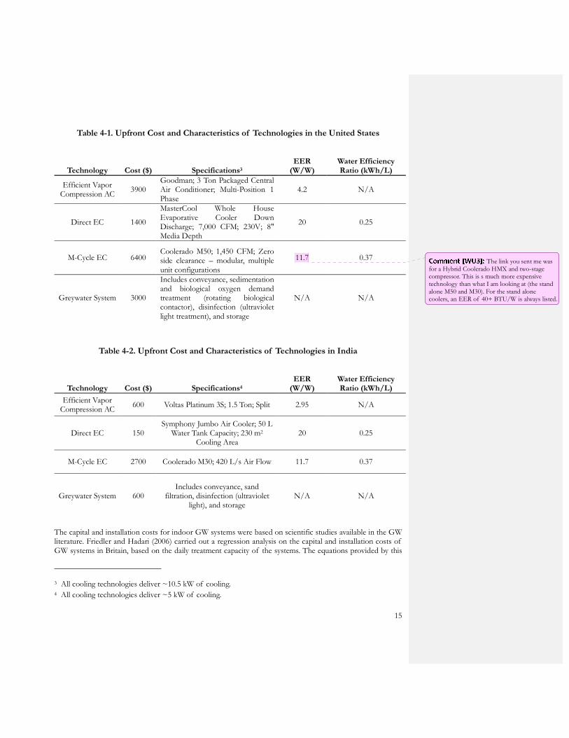
Table 4-1 lists the upfront cost and characteristics of each technology for the United States and Table 4-2 lists the upfront cost and characteristics for India. The capital costs of the various cooling technologies were based on a survey of retail prices advertised on the internet for a the average RAC size in the United States and India: 10.5 kW and 5 kW, respectively (Baillargeon et al. 2011). As M-cycle ECs are not yet manufactured in India, the price of an M-cycle EC advertised in the United States was used and scaled down linearly for a 5 kW system. For the cooling technologies, the upfront costs do not include installation costs, as they were assumed to be similar regardless of the technology. The installation cost of an EC is likely to be somewhat higher than a vapor compression RAC because water pipes must be hooked up to the unit, however, this is highly dependent on the layout of the house’s plumbing system and was, therefore, not included in the analysis.

Comment [WU1]: The GW systems in the LCCA utilize UV for disinfection.

Comment [WU2]: Not sure if this is an overestimate or an underestimate. The only price point I have for Coolerado is the one they final emailed after much nagging. They don’t post any prices o their website, so I can’t compare across cooling capacities.

15

Table 4-1. Upfront Cost and Characteristics of Technologies in the United States

Technology Cost ($) Specifications3 EER

(W/W) Water Efficiency Ratio (kWh/L)

Efficient Vapor Compression AC

3900 Goodman; 3 Ton Packaged Central Air Conditioner; Multi-Position 1 Phase

4.2 N/A

Direct EC 1400

MasterCool Whole House Evaporative Cooler Down Discharge; 7,000 CFM; 230V; 8" Media Depth

20 0.25

M-Cycle EC 6400 Coolerado M50; 1,450 CFM; Zero side clearance – modular, multiple unit configurations

11.7 0.37

Greywater System 3000

Includes conveyance, sedimentation and biological oxygen demand treatment (rotating biological contactor), disinfection (ultraviolet light treatment), and storage

N/A N/A

Table 4-2. Upfront Cost and Characteristics of Technologies in India

Technology Cost ($) Specifications4 EER

(W/W) Water Efficiency Ratio (kWh/L)

Efficient Vapor Compression AC

600 Voltas Platinum 3S; 1.5 Ton; Split 2.95 N/A

Direct EC 150 Symphony Jumbo Air Cooler; 50 L

Water Tank Capacity; 230 m2 Cooling Area

20 0.25

M-Cycle EC 2700 Coolerado M30; 420 L/s Air Flow 11.7 0.37

Greywater System 600 Includes conveyance, sand

filtration, disinfection (ultraviolet light), and storage

N/A N/A

The capital and installation costs for indoor GW systems were based on scientific studies available in the GW literature. Friedler and Hadari (2006) carried out a regression analysis on the capital and installation costs of GW systems in Britain, based on the daily treatment capacity of the systems. The equations provided by this

3 All cooling technologies deliver ~10.5 kW of cooling. 4 All cooling technologies deliver ~5 kW of cooling.

Comment [WU3]: The link you sent me was for a Hybrid Coolerado HMX and two-stage compressor. This is s much more expensive technology than what I am looking at (the stand alone M50 and M30). For the stand alone coolers, an EER of 40+ BTU/W is always listed.

16

study were used to determine the upfront cost of GW system in the United States for a capacity of 200 L/day. Godfrey et al. (2009) carried out an itemized cost analysis on the capital and installation costs of an indoor GW system built in India. The costs provided by this study were linearly scaled down to determine the cost of a 200 L/day-system in Bangalore.

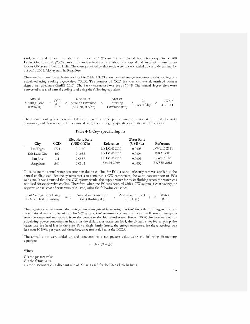
The specific inputs for each city are listed in Table 4-3. The total annual energy consumption for cooling was calculated using cooling degree days (CCD). The number of CCD for each city was determined using a degree day calculator (BizEE 2012). The base temperature was set at 79 °F. The annual degree days were converted to a total annual cooling load using the following equation:

Annual Cooling Load

(kWh/yr) =

CCD (°F)

× U-value of

Building Envelope (BTU/h/ft.2/°F)

× Area of Building

Envelope (ft.2) ×

24 hours/day

× 1 kWh /

3412 BTU

The annual cooling load was divided by the coefficient of performance to arrive at the total electricity consumed, and then converted to an annual energy cost using the specific electricity rate of each city.

Table 4-3. City-Specific Inputs

City CCD Electricity Rate

(USD/kWh) Reference Water Rate (USD/L) Reference

Las Vegas 1721 0.1160 US DOE 2011 0.0005 LVVWD 2011

Salt Lake City 409 0.1035 US DOE 2011 0.0004 WRA 2005

San Jose 111 0.0987 US DOE 2011 0.0009 SJWC 2012

Bangalore 543 0.0804 Swathi 2009 0.0002 BWSSB 2012

To calculate the annual water consumption due to cooling for ECs, a water efficiency rate was applied to the annual cooling load. For the systems that also contained a GW component, the water consumption of ECs was zero. It was assumed that the GW system would also supply water for toilet flushing when the water was not used for evaporative cooling. Therefore, when the EC was coupled with a GW system, a cost savings, or negative annual cost of water was calculated, using the following equation:

Cost Savings from Using GW for Toilet Flushing

= ( Annual water used for

toilet flushing (L) -

Annual water used for EC (L)

) × Water Rate

The negative cost represents the savings that were gained from using the GW for toilet flushing, as this was an additional monetary benefit of the GW system. GW treatment systems also use a small amount energy to treat the water and transport it from the source to the EC. Friedler and Hadari (2006) derive equations for calculating power consumption based on the daily water treatment load, the elevation needed to pump the water, and the head loss in the pipe. For a single-family home, the energy consumed for these services was less than 50 kWh per year, and therefore, were not included in the LCCA.

The annual costs were added up and converted to a net present value using the following discounting equation:

P = F / [(1 + i)n]

Where

P is the present value F is the future value i is the discount rate - a discount rate of 2% was used for the US and 6% in India

17

n is the number of year - a life-span of 20 years was used for both countries

4.2.2. Discussion and Results

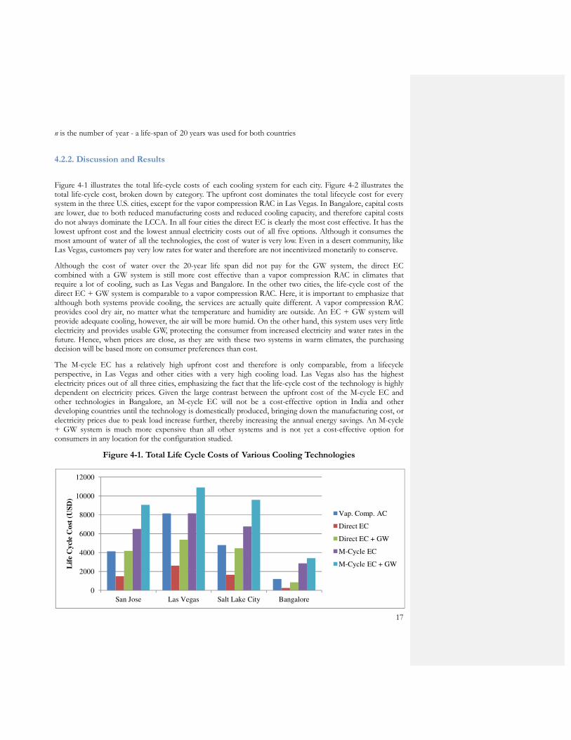
Figure 4-1 illustrates the total life-cycle costs of each cooling system for each city. Figure 4-2 illustrates the total life-cycle cost, broken down by category. The upfront cost dominates the total lifecycle cost for every system in the three U.S. cities, except for the vapor compression RAC in Las Vegas. In Bangalore, capital costs are lower, due to both reduced manufacturing costs and reduced cooling capacity, and therefore capital costs do not always dominate the LCCA. In all four cities the direct EC is clearly the most cost effective. It has the lowest upfront cost and the lowest annual electricity costs out of all five options. Although it consumes the most amount of water of all the technologies, the cost of water is very low. Even in a desert community, like Las Vegas, customers pay very low rates for water and therefore are not incentivized monetarily to conserve.

Although the cost of water over the 20-year life span did not pay for the GW system, the direct EC combined with a GW system is still more cost effective than a vapor compression RAC in climates that require a lot of cooling, such as Las Vegas and Bangalore. In the other two cities, the life-cycle cost of the direct EC + GW system is comparable to a vapor compression RAC. Here, it is important to emphasize that although both systems provide cooling, the services are actually quite different. A vapor compression RAC provides cool dry air, no matter what the temperature and humidity are outside. An EC + GW system will provide adequate cooling, however, the air will be more humid. On the other hand, this system uses very little electricity and provides usable GW, protecting the consumer from increased electricity and water rates in the future. Hence, when prices are close, as they are with these two systems in warm climates, the purchasing decision will be based more on consumer preferences than cost.

The M-cycle EC has a relatively high upfront cost and therefore is only comparable, from a lifecycle perspective, in Las Vegas and other cities with a very high cooling load. Las Vegas also has the highest electricity prices out of all three cities, emphasizing the fact that the life-cycle cost of the technology is highly dependent on electricity prices. Given the large contrast between the upfront cost of the M-cycle EC and other technologies in Bangalore, an M-cycle EC will not be a cost-effective option in India and other developing countries until the technology is domestically produced, bringing down the manufacturing cost, or electricity prices due to peak load increase further, thereby increasing the annual energy savings. An M-cycle + GW system is much more expensive than all other systems and is not yet a cost-effective option for consumers in any location for the configuration studied.

Figure 4-1. Total Life Cycle Costs of Various Cooling Technologies

0

2000

4000

6000

8000

10000

12000

San Jose Las Vegas Salt Lake City Bangalore

Lif

e C

ycle

Co

st (

US

D)

Vap. Comp. AC

Direct EC

Direct EC + GW

M-Cycle EC

M-Cycle EC + GW

18

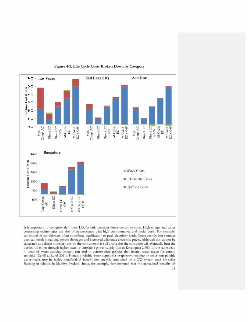
Figure 4-2. Life Cycle Costs Broken Down by Category

It is important to recognize that these LCCAs only consider direct consumer costs. High energy and water consuming technologies are also often associated with high environmental and social costs. For example, residential air conditioners often contribute significantly to peak electricity loads. Consequently, hot summer days can result in national power shortages and increased wholesale electricity prices. Although this cannot be calculated as a direct monetary cost to the consumer, it is still a cost that the consumer will eventually bear the burden of, either through higher taxes or unreliable power supply (Lin & Rosenquist 2008). In the same vein, in areas of water scarcity, drought can lead to conservation policies that restrict water usage for certain activities (Cahill & Lund 2011). Hence, a reliable water supply for evaporative cooling or other non-potable water needs may be highly beneficial. A benefit-cost analysis conducted on a GW system used for toilet flushing in schools in Madhya Pradesh, India, for example, demonstrated that the annualized benefits of

-6001400340054007400940011400V

ap.

Co

mp

. A

C

Dir

ect

EC

Dir

ect

EC

+ G

W

M-C

ycle

EC

M-C

ycl

e

EC

+ G

W

Lif

etim

e C

ost

(U

SD

)

Las Vegas

Vap.

Co

mp

. A

C

Dir

ect

EC

Dir

ect

EC

+ G

W

M-C

ycle

EC

M-C

ycl

e

EC

+ G

W

Salt Lake City

Vap.

Co

mp

. A

C

Dir

ect

EC

Dir

ect

EC

+ G

W

M-C

ycle

EC

M-C

ycl

e

EC

+ G

W

San Jose

-600

400

1400

2400

3400

4400

Vap. C

om

p.

AC

Dir

ect

EC

Dir

ect

EC

+

GW

M-C

ycle

EC

M-C

ycle

EC

+ G

W

Lif

etim

e C

ost

(U

SD

)

Bangalore

Water Costs

Electricity Costs

Upfront Costs

19

avoiding building new infrastructure and increasing water availability amounted to $1800. The annualized system costs only added up to $260 – a cost benefit ratio of 6.9 (Godfrey et al. 2009). Hence, by only capturing the consumer costs, the LCCA does not include the full costs or benefits of each system to society.

As mentioned in the introduction, garden irrigation is also a common use for GW. Because GW systems for garden irrigation are a lot less complex, their upfront costs are also significantly lower. A brief cost survey yielded the equipment and installation costs to range from $200 to $1000 in the United States, depending on the complexity of the system. Therefore, households that consume a lot of water for irrigation may find that using GW for this purpose is more cost-effective than using GW for evaporative cooling. Moreover, if the GW is used to irrigate trees that shade the house, the GW would indirectly be used for cooling as well.

20

5. Summary and Conclusions

ECs provide significant gains in energy efficiency compared to vapor compression RACs, but simultaneously greatly increase the RAC’s onsite water demand. This can be a major deployment barrier in areas of the world that suffer from water scarcity. To address this concern, the study determined where in the world evaporative cooling is suitable, conservatively estimated the water consumption of ECs in these cities, and explored the potential of greywater in reducing the consumption of potable water in ECs. ECs covered 69% of the cities where RACs are likely to be deployed, including 17 of the world’s 50 most populous cities. Water consumption due to ECs ranged from 200 to 650 L/hd/d, with the potential for GW to provide 100% to 40% of this amount, respectively. In the Mediterranean, the Middle East, Northern India, and the Midwestern and Southwestern United States alkalinity levels are high and water used for bleeding will likely contribute substantially to EC water consumption. Although technically feasible, upfront costs for household GW systems are currently high. In both developed and developing parts of the world, however, a direct EC and GW system is cost competitive with conventional vapor compression air conditioners. Due to the high capital cost of M-cycle ECs, an M-cycle EC and GW system is not currently cost competitive. Both the LCCA and case studies demonstrate that in regions of the world that face problems of water scarcity, the benefits of a GW system for ECs appreciably outweigh the costs. At the moment, the use of greywater in evaporative cooling is a new concept and future research is needed to test its applicability and practicality.

21

Acknowledgments

Thanks are owed to Kelly Hodgson at the UNEP GEMS Water Progamme. A large portion of this analysis would not have been possible without the water quality data that she consolidated and organized specifically for this study. Duncan Callaway, assistant professor at the Energy and Resources Group, provided very helpful feedback and suggestions, and we thank him for his contribution.

22

References

[ASHRAE] American Society of Heating, Refrigeration and Air Conditioning Engineers, Inc. 1979. Cooling and Heating Load Manual. New York. [ASHRAE] American Society of Heating, Refrigeration and Air Conditioning Engineers, Inc. 2009. Fundamentals. New York. [BBC] BBC News Magazine. 2009. “Room to swing a cat? Hardly”. August 15, 2009. Bisbee, D. 2010. Technology Evaluation Report: The CooleradoTM. Sacramento, Calif.: Customer Advanced Technologies Program, Sacramento Municipal Utilities District. BizEE. 2012. Degree Days: Weather Data for Energy Professionals. http://www.degreedays.net. Baillargeon, P., N. Michaud, L. Tossou, P. Waide. Cooling Benchmarking Study, Part 1: Mapping Component Report. The Collaborative Labeling and Appliance Program. Washington, DC. June 2011. Bom, G.J., R. Foster, E. Dijkstra, M. Tummers. 1999. Evaporative Air-Conditioning: Applications for Environmentally Friendly Cooling. World Bank Technical Paper No. 421. Cahil, R., and J. Lund. 2011. Residential Water Conservation in Australia and California. Department of Civil and Environmental Engineering, University of California, Davis Coolerado Corporation. 2012. Coolerado Heat and Mass Exchanger (HMX) World Performance Table – SI Units. Denver, Colorado. http://www.coolerado.com/pdfs/CooleradoHMXPerformanceSI.pdf. Cooperman, A., J. Dieckmann, & J. Brodrick. “Water/Electricity Tradeoffs”. Emerging Technologies, ASHRAE Journal (December): 118-119. Ecodesign. 2008. Preparatory study on the environmental performance of residential room conditioning appliances (airco and ventilation), Draft Report of Task 2. http://www.ebpg.bam.de/de/ebpg_medien/tren10/010_studyf_08-07_airco_part2.pdf. [EDR] Energy Design Resources. 2010. “Evaporative Cooling: Saving More Ways in Energy than Ever”. Energy Design Resources, e-News (71): 1-4. Eriksson, E., K. Auffarth, M. Henze & A. Ledin. 2002. “Characteristics of grey wastewater”. Urban Water, 4: 85–104. Friedler, E & M. Hadari. 2006. “Economic feasibility of on-site greywater reuse in multi-storey buildings”. Desalination 190: 221–234. Godfrey, S, P. Labhasetwarb, & S. Wate. 2009. “Greywater reuse in residential schools in Madhya Pradesh, India—A case study of cost–benefit analysis”. Resources, Conservation and Recycling 53: 287–293. Heidarinejad, G., M. Bozorgmehr, S. Delfani, & J. Esmaeelian. 2009. “Experimental investigation of two-stage indirect/direct evaporative cooling system in various climatic conditions”. Building and Environment 44: 2073–2079. Heinemeier, K.H. & T. E. Pistochini. 2009. Water Management for Indirect-Direct Evaporative Air Conditioning, Final

23

Report. Davis, Calif: Western Cooling Efficiency Center. Hodgson, Kelly (United Nations Environment Programme). 2012. Personal Communication. February 20. Hsieh, C.M., T. Aramaki & K. Hanaki. 2007. “The feedback of heat rejection to air conditioning load during the nighttime in subtropical climate”. Energy and Buildings, 39: 1175–1182. Kozubal, E. & S. Slayzak. 2010. Coolerado 5 Ton RTU Performance: Western Cooling Challenge Results. NREL/TP-5500-46524. Golden, Colo: National Renewable Energy Laboratory. Lin, J., & G. Rosenquist. 2008. “Stay cool with less work: China’s new energy-efficiency standards for air conditioners”. Energy Policy 36: 1090–1095. [LVVWD] Las Vegas Valley Water District. 2011. Rates and Usage Thresholds. http://www.lvvwd.com/custserv/billing_rates_thresholds.html. March, J. G., M. Gual, F. Orozco. 2004. “Experiences on greywater re-use for toilet flushing in a hotel (Mallorca Island, Spain)”. Desalination 164: 241-247. McNeil, M. A., & V. E. Letschert. 2008. Future Air Conditioning Energy Consumption in Developing Countries and what can be done about it: The Potential of Efficiency in the Residential Sector. Berkeley, Calif: Lawrence Berkeley National Laboratory. Nolde, E. 1999. “Greywater reuse systems for toilet flushing in multi-storey buildings - over ten years experience in Berlin”. Urban Water 1: 275-284. Nolde, E. 2005. “Greywater recycling systems in Germany - results, experiences and guidelines”Water Science & Technology 51(10): 203–210. Oasis Design. 2012. http://oasisdesign.net/. Paris S., C. Schlapp. 2010. “Greywater recycling in Vietnam — Application of the HUBER MBR process”. Desalination 250: 1027–103. Pistochini, T. & M. Modera. 2011. “Water-use efficiency for alternative cooling technologies in arid climates”. Energy and Buildings 43: 631–638. Rizwan, A.M., L.Y.C. Dennis & C. Liu. 2008. “A review on the generation, determination and mitigation of Urban Heat Island”. Journal of Environmental Sciences, 20: 120–128. [SJWC] San Jose Water Company. 2012. General Metered Service. http://www.sjwater.com/files/documents/schedule1_20120101.pdf Saman, W., F. Bruno, & M. Liu. 2009. Technical Background Research On Evaporative Air Conditioners And Feasibility Of Rating Their Water Consumption. Adelaide, Australia: University of South Australia. Sathaye J. & A. P. Gupta. 2010. Eliminating Electricity Deficit through Energy Efficiency in India: An Evaluation of Aggregate Economic and Carbon Benefit. Berkeley, Calif: Lawrence Berkeley National Laboratory. Smakhtin V., C. Revenga & P. Döll. 2004. “A Pilot Global Assessment of Environmental Water Requirements and Scarcity”. Water International 29(3): 307-317.

24

Swathi. 2009. “Bangalore Electricity Tariff Hike”. My Bangulru. Posted Nov. 26, 2009. http://www.mybengaluru.com/resources/2248-Bangalore-Electricity-Tariff-Hike.aspx [US DOE] Climate Specific Publications. Building America – Resources for Energy Efficient Homes. United States Department of Energy. May 3, 2011.

[US DOE] U.S. Electric Utility Companies and Rates: Look-up by Zipcode. United States Department of Energy. Feb. 2011. http://en.openei.org/datasets/node/899

Wen, Y. & Z. Lian. 2009. “Influence of air conditioners utilization on urban thermal Environment”. Applied Thermal Engineering, 29: 670–675. [WRA] Western Resource Advocates. 2005. Water Rate Structures in Utah: How Utah Cities Compare Using This Important Water Use Efficiency Tool. Boulder, Colo. Willis, R. M., R. A. Stewart, D. P. Giurco, M. R. Talebpour, & A. Mousavinejad. 2011. “End use water consumption in households: impact of socio-demographic factors and efficient devices”. Journal of Cleaner Production xxx: 1-9. WorldClim. 2010. “Current Conditions – 30 Arc-seconds (1 km)”. Global Climate Data. Berkeley, Calif: Museum of Vertebrate Zoology. Zhao, X., S. Yang, Z. Duan, & S. B. Riffat. 2009. “Feasibility study of a novel dew point air conditioning system for China building application”. Building and Environment 44: 1990–1999. U.S. Electric Utility Companies and Rates: Look-up by Zipcode. United States Department of Energy. Feb. 2011. http://en.openei.org/datasets/node/899

Las Vegas Valley Water District Tier 2 Rates - http://www.lvvwd.com/custserv/billing_rates_thresholds.html

Salt Lake City Public Utilities Tier 2 Rates -http://www.westernresourceadvocates.org/media/pdf/Utah%20Water%20Rate%20Analysis%20-%20300dpi.pdf

San Jose Water Company Tier 1 Rates - http://www.sjwater.com/files/documents/schedule1_20120101.pdf