adaptation of continuous descent and climb operational ... · (easyjet-retired) and guglielmo...
TRANSCRIPT

FACULTY OF ENGINEERING
Academic year 2012-2013
Master’s thesis submitted under the supervision of Prof. Ir. Jean-Jacques Speyer, the co-supervision of Prof. Dr. Ir. Patrick Hendrick, in order to be awarded the Master’s Degree of Applied Sciences
and Engineering: Electro-Mechanical
Engineering: Aeronautics
Adaptation of continuous descent and climb operational techniques at Brussels Airport
aiming at cost efficiency.
Author: Sam Peeters

2

3
Preface First, I would like to thank Prof. Ir. Jean-Jacques Speyer (Airbus-retired) and Prof. Dr. Ir. Patrick
Hendrick for providing this interesting Master thesis subject because air traffic management and all
related subjects fascinate me. The continuous follow-up and extensive communication with Prof.
Speyer was a great help to bring this Master thesis to a good end. I have also had a lot of help from
people of the aviation industry. Many thanks go to Liesbeth Peeters, Paul Hopff and Carlo
Vandersmissen of Belgocontrol for the good information, data and cooperation on several occasions.
Thanks to the efforts of Carl-Philippe Combes and Tom Vaes of Thomas Cook Airlines, Rudolf
Christen, CEO Aviaso and André Berger, Brecht Lievrouw and Laurens Wielfaert of Jetairfly, I could
check my calculations against real flight data so again thank you for that. I have also very much
appreciated the remarks and comments of Elmar Recker of the RMA and Capt. Peter Griffiths
(EasyJet-retired) and Guglielmo Guastalla of Eurocontrol who have contributed to this work in a very
positive way.
Last but not least, I thank my family for supporting me during this whole period and especially my
girlfriend Kathleen for her patience and good care.

4
Legal notice This documentation, material or product has been created by using the V-PAT tool, makes reference
to the V-PAT tool or contains software parts of the V-PAT tool. The V-PAT tool has been created and
made available by the European Organisation for the Safety of Air Navigation (EUROCONTROL).
EUROCONTROL is the exclusive owner of the V-PAT tool. All Rights reserved.

5
Summaries
English summary This Master thesis: “Adaptation of continuous descent and climb operational techniques at Brussels Airport aiming at cost efficiency” was written by Sam Peeters in the academic year 2012-2013 in order to be awarded the Master’s Degree of Applied Sciences and Engineering: Electro-Mechanical Engineering: Aeronautics.
Keywords:
Continuous descent operations, continuous climb operations, cost index, dynamic trajectory
allocation, energy management
Abstract:
Continuous descent and climb operations aim at reducing the fuel burn and emissions during
respectively the descent and climb phases. In this Master thesis, the optimal descent and climb
profiles, based on the aircraft performance and the restrictions in the Belgian airspace, are calculated
using the BADA database of Eurocontrol.
The optimal descent profiles are calculated by determining the ideal descent angle at every moment
during the descent. The optimal climb profiles are retrieved using the specific excess power and fuel
specific energy. The optimal profile depends on the cost index which reflects the ratio of cost of time
and cost of fuel. In this work, the profiles for minimum fuel burn (cost index equal to zero) and for
minimum time (cost index maximum) are calculated. The calculated profiles are then compared to
profiles retrieved from real flight data. For the climb profiles, this reveals that for the real flights
around 306 to 390kg of extra fuel is used, 2.7 to 3.4 minutes of extra time are needed and 3.4 to
17.2NM of extra track distances until the top of climb are flown, compared to the calculated climb
profiles. The parameters of the real descent profiles are corresponding quite well to the calculated
ones.
To account for a multiple aircraft situation for continuous descents, a simulation is performed. This is
done by discretizing the airspace around Brussels Airport and determining the optimal trajectories.
The simulation uses the traffic situation of September 2012 to have a realistic situation.
Overall, it can be seen that there is still some margin to save on flight costs but this will only be
possible through close and unconditional coordination between airlines and air traffic management
services.

6
Nederlandse samenvatting Deze Master thesis: “Adaptation of continuous descent and climb operational techniques at Brussels
Airport aiming at cost efficiency” is geschreven door Sam Peeters in het academiejaar 2012-2013
voor het behalen van de graad Master of Applied Sciences and Engineering: Electro-Mechanical
Engineering: Aeronautics.
Trefwoorden:
Continuous descent operations, continuous climb operations, cost index, dynamische
trajecttoewijzing, energiemanagement
Abstract:
Procedures voor een ononderbroken klim en daling hebben als doel het verminderen van het
brandstofverbruik en de emissies, respectievelijk tijdens de klim- en dalingsfase van de vlucht. De
optimale klim- en daalprofielen worden in deze Master thesis berekend, gebaseerd op de prestaties
van het vliegtuig en de beperkingen in het Belgische luchtruim. Dit wordt gedaan aan de hand van de
BADA database van Eurocontrol.
De optimale daalprofielen zijn berekend door op elk moment van de daling de ideale daalhoek te
bepalen. De optimale klimprofielen zijn bepaald door gebruik te maken van het specifiek resterend
vermogen en specifieke energie van de brandstof. De optimale profielen hangen van de cost index af
die de verhouding van de tijdskost tot de brandstofkost weerspiegelt. In dit werk worden de
profielen voor minimum brandstofverbruik (cost index gelijk aan nul) en voor minimum tijd
(maximale cost index) berekend. De berekende profielen worden dan vergeleken met profielen
afkomstig van echte vluchtdata. Bij de klimprofielen ziet men dat de echte vluchten 306 tot 390kg
extra brandstof verbruiken, 2,7 tot 3,4 minuten extra vluchttijd nodig hebben en 3,4 tot 17,2NM
extra afstand vliegen tot het einde van de klim, vergeleken met de berekende profielen. De
parameters van de reële daalprofielen vertonen een goede overeenkomst met de berekende
parameters.
Om rekening te houden met een situatie met verschillende vliegtuigen, wordt er een simulatie
gedaan. Hierbij wordt het luchtruim rond Brussels Airport gediscretiseerd en wordt het optimale
traject bepaald voor elk vliegtuig. De simulatie maakt gebruik van de verkeerssituatie van september
2012 om een realistische situatie te simuleren.
Over het algemeen kan besloten worden dat er nog steeds marge bestaat om vluchtkosten verder te
reduceren, maar dit zal enkel mogelijk worden door een nauwe en onvoorwaardelijke samenwerking
tussen luchtvaartmaatschappijen en de luchtverkeersleiding.

7
Résumé français Cette thèse: “Adaptation of continuous descent and climb operational techniques at Brussels Airport
aiming at cost efficiency” a été écrite par Sam Peeters à l’année académique 2012-2013 afin
d’obtenir le grade de Master of Applied Sciences and Engineering: Electro-Mechanical Engineering:
Aeronautics.
Mots clé:
Continuous descent operations, continuous climb operations, cost index, allocation dynamique de la
trajectoire, gestion de l’énergie
Abstrait:
Les procédures des montées et descentes non-interrompues sont effectuées afin de réduire la
consommation de carburant et les émissions pendant la montée comme pendant la descente. Dans
cette thèse, les descentes et les montées optimales, sur base des performances avions et des
limitations de l’espace aérien Belge, sont calculées à l’aide de la base de données BADA de
Eurocontrol.
Les profils des descentes optimales sont calculés en déterminant la pente idéale à chaque moment
pendant la descente. Les profils des montées optimales sont déterminés en utilisant la poussée en
excès spécifique et l’énergie du carburant spécifique. Le profile optimal dépend du cost index qui est
le ratio des couts du temps et des couts de carburant. Dans cette thèse, les profils de consommation
minimale (cost index égal à zéro) et de temps minimal (cost index maximal) sont calculés. Ensuite, les
profils calculés sont comparées avec des profiles réels. Pour les profils de montées, on remarque que
les vols réels ont besoin de 306 à 390kg de carburant en plus, de 2,7 à 3,4 minutes en plus et de 3,4 à
17,2NM en distance supplémentaire jusqu’à la fin de la montée. Les paramètres pour les descentes
réelles sont en bonne correspondance avec les paramètres calculés.
Pour considérer une situation de trafic avec plusieurs avions en descente, une simulation a été
effectuée. A cette fin, une discrétisation de l’espace aérien autour de l’Aéroport de Bruxelles est
réalisée et les trajectoires optimales sont ainsi déterminées. La simulation utilise le trafic aérien de
Septembre 2012 pour obtenir une situation réelle et représentative.
On peut finalement conclure qu’il y a encore de la marge pour réduire les coûts opérationnels des
vols mais cela ne sera possible qu’au moyen d’une adéquate et inconditionnelle coordination entre
les compagnies aériennes et les services de contrôle aérien.

8
Table of Contents Preface ..................................................................................................................................................... 3
Legal notice ............................................................................................................................................. 4
Summaries ............................................................................................................................................... 5
English summary ................................................................................................................................. 5
Nederlandse samenvatting ................................................................................................................. 6
Résumé français .................................................................................................................................. 7
List of symbols and abbreviations ......................................................................................................... 11
List of figures ......................................................................................................................................... 12
List of tables .......................................................................................................................................... 15
1. Introduction .................................................................................................................................. 17
2. Current ATM provisions ................................................................................................................ 18
2.1. Continuous descent operations ............................................................................................ 18
2.2. Continuous climb operations ................................................................................................ 19
2.3. SESAR ..................................................................................................................................... 19
2.4. Point merge method ............................................................................................................. 21
2.5. Other initiatives and possible solutions ................................................................................ 22
2.6. Airspace situation around Brussels Airport ........................................................................... 23
2.7. Cost index .............................................................................................................................. 26
2.7.1. Impact on descent profiles ............................................................................................ 27
2.7.2. Impact on climb profiles ................................................................................................ 27
2.7.3. Climb and descent overview ......................................................................................... 28
2.7.4. Impact of deviations from the optimal profile .............................................................. 28
2.7.5. Influence of different cost indices ................................................................................. 29
3. Software tools ............................................................................................................................... 30
3.1. BADA ...................................................................................................................................... 30
3.1.1. Drag calculation ............................................................................................................. 30
3.1.2. Thrust calculation [22] ................................................................................................... 30
3.1.3. Fuel burn calculation [22] .............................................................................................. 31
3.2. V-PAT ..................................................................................................................................... 32
3.2.1. CCO analysis for Brussels Airport .................................................................................. 32
3.3. Flight data management tools .............................................................................................. 40
4. Descent and climb profiles ........................................................................................................... 41
4.1. Atmospheric model ............................................................................................................... 41
4.1.1. Temperature model ...................................................................................................... 41
4.1.2. Pressure model .............................................................................................................. 41
4.1.3. Density model ................................................................................................................ 42
4.2. Governing equations for performance calculations .............................................................. 43

9
4.3. Performance during climb ..................................................................................................... 44
4.3.1. Initial developments ...................................................................................................... 44
4.3.2. Time to climb ................................................................................................................. 45
4.3.3. Fuel used during the climb ............................................................................................ 47
4.3.4. Current climb procedures.............................................................................................. 49
4.3.5. Comparison of the optimal climb profiles ..................................................................... 55
4.3.6. Comparison with flight data .......................................................................................... 56
4.4. Performance during descent ................................................................................................. 60
4.4.1. Initial developments ...................................................................................................... 60
4.4.2. Descent profile for minimal time to descent ................................................................ 60
4.4.3. Descent profile for minimal fuel burn ........................................................................... 62
4.4.4. Restrictions to the descent profiles............................................................................... 65
4.4.5. Comparison of the optimal descent profiles ................................................................. 68
4.4.6. Comparison with flight data .......................................................................................... 69
4.4.7. Influence of the crossover altitude ............................................................................... 72
4.5. Optimal climb versus optimal descent .................................................................................. 73
5. Dynamic CDO ................................................................................................................................ 75
5.1. Concept ................................................................................................................................. 75
5.2. Implementation ..................................................................................................................... 75
5.2.1. Discretization of the airspace ........................................................................................ 75
5.2.2. Determination of the optimal trajectory ....................................................................... 76
5.2.3. Multiple aircraft scenario .............................................................................................. 77
5.3. Results ................................................................................................................................... 78
6. Future perspectives ...................................................................................................................... 82
6.1. Cost reduction tool ................................................................................................................ 82
6.1.1. Taxi in/out ..................................................................................................................... 82
6.1.2. Takeoff ........................................................................................................................... 82
6.1.3. Climb and descent ......................................................................................................... 82
6.1.4. Cruise ............................................................................................................................. 82
6.2. Point merge ........................................................................................................................... 83
6.3. Dynamic CDO ......................................................................................................................... 83
7. Conclusions ................................................................................................................................... 84
8. References .................................................................................................................................... 86
9. Appendix ....................................................................................................................................... 89
A. Airspace structure in the Brussels FIR ....................................................................................... 89
B. Results of the climb analyses .................................................................................................... 90
C. Profiles of departing traffic ....................................................................................................... 93
a. Friday 14/09/2012 ................................................................................................................. 93

10
b. Sunday 23/09/2012 ............................................................................................................... 96
D. ILS chart runway 25L ............................................................................................................... 100
E. Distribution of aircraft types at Brussels airport ..................................................................... 101
F. Matlab code............................................................................................................................. 102
a. Temperature model ............................................................................................................ 102
b. Pressure model .................................................................................................................... 102
c. Density model ...................................................................................................................... 102
d. Profile for minimum climb time .......................................................................................... 102
e. Profile for minimum climb fuel ........................................................................................... 105
f. Profile for minimum descent time ...................................................................................... 108
g. Profile for minimum descent fuel ....................................................................................... 111
h. Dynamic CDO simulation ..................................................................................................... 114

11
List of symbols and abbreviations P Pressure (Pa)
T Temperature (K or °C)
Density (kg/m³)
R Universal gas constant (287 J/kg/K)
g Gravitational acceleration (9.81 m/s²)
h Altitude (m or ft)
W Aircraft weight (N)
V True airspeed (m/s or ft/s)
S Reference wing surface (m²)
Drag coefficient (-)
Available thrust (N)
Side force coefficient (-)
Lift coefficient (-)
R/C Rate of climb (m/s or ft/s)
D Drag (N)
E Energy (J)
Potential energy (J)
Kinetic energy (J)
m Mass (kg)
Specific energy (m or ft)
M Mach number (-)
Specific excess power (m/s or ft/s)
Energy height (m or ft)
Available power (W)
Required power (W)
Fuel specific energy (m/N)
Fuel weight (N)
FF Fuel flow (kg/s)
TSFC Thrust specific fuel consumption (kg/daN/h)
Vertical speed (m/s or ft/s)
ATM Air Traffic Management
Zero lift drag coefficient

12
List of figures Figure 1: Non-CDO and CDO approach profiles .................................................................................... 18 Figure 2: Overview of the functional airspace blocks [10] .................................................................... 21 Figure 3: Point merge system with two arrival flows [11] .................................................................... 22 Figure 4: CDA Map Tool of Eurocontrol depicting the status of CDO around Europe [13] ................... 24 Figure 5: Airspace requirements to enable CDO at the major airports in Western Europe [14] .......... 25 Figure 6: Possible point merge system for aircraft landing on runway 25L [2] .................................... 26 Figure 7: Influence of the cost index on the descent profile [20] ......................................................... 27 Figure 8: Influence of the cost index on the climb profile [20] ............................................................. 27 Figure 9: Overview of the influence of the cost index on the flight profile .......................................... 28 Figure 10: Exit sectors with their respective limits (departures from runways 25 within a radius of 75NM) .................................................................................................................................................... 35 Figure 11: Exit sectors with their respective limits (departures from runways 07 within a radius of 75NM) .................................................................................................................................................... 35 Figure 12: Scatter plot of the exit bearings ........................................................................................... 36 Figure 13: Horizontal profiles of the flights leaving to the East and Southeast on 14/09/2012........... 37 Figure 14: Vertical profiles of the flights leaving to the East and Southeast on 14/09/2012 ............... 37 Figure 15: Horizontal profiles of the flights with a level part leaving to the East and Southeast on 14/09/2012 ............................................................................................................................................ 38 Figure 16: Vertical profiles of the flights with a level part leaving to the East and Southeast on 14/09/2012 ............................................................................................................................................ 38 Figure 17: Illustration for the bad fuel results in V-PAT ........................................................................ 39 Figure 18: Temperature evolution in ISA conditions ............................................................................. 41 Figure 19: Pressure evolution in ISA conditions .................................................................................... 42 Figure 20: Density evolution in ISA conditions ...................................................................................... 43 Figure 21: Constant energy height lines with respect to the Mach number ........................................ 45 Figure 22: Ideal climb profile with minimal time to climb .................................................................... 46 Figure 23: Zoom of the final part of the climb (lowest time to climb) .................................................. 47 Figure 24: Ideal climb profile with minimal fuel to climb ..................................................................... 48 Figure 25: Zoom of the final part of the climb (minimum fuel to climb) .............................................. 49 Figure 26: Dependence of the crossover altitude on the cost index for Airbus aircraft [18] .............. 51 Figure 27: Adapted profile for minimal climb time with respect to noise abatement procedures ...... 52 Figure 28: Reference profile for minimal climb time ............................................................................ 53 Figure 29: Ideal climb profile for minimal time to climb as a function of the distance from the airport ............................................................................................................................................................... 53 Figure 30: Adapted profile for minimal climb fuel with respect to noise abatement procedures ....... 54 Figure 31: Reference profile for minimal climb fuel ............................................................................. 54 Figure 32: Ideal climb profile for minimal fuel to climb as a function of the distance from the airport ............................................................................................................................................................... 55 Figure 33: Overlay of the two climb profiles with the extra cruise segment ........................................ 56 Figure 34: Comparison between real flight profiles and the reference profiles ................................... 58 Figure 35: Comparison between real flight profiles and the reference profiles ................................... 58 Figure 36: Comparison between real flight profiles and the reference profiles corrected with the average winds ........................................................................................................................................ 59 Figure 37: Ideal descent profile for minimal time to descent ............................................................... 61 Figure 38: Ideal descent profile for minimal time to descent as a function of the Mach number ....... 62 Figure 39: Ideal descent profile for minimal time to descent as a function of the distance from the final approach fix ................................................................................................................................... 62 Figure 40: Ideal descent profile for minimal fuel to descent ................................................................ 63 Figure 41: Ideal descent profile for minimal fuel to descent as a function of the Mach number ........ 64

13
Figure 42: Ideal descent profile for minimal fuel to descent as a function of the distance from the final approach fix ................................................................................................................................... 64 Figure 43: Flight trajectories of some representative flights towards Brussels Airport (chart from [27]) ............................................................................................................................................................... 65 Figure 44: Vertical profiles of representative flights coming from France ........................................... 66 Figure 45: Vertical profiles of representative flights coming from Germany ....................................... 66 Figure 46: Overlay of the ideal profile for minimum fuel burn with and without the handover constraint .............................................................................................................................................. 67 Figure 47: Overlay of the ideal profile for minimum descent time with and without the handover constraint .............................................................................................................................................. 67 Figure 48: Overlay of the two profiles with the extra cruise segment ................................................. 68 Figure 49: Comparison between real flight profiles and the reference profiles ................................... 71 Figure 50: Comparison between real flight profiles and the reference profiles ................................... 72 Figure 51: Overlay of simple CDO and CCO profiles .............................................................................. 74 Figure 52: Discretized airspace around Brussels Airport ...................................................................... 76 Figure 53: Waypoints in TSA26A at 24,000ft highlighted in yellow ...................................................... 76 Figure 54: Possible transitions for the Airbus 320 between the 5 most inner rings ............................. 77 Figure 55: Horizontal trajectories of the two first aircraft in the simulation sequence ....................... 79 Figure 56: Optimal trajectories of flights coming from France and Germany (chart from [27]) ........... 80 Figure 57: Radar image from Belgocontrol highlighting the main traffic flows from France and Germany ................................................................................................................................................ 81 Figure 58: Chart of the airspaces in the Belgian Flight Information Region ......................................... 89 Figure 59: Horizontal profiles of the flights leaving to the North ......................................................... 93 Figure 60: Horizontal profiles of the flights with a level part leaving to the North .............................. 93 Figure 61: Vertical profiles of the flights leaving to the North .............................................................. 93 Figure 62: Vertical profiles of the flights with a level part leaving to the North ................................... 93 Figure 63: Horizontal profiles of the flights leaving to the Southwest ................................................. 94 Figure 64: Horizontal profiles of the flights with a level part leaving to the Southwest ...................... 94 Figure 65: Vertical profiles of the flights leaving to the Southwest ...................................................... 94 Figure 66: Vertical profiles of the flights with a level part leaving to the Southwest ........................... 94 Figure 67: Horizontal profiles of the flights leaving to the West Northwest ........................................ 95 Figure 68: Horizontal profiles of the flights with a level part leaving to the West Northwest ............. 95 Figure 69: Vertical profiles of the flights leaving to the West Northwest............................................. 95 Figure 70: Vertical profiles of the flights with a level part leaving to the West Northwest.................. 95 Figure 71: Horizontal profiles of the flights leaving to the North ......................................................... 96 Figure 72: Horizontal profiles of the flights with a level part leaving to the North .............................. 96 Figure 73: Vertical profiles of the flights leaving to the North .............................................................. 96 Figure 74: Vertical profiles of the flights with a level part leaving to the North ................................... 96 Figure 75: Horizontal profiles of the flights leaving to the East and Southeast .................................... 97 Figure 76: Horizontal profiles of the flights with a level part leaving to the East and Southeast ......... 97 Figure 77: Vertical profiles of the flights leaving to the East and Southeast ........................................ 97 Figure 78: Vertical profiles of the flights with a level part leaving to the East and Southeast ............. 97 Figure 79: Horizontal profiles of the flights leaving to the Southwest ................................................. 98 Figure 80: Horizontal profiles of the flights with a level part leaving to the Southwest ...................... 98 Figure 81: Vertical profiles of the flights leaving to the Southwest ...................................................... 98 Figure 82: Vertical profiles of the flights with a level part leaving to the Southwest ........................... 98 Figure 83: Horizontal profiles of the flights leaving to the West Northwest ........................................ 99 Figure 84: Horizontal profiles of the flights with a level part leaving to the West Northwest ............. 99 Figure 85: Vertical profiles of the flights leaving to the West Northwest............................................. 99 Figure 86: Vertical profiles of the flights with a level part leaving to the West Northwest.................. 99 Figure 87: ILS approach chart for runway 25L at Brussels Airport [27] .............................................. 100

14

15
List of tables Table 1: Overview of the V-PAT parameters ......................................................................................... 32 Table 2: Bearing intervals of the exit sectors ........................................................................................ 36 Table 3: Noise abatement procedures for takeoff ................................................................................ 50 Table 4: Overview of the climb results .................................................................................................. 55 Table 5: Average climb values of the flight data ................................................................................... 57 Table 6: Comparison of the flight data with the calculated values for the climb phase ....................... 57 Table 7: Reference climb parameters after correction ......................................................................... 57 Table 8: Fuel burn and descent time for the possible trajectories ....................................................... 68 Table 9: Fuel burn and descent time for the possible trajectories (extra cruise segment considered) 69 Table 10: Average descent values of the flight data ............................................................................. 69 Table 11: Comparison of the flight data with the calculated values for the descent phase ................. 70 Table 12: Reference descent parameters after correction ................................................................... 70 Table 13: Average descent values of the considered flights coming from Germany ............................ 71 Table 14: Percentages of flights per aircraft category .......................................................................... 73 Table 15: Aircraft types with their respective cost indices for the simulation ..................................... 77 Table 16: Standard separation minima for aircraft flying at the same altitude .................................... 78 Table 17: Simulation sequence (aircraft type and initiation time) ....................................................... 78 Table 18: Results of the simulation ....................................................................................................... 79

16

17
1. Introduction Transportation is responsible for a big part of air pollution and so is the aviation industry. Everywhere
in the world, people are looking for methods to reduce this pollution. The vision for 2020 is to
accomplish a reduction of 50% of the CO2 emissions of which 5 to 10% should come from air traffic
management by RNAV/RNP, ADS-B, ATOP, ASPIRE, ADAR,... [1]. Nevertheless, what is important for
airlines and air traffic services providers is a reduction of the costs. Indeed, airlines don’t only have
fuel costs but also time related costs which have to be taken into account. However, since the price
of fuel is quite high, the overall costs are dominated by the fuel costs. Various solutions that can have
a big impact for the cost reduction problem already exist. 4D flight planning, optimal routes and
continuous descent operations are difficult to achieve while pilot technique, fuel management and
climb at reduced power are easier [1].
This Master thesis is focused on the possible cost reductions of continuous climb operations (CCO)
and descent operations (CDO). Initially, the current air traffic management provisions are
summarized to get a general idea about the current situation. Here, also the cost index, which is
reflecting the relative costs of fuel and time, is explained. The current situation for the descents
towards Brussels Airport is already analysed in [2] but this hasn’t been done for the climbs so a small
analysis is done in this work. Initially, the general principle of continuous descents and climbs is
outlined and ideal descent and climb profiles are calculated. In a next step, the operational
restrictions are considered for descents and climbs towards and from Brussels Airport to obtain
profiles that are adapted to the Belgian airspace and its regulations. The optimal profiles are
calculated for two situations: one where the time to descent or climb is minimized and one with a
minimal descent or climb fuel. The fuel consumption and flight time of these profiles is then
compared to real flight data to see how much the costs could be reduced using these profiles.
Since a lot of aircraft are flying around, they have to be separated which can mean that the optimal
profile can’t be flown. To see the impact of this problem, a simulation is made in which the optimal
descent profile is calculated for every aircraft, taking into account the actual traffic situation. This
method is called dynamic CDO because it’s calculating the best trajectory for every aircraft in the
always changing traffic situation.
The completion of this Master thesis was made possible by the cooperation of the people of Belgocontrol, Eurocontrol, Thomas Cook and Jetairfly.

18
2. Current ATM provisions
2.1. Continuous descent operations Continuous descent operations (CDO) is a method to lower the fuel burn and emissions of aircraft in
the descent phase towards the airport. The official definition given by Eurocontrol is: “Continuous
Descent Approach is an aircraft operating technique in which an arriving aircraft descends from an
optimal position with minimum thrust and avoids level flight to the extent permitted by the safe
operation of the aircraft and compliance with published procedures and ATC instructions” [3].
Another definition is given by ICAO1 in Document 9931: “An aircraft operating technique aided by
appropriate airspace and procedure design and appropriate ATC clearances enabling the execution of
a flight profile optimized to the operating capability of the aircraft, with low engine thrust settings
and, where possible, a low drag configuration, thereby reducing fuel burn and emissions during
descent. The optimum vertical profile takes the form of a continuously descending path, with a
minimum of level flight segments only as needed to decelerate and configure the aircraft or to
establish on a landing guidance system (e.g. ILS2).” [3].
So the main target is to reduce the fuel burn and emissions without compromising the safety. Mainly
the vertical descent profile is taken into consideration to examine the influence of the CDO method.
Nowadays, a staircase-like descent is seen to be the commonly used method to approach an airport.
An example can be seen in Figure 1.
Figure 1: Non-CDO and CDO approach profiles
In Figure 1 only one intermediate level in the descent is shown but there can be a lot more level parts
during the descent.
The ideal CDO starts at the top of descent (TOD) and ends when the ILS glide slope is intercepted.
This will only be possible if there are no constraints imposed due to airspace boundaries, speed
1 ICAO: International Civil Aviation Organization: Agency of the United Nations promoting the development of
international civil aviation and setting standards and regulations to ensure aviation safety, security, efficiency and regularity. 2 ILS: Instrument Landing System: Radio navigation system enabling precision approaches by providing the
offset from the runway centerline and from the ideal descent angle.

19
limitations, traffic limits, operational limits,… Nevertheless, even if not the complete descent is
considered CDO, there will be some benefit for the airline and the environment by doing descents
which are partially CDO.
The advantages of applying continuous descents are multiple: most importantly, the fuel burn can be
reduced which has a direct influence on the emission of exhaust gases. Additionally, because the
airplanes doing a CDO fly higher than with a conventional descent during the largest part of the
approach, the noise level perceived on the ground is lower. This is in turn advantageous for people
living near an airport [4]. So while the airlines are saving on their fuel cost, the environment also
takes advantage of it. The CDO method can reduce the workload of the air traffic control officers
because there are fewer interventions with altitude instructions needed. However, the planning of
these flights will be more time-consuming. The workload of the pilots will be reduced when the CDO
procedure can be more automated using the FMC3 onboard the aircraft.
2.2. Continuous climb operations Continuous climb operations (CCO) or uninterrupted climb operations is similarly to CDO a technique
of performing the climb without any level parts. This will again reduce the fuel burn, the emissions
and the noise perceived on the ground. ICAO defines continuous climb operations as: ”CCO is an
aircraft operating technique enabled by airspace design, procedure design and facilitation by ATC,
enabling the execution of a flight profile optimized to the performance of the aircraft.” [5].
There is less attention given to CCO and consequently, there is less information available on this
method. It is sometimes said that CCO has more potential for fuel reductions because the climb is a
high energy phase. Whether this statement is correct will be examined in 4.5. In addition, the current
situation of the climbs out of Brussels Airport is analysed in 3.2.1.
2.3. SESAR In 2004, the initial steps were taken to implement the Single European Sky by dismantling the
borders in the sky. Later the Single European Sky ATM Research (SESAR) programme was founded by
Eurocontrol and the European Union to design, develop and implement all operational and technical
elements. The general goal is to create the future ATM system that will be used as from 2020.
The objective is to design a system with high performance requirements which will be progressively
introduced. The final goal is to accommodate three times as much traffic with an individual safety
risk that is decreased with a factor of three, to reduce the environmental impact of each flight by
10% and to reduce the ATM cost of every flight with 50%. Furthermore, SESAR aims to reduce the
flight time on average with 8 to 14 minutes, the fuel burn with 300 to 500kg per flight and
consequently the emission of CO2 with 948 to 1575kg per flight.
The environmental objectives are further specified: the noise should be minimised, local air quality
around airports has to be improved and the fight against climate change due to aircraft emissions
has to be continued. Therefore SESAR aims to reduce CO2 emissions by 10% per flight, to manage
noise emissions by optimising the climb and descent solutions and to improve ATM to comply with
local regulations and aircraft restrictions.
To accomplish all these objectives, different work packages were started which all have their specific
area in which they try to find solutions to achieve the goals. More specifically, the work packages
address amongst others the green departures, green cruise and green approaches.
3 FMC: Flight Management Computer

20
The green departures ask for a continuous climb so a climb without any level segment until the top of
climb to make the most efficient use of fuel. A level part in the climb phase is neither efficient nor
environmentally friendly. Demonstrations and flight trials have already been done to investigate the
possible profits of continuous climb operations in Paris [6].
The green cruise initiatives try to enable aircraft to fly at their optimal altitude and speed depending
on weight, airframe design, weather, airspace,... This is done by direct routing, better lateral and
vertical profiles and choosing the correct cost index (see 2.7). Demonstrations have been done using
for example ADS-B4 [7].
The objective for a green approach is to start at the top of descent. The descent planning should be
made in order to use the available potential energy of the aircraft to perform a descent with idle
thrust setting. At landing, idle thrust reversing can help to achieve the reduction of emissions and
fuel burn. Several tests have been performed in Stockholm and Madrid [8], [9].
The tests and flight trials are done within the scope of AIRE (Atlantic Interoperability Initiative to
Reduce Emissions) which tries to reduce emissions without or with little research and development.
SESAR has been tasked to develop the required technology to create one single European sky over
the European Union. This is of course not possible in one step so as an intermediate step, the so
called functional airspace blocks (FABs) are created. The 67 airspace blocks based on the national
boundaries are combined into 9 functional airspace blocks (Figure 2). This will improve safety and
capacity and lower the costs. The Belgian airspace is now integrated in the FABEC (Functional
Airspace Block Europe Central) together with the airspaces of France, Germany, the Netherlands,
Luxembourg and Switzerland. 55% of all European air traffic passes every year through this airspace
which shows that this is a very crowded airspace.
4 ADS-B: Automatic Dependant Surveillance-Broadcast: Surveillance technology to track aircraft and receive
and transmit certain information. The aircraft’s position and speed are transmitted every second to air traffic control which allows it to replace radar.

21
Figure 2: Overview of the functional airspace blocks
5 [10]
In the United States, the FAA6 is doing a similar project: the Next Generation Air Transportation
System (NextGen). It has nearly the same goals as SESAR to accommodate for future needs of the air
traffic. Several initiatives are developed to reduce the fuel burn, emissions and noise pollution. One
of the initiatives is to join the airspaces above their major airports in order to provide precise
patterns for the air traffic. The big advantage in the United States is that in general a lot more
airspace is available which is absolutely not the case in Europe.
2.4. Point merge method The point merge method uses the RNAV7 routing system to decrease the workload of the air traffic
controllers, increase the predictability of the trajectories during the approach and minimize the
environmental impact. Nowadays, the radar controllers have to give heading and altitude
instructions to sequence the aircraft approaching the airport. With point merge, the workload and
stress are significantly reduced. The area which is flown over is also smaller with respect to
approaches with radar vectoring so the impacted area of the arrivals is reduced. Nevertheless, the
area which is still flown over will suffer from more noise exposure. To realize this concept, a number
of pre-defined points are to be followed to approach the airport. The principal point is the merge
point. From this point on, the aircraft are sequenced and sufficiently separated. In front of the merge
point, a number of sequencing legs are provided to allow the air traffic controller to sequence the
approaching aircraft. Generally, these legs are made of concentric circles with the merge point as
centre since they provide equidistant points from the merge point. A nice advantage of this method
is that it enables continuous descent operations from the moment the controller instructs the
5 Eurocontrol, “FABs,” 2011. [Online]. Available: www.eurocontrol.int. [Accessed 21 April 2013].
6 FAA: Federal Aviation Administration
7 RNAV: Area Navigation: a method to perform a navigation using predefined waypoints. The advantage is that
ground based navigation aids don’t have to be flown over.

22
aircraft to turn towards the merge point. The cockpit crew then has an exact idea of the distance
from touchdown which is very useful to plan the continuous descent. Another advantage is that
point merge doesn’t require any additional equipment in aircraft or on the ground if an AMAN8
system is already present. The workload of the air traffic controller is decreased since fewer
instructions have to be given to the aircraft. As a consequence the radio frequency is more often free
for transmissions. Figure 3 shows an example of a standard point merge design with two arrival
flows.
Figure 3: Point merge system with two arrival flows
9 [11]
The first time the point merge method was used, was for the airport of Oslo. The researchers found
that a reduction of the fuel burn by 300kg per flight could be achieved. However the airspace around
Oslo is not as complex as around Brussels and is much larger so the implementation was much easier
than it would be for Brussels or other airports in Europe. The French air navigation service provider
DSNA has conducted some successful trials with arriving traffic for Paris-Charles De Gaulle Airport.
Especially the controllers were very pleased about the new method. In December 2012, the Irish
Aviation Authority has implemented point merge for runway 28 at Dublin. Here as well, the
comments of airlines and air traffic control are very positive [12].
Although it is generally said that point merge would reduce the fuel burn, one could think that it
could even increase the fuel burn when an aircraft has to fly the complete sequencing leg before it
can turn towards the merge point. Moreover, when aircraft are flying to an airport that uses point
merge, they always have to take enough fuel to be able to fly the complete sequencing leg. This
additional fuel increases the overall fuel burn because of the extra weight.
Thus, additional investigation about this topic is required. Since point merge is still in development,
there is little information available, so the point merge method is not considered here.
2.5. Other initiatives and possible solutions As said before, the airspace above Western Europe is pretty congested. Several solutions are brought
forward to improve the situation while trying to incorporate the goals of SESAR.
A big milestone is the first test flight of 4D flights. The four dimensions are the position in latitude,
longitude, altitude and time (or speed) so that the trajectories or parts thereof are completely
8 AMAN: Arrival manager: Tools to assist air navigation service providers with aircraft arrivals.
9 Eurocontrol, “Point merge: a more efficient way of sequencing arrivals,” 2011.

23
determined in advance: the aircraft should be at certain fixed positions within certain time frames.
The aim is to get more predictable flights, smooth sequencing towards a runway, to reduce conflicts
along the trajectories and eliminate holdings so less fuel is used and less noise and emissions are
produced. To mutually determine the flight trajectory, a data exchange between the FMC and the
ground automation systems is foreseen through data link. Using this technology, the capacity of
airports and airspace will become greater and better planning will enable environmentally friendly
flights. During the first flight trial the decision on the arrival trajectory and the time at the merge
point was determined 40 minutes before the landing. This was done taking into account the weather
and atmospheric conditions during the descent. This trajectory was then inserted in the FMC which
conducted the descent appropriately. The actual time at the merge point differed only some seconds
from the predicted time. Thus, the trial demonstrated that the technology is able to perform these
flights and that it is operationally feasible when there is close collaboration between all related
parties.
In the United States a different approach is used: the airspace structure is adapted to provide the
best solutions for the major airports only. This means that smaller, regional airports are more or less
neglected. Using this method, a large part of the flights can be accommodated with better airspace
provisions. The big advantage in the United States is that there is a lot more airspace available which
makes it easier to redesign the airspace structures to introduce new methodologies.
2.6. Airspace situation around Brussels Airport Belgium has one of the most congested and complicated airspaces in Europe. This is due to the
presence of 5 civil and 4 military airfields on a rather small area and due to the central location of
Belgium in between some major airports (London, Amsterdam, Paris, Frankfurt,…). To illustrate the
complexity of the airspace structure in Belgium, the chart of the Brussels FIR is provided in Appendix
A. This is one of the big hurdles to take for the implementation of CDO.
The opportunity to visit the CANAC 2 centre at Belgocontrol clarified a lot concerning the problems
which are present when speaking about continuous descents and climbs. As said before, the
complexity and the lack of space in the Belgian airspace is the major issue. If one would try to foresee
a route or procedure to enable continuous descents for example, the impact would be enormous on
all the other traffic so that it would even be possible that the overall traffic situation would
deteriorate heavily. For example: when the approaching traffic from the southeast would be
provided with a corridor or airspace configuration exclusively intended for performing CDO arrivals,
this would mean that the Letter of Agreement10 should be changed to enable the arriving aircraft to
perform the ideal descent profile which will probably start from a higher altitude than the altitude
which is used nowadays. So the altitude of the handover will not be fixed anymore which again
implies that the departing traffic to the southeast will not have a fixed altitude under which they
have to stay since they have to pass below the arriving traffic. This will make it complicated for the
air traffic controllers because the situation then changes continuously because every aircraft will
perform a different CDO considering the airline policy, type of aircraft, weight,... The situation is even
nearly impracticable if we further consider the traffic departing from Dusseldorf which has to climb
above the arriving traffic towards Brussels. This means that the arriving traffic cannot start its
descent too high because otherwise the traffic coming from Dusseldorf will not be able to be above
the arriving traffic. This is a nice example of the complexity of the airspace in and around Belgium. It
10
Letter of Agreement: Agreement between neighbouring countries which specifies the altitudes at which aircraft are handed over from one controlling agency to the other.

24
is clear that any change of airspace structure has wide-ranging consequences and is also impacting to
a large extent the whole European airspace. It can be seen as a kind of snowball effect.
The large amount of variables is a big problem in the implementation of CDO. From the air traffic
control’s point of view the differences between aircraft types and airline policies form a big issue.
These differences result in different speeds of the aircraft during the descent and climb phases.
Estimating the speed of an aircraft is not easy in the first place but sequencing and separating aircraft
flying at different speeds (horizontal, vertical, yet angular) is certainly very difficult. A standardization
of the aircraft would be a solution but this is far from being realistic. Considering this, the air traffic
controllers would be continuously puzzling to get all aircraft on the ground in as safe, orderly and
expeditious way. This would be very demanding and actually impossible. Air traffic controllers should
be able to fall back on 3 to 4 different scenarios to control the traffic so that every controller knows
what is happening at that moment and there is no confusion about the situation. This pertains to the
human factors embedded in this subject but falls outside the scope of this work.
From the above discussion it is clear that a nice implementation of CDO is not for the near future in
the Belgian and even European airspace. Nevertheless, there are some projects running that are
investigating the subject to create a “single sky” over Europe. It would be a big step forward to create
one large airspace without any internal borders. This would enable the creation of routes intended to
give the opportunity to fly CDO procedures but that project is still in development.
Despite the various difficulties concerning CDO, there are already quite some airports which facilitate
CDO in some way. This can be seen in Figure 4 which comes from the CDA Map Tool of Eurocontrol
[13]:
Figure 4: CDA Map Tool of Eurocontrol depicting the status of CDO around Europe
11 [13]
Figure 4 shows the major airports in Europe with a specific colour. Green means that CDO is
implemented, pink airports have committed to investigate CDO feasibility, orange airports are doing
11
Eurocontrol, “CDA Map Tool,” 2010. [Online]. Available: http://extranet.eurocontrol.int. [Accessed 10 April 2013].

25
trials and blue airports were visited by the CDA implementation team of Eurocontrol but there is no
intention to facilitate CDO nor has any progress been made until now.
The feasibility study for implementing the point merge method for Brussels Airport was investigated
by Belgocontrol as well. Due to the limited airspace around Brussels Airport, the point merge method
would be useful to arrange the traffic flows. Some preliminary designs for Brussels Airport were
proposed in the past but this project was not continued. The big disadvantage of the point merge
method is that it needs a large amount of airspace, especially for the sequencing legs. If point merge
would be introduced for Brussels Airport, some airspace in France and the Netherlands would be
needed. This would mean that the airspace above and around Belgium should be revised. Of course
the same amounts of airspace would have to be foreseen for the surrounding major airports like
Paris, Amsterdam, London, Frankfurt,... Unfortunately these airspaces would overlap each other
which can be seen in Figure 5:
Figure 5: Airspace requirements to enable CDO at the major airports in Western Europe
12 [14]
It is clear that it is impossible to accommodate every airport with enough airspace to provide
continuous descents and climbs. But another possible way of solving this issue is to set up a system
which designates airspace to a certain airport during a certain time period to allow continuous
descents and climbs to and from that airport. After that time period, the control of the airspace can
be transferred to another airport. This procedure could be applied so that airspace is alternately
designated to one airport when some airports are close together.
A possible design of the point merge method for Brussels Airport is given in Figure 6 for landings on
runway 25L. One can see that two merge points are used to provide an approach from every
direction towards Brussels Airport. This is a bit more difficult because the air traffic controller has to
do the sequencing of aircraft coming from the two merge points. However, this can’t be a problem
because a similar sequencing is already done nowadays.
12
R. De Muynck, S. Raynaud and B. Korn, “Optimal User Forum: Session 1 - Continuous descent approach,” 2008.

26
Figure 6: Possible point merge system for aircraft landing on runway 25L
13 [2]
2.7. Cost index The total costs of a flight are made up of variable and fixed costs:
(2.1)
With: : Total flight cost : Cost of the fuel per kg : Trip fuel (kg) : Cost related to time per minute of flight : Trip time (min) : Fixed costs
The variable costs are the costs of time and the costs of fuel. So to minimize the flight cost, we have
to minimize these variable costs. To achieve this, a trade off between the fuel costs and the time
costs is made which is reflected in the cost index [15]. The cost index (CI) is a parameter used by
aircraft operators to have an idea of the importance of fuel cost with respect to the cost of time. The
time related costs include the crew salaries, aircraft leasing costs, maintenance costs, depreciation
costs, delay costs,... The cost index is defined as follows:
(2.2)
This value is entered in the Flight Management Computer onboard the aircraft which will calculate
the economy cruise, climb and descent speeds. The cost index value can be different for every flight,
for every company and for every route depending on numerous factors [16]. The cost index is a
parameter which is a variable. If the cost of fuel changes, the cost index should be adapted
13
B3 SESAR JU Project, “Phase two report,” 2012.

27
accordingly to keep minimizing the costs. The same is valid for the cost of time. If the cost index
wouldn’t be changed, the total cost will be higher than before, whether the fuel price decreases or
increases. Moreover the cost of time can vary as well, it depends of the cost of maintenance as well
as of the cost of flight/cabin crew which in the end are variables as well [17], [18], [19].
2.7.1. Impact on descent profiles Depending on the outcome of the cost calculation in the airline, the cost index is determined which
will influence the profile of the descent. Figure 7 shows that flying on a cost index of zero will result
in a top of descent which is further away from the airport than when the cost index is higher.
Consequently, the higher the cost index, the steeper the descent path and the shorter the descent
distance is. The profile with cost index equal to zero represents the profile for minimum fuel
consumption and the profile with maximum cost index is the one for minimum descent time.
Figure 7: Influence of the cost index on the descent profile
14 [20]
2.7.2. Impact on climb profiles Similar to the descent profile, the climb profile is depending on the cost index. However, in this case
the influence on the path angle and the climb distance is different: a cost index of zero will cause a
top of climb which is closer to the airport than with a maximum cost index. So, for higher cost
indices, the climb path will be shallower and the climb distance will be longer (Figure 8). The
maximum cost index will result in flying the climb at the highest allowed speed so the time to climb
will be minimal. To the contrary, a low speed will be used when the cost index is zero. This results in
a profile with minimal fuel consumption.
Figure 8: Influence of the cost index on the climb profile
15 [20]
14
Airbus, “Airbus views on fuel economy,” in 15th Performance & Operations conference, Puerto Vallerta, 2007. 15
Airbus, “Airbus views on fuel economy,” in 15th Performance & Operations conference, Puerto Vallerta, 2007.
28
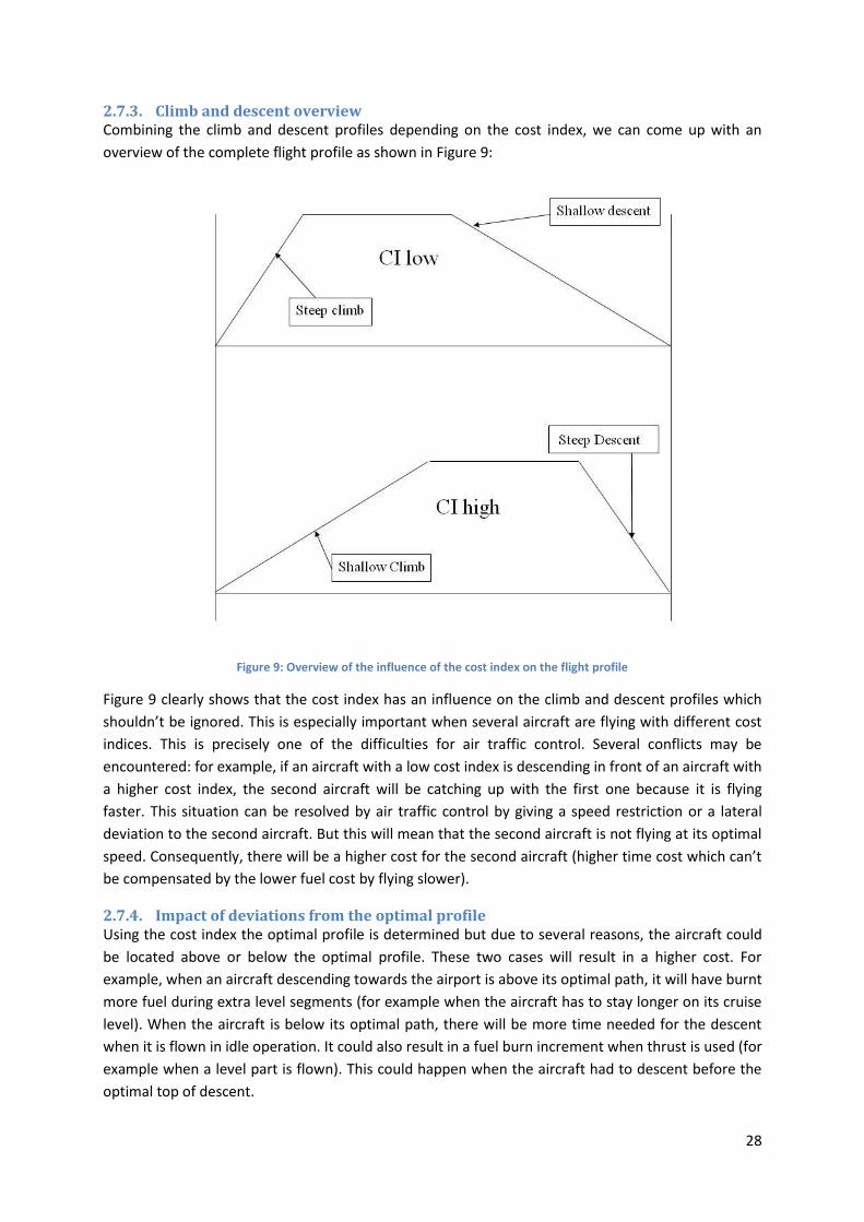
2.7.3. Climb and descent overview Combining the climb and descent profiles depending on the cost index, we can come up with an
overview of the complete flight profile as shown in Figure 9:
Figure 9: Overview of the influence of the cost index on the flight profile
Figure 9 clearly shows that the cost index has an influence on the climb and descent profiles which
shouldn’t be ignored. This is especially important when several aircraft are flying with different cost
indices. This is precisely one of the difficulties for air traffic control. Several conflicts may be
encountered: for example, if an aircraft with a low cost index is descending in front of an aircraft with
a higher cost index, the second aircraft will be catching up with the first one because it is flying
faster. This situation can be resolved by air traffic control by giving a speed restriction or a lateral
deviation to the second aircraft. But this will mean that the second aircraft is not flying at its optimal
speed. Consequently, there will be a higher cost for the second aircraft (higher time cost which can’t
be compensated by the lower fuel cost by flying slower).
2.7.4. Impact of deviations from the optimal profile Using the cost index the optimal profile is determined but due to several reasons, the aircraft could
be located above or below the optimal profile. These two cases will result in a higher cost. For
example, when an aircraft descending towards the airport is above its optimal path, it will have burnt
more fuel during extra level segments (for example when the aircraft has to stay longer on its cruise
level). When the aircraft is below its optimal path, there will be more time needed for the descent
when it is flown in idle operation. It could also result in a fuel burn increment when thrust is used (for
example when a level part is flown). This could happen when the aircraft had to descent before the
optimal top of descent.

29
2.7.5. Influence of different cost indices When all airlines are using different cost indices, all aircraft are flying at a different speed. This is very
hard for air traffic control because additional interventions are needed to keep aircraft separated.
This is for example the case when low cost airlines are flying at a very low cost index. They are
consequently flying at low speeds, which has consequences for all following aircraft. Indeed, the
aircraft flying behind a slower aircraft can get a speed restriction to maintain the required
separation. This would mean that the following aircraft can’t fly on its desired cost index anymore
which results in a higher cost. To counteract this phenomenon, the European Commission and
Eurocontrol are considering a system that improves the harmonization of the air traffic [21]. This
could be done by setting a range of cost indices that can be used by the airlines. If an airline decides
to use a cost index outside the range, a cost penalty will be given. In fact, this extra cost should then
be added as an additional factor in the calculation of the cost index. This should encourage airlines to
use a cost index in the prescribed range so that a more harmonized air traffic is obtained.

3. Software tools
3.1. BADA The Base of Aircraft Data (BADA) version 3.9 is an aircraft performance model which provides a
database of files with performance coefficients for 338 different aircraft types. These coefficients can
be used to calculate for example thrust, drag, fuel flow and reference speeds during different flight
phases. The BADA User manual provides the theoretical background and the expressions to calculate
the different performance parameters. The information in the files is intended to be used in
trajectory simulations to validate and analyse new ATM concepts or ATC procedures, for prediction
algorithms, to plan traffic flows, for environmental studies with respect to aircraft emission,...
Several types of files are provided of which the most important are:
Operations performance files: files containing the performance parameters for a particular
aircraft type.
Performance table files: files which summarize performance characteristics such as true air
speed, rates of climb and descent and fuel flow at different flight levels for a specific aircraft
type.
Performance table data: similar to the Performance table files but with more detailed
performance data.
The data which are available in the different files are intended to be used in several equations and
models which are described in [22]. The atmospheric model (see 4.1) and the total energy model (see
4.2) are the most important ones and will also be used in this work. The principle data that are used
from the files are thrust, drag and fuel flow coefficients and typical weights.
3.1.1. Drag calculation The drag is calculated using the well known relations [22]:
(3.1)
(3.2)
is the coefficient that is more commonly written as k. This notation is used to be coherent with
the BADA database.
(3.3)
3.1.2. Thrust calculation [22] Thrust determination is done depending on the phase of flight, the type of engines, the pressure
altitude h and the true airspeed V. The maximum climb and takeoff thrust is calculated as follows:

31
Jets:
(3.4)
Turboprops:
(3.5)
With: FA: Thrust (Newton) : Coefficients provided by BADA
(3.4) shows that the thrust of jet powered aircraft is assumed to be constant at a particular altitude,
so it is independent of the velocity.
In normal operations, the maximum climb power isn’t used to save on maintenance costs and extend
the engine life time. A factor is used to come up with the reduced climb power:
(3.6)
With: : Coefficient to be used in the rate of climb or descent calculation
: Coefficient provided by BADA : Maximum aircraft weight : Actual aircraft weight : Minimum aircraft weight
must then be added as a factor in the equation to calculate the rate of climb or descent.
The cruise and descent thrust is calculated using a factor provided in the data files:
(3.7)
(3.8)
There are different coefficients for the descent thrust depending on the altitude and on the
configuration of the aircraft.
3.1.3. Fuel burn calculation [22] Finally, the fuel consumption is determined by first calculating the thrust specific fuel consumption
(TSFC):
Jets:
(3.9)
Turboprops:
(3.10)
The nominal fuel flow can then be determined:
(3.11)
To determine the fuel flow during a descent with the engine in idle thrust, coefficients for the
minimum fuel flow are provided:
(3.12)
There is another coefficient for the fuel consumption in cruise:

32
(3.13)
3.2. V-PAT The V-PAT tool, previously called EFICAT tool, from Eurocontrol was conceived to analyse the
departure and arrival trajectories of aircraft. Initially the tool was designed to assess the descent
profiles and how good aircraft were adhering to a continuous descent approach. The main interest is
to determine the amount of level flight and where that level part has taken place during the arrival of
each aircraft. By analyzing the flights arriving at a particular airport, we can look for positions and
time periods where level parts are observed regularly. A similar analysis can be done for the
departing aircraft to evaluate level parts during the climb.
3.2.1. CCO analysis for Brussels Airport
3.2.1.1. Scope of the analysis In the past, descents into Brussels Airport were already examined by Belgocontrol in the B3 project
[2] but there are no figures or analyses yet for departing traffic. So as a part of this Master thesis, an
evaluation of the trajectories of the departing aircraft was made. For this, the flights which took off
from Brussels Airport in September 2012 were analysed.
3.2.1.2. Analysis parameters V-PAT allows to filter the available radar data so that only the data, in which we are interested, are
being displayed. The parameters as used during the analyses are shown in Table 1: Table 1: Overview of the V-PAT parameters
Parameter Setting
Above/Below Altitude Cut-Off 25,000 feet
Flight Level Tolerance 300 ft/min
Radius from ADEP 75NM
Last Plot Maximum Distance to ADEP 2 NM
Minimum Altitude Plot Cut-Off 0 feet
Optimum Climb Angle 3°
Shallow Climb Angle 2°
Use Shallow Angle in Algorithms No
Noise Delta Altitude #1 10,000 feet
Noise Delta Altitude #2 4,000 feet
Ignore Flights Cruise Below 5,000 feet
Minimum Level Distance Above Altitude 0 NM
Minimum Level Distance Below Altitude 0 NM
Minimum Time for Level Plots 20 seconds
The reasoning behind these settings is as follows:
Above/Below Altitude Cut-Off:
This parameter sets a vertical limit to the airspace in which the analysis is performed. Since data from
Belgocontrol are used, the analysis can only be done inside the airspace of Belgocontrol as set by the

33
agreement with Eurocontrol and Belgocontrol. This airspace goes up to FL24516 so 25,000 feet was
selected as maximum altitude for the analysis since the program allows choosing between multiples
of 1,000ft. However, it would be very interesting if the analysis could be performed without this limit.
Flight Level Tolerance:
To determine when a part of a flight is flown level, the flight level tolerance is set. When the rate of
climb between two radar plots is lower than the parameter setting, the flight is considered as flying
level between these two plots. This parameter is also used to suppress any faulty results due to small
errors of the altitude of the radar plots. The setting is retrieved in an empirical way by manually
examining some flights and varying the parameter setting.
Radius from ADEP:
For the lateral limitation of the airspace, the radius from the departure airport has to be set. The user
can choose from a list with multiples of 25NM. For Brussels Airport, 75NM is chosen because this is
the best approximation of the Belgian airspace.
Last Plot Maximum Distance to ADEP:
To be sure that the considered flights have an as complete as possible set of radar plots, this
parameter determines how far the first plot of a flight can be from the airport. If the first plot is
further away than this distance, the flight is not considered in the analysis. Since the radar data of
Belgocontrol are of good quality, a distance of 2 NM around Brussels Airport was chosen.
Minimum Altitude Plot Cut-Off:
This parameter determines at which altitude the analysis is started. The first radar plots of some
flights are at an altitude of 50 feet; so to take into account the complete climb to the maximum
extend, this altitude was set to 0 feet.
Optimum Climb Angle:
The optimum climb angle is not considered in the current study because the calculations are made
for a mix of departing aircraft with large differences in optimum climb angle. V-PAT uses the
optimum climb angle when the shallow angle algorithm is activated and for the calculation of noise
deltas. The shallow angle algorithm is not used and the noise deltas are not considered.
Shallow Climb Angle:
Default values are kept because the shallow angle algorithm is not used.
Use Shallow Angle in Algorithms:
This option allows having a correction of the results in case of radar plots with a low resolution. The
radar data provided by Belgocontrol contain one plot every 4 seconds. The resolution is very well so
there is no need to use the shallow angle algorithm.
16
FL245: Flight level 245 corresponds to an altitude of 24,500ft assuming an altimeter setting of the international standard mean sea level pressure of 1013.25hPa.

34
Noise Delta Altitude #1/#2:
Default values are kept because the noise deltas are not considered.
Ignore Flights Cruise Below:
Flights which have their cruise altitude below this parameter setting will be ignored by the analysis.
FL 50 is chosen as the minimum cruise level for the considered flights. This level is pretty low but is
used to include also some flights towards nearby airports.
Minimum Level Distance Above Altitude:
This parameter sets the amount of level flight that can be ignored above the Above/Below Altitude
Cut-Off parameter. This parameter was not used since it only influences flights that are outside the
Belgian airspace (above FL245).
Minimum Level Distance Below Altitude:
Analogous to the previous parameter, this parameter sets the amount of level flight that can be
ignored but now below the Above/Below Altitude Cut-Off parameter. To get a clear view of the
whole distance flown level, this parameter was set to zero. Care must be taken that the ground roll
or part of it or taxi plots are not considered as level flight. This has only been seen for a small amount
of flights.
Minimum Time for Level Plots:
To avoid that V-PAT considers a flight segment between 2 plots as level flight due to a limited
resolution of the radar data, every level segment of less than 20 seconds is disregarded. This setting
resulted from the assessment of several flights.
3.2.1.3. Analysis setup To analyse the departing traffic, the flights are divided according to the 4 principal exit directions:
N
E-SE
SW
WNW
These sectors are represented in Figure 10 and Figure 11 which display all flights on two
representative days: respectively 28/09/2012 with departures mainly from runways 25 and
23/09/2012 with departures from runways 07.

35
Figure 10: Exit sectors with their respective limits (departures from runways 25 within a radius of 75NM)
Figure 11: Exit sectors with their respective limits (departures from runways 07 within a radius of 75NM)
The bearing intervals for the different exit directions were determined using a scatter plot (Figure
12). A bearing is the angle between the North-South axis and the line connecting the aerodrome
reference point with the exit point. The intervals retrieved from the radar data are presented in
Table 2:

36
Table 2: Bearing intervals of the exit sectors
Exit sector Bearing interval
N 322°-48°
E-SE 65°-173°
SW 191°-249°
WNW 274°-322°
Figure 12: Scatter plot of the exit bearings
To see the difference between flights flying at daytime and at night, the analysis is also done for
these two time periods. The time period from 04:00 to 20:59 (UTC17 time) is considered being
daytime and night goes from 21:00 to 03:59. The UTC time is used since the radar data are also using
the UTC time [23]. The chosen time periods are the same as those used for the preferential runway
system at Brussels Airport.
3.2.1.4. Results of the analysis The data from V-PAT were subdivided according to their departure runway, exit sector and the
departure period of the flight (day or night). To have a global overview of the situation, first all flights
are analysed together regardless of their departure time. Then the flights during daytime and night
are analysed separately to see any differences between them. The detailed results of the analyses
can be found in Results of the climb analyses.
3.2.1.4.1. Analysis of all flights This global analysis allows having a first overview of the current situation regarding departing traffic
from Brussels Airport. In the available data, from runway 20 there are only 3 flights departing to the
North and 6 flights departing to the Southwest. Since these data are statistically irrelevant, these
flights are not considered in the analysis.
First the amount of flights that have a level part in their departure profile is examined. The average is
around 9.3% of flights with a level part, ranging from 4.3% to 19.2% depending on the exit sector and
17
UTC: Coordinated Universal Time: Standard time to which many countries define their standard time. For example, Belgium is in the time zone UTC+01:00 (in wintertime).
0
100
200
300
400
500
600
700
0 45 90 135 180 225 270 315 360

37
the departure runway. The flights departing from runway 20 have the lowest average: 4.3%. In
September 2012, runway 20 was only used due to the preferential runway use system. This system is
used to distribute the noise pollution around Brussels Airport and foresees the use of runway 20
during periods with a low amount of traffic. This can be a reason for the low average. As an example,
the horizontal and vertical profiles of the flights leaving to the East and Southeast on 14/09/2012 are
respectively shown in Figure 13 and Figure 14. The corresponding profiles of only the flights that
have a level part are depicted in Figure 15 and Figure 16. The profiles of the flights leaving to the
other exit sectors are shown in Profiles of departing traffic. The same pictures for a typical weekend
day are also given in Profiles of departing traffic. The level parts in the climb profiles are only due to
traffic separation because there are no procedures containing level-off parts. North of Brussels
Airport, departing traffic can initially climb only until FL60 because arriving traffic is flying at FL70 (a
standard separation of 1,000ft is applicable). Around 50 to 60NM east of Brussels Airport, there is a
similar conflict with aircraft going towards Brussels Airport and aircraft leaving Düsseldorf and
Cologne. These are possible reasons for the level parts in the climb profiles and they clearly show the
complexity of finding solutions to achieve the goals of SESAR (see 2.3). When one would change
something to improve a certain situation, this could have negative consequences for a lot of other
situations.
Figure 13: Horizontal profiles of the flights leaving to the East and Southeast on 14/09/2012
Figure 14: Vertical profiles of the flights leaving to the East and Southeast on 14/09/2012

38
Figure 15: Horizontal profiles of the flights with a level part leaving to the East and Southeast on 14/09/2012
Figure 16: Vertical profiles of the flights with a level part leaving to the East and Southeast on 14/09/2012
The previously mentioned percentages don’t take into account the amount of level flight which is of
course more important. When looking at the amount of level flight we see that the average distances
range from 3.7 NM to 8.4 NM depending on the runway and departure direction. The total distance
flown is 63.2NM on average which results in 6.0% to 12.8% of level flight during the climb phase. This
can have several reasons: arriving aircraft, overflying aircraft, separation rules, airspace limitations,...
Analogously, the average time of level flight is calculated: from 40 to 88 seconds over an average
total climb time of about 12 minutes. These results might be a direct consequence of the settings of
the analysis parameters. Ideally, every flight should be analysed separately to see the real situation
but this is very impractical considering the large amount of flights (9641 departing flights in
September 2012 are retrieved from the available data).
From the V-PAT data the average fuel consumption and CO2 emission is deduced. Unfortunately,
these data can’t be used to make any conclusions. For example 19.2% of the flights departing from
runway 07 to the West Northwest have a level part which is around two times more than the flights
leaving to the Southwest. Remarkably the flights to the Southwest would use some 50kg more fuel
than the ones leaving to the West Northwest. Normally, one would expect that this would be the
other way around. This is due to the way of calculating the fuel consumption in V-PAT. For this, V-PAT
uses fixed values for the fuel consumption in level, descending and climbing flight with a higher fuel
consumption in climbing flight than in level flight. V-PAT doesn’t see whether the flight has already
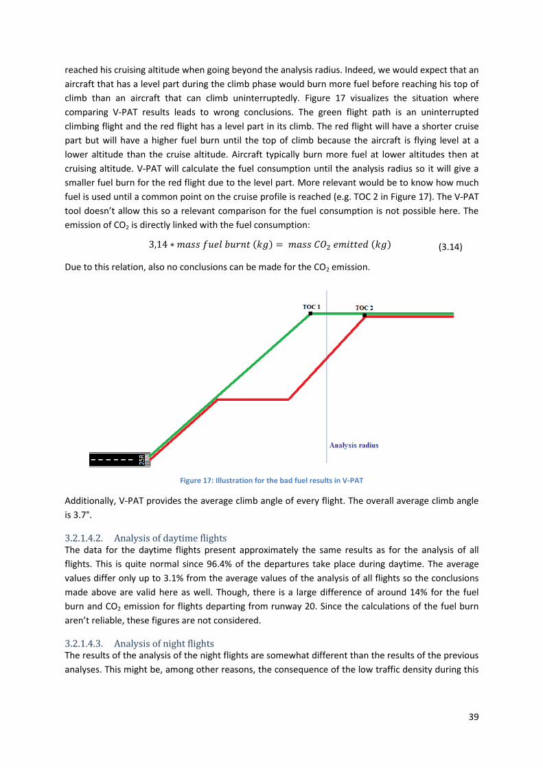
39
reached his cruising altitude when going beyond the analysis radius. Indeed, we would expect that an
aircraft that has a level part during the climb phase would burn more fuel before reaching his top of
climb than an aircraft that can climb uninterruptedly. Figure 17 visualizes the situation where
comparing V-PAT results leads to wrong conclusions. The green flight path is an uninterrupted
climbing flight and the red flight has a level part in its climb. The red flight will have a shorter cruise
part but will have a higher fuel burn until the top of climb because the aircraft is flying level at a
lower altitude than the cruise altitude. Aircraft typically burn more fuel at lower altitudes then at
cruising altitude. V-PAT will calculate the fuel consumption until the analysis radius so it will give a
smaller fuel burn for the red flight due to the level part. More relevant would be to know how much
fuel is used until a common point on the cruise profile is reached (e.g. TOC 2 in Figure 17). The V-PAT
tool doesn’t allow this so a relevant comparison for the fuel consumption is not possible here. The
emission of CO2 is directly linked with the fuel consumption:
(3.14)
Due to this relation, also no conclusions can be made for the CO2 emission.
Figure 17: Illustration for the bad fuel results in V-PAT
Additionally, V-PAT provides the average climb angle of every flight. The overall average climb angle
is 3.7°.
3.2.1.4.2. Analysis of daytime flights The data for the daytime flights present approximately the same results as for the analysis of all
flights. This is quite normal since 96.4% of the departures take place during daytime. The average
values differ only up to 3.1% from the average values of the analysis of all flights so the conclusions
made above are valid here as well. Though, there is a large difference of around 14% for the fuel
burn and CO2 emission for flights departing from runway 20. Since the calculations of the fuel burn
aren’t reliable, these figures are not considered.
3.2.1.4.3. Analysis of night flights The results of the analysis of the night flights are somewhat different than the results of the previous
analyses. This might be, among other reasons, the consequence of the low traffic density during this

40
time frame. In this analysis there are only few flights departing from runway 07 to all directions and
from runway 20 to the North and Southwest so they are not taken into account.
Very remarkable is that the amount of flights that have a level part in their climb is much lower: from
1.8% up to only 6.3% depending on their exit sector. This is around a third of the corresponding
results for all flights.
As a direct result of the lower traffic density, the total distance flown is less than during daytime (1 to
6.9 NM less). Some operational reasons might be the cause of this. Another reduction is seen for the
amount of level flight: the distance of level flight in the climb (for flights having a level part) appears
to be lower than for day flights, except for the flights leaving to the Southwest and West Northwest
from runway 25. However, there are very few flights with a level part so these longer level parts
could be statistical coincidences.
The time needed for the climb in the Brussels airspace is shortened with 0.5 to 1.5 minutes except
again for the flights leaving to the West Northwest from runway 25.
The average climb angles are similar to those of the daytime flights and as before, the results of the
fuel consumption and the CO2 emission are not analysed since they are not calculated in a consistent
way.
3.3. Flight data management tools Flight data from Thomas Cook are made available through the Fuel Efficiency tool from Aviaso [16].
This tool allows to extract specific parameters needed for a certain analysis, follow up certain
initiatives and have an overview of the fuel efficiency of the airline. The different data can be
exported in a number of graphical presentations which simplifies the assessment of the data. A
similar tool was used with the flight data of Jetairfly.

41
4. Descent and climb profiles
4.1. Atmospheric model Aircraft performance is highly depending on the atmospheric conditions in which the flight is
undertaken. Since these conditions are continuously changing, a reference situation is taken. Here
the general International Standard Atmosphere model is taken as a reference, which is also adopted
by ICAO. This standard uses a model for the temperature, pressure and density of the air. The models
used in this work are as stated in [22], [24]. The reference temperature at sea level is 15°C (T0) with a
pressure of 1013.25 hPa (P0) and an air density of 1.225kg/m³ ( ).
4.1.1. Temperature model Temperature decreases by -6.5°C/1000m or -1.98°C/1000ft in the troposphere until the tropopause
is reached, which has a standard altitude of 11,000m or 36,089ft. Above that altitude, the
temperature remains constant at -56.5°C until the stratosphere which starts at an altitude of
20,000m or 65,617ft. This altitude will never be reached by a commercial airliner so only the model
for the troposphere and tropopause are used. The following formula will be used in the troposphere:
(4.1)
Figure 18 shows the temperature evolution according to the altitude:
Figure 18: Temperature evolution in ISA conditions
4.1.2. Pressure model The pressure at a certain altitude is calculated with the assumptions that the temperature is standard
at every altitude and that air is a perfect gas. Using the aerostatic equation (4.2) and the perfect gas
equation (4.3), an equation to calculate the pressure at a particular altitude in the troposphere is
established:
(4.2)
(4.3)
(4.4)

42
(4.5)
(4.6)
(4.7)
With: = 0.0065 K/m
Above the tropopause this becomes:
(4.8)
(4.9)
(4.10)
With: = 226.15 hPa (standard pressure at 36,089ft)
= 216.69K (standard temperature at 36,089ft)
Figure 19 shows the pressure evolution with respect to the altitude:
Figure 19: Pressure evolution in ISA conditions
4.1.3. Density model Since the air is assumed to be a perfect gas, the density is calculated using the perfect gas law (4.3).
Figure 20 shows the evolution of the air density in ISA conditions:

43
Figure 20: Density evolution in ISA conditions
4.2. Governing equations for performance calculations The equations needed for the calculations are derived from the general governing equations
retrieved from [25]:
(4.11)
(4.12)
(4.13)
With: = angle between the flight path and the horizontal going through the center of gravity
= angle between the thrust vector and the flight path = sideslip angle (angle between the flight path and the airspeed vector)
= part of the bank angle between the airspeed vector and the horizontal going through the center of gravity
We assume symmetric flight so equations (4.11)-(4.13) respectively become:
(4.14)
(4.15)
(4.16)
In (4.14)-(4.16) the angle between the thrust vector and the flight path is considered to be negligible.
This angle varies between 0° and 5° so it is acceptable to neglect its impact.

44
4.3. Performance during climb The way of executing the climb phase is depending on the priorities of the aircraft operator. For
example, a climb of a military aircraft will differ significantly from the climb of a civil transport
aircraft. In the literature, generally two typical climb trajectories are described: one with a minimum
fuel burn and one with the shortest time to climb. In reality however, airlines are working with the
cost index which is an indicator of the trade-off made between the cost of time and the cost of fuel
(see 2.7). A cost index of 0 will provide a climb with minimal fuel usage while a high cost index results
in a minimum of time needed for the climb.
4.3.1. Initial developments The following equations are used to obtain an expression for the rate of climb R/C18:
(4.17)
(4.18)
We obtain using (4.14):
(4.19)
The last factor in (4.19) is called the energy share factor which specifies how much of the available
power is used for climbing during a climb procedure. The remaining part of the available power is
then used for acceleration.
These equations are developed using the forces acting on the aircraft. Since the speed and
acceleration during the climb are changing, this has to be accounted for. A different approach is
given by the concept of energy height, which considers the changes of energy as presented in [25],
[26].When considering an aircraft at a particular altitude and speed, we can determine its total
energy:
(4.20)
The specific energy is then defined as:
(4.21)
The specific energy is independent of the aircraft characteristics and is also called the energy height
he. This is the altitude that an aircraft can reach when all its kinetic energy is traded for potential
energy. The energy height as a function of the Mach number is given in Figure 21. The lines in this
figure are lines of constant energy height: 5,000ft for the lower line and 50,000ft for the upper one
with an interval of 5,000ft for the intermediate lines.
18
R/C: Rate of climb: the amount of altitude which is gained per unit of time.

45
Figure 21: Constant energy height lines with respect to the Mach number
The derivative of the energy height with respect to time is the specific (excess) power PS:
(4.22)
Considering the force equilibrium (4.14), this can further be rewritten:
(4.23)
(4.24)
(4.25)
Using (4.22), we can come up with the final expression for the specific energy:
(4.26)
This expression is used for jet aircraft. For propeller equipped aircraft, this becomes:
(4.27)
4.3.2. Time to climb From (4.22), the time needed to go from one energy height to another can be calculated:
(4.28)
(4.29)
Relation (4.29) shows that the time to climb from one energy height to another is minimized if PS is
maximal at every energy height which is passed. These points are shown on a chart presenting the

46
energy height and the specific excess power as a function of the Mach number. If PS is maximal for a
given energy height, the PS curve is tangent to that energy height curve. Connecting all of those
points will give the trajectory to climb in the least amount of time.
This procedure is applied for a typical flight climbing to an altitude of 36,000ft (FL360) and a cruise
Mach number of 0.78. This situation corresponds to an energy height of 44,867ft. A medium size jet
powered aircraft such as the Boeing 737 or the Airbus 320 with a nominal weight is taken as an
example because these types of aircraft are most commonly used at Brussels Airport. The data
needed for the calculation are taken from the BADA database.
Figure 22: Ideal climb profile with minimal time to climb
As can be seen on Figure 22, to climb in the least amount of time possible, the aircraft initially has to
accelerate at low level before climbing. Then it continues with a rather steep climb angle on a
trajectory which connects points of maximum specific excess power at every energy height. The
aircraft comes at an energy height of 44,867ft which corresponds to an altitude of 35,900ft and
M0.784. Then the aircraft finishes its climb by remaining on the same energy height, climbing to
36,000ft and decelerating to M0.78. A zoom of this final part is presented in Figure 23.

47
Figure 23: Zoom of the final part of the climb (lowest time to climb)
The initial acceleration part as proposed here is of course not feasible because this would mean that
the aircraft would fly very low for a rather long time. This would have several disadvantages: noise
pollution and high emissions above populated areas which would mean a lot more health issues and
complaints from people living in a wide range around the airport. In addition, the aircraft needs to
stay in the controlled airspace of Brussels Airport.
The time to climb can be determined numerically by integration. This is approximated by:
(4.30)
With:
(4.31)
This is applied on the example which shows that the aircraft will reach its top of climb after nearly 23
minutes, of which only 114 seconds are taken for the low level acceleration.
4.3.3. Fuel used during the climb When an airline is only interested to fly at a low cost index, so to reduce the cost of the fuel, the
trajectory with the least consumption of fuel will be preferred. To calculate the fuel used, the fuel
specific energy fS is defined:
(4.32)
The rate of weight loss is related to the fuel flow FF:
(4.33)

48
(4.34)
(4.35)
Consequently, the total fuel consumed when climbing from energy height he1 to he2 is calculated
using:
(4.36)
This shows that the fuel consumed during the climb is minimal if fS is maximum at every energy
height which is passed. The trajectory which will consume the least amount of fuel is thus the line
which connects all points where the plots of constant fS are tangent to the plots of the energy
heights.
The same example is taken as in the previous part for the minimum time to climb. Now, lines with
constant fS are plotted together with the lines of constant energy height (see Figure 24). The climb
trajectory is similar to the trajectory for minimal time to climb, except that the climb angle is slightly
steeper. This leads to the fact that the aircraft reaches its final energy height at a higher altitude then
the requested altitude. This can clearly be seen on Figure 25: the aircraft has to descent again and
accelerate further to the final altitude and speed.
Figure 24: Ideal climb profile with minimal fuel to climb

49
Figure 25: Zoom of the final part of the climb (minimum fuel to climb)
The fuel consumed during the climb is calculated similar to the calculation of the time to climb:
(4.37)
With:
(4.38)
This method gives a fuel burn for the climb of 1946kg of which 207kg of fuel is used for the level
acceleration part.
4.3.4. Current climb procedures As stated before, the ideal climb profiles are not really useful and in strong contrast with the current
climb procedures from Brussels Airport due to the noise abatement regulations. These procedures
are described in the eAIS Package of Belgocontrol [27]. There are several SIDs19 available depending
on the departure runway and the destination of the aircraft.
The prescriptions concerning the climb gradient are the following: in order to minimize noise
nuisance and to clear obstacles in the departure area, aircraft have to maintain a net climb gradient
of at least 7% until passing 3,200ft. This corresponds to a climb angle of 4°. If unable to comply, pilots
have to advise ATS accordingly when requesting start-up clearance.
In addition to all these regulations, there are general noise abatement procedures which are already
implemented in the departure procedures. These are depending on the type of propulsion as can be
seen in Table 3. The prescriptions for jet aircraft are in accordance with the ICAO-A procedure and
the more recent NADP 1 procedure for noise abatement as stated in [28], [29].
19
SID: Standard Instrument Departure: Published flight procedure for departing flights flying IFR (Instrumental Flight Rules)

50
Table 3: Noise abatement procedures for takeoff
Turbojet aircraft Propeller aircraft
From takeoff to 1,700ft Takeoff power
Takeoff flaps
Climb to V220+10 or 20kt
or as limited by body
angle.
Takeoff power
Climb at maximum gradient
compatible with safety
Speed not less than single engine
climb speed, nor higher than best
rate of climb speed.
At 1,700ft Reduce thrust to not less than
climb thrust.
Reduce power to the maximum
normal operating power (if this power
has been used for showing compliance
with the noise certification
requirements) or to the maximum
climb power.
From 1,700ft to 3,200ft Climb at V2+10 or 20kt. Climb at the maximum gradient with
reduced power, maintaining constant
speed.
At 3,200ft Accelerate smoothly to en-
route climb speed with flaps
retraction.
Accelerate smoothly to en-route climb
speed.
After consulting some airlines for their typical climb procedures, we see that the noise abatement
procedures are adhered to. When reaching 3,200ft, acceleration is performed to 250kts below
10,000ft. After that the flight accelerates to the optimum climb speed and Mach number until the
top of climb.
The switch between flying on an indicated airspeed (IAS) and flying at a specific Mach number is
done at the crossover altitude. This altitude is depending on the cost index since the cost index is
influencing the optimum climb and descent speeds. Figure 26 [18] shows the variation of the
crossover altitudes depending on the cost index value for several Airbus aircraft families.
20
V2: Takeoff safety speed. Flying at V2 ensures that the required climb gradient can be achieved in case of an engine failure during takeoff.

51
Figure 26: Dependence of the crossover altitude on the cost index for Airbus aircraft
21 [18]
We see that for the example we are using (aircraft of the size of an A320 and Boeing 737), the
crossover altitude for a cost index equal to zero is 27,000ft. For the highest cost index (100), the
crossover altitude is around 23,500ft.
Taking into account all these constraints and typical operating procedures, we can come up with an
adapted, practical climb profile (see Figure 27) for the minimum climb time. In this profile, the
reduced thrust setting is taken into account which will reduce the fuel burn and engine deterioration
and increases the time between overhaul of the engine [30]. Because there are no limitations above
3,200ft, profiles similar to the ones retrieved before could be used above 3,200ft. This would mean a
level part at 3,200ft would be flown until a speed of 250kts is reached, followed by a climb at
constant speed to 10,000ft. At that level again a level acceleration part would take place until the
point is reached where a line of constant energy height is tangent to a line of constant specific excess
power.
21
Airbus, “Getting to grips with the cost index,” Blagnac, 1998.

52
Figure 27: Adapted profile for minimal climb time with respect to noise abatement procedures
Similarly to the initial ideal profile, it is obvious that the first level part is again not so good for noise
reasons. Additionally, it could be impossible to stay in level flight at 3,200ft because the aircraft has
to be kept in the controlled airspace of Brussels Airport. Due to this, this part is replaced by a climb
with a small rate of climb as it is generally done in current operations. To determine how much
energy will be used for respectively acceleration and the increase of height, a factor is introduced.
This is the ”energy sharing factor” (a similar factor is the “kinetic energy factor”) which reflects the
sharing between the kinetic and potential energy as stated in [22], [31]. A common value for this
factor is 0.3 which means that 30% of the energy is used for climbing and 70% for acceleration. The
same factor is applied to replace the level part at FL100. This is done because the aircraft have to be
able to reach a required altitude when leaving the Belgian airspace. In addition, a level part would
not be beneficial for passenger comfort when levelling off and starting to climb again. This gives the
profile which is taken as being the reference profile (see Figure 28).

53
Figure 28: Reference profile for minimal climb time
The profile in Figure 28 results in a climb time of 23.1 minutes which is only 0.1 minutes more than
the initially proposed profile. The calculated time to climb corresponds very well with the values in
an Airbus brochure on getting to grips with the cost index [18]. Figure 29 shows the altitude of this
profile as a function of the distance from the airport:
Figure 29: Ideal climb profile for minimal time to climb as a function of the distance from the airport
The same restrictions can be applied on the profile for minimum fuel used for the climb. Taking into
account the noise abatement restrictions, the profile in Figure 30 is retrieved. In addition the last
segment of the climb is replaced by a level part because it is hazardous to have an aircraft climbing
higher than its cruise altitude and then descending again towards it. This is especially perilous when
other aircraft are flying above the considered aircraft because certain separation minima have to be
adhered to.

54
Figure 30: Adapted profile for minimal climb fuel with respect to noise abatement procedures
This climb profile would require 1967kg of fuel to get to the top of climb. Nevertheless the same
remarks are valid for the level parts so the profile is adapted to the one in Figure 31.
Figure 31: Reference profile for minimal climb fuel
Using this profile, the aircraft will use 1973kg of fuel which is 27kg more than the initial climb profile.
It may seem unusual that the additional fuel consumption is rather limited because this profile is less
convenient for fuel efficiency. However, the use of reduced thrust results in lower fuel consumption
so the loss of efficiency is somewhat compensated. The profile in Figure 31 will be used as a
reference for minimum fuel to climb. The altitude of the reference profile is plotted as a function of
the distance from the airport in Figure 32:

55
Figure 32: Ideal climb profile for minimal fuel to climb as a function of the distance from the airport
4.3.5. Comparison of the optimal climb profiles The two reference profiles are the profiles that should be flown to minimize either the fuel burn or
the climb time which correspond to a cost index of respectively zero and the maximum value. The
profile for minimum fuel will have a steeper climb profile and a lower climb speed, a shorter climb
distance and a top of climb which is closer to the airport than the profile for minimum time.
As can be seen in Table 4, the climb profile for minimum fuel also remarkably features the least
amount of time needed to fly the profile. This is because the two profiles are not ending at the same
distance from the airport. Table 4: Overview of the climb results
Cost index
Climb profile only Climb profile with cruise segment Fuel (kg) Time (min) Distance (NM) Fuel (kg) Time (min) Distance (NM)
0 1910 22.4 129.7 2007 24.3 143.5 Maximum 2010 23.1 143.5 2010 23.1 143.5
So, in order to make an adequate comparison between these two profiles, a portion of the cruise
phase has to be considered as well for the profile for minimum fuel. This is due to the fact that the
top of climb of this profile is closer to the airport than for the other profile. So, in order to compare
the profiles up to the same distance from the airport (up to the top of climb of the profile for
minimum time), a cruise segment of 5.6NM is added to the profile for minimum fuel which brings the
total level part at the end of the profile to 13.8NM. This segment takes 1.9 minutes and 97kg of fuel
to fly it.
Figure 33 presents the two profiles with the extra cruise segment:

56
Figure 33: Overlay of the two climb profiles with the extra cruise segment
The values for the minimum fuel profile (climb profile only) in Table 4 do not take the level part at
the end of the profile into account. This part is included in the extra cruise segment since the top of
climb has been reached already at that stage.
Remarkably, the results of the fuel burn and the time needed for the climb are not very different for
both profiles. There is only a difference of 3kg of fuel and 1.1 minute of climb time. Nevertheless,
these results are similar to the results in [18] which confirms the validity of the results.
Figure 33 also clearly shows a shallower climb angle for the profile for minimum time, a longer climb
distance and a top of climb further from the airport than for the minimum fuel profile which was
expected.
All the calculated values were crosschecked with calculation methods from the BADA database,
which gave almost exactly the same results as in Table 4. The difference between the results of the
two methods is always less than 1%.
The two profiles which are proposed here are the two extreme cases that consider either fuel burn
minimization or time minimization. In real life however, there will be an intermediate situation to
trade off between fuel and time costs. This means that real life cost indices will lead to profiles being
positioned between the two extreme situations. Hence the optimal profile will be located
somewhere in between the two reference profiles.
4.3.6. Comparison with flight data Thanks to the good cooperation of Thomas Cook and Jetairfly, the proposed profiles can be
compared to profiles which have been flown by their aircraft. It was very interesting to have their
data because these two airlines fly Boeing 737s and Airbus 320s which are the aircraft taken for the
calculation of the reference profiles. The data of the complete month of September 2012 was made
available by these airlines which makes it possible to test the precise reference profiles. Because the
received information is confidential, the detailed results of the comparisons can’t be published in this
work. Nevertheless, the results are as much as possible summarized hereafter.
Considering all the data of the departing flights, the average values of the relevant parameters were
determined. Table 5 presents these values together with their standard deviation.

57
Table 5: Average climb values of the flight data
Fuel (kg) Time (min) Distance (NM)
Average Standard deviation
Average Standard deviation
Average Standard deviation
Flight data 1995 115 25.8 2.9 146.9 11 The available data only contain values for the climb profile until the top of climb so no additional
cruise segment is considered as was done in the previous paragraph.
Before we can compare the values in Table 5 with the results from the reference profiles, we have to
determine how well the data from the BADA database would lend themselves to qualitative
calculations. To verify this, the parameters of the flight data are inserted in the programs made to
determine the reference profiles. That way we can compare the real data with the calculated ones. A
number of representative flights were taken for this test such that their takeoff weight was similar to
the weight used for the reference profiles. The values of the flight data and the corresponding
calculated values are summarized in Table 6:
Table 6: Comparison of the flight data with the calculated values for the climb phase
Flight data Calculated data Fuel difference Time difference Fuel (kg)
Time (min)
Fuel (kg)
Time (min)
Kg % Min %
Flight 1 2092 28.9 2524 28.8 432 22 0.1 0.3 Flight 2 2032 26.6 2388 26.5 356 18 0.1 0.6 Flight 3 2095 27.8 2519 27.6 424 21 0.2 0.6 Flight 4 2055 27.4 2438 27.3 383 18 0.1 0.2 Flight 5 2074 29.0 2580 28.8 506 25 0.2 0.7 Flight 6 1978 25.4 2300 25.3 322 16 0.1 0.4 Flight 7 2029 28.2 2471 28.1 442 22 0.1 0.6 Flight 8 2080 27.9 2451 27.8 371 19 0.1 0.2 Flight 9 1986 25.5 2266 25.5 280 13 0.0 0.1
The results from Table 6 show that the determination of the time from the calculations comes out
very satisfactory. On the other hand, the fuel calculation for all the flights considered stands too high.
On average, the fuel burn is 19% in excess to the flight data values. This means that the fuel
consumption is overestimated by roughly some 20% when using the BADA method. Hence values
calculated beforehand for the reference profiles should be adapted to have a better approximation.
The new values for the optimal profiles are shown in Table 7:
Table 7: Reference climb parameters after correction
Cost index
Climb profile only Climb profile with cruise segment Fuel (kg) Time (min) Distance (NM) Fuel (kg) Time (min) Distance (NM)
0 1605 22.4 129.7 1687 24.3 143.5 Maximum 1689 23.1 143.5 1689 23.1 143.5
Comparing the values in Table 5 with the new ones of the reference profiles in Table 7, reveals that
the amount of fuel used during the climb by the real flights is higher than the fuel for either of the
two optimal profiles. The climb time is some minutes longer which could be the result of airline

58
policy when the cost index is rather low. This means that the fuel cost is more important so the flight
time will be longer. The profiles of the flights in Table 6 are plotted next to each other and the
reference profiles in Figure 34:
Figure 34: Comparison between real flight profiles and the reference profiles
Figure 34 reveals that the top of climb of the real flight profiles is further away from the airport than
the top of climb of the reference profiles. The profiles are also less steep starting from around FL150
so the rate of climb is smaller than proposed in the reference profiles. To further investigate this, the
altitude of the real profiles is plotted with respect to the Mach number as was done for the reference
profiles (Figure 35):
Figure 35: Comparison between real flight profiles and the reference profiles
From Figure 35 we clearly see that the flights are following the initial part of the reference profiles
which is normal because this part of the profile is restricted by operational limitations. The profile
above FL100 is thus the most interesting for optimization. In this part we see that initially almost all

59
the flights are flying a profile in between the two reference profiles which as we know can be
attributed to an intermediate cost index. Unfortunately, the last parts of the climbs are not in
between the two reference profiles. This is the result of the typical climb procedure used during the
climb. As said before, the speed below FL100 is limited to 250 kIAS22. Above FL100, the aircraft speed
is controlled using the indicated air speed until reaching the crossover altitude. The preferred
indicated airspeed is determined by the cost index value. Above the crossover altitude the Autopilot
Flight System under control of the FMS will switch to Mach number which again is determined from
the cost index. During the climb the indicated airspeed and Mach number are continuously adapted
to compensate for the wind. This method is of common use but this results in a higher fuel burn as
can be seen when comparing the results of the real flights with the reference profiles from Table 5,
Table 6 and Table 7. So due to the higher speeds in the last part of the real profiles and due to the
lower rates of climb, the top of climb is further away from the airport, the fuel burn is higher and
more time is needed to reach the top of climb. Specifically, around 306 to 390 kg of extra fuel is used,
2.7 to 3.4 minutes of extra time are needed and 3.4 to 17.2NM of extra track distance until the top of
climb is flown.
The cost index of the airlines is a confidential value so we are not in a position to calculate an ideal
profile for a specific airline. Nevertheless, the parts of the real flight paths just above FL100 in Figure
35 clearly show that the two reference profiles represent the extreme values of the cost index since
the real paths are in between the references.
It might seem strange that the real flight profiles in Figure 34 are rather far away from the reference
profiles. This is mainly because the wind is not taken into account in the reference profiles. Figure 36
shows the reference profiles corrected with the average winds of the real flights. This shows that the
real flights are still not completely in between the two reference profiles but are more tending
towards them.
Figure 36: Comparison between real flight profiles and the reference profiles corrected with the average winds
According to a very experienced pilot, equivalent class aircraft (the Airbus 320 family and Boeing 737
family are considered equivalent aircraft) will climb more or less in the same way. This can be seen
22
kIAS: knots Indicated Air Speed

60
for example in Figure 35 where flight data from both the Airbus 320 and the Boeing 737 are used. So
if two or three categories of equivalent aircraft could be established, this could allow for two or three
standard climb procedures to be optimized for the specific category. These standardized climb
procedures would be sufficient to provide every aircraft with an optimized profile which would
improve overall efficiency.
The reasoning here is specifically aimed at optimizing the climb profile so the rest of the flight is not
taken into account. So, due to the many variables acting upon any flight, it might be possible that
there are other preferred climb profiles that would be offering a better overall consideration of the
complete flight. Since these variables are not all known, we limit ourselves to this study of the climb
profiles.
4.4. Performance during descent During the descent, it would be ideal to turn off the engines and glide the aircraft down to the
runway like for the Space Shuttle. This is of course impossible due to various safety constraints and
operational reasons. However, the engines can be put in idle operation which lowers the engine
power delivery to the strict minimum to supply all accessories. So in idle operation there is still some
thrust delivered but this will be limited. Nevertheless, this is to be taken into account in the
equations. To get the most out of this procedure, the aircraft’s angle of descent should be such that
the distance flown with engines in idle condition is maximum.
4.4.1. Initial developments Equations (4.14)-(4.16) remain valid and (4.14) can be rewritten to achieve the descent angle:
(4.39)
(4.40)
(4.41)
Using (4.16) we retrieve:
(4.42)
This equation enables to calculate the optimum descent angle at every moment during the descent.
4.4.2. Descent profile for minimal time to descent When an airline considers the cost of time as being the most important, the descent should be done
in the smallest amount of time possible. Equivalently, this means that the maximum cost index value
is inserted in the FMC. The FMC will then calculate an optimum descent Mach number (MACHECON)
and descent speed (IASECON). The descent above the crossover altitude is flown at the optimum
descent Mach number while the optimum descent indicated air speed is flown below this altitude
until reaching FL100. Both optimum speeds are again corrected for the wind. Below FL100, the
indicated airspeed is limited to 250kts due to air traffic control regulations. The descent profile is
only considered up to the point where the aircraft intercepts the ILS glide slope (final approach fix)
because the glide path towards the runway is then followed. In the ILS approach the necessary

61
engine power is depending on the relative position of the aircraft with respect to the glide path
because the pilot may need to add power to stay on the glide slope. Before reaching the final
approach fix, the aircraft has to decelerate to its approach speed. So, in the complete descent profile,
there are two deceleration segments: one from the optimal descent speed to 250 kIAS before
reaching FL100 and one before the final approach fix from 250 kIAS to the approach speed.
For the practical example, the same cruise parameters are taken as for the climb profiles: cruising at
FL360 and M0.78 with an aircraft of the size of an Airbus 320 or Boeing 737 with a mass of 64000kg.
A descent towards runway 25L is considered where the glide slope interception is done at 3000ft so
the descent profile will only be calculated up to that point. More details on the precise ILS procedure
can be found on the approach chart in ILS chart runway 25L.
Since we are trying to minimize the time needed for the descent, the aircraft will have to fly as fast as
possible. Nevertheless, this speed is limited. In our example, the maximum Mach number MMO23 is
M0.82 and the maximum speed VMO24 is 350 kIAS. As a safety measure, an extra 10 knots are
deduced from the maximum speed so the maximum descent speed is 340 kIAS [18]. A similar safety
margin for the maximum Mach number is taken: the Mach number is limited to MMO-0.02, so M0.8 is
the maximum Mach number [18]. The approach speed for the interception of the glide slope is taken
to be 152 kIAS [32].
The crossover altitude is adapted to comply with the aircraft mass and the speed profile which brings
the crossover altitude to 22,520ft.
Taking into account all these parameters and applying (4.42), we can come up with the trajectory
depicted in Figure 37 which displays the altitude as a function of the true air speed:
Figure 37: Ideal descent profile for minimal time to descent
The lines of constant Mach number and constant IAS are added to show the moment where a switch
is made from flying on constant Mach number to constant IAS. Figure 38 represents the same
trajectory as a function of the Mach number:
23
MMO: Maximum operating limit Mach number 24
VMO: Maximum operating limit speed (indicated airspeed)

62
Figure 38: Ideal descent profile for minimal time to descent as a function of the Mach number
Figure 39 shows the trajectory as a function of the distance from the final approach fix:
Figure 39: Ideal descent profile for minimal time to descent as a function of the distance from the final approach fix
This figure clearly shows that during the deceleration segments, the descent angle is reduced to
allow the aircraft to decelerate sufficiently. To fly this profile, the top of descent is located at 91NM
away from the final approach fix which corresponds to the values in [18]. This profile would require
15.2 minutes to reach the final approach fix and 169kg of fuel would be needed for this. The average
descent angle is determined to be -3.1°. The average rate of descent is 2170 ft/min which is well
within the allowable limits.
4.4.3. Descent profile for minimal fuel burn When the cost of fuel is most important for an airline, this will result in a cost index of 0.
Consequently, the descent speed is much lower. Indeed, because the descent is done at idle thrust

63
setting, the top of descent should be located as far away from the airport as possible. This allows to
take advantage of the idle thrust setting and to reduce the overall fuel burn to the maximum extent
possible. As a result, the FMC will determine IASECON to be the minimum descent speed (250 kIAS in
our example). MACHECON will be M0.764 as stated in [18]. Ideally, the speed below FL100 would have
to be decreased as well to further reduce the fuel burn but 250 kIAS below FL100 is maintained
because this enables ATC to provide the necessary separation more easily. This speed profile brings
the crossover altitude to 34,160ft. Due to the lower speeds, the top of descent will be further away
from the airport, the distance to descent will be longer and the descent path will be slightly
shallower than for the profile for minimum descent time.
The results of the calculations are represented in following figures. Figure 40 presents the trajectory
with respect to true air speed:
Figure 40: Ideal descent profile for minimal fuel to descent
Figure 41 and Figure 42 show the trajectory as a function of respectively the Mach number and the
distance from the final approach fix.

64
Figure 41: Ideal descent profile for minimal fuel to descent as a function of the Mach number
Figure 42: Ideal descent profile for minimal fuel to descent as a function of the distance from the final approach fix
Figure 41 shows clearly that there is only one deceleration segment now because the speed above
and below FL100 is both 250 kIAS. This will be beneficial for passenger comfort since there is no
transitional phase before FL100 with a change of descent angle as for the profile for minimum time.
The top of descent is 117 NM away from the final approach fix, which is 26NM more than for the
profile for minimum time to descent. This profile would require 226kg of fuel and 21.4 minutes to fly
it. This is 6.2 minutes more and 57kg more than the profile for minimum time. The extra time was
expected but the extra fuel not. This is due to the longer distance flown during the descent which will
be further explained in the following paragraph. The average descent angle is -2.6° which is less than
the other profile as was expected. Also the rate of descent is lower: 1540 ft/min.

65
4.4.4. Restrictions to the descent profiles As can be seen in Figure 39 and Figure 42, the descent profiles should start at quite some distance
away from the final approach fix. This would mean that the descent should be initiated outside the
Belgian airspace. The aircraft is then still under the control of a neighbouring controlling agency.
Unfortunately, the handover from the neighbouring controlling agency to the Belgian agency
(Belgocontrol) can’t happen at whatever altitude. This handover altitude is fixed and stated in the
Letters of Agreement. These documents are not published but from a variety of different sources, we
got some of these handover altitudes. Aircraft coming via Germany are handed over at FL220 to stay
below the arriving traffic of Luxembourg Airport and aircraft arriving via France are handed over at
FL240 to be below the departures from the airports of London and the arrivals of Amsterdam Airport.
We now have to determine how far the aircraft are from the airport when they are handed over to
Belgocontrol to assess what the magnitude of the impact stemming from these handover altitudes is.
For this, the flight trajectories of a number of representative flights have been plotted on a map of
Belgium (Figure 43):
Figure 43: Flight trajectories of some representative flights towards Brussels Airport (chart
25 from [27])
The trajectories on Figure 43 show that all flights coming from a particular direction are crossing the
border in the same region. Though, the trajectory flown within the Belgian airspace is not completely
the same for all flights coming from a particular direction, which has an influence on the descent
profile. This can be clearly seen for the flight coming from Germany and landing on runway 02 (the
lower flight on Figure 43) instead of on runways 25 like the other flights. Next, the vertical profiles of
the flights coming from France and Germany are shown in respectively Figure 44 and Figure 45.
25
Belgocontrol AIM, “eAIS Package Belgium and G.-D. Luxembourg,” Belgocontrol, Steenokkerzeel, 2013.

66
Figure 44: Vertical profiles of representative flights coming from France
The vertical profiles of the flights coming from France show that the handover at FL240 happens 93
to 115NM away from the final approach fix. Remarkably these flights are doing more or less good
continuous descents.
Figure 45: Vertical profiles of representative flights coming from Germany
The flights coming from Germany clearly have a level part at FL220 which is the altitude for the
handover. This is probably due to the fact that the handover happens in a region where a lot of
traffic streams are crossing each other. The most right hand profile is the one from the flight landing
on runway 02. Figure 45 confirms that this flight has a longer flight distance between the handover
and the final approach fix. The handover is done between 81 to 137NM from the final approach fix.
To come up with reference profiles, we will consider only the situation for the flights coming from
Germany because most of the flights are arriving in this way. A reference profile will be made for a
handover at FL220 with a level part of 10NM between 104 and 114 NM from the final approach fix.

67
The handover altitude is a constraint which significantly hinders the execution of an optimized
continuous descent. Nevertheless, the profile above the handover altitude can be optimized so this
part will be exactly the same as the part of the ideal profile above FL220. Figure 46 and Figure 47
show the overlay of the ideal profile and the profile adapted to the handover constraint for
respectively minimum fuel burn and minimum descent time:
Figure 46: Overlay of the ideal profile for minimum fuel burn with and without the handover constraint
Figure 47: Overlay of the ideal profile for minimum descent time with and without the handover constraint
In Figure 46 and Figure 47, two possible efficient trajectories after the handover are depicted. The
red trajectory considers that the parts of the trajectory of constant indicated air speed below the
handover altitude are flown at a constant descent angle (profile 1). The other possibility would be to
stay at the handover altitude until the ideal profile (profile 2: the green dashed profile in Figure 46

68
and Figure 47) is intercepted. This idea is based on the fact that flying at higher altitudes is more fuel
efficient. The fuel burn and descent times of these two possibilities are summarized in Table 8:
Table 8: Fuel burn and descent time for the possible trajectories
Profile 1 Profile 2
Fuel burn (kg) Descent time
(min) Fuel burn (kg)
Descent time (min)
Profile for minimum fuel
448 30.5 542 26.2
Profile for minimum time
365 24.0 453 19.2
4.4.5. Comparison of the optimal descent profiles The calculated necessary fuel for the profile with minimal fuel burn can seem rather strange in Table
8 because it’s more than the fuel needed for the profile for minimum time to descent. But to
compare these two profiles in a representative way, we will consider the descents starting from the
same distance from the final approach fix and assume that the same cruise and climb is performed
before this point. After all, it’s the overall fuel burn and descent time that is important and not only
the parameters from the descent phase. For this we will add an extra cruise segment to the profile
for minimal time. This will end at the top of descent of the profile for minimum fuel. Figure 48
clarifies this method. For clarity, only profiles number 1 are shown in Figure 48.
Figure 48: Overlay of the two profiles with the extra cruise segment
For the calculation of the fuel consumption during the cruise segment, we need to know the cruise
Mach number which is also depending on the cost index. [18] gives us the optimal cruise Mach
number as a function of the cost index and the flight level: 0.797 for the maximum cost index. The
tops of descent of the two profiles are 19.6NM apart from each other so the extra cruise segment
will have that length. Using the BADA database, the fuel used in the cruise segment is calculated to
be 133kg and 2.6 minutes are needed to fly it. The results of the fuel burn and the descent time with
the cruise segment are summarized in Table 9:

69
Table 9: Fuel burn and descent time for the possible trajectories (extra cruise segment considered)
Profile 1 Profile 2
Fuel burn (kg) Descent time
(min) Fuel burn (kg)
Descent time (min)
Profile for minimum fuel
448 30.5 542 26.2
Profile for minimum time
498 26.6 591 21.8
The results in Table 9 show that profile 1 in Figure 46 is the best for airlines flying with a cost index of
0. To the contrary, profile 2 in Figure 47 is ideal when the maximum cost index is used. These two
profiles will be used as reference profiles as from now on.
From the data in Table 9, it is clear that profile 2 for minimum time has indeed the lowest time
needed, even with the extra cruise segment. This confirms that flying at the maximum cost index
minimizes the time to fly but this has a drawback on the fuel burn. Indeed, the profile for minimum
time consumes 143kg more fuel during the complete procedure (descent and extra cruise segment).
Inversely, the profile for minimum fuel burn takes 8.7 minutes more than the profile for minimum
time.
Remarkably, the profile for minimum time is going below the profile for minimum fuel burn just
above FL100 as can be seen on Figure 48. We would rather expect that the minimum time profile
would stay above but this is due to the necessary deceleration segment for the profile for minimum
descent time, which is not present for the other profile. Obviously, the two profiles coincide below
FL100 because the same speeds are used in that part of the descent.
The two profiles considered here are the two extreme cases which can happen. When an airline is
flying at an intermediate cost index, the ideal profile will be somewhere in between the two
presented profiles. As said before, all of this is to minimize the overall costs of the flight.
As was expected, Figure 48 shows that the top of descent of the profile for minimum time is much
closer to the final approach fix, consequently the descent distance is shorter and the descent path is
slightly steeper. This is all a direct result of the higher speeds involved during this descent procedure.
4.4.6. Comparison with flight data As was done for the climb profiles in 4.3.6, the optimal descent profiles are compared to real flight
data from Thomas Cook and Jetairfly. The comparison is done analogously to the comparison of the
climb profiles. Again the flight data from September 2012 was used for this. First, the average values
of the relevant parameters were determined and these are shown in Table 10: Table 10: Average descent values of the flight data
Fuel (kg) Time (min) Distance (NM)
Average Standard deviation
Average Standard deviation
Average Standard deviation
Flight data 539 115 27.7 5.8 141.5 20.2
The values in Table 10 are considering the descent from top of descent until touchdown on the
runway so no additional cruise segment is considered as was done for the optimal profile for
minimum time.
Calculations for the descent phase are done using other coefficients from the BADA database so we
once more have to put the flight data in the programs which are used to calculate the different

70
parameters. This way, we will determine how good the estimations with the BADA database are. A
number of relevant flights with approximately the same weight at their top of descent are taken for
the verification of the calculations. Table 11 gives an overview of the real flight data and the
corresponding calculated data:
Table 11: Comparison of the flight data with the calculated values for the descent phase
Flight data Calculated data Fuel difference Time difference
Fuel (kg)
Time (min)
Fuel (kg)
Time (min)
Kg % Min %
Flight 1 448 22,6 237,9 22,1 -210,1 -47% 0,5 2% Flight 2 463 28,7 511,1 28,4 48,1 10% 0,3 1% Flight 3 509 29,7 632,4 29,4 123,4 24% 0,3 1% Flight 4 498 29,6 300,8 29,3 -197,2 -40% 0,3 1% Flight 5 501 21,7 240,9 21,7 -260,1 -52% 0,0 0% Flight 6 504 32,4 409,8 32,4 -94,2 -19% 0,0 0% Flight 7 550 30,2 316,7 30,2 -233,3 -42% 0,0 0% Flight 8 577 28,6 652,6 28,4 75,6 13% 0,2 1% Flight 9 714 34,5 738,6 34,3 24,6 3% 0,2 1%
Flight 10 680 37,5 723,2 37,5 43,2 6% 0,0 0%
The results from Table 11 show that the calculation of the descent time is rather good: the calculated
values differ on average 0.7% from the flight data. The results of the fuel calculations however differ
a lot. This is due to the fact that there are separate coefficients in BADA for the calculation of the fuel
flow in idle setting and in level flight when thrust is needed. Unfortunately, the flight data do not
allow for separating the fuel burn of the level parts and the one of the idle parts. Since we are
considering flights coming via Germany, we will take into account only the values of those flights in
Table 11 (flights 2, 3, 9 and 10). Remarkably, the other flights almost all have fuel estimations that
are lower than the real flight data values. This is probably because these flights are coming via France
without a level part during the handover. This could be an indication that the fuel burn estimation of
BADA for the idle operation is less accurate. On average, we see that the fuel burn is overestimated
by 11% for flights 2, 3, 9 and 10. So the values from Table 9 are adapted with this correction to
improve the fuel estimation. Table 12 provides the corrected values for the descent parameters:
Table 12: Reference descent parameters after correction
Reference profiles
Fuel burn (kg) Descent time
(min) Profile for
minimum fuel 407 30.5
Profile for minimum time
537 21.8
Since the values of flights coming from different directions can have quite different values for fuel
burn, descent time and flying distance, the average values of the considered flights from Germany
are calculated (Table 13):
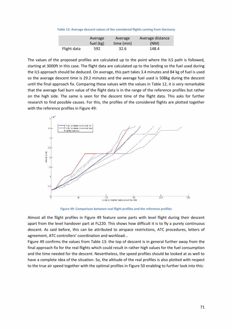
71
Table 13: Average descent values of the considered flights coming from Germany
Average fuel (kg)
Average time (min)
Average distance (NM)
Flight data 592 32.6 148.4
The values of the proposed profiles are calculated up to the point where the ILS path is followed,
starting at 3000ft in this case. The flight data are calculated up to the landing so the fuel used during
the ILS approach should be deduced. On average, this part takes 3.4 minutes and 84 kg of fuel is used
so the average descent time is 29.2 minutes and the average fuel used is 508kg during the descent
until the final approach fix. Comparing these values with the values in Table 12, it is very remarkable
that the average fuel burn value of the flight data is in the range of the reference profiles but rather
on the high side. The same is seen for the descent time of the flight data. This asks for further
research to find possible causes. For this, the profiles of the considered flights are plotted together
with the reference profiles in Figure 49:
Figure 49: Comparison between real flight profiles and the reference profiles
Almost all the flight profiles in Figure 49 feature some parts with level flight during their descent
apart from the level handover part at FL220. This shows how difficult it is to fly a purely continuous
descent. As said before, this can be attributed to airspace restrictions, ATC procedures, letters of
agreement, ATC controllers’ coordination and workload...
Figure 49 confirms the values from Table 13: the top of descent is in general further away from the
final approach fix for the real flights which could result in rather high values for the fuel consumption
and the time needed for the descent. Nevertheless, the speed profiles should be looked at as well to
have a complete idea of the situation. So, the altitude of the real profiles is also plotted with respect
to the true air speed together with the optimal profiles in Figure 50 enabling to further look into this:

72
Figure 50: Comparison between real flight profiles and the reference profiles
Figure 50 nicely displays the commonly used method for descending: first descending at a constant
Mach number until the crossover altitude, then at constant indicated air speed and finally at 250 kIAS
below FL100. Apparently, the last restriction is not adhered to by some flights. It is clear that the
flights have descended at a rather low cost index since the flights are more tending towards the
profile for minimum descent fuel. Airlines could apparently tend to use these low cost indices
because of the high fuel prices.
Coming back to the discussion of the different values of the descent fuel and time, we see however
that the speeds used during the real flights are in between speeds for the two optimal profiles. So
this is not the reason for the lower values of fuel burn and descent time for the reference profiles. In
fact, since the top of descent is earlier for the real flights, the descent will take more time. Due to this
and due to the intermediate level parts during the descent, more fuel is used in the real flights. As
explained earlier in 2.7, because the flights are not following the reference profiles, there will be a
time and/or fuel penalty which explains the high values for fuel burn and descent time for the flight
data.
4.4.7. Influence of the crossover altitude The crossover altitude is a function of the cost index (Figure 26) so since aircraft are flying at different
cost indices, their crossover altitudes are all different. This has an impact on the variation of the true
air speed during the descent. This can be seen when looking at Figure 50: aircraft flying the profile for
minimum time will achieve a much higher true air speed before reaching the crossover altitude than
aircraft flying the profile for minimum fuel.
Additionally, there are many different types of aircraft flying around which all have different speeds
during their descents. To have an idea about the variation of the crossover altitudes, the typical mix
of aircraft types in Belgium is used.
Table 14 gives an overview of the mix of aircraft types that arrived to and departed from Brussels
Airport in September 2012:
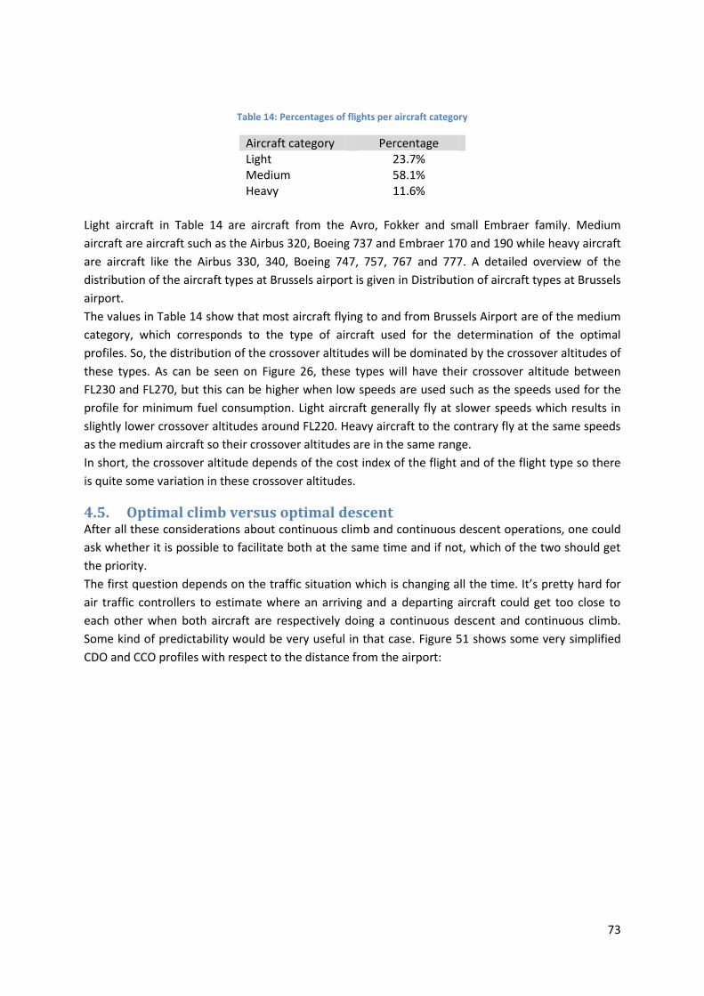
73
Table 14: Percentages of flights per aircraft category
Aircraft category Percentage Light 23.7% Medium 58.1% Heavy 11.6%
Light aircraft in Table 14 are aircraft from the Avro, Fokker and small Embraer family. Medium
aircraft are aircraft such as the Airbus 320, Boeing 737 and Embraer 170 and 190 while heavy aircraft
are aircraft like the Airbus 330, 340, Boeing 747, 757, 767 and 777. A detailed overview of the
distribution of the aircraft types at Brussels airport is given in Distribution of aircraft types at Brussels
airport.
The values in Table 14 show that most aircraft flying to and from Brussels Airport are of the medium
category, which corresponds to the type of aircraft used for the determination of the optimal
profiles. So, the distribution of the crossover altitudes will be dominated by the crossover altitudes of
these types. As can be seen on Figure 26, these types will have their crossover altitude between
FL230 and FL270, but this can be higher when low speeds are used such as the speeds used for the
profile for minimum fuel consumption. Light aircraft generally fly at slower speeds which results in
slightly lower crossover altitudes around FL220. Heavy aircraft to the contrary fly at the same speeds
as the medium aircraft so their crossover altitudes are in the same range.
In short, the crossover altitude depends of the cost index of the flight and of the flight type so there
is quite some variation in these crossover altitudes.
4.5. Optimal climb versus optimal descent After all these considerations about continuous climb and continuous descent operations, one could
ask whether it is possible to facilitate both at the same time and if not, which of the two should get
the priority.
The first question depends on the traffic situation which is changing all the time. It’s pretty hard for
air traffic controllers to estimate where an arriving and a departing aircraft could get too close to
each other when both aircraft are respectively doing a continuous descent and continuous climb.
Some kind of predictability would be very useful in that case. Figure 51 shows some very simplified
CDO and CCO profiles with respect to the distance from the airport:

74
Figure 51: Overlay of simple CDO and CCO profiles
Knowing the descent angle and the climb and descent gradient or having a good estimate of these
values, allows the air traffic controller to approximately determine where the two aircraft could get
too close to each other. This would allow the air traffic controller to intervene for example by telling
the departing aircraft to climb at a higher rate of climb to have sufficient separation between the two
aircraft. The predictability of the descent and climb profiles is one of the major issues when trying to
implement continuous descent and continuous climb procedures. So this could improve it!
When continuous climb and continuous descent operations cannot be allowed at the same time, the
question remains which of the two should get the priority to have the best overall fuel efficiency and
cost efficiency.
SAS has conducted a small analysis of this problem because there were no facts and figures available
[33]. They concluded that whenever a constraint is necessary, it will have a similar influence on
departing and arriving traffic when the constraint is known well in advance. However, when the
constraint comes all of a sudden during the approach or climb, it would be more fuel efficient to give
a constraint to a departing aircraft rather than to an arriving aircraft. Nevertheless, it is highly
depending on the type and amount of restriction and the traffic situation which aircraft should
ideally be left undisturbed.
According to Airbus [34], descent techniques have more effect on fuel and time than climb
techniques. Comparing the values of fuel burn and time for the reference profiles, we see that there
is indeed a much larger variation in the values for the descent profiles than for the climb profiles.
This shows that there are much more opportunities in the descent phase to minimize the total
operating costs than during the climb phase.
Considering all these facts, it is clearly not possible to say whether continuous climb or continuous
descent should be prioritized. This is very dependent on the traffic situation and local regulations so
it should be rather decided every time a conflict arises.

75
5. Dynamic CDO The previous part on the climb and descent profiles always considered the profile of a particular type
of aircraft. Nevertheless, aircraft are not alone in the air and they are influencing each other’s flight
paths. To go further into this, a simulation was made to determine the optimal profiles to be flown
by arriving aircraft taking into account several constraints such as airspace restrictions, other aircraft,
separation minima,... Only the descent profiles are considered in the simulation because this part of
the flight can be more optimized than the climb part as discussed before.
5.1. Concept Dynamic CDO is a simulation method to determine the best possible trajectory to descent to the
airport taking into account the actual traffic situation and the aircraft performance. For this, different
objectives can be set such as low noise, low emission, low fuel burn, least descent time or a
combination of all these. This would enable air traffic controllers to dynamically determine the
routes of arriving traffic and choose the best one for them and the pilots.
The objective of the simulation is to apply dynamic CDO in the Brussels FIR/UIR. The methodology of
[35] will be used as a basis and extended to be applied in the Brussels FIR/UIR. The simulation
enables to consider all possible variations of available airspace so a real life airspace configuration
can be used. For the testing, real life data from Belgocontrol will be used to have a realistic amount
of traffic in the simulations. Using these simulations, the possible advantages and disadvantages of
CDO implementation will be examined. Initially, only arriving traffic will be considered.
The big advantage of dynamic CDO is that predictability is increased which is good for both air traffic
control and pilots. In the future, this system can be implemented to have a real time decision making
tool for CDO.
5.2. Implementation The simulation will be performed assuming ISA conditions (see 4.1) and no wind. We will consider the airspace up to 75 NM from Brussels Airport and up to an altitude of 24,000ft. The following paragraphs illustrate the steps taken in these simulation runs.
5.2.1. Discretization of the airspace The considered airspace is discretized into 15 concentric cylinders, with the airport as centre, spaced
5NM apart. These cylinders are further discretized into 22 levels, with a separation of 1000ft. Each
level of a cylinder has artificial waypoints so that all waypoints are 1.5NM apart for safe separation.
The lower limit of the airspace is 3000ft because we consider an ILS approach to runway 25L which
has its final approach fix at 3000ft altitude. The final approach fix is assumed to be at 5NM distance
from the airport for simplification. The inner cylinder has only one level at 3000ft because the final
approach fix is located on that cylinder. The discretization of the airspace is visualized in Figure 52:

76
Figure 52: Discretized airspace around Brussels Airport
The Belgian airspace cannot be completely used by civil aviation, due to airspaces that are dedicated
to the military, amongst others. To deal with various situations of available airspace, the waypoints in
airspaces that are not available can be blocked. For example, the waypoints inside the military
training area TSA26A at the top level (24,000ft) are depicted in yellow in Figure 53:
Figure 53: Waypoints in TSA26A at 24,000ft highlighted in yellow
5.2.2. Determination of the optimal trajectory To determine whether or not an aircraft can go from one waypoint to another, the required rate of
heading change and required rate of descent between these waypoints is calculated. These values
are compared to the maximum rate of heading change and rate of descent within the aircraft
performance envelope. The maximum rates are taken from the BADA database [22]. For each
waypoint, a list of waypoints that can be reached is saved together with the time and fuel needed for

77
each of these transitions. Figure 54 shows the possible transitions for the 5 innermost rings for the
Airbus 320:
Figure 54: Possible transitions for the Airbus 320 between the 5 most inner rings
Now that all possible transitions are known, the optimal trajectory is to be searched for. Once again,
this is performed by taking into account the cost index. Unfortunately, we don’t know the cost
indices which are used by the airlines so representative values are taken. Due to calculation
capability limitations, we only consider a number of aircraft types which give a good representation
of the traffic distribution at Brussels Airport. These types and the related cost indices according to
[36] that are used in the simulation are given in Table 15: Table 15: Aircraft types with their respective cost indices for the simulation
Aircraft type Cost index
A319 12
A320 15
A321 20
A330-200 30
B737-400 15
B737-800 15
B767-300 30
DH8D 10
Embraer 145 10
Embraer 190 12
RJ1H 10
5.2.3. Multiple aircraft scenario The most interesting part of the simulation is the use of multiple aircraft. The big difficulty comes
from the different performance characteristics of different aircraft types. Since all aircraft need to be
separated, this could have a drawback on the throughput of the airspace and of the runways. So the
goal is to search for the best, conflict-free route with due respect for the time and fuel costs since we

78
are using the cost index parameter. The separation in the simulation is done by blocking waypoints
behind an aircraft for a certain time period. This time period is depending on the wake turbulence
category (WTC) of the concerned aircraft and the following aircraft [37]. Table 16 shows the
applicable horizontal separation minima for aircraft flying at the same altitude: Table 16: Standard separation minima for aircraft flying at the same altitude
WTC preceding aircraft WTC following aircraft Minimum separation
Heavy Heavy 4.0 NM
Heavy Medium 5.0 NM
Heavy Light 6.0 NM
Medium Light 5.0 NM
When aircraft aren’t flying at the same altitude, a minimum vertical separation of 1000ft is required.
For the simulation, a representative traffic situation from September 2012 is taken so that the
considered traffic is as realistic as possible. The “First come, first serve” method is used so that
aircraft are handled in the same order as they arrive at the boundary of the considered airspace.
A sequence of aircraft with a mix of light, medium and heavy aircraft has been chosen and is shown
in Table 17: Table 17: Simulation sequence (aircraft type and initiation time)
Aircraft number Aircraft type Initiation time (s)
1 RJ1H 0
2 A320 560
3 E145 712
4 A319 896
5 B738 1028
6 A321 1080
7 E190 1208
8 A320 1328
9 A332 1513
10 RJ1H 1796
11 B763 2009
The sequence in Table 17 shows a typical mix of aircraft landing at Brussels Airport and coming from
different directions.
5.3. Results Since we are mainly interested in minimizing the cost of each flight, only the fuel and time flown are
optimized taking into account the cost indices in Table 15. Table 18 shows the descent times, fuel
consumptions and the estimated total costs of the flights. The total cost is estimated using a fuel
price of 0.93 €/kg [38]. The cost of time was calculated using the cost index for every aircraft type
(equation (2.2)).

79
Table 18: Results of the simulation
Aircraft number Aircraft type Descent time
(min) Descent fuel (kg) Total cost (€)
1 RJ1H 18.4 219 375 2 A320 16.9 187 410 3 E145 18.1 121 280 4 A319 16.6 163 337 5 B738 17.4 190 419 6 A321 16.9 187 489 7 E190 18.4 172 365 8 A320 17.4 190 419 9 A332 16.6 348 788
10 RJ1H 18.4 219 375 11 B763 16.6 238 685
We clearly see that the light aircraft have a longer descent time because they are flying slower.
However, this is not a problem since the simulation takes into account the separation standards.
Nowadays, this is resolved by air traffic control giving speed and heading instructions to the aircraft.
The simulation does something similar: it looks for a trajectory which will probably not be the best
one but the second best one, third best one,... Figure 55 shows this for the first two aircraft of the
sequence:
Figure 55: Horizontal trajectories of the two first aircraft in the simulation sequence
Ideally, we would like to keep the same sequence of arriving aircraft which all follow more or less the
same flight pattern. A solution for this is that the separation could be done some time before the
aircraft start their descents. This separation could be done using tools which are being developed
[39], but this topic falls outside the scope of this work.
Another conclusion that can be made is that the separation conflicts can lead to a reduced
throughput. However, since Brussels Airport is not congested, there is no problem, which is clear
from the simulation results because we see that the aircraft arrive at approximately the same time as
they did in real life.

80
A big advantage of dynamic CDO is that it also optimizes the horizontal profile. The horizontal
profiles of simulated flights coming from France and Germany are presented over a chart of Belgium
in Figure 56:
Figure 56: Optimal trajectories of flights coming from France and Germany (chart
26 from [27]
)
When comparing these flight paths with the real flight paths which are flown nowadays, we see that
they are corresponding quite well (Figure 57). Though, the aircraft are staying at higher altitudes for
a longer time.
26
Belgocontrol AIM, “eAIS Package Belgium and G.-D. Luxembourg,” Belgocontrol, Steenokkerzeel, 2013.

81
Figure 57: Radar image from Belgocontrol highlighting the main traffic flows from France and Germany
In general, we can say that the dynamic CDO simulation is quite nice to calculate and present optimal
profiles for every arriving aircraft. So, the planning of flights by means of dynamic CDO increases
predictability but some additional tools might be necessary to really get a step closer to 4D flights.
82
6. Future perspectives The research in trajectory optimization in the SESAR context is far from being finished. What was
done in this work is just a part of the bigger picture. Ideally, the complete flight should be optimized,
from the moment the engines are started to the moment when they are shut down.
6.1. Cost reduction tool The contents of this work could be used in a cost reduction tool which incorporates the optimization
of all phases of the flight. Essentially, this would come down to building a tool which calculates the
most cost efficient cost index as in [40]. To be able to build this tool, the intense cooperation of an
airline will be necessary, bearing in mind confidentiality of cost items and figures.
The tool should be a combination of several smaller building blocks, each of them considering a
specific part of the flight (taxi in/out, take off, climb, cruise and descent).
6.1.1. Taxi in/out The taxi phase can consume quite some fuel when a lot of aircraft are scheduled to take off at almost
the same time. This means that the aircraft has to wait for its turn while the engines are running and
consuming fuel. The Wheeltug system could be a solution for this problem [41].
6.1.2. Takeoff The takeoff phase is highly controlled due to safety restrictions so that room for optimization is
limited. Nevertheless, nowadays most airlines use reduced takeoff power to reduce engine
deterioration, and hence maintenance costs and fuel burn, which helps optimizing the take off in the
process.
6.1.3. Climb and descent The main ideas of the climb and descent profiles have been examined in this work. However, a
number of additional aspects could be implemented to get even closer to reality. For example, the
average winds during the descent and climb could be taken into account because they can have a
large effect. A study of EUMETNET [42] showed that up to 165 kg per flight could be saved when the
actual wind is known more accurately and is taken into account.
On the aerodynamic side, the PERF and IDLE factors [43] could be taken into account for every
individual aircraft. The PERF factor is a corrective factor that adjusts the performance model of the
FMS to the real aircraft performance. It reflects the combined effect of engine and aerodynamic
deterioration which is inevitable over time. This factor is used in calculations to correct the fuel flow
and it has an impact on the specific range of the aircraft (the amount of mileage obtained per input
of fuel). With time this specific range could be reduced by up to 4-5%. The IDLE factor tunes the idle
rate of the FMS predictions to the real idle thrust. This is very important for the calculation of the
descent profile because it influences the optimal position of the top of descent.
The ideal profiles can be determined depending on the cost index by balancing the methods of the
specific excess power and the fuel specific energy.
6.1.4. Cruise The cruise phase is the longest part of the flight and therefore it is very important to optimize it.
Especially the wind is a critical parameter because with wind, the air distance is different from the
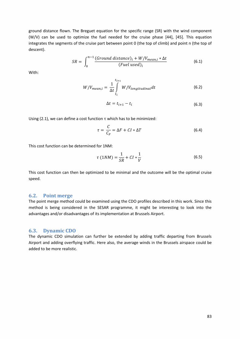
83
ground distance flown. The Breguet equation for the specific range (SR) with the wind component
(W/V) can be used to optimize the fuel needed for the cruise phase [44], [45]. This equation
integrates the segments of the cruise part between point 0 (the top of climb) and point n (the top of
descent).
(6.1)
With:
(6.2)
(6.3)
Using (2.1), we can define a cost function which has to be minimized:
(6.4)
This cost function can be determined for 1NM:
(6.5)
This cost function can then be optimized to be minimal and the outcome will be the optimal cruise
speed.
6.2. Point merge The point merge method could be examined using the CDO profiles described in this work. Since this
method is being considered in the SESAR programme, it might be interesting to look into the
advantages and/or disadvantages of its implementation at Brussels Airport.
6.3. Dynamic CDO The dynamic CDO simulation can further be extended by adding traffic departing from Brussels
Airport and adding overflying traffic. Here also, the average winds in the Brussels airspace could be
added to be more realistic.

84
7. Conclusions From the introductory texts it can be concluded that the air traffic management industry is very
eager to improve air traffic management. Nevertheless, a lot of issues remain unsolved. This is
mainly due to the fact that when changing one thing, a lot of other problems arise. This should not
hinder us however to try to improve current working methods. In this work, the focus was put on the
cost reduction of the climb and descent profiles. These were optimized considering an aircraft of the
size of the Airbus 320.
The optimization of the climb profile was done using the specific excess power and fuel specific
energy of the aircraft. Initially, the ideal profile without any constraints was calculated. Then, noise
abatement and other operational restrictions were added. The optimal profiles depend upon the
cost index, which balances between the cost of time and the cost of fuel. Optimal profiles were
calculated for two cost indices: a cost index equal to zero and a maximum value. The resulting
optimal profiles were compared to flight profiles that have been flown in real life. This revealed that,
depending on the cost index, 306 to 390kg of fuel and 2.7 to 3.4 minutes could be saved when the
optimal profiles would be flown.
The descent profiles are optimized by calculating the optimal descent angle at every moment during
the descent such that the distance flown in idle condition is maximal. Again, the ideal profiles
without constraints are calculated, after which the several restrictions were added. The most severe
restriction is the fixed handover altitude when aircraft are handed over from foreign air traffic
control to the Belgian air traffic control. This restriction is especially hindering an optimal CDO for
aircraft coming from Germany. The handover happens then over the Belgian-German border at
FL220 which means that they have to fly level for quite some time. Comparing the optimal profiles
with the flight profiles of the real flights, we see that they more or less correspond. However, the real
flights generally have to descend earlier than they would like and some intermediate level parts are
present in the descent. This is of course to be avoided because level parts ask for an increase in
thrust and consequently command more fuel burn.
Next, a closer look was taken to an air traffic control problem: should a departing aircraft be given
priority over an arriving aircraft or vice versa? The answer is highly depending on the actual traffic
situation so there is no clear-cut answer to this question. However, a simple tool to determine the
position where the two aircraft will meet and come into conflict is proposed.
The last part of this work, the dynamic CDO simulation, is tending more towards a real traffic
situation by considering multiple aircraft, different airspace constraints and separation minima for
the descending aircraft. So here not only the vertical profile is being optimized but also the horizontal
one. The Belgian airspace is considered and was discretized into a number of waypoints. All possible
trajectories, taking into account the different aircraft performance characteristics, are determined
and the most cost efficient one is selected. This is done using an estimated value for the cost index of
every aircraft. The traffic scenario was made from a mix of the typical aircraft types that are seen at
Brussels Airport. In order to have a realistic situation, the sequence and timing between aircraft
initiations was taken from real flights. Results show that optimal trajectories are almost following the
trajectories of real flights nowadays. The big advantage is that the simulation allows having better
predictability, which is one of the main hurdles for the implementation and facilitation of CDOs.
Although required research into continuous descents and continuous climbs commands a lot more
extensive work than what was performed here, most of the essential aspects of the issues at stake
were effectively addressed and examined. There is however still ample room for further research and
development around this fascinating theme.

85

86
8. References
[1] J.-J. Speyer, “Driving Flight Operations Excellence,” in 3rd Annual Flight Operations Excellence,
Marcus Evans Conference, Barcelona, 2011.
[2] B3 SESAR JU Project, “Phase two report,” 2012.
[3] Eurocontrol, “Continuous descent: A guide to implementing continuous descent,” 2011.
[4] CAA, NATS, BAA, Virgin Atlantic, British Airways, Easyjet, DfT, Mytravel, “Noise from arriving
aircraft,” 2006.
[5] ICAO, “Continuous climb operations (CCO),” 2012.
[6] SESAR Joint Undertaking, “Performance of flight trials and demonstrations validating solutions
for the reduction of CO2 emissions,” 2010.
[7] SESAR Joint Undertaking AIRE, “Reduction of emissions on the North Atlantic by the
implementation of ADS-B,” 2010.
[8] SESAR JU, “MINT project: Continuous descent approache procedure using RNP-AR,” 2009.
[9] RETA-CDA Consortium, “Reduction of emissions in terminal areas using continuous descent
approaches,” 2010.
[10] Eurocontrol, “FABs,” 2011. [Online]. Available: www.eurocontrol.int. [Accessed 21 April 2013].
[11] Eurocontrol, “Point merge: a more efficient way of sequencing arrivals,” 2011.
[12] Eurocontrol, “Point Merge successfully implemented in Dublin,” 25 January 2013. [Online].
Available: http://www.eurocontrol.int/news/point-merge-successfully-implemented-dublin.
[Accessed 25 April 2013].
[13] Eurocontrol, “CDA Map Tool,” 2010. [Online]. Available: http://extranet.eurocontrol.int.
[Accessed 10 April 2013].
[14] R. De Muynck, S. Raynaud and B. Korn, “Optimal User Forum: Session 1 - Continuous descent
approach,” 2008.
[15] J.-J. Speyer, “Getting to Grips with the Cost Index,” in 2nd Annual Flight Operations Excellence,
Marcus Evans Conference, Amsterdam, 2010.
[16] Flugwerkzeuge aviation software gmbh, “Airsavings: Cost Index Administrator Application User
Documentation,” Vienna, 2005.
[17] J.-J. Speyer, Airbus, “Are we finally Getting to Grips with the Cost Index?,” in Airline economics
seminar, Blagnac, France, 2008.

87
[18] Airbus, “Getting to grips with the cost index,” Blagnac, 1998.
[19] J.-J. Speyer, “The Cost Index as a Concept in Flight Operations,” in 3rd Annual Flight Operations
Excellence, Marcus Evans Conference, Barcelona, 2011.
[20] J.-J. Speyer, Airbus, “Airbus views on fuel economy,” in 15th Performance & Operations
conference, Puerto Vallerta, 2007.
[21] European Union, “Commission implementing regulation (EU) No 391/2013 of 3 May 2013 laying
down a common charging scheme for air navigation services,” 2013.
[22] Eurocontrol, “User manual for the base of aircraft data (BADA) revision 3.9,” Brussels, 2011.
[23] Eurocontrol, “Eurocontrol standard document for surveillance data exchange: Part 9: Category
062: SDPS Track messages,” 2009.
[24] Airbus, “Getting to grips with aircraft performance,” Airbus Industries, Blagnac, France, 2002.
[25] W. Bosschaerts, Aircraft performance, 2011.
[26] A. Mair, Aircraft performance, Cambridge: Cambridge University Press, 1992.
[27] Belgocontrol AIM, “eAIS Package Belgium and G.-D. Luxembourg,” Belgocontrol, Steenokkerzeel,
2013.
[28] P. Hopff, “Noise abatement procedures - Departures,” 2013.
[29] ICAO, “Aeroplane operating procedures,” in PANS-OPS 8168 Volume I, 2007.
[30] IATA, “IATA Fuel Book 3rd edition,” 2008.
[31] Schaufele, The elements of aircraft preliminary design, 2000.
[32] Airbus, “Flight crew operating manual,” Blagnac, 2012.
[33] Scandinavian Airlines System, Stockholm, 2011.
[34] J.-J. Speyer, Airbus, “Getting to grips with fuel economy,” Blagnac, 2004.
[35] S. Alam, M. H. Nguyen, H. A. Abbass, C. Lokan, M. Ellejmi and S. Kirby, “A Dynamic Continuous
Descent Approach Methodology for Low Noise and Emission,” 2010.
[36] J.-J. Speyer, “AirS@vings: Getting to grips with the cost index,” in 16th Performance &
Operations conference, Paris, 2009.
[37] SKYbrary, “Mitigation of Wake Turbulence Hazard,” 29 October 2012. [Online]. Available:
http://www.skybrary.aero/index.php/Mitigation_of_Wake_Turbulence_Hazard. [Accessed 7

88
May 2013].
[38] IATA, “Jet fuel price monitor,” 2013. [Online]. Available:
http://www.iata.org/publications/economics/fuel-monitor/Pages/index.aspx. [Accessed 2 June
2013].
[39] d. L. A.M.P., A. van der Eijk, M. Tielrooij and M. Mulder, “A time-space diagram based controller
support tool for continuous descent operations,” 2011.
[40] J.-J. Speyer, Airbus, “Best practices for fuel economy,” in Tunisair Fuel Economy Workshop,
Tunis, 2008.
[41] G. Dumoulin, Feasibility of electrical taxi systems / WheelTug™ to civil aircraft and to airport
types., Brussels, 2013.
[42] R. Lapsley, “Meteorology in Continuous Descent Operations,” in CDO Workshop, Eurocontrol
Headquarters Brussels, 2013.
[43] J. Ple, “Use of PERF and IDLE factors,” Airbus, 2006.
[44] J.-J. Speyer, Specificatie en Certificatie van vliegtuigen, BruFace Lecture Delivery Presentations,
Vrije Universiteit Brussel, 2013, p. 84.
[45] J.-J. Speyer, Airbus, “Fuel used method (specific range),” in 7th Performance and Operations
conference, Cancun, 1992.

9. Appendix
A. Airspace structure in the Brussels FIR
Figure 58: Chart of the airspaces in the Belgian Flight Information Region

90
B. Results of the climb analyses
RWY Directions
# Flights
% flights with level segment
Average total distance (NM) STD
Average level distance (NM)27
Average % level distance (NM)27
Average fuel burn (kg)
Average CO2 (kg)
Average total time
Average level time27
Average climb angle (°)
All flights 07 N 123 4,9%
61,0 18,4 3,7 6,0% 818,0 2576,8 0:12:10 0:00:40 3,9
E-SE 497 10,5%
65,3 12,0 7,2 11,1% 1092,6 3441,8 0:12:07 0:01:07 3,6
SW 187 9,6%
65,4 13,7 5,5 8,4% 1223,4 3853,7 0:12:35 0:00:54 3,6
WNW 125 19,2% 61,9 16,1 7,8 12,7% 1177,3 3708,6 0:12:42 0:01:22 3,6
Total 932 10,7% Overall 64,3 14,1 6,9 10,7% 1116,8 3517,8 0:12:18 0:01:06 3,6
20 N 3 0,0%
70,0 6,2 0,0 0,0% 1049,8 3306,8 0:12:16 0:00:00 3,3
E-SE 369 4,3%
62,6 11,7 3,9 6,2% 1115,2 3512,8 0:11:36 0:00:41 3,7
SW 6 0,0%
55,3 12,5 0,0 0,0% 1101,0 3468,0 0:10:39 0:00:00 4,4
WNW 0
Total 378 4,2% Overall 62,6 11,7 3,9 6,2% 1123,3 3538,5 0:11:35 0:00:41 3,7
25 N 1039 8,6%
62,4 15,5 4,3 6,8% 809,4 2549,7 0:12:18 0:00:52 3,7
E-SE 4379 9,8%
65,8 12,3 8,4 12,8% 1082,0 3408,2 0:12:06 0:01:19 3,5
SW 1679 4,7%
61,0 13,0 7,4 12,2% 1135,6 3577,2 0:11:54 0:01:28 3,9
WNW 1234 14,5% 57,3 16,0 5,8 10,1% 1164,8 3669,1 0:11:56 0:01:07 3,9
Total 8331 9,3% Overall 63,2 13,8 7,3 11,5% 1098,2 3459,4 0:12:03 0:01:14 3,7
27
Only the flights that have a level part in their climb profile were taken into account.

91
Day 07 N 122 4,9%
60,9 18,5 3,7 6,0% 816,3 2571,4 0:12:10 0:00:40 3,9
E-SE 494 10,5%
65,4 11,9 7,2 11,1% 1091,3 3437,7 0:12:08 0:01:07 3,6
SW 185 9,7%
65,5 13,8 5,5 8,4% 1217,4 3834,9 0:12:35 0:00:54 3,6
WNW 124 18,5% 61,9 16,1 8,0 12,9% 1177,3 3708,5 0:12:43 0:01:24 3,6
Total 925 10,7% Overall 64,4 14,0 6,9 10,7% 1114,7 3511,3 0:12:18 0:01:07 3,6
20 N 0
E-SE 217 5,5%
63,5 10,5 3,9 6,2% 960,7 3026,3 0:11:57 0:00:41 3,7
SW 1 0,0%
39,0 0,0 0,0 0,0% 137,1 432,0 0:09:24 0:00:00 6,0
WNW 0
Total 218 5,5% Overall 63,3 10,6 3,9 6,2% 956,9 3014,3 0:11:57 0:00:41 3,7
25 N 997 8,8%
62,5 15,6 4,3 6,9% 802,6 2528,2 0:12:21 0:00:53 3,7
E-SE 4350 9,9%
65,8 12,2 8,5 12,8% 1079,6 3400,9 0:12:06 0:01:19 3,5
SW 1622 4,8%
61,2 13,1 7,4 12,1% 1132,5 3567,3 0:11:55 0:01:27 3,9
WNW 1186 14,8% 57,5 16,1 5,8 10,0% 1174,3 3699,0 0:11:53 0:01:07 3,9
Total 8155 9,5% Overall 63,3 13,8 7,3 11,5% 1094,7 3448,5 0:12:04 0:01:14 3,7

92
Night 07 N 1 0,0%
70,0 0,0 0,0 0,0% 1027,7 3237,3 0:12:17 0:00:00 3,3
E-SE 3 0,0%
47,0 15,1 0,0 0,0% 1310,1 4126,7 0:09:27 0:00:00 4,6
SW 2 0,0%
57,5 0,5 0,0 0,0% 1774,5 5589,8 0:12:01 0:00:00 4,0
WNW 1 100,0% 65,0 0,0 4,0 6,2% 1181,1 3720,6 0:12:12 0:00:32 3,5
Total 7 14,3% Overall 55,9 13,2 4,0 7,2% 1384,0 4359,7 0:10:59 0:00:32 4,1
20 N 3 0,0%
70,0 6,2 0,0 0,0% 1049,8 3306,8 0:12:16 0:00:00 3,3
E-SE 152 2,6%
61,5 13,0 3,8 6,1% 1342,0 4227,2 0:11:05 0:00:39 3,8
SW 5 0,0%
58,6 11,1 0,0 0,0% 1293,7 4075,2 0:10:54 0:00:00 4,1
WNW 0
Total 160 2,5% Overall 61,6 12,9 3,8 6,1% 1351,9 4258,5 0:11:06 0:00:39 3,8
25 N 42 2,4%
59,2 11,8 1,0 1,7% 971,4 3059,9 0:10:49 0:00:20 4,0
E-SE 29 3,4%
63,2 13,1 4,0 6,3% 1430,5 4505,9 0:11:23 0:00:28 3,8
SW 57 1,8%
57,2 10,3 12,0 21,0% 1225,1 3859,1 0:11:09 0:02:08 4,1
WNW 48 6,3% 50,4 10,8 7,7 15,2% 930,0 2929,4 0:13:08 0:01:44 3,8
Total 176 3,4% Overall 56,8 12,1 6,7 11,7% 1277,6 4024,5 0:11:39 0:01:21 4,0

93
C. Profiles of departing traffic
a. Friday 14/09/2012
Figure 59: Horizontal profiles of the flights leaving to the North
Figure 60: Horizontal profiles of the flights with a level part leaving to the North
Figure 61: Vertical profiles of the flights leaving to the North
Figure 62: Vertical profiles of the flights with a level part leaving to the North

94
Figure 63: Horizontal profiles of the flights leaving to the Southwest
Figure 64: Horizontal profiles of the flights with a level part leaving to the Southwest
Figure 65: Vertical profiles of the flights leaving to the Southwest
Figure 66: Vertical profiles of the flights with a level part leaving to the Southwest

95
Figure 67: Horizontal profiles of the flights leaving to the West Northwest
Figure 68: Horizontal profiles of the flights with a level part leaving to the West Northwest
Figure 69: Vertical profiles of the flights leaving to the West Northwest
Figure 70: Vertical profiles of the flights with a level part leaving to the West Northwest

96
b. Sunday 23/09/2012
Figure 71: Horizontal profiles of the flights leaving to the North
Figure 72: Horizontal profiles of the flights with a level part leaving to the North
Figure 73: Vertical profiles of the flights leaving to the North
Figure 74: Vertical profiles of the flights with a level part leaving to the North

97
Figure 75: Horizontal profiles of the flights leaving to the East and Southeast
Figure 76: Horizontal profiles of the flights with a level part leaving to the East and Southeast
Figure 77: Vertical profiles of the flights leaving to the East and Southeast
Figure 78: Vertical profiles of the flights with a level part leaving to the East and Southeast

98
Figure 79: Horizontal profiles of the flights leaving to the Southwest
Figure 80: Horizontal profiles of the flights with a level part leaving to the Southwest
Figure 81: Vertical profiles of the flights leaving to the Southwest
Figure 82: Vertical profiles of the flights with a level part leaving to the Southwest

99
Figure 83: Horizontal profiles of the flights leaving to the West Northwest
Figure 84: Horizontal profiles of the flights with a level part leaving to the West Northwest
Figure 85: Vertical profiles of the flights leaving to the West Northwest
Figure 86: Vertical profiles of the flights with a level part leaving to the West Northwest
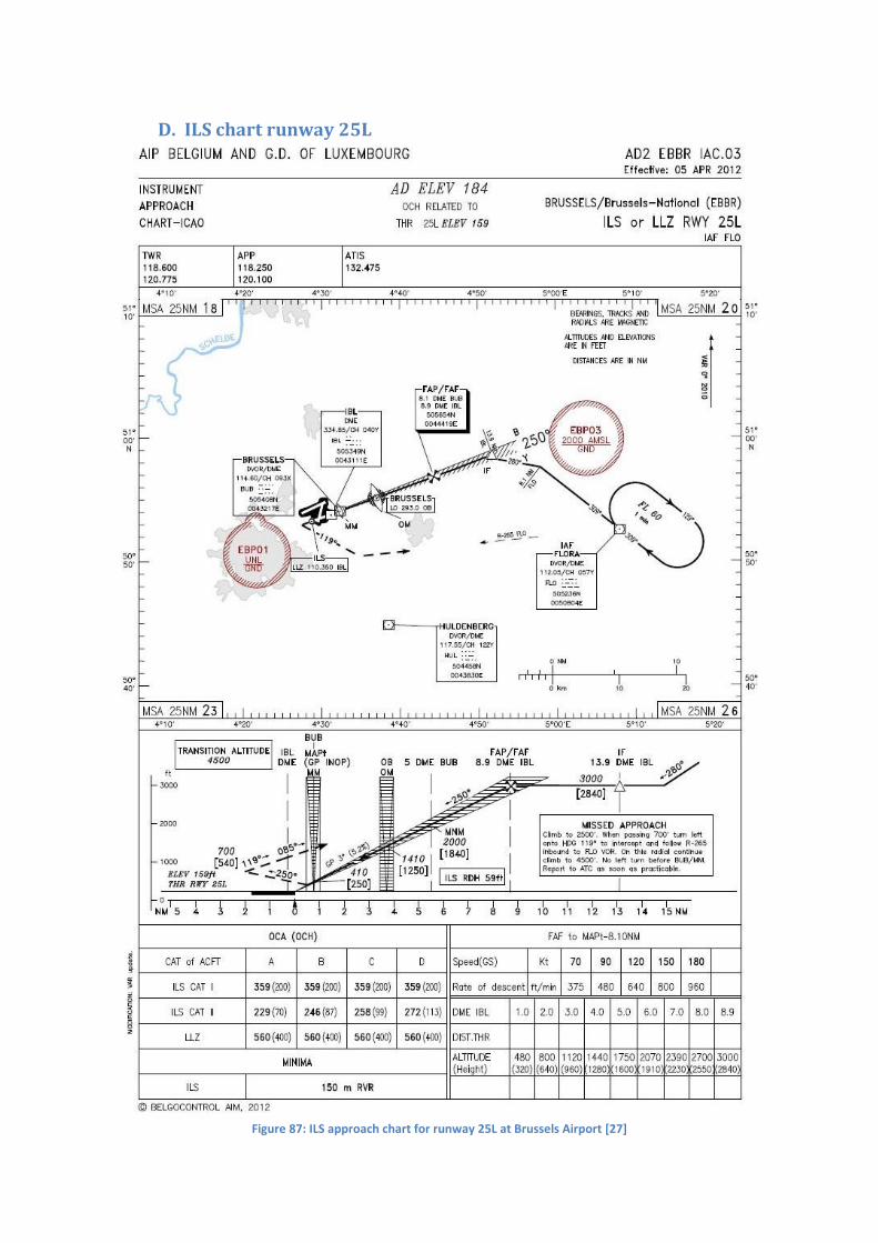
D. ILS chart runway 25L
Figure 87: ILS approach chart for runway 25L at Brussels Airport [27]

101
E. Distribution of aircraft types at Brussels airport % Departure Arrival All
% Departure Arrival All
% Departure Arrival All
A306 0,2% 0,2% 0,2%
C510 0,1% 0,1% 0,1%
LJ45 0,1% 0,1% 0,1%
A30B 0,2% 0,2% 0,2%
C525 0,1% 0,1% 0,1%
LJ60 0,1% 0,1% 0,1%
A310 0,3% 0,3% 0,3%
C550 0,2% 0,2% 0,2%
MD11 0,2% 0,2% 0,2%
A318 0,0% 0,0% 0,0%
C560 0,1% 0,1% 0,1%
MD82 0,7% 0,7% 0,7%
A319 18,4% 18,6% 18,5%
C56X 0,5% 0,5% 0,5%
MD87 0,0% 0,0% 0,0%
A320 15,4% 15,4% 15,4%
C650 0,0% 0,0% 0,0%
MU30 0,0% 0,0% 0,0%
A321 3,6% 3,6% 3,6%
C680 0,0% 0,0% 0,0%
P180 0,1% 0,1% 0,1%
A332 2,8% 2,9% 2,9%
CL30 0,0% 0,0% 0,0%
P46T 0,0% 0,0% 0,0%
A333 1,6% 1,6% 1,6%
CL60 0,2% 0,2% 0,2%
PAY3 0,0% 0,0% 0,0%
A342 0,0% 0,0% 0,0%
CRJ2 0,3% 0,3% 0,3%
PC12 0,1% 0,0% 0,0%
A343 0,1% 0,1% 0,1%
CRJ7 0,5% 0,6% 0,6%
PRM1 0,0% 0,0% 0,0%
AN28 0,0% 0,0% 0,0%
CRJ9 0,9% 0,9% 0,9%
RJ1H 10,3% 10,4% 10,3%
ATP 0,2% 0,2% 0,2%
D328 0,4% 0,4% 0,4%
RJ85 2,6% 2,6% 2,6%
B350 0,1% 0,1% 0,1%
DA42 0,0% 0,0% 0,0%
SB20 0,1% 0,1% 0,1%
B462 0,0% 0,0% 0,0%
DH8D 4,1% 4,1% 4,1%
SW4 0,1% 0,1% 0,1%
B463 0,2% 0,2% 0,2%
E120 0,0% 0,0% 0,0%
TBM7 0,0% 0,0% 0,0%
B733 2,1% 2,1% 2,1%
E135 0,9% 0,9% 0,9%
YK40 0,0% 0,0% 0,0%
B734 2,6% 2,5% 2,6%
E145 3,5% 3,6% 3,6% B735 1,6% 1,6% 1,6%
E170 0,5% 0,5% 0,5%
B736 0,6% 0,6% 0,6%
E190 4,0% 4,0% 4,0% B737 2,2% 2,2% 2,2%
E50P 0,1% 0,0% 0,1%
B738 6,2% 6,1% 6,2%
E55P 0,0% 0,0% 0,0% B739 0,1% 0,1% 0,1%
F100 0,7% 0,7% 0,7%
B742 0,1% 0,1% 0,1%
F2TH 0,2% 0,2% 0,2% B744 0,9% 0,9% 0,9%
F50 0,0% 0,0% 0,0%
B752 1,6% 1,6% 1,6%
F70 1,5% 1,5% 1,5% B762 0,2% 0,2% 0,2%
F900 0,1% 0,1% 0,1%
B763 2,4% 2,5% 2,4%
FA10 0,0% 0,0% 0,0% B772 0,7% 0,8% 0,7%
FA50 0,1% 0,1% 0,1%
B77L 0,2% 0,2% 0,2%
FA7X 0,1% 0,1% 0,1% B77W 0,1% 0,1% 0,1%
G150 0,0% 0,0% 0,0%
B788 0,0% 0,0% 0,0%
GALX 0,0% 0,0% 0,0% BE20 0,1% 0,1% 0,1%
GL5T 0,0% 0,0% 0,0%
BE30 0,0% 0,0% 0,0%
GLEX 0,1% 0,1% 0,1% BE40 0,0% 0,0% 0,0%
GLF4 0,1% 0,1% 0,1%
BE9L 0,0% 0,0% 0,0%
GLF5 0,1% 0,1% 0,1% C130 0,0% 0,0% 0,0%
H25B 0,2% 0,2% 0,2%
C25A 0,2% 0,2% 0,2%
J328 0,1% 0,1% 0,1% C25B 0,2% 0,1% 0,1%
JS32 0,1% 0,1% 0,1%
C30J 0,0% 0,0% 0,0%
JS41 0,2% 0,2% 0,2% C441 0,0% 0,0% 0,0%
LJ35 0,1% 0,1% 0,1%

F. Matlab code
a. Temperature model function result=T(h) %K T0=15+273.15; alpha=1.98; if h>36089 %ft result=216.69; else result=T0-alpha*h/1000; end end
b. Pressure model function result=P(h) %Pa P0=101325; Pt=22615; alpha=0.0065; T0=288.15; Tt=216.69; g=9.81; R=287.053;
h=h*0.3048; %m ht=11000;
if h>11000 result=Pt*exp(-g/R/Tt*(h-ht)); else result=P0*(1-alpha*h/T0)^(g/alpha/R); end end
c. Density model function result=rho(h) %kg/m³ R=287.053; result=P(h)/R/T(h); end
d. Profile for minimum climb time b=34.1; %m S=122.6; %m² AR=b^2/S; mact=72000; %kg W=mact*9.81; %N CD0=0.026984; k=0.035074; %CD2 Ctc1=158520; Ctc2=45206; Ctc3=0.11771*10^(-9); h=0:100:50000; %feet Fa=Ctc1*(1.-h/Ctc2+Ctc3.*h.^2); %N M=0:0.01:1.5; hmax=35396; %feet mmax=83000; %kg mmin=47800; %kg ES=0.3; %Energy sharing factor g=9.81;

103
Cf1=0.72987; Cf2=1236.9;
Ps=zeros(length(h),length(M)); for i=1:length(h) for j=1:length(M) V=M(j)*a(h(i)); Ps(i,j)=V*(Fa(i)/W-CD0*rho(h(i))*(V)^2*S/2/W-
W*2/S/rho(h(i))/(V)^2*k); end end Ps=Ps./0.3048.*60; %ft/min
[C,h]=contour(M,h,Ps,[0 1000 2000 3000 4000]); clabel(C,h) legend('Ps (ft/min)');
V=0:10:600; %m/s V2=V./0.3048; %feet/s he=5000:5000:50000; %feet h=zeros(length(he),length(V)); for i=1:length(he) for j=1:length(V) h(i,j,1)=he(i)-V2(j)^2/2/(9.81/0.3048); h(i,j,2)=V(j)/a(h(i,j,1)); end end hold on for i=1:length(he) plot(h(i,:,2),h(i,:,1),'b') end axis([0 1.2 0 50000]) xlabel('Mach number (-)') ylabel('Altitude (feet)')
Clmax=2.5; Vs=sqrt(2*W/rho(0)/S/Clmax);
V2=1.13*Vs; %m/s V2=V2*3.6/1.852; %kts TX=[V2 V2+20 V2+20]; TY=[35 1700 3200]; n=length(TX); Cred=0.15; Cpred=1-Cred*(mmax-mact)/(mmax-mmin); dt=1; %s
while TX(n)<250/sqrt(rho(TY(n))/1.225) h=TY(n); %ft V=TX(n)*1.852/3.6; %m/s Fa=Ctc1*(1-h/Ctc2+Ctc3*h^2); Ps=V*(Fa/W-CD0*rho(h)*(V)^2*S/2/W-W*2/S/rho(h)/(V)^2*k); %m/s dh=Ps/0.3048*ES*dt*Cpred; %ft h=h+dh; TY=[TY h]; dV=Ps*(1-ES)*9.81*dt/V; V=(V+dV)/1.852*3.6; TX=[TX V]; n=length(TX); end

104
TX=[TX 250/sqrt(rho(10000)/1.225)]; TY=[TY 10000]; n=length(TX);
while TX(n)<362 h=TY(n); %ft V=TX(n)*1.852/3.6; %m/s Fa=Ctc1*(1-h/Ctc2+Ctc3*h^2); Ps=V*(Fa/W-CD0*rho(h)*(V)^2*S/2/W-W*2/S/rho(h)/(V)^2*k); %m/s dh=Ps/0.3048*ES*dt*Cpred; %ft h=h+dh; TY=[TY h]; dV=Ps*(1-ES)*9.81*dt/V; V=(V+dV)/1.852*3.6; TX=[TX V]; n=length(TX); end
for i=1:length(TX) TX(i)=(TX(i)*1.852/3.6)/a(TY(i)); end TX=[TX 0.575 0.59 0.605 0.621 0.639 0.656 0.675 0.695 0.714 0.7375
0.76 0.784 0.78]; TY=[TY 11600 13900 16200 18470 20730 23000 25200 27450 29600 31720
33900 35900 36000]; plot(TX,TY,'k','LineWidth',2)
Wf=0; x=0; %NM t=0; %s xplot=x; Gamma=[]; Fuel=0; for i=1:length(TX)-1 h1=TY(i); h2=TY(i+1); dh=h2-h1; %ft h=(h1+h2)/2; V1=TX(i)*a(h1); V2=TX(i+1)*a(h2); dV=V2-V1; %m/s V=(V1+V2)/2; Cl=2*W/(rho(h)*(V)^2*S); Cd=CD0+k*Cl^2; Fa1=Ctc1*(1-h1/Ctc2+Ctc3*h1^2); Fa2=Ctc1*(1-h2/Ctc2+Ctc3*h2^2); Fa=(Fa1+Fa2)/2; gamma=atan((-Cd/Cl+Fa/(0.5*rho(h)*V^2*S*Cl))*1/(1+V/g*dV/dh)); Gamma=[Gamma gamma]; TSFC=Cf1*(1+V*3.6/1.852/Cf2); %kg/min/kN TSFC=TSFC/60000; %kg/s/N Ps1=V1*(Fa1/W-CD0*rho(h1)*V1^2*S/2/W-W*2/S/rho(h1)/V1^2*k); %m/s Ps2=V2*(Fa2/W-CD0*rho(h2)*V2^2*S/2/W-W*2/S/rho(h2)/V2^2*k); %m/s Psavg=0.5*(1/Ps1+1/Ps2)*0.3048; %s/ft TSFC1=Cf1*(1+V1*3.6/1.852/Cf2)/60/1000; %kg/s/N TSFC2=Cf1*(1+V2*3.6/1.852/Cf2)/60/1000; %kg/s/N fs1=Ps1/TSFC1/Fa1; %m/kg fs2=Ps2/TSFC2/Fa2; %m/kg fsavg=0.5*(1/fs1+1/fs2)*0.3048; %kg/ft he1=h1+(V1/0.3048)^2/2/9.81*0.3048; %ft

105
he2=h2+(V2/0.3048)^2/2/9.81*0.3048; %ft Wf=Wf+fsavg*(he2-he1); %kg dt=Psavg*(he2-he1); %s t=t+dt; dx=V*dt*cos(gamma); %m x=x+dx; %m xplot=[xplot x]; FF=TSFC*Fa; %kg/s Fuel=Fuel+FF*dt; %kg end t Wf Fuel
figure xplot=xplot/1852; %NM plot(xplot,TY) xlabel('Distance from the airport (NM)') ylabel('Altitude (feet)')
e. Profile for minimum climb fuel b=34.1; %m S=122.6; %m² AR=b^2/S; mact=72000; %kg W=mact*9.81; %N CD0=0.026984; k=0.035074; %CD2 Ctc1=158520; Ctc2=45206; Ctc3=0.11771*10^(-9); Cf1=0.72987; Cf2=1236.9; h=0:100:50000; %feet M=0:0.01:1.5; hmax=35396; %feet mmax=83000; %kg mmin=47800; %kg ES=0.3; %Energy sharing factor g=9.81;
Ps=zeros(length(h),length(M)); Fa=zeros(length(h),length(M)); for i=1:length(h) for j=1:length(M) Fa(i,j)=Ctc1*(1.-h(i)/Ctc2+Ctc3.*h(i).^2); %N V=M(j)*a(h(i)); Ps(i,j)=V*(Fa(i)/W-CD0*rho(h(i))*(V)^2*S/2/W-
W*2/S/rho(h(i))/(V)^2*k); %m/s end end
TSFC=zeros(length(h),length(M)); for i=1:length(h) for j=1:length(M) V=M(j)*a(h(i))*3.6/1.852; TSFC(i,j)=Cf1*(1+V/Cf2); %kg/min/kN end end

106
TSFC=TSFC/60/1000; %kg/s/N
fs=Ps./TSFC./Fa; %m/kg fs=fs./0.3048; %ft/kg
[C,h]=contour(M,h,fs,[0 5 10 15 20 25 30]); clabel(C,h) legend('fs (ft/kg)');
V=0:10:600; %m/s V2=V./0.3048; %feet/s he=5000:5000:50000; %feet h=zeros(length(he),length(V)); for i=1:length(he) for j=1:length(V) h(i,j,1)=he(i)-V2(j)^2/2/(9.81/0.3048); h(i,j,2)=V(j)/a(h(i,j,1)); end end hold on for i=1:length(he) plot(h(i,:,2),h(i,:,1),'b') end axis([0 1.2 0 50000]) xlabel('Mach number (-)') ylabel('Altitude (feet)')
Clmax=2.5; Vs=sqrt(2*W/rho(0)/S/Clmax);
V2=1.13*Vs; %m/s V2=V2*3.6/1.852; %kts TX=[V2 V2+20 V2+20]; TY=[35 1700 3200];
n=length(TX); Cred=0.15; Cpred=1-Cred*(mmax-mact)/(mmax-mmin); dt=1; %s
while TX(n)<250/sqrt(rho(TY(n))/1.225) h=TY(n); %ft V=TX(n)*1.852/3.6; %m/s Fa=Ctc1*(1-h/Ctc2+Ctc3*h^2); Ps=V*(Fa/W-CD0*rho(h)*(V)^2*S/2/W-W*2/S/rho(h)/(V)^2*k); %m/s dh=Ps/0.3048*ES*dt*Cpred; %ft h=h+dh; TY=[TY h]; dV=Ps*(1-ES)*9.81*dt/V; V=(V+dV)/1.852*3.6; TX=[TX V]; n=length(TX); end
TX=[TX 250/sqrt(rho(10000)/1.225)]; TY=[TY 10000]; n=length(TX);
while TX(n)<324 h=TY(n); %ft

107
V=TX(n)*1.852/3.6; %m/s Fa=Ctc1*(1-h/Ctc2+Ctc3*h^2); Ps=V*(Fa/W-CD0*rho(h)*(V)^2*S/2/W-W*2/S/rho(h)/(V)^2*k); %m/s dh=Ps/0.3048*ES*dt*Cpred; %ft h=h+dh; TY=[TY h]; dV=Ps*(1-ES)*9.81*dt/V; V=(V+dV)/1.852*3.6; TX=[TX V]; n=length(TX); end
for i=1:length(TX) TX(i)=(TX(i)*1.852/3.6)/a(TY(i)); end TrajectoryX=[TX 0.523 0.537 0.552 0.568 0.587 0.604 0.625 0.647 0.673
0.7 0.727 0.7475 0.78]; TrajectoryY=[TY 12670 14980 17280 19580 21850 24120 26300 28500 30560
32650 34700 36000 36000]; plot(TrajectoryX,TrajectoryY,'k','LineWidth',2)
Wf=0; x=0; %NM t=0; %s xplot=x; Gamma=[]; Fuel=0; for i=1:length(TrajectoryX)-1 h1=TrajectoryY(i); h2=TrajectoryY(i+1); dh=h2-h1; %ft h=(h1+h2)/2; M1=TrajectoryX(i); M2=TrajectoryX(i+1); V1=M1*a(h1); V2=M2*a(h2); dV=V2-V1; %m/s V=(V1+V2)/2; Cl=2*W/(rho(h)*(V)^2*S); Cd=CD0+k*Cl^2; Fa1=Ctc1*(1-h1/Ctc2+Ctc3*h1^2); Fa2=Ctc1*(1-h2/Ctc2+Ctc3*h2^2); Fa=(Fa1+Fa2)/2; gamma=atan((-Cd/Cl+Fa/(0.5*rho(h)*V^2*S*Cl))*1/(1+V/g*dV/dh)); Gamma=[Gamma gamma]; TSFC=Cf1*(1+V*3.6/1.852/Cf2); %kg/min/kN TSFC=TSFC/60000; %kg/s/N k1=round(TrajectoryY(i)/100)+1; k2=round(TrajectoryY(i+1)/100)+1; j1=round(TrajectoryX(i)*100)+1; j2=round(TrajectoryX(i+1)*100)+1; j1=int64(j1); j2=int64(j2); fs1=fs(k1,j1); %ft/kg fs2=fs(k2,j2); fsavg=0.5*(1/fs1+1/fs2); he1=h1+(V1/0.3048)^2/2/9.81*0.3048; %ft he2=h2+(V2/0.3048)^2/2/9.81*0.3048; Wf=Wf+fsavg*(he2-he1); %kg Ps1=V1*(Fa1/W-CD0*rho(h1)*V1^2*S/2/W-W*2/S/rho(h1)/V1^2*k); %m/s Ps2=V2*(Fa2/W-CD0*rho(h2)*V2^2*S/2/W-W*2/S/rho(h2)/V2^2*k);

108
Psavg=0.5*(1/Ps1+1/Ps2)*0.3048; %s/ft dt=Psavg*(he2-he1); %s t=t+dt; dx=V*dt*cos(gamma); %m x=x+dx; %m xplot=[xplot x]; FF=TSFC*Fa; %kg/s Fuel=Fuel+FF*dt; %kg end Wftotal=Wf t Fuel
figure xplot=xplot/1852; %NM plot(xplot,TrajectoryY) xlabel('Distance from the airport (NM)') ylabel('Altitude (feet)')
f. Profile for minimum descent time Mini=0.8; %MMO=0.82 --> MMO-0.02 max hini=36000; %ft Vini=340; %kIAS Vini=Vini*1.852/3.6; % m/s IAS hfinal=3000; %ft Vapp=152*sqrt(1.225/rho(hfinal)); %kIAS Vapp=Vapp*1.852/3.6; %m/s g=9.81; %m/s² Ctc1=158520; Ctc2=45206; Ctc3=0.11771*10^(-9); hpdes=29831; %ft Ctdeshigh=0.13603; Ctdeslow=0.10847; Ctdesapp=0.15749; m=64000; %kg W=m*g; %N dt=0.1; %s S=122.6; %m² Cf3=14.159; Cf4=68867; Crossoveralt=22520; %ft Crossx=[150 500]; Crossy=[Crossoveralt Crossoveralt]; Handoveralt=22000; %ft Handoverdist=104; %NM Cfcr=0.96358; Cf1=0.72987; Cf2=1236.9; CTcr=0.95;
h=hfinal; V=Vapp; M=Vapp/a(h); x=0; %NM t=0; Wf=0; Mplot=M; hplot=h; xplot=x;

109
Vplot=V; Gamma=[]; ias=0;
while h<hini if (V*sqrt(rho(h)/1.225)<(250*1.852/3.6))&&(h<10000) ES=0.3; elseif (V*sqrt(rho(h)/1.225)<Vini)&&(h>10000)&&(h<Crossoveralt) ES=0.3; elseif (h>Crossoveralt) M=Mini; V=M*a(h); ES=(1+1.4*287*(-0.0065)/2/9.81*M^2)^(-1); else ES=(1+1.4*287*(-0.0065)/2/9.81*M^2+(1+0.2*M^2)^(-
1/0.4)*((1+0.2*M^2)^(1.4/0.4)-1))^(-1); ias=1; end if (x>104*1852)&&(x<114*1852) ES=0; end if h>8000 CD0=0.026984; k=0.035074; %CD2 else CD0=0.047354; k=0.040818; %CD2 end if h>hpdes K=Ctdeshigh; elseif h>8000 K=Ctdeslow; else K=Ctdesapp; end Fa=Ctc1*(1-h/Ctc2+Ctc3*h^2)*K; %N Ps=V*(Fa/W-CD0*rho(h)*(V)^2*S/2/W-W*2/S/rho(h)/(V)^2*k); %m/s if ES==0 dV=0; else dV=(1-ES)*Ps*g*dt/V; end Cl=2*W/(rho(h)*V^2*S); Cd=CD0+k*Cl^2; dz=ES*Ps*dt; %m if (h<Handoveralt)&&(ias==1) if h<10000 gamma=-atan((10000-
h)/((10000/Handoveralt*Handoverdist*1852-x)/0.3048)); else gamma=-atan((Handoveralt-h)/((Handoverdist*1852-
x)/0.3048)); end dz=V*dt*sin(gamma); dV=(1-ES)*dz/dt/ES*g*dt/V; elseif ES==0 gamma=0; else gamma=atan((-
Cd/Cl+Fa/(0.5*rho(h)*V^2*S*Cl))*1/(1+V/g*dV/dz)); end ias=0; dx=V*dt*cos(gamma); %m x=x+dx; %m xplot=[xplot x]; V=V-dV; h=h-dz/0.3048; %ft
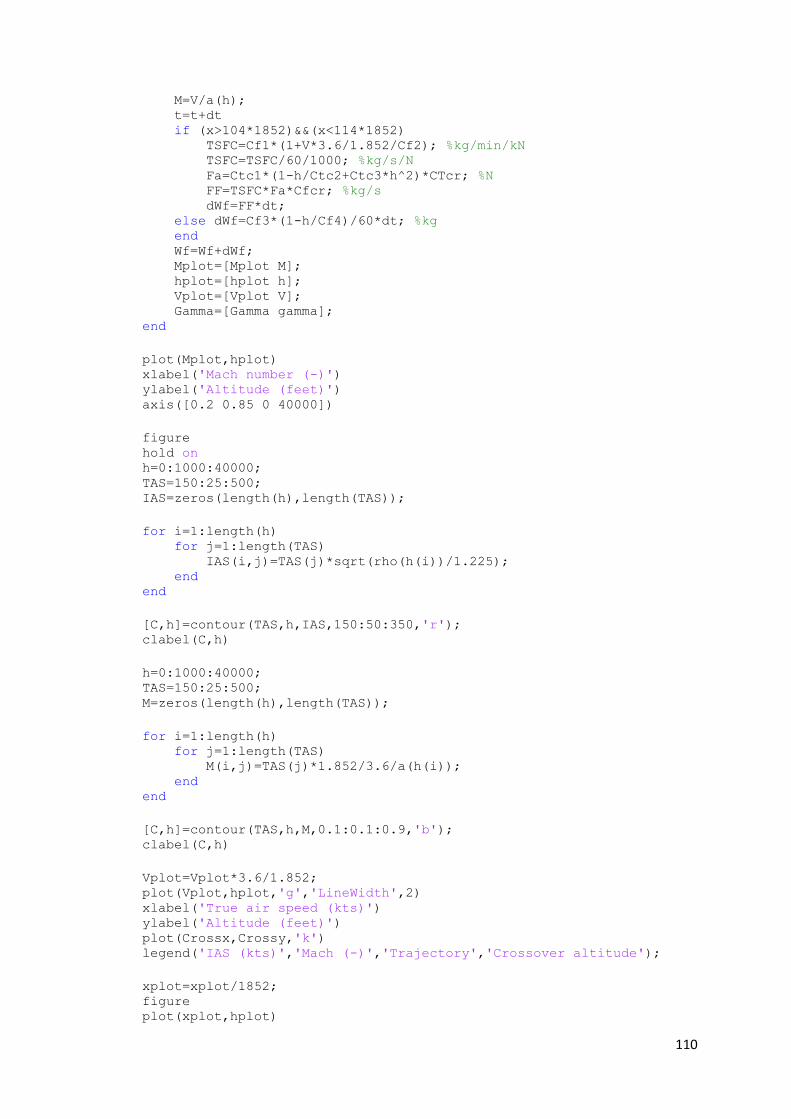
110
M=V/a(h); t=t+dt if (x>104*1852)&&(x<114*1852) TSFC=Cf1*(1+V*3.6/1.852/Cf2); %kg/min/kN TSFC=TSFC/60/1000; %kg/s/N Fa=Ctc1*(1-h/Ctc2+Ctc3*h^2)*CTcr; %N FF=TSFC*Fa*Cfcr; %kg/s dWf=FF*dt; else dWf=Cf3*(1-h/Cf4)/60*dt; %kg end Wf=Wf+dWf; Mplot=[Mplot M]; hplot=[hplot h]; Vplot=[Vplot V]; Gamma=[Gamma gamma]; end
plot(Mplot,hplot) xlabel('Mach number (-)') ylabel('Altitude (feet)') axis([0.2 0.85 0 40000])
figure hold on h=0:1000:40000; TAS=150:25:500; IAS=zeros(length(h),length(TAS));
for i=1:length(h) for j=1:length(TAS) IAS(i,j)=TAS(j)*sqrt(rho(h(i))/1.225); end end
[C,h]=contour(TAS,h,IAS,150:50:350,'r'); clabel(C,h)
h=0:1000:40000; TAS=150:25:500; M=zeros(length(h),length(TAS));
for i=1:length(h) for j=1:length(TAS) M(i,j)=TAS(j)*1.852/3.6/a(h(i)); end end
[C,h]=contour(TAS,h,M,0.1:0.1:0.9,'b'); clabel(C,h)
Vplot=Vplot*3.6/1.852; plot(Vplot,hplot,'g','LineWidth',2) xlabel('True air speed (kts)') ylabel('Altitude (feet)') plot(Crossx,Crossy,'k') legend('IAS (kts)','Mach (-)','Trajectory','Crossover altitude');
xplot=xplot/1852; figure plot(xplot,hplot)

111
xlabel('Distance from final approach fix (NM)') ylabel('Altitude (feet)')
figure Gamma=[Gamma 0]; plot(xplot,Gamma*180/pi)
t Wf
sum=0; for i=1:length(Gamma) sum=sum+Gamma(i); end avgGamma=sum/length(Gamma)*180/pi
g. Profile for minimum descent fuel Mini=0.764; %MMO=0.82 --> MMO-0.02 max hini=36000; %ft Vini=250; %kIAS Vini=Vini*1.852/3.6; % m/s IAS hfinal=3000; %ft Vapp=152*sqrt(1.225/rho(hfinal)); %kIAS Vapp=Vapp*1.852/3.6; %m/s g=9.81; %m/s² Ctc1=158520; Ctc2=45206; Ctc3=0.11771*10^(-9); hpdes=29831; %ft Ctdeshigh=0.13603; Ctdeslow=0.10847; Ctdesapp=0.15749; m=64000; %kg W=m*g; %N dt=0.1; %s S=122.6; %m² Cf3=14.159; Cf4=68867; Crossoveralt=34160; %ft Crossx=[150 500]; Crossy=[Crossoveralt Crossoveralt]; Handoveralt=22000; %ft Handoverdist=104; %NM Cfcr=0.96358; Cf1=0.72987; Cf2=1236.9; CTcr=0.95;
h=hfinal; V=Vapp; M=Vapp/a(h); x=0; %NM t=0; Wf=0; Mplot=M; hplot=h; xplot=x; Vplot=V; Gamma=[];

112
ias=0;
while h<hini if (V*sqrt(rho(h)/1.225)<(250*1.852/3.6))&&(h<10000) ES=0.3; elseif (V*sqrt(rho(h)/1.225)<Vini)&&(h>10000)&&(h<Crossoveralt) ES=0.3; elseif (h>Crossoveralt) M=Mini; V=M*a(h); ES=(1+1.4*287*(-0.0065)/2/9.81*M^2)^(-1); else ES=(1+1.4*287*(-0.0065)/2/9.81*M^2+(1+0.2*M^2)^(-
1/0.4)*((1+0.2*M^2)^(1.4/0.4)-1))^(-1); ias=1; end if (x>104*1852)&&(x<114*1852) ES=0; end if h>8000 CD0=0.026984; k=0.035074; %CD2 else CD0=0.047354; k=0.040818; %CD2 end if h>hpdes K=Ctdeshigh; elseif h>8000 K=Ctdeslow; else K=Ctdesapp; end Fa=Ctc1*(1-h/Ctc2+Ctc3*h^2)*K; %N Ps=V*(Fa/W-CD0*rho(h)*(V)^2*S/2/W-W*2/S/rho(h)/(V)^2*k); %m/s if ES==0 dV=0; else dV=(1-ES)*Ps*g*dt/V; end Cl=2*W/(rho(h)*V^2*S); Cd=CD0+k*Cl^2; dz=ES*Ps*dt; %m if (h<Handoveralt)&&(ias==1) if h<10000 gamma=-atan((10000-
h)/((10000/Handoveralt*Handoverdist*1852-x)/0.3048)); else gamma=-atan((Handoveralt-h)/((Handoverdist*1852-
x)/0.3048)); end dz=V*dt*sin(gamma); dV=(1-ES)*dz/dt/ES*g*dt/V; elseif ES==0 gamma=0; else gamma=atan((-
Cd/Cl+Fa/(0.5*rho(h)*V^2*S*Cl))*1/(1+V/g*dV/dz)); end ias=0; dx=V*dt*cos(gamma); %m x=x+dx; %m xplot=[xplot x]; V=V-dV; h=h-dz/0.3048; %ft M=V/a(h); t=t+dt

113
if (x>104*1852)&&(x<114*1852) TSFC=Cf1*(1+V*3.6/1.852/Cf2); %kg/min/kN TSFC=TSFC/60/1000; %kg/s/N Fa=Ctc1*(1-h/Ctc2+Ctc3*h^2)*CTcr; %N FF=TSFC*Fa*Cfcr; %kg/s dWf=FF*dt; else dWf=Cf3*(1-h/Cf4)/60*dt; %kg end Wf=Wf+dWf; Mplot=[Mplot M]; hplot=[hplot h]; Vplot=[Vplot V]; Gamma=[Gamma gamma]; end
plot(Mplot,hplot) xlabel('Mach number (-)') ylabel('Altitude (feet)') axis([0.2 0.85 0 40000])
figure hold on h=0:1000:40000; TAS=150:25:500; IAS=zeros(length(h),length(TAS));
for i=1:length(h) for j=1:length(TAS) IAS(i,j)=TAS(j)*sqrt(rho(h(i))/1.225); end end
[C,h]=contour(TAS,h,IAS,150:50:350,'r'); clabel(C,h)
h=0:1000:40000; TAS=150:25:500; M=zeros(length(h),length(TAS));
for i=1:length(h) for j=1:length(TAS) M(i,j)=TAS(j)*1.852/3.6/a(h(i)); end end
[C,h]=contour(TAS,h,M,0.1:0.1:0.9,'b'); clabel(C,h)
Vplot=Vplot*3.6/1.852; plot(Vplot,hplot,'g','LineWidth',2) xlabel('True air speed (kts)') ylabel('Altitude (feet)') plot(Crossx,Crossy,'k') legend('IAS (kts)','Mach (-)','Trajectory','Crossover altitude');
xplot=xplot/1852; figure plot(xplot,hplot) xlabel('Distance from final approach fix (NM)') ylabel('Altitude (feet)')

114
figure Gamma=[Gamma 0]; plot(xplot,Gamma*180/pi)
t Wf
sum=0; for i=1:length(Gamma) sum=sum+Gamma(i); end avgGamma=sum/length(Gamma)*180/pi
h. Dynamic CDO simulation %% Dynamic CDA for EBBU %% Initialization of parameters
HorSep=5; %NM VertSep=1000; %feet WedgeSep=1.5; %NM Radius=75; %NM numRings=Radius/HorSep; TopLevel=24000; %feet numLevels=(TopLevel-3000)/1000+1; % FAF at 3000ft, 5NM numWedge=zeros(numRings,1); for i=1:numRings numWedge(i)=floor(2*pi*i*HorSep/WedgeSep); end numWedgemax=floor(2*pi*Radius/WedgeSep);
%% Grid in cartesian coordinates
Gridcart=zeros(numRings,numLevels,numWedgemax,3); for i=1:numRings for j=1:numLevels for k=1:numWedge(i) theta=2*pi/numWedge(i); Gridcart(i,j,k,1)=i*HorSep*cos((k-1)*theta); %NM Gridcart(i,j,k,2)=i*HorSep*sin((k-1)*theta); %NM if i==1 Gridcart(i,1,k,3)=3000; %ft else Gridcart(i,j,k,3)=(j-1)*VertSep+3000; %ft end end end end
%% Availablility Matrix Av=Availablility(numRings,numLevels,numWedgemax,Gridcart);
%% Determining the possible transitions Path='C:\Users\Sam\Dropbox\Thesis\Matlab\Links\'; [num, txt]=xlsread('Aircraftlist.xlsx'); nbracft=max(num(:,1)); % Number of aircraft for j=1:nbracft Type(j,:)=sprintf('%s',char(txt(j+1,3))); % Types of aircraft end Starttime=num(1:nbracft,4);

115
Origin=[4.4844444 50.9013889 184*0.3048]; % Aerodrome Reference Point
[degN degE m] Pos=[num(1:nbracft,5) num(1:nbracft,6) num(1:nbracft,7)]; % Initial
position [degE degN ft] Pos(:,1)=(Pos(:,1)-Origin(1))*38; % NM Pos(:,2)=(Pos(:,2)-Origin(2))*60; % NM CI=num(:,8); Landed=0; % Number of aircraft that have reached the FAF t=2; Arracft=1; % Number of the first aircraft outside the 75 NM radius Trajectories=zeros(3,numRings,nbracft); % Trajectories of the
aircraft Trialtraj=zeros(3,numRings); Landingtime=zeros(nbracft); Timematrix=zeros(nbracft,15); Fuelmatrix=zeros(nbracft,15);
while Landed<nbracft % Calculation of the best trajectory when an aircraft arrives if Starttime(Arracft)==t Cost=1*10^30; Acft=Type(Arracft,:); Costindex=CI(Arracft); % Determination of the closest waypoint to the aircraft on
the edge of the airspace dist1=1000; %NM for i=1:numWedgemax x1=Gridcart(numRings,numLevels,i,1); y1=Gridcart(numRings,numLevels,i,2); h1=Gridcart(numRings,numLevels,i,3); if Av(numRings,numLevels,i)<t dist2=sqrt((x1-Pos(Arracft,1))^2+(y1-
Pos(Arracft,2))^2+((h1-Pos(Arracft,3))*0.3048/1852)^2); %NM if dist2<dist1 IP=[numRings numLevels i 0 0]; %Initial Point dist1=dist2; end end end
Links=load(sprintf('%s%s%s%s',Path,Acft,'\','Links'));

links1=Links.links{IP(1),IP(2),IP(3)}; for a=1:size(links1,1) Time=links1(a,4)/60; if Av(links1(a,1),links1(a,2),links1(a,3))<t Fuel=links1(a,5); Trialcost=Time*CI(Arracft)+Fuel; %kg if Trialcost<Cost links2=Links.links{links1(a,1),links1(a,2),links1(a,3)}; for b=1:size(links2,1) Time=(links1(a,4)+links2(b,4))/60; if Av(links2(b,1),links2(b,2),links2(b,3))<t+60*Time Fuel=links1(a,5)+links2(b,5); Trialcost=Time*CI(Arracft)+Fuel; %kg if Trialcost<Cost links3=Links.links{links2(b,1),links2(b,2),links2(b,3)}; for c=1:size(links3,1) Index=[a b c] Time=(links1(a,4)+links2(b,4)+links3(c,4))/60; if Av(links3(c,1),links3(c,2),links3(c,3))<t+60*Time Fuel=links1(a,5)+links2(b,5)+links3(c,5); Trialcost=Time*CI(Arracft)+Fuel; %kg if Trialcost<Cost links4=Links.links{links3(c,1),links3(c,2),links3(c,3)}; for d=1:size(links4,1) Time=(links1(a,4)+links2(b,4)+links3(c,4)+links4(d,4))/60; if Av(links4(d,1),links4(d,2),links4(d,3))<t+60*Time Fuel=links1(a,5)+links2(b,5)+links3(c,5)+links4(d,5); Trialcost=Time*CI(Arracft)+Fuel; %kg if Trialcost<Cost links5=Links.links{links4(d,1),links4(d,2),links4(d,3)}; for e=1:size(links5,1) Time=(links1(a,4)+links2(b,4)+links3(c,4)+links4(d,4)+links5(e,4))/60; if Av(links5(e,1),links5(e,2),links5(e,3))<t+60*Time Fuel=links1(a,5)+links2(b,5)+links3(c,5)+links4(d,5)+links5(e,5); Trialcost=Time*CI(Arracft)+Fuel; %kg if Trialcost<Cost links6=Links.links{links5(e,1),links5(e,2),links5(e,3)}; for f=1:size(links6,1)

117
Time=(links1(a,4)+links2(b,4)+links3(c,4)+links4(d,4)+links5(e,4)+links6(f,4))/60; if Av(links6(f,1),links6(f,2),links6(f,3))<t+60*Time Fuel=links1(a,5)+links2(b,5)+links3(c,5)+links4(d,5)+links5(e,5)+links6(f,5); Trialcost=Time*CI(Arracft)+Fuel; %kg if Trialcost<Cost links7=Links.links{links6(f,1),links6(f,2),links6(f,3)}; for g=1:size(links7,1) Time=(links1(a,4)+links2(b,4)+links3(c,4)+links4(d,4)+links5(e,4)+links6(f,4)+links7(g,4))/60; if Av(links7(g,1),links7(g,2),links7(g,3))<t+60*Time Fuel=links1(a,5)+links2(b,5)+links3(c,5)+links4(d,5)+links5(e,5)+links6(f,5)+links7(g,5); Trialcost=Time*CI(Arracft)+Fuel; %kg if Trialcost<Cost links8=Links.links{links7(g,1),links7(g,2),links7(g,3)}; for h=1:size(links8,1) Time=(links1(a,4)+links2(b,4)+links3(c,4)+links4(d,4)+links5(e,4)+links6(f,4)+
links7(g,4)+links8(h,4))/60; if Av(links8(h,1),links8(h,2),links8(h,3))<t+60*Time Fuel=links1(a,5)+links2(b,5)+links3(c,5)+links4(d,5)+links5(e,5)+links6(f,5)+
links7(g,5)+links8(h,5); Trialcost=Time*CI(Arracft)+Fuel; %kg if Trialcost<Cost links9=Links.links{links8(h,1),links8(h,2),links8(h,3)}; for i=1:size(links9,1) Time=(links1(a,4)+links2(b,4)+links3(c,4)+links4(d,4)+links5(e,4)+links6(f,4)+
links7(g,4)+links8(h,4)+links9(i,4))/60; if Av(links9(i,1),links9(i,2),links9(i,3))<t+60*Time Fuel=links1(a,5)+links2(b,5)+links3(c,5)+links4(d,5)+links5(e,5)+links6(f,5)+
links7(g,5)+links8(h,5)+links9(i,5); Trialcost=Time*CI(Arracft)+Fuel; %kg if Trialcost<Cost links10=Links.links{links9(i,1),links9(i,2),links9(i,3)}; for j=1:size(links10,1) Time=(links1(a,4)+links2(b,4)+links3(c,4)+links4(d,4)+links5(e,4)+links6(f,4)+
links7(g,4)+links8(h,4)+links9(i,4)+links10(j,4))/60; if Av(links10(j,1),links10(j,2),links10(j,3))<t+60*Time Fuel=links1(a,5)+links2(b,5)+links3(c,5)+links4(d,5)+links5(e,5)+links6(f,5)+
links7(g,5)+links8(h,5)+links9(i,5)+links10(j,5); Trialcost=Time*CI(Arracft)+Fuel; %kg if Trialcost<Cost links11=Links.links{links10(j,1),links10(j,2),links10(j,3)};

118
for k=1:size(links11,1) Time=(links1(a,4)+links2(b,4)+links3(c,4)+links4(d,4)+links5(e,4)+links6(f,4)+
links7(g,4)+links8(h,4)+links9(i,4)+links10(j,4)+links11(k,4))/60; if Av(links11(k,1),links11(k,2),links11(k,3))<t+60*Time Fuel=links1(a,5)+links2(b,5)+links3(c,5)+links4(d,5)+links5(e,5)+links6(f,5)+
links7(g,5)+links8(h,5)+links9(i,5)+links10(j,5)+links11(k,5); Trialcost=Time*CI(Arracft)+Fuel; %kg if Trialcost<Cost links12=Links.links{links11(k,1),links11(k,2),links11(k,3)}; for l=1:size(links12,1) Time=(links1(a,4)+links2(b,4)+links3(c,4)+links4(d,4)+links5(e,4)+links6(f,4)+
links7(g,4)+links8(h,4)+links9(i,4)+links10(j,4)+links11(k,4)+links12(l,4))/60; if Av(links12(l,1),links12(l,2),links12(l,3))<t+60*Time Fuel=links1(a,5)+links2(b,5)+links3(c,5)+links4(d,5)+links5(e,5)+links6(f,5)+
links7(g,5)+links8(h,5)+links9(i,5)+links10(j,5)+links11(k,5)+links12(l,5); Trialcost=Time*CI(Arracft)+Fuel; %kg if Trialcost<Cost links13=Links.links{links12(l,1),links12(l,2),links12(l,3)}; for m=1:size(links13,1) Time=(links1(a,4)+links2(b,4)+links3(c,4)+links4(d,4)+links5(e,4)+links6(f,4)+
links7(g,4)+links8(h,4)+links9(i,4)+links10(j,4)+links11(k,4)+links12(l,4)+
links13(m,4))/60; if Av(links13(m,1),links13(m,2),links13(m,3))<t+60*Time Fuel=links1(a,5)+links2(b,5)+links3(c,5)+links4(d,5)+links5(e,5)+links6(f,5)+
links7(g,5)+links8(h,5)+links9(i,5)+links10(j,5)+links11(k,5)+links12(l,5)+links13(m,5); Trialcost=Time*CI(Arracft)+Fuel; %kg if Trialcost<Cost links14=Links.links{links13(m,1),links13(m,2),links13(m,3)}; for n=1:size(links14,1) Time=(links1(a,4)+links2(b,4)+links3(c,4)+links4(d,4)+links5(e,4)+links6(f,4)+
links7(g,4)+links8(h,4)+links9(i,4)+links10(j,4)+links11(k,4)+links12(l,4)+
links13(m,4)+links14(n,4))/60; %min if Av(links14(n,1),links14(n,2),links14(n,3))<t+60*Time
Fuel=links1(a,5)+links2(b,5)+links3(c,5)+links4(d,5)+links5(e,5)+links6(f,5)+
links7(g,5)+links8(h,5)+links9(i,5)+links10(j,5)+links11(k,5)+links12(l,5)+
links13(m,5)+links14(n,5); %kg Trialcost=Time*CI(Arracft)+Fuel; %kg if Trialcost<Cost Trialtraj=[IP(1) links1(a,1) links2(b,1) links3(c,1) links4(d,1) links5(e,1)
links6(f,1) links7(g,1) links8(h,1) links9(i,1) links10(j,1) links11(k,1)

119
links12(l,1) links13(m,1) links14(n,1); IP(2) links1(a,2) links2(b,2) links3(c,2) links4(d,2) links5(e,2)
links6(f,2) links7(g,2) links8(h,2) links9(i,2) links10(j,2) links11(k,2)
links12(l,2) links13(m,2) links14(n,2); IP(3) links1(a,3) links2(b,3) links3(c,3) links4(d,3) links5(e,3)
links6(f,3) links7(g,3) links8(h,3) links9(i,3) links10(j,3) links11(k,3)
links12(l,3) links13(m,3) links14(n,3)]; Cost=Trialcost; Fuelcost=Fuel; %kg Timecost=Time; %min Timematrix(Arracft,:)=[0 links1(a,4) links2(b,4) links3(c,4) links4(d,4) links5(e,4)
links6(f,4) links7(g,4) links8(h,4) links9(i,4) links10(j,4) links11(k,4)
links12(l,4) links13(m,4) links14(n,4)]; Fuelmatrix(Arracft,:)=[0 links1(a,5) links2(b,5) links3(c,5) links4(d,5) links5(e,5)
links6(f,5) links7(g,5) links8(h,5) links9(i,5) links10(j,5) links11(k,5)
links12(l,5) links13(m,5) links14(n,5)]; end
end end clear('links14') end end end clear('links13') end end end clear('links12') end end end clear('links11') end end end clear('links10') end end end clear('links9')

120
end end end clear('links8') end end end clear('links7') end end end clear('links6') end end end clear('links5') end end end clear('links4') end end end clear('links3') end end end clear('links2') end end save(sprintf('%s%s',Path,'Trialtrajectory'),'Trialtraj'); end clear('links1')
if exist('Trialtraj','var') Trajectories(:,:,Arracft)=Trialtraj; end

121
for m=1:length(Trialtraj) Blockingtime=sum(Timematrix(Arracft,1:m)); %s Av(Trialtraj(1,m),Trialtraj(2,m),Trialtraj(3,m))=Av(Trialtraj(1,m),Trialtraj(2,m),Trialtraj(3,m))+
Blockingtime; end Av(Trialtraj(1,m),Trialtraj(2,m),Trialtraj(3,m))=Av(Trialtraj(1,m),Trialtraj(2,m),Trialtraj(3,m))+120;
Landingtime(Arracft)=t+sum(Timematrix(Arracft,:)); save(sprintf('%s%s%g%s%s',Path,'Optimal_trajectories_',Landed+1,'_',Acft),'Trajectories'); save(sprintf('%s%s%g%s%s',Path,'Fuel_burn',Landed+1,'_',Acft),'Fuelmatrix'); save(sprintf('%s%s%g%s%s',Path,'Descent_time',Landed+1,'_',Acft),'Timematrix'); save(sprintf('%s%s%g%s%s',Path,'Av_',Landed+1,'_',Acft),'Av');
Arracft=Arracft+1; Landed=Landed+1; end t=t+1; end