actually doing it: polyhedral …deloera/teaching/math114/...actually doing it: polyhedral...

ACTUALLY DOING IT:

POLYHEDRAL COMPUTATION AND ITS

APPLICATIONS

Jesus A. De LoeraDept. of Mathematics,

University of California-Davis

Davis, California, USA

[email protected]

February 24, 2010

Contents

1 PART I: WHAT THIS BOOK IS ABOUT 11.1 An exciting adventure with many hidden treasures... . . . . . . . 21.2 The Rest of this Book . . . . . . . . . . . . . . . . . . . . . . . . 14

2 PART II: Basics of Polyhedral Geometry 172.1 Polyhedral Notions . . . . . . . . . . . . . . . . . . . . . . . . . . 172.2 The characteristic features of Polyhedra . . . . . . . . . . . . . . 20

2.2.1 Equivalent representations of polyhedra, dimension andextreme points . . . . . . . . . . . . . . . . . . . . . . . . 21

2.3 Weyl-Minkowski and Polarity . . . . . . . . . . . . . . . . . . . . 23

3 PART III: Fourier-Motzkin Elimination and its Applications 273.1 Feasibility of Polyhedra and Facet-Vertex representability . . . . 27

3.1.1 Solving Systems of Linear Inequalities in Practice . . . . . 273.1.2 Fourier-Motzkin Elimination and Farkas Lemma . . . . . 303.1.3 The Face Poset of a Polytope . . . . . . . . . . . . . . . . 353.1.4 Polar Polytopes and Duality of Face Posets . . . . . . . . 36

4 PART IV: MORE TOPICS 414.1 Weyl-Minkowski again . . . . . . . . . . . . . . . . . . . . . . . . 41

4.1.1 Cones . . . . . . . . . . . . . . . . . . . . . . . . . . . . . 424.1.2 The Double Description Method . . . . . . . . . . . . . . 434.1.3 The Simplex Method and its relatives . . . . . . . . . . . 454.1.4 The Chirotope of a Point Set . . . . . . . . . . . . . . . . 534.1.5 Convex Hulls and Reverse-Search Enumeration . . . . . . 53

4.2 Visualization of Polytopes . . . . . . . . . . . . . . . . . . . . . . 554.2.1 Schlegel diagrams . . . . . . . . . . . . . . . . . . . . . . . 554.2.2 Slices and Projections . . . . . . . . . . . . . . . . . . . . 554.2.3 Nets and Unfoldings . . . . . . . . . . . . . . . . . . . . . 554.2.4 Gale Diagrams . . . . . . . . . . . . . . . . . . . . . . . . 55

4.3 Triangulations and Subdivisions . . . . . . . . . . . . . . . . . . . 554.4 Volumes and Integration over Polyhedra . . . . . . . . . . . . . . 554.5 Counting faces . . . . . . . . . . . . . . . . . . . . . . . . . . . . 55

4.5.1 Euler’s equation . . . . . . . . . . . . . . . . . . . . . . . 55

i

ii CONTENTS

4.5.2 Dehn-Sommerville Equations . . . . . . . . . . . . . . . . 554.5.3 Upper bound Theorem . . . . . . . . . . . . . . . . . . . . 554.5.4 Neighborly Polytopes . . . . . . . . . . . . . . . . . . . . 55

4.6 Graphs of Polytopes . . . . . . . . . . . . . . . . . . . . . . . . . 554.6.1 Steinitz’s theorem: 3-Polytopes . . . . . . . . . . . . . . . 554.6.2 Eberhard’s theorem . . . . . . . . . . . . . . . . . . . . . 554.6.3 Map coloring and polyhedra . . . . . . . . . . . . . . . . . 554.6.4 Paths and diameters . . . . . . . . . . . . . . . . . . . . . 554.6.5 Balinski’s theorem . . . . . . . . . . . . . . . . . . . . . . 55

4.7 Lattices and Polyhedra . . . . . . . . . . . . . . . . . . . . . . . . 554.7.1 Hilbert Bases . . . . . . . . . . . . . . . . . . . . . . . . . 554.7.2 Lattices and reduced bases . . . . . . . . . . . . . . . . . 554.7.3 Minkowski’s theorem . . . . . . . . . . . . . . . . . . . . . 554.7.4 Barvinok’s Algorithm . . . . . . . . . . . . . . . . . . . . 55

4.8 Containment Problems . . . . . . . . . . . . . . . . . . . . . . . . 554.9 Radii, Width and Diameters . . . . . . . . . . . . . . . . . . . . . 55

4.9.1 Borsuk conjecture . . . . . . . . . . . . . . . . . . . . . . 554.10 Approximation of Convex Bodies by Polytopes . . . . . . . . . . 554.11 Symmetry of Polytopes . . . . . . . . . . . . . . . . . . . . . . . 554.12 Rigidity of Polyhedra . . . . . . . . . . . . . . . . . . . . . . . . . 55

4.12.1 Cauchy’s theorem . . . . . . . . . . . . . . . . . . . . . . 554.13 Polytopes in Applications . . . . . . . . . . . . . . . . . . . . . . 55

4.13.1 Polyhedra in Optimization and Game Theory . . . . . . . 554.13.2 Polyhedra in Probability and Statistics . . . . . . . . . . . 554.13.3 Polyhedra in Physics and Chemistry . . . . . . . . . . . . 554.13.4 Polyhedra in Algebra and Combinatorics . . . . . . . . . 55

4.14 A Zoo of Polyhedra . . . . . . . . . . . . . . . . . . . . . . . . . . 554.14.1 Simple and Simplicial Polytopes . . . . . . . . . . . . . . 554.14.2 Permutation and Regular Polytopes . . . . . . . . . . . . 554.14.3 Polytopes from Networks . . . . . . . . . . . . . . . . . . 554.14.4 Lattice Polytopes . . . . . . . . . . . . . . . . . . . . . . . 554.14.5 Zonotopes and Hyperplane Arrangements . . . . . . . . . 554.14.6 Space-filling polytopes and Tilings . . . . . . . . . . . . . 554.14.7 Fake or Abstract Polytopes . . . . . . . . . . . . . . . . . 554.14.8 Polytopes with few vertices . . . . . . . . . . . . . . . . . 55

4.15 A Crash Course on Computational Complexity . . . . . . . . . . 55

Chapter 1

PART I: WHAT THIS

BOOK IS ABOUT

Dear Reader:

Disclaimer: These notes are still work in progress. There are still plentyof errors and typos. Please proceed with caution!

I am convinced that what I present to you in these notes is a charmingbeautiful and useful subject. I am sure of its beauty because most people,even non-mathematicians, recognize polyhedra as amazingly gorgeous objects.People buy polyhedra to decorate homes and o!ces at IKEA because of theirsymmetry and elegance. Sadly, the public does not know that these beauties arealso useful in applications and pop-up in various areas of advanced mathematics.It is my mission to show evidence of their utility (not just pretty but useful too!).If you are not convinced of these fact after reading this introductory chapter youprobably should not buy this book! I hope that even if you are not a geometrylover you will find enough compelling examples to show you polyhedra are notjust beautiful from outside, but the inside too!

These lectures have the short title “Actually doing it”, for two importantreasons. First, the lectures leave many propositions and theorems unprovedwith the idea that the reader will jump in and provide their own argumentof truth (don’t worry, we give you a hand and hint). We think that learningmathematics is best done by doing mathematics and that, in the spirit of theMoore method, a dedicated student who seeks to find a proof of her own findsgreat joy and learning doing so. A second reason for the title is our focus on thecomputation and hands-on manipulation of polyhedra. Computers are helpingus create new mathematics, and polyhedra are no exception! We are interestedin actually finding the explicit numbers or detecting properties that are askedabout using a computer. We need the answer now not tomorrow! For thisreason, most of the lectures focus on algorithms to compute various propertiesof polyhedra at the level that an advance undergraduate can understand. Wedo not assume advance computer science knowledge either.

1

2 CHAPTER 1. PART I: WHAT THIS BOOK IS ABOUT

The book has several “laboratory” activities to exercise this hands-on phi-losophy we hope to guide the reader through the basics of using software to playwith polyhedra. Even if you are a novice, you will find it very easy to compute.In the laboratories, we will talk about software, of course. The main softwarewe are going to use is POLYMAKE. It was a project started in 1997 by EwgenijGawrilow and Michael Joswig. It is done in Germany. This is a collection of allpossible software so that you can do millions of calculations. The best part isthat all of the software is absolutely free for you to download. You won’t haveto pay a single dime or Euro.

1.1 An exciting adventure with many hidden

treasures...

Let us begin our adventure with a very quick bird-view of the subject. Theinmediate goal is to introduce you to the heroes of this adventure. In thischapter we do not worry to be very formal but we show the wealth of thetopic, to get you excited! Polyhedra have been around for thousands of years(the Greeks? the Babylonians?), thus one may get the wrong impression thereis nothing unknown about them. In general, the public sadly thinks math isa dead subject used to torture young people. I wish more people knew thatmathematics research is alive and exciting thus I use Polyhedra as cheerleadersfor this noble cause. I list five easy-to-state questions which no expert cananswer! Go for it, try to think about them!

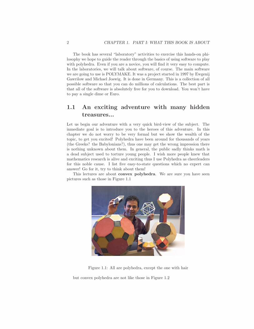
This lectures are about convex polyhedra. We are sure you have seenpictures such as those in Figure 1.1

Figure 1.1: All are polyhedra, except the one with hair

but convex polyhedra are not like those in Figure 1.2

1.1. AN EXCITING ADVENTURE WITH MANY HIDDEN TREASURES...3

Figure 1.2: Polyhedra but not convex!

We will only talk about convex polyhedra in Euclidean space. A convexset S is one for which between any pair of points, the entire line segment iscontained in S.

NOT CONVEX CONVEX

Figure 1.3: Thus a convex set does not look like a croissant!

A hyperplane is given by a linear equation breaks Euclidean space into twopieces called halfspaces (see Figure 1.4). A convex polyhedron is a boundedsubset of Euclidean space that you obtain by intersecting a finite number ofhalf-spaces.

Figure 1.4: A halfspace

What about an infinite number of halfspaces? Can those give polytopes?Well, yes, but in fact the same set would have been easily defined with finitelymany half-spaces, thus why waste so much? On the other hand, all other con-vex figures such as a circle or an ellipse can also be written as intersection ofhalfspaces, but one requires infinitely many of them for sure and thus they are


not polyhedra. One can be very explicit. A polyhedron has a representation asthe set of solutions of a system of linear inequalities.

a1,1x1 + a1,2x2 + · · · + a1,dxd ! b1

a2,1x1 + a2,2x2 + · · · + a2,dxd ! b2

...

ak,1x1 + ak,2x2 + · · · + ak,dxd ! bk

Each inequality represents one halfspace (chosen implicitly by the directionof the inequality). Note that this allows the possibility of using some equationstoo. We will use the standard matrix notation Ax ! b to denote the abovesystem. This is a natural extension of linear algebra. We teach our students howto solve systems of equalities, so why not inequalities? Here’s a little exercisethat will make the transition from linear algebra to polyhedra geometry morenatural: Convince yourself that one can represent a polyhedron as a system oflinear inequalities with only non-negative variables {x : Ax ! b x " 0}. Now,not all polyhedra are bounded (why?), but we focus most of our attention onbounded polyhedra, which will receive the name of polytopes. We will revisitthis with more detail later.

The most evident feature on the “anatomy” of a polytope are its faces. Whatis a face? Essentially, the moment you approach with a hyperplane, at somepoint the plane touches the polyhedron. That’s what you call a face. So, a“corner” is a face. A triangle, of an icosahedron, is a face too. An edge is aface. See Figure 1.5.

From the system of inequalities one can recover the list of all the faces ofdi"erent dimensions. Already this is so simple, but we are going to be askingsome good questions about them!

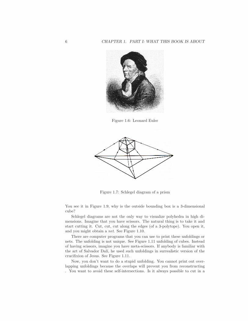
The great swiss mathematician Leonard Euler (Figure 1.6) was one of thefirst to think about the possible numbers of faces of a polytope and the numericrelations between them. Today we know this question is strongly related to otherareas of mathematics such as topology, algebraic geometry and combinatorics.You may have heard of Euler’s surprising equation f0 # f1 + f2 = 2, wheref0 is the number of 0-dimensional faces (or vertices), f1 is the number of 1-dimensional faces (known as edges), and f2 is the number of 2-dimensionalfaces (or facets). You can ask the question, if you give me three numbers, andassign them to the numbers f1, f2, f3, is this triple of numbers coming from apolyhedron? It turns out we know the answer to this question. In 1906, Steinitz(another Swiss mathematician) proved

Theorem 1.1.1 A vector of non-negative integers (f0, f1, f2) is the f -vector ofa 3-dimensional polytope if and only if

1. f0 # f1 + f2 = 2


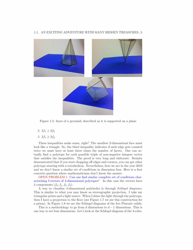
Figure 1.5: faces of a pyramid, described as it is supported on a plane

2. 2f1 " 3f0

3. 2f1 " 3f2

These inequalities make sense, right? The smallest 2-dimensional face mustlook like a triangle. So, the third inequality indicates if each edge gets countedtwice we must have at least three times the number of facets. One can ac-tually find a polytope for each possible triple of non-negative integers vectorthat satisfies the inequalities. The proof is very long and elaborate. Steinitzdemonstrated that if you start chopping o" edges and corners, you can get otherpolytope starting with a tetrahedron. Nevertheless, here we are in the year 2010and we don’t know a similar set of conditions in dimension four. Here is a firstconcrete question where mathematicians don’t know the answer.

OPEN PROBLEM 1: Can one find similar complete set of conditions char-acterizing f-vectors of 4-dimensional polytopes? In this case the vectors have4 components (f0, f1, f2, f3).

A way to visualize 4-dimensional polyhedra is through Schlegel diagrams.This is similar to what you may know as stereographic projection. I take mytriangular prism and a light source. When I shine the light through the polytope,then I have a projection to the floor (see Figure 1.7 we see this construction fora prism). In Figure 1.8 we see the Schlegel diagrams of the five Platonic solids.

This is a methodology to go from d dimensions to d# 1 dimensions. This isone way to see four dimensions. Let’s look at the Schlegel diagram of the 4-cube.


Figure 1.6: Leonard Euler

Figure 1.7: Schlegel diagram of a prism

You see it in Figure 1.9, why is the outside bounding box is a 3-dimensionalcube?

Schlegel diagrams are not the only way to visualize polyhedra in high di-mensions. Imagine that you have scissors. The natural thing is to take it andstart cutting it. Cut, cut, cut along the edges (of a 3-polytope). You open it,and you might obtain a net. See Figure 1.10.

There are computer programs that you can use to print these unfoldings ornets. The unfolding is not unique. See Figure 1.11 unfolding of cubes. Insteadof having scissors, imagine you have meta-scissors. If anybody is familiar withthe art of Salvador Dalı, he used such unfoldings in surrealistic version of thecrucifixion of Jesus. See Figure 1.11.

Now, you don’t want to do a stupid unfolding. You cannot print out over-lapping unfoldings because the overlaps will prevent you from reconstructing. You want to avoid these self-intersections. Is it always possible to cut in a


Figure 1.8: Schlegel diagrams of the Platonic solids

Figure 1.9: Schlegel diagram of a 4-dimensional cube


Figure 1.10: A dodecahedron and two of its unfoldings

Figure 1.11: Net unfoldings of cubes


nice organized way to get a non-self-intersecting unfolding? Well, my friends,nobody knows the answer! This is a simple question for a elementary schoolkid, and we’re all on the same knowledge for the answer.

OPEN PROBLEM 2: Can one always find an unfolding that has no self-overlappings?

One natural question is the number of unfoldings. It is not known if thereis a bound in terms of the f -vector. The exact number of cuts needed is tofind a spanning tree on the (dual) graph. For every spanning tree, you havean unfolding. The question is, is there a spanning tree corresponding to a non-overlapping? I just happened to pick the wrong unfoldings in Figure ??.

Figure 1.12: When unfoldings go wrong and overlap

The questions we discussed so far lie within pure mathematics, but Polyhe-dra are useful in practical calculations. I will touch briefly on some questionsarising from applied mathematics. Linear Programming is a part of Optimiza-tion where you are given a polyhedron (a system of linear inequalities) in R

n

and you want to find a point inside it that maximizes a certain linear functionC = C1x1 + C2x2 + · · · + Cdxd. It turns out that a maximal solution is alwaysfound at a “corner”, a vertex. Solving linear programs is a useful operationperformed thousands of times in various application domains (see []) In mathe-matical terms, you are trying to find the best vertex, the vertex with the bestvalue on this function C. A linear program is written as

maximize C1x1 + C2x2 + · · · + Cdxd

among all x1, x2, . . . , xd, satisfying:


a1,1x1 + a1,2x2 + · · · + a1,dxd ! b1

a2,1x1 + a2,2x2 + · · · + a2,dxd ! b2

...

ak,1x1 + ak,2x2 + · · · + ak,dxd ! bk

George Dantzig invented the simplex algorithm to solve linear programs. Itgoes as follows: We already know the optimal solution is found at a vertex. So,let’s start at a vertex. Then, let’s try to find an adjacent vertex that is better.If that is not already optimal, then move again. Do this again and again. Thenyou reach a vertex where all neighbors are worse. The union of the verticesand edges of a polytope define its graph. The simplex method walks along thegraph of the polytope, each time moving to a better and better cost. followingbeautiful question: How many steps do I need to arrive to an optimal solution?

Figure 1.13: George Dantzig

Performance of the simplex method depends on the diameter of the graph ofthe polytope, i.e., the largest distance between any pair of nodes. The diameteris the largest distance between any pair of nodes. The Hirsch conjecture saysthat the diameter of a polytope is the number of facets1 minus its dimension.This problem remains unsolved after more than 50 years.

1Facets are the faces of highest dimension


OPEN PROBLEM 3: ((the Hirsch conjecture) The diameter of a polytopeP is at most # of facets(P ) # dim(P ).

One of the practical reasons people started to look at polytopes is their vol-ume (or more general integration of functions over polyhedral regions). TheEgyptian pyramid is one of the most famous early polytopes. One of the com-putations we will look at is how to e!ciently compute the volume of polytopes.We pretend that we teach this to calculus students. I’m going convince you thatthere’s much more to it than you can imagine.

For instance, one of the interesting things about computing volumes of poly-hedra is whether using limits is necessary. We tell students to use calculus (andthus use a limit) in integration, but perhaps you can avoid using limits. Here’sone case where we dont limits. Modify the pyramid to have its apex over oneof the base vertices (see Figure ??). If I take three copies of this “distorted”Egyptian pyramid, then I would get a cube. So, three times the volume of thebad Egyptian pyramid is the volume of the cube. That is a special case of theformula we know for all pyramids: one third of the area of the base times theheight.

Figure 1.14: distorted Egyptian pyramid

In dimension two, one can show that no limits are necessary either. If yougive me two polygons of equal area, I can use scissors to cut and rearrange thepieces to transform one into the other. In two dimensions, any two polytopes ofthe same area are equidecomposable (See Figure 1.1). This theorem was provedby Bolyai, the father of Janos Bolyai, co-inventor of non-Euclidean geometries.A finite algorithm exists to find the transformation, and this implies you don’tneed limits to compute areas of polygons because we already know the area of arectangle. The famous 20th century mathematician David Hilbert asked if anytwo convex 3-dimensional polytopes of the same volume are also equidecompos-able. The answer was found less than a year later by Max Dehn.

He proved that there are two 3-polytopes that have the same volume butyet are not equidecomposable! Dehn showed limits are already necessary in the


Figure 1.15: David Hilbert

computation of In some sense, the bad news indicates that you need to studycalculus after all (darn!). Nevertheless, we will look at new ways to computethat won’t look like we need to draw the symbol of integration. It’s a newtechnology that’s not in textbooks yet.

Since we know a formula to compute the volumes of tetrahedra (and pyra-mids) another way to compute volumes is to decompose polytopes into tetrahe-dra and then add the volumes of each piece. But how to decompose or triangu-late a polytope? We will look at ways to triangulate a tetrahedron. Considerthe example of the hexagonal bipyramid show in Figure ??. You can peel itlike an orange, or you can start by decomposing into two pyramids and trian-gulate each. Is there a nice way to find all triangulations of a polyhedron? Fortriangulation here, I am not allowed to add any new vertices.

Another open problem: You give me a 3-dimensional polytope. If you giveme triangulations of two di"erent sizes, is there a triangulation of every inter-


6 8

Figure 1.16: many ways to triangulate a bipyramid

mediate size? We don’t know!OPEN PROBLEM 4: If for a 3-dimensional polyhedron P we know that thereis triangulation of size k1 and triangulations of size k2, with k2 > k1 is there atriangulation of every size k, with k1 < k < k2?

Another practical problem is to count the number of lattice points insidea polyhedron. A wide variety of topics in pure and applied mathematics in-volve the practical problem of counting the number of lattice points inside a apolytope. Applications range from the very pure (number theory, commutativealgebra, representation theory) to the most applied (cryptography, computer sci-ence, optimization, and statistics). For example, An emerging new application oflattice point counting is computer program verification and code optimization.The systematic reasoning about a program’s runtime behavior, performance,and exe cution requires specific knowledge of the number of operations and re-source allocation within the program. This is importan t knowledge for the sakeof checking correctness as well as for automatically detecting run-time errors,bu"er overflows, null-pointer dereferen ces or memory leaks. For example, howoften is instruction I of the following computer code executed?

void proc(int N, int M){int i,j;for (i=2N-M; i<= 4N+M-min(N,M), i++)for(j=0; j<N-2*i; j++)I;

}

Clearly, the number of times we reach instruction I depends parametricallyon N,M. In terms of these parameters the set of all possible solutions is given bythe number of lattice points inside of a parametrized family of polygons. In our


toy example these are described by the conditions {(i, j) $ Z2 : i " 2N#M, i !4N + M # min(N, M), j " 0, j # 2i ! N # 1}.

When you count lattice points, you can approximate the volume. If youdilate a polytope to be larger, it’s essentially the same as making a smallerlattice. It’s the same as adding tiny little cubes around the lattice points. So,it’s like a Riemann Integration. Integration is another reason to look at countinglattice points.

Many objects can be counted as the lattice points in some polytope: Exam-ples include, Sudoku configurations, routes on a network, and magic squares.These are n%n squares whose entries are non-negative integers with sums overrows columns and diagonals equal to a constant, the magic number (see Figure1.17. Mathematically, the possible magic squares are non-negative integer solu-tions of a system of equations and inequalities: 2n + 2 equations, one for eachrow sum, column sum, and diagonal sum. For example for 4%4 magic squares ofmagic sum 24 we have x11+x12+x13+x14 = 24, first rowx13+x23+x33+x43 =24, third column, and of course xij " 0

5

12 0 5 7

0 12 7 5

7 5 0 12

5 7 12 0

Figure 1.17: 4 % 4 magic squares with magic sum 24

One beautiful puzzle is to determine the number of magic squares of a givensize. This problem is really asking about the number of lattice points in aparticular polytope. We can ask

OPEN PROBLEM 5: Find a formula in terms of k for the number of 30%30magic squares with magic sum k.

It is already non-trivial to figure out one concrete value, say k = 10. Thisis a challenge of computation which is well beyond humanity’s reach today.

1.2 The Rest of this Book

• Basic polyhedral geometry. (week 2) Representation of polyhedra, dimen-sion.

1.2. THE REST OF THIS BOOK 15

• Rules of computation and measuring e!ciency introduction to POLY-MAKE. (week 1)

• Computer representation of polytopes: facets vs. vertices, chirotopes.(week 3-4)

• Visualization of Polytopes: Schlegel Diagrams, Nets, Gale Transforms,Slices and Projections. (week 5)

——————–

• Polytope graphs (project).

• Finding decompositions and triangulations. (project)

• Volumes, integrals, and discrete Sums over polytopes. (project)

• Containment, Distance, Width, and Approximation problems. (project)

• Symmetry of polytopes and polyhedra. (project)

Chapter 2

PART II: Basics of

Polyhedral Geometry

We will get more technical during this session (Let’s make very precise themeanings of our words). We assume the reader is comfortable with linear algebraand the basics of analysis. We also assume the reader has studied the firstthirteen sections of the lecture notes Theory of Convex Sets by G.D. Chakerianand J.R. Sangwine-Yager

2.1 Polyhedral Notions

Everything we do takes place inside Euclidean d-dimensional space Rd. We

have the traditional Euclidean distance between two points x, y defined by!

(x1 # y1)2 + . . . (x2 # y2)2. Given two points x, y. We will use the common

fact that Rd

is a real vector space and thus we know how to add or scale itspoints.

Definition 2.1.1 A subset S of Rn is called convex if for any two distinctpoints x1, x2 in S the line segment joining x1, x2, lies completely in S. This isequivalent to saying x = !x1 +(1#!)x2 belongs to S for all choices of ! between0 and 1.

In general, given a finite set of points A = {x1, . . . , xn}, we say that a linearcombination

"

"ixi is

• an a!ne combination if"

"i = 1

• a convex combination if it is a!ne and "i " 0 for all i.

17

18 CHAPTER 2. PART II: BASICS OF POLYHEDRAL GEOMETRY

We will assume that the empty set is also convex. Observe that the intersec-

tion of convex sets is convex too. Let A & Rd, the convex hull of A, denoted by

conv(A), is the intersection of all the convex sets containing A. In other words,A is the smallest convex set containing A. The reader can check that the imageof a convex set under a linear transformation is again a convex set.

Recall from linear algebra that a linear function f : Rd' R is given by a

vector c $ Rd, c (= 0. For a number # $ R we say that H! = {x $ R

d: f(x) =

#} is an a!ne hyperplane or hyperplane for short. Note that a hyperplane

divides Rd

into two halfspaces H+! = {x $ R

d: f(x) " #} and H!

! = {x $ Rd

:f(x) ! #}. Halfspaces are convex sets.

We begin with the key definition of this notes:

Definition 2.1.2 The set of solutions of a system of linear inequalities is calleda polyhedron. In its general form a polyhedron is then a set of the type

P = {x $ Rd

:< ci, x >! $i}

for some non-zero vectors ci in Rd

and some real numbers $i.

In other words A polyhedron in Rd

is the intersection of finitely many halfspaces.By the way, the plural of the word polyhedron is polyhedra.

Lemma 2.1.1 Let Ax ! b, Cx " d, be a system of inequalities. The set ofsolutions is a convex set.

Write a proof!Although everybody has seen pictures or models of two and three dimen-

sional polyhedra such as cubes and triangles and most people may have a mentalpicture of what edges, ridges, or facets for these objects are, we will formallyintroduce them later on. Now another important definition:

Definition 2.1.3 A polytope is the convex hull of a finite set of points in Rd.

Lemma 2.1.2 For a set A & Rd

we have that conv(A) equals the set of all

possible convex combinations. In particular, for a finite set of points in Rd

A := {a1, a2, . . . , an} we have that conv(A) equals

2.1. POLYHEDRAL NOTIONS 19

{n

#

i=1

"iai : "i " 0 and "1 + . . . "n = 1}

Exercise: Write a proof!Related to minimal size representations of a vector as a convex combinations

we have

Theorem 2.1.3 (Caratheodory’s Theorem) If x $ conv(S) in Rd, then xis the convex combination of d + 1 points in S.

Write a proofYou can actually find d + 1 points that actually su!ce to write a point in

the set. If you have, for instance

x $N

#

i=1

"iyi

for some huge number N , the theorem here guarantees that you can do this usinga sum of not so many summands. This is not necessarily about polytopes. Thisis a true fact about convexity in general. In polytopes, you have the advantagethat you know the set S is already finite to start with. As a corollary, all trianglesof a polygon (using the vertices of the polygon) must cover the polygon.

Now it is easier to speak about examples of polytopes. We invite you to findmore on your own! Here are some basic examples.

1. Standard Simplex Let e1, e2, . . . , ed+1 be the standard unit vectors in

Rd+1

. The standard d-dimensional simplex #d is conv({e1, . . . , ed+1}).From the above lemma we see that the set is precisely

#d = {x = (x1, . . . , xd+1) : xi " 0 and x1 + x2 + · · · + xd+1 = 1}.

Note that for a polytope P = conv({a1, . . . , am}) we can define a linearmap f : #m!1 ' P by the formula f(!1, . . . ,!m) = !1a1 + · · · + !mam.Lemma 2.1.2 implies that f(#m!1) = P . Hence, every polytope is theimage of the standard simplex under a linear transformation. A lot of theproperties of the standard simplex are then shared by all polytopes.

2. Standard Cube Let {ui : i $ I} be the set of all 2d vectors in Rd

whosecoordinates are either 1 or -1. The polytope Id = conv({ui : i $ I} iscalled the standard d-dimensional cube. The images of a cube underlinear transformations receive the name of zonotopes.

Clearly Id = {x = (x1, . . . , xd) : #1 ! xi ! 1}


3. Standard Crosspolytope This is the convex hull of the 2d vectorse1,#e1, e2,#e2, . . . , ed,#ed. The 3-dimensional crosspolytope is simplyan octahedron.

4. A d-pyramid is the convex hull of a (d # 1)-polytope Q and a point notin the a!ne hull of Q.

5. A d-prism is the convex hull of two (d# 1)-polytopes P, P " where P " is atranslate of P that does not lie in the a!ne hull of P .

6. A d-bipyramid is the convex hul of a (d # 1)-polytope and a segmentthat intersects the interior of P , with one point on one side of the a!nehull of P and the other end point on the other side.

Let P be a polytope in Rd. A linear inequality f(x) ! # is said to be valid

on P if every point in P satisfies it. A set F & P is a face of P if and onlythere exists a linear inequality f(x) ! # which is valid on P and such thatF = {x $ P : f(x) = #}. In this case f is called a supporting function of F andthe hyperplane defined by f is a supporting hyperplane of F .

For a face F consider the smallest a!ne subspace aff(F ) in Rd

generated byF . Its dimension is called the dimension of F . Similarly we define the dimensionof the polytope P . We like to think of the polytope and the empty set as faces.They are honorary faces of the polytope!

Another, equivalent definition of dimension is in terms of a!ne indepen-dence. This generalizes the notion of linear independence. We say that a set ofpoints is a!nely dependent if there is a linear combination of the xi equal to0, where

"

"i = 0 but not all "i are zero. One can prove that A set of d + 2points in Rd is always a!nely dependent. A set of points that is not a!nelydependent is a!nely independent. The dimension of subset X of R

ncan be

defined as the size of any maximal a!nely independent set of points in X .

Definition 2.1.4 A point x is a convex set S is an extreme point of S if it isnot an interior point of any line segment in S. This is equivalent to saying thatwhen x = !x1 + (1 # !)x2, then either ! = 1 or ! = 0.

Lemma 2.1.4 Every vertex of a polyhedron is an extreme point.

Exercise: Write a proof!!

2.2 The characteristic features of Polyhedra

We want to be able to compute the essential features of a polyhedron or a poly-tope. Among them we wish to find out what are their faces or extreme points,we wish to know what is their dimension, whether the polyhedron in question isempty or not. We want to answer such questions with concrete practical algo-rithms. So far we have consider polyhedra as given by a system of inequalitiesof the form Ax ! b. Now we disclose other equivalent representations:

2.2. THE CHARACTERISTIC FEATURES OF POLYHEDRA 21

2.2.1 Equivalent representations of polyhedra, dimensionand extreme points

Lemma 2.2.1 Given a bounded polyhedron P = {x $ Rn | Ax ! b} then

• There is a translation of P that can be represented with in the form {x $Rn : A"x ! b" and x " 0}.

• There is a polyhedron of the form Q = {x $ Rq : Bx = c, x " 0} such that

– the coordinate-erasing linear projection

% : Rq #' Rn : x = (x1, . . . , xn, . . . xq) )' %(x) = (x1, . . . , xn)

provides a bijection between Q and P .

– The bijection implies that %(Q * Zq) = P * Zn.

– y $ Q is an extreme point if and only if %(x) is an extreme point ofP

– dim(Q) = dim(P ).

Write a proof

Lemma 2.2.2 The set of all n % n matrices whose sums along rows, columns,or diagonals are equal to the same constant (magic squares) k is a boundedpolyhedron

Exercise: Write a proofWe will state a lemma that will allow us to compute the dimension from a

polyhedron. From Theorem ?? it is enough to explain it for polyhedra givenin the form {x : Ax = b}. A face of dimension 0 is called a vertex. A face ofdimension 1 is called an edge, and a face of dimension dim(P ) # 1 is called afacet. The empty set is defined to be a face of P of dimension #1. Faces thatare not the empty set or P itself are called proper. Let us look at a simplerecipe for the dimension.

Lemma 2.2.3 Given P = {x $ Rn | Ax = b x " 0}, the dimension of P isn # rank(A).

Write a proofGiven the example we have for the 4% 4 magic squares, the matrix A is

$

%

%

%

%

%

%

%

%

%

%

&

1 1 1 11 1 1 1

1 1 1 11 1 1 1

1 1 1 11 1 1 1

1 1 1 11 1 1 1

'

(

(

(

(

(

(

(

(

(

(

)

(2.1)


This matrix is not full rank. The rank of A is 7. There are sixteen variables.So, by the lemma above, the dimension is 16# 7. The formula has been verifiedin this example.

Lemma 2.2.4 The dimension of the polyhedron Mn#n(k) of all n % n magicsquares with magic sum is equal to (n # 1)2.

Write a proof

Theorem 2.2.1 Consider the polyhedron given by Ax = b, x " 0. Suppose them columns Ai1 , Ai2 , . . . , Aim

of the m % n matrix A are linearly independentand there exist non-negative numbers xij

such that

xi1Ai1 + xi2Ai2 + · · · + ximAim

= b.

Then the points with entry xijin position ij and zero elsewhere is an extreme

point of the polyhedron P = {x : Ax = b, x " 0}.

Proof: Suppose x is not a extreme point. Then x lies in the interior of a linesegment in P = {y : Ay = b, y " 0}. Thus x = !u + (1 # !)v with ! between 0and 1. But this implies, by looking at the entries of x that are zero, that u, valso have that property. Now, consider y = x # u. A(x # u) = 0 but since thecolumns Ai1 , Ai2 , . . . , Aim

are linearly independent, x = u, a contradiction.

Theorem 2.2.2 Suppose x = (x1, . . . , xn) is an extreme point of a polyhedronP = {x : Ax = b, x " 0} with A an m % n matrix. Then

1) the columns of A which correspond to positive entries of x form a linearlyindependent set of vectors in Rm

2) At most m of the entries of x can be positive, the rest are zero.

Proof: Suppose the columns are linearly dependent. Thus there are coe!cients,not all zero, such that ci1Ai1 + ci2Ai2 + · · · + cim

Aim= 0

Thus we can form points(xi1 # dci1)Ai1 + (xi2 # dci2)Ai2 + · · · + (xim

# dcim)Aim

= b(xi1 + dci1)Ai1 + (xi2 + dci2)Ai2 + · · · + (xim

+ dcim)Aim

= bSince d is any scalar, we may choose d less than the minimum of xj/|cj | for

those cj (= 0.We have reached a contradiction! Since x = 1/2(u) + 1/2(v) and both u, v

are inside the polyhedron. For part (2) simply observe that there cannot bemore than m linearly independent vectors inside Rm.

Exercise 2.2.5 Find all the extreme points of the polyhedron M3#3(1).

Write a solution!

Definition 2.2.3 A basic solution is a a solution of the system Ax = b wheren # m variables are set to zero. If in addition the solutions happens to havex " 0 then we say is basic feasible solution.

In any basic solution, the n # m variables which are set equal to zero arecalled nonbasic variables and the m variables we solved for are called the basicvariables.

2.3. WEYL-MINKOWSKI AND POLARITY 23

We can rephrase the above results by saying that the extreme points of thepolyhedron P = {x : Ax = b, x " 0} are precisely the basic feasible solutions.By Krein-Milman’s theorem we know now that if P is bounded then it is theconvex hull of its basic feasible points.

Lemma 2.2.6 Every basic feasible of a polyhedron {x : Ax = b, x " 0} is avertex.

Corollary 2.2.7 For a polyhedron of the form P = {x : Ax = b, x " 0}, thesets of basic feasible solutions, vertices, and extreme points are identical.

Write a proof!

2.3 Weyl-Minkowski and Polarity

It makes sense to study the relation between polytopes and polyhedra. Clearlystandard cubes,simplices and crosspolytopes are also polyhedra, but is this thecase in general? What one expects is really true. Polytopes are special kind ofpolyhedra, but not all polyhedra are polytopes.

Theorem 2.3.1 (Weyl-Minkowski theorem) Every polytope is a polyhedron.Every bounded polyhedron is a polytope.

Figure 2.1: H. Weyl and H. Minkowski

This theorem is very important. Having this double way of representinga polytope allows you to work, using either the vertex representation or theinequality representation representation, what would be hard to prove usinga single representation becomes easy with the other. For example, every in-tersection of a polytope with an a!ne subspace is a polytope. Similarly, theintersection of finitely many polytopes is a polytope. Both statements are rathereasy to prove if one knows that polytopes are just given by systems of linear


inequalities, since then the intersection of polytopes is just adding new equa-tions. On the other hand, It is known that every linear projection of a boundedpolyhedron is a bounded polyhedron. To prove this from the inequality rep-resentation is di!cult, but it is easy when one observes that the projection ofconvex hull is the convex hull of the projection of the vertices of the polytope.In addition, the Weyl-Minkowski theorem is very useful in applications! its ex-istence is key in the field of combinatorial and linear optimization. We can givea non-constructive proof here and later an algorithmic proof.

Definition 2.3.1 A representation of a polytope by a set of inequalities, is anH-representation. On the other hand, when a polytope is given a convex hull ofa set of points we have a V-representation.

Before we discuss a proof of Weyl-Minkowski theorem we need to introducea useful operation. To every subset of Euclidean space we wish to associate a

convex set. Given a subset A of Rd

the polar of A is the set Ao in Rd

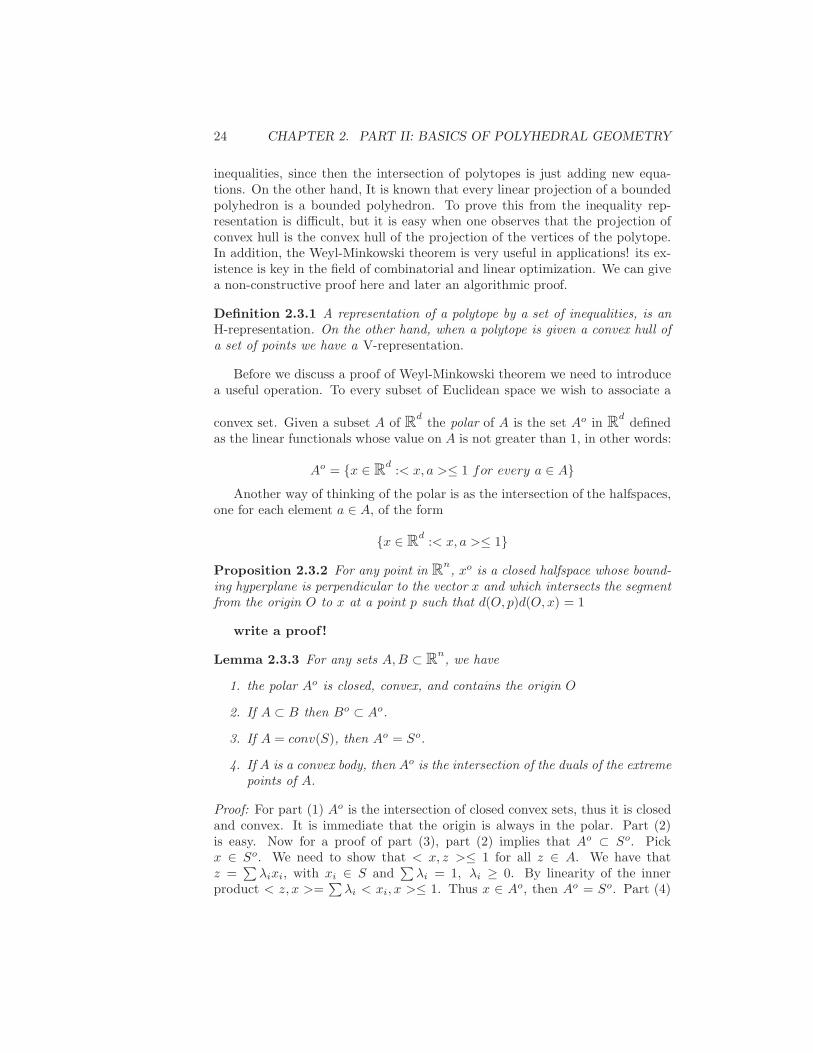
definedas the linear functionals whose value on A is not greater than 1, in other words:

Ao = {x $ Rd

:< x, a >! 1 for every a $ A}

Another way of thinking of the polar is as the intersection of the halfspaces,one for each element a $ A, of the form

{x $ Rd

:< x, a >! 1}

Proposition 2.3.2 For any point in Rn, xo is a closed halfspace whose bound-

ing hyperplane is perpendicular to the vector x and which intersects the segmentfrom the origin O to x at a point p such that d(O, p)d(O, x) = 1

write a proof!

Lemma 2.3.3 For any sets A, B & Rn, we have

1. the polar Ao is closed, convex, and contains the origin O

2. If A & B then Bo & Ao.

3. If A = conv(S), then Ao = So.

4. If A is a convex body, then Ao is the intersection of the duals of the extremepoints of A.

Proof: For part (1) Ao is the intersection of closed convex sets, thus it is closedand convex. It is immediate that the origin is always in the polar. Part (2)is easy. Now for a proof of part (3), part (2) implies that Ao & So. Pickx $ So. We need to show that < x, z >! 1 for all z $ A. We have thatz =

"

!ixi, with xi $ S and"

!i = 1, !i " 0. By linearity of the innerproduct < z, x >=

"

!i < xi, x >! 1. Thus x $ Ao, then Ao = So. Part (4)

2.3. WEYL-MINKOWSKI AND POLARITY 25

is direct from part (3) because Krein-Milman says a convex body is the convexhull of its extreme points.

Here are two more useful examples of polarity: Take L a line in R2

passingthrough the origin, what is L0? Well the answer is the perpendicular line thatpasses through the origin. If the line does not pass through the origin the answeris di"erent. What is it? Answer: it is a clipped line orthogonal to the given linethat passes through the origin. To see without loss of generality rotate the lineuntil it is of the form x = c (because the calculation of the polar boils down tochecking angles and lengths between vectors we must get the same answer upto rotation).

What happens with a circle of radius one with center at the origin? Its polarset is the disk of radius one with center at the origin. Next take B(0, r). Whatis B(0, r)o? The concept of polar is rather useful. We use the following lemma:

Lemma 2.3.4 1. If P is a polytope and 0 $ P , then (P o)o = P .

2. Let P & Rd

be a polytope. Then P o is a polyhedron.

Write a proof!Now, using the above lemma, we are ready to prove the Weyl-Minkowski

theorem:Proof: ( of Weyl-Minkowski) First we verify that a bounded polyhedron is a

polytope: Let P be {x $ Rd

:< x, ci >! bi}.Consider the set of points E in P that are the unique intersection of d or

more of the defining hyperplanes. The cardinality of E is at most*m

d

+

so it isclearly a finite set and all its element are on the boundary of P . Denote byQ the convex hull of all elements of E. Clearly Q is a polytope and Q & P .We claim that Q = P . Suppose there is a y $ P # Q. Since Q is closed andbounded (bounded) we can find a linear functional f with the property thatf(y) > f(x) for all x $ Q. Now P is compact too, hence f attains its maximumon the boundary moreover we claim it must reach it in a point of E. The reasonis that a boundary point that is not in E is in the solution set

We verify next that a polytope is indeed a polyhedron: We can assumethat the polytope contains the origin in its interior (otherwise translate). Sofor a su!ciently small ball centered at the origin we have B(0, r) & P . HenceP o & B(0, r)o = B(0, 1/r). This implies that P o is a bounded polyhedron. Butwe saw in the first part that bounded polyhedra are polytopes. Then P o is apolytope. We are done because we know from the above lemma that (P o)o = Pand polar of polytopes are polyhedra.

From this fundamental theorem several nice consequences follow:

Corollary 2.3.5 Let P be a d-dimensional polytope in Rd. Then


1. The intersection of P with a hyperplane is a polytope. If the hyperplanepasses through a point in the relative interior of P then the intersection isa (d # 1)-polytope.

2. Every projection of P is a polytope. More generally, the image of P undera linear map is another polytope.

Write a proof!Proof: Part (1) follows because a polytope is a bounded polyhedron but theintersection of a polyhedron with a hyperplane gives a polyhedron of lower di-mension which is still bounded, thus the result is a polytope. The points of P areconvex combinations of vertices v1, . . . , vm then applying a linear transforma-tion %, we see linearity implies that any point of %(P ) is a convex combinationof %(v1), . . . ,%(vm).

Chapter 3

PART III: Fourier-Motzkin

Elimination and its

Applications

3.1 Feasibility of Polyhedra and Facet-Vertex rep-

resentability

In this section we take care of various important issues. Our very first algorithmwill be about deciding when a polyhedron (system of inequalities) is empty ornot. We are also interested in practical ways of going from H-representationto V-representation or vice versa. Our new proof of Weyl-Minkowski was non-constructive.

3.1.1 Solving Systems of Linear Inequalities in Practice

When is a polytope empty? Can this be decided algorithmically? How can onesolve a system of linear inequalities Ax ! b? We start this topic looking backon the already familiar problem of how to solve systems of linear equations. Itis a crucial algorithmic step in many areas of mathematics and also would helpus better understand the new problem of solving systems of linear inequalities.Recall the fundamental problem of linear algebra isProblem: Given an m % n matrix A with rational coe!cients, and a rationalvector b $ Qm, is there a solution of Ax = b? If there is solution we want tofind one, else, can one produce a proof that no solution exist?

I am sure you are well-aware of the Gaussian elimination algorithm to solvesuch systems. Thanks to this and other algorithms we can answer the firstquestion. Something that is usually not stressed in linear algebra courses is thatwhen the system is infeasible (this is a fancy word to mean no solution exists)Gaussian elimination can provide a proof that the system is indeed infeasible!

27

28CHAPTER 3. PART III: FOURIER-MOTZKIN ELIMINATION AND ITS APPLICATIONS

This is summarized in the following theorem:

Theorem 3.1.1 (Fredholm’s theorem of the Alternative) The system oflinear equations Ax=b has a solution if and only for each y with the propertythat yA = 0, then yb = 0 as well.

In other words, one and only one of the following things can occur: EitherAx = b has solution or there exist a vector y with the property that yA = 0 butyb (= 0. Similarly {x | Ax = b} is non-empty if and only if {y | yT A = 0, yT b =#1} is empty.

So think of this as a mathematical proof that some system has no solution!The vector y above is a mathematical proof that Ax = b has no solution. Tosolve Ax = b? We teach them Gaussian elimination. We teach row operationsthat put the matrix in a certain reduced form. We know then that the entriesof b change. What we teach undergraduates is there is no solution when thereis a row zeroes in the reduced A but a non-zero entry in the corresponding b. Ifthe string of matrices

Mk · · ·M2M1

are the elementary matrices that reduce A, then

y = edMk · · ·M2M1

This shows that yT A = 0 and yT b = #1.

Thus when Ax = b has no solution we get a certificate, a proof that thesystem is infeasible. But, how does one compute this special certificate vectory? With care, it can be carefully extracted from the Gaussian elimination. Hereis how: The system Ax = b can be written as an extended matrix.

$

%

%

%

%

%

%

&

a11 a12 . . . a1n b1

a21 a22 . . . a2n b2

......

......

...

am1 am2 . . . amn bm

'

(

(

(

(

(

(

)

We perform row operations to eliminate the first variable from the second,third rows. Say a11 is non-zero (otherwise reorder the equations). Substractmultiples of the first row from the second row, third row, etc. Note that this isthe same as multiplying the extended matrix, on the left, by elementary lowertriangular matrices. After no more than m steps the new extended matrix lookslike.

3.1. FEASIBILITY OF POLYHEDRA AND FACET-VERTEX REPRESENTABILITY29

$

%

%

%

%

%

%

&

a11 a12 . . . a1n b1

0 a"22 . . . a"

2n b"2

......

......

...

0 a"m2 . . . a"

mn b"m

'

(

(

(

(

(

(

)

Now the last m# 1 rows have one less column. Recursively solve the systemof m # 1 equations. What happens is the variables have to be eliminated in allbut one of the equations creating eventually a row-echelon shaped matrix B.Again all these row operations are the same as multiplying A on the left by acertain matrix U . If there is a solution of this smaller system, then to obtainthe solution value for the variable x1 can be done by substituing the values inthe first equation. When there is no solution we detect this because one of therows, say the i-th row, in the row-echelon shaped matrix B has zeros until thelast column where it is non-zero. The certificate vector y is given then by thei-th row of the matrix U which is the one producing a contradition 0 = c (= 0.

If you are familiar with the concerns of numerical analysis, you may beconcerned about believing the vector y is an exact proof of infeasibility. “Whatif there are round of errors? Can one trust the existence of y?” you will say.Well, you are right! It is good time to stress a fundamental di"erence in thislecture from what you learned in a numerical analysis course: Operations areperformed using exact arithmetic not floating point arithmetic. We can trustthe identities discovered as exact.

Unfortunately, in many situations finding just any solution might not beenough. Consider the following situations:

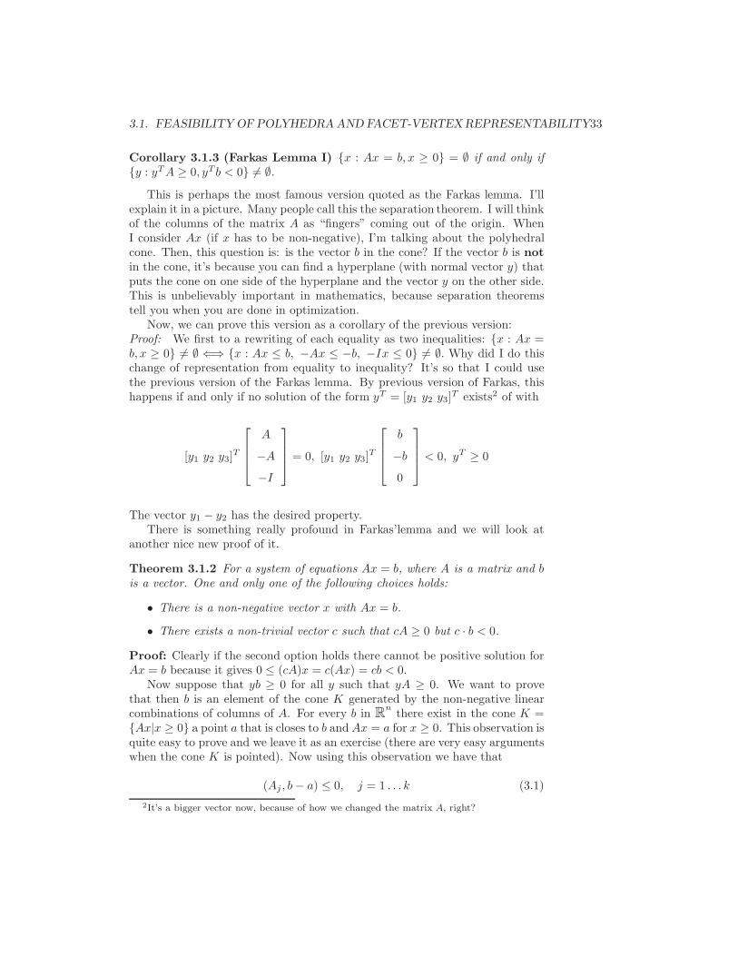
Suppose a friend of yours claims to have a 3% 3 % 3 array of numbers, withthe property that when adding 3 of the numbers along vertical lines or anyhorizontal row or column you get the numbers shown in Figure 3.1:

The challenge is to figure out whether your friend is telling the truth or not?Clearly because the numbers in the figure are in fact integer numbers one canhope for an integral solution, or even for a nonnegative integral solution becausethe numbers are non-negative integers. This suggests three interesting variationsof linear algebra. We present them more or less in order of di!culty here below.We begin now studying an algorithm to solve problem A. We will encounterproblems B and C later on. Can you guess which of the three problems isharder in practice?Problem A: Given a rational matrix A $ Qm#n and a rational vector b $ Qm.Is there a solution for the system Ax = b, x " 0, i.e. a solution with allnon-negative entries? If yes, find one, otherwise give a proof of infeasibility.Problem B: Given an integral matrix A $ Zm#n and an integral vector b $ Zm.Is there a solution for the system Ax = b, with x an integral vector? If yes, finda solution, otherwise, find a proof of infeasibility.


5 22

2

2

2

22

2

2

22

3

3

33

3

1

1

1

1

1

1

3

3

5

4

Figure 3.1: A cubical array of 27 seven numbers and the 27 line sums

Problem C: Given an integral matrix A $ Zm#n and an integral vector b $ Zm.Is there a solution for the system Ax = b, x " 0? i.e. a solution x using onlynon-negative integer numbers? If yes, find a solution, otherwise, find a proof ofinfeasibility.

I want this similar result for polyhedra. It’s called Farkas lemma:

Theorem 3.1.1 (Farkas Lemma) A polyhedron {x | Ax ! b} is non-emptyif and only if there is no solution to {y | yT A = 0, yT b < 0, y " 0}.

To prove this theorem, I’m actually going to give you an algorithmic proof.If the polyhedron is non-empty, it will give you an explicit solution. Otherwise,it will tell you how to develop a certificate y. The algorithm is an ine!cient(non-polynomial time algorithm) algorithm to decide this. The algorithm iscalled the Fourier-Motzkin algorithm. It was reinvented by Motzkin. Fourierdiscovered this centuries ago, and it was completely forgotten. Moreover, laterwe will derive the transformation from H-representation to V-representation andback.

3.1.2 Fourier-Motzkin Elimination and Farkas Lemma

The input of this algorithm is a polyhedron {x | Ax ! b}. The output is a yesor a no.

Let’s deal with the case of just one variable. For example,


Example 3.1.2

7x1 ! 3

3x1 ! 2

2x1 ! 0

#4x1 ! 4

We know this one is possible, because we write this as

x1 !3

7

x1 !2

3

x1 ! 0

x1 " #1

If P is described by a single variable x, P is feasible if

max(bi/ai | bi/ai < 0 ! min(bj/aj | bj/aj > 0.

So, we know what to do in one variable. We should do an induction. Ifthere is more than one variable, then we eliminate the leading variable x1. Werewrite the inequalities to be regrouped into three kinds:

x1 + (a"i)

T x" ! b"i, (if coe!cient of ai1 is positive) (TYPE I)

#x1 + (a"j)

T x" ! b"j , (if coe!cient of aj1 is negative) (TYPE II)

(a"k)T x" ! b"k, (if coe!cient of ak1 is zero) (TYPE III)

Here x" = (x2, x3, . . . , xn).For the type IIs, these are obtained by dividing by |aj1| on both sides. Here

comes the hocus pocus. The +1 and #1 coe!cients on x1 on the types I andtypes II cancel out. Now, the computational trouble is that if you have 1 millionof type I and 1 million of type II, there’s 1 million squared of these. We justkeep the equations of type III. Original system of inequalities has a solution ifand only if the system (+) is feasible

(+) is equivalent to (a"j)

T x # bj ! bi # (a"i)

T x", and (a"k)T x" ! b"k

If we find x2, x3, . . . , xn satisfying (+), find

max((a"j)

T x # bj) ! x1 ! min(bi # (a"i)

T x").


The process ends when we have a single variable.An equation of the first type

x1 + (a"i)

T x" ! b"i

is nowx1 ! b"i # (a"

i)T x"

and the second type#x1 + (a"

j)T x" ! b"j

is now#x1 " (a"

j)T x" # b"j

Then we can look at the solution for x1.This is essentially the algorithm. It’s a beautiful method, but I wouldn’t

suggest it for my family to do. There is a polynomial time method, called theellipsoid method. But it’s not a strongly polynomial time method. Now, Iwouldn’t recommend my family to do this method either! It is a polynomialtime feasibility/decision problem. However, it’s not really practical quite yet.The state of the art is really the simplex method. It can be used (and is usedby engineers) to see if a polyhedron is empty or not.

Now, is the simplex method polynomial time? Actually the method dependson your choice of pivot, given by a pivot rule. There are actually, then, manysimplex methods! My academic grandfather Victor Klee1 crafted an examplewith Minty that takes an exponential number of pivots. In some sense, here’s theirony of life: in practice, people use the simplex method, though theoreticallyexponential.

So, let’s try to prove the Farkas lemma. We kill one variable at each iterationuntil we are in a single variable system. The new system will have no variables:

$

%

%

%

&

00...0

'

(

(

(

)

!

$

%

%

%

&

b"1b"2...

b"n

'

(

(

(

)

The polyhedron {x | Ax ! b} is infeasible if and only if b"i < 0 for some i.So the rewriting and addition steps correspond to row operations on the

original matrix A.r = MAx " Mb = b"

with matrix M with non-negative entries. We set yT = (ei)T M , with ei standardi-th unit vector then

0 = yT A, yT b < 0, and y " 0.

Here is another form of Farkas lemma:1A great supporter of the MAA, he passed away recently


Corollary 3.1.3 (Farkas Lemma I) {x : Ax = b, x " 0} = , if and only if{y : yT A " 0, yT b < 0} (= ,.

This is perhaps the most famous version quoted as the Farkas lemma. I’llexplain it in a picture. Many people call this the separation theorem. I will thinkof the columns of the matrix A as “fingers” coming out of the origin. WhenI consider Ax (if x has to be non-negative), I’m talking about the polyhedralcone. Then, this question is: is the vector b in the cone? If the vector b is notin the cone, it’s because you can find a hyperplane (with normal vector y) thatputs the cone on one side of the hyperplane and the vector y on the other side.This is unbelievably important in mathematics, because separation theoremstell you when you are done in optimization.

Now, we can prove this version as a corollary of the previous version:Proof: We first to a rewriting of each equality as two inequalities: {x : Ax =b, x " 0} (= , -. {x : Ax ! b, #Ax ! #b, #Ix ! 0} (= ,. Why did I do thischange of representation from equality to inequality? It’s so that I could usethe previous version of the Farkas lemma. By previous version of Farkas, thishappens if and only if no solution of the form yT = [y1 y2 y3]T exists2 of with

[y1 y2 y3]T

$

%

%

&

A

#A

#I

'

(

(

)

= 0, [y1 y2 y3]T

$

%

%

&

b

#b

0

'

(

(

)

< 0, yT " 0

The vector y1 # y2 has the desired property.There is something really profound in Farkas’lemma and we will look at

another nice new proof of it.

Theorem 3.1.2 For a system of equations Ax = b, where A is a matrix and bis a vector. One and only one of the following choices holds:

• There is a non-negative vector x with Ax = b.

• There exists a non-trivial vector c such that cA " 0 but c · b < 0.

Proof: Clearly if the second option holds there cannot be positive solution forAx = b because it gives 0 ! (cA)x = c(Ax) = cb < 0.

Now suppose that yb " 0 for all y such that yA " 0. We want to provethat then b is an element of the cone K generated by the non-negative linearcombinations of columns of A. For every b in R

nthere exist in the cone K =

{Ax|x " 0} a point a that is closes to b and Ax = a for x " 0. This observation isquite easy to prove and we leave it as an exercise (there are very easy argumentswhen the cone K is pointed). Now using this observation we have that

(Aj , b # a) ! 0, j = 1 . . . k (3.1)

2It’s a bigger vector now, because of how we changed the matrix A, right?


and

(#a, b # a) ! 0. (3.2)

Why? the reason is a simple inequality on dot products. If we do not havethe inequalities above we get for su!ciently small t $ (0, 1):

|b # (a + tAj)|2 = |(b # a) # tAj |

2 =

|b # a|2 # 2t(Aj , b # a) + t2|Aj |2 < |b # a|2

or similarly we would get

|b # (a # ta)|2 = |(b # a) + ta|2 = |b # a|2 # 2t(#a, b # a) + t2|a|2| < |b # a|2

Both inequalities contradict the choice of b because a + tAj is in K andthe same is true for a # ta = (1 # t)a $ K. We have then that from thehypothesis and the equations in (ONE) that (b,#(b#a)) " 0, which is the sameas (b, b # a) ! 0 and this together with equation (TWO) (#a, b # a) ! 0 gives(b # a, b # a) = 0, and in consequence b = a. !

The theorem above is equivalent to

Theorem 3.1.3 For a system of inequalities Ax ! b, where A is a matrix andb is a vector. One and only one of the following choices holds:

• There is a vector x with Ax ! b.

• There exists a vector c such that c · b < 0, c " 0,"

ci > 0, and cA = 0.

The reason is simple, The system of inequalities Ax ! b has a solution ifand only if for the matrix A" = [I, A,#A] there is a non-negative solution toA"x = b. The rest is only a translation of the previous theorem in the secondalternative. If you tried to solve the strict inequalities in the system Bx < 0,like the one we got for deciding convexity of pictures, you would run into troublesfor most computer programs (e.g. MAPLE, MATHEMATICA,etc). One needsto observe that a system of strict inequalities Bx < 0 has a solution preciselywhen Bx ! #1 has a solution. If the solution x gives Bx < #1/q for instancepx is a solution for the strict inequality and vice versa. Thus the above theoremimplies the Farkas’ lemma version we saw earlier.

There are millions of version of Farkas lemmas. Here is another one:

Corollary 3.1.4 (Farkas Lemma II) {x : Ax ! b, x " 0} (= , -. When yT A "0, then yT b " 0

Pretty much you can prove that Farkas implies everything you do in life!


3.1.3 The Face Poset of a Polytope

Now is time to look carefully at the partially ordered set of faces of a polytope.

Proposition 3.1.4 Let P = conv(a1, . . . , an). and F & P a face. Then F =conv(ai, ai $ F ). Hence, every face of a polytope is a polytope.

Proof: Let f(x) = # be the suporting hyperplane. That Q = conv(ai, ai $ F )is contained in F is clear. For the converse take x $ F # Q. We can still writex as !1a1 + · · · + !nan with the lambdas as usual. Applying f we get that if!j > 0 for an index not in Q, then we get f(x) < # because f(aj) < # thus!1f(a1)+ · · ·+!nf(an) < !1#+ . . .!n# = #. Thus we arrive to a contradiction

Corollary 3.1.5 A Polytope has a finite number of faces, in particular a finitenumber of vertices and facets.

We also have the following properties:

Theorem 3.1.5 Let P be a d-polytope in Rn.

1. Every point on the boundary of P lies in a facet of P . Thus the boundaryof P is the union of its facets.

2. Each (d # 1)-dimensional face of P , a ridge, lies in exactly two facets ofP .

3. Each vertex of P lies in at least d-facets of P and at least d edges of P .

For a polytope with vertex set V = {v1, v2, . . . , vn} the graph of P isthe abstract graph with vertex set V and the set of edges E = {(vi, vj) :[vi, vj ]is an edge of P}. You can have a very entertaining day by drawingthe graphs of polytopes. Later on we will prove a lot of cute properties aboutthe graph of a polytope. Now there is a serious problem. We still don’t havea formal verification that the graph of a polytope under our definition is non-empty! we must verify that there is always at least a vertex in a polytope. Sucha seemingly obvious fact requires a proof. From looking at models of polyhedraone is certain that there is a containment relation among faces: a vertex of anedge that lies on the boundary of several facets, etc. Here is a first step tounderstand the

Lemma 3.1.6 Let P be a d-polytope and F & P be a face. Let G & F be aface of F . Then G is a face of P as well.

Write a proof!Proof: Suppose P = conv(a1, . . . , an) and f(x) = # is a supporting linearfunctional to the face F . We saw F = conv(ai : i $ IF ), and by definition ofbeing a face f(ai) = # if i $ IF and f(ai) < # otherwise. At the same time wehave g(x) = $ such that for G = conv(aj : j $ IG & IF ). We have again thatg(ai) = $ if i $ IG & IF and g(x) < $ otherwise.


Construct the hyperplane h = f + &g. Note that for aj with j $ IG we haveh(ai) = #+ &$. Now for aj with j $ IF # IG we have h(ai) < #+ &$. For all theother indices we have, by choosing & small enough, we have that h(ai) < #+ &$too.

That is, there is a transitivity of face containments! You can also see it fromthe earlier lemma. Then you can actually do a partial order of faces by inclusion.If you have a poset, you know you can represent it by its Hasse diagram. TheHasse diagram for the face lattice of the 3-dimensional simplex is the Booleanlattice B4. The face poset is actually a graded lattice. This is related to Euler’sformula. Let fi represent the number of i-dimensional faces. So, Euler’s formulais related to the number of elements in the poset. You have Mobius theory andso on.

What do the faces of polyhedra look like?

Theorem 3.1.7 Let Q = {x : Ax ! b} a polyhedron. A non-empty subset F isa face of P if and only if F is the set of solutions of a system of inequalities andequalities obtained from the list Ax ! b by changing some of the inequalities toequalities.

You just need to change some inequalities into equalities! Thus, similar tothe story for polytopes, we have the same story for polyhedra:

Corollary 3.1.8 The set of faces of a polyhedron forms also a poset by con-tainment and it is finite.

Corollary 3.1.6 Every non-empty polytope has at least one vertex.

Write a proof!

Theorem 3.1.7 Every polytope is the convex hull of the set of its vertices.

Write a proof!

3.1.4 Polar Polytopes and Duality of Face Posets

Now we know that a polytope has a canonical representation as the convexhull of its vertices. The results above establishes that the set of all faces ofa polytope form a partially ordered set by the order given by containment.This poset receives the name of the face poset of a polytope. We say that twopolytopes are combinatorially equivalent or combinatorially isomorphic if theirface posets are the same. In particular, two polytopes P, Q are isomorphic ifthey have the same number of vertices and there is a one-to-one correspondencepi to qi between the vertices such that conv(pi : i $ I) is a face of P if and onlyif conv(qi : i $ I) is a face of Q. The bijection is called an isomorphism.

A property that can guess from looking at the Platonic solids is that thereis a duality relation where two polytopes are matched to each other by paringthe vertices of one with the facets of the other and vice versa. We want now tomake this intuition precise. We will establish a bijection between the faces of P


and the faces of P o. Let P & Rd

be a d-dimensional polytope containing theorigin as its interior point. For a non-empty face F of P define

F = {x $ P o :< x, y >= 1for all y $ F}

and for the empty face defineˆ= Q.

Theorem 3.1.8 The hat operation applied to faces of a d-polytope P satisfies

1. The set F is a face of P o

2. dim(F ) + dim(F ) = d # 1.

3. The hat operation is involutory: ˆ( ˆ )F = F .

4. If F, G & P are faces and F & G & P , then G, F are faces of P o andG & F .

Proof: To set up notation we take P = conv(a1, a2, . . . , am) and F = conv(ai :i $ I).(1) Define v := 1/|I|

"

i$I ai. We claim that in fact, F = {x $ P o :< x, v >=

1}. It is clear that F & {x $ P o :< x, v >= 1} The reasons for the othercontainment are: we already know that < x, ai >! 1 and < x, v >= 1 impliesthen that < x, ai >= 1 for all i $ I. Since all other elements of F are convexlinear combinations of ai’s we are done.

Now that the set F is a face of P o is clear because the supporting hyperplaneto the face is the linear functional < x, v >= 1. Warning! the F could be stillempty face!!(2) Now we convince ourselves that if F is a non-empty face, then F is non-empty and moreover the sum of their dimensions is equal to d # 1.

By definition of face F = {x :< x, c >= #} and for other points in P wehave < y, c >< #. Because the origin is in P we have that # > 0, which meansthat b = c/# $ F because 1) < b, ai >= 1 for i $ I and 2) < b, ai >! 1 (thissecond observation is a reality check: b is in P o). Hence F is not empty.

Suppose dim(F ) = k and let h1, . . . , hd!k!1 $ Rd

be linear independentvectors orthogonal to the linear span of F . The orthogonality means that <hi, aj >= 0 for j $ I and all hi. We complete to a basis!

For all su!ciently small values &1, . . . , &d!k!1 we have that r := b + &1h1 +&2h2 + · · · + &d!k!1hd!k!1 satisfies < r, ai >= 1 for i $ I and < r, aj >< 1 for

other indices. Hence r is in F proving that dim(F ) " d # 1 # dim(F ).

On the other hand F is in the intersection of the hyperplanes {x $ Rd

:<x, ai >= 1} therefore dim(F ) ! d # 1 # dim(F ). We are done.

actually doing it: polyhedral …deloera/teaching/math114/...actually doing it: polyhedral...

Documents