acoustic emission health monitoring of steel bridges · acoustic emission health monitoring of...
TRANSCRIPT
ACOUSTIC EMISSION HEALTH MONITORING OF STEEL BRIDGES
Pooria L. Pahlavan1, Joep Paulissen
2, Richard Pijpers
3, Henk Hakkesteegt
4, Rob Jansen
1
1 Department of Process and Instrumentation Development, TNO, Delft, The Netherlands
2 Department of Structural Dynamics, TNO, Delft, The Netherlands
3 Department of Structural Reliability, TNO, Delft, The Netherlands
4 Department of Distributed Sensor Systems, TNO, The Hague, The Netherlands
ABSTRACT
Despite extensive developments in the field of Acoustic Emission (AE) for monitoring fatigue cracks in steel structures, the implementation of AE systems for large-scale bridges is hindered by limitations associated with instrumentation costs and signal processing complexities. This paper sheds light on some of the most important challenges in the utilization of AE systems for steel bridge decks. These challenges are mainly related to the multi-modal character of guided waves, and the expensive installation of AE instrumentation. A quasi-beamforming solution which alleviates the above-mentioned challenges was introduced and successfully evaluated on a real-scale bridge segment in a laboratory environment. The solution was also implemented on a real bridge structure, demonstrating the benefit of the proposed configuration where the transducers are closely spaced for reduced installation costs.
KEYWORDS : acoustic emission, SHM, orthotropic steel bridges, fatigue cracks.
INTRODUCTION
In steel bridges, growth of fatigue cracks in the deck plate at the stiffener-deck plate intersections are important causes for necessary renovations [1]. Such cracks are often invisible until they fully develop through the deck plate and subsequently through the asphalt layer. Applicability of the conventional inspection techniques for steel bridge decks is generally limited due to detection resolution (low probability of detection) and/or accessibility issues [1, 2]. Acoustic emission (AE) is one of the most promising techniques to continuously monitor the activity of these cracks, as it covers a relatively large inspection area compared to the alternative methods, exhibits sensitivity to both small and large defects, and is associated with reasonably low implementation costs [3-6]. Despite these features, large dimensions of many steel bridges and the associated large number of crack initation locations, make instrumentation of the deck with commercially-available AE systems unfeasible. In addition to the instrumentation challenges, the AE signals in typical steel bridge deck plates propagate as multi-modal guided waves being subject to dispersion and attenuation. Every recorded AE signal can be viewed as a composition of different guided wave modes. Proper interpretation of these signals is a challenging, but necessary for extraction of information about initiation and growth of fatigue cracks. In the present paper, some important hindering issues for economically-feasible implementation of an AE system for steel bridges are discussed. The multi-modal and dispersive nature of AE signals are described in the context of the guided wave theory. Subsequently, a novel solution to the above-mentioned items is proposed, which is promising for AE monitoring of large-scale bridges. The study comprises the results of a lab demonstration, as well as implementation on a real bridge structure. For the lab demonstration, a real-scale bridge deck segment with longitudinal stiffeners and transverse crossbeams was constructed and loaded with a fluctuating force simulating traffic. The
7th European Workshop on Structural Health Monitoring
July 8-11, 2014. La Cité, Nantes, France
Copyright © Inria (2014) 1163
Mor
e In
fo a
t Ope
n A
cces
s D
atab
ase
ww
w.n
dt.n
et/?
id=
1701
7
initiation and growth of fatigue cracks at the root of the welded connections at the intersections of the deck plate, longitudinal stiffener and crossbeam, were monitored during the test using the AE system. Complementary visual inspections, time-of-flight diffraction (TOFD) measurements, and strain measurements were conducted in parallel. The AE system was further implemented on a steel bridge deck under normal traffic and weather conditions , i.e. Van Brienenoordbrug in Rotterdam. An area of about 30 m2 in the fixed part of the bridge close to the expansion joint was instrumented and monitored in 2013 from July to December. Although data processing has not finished yet, this paper already deals with some instrumentation aspects and environmental influences, i.e. temperature variation and noise.
1 AE SIGNALS AS GUIDED WAVES
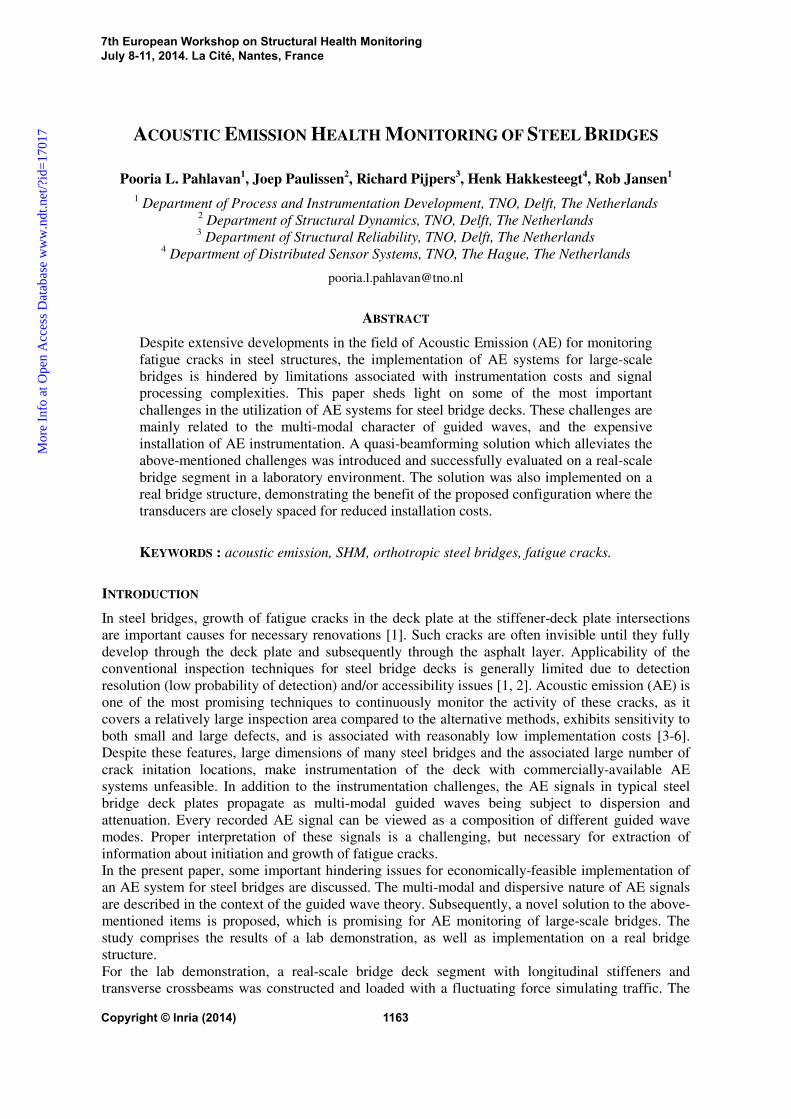
AE signals are generated by a rapid release of energy from localized sources within a material and travel through the structure. The amplitude of an AE signal is determined by geometrical spreading, material attenuation, wave dispersion, and possible structural discontinuities on its way from the AE source, e.g. active crack, to the AE sensors. These attenuation factors, when accompanied by traffic and weather-related noise, make it often impossible to detect an AE signal beyond a few meters of propogation. In thin-walled metallic structures, the AE signals can be described by a combination of different guided wave modes characterized by the dispersion curves. The fundamental symmetric (S0) and antisymmetric (A0) Lamb waves are often the dominant modes in flat plates and have the largest contribution in the acquired AE signals. The phase-speed and group-speed dispersion curves for a steel plate with 12 mm thickness have been shown in Figure 1.
0 50 100 150 200 250 300
0
1
2
3
4
5
6
7
frequency f (kHz)
phas
e sp
eed
cp
(km
/s)
S0
SH0
A0
0 50 100 150 200 250 300
0
1
2
3
4
5
6
7
frequency f (kHz)
gro
up s
pee
d c
g
(km
/s)
S0
SH0
A0
Figure 1. The dispersion curves for a 12 mm thick steel plate: phase speed (left), and group speed (right).
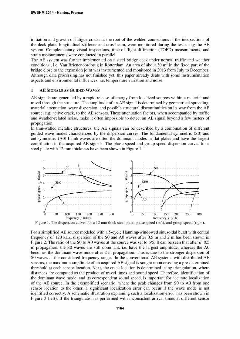
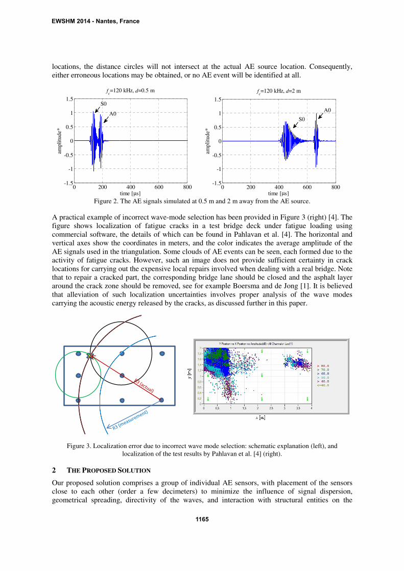
For a simplified AE source modeled with a 5-cycle Hanning-windowed sinusoidal burst with central frequency of 120 kHz, dispersion of the S0 and A0 waves after 0.5 m and 2 m has been shown in Figure 2. The ratio of the S0 to A0 waves at the source was set to 6/5. It can be seen that after d=0.5 m propagation, the S0 waves are still dominant, i.e. have the largest amplitude, whereas the A0 becomes the dominant wave mode after 2 m propagation. This is due to the stronger dispersion of S0 waves at the considered frequency range. In the conventional AE systems with distributed AE sensors, the maximum amplitude of an acquired AE signal is sought upon crossing a pre-determined threshold at each sensor location. Next, the crack location is determined using triangulation, where distances are computed as the product of travel times and sound speed. Therefore, identification of the dominant wave mode, and its correspondent sound speed, is important for accurate localization of the AE source. In the exemplified scenario, where the peak changes from S0 to A0 from one sensor location to the other, a significant localization error can occur if the wave mode is not identified correctly. A schematic illustration explaining such a localization error has been shown in Figure 3 (left). If the triangulation is performed with inconsistent arrival times at different sensor
EWSHM 2014 - Nantes, France
1164
locations, the distance circles will not intersect at the actual AE source location. Consequently, either erroneous locations may be obtained, or no AE event will be identified at all.
0 200 400 600 800-1.5
-1
-0.5
0
0.5
1
1.5
time [µs]
ampl
itud
e*
fc=120 kHz, d=0.5 m
S0
A0
0 200 400 600 800
-1.5
-1
-0.5
0
0.5
1
1.5
time [µs]
amp
litu
de*
fc=120 kHz, d=2 m
A0
S0
Figure 2. The AE signals simulated at 0.5 m and 2 m away from the AE source.
A practical example of incorrect wave-mode selection has been provided in Figure 3 (right) [4]. The figure shows localization of fatigue cracks in a test bridge deck under fatigue loading using commercial software, the details of which can be found in Pahlavan et al. [4]. The horizontal and vertical axes show the coordinates in meters, and the color indicates the average amplitude of the AE signals used in the triangulation. Some clouds of AE events can be seen, each formed due to the activity of fatigue cracks. However, such an image does not provide sufficient certainty in crack locations for carrying out the expensive local repairs involved when dealing with a real bridge. Note that to repair a cracked part, the corresponding bridge lane should be closed and the asphalt layer around the crack zone should be removed, see for example Boersma and de Jong [1]. It is believed that alleviation of such localization uncertainties involves proper analysis of the wave modes carrying the acoustic energy released by the cracks, as discussed further in this paper.
Figure 3. Localization error due to incorrect wave mode selection: schematic explanation (left), and localization of the test results by Pahlavan et al. [4] (right).
2 THE PROPOSED SOLUTION
Our proposed solution comprises a group of individual AE sensors, with placement of the sensors close to each other (order a few decimeters) to minimize the influence of signal dispersion, geometrical spreading, directivity of the waves, and interaction with structural entities on the
EWSHM 2014 - Nantes, France
1165
measurements. A specific beamforming formulation based on the guided waves characteristics and the arrival times obtained from the AE signals has been derived for localization of the AE source, in which the speed of the waves is also estimated, in contrast with the conventional beamforming AE where it is assumed to be known [7, 8]. For every set of waveforms recorded at the sensor locations, the most plausible wave mode is identified in an optimization routine in accordance with the dispersion curves for the structural component under investigation. This formulation will be referred to as quasi-beamforming (QBF) in the remainder of this paper. Once a set of signals is collected by the AE sensors upon crossing a predefined threshold, the relative arrival times are extracted by means of cross-correlation subsequent to band-pass filtering of the raw signals. If the signal recorded at sensor location j is denoted by Sj, the differential arrival time is calculated as:
ˆ ˆarg max ( ) ( )ij j i
t S t S t dtτ
τ∈ ∞
∆ = +∫ℝ
(1)
where ||·||∞ indicates the maximum norm, and the ‘hat’ sign denotes band-pass filtering. The QBF is formulated to identify the dominant wave mode and the AE source location in accordance with the minimization problem:
( ) 0 0, ,
arg min , , , , , [1,2,..., ], subject to: ( , ) and [ ( ), ( )]g
c c g ij g S Ax y c
F x y c t i j n x y c c cω ω∆ ∀ ∈ ∈ Ω ∈ (2)
where xc and yc denote the coordinates of the AE source in the plane of geometry, cg is the speed of the dominant wave mode, Ω is the physical domain under inspection, cS0 and cA0 are the group speeds of the fundamental guided wave modes S0 and A0 as functions of frequency ω, and F is the generic functional form of the error function associated with the assumed combination of the source location, speed of the dominant wave mode, and the identified arrival times from Equation (1).
3 LAB EXPERIMENTS
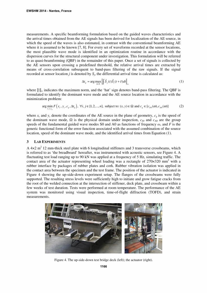
A 4×2 m2 12 mm-thick steel plate with 6 longitudinal stiffeners and 3 transverse crossbeams, which is referred to as ‘the breadboard’ hereafter, was instrumented with acoustic sensors, see Figure 4. A fluctuating test load ranging up to 90 kN was applied at a frequency of 5 Hz, simulating traffic. The contact area of the actuator representing wheel loading was a rectangle of 270×320 mm2 with a rubber interface by packages of rubber plates and cork. Rubber vibration isolation was applied in the contact area between the specimen and the test frame. The position of the actuator is indicated in Figure 4 showing the up-side-down experiment setup. The flanges of the crossbeams were fully supported. The resulting stress levels were sufficiently high to initiate and grow fatigue cracks from the root of the welded connection at the intersection of stiffener, deck plate, and crossbeam within a few weeks of test duration. Tests were performed at room temperature. The performance of the AE system was monitored using visual inspection, time-of-flight diffraction (TOFD), and strain measurements.
Figure 4. The up-side-down test bridge deck (left); the actuator (right).
EWSHM 2014 - Nantes, France
1166
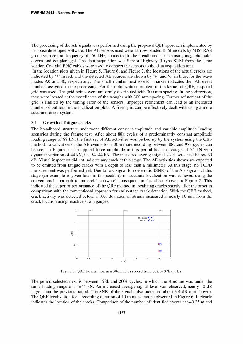
The processing of the AE signals was performed using the proposed QBF approach implemented by in-house developed software. The AE sensors used were narrow-banded R15I models by MISTRAS group with central frequency of 150 kHz, connected to the breadboard surface using magnetic hold-downs and couplant gel. The data acquisition was Sensor Highway II type SRM from the same vendor. Co-axial BNC cables were used to connect the sensors to the data acquisition unit In the location plots given in Figure 5, Figure 6, and Figure 7, the locations of the actual cracks are indicated by ‘*’ in red, and the detected AE sources are shown by ‘+’ and ‘o’ in blue, for the wave modes A0 and S0, respectively. The small number next to each marker indicates the ‘AE event number’ assigned in the processing. For the optimization problem in the kernel of QBF, a spatial grid was used. The grid points were uniformly distributed with 300 mm spacing. In the y-direction, they were located at the coordinates of the troughs with 300 mm spacing. Further refinement of the grid is limited by the timing error of the sensors. Improper refinement can lead to an increased number of outliers in the localization plots. A finer grid can be effectively dealt with using a more accurate sensor system.
3.1 Growth of fatigue cracks
The breadboard structure underwent different constant-amplitude and variable-amplitude loading scenarios during the fatigue test. After about 88k cycles of a predominantly constant amplitude loading range of 88 kN, the first set of AE activities was picked up by the system using the QBF method. Localization of the AE events for a 30-minute recording between 88k and 97k cycles can be seen in Figure 5. The applied force amplitude in this period had an average of 54 kN with dynamic variation of 44 kN, i.e. 54±44 kN. The measured average signal level was just below 30 dB. Visual inspection did not indicate any crack at this stage. The AE activities shown are expected to be emitted from fatigue cracks with a depth of less than a millimeter. At this stage, no TOFD measurement was performed yet. Due to low signal to noise ratio (SNR) of the AE signals at this stage (an example is given later in this section), no accurate localization was achieved using the conventional approach (commercial software) consequent to the effect shown in Figure 2. This indicated the superior performance of the QBF method in localizing cracks shortly after the onset in comparison with the conventional approach for early-stage crack detection. With the QBF method, crack activity was detected before a 10% deviation of strains measured at nearly 10 mm from the crack location using resistive strain gauges.
0 0.5 1 1.5 2 2.5 3 3.5 40
0.5
1
1.5
2
x [m]
y [m
]
CB[A] CB[B] CB[C]
T1
T2
T3
T4
T5
T6
5 6
7 8
8528
8562
8664
90769077
10485
2231728625
Figure 5. QBF localization in a 30-minutes record from 88k to 97k cycles.
The period selected next is between 198k and 200k cycles, in which the structure was under the same loading range of 54±44 kN. An increased average signal level was observed, nearly 10 dB larger than the previous period. The SNR of the signals also increased about 3-4 dB (not shown). The QBF localization for a recording duration of 10 minutes can be observed in Figure 6. It clearly indicates the location of the cracks. Comparison of the number of identified events at y=0.25 m and
QBF sensor group
EWSHM 2014 - Nantes, France
1167
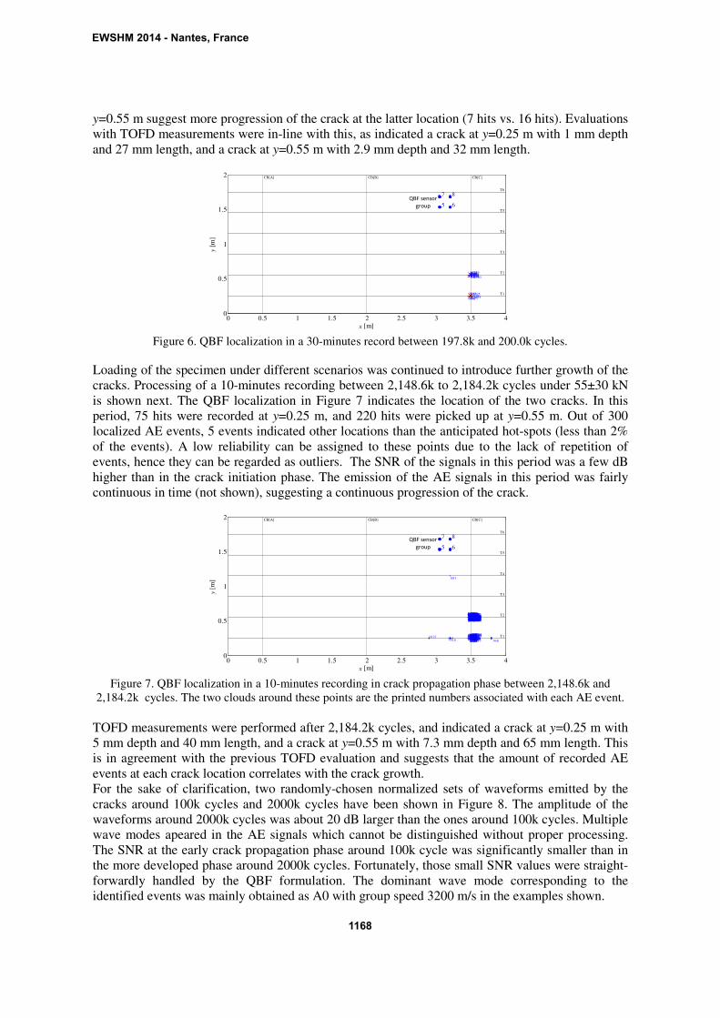
y=0.55 m suggest more progression of the crack at the latter location (7 hits vs. 16 hits). Evaluations with TOFD measurements were in-line with this, as indicated a crack at y=0.25 m with 1 mm depth and 27 mm length, and a crack at y=0.55 m with 2.9 mm depth and 32 mm length.
0 0.5 1 1.5 2 2.5 3 3.5 40
0.5
1
1.5
2
x [m]
y [m
]
CB[A] CB[B] CB[C]
T1
T2
T3
T4
T5
T6
5 6
7 8
16
50
1341378261033
1039
16431658
16941695
1696
1698
1702
170317182649
3605
3699375439293932
4475
Figure 6. QBF localization in a 30-minutes record between 197.8k and 200.0k cycles.
Loading of the specimen under different scenarios was continued to introduce further growth of the cracks. Processing of a 10-minutes recording between 2,148.6k to 2,184.2k cycles under 55±30 kN is shown next. The QBF localization in Figure 7 indicates the location of the two cracks. In this period, 75 hits were recorded at y=0.25 m, and 220 hits were picked up at y=0.55 m. Out of 300 localized AE events, 5 events indicated other locations than the anticipated hot-spots (less than 2% of the events). A low reliability can be assigned to these points due to the lack of repetition of events, hence they can be regarded as outliers. The SNR of the signals in this period was a few dB higher than in the crack initiation phase. The emission of the AE signals in this period was fairly continuous in time (not shown), suggesting a continuous progression of the crack.
0 0.5 1 1.5 2 2.5 3 3.5 40
0.5
1
1.5
2
x [m]
y [m
]
CB[A] CB[B] CB[C]
T1
T2
T3
T4
T5
T6
5 6
7 8
1 456
12
14
16171824
4352
626594
102103
112
114
123129
132
134136150158
160
164
201217218220
227248
266
269
270271276
277279285287288295299304
317
318323326
327328
341359373
377
414430
434474481 496497504509
517
519
536558574
582603618
681
693
707790808
824845857862
865882
940
9481057
108310911099
12111269
12711308
13531372
14441456
1471
15331535
1547
1595
1599
1605
1615
16871707
1715
17521760
1774
180118051807
1811
1819
1821
18231835
18431851
18571882
1886
1928
19651977
1989
1995
1997
2043
20592195
22982353
23562357
2359
23652367
2370
241424352441244324592462
2490
26112625
2635
26362639264126902692
26952698
2720
274627562757
2772
27782792
2814
2817
282128222825
2830
2834283528402843
28442850
28592868
2869
28772879
2881
28832884294329443026302730713077
3079
3082
32473319
33523355335633603362
33723401
3403
3412342434273460
346834703499
3518
3557
3558
35593573
3574
35793586
359635983611
362336563657365836693670
367236733679
36803681368436863687370637083709
3711
3717372337253728
3737375637903800
3802
3804
3806
38713876
387738793883
38853894
3976
3979398039813990
3991
39923994
3996
40024004
4021402541024127
4150
4192
41964201
42044206
423142324246
43384341
4368
43724379
43804445
444744534470
448847504834
Figure 7. QBF localization in a 10-minutes recording in crack propagation phase between 2,148.6k and
2,184.2k cycles. The two clouds around these points are the printed numbers associated with each AE event.
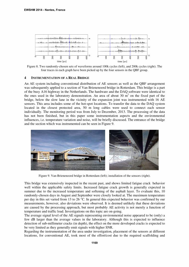
TOFD measurements were performed after 2,184.2k cycles, and indicated a crack at y=0.25 m with 5 mm depth and 40 mm length, and a crack at y=0.55 m with 7.3 mm depth and 65 mm length. This is in agreement with the previous TOFD evaluation and suggests that the amount of recorded AE events at each crack location correlates with the crack growth. For the sake of clarification, two randomly-chosen normalized sets of waveforms emitted by the cracks around 100k cycles and 2000k cycles have been shown in Figure 8. The amplitude of the waveforms around 2000k cycles was about 20 dB larger than the ones around 100k cycles. Multiple wave modes apeared in the AE signals which cannot be distinguished without proper processing. The SNR at the early crack propagation phase around 100k cycle was significantly smaller than in the more developed phase around 2000k cycles. Fortunately, those small SNR values were straight-forwardly handled by the QBF formulation. The dominant wave mode corresponding to the identified events was mainly obtained as A0 with group speed 3200 m/s in the examples shown.
QBF sensor group
QBF sensor group
EWSHM 2014 - Nantes, France
1168
02
4
0
100
200
300
400
500
600
time [µs]
02
4
0
100
200
300
400
500
600
time [µs]
µ
time [µs] time [µs]
Figure 8. Two randomly-chosen sets of waveforms around 100k cycles (left), and 200k cycles (right). The four traces in each graph have been picked up by the four sensors in the QBF group.
4 INSTRUMENTATION OF A REAL BRIDGE
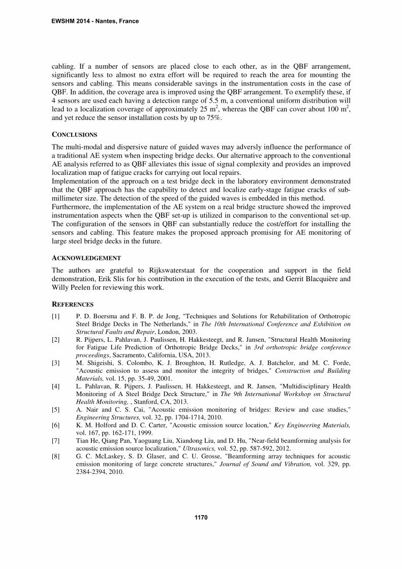
An AE system including conventional distribution of AE sensors as well as the QBF arrangement was subsequently applied to a section of Van Brienenoord bridge in Rotterdam. This bridge is a part of the busy A16 highway in the Netherlands. The hardware and the DAQ software were identical to the ones used in the laboratory demonstration. An area of about 30 m2 on the fixed part of the bridge, below the slow lane in the vicinity of the expansion joint was instrumented with 16 AE sensors. This area includes some of the hot-spot locations. To transfer the data to the DAQ system located in the closest protected area, 50 m long cables were used to connect each sensor individually. The monitoring period was from July to December, 2013. The processing of the data has not been finished, but in this paper some instrumentation aspects and the environmental influences, i.e. temperature variation and noise, will be briefly discussed. The entrance of the bridge and the section which was instrumented can be seen in Figure 9.
Figure 9. Van-Brienenoord bridge in Rotterdam (left); installation of the sensors (right).
This bridge was extensively inspected in the recent past, and shows limited fatigue crack behavior well within the applicable safety limits. Increased fatigue crack growth is generally expected in summer due to the increased temperature and softening of the asphalt layer. To evaluate this, 10 randomly-chosen days in August and September were closely looked at. The maximum temperature per day in this set varied from 13 to 26 °C. In general this expected behavior was confirmed by our measurements, however, also deviations were observed. It is deemed unlikely that these deviations are caused by the processing approach, but most probably AE activity is not merely a function of temperature and traffic load. Investigations on this topic are on-going. The average signal level of the AE signals representing environmental noise appeared to be (only) a few dB larger than the average values in the laboratory. Although this is expected to influence detection of sub-millimeter cracks (in depth), the effect on the more developed cracks is expected to be very limited as they generally emit signals with higher SNR. Regarding the instrumentation of the area under investigation, placement of the sensors at different locations, for conventional AE, took most of the effort/cost due to the required scaffolding and
EWSHM 2014 - Nantes, France
1169
cabling. If a number of sensors are placed close to each other, as in the QBF arrangement, significantly less to almost no extra effort will be required to reach the area for mounting the sensors and cabling. This means considerable savings in the instrumentation costs in the case of QBF. In addition, the coverage area is improved using the QBF arrangement. To exemplify these, if 4 sensors are used each having a detection range of 5.5 m, a conventional uniform distribution will lead to a localization coverage of approximately 25 m2, whereas the QBF can cover about 100 m2, and yet reduce the sensor installation costs by up to 75%.
CONCLUSIONS
The multi-modal and dispersive nature of guided waves may adversly influence the performance of a traditional AE system when inspecting bridge decks. Our alternative approach to the conventional AE analysis referred to as QBF alleviates this issue of signal complexity and provides an improved localization map of fatigue cracks for carrying out local repairs. Implementation of the approach on a test bridge deck in the laboratory environment demonstrated that the QBF approach has the capability to detect and localize early-stage fatigue cracks of sub-millimeter size. The detection of the speed of the guided waves is embedded in this method. Furthermore, the implementation of the AE system on a real bridge structure showed the improved instrumentation aspects when the QBF set-up is utilized in comparison to the conventional set-up. The configuration of the sensors in QBF can substantially reduce the cost/effort for installing the sensors and cabling. This feature makes the proposed approach promising for AE monitoring of large steel bridge decks in the future.
ACKNOWLEDGEMENT
The authors are grateful to Rijkswaterstaat for the cooperation and support in the field demonstration, Erik Slis for his contribution in the execution of the tests, and Gerrit Blacquière and Willy Peelen for reviewing this work.
REFERENCES
[1] P. D. Boersma and F. B. P. de Jong, "Techniques and Solutions for Rehabilitation of Orthotropic Steel Bridge Decks in The Netherlands," in The 10th International Conference and Exhibition on
Structural Faults and Repair, London, 2003. [2] R. Pijpers, L. Pahlavan, J. Paulissen, H. Hakkesteegt, and R. Jansen, "Structural Health Monitoring
for Fatigue Life Prediction of Orthotropic Bridge Decks," in 3rd orthotropic bridge conference
proceedings, Sacramento, California, USA, 2013. [3] M. Shigeishi, S. Colombo, K. J. Broughton, H. Rutledge, A. J. Batchelor, and M. C. Forde,
"Acoustic emission to assess and monitor the integrity of bridges," Construction and Building
Materials, vol. 15, pp. 35-49, 2001. [4] L. Pahlavan, R. Pijpers, J. Paulissen, H. Hakkesteegt, and R. Jansen, "Multidisciplinary Health
Monitoring of A Steel Bridge Deck Structure," in The 9th International Workshop on Structural
Health Monitoring, , Stanford, CA, 2013. [5] A. Nair and C. S. Cai, "Acoustic emission monitoring of bridges: Review and case studies,"
Engineering Structures, vol. 32, pp. 1704-1714, 2010. [6] K. M. Holford and D. C. Carter, "Acoustic emission source location," Key Engineering Materials,
vol. 167, pp. 162-171, 1999. [7] Tian He, Qiang Pan, Yaoguang Liu, Xiandong Liu, and D. Hu, "Near-field beamforming analysis for
acoustic emission source localization," Ultrasonics, vol. 52, pp. 587-592, 2012. [8] G. C. McLaskey, S. D. Glaser, and C. U. Grosse, "Beamforming array techniques for acoustic
emission monitoring of large concrete structures," Journal of Sound and Vibration, vol. 329, pp. 2384-2394, 2010.
EWSHM 2014 - Nantes, France
1170