acoustic emission(발표할 때 유용할것)
TRANSCRIPT

7/31/2019 acoustic emission( )
http://slidepdf.com/reader/full/acoustic-emission- 1/82
Physical Properties during rock deformation
1. Testing machine stiffness
2. Pre- and post-peak behaviour3. Volume changes (volumetric strain)
4. Elastic wave speeds
5. Acoustic emission
Tuesday, April 19, 2011

7/31/2019 acoustic emission( )
http://slidepdf.com/reader/full/acoustic-emission- 2/82
1. Testing machine stiffness (and other corrections)
Low machine stiffness -k High machine stiffness -k
k
The first important correction is for the deformation of the loading machine itself:
- sample is usually much more compressible (less still) so dominates- but even so, for frame of low stiffness, an apparent lower modulus will be measured
Tuesday, April 19, 2011

7/31/2019 acoustic emission( )
http://slidepdf.com/reader/full/acoustic-emission- 3/82
Complete force-displacement curves
Especially important when comparing deformation of rocks of widely differingstiffnesses...
Tuesday, April 19, 2011

7/31/2019 acoustic emission( )
http://slidepdf.com/reader/full/acoustic-emission- 4/82
axial
Volume
Dilatancy, rupture and compaction
lateral
I – phase of compaction of pores and cracks (stiffening = increase in E)
II – linear elastic phase (no change in stiffness; E = constant)
III – non-linear phase – growth of new cracks – dilatancy (E decreases)
IV – strain softening phase – cracks link up to form the shear fault
V - dynamic instability and failure – equivalent to an earthquake in the crust
VI – stable frictional sliding on the fault plane
Reminder...
This time w.r.t.lateral and
volumetric strains
Tuesday, April 19, 2011

7/31/2019 acoustic emission( )
http://slidepdf.com/reader/full/acoustic-emission- 5/82
Sample shortening (Vp/Vs/AE)
Another calibration is the natural ‘shortening’ of the sample. This will lead toelastic wave velocities higher than they should be. Measure via LVDT vs. pressure
Tuesday, April 19, 2011
7/31/2019 acoustic emission( )
http://slidepdf.com/reader/full/acoustic-emission- 6/82
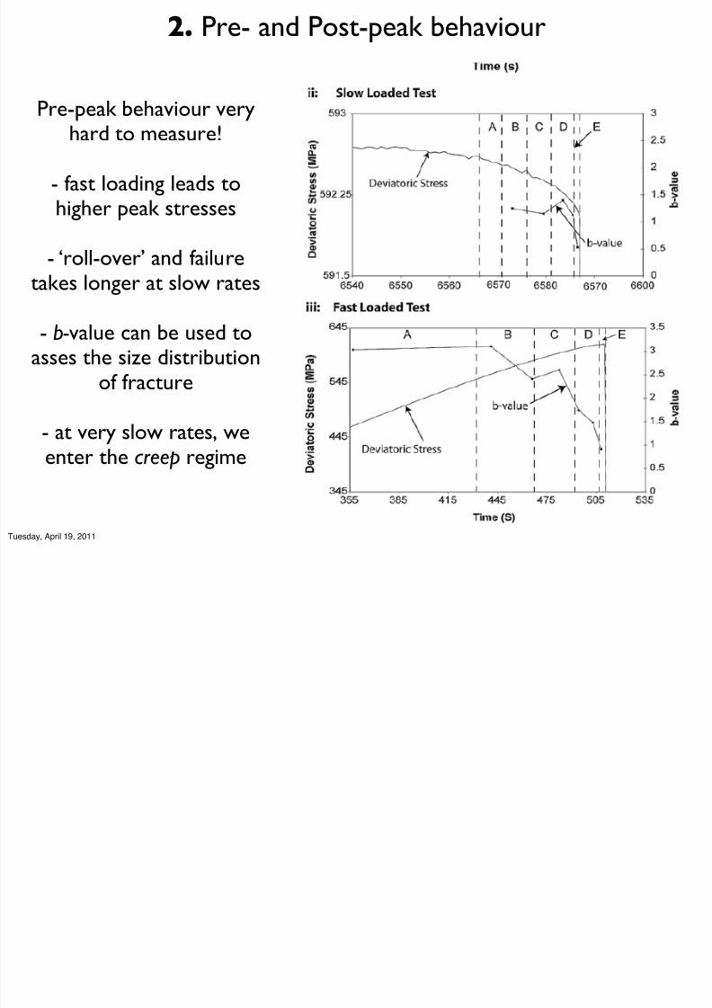
2. Pre- and Post-peak behaviour
Pre-peak behaviour veryhard to measure!
- fast loading leads tohigher peak stresses
- ‘roll-over’ and failuretakes longer at slow rates
- b-value can be used toasses the size distribution
of fracture
- at very slow rates, weenter the creep regime
Tuesday, April 19, 2011

7/31/2019 acoustic emission( )
http://slidepdf.com/reader/full/acoustic-emission- 7/82
Increasingconfinement increasesstrength, as well as thepost peak behaviour:
brittle -> cataclasis
Another example of
increasing strain rateincreasing the
apparent strength of the rock...
Pre- and Post-peak behaviour
Tuesday, April 19, 2011

7/31/2019 acoustic emission( )
http://slidepdf.com/reader/full/acoustic-emission- 8/82
Use AE as a feedback... slow the process
Solution championed by lockner (USGS) was to slow the process by using afeedback from the AE itself, converted to a voltage. This way, strain is variable.
Tuesday, April 19, 2011

7/31/2019 acoustic emission( )
http://slidepdf.com/reader/full/acoustic-emission- 9/82
Use AE as a feedback... slow the process
Solution championed by lockner (USGS) was to slow the process by using afeedback from the AE itself, converted to a voltage. This way, strain is variable.
Tuesday, April 19, 2011

7/31/2019 acoustic emission( )
http://slidepdf.com/reader/full/acoustic-emission- 10/82
Post-peak behaviour is investigated through
‘cyclic’ means to keep the sample intact...
Tuesday, April 19, 2011

7/31/2019 acoustic emission( )
http://slidepdf.com/reader/full/acoustic-emission- 11/82
...Both axial and radial cycles show the same
effect of decreasing stiffness with time
Tuesday, April 19, 2011

7/31/2019 acoustic emission( )
http://slidepdf.com/reader/full/acoustic-emission- 12/82
Anisotropy
Normal to bed parallel to bed
Deformation of Takidani granite (Japan Alps) normal and parallel to jointing
Tuesday, April 19, 2011

7/31/2019 acoustic emission( )
http://slidepdf.com/reader/full/acoustic-emission- 13/82
3. Volumetric strain
Volumetric strain,
unlike axial orradial, can give a
sense of the
changing volume of
the sample,
including thecontribution of the
cracks and pores as
they deform. In this
case, measured via
strain gauges
Tuesday, April 19, 2011

7/31/2019 acoustic emission( )
http://slidepdf.com/reader/full/acoustic-emission- 14/82
Alternatives, use
the servo-
controlled pore
pressure system
to receive the
pore fluid atconstant
pressure, thus
measuring
volumetric strain
vie the volume of water expelled
from the cracks
Volumetric strain
Tuesday, April 19, 2011

7/31/2019 acoustic emission( )
http://slidepdf.com/reader/full/acoustic-emission- 15/82
Volume change
AxialMean
Radial
A
B
C D i f f e r e n t i a l S t r
e s s ( M P a )
Axial Strain (fractional)
Time from start (s)
P - w a v e
V e l o c i t y ( m / s )
V o l u m
e c h a n g e ( ml )
C u m
u l a t i v e A E ( h i t s )
AE Hit rate
0
100
200
300
400
-1
-0.5
0
0.5
1
0
100
200
300
400
500
3500
4000
4500
5000
5500
6000
-0.01 -0.005 0 0.005 0.01 0.015 0.02 0.025
0
100
200
300
400
0
500
1000
1500
2000
0 1800 3600 5400
This measure
is very
sensitive to:
- pores vs.
cracks
- anisotropy
and loading
direction
- the crack
aspect ratio...
Etna basalt
(cracked)
Tuesday, April 19, 2011

7/31/2019 acoustic emission( )
http://slidepdf.com/reader/full/acoustic-emission- 16/82
• We have just seen the effect of micro-cracks have upon deformation via
volumetric strain...• Other methods are also available that give more detailed data, including
tomography.• Relies on a active system of sending a mechanical pulse through the sample
and receiving it at the other end. Typically a piezoelectric transducer is
used that converts voltage to mechanical pulses directly and vice versa.
P-wave ‘sender’
Cracked medium
P-wave ‘receiver’
Mechanical pulse in:
Traveling parallel to
cracks
Mechanical pulse in:
Traveling normal to
cracks
Mechanical pulse out:
Time taken to cross sample
Gives a velocity.
Mechanical pulse out:
This time, the pulse
takes longer to be
received (Tn>Tp), and
has loweramplitude….
T0 Tp
T0 Tn
4. Elastic wave speeds
Anisotropy and wave speed...
Tuesday, April 19, 2011

7/31/2019 acoustic emission( )
http://slidepdf.com/reader/full/acoustic-emission- 17/82
Measurement of Vp/Vs and AE: Piezoelectric
Crystals and Transducers
ValpeyFisher Crystals ValpeyFisher Transducers
P-Wave crystal signal output S-Wave crystal signal output
Relatively new (~25 years) development...
Tuesday, April 19, 2011

7/31/2019 acoustic emission( )
http://slidepdf.com/reader/full/acoustic-emission- 18/82
Measurement of Vp/Vs and AE: set-up
- A pulse generator sends volt spikes (usually square waves of short
duration) to the transducer, and simultaneously a ‘trigger is sent to therecording device to tell it when the pulse was sent
- The transducer active element is excited and sends a mechanical pulseacross a specimen, where it is received by a second identical sensor
- The mechanical signal is converted into electrical voltage.-The voltage is first amplified, by 20/40/40 dB (x10/100/1000) depending on
the rock material, distance, etc.-The oscilloscope records the received pulse, as well as the start time from
the trigger.
Tuesday, April 19, 2011

7/31/2019 acoustic emission( )
http://slidepdf.com/reader/full/acoustic-emission- 19/82
Picking the arrival time:
P-wave
Tuesday, April 19, 2011
7/31/2019 acoustic emission( )
http://slidepdf.com/reader/full/acoustic-emission- 20/82
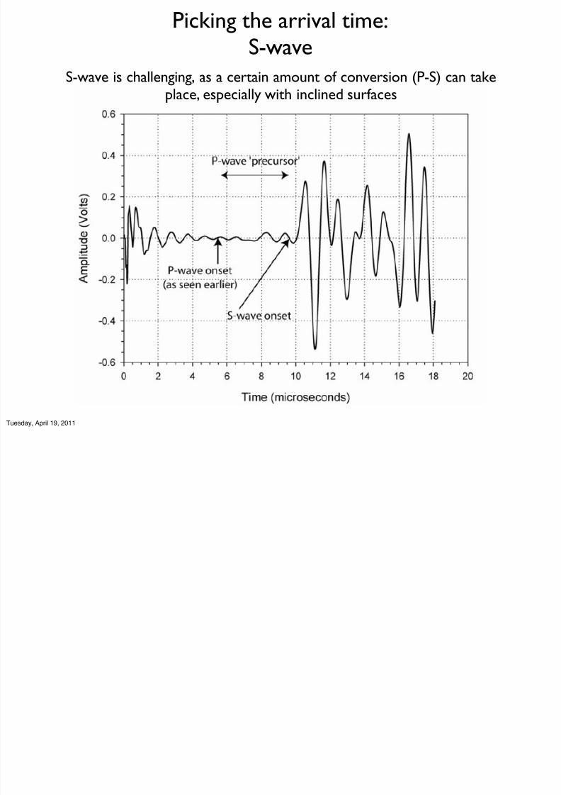
Picking the arrival time:
S-wave
S-wave is challenging, as a certain amount of conversion (P-S) can take
place, especially with inclined surfaces
Tuesday, April 19, 2011

7/31/2019 acoustic emission( )
http://slidepdf.com/reader/full/acoustic-emission- 21/82
Applications:
P-wave and S-wave anisotropy
In this example, the P-wave velocity wasmeasured as a functionof radial angle aroundthe edge of a cylindrical
core
For visible layering in asedimentary rock type(shown here) there is apronounced anisotropy
Important for manyareas of Geoscience...oil, gas exploration,seismic tomography,exploration...
Bentheimsandstone,
porosity ~23%
Tuesday, April 19, 2011

7/31/2019 acoustic emission( )
http://slidepdf.com/reader/full/acoustic-emission- 22/82
Same rock type, but thistime water saturated.
As water has a higherP-wave velocity that air,the bulk velocity is
higher
Applications:
P-wave and S-wave anisotropy
Tuesday, April 19, 2011

7/31/2019 acoustic emission( )
http://slidepdf.com/reader/full/acoustic-emission- 23/82
Applications:
P-wave and S-wave variation with isostatic pressure
Another important
application
Crucial for
interpreting seismicdata where we wishto know the velocityof the propagating
medium at differentburial depths, e.g.
deep subductionzones, exploration,etc.
Tuesday, April 19, 2011

7/31/2019 acoustic emission( )
http://slidepdf.com/reader/full/acoustic-emission- 24/82
Applications:
P-wave and S-wave variation with isostatic pressure
Another importantapplication.
Different rock type...
‘Crab orchard
sandstone’ withporosity of only 4%
Tuesday, April 19, 2011

7/31/2019 acoustic emission( )
http://slidepdf.com/reader/full/acoustic-emission- 25/82
Applications:
P-wave and S-wave variation with isostatic pressure
Takidanigranite,porosity ~1%
Tuesday, April 19, 2011
A l

7/31/2019 acoustic emission( )
http://slidepdf.com/reader/full/acoustic-emission- 26/82
Applications:
P-wave and S-wave anisotropy with isostatic pressure
By measuring the fabric of the rocks, and examining the fast and slow velocity
planes, we can establish the degree of anisotropy (more on Thursday)
Tuesday, April 19, 2011
A l

7/31/2019 acoustic emission( )
http://slidepdf.com/reader/full/acoustic-emission- 27/82
Applications:
P-wave and S-wave anisotropy with isostatic pressure
By measuring the fabric of the rocks, and examining the fast and slow velocity
planes, we can establish the degree of anisotropy (more on Thursday)
Tuesday, April 19, 2011
A li i

7/31/2019 acoustic emission( )
http://slidepdf.com/reader/full/acoustic-emission- 28/82
Applications:
P-wave and S-wave anisotropy with isostatic pressure
By measuring the fabric of the rocks, and examining the fast and slow velocity
planes, we can establish the degree of anisotropy (more on Thursday)
Tuesday, April 19, 2011

7/31/2019 acoustic emission( )
http://slidepdf.com/reader/full/acoustic-emission- 29/82
Influence of crack shape
Vp : Influence shape of porosity
What causes anisotropybesides the sedimentary
fabric?
- Cracks
- Pores
- Crystallographicpreferred orientation
- Lattice preferredorientation
Tuesday, April 19, 2011
fl f

7/31/2019 acoustic emission( )
http://slidepdf.com/reader/full/acoustic-emission- 30/82
Influence of crack shape
Vp : Influence shape of porosity
What causes anisotropybesides the sedimentary
fabric?
- Cracks
- Pores
- Crystallographicpreferred orientation
- Lattice preferredorientation
Closing a ‘crack’ requiresless pressure than a
‘pore’. Key parameter:
aspect ratio
Tuesday, April 19, 2011
I fl f k h

7/31/2019 acoustic emission( )
http://slidepdf.com/reader/full/acoustic-emission- 31/82
Influence of crack shape
Vp : Influence shape of porosity
By considering the degree, alignment, and density of ‘penny shaped’ cracks, atheoretical framework can be derived, allowing a comparison to the laboratorydata to be made in terms of the degree of contribution to the anisotropy
Schubnel, Benson et al., 2006
Tuesday, April 19, 2011
V f k d d

7/31/2019 acoustic emission( )
http://slidepdf.com/reader/full/acoustic-emission- 32/82
Variation of crack density and
aspect ratio with pressure
Schubnel, Benson et al., 2006
Using those Vp and Vs data, which can be linked theoretically to the crack network via a non-interactive effective medium model (Kachanov, 1994), one can, forexample, invert the velocity for the changing microstructural parameters:
Tuesday, April 19, 2011

7/31/2019 acoustic emission( )
http://slidepdf.com/reader/full/acoustic-emission- 33/82
Examination of the microstructure reveals
the classic ‘pores vs. cracks’ argument!
Tuesday, April 19, 2011

7/31/2019 acoustic emission( )
http://slidepdf.com/reader/full/acoustic-emission- 34/82
Examination of the microstructure reveals
the classic ‘pores vs. cracks’ argument!
Somewhat off-topic... Mercury injection porosimetry alsogenerates data to support this hypothesis:
Tuesday, April 19, 2011
C bi V k

7/31/2019 acoustic emission( )
http://slidepdf.com/reader/full/acoustic-emission- 35/82
In all cases:
- Velocity increases withPressure
- Crack density decreaseswith pressure
- aspect ratio increases
But with very different
relative responses withrespect to the balancebetween ‘pores’ and ‘cracks’as well as the anisotropy of the rock
Combine Vp, crack
density, and aspect ratio
Tuesday, April 19, 2011
Influence of fluid bulk modulus
7/31/2019 acoustic emission( )
http://slidepdf.com/reader/full/acoustic-emission- 36/82
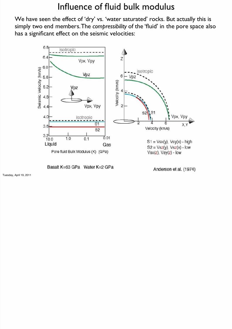
Influence of fluid bulk modulus
We have seen the effect of ‘dry’ vs. ‘water saturated’ rocks. But actually this issimply two end members. The compressibility of the ‘fluid’ in the pore space alsohas a significant effect on the seismic velocities:
Tuesday, April 19, 2011
S k di t ib ti l ti l iti

7/31/2019 acoustic emission( )
http://slidepdf.com/reader/full/acoustic-emission- 37/82
Summary: crack distributions vs. elastic wave velocities(also see Zimmerman ‘Compressibility of sandstones’ for a good review)
Tuesday, April 19, 2011
5 Acoustic emissions
7/31/2019 acoustic emission( )
http://slidepdf.com/reader/full/acoustic-emission- 38/82
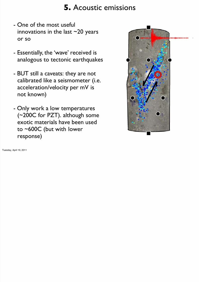
5. Acoustic emissions
- One of the most usefulinnovations in the last ~20 yearsor so
- Essentially, the ‘wave’ received isanalogous to tectonic earthquakes
- BUT still a caveats: they are notcalibrated like a seismometer (i.e.acceleration/velocity per mV isnot known)
- Only work a low temperatures(~200C for PZT). although someexotic materials have been usedto ~600C (but with lowerresponse)
Tuesday, April 19, 2011
Acoustic Emission

7/31/2019 acoustic emission( )
http://slidepdf.com/reader/full/acoustic-emission- 39/82
• Acoustic emissions (AEs) are high frequency (100 kHz – 5 MHz) strain waves.
• Emitted by rapid strain events: cracking, phase transformations, etc.
• They are the laboratory analogue for seismic events in the crust.
• Schematic of a received AEwaveform (known as a hit ).
• We measure specificparameters of each AE hit:• Amplitude threshold• Onset time• Rise time• Duration• Peak amplitude• Energy
• We also measure the hitrate and cumulative hits.
• We look at hit statistics.• We use multiple
transducers to locate thesources of AE events in 3D.
Acoustic Emission
Tuesday, April 19, 2011
Acoustic Emission location

7/31/2019 acoustic emission( )
http://slidepdf.com/reader/full/acoustic-emission- 40/82
We can alreadyfail samples inthe laboratory,and use acoustic
emission (AE) tolocate the faultproduced usingminiature piezo-electric sensors
Lab setup
Schematic
‘Microseismic’
(AE) event
‘Fault’
LOAD
To measurement and dataanalysis equipment…
Miniature
‘Sensor’
Acoustic Emission location
Tuesday, April 19, 2011
Acoustic Emission location

7/31/2019 acoustic emission( )
http://slidepdf.com/reader/full/acoustic-emission- 41/82
Acoustic Emission location
First pioneered by Lockner, Byerlee, and others at the USGS in the 80’s and
90’s (during the last bug Rock physic ‘push into understanding earthquakes
Tuesday, April 19, 2011
Acoustic Emission location
7/31/2019 acoustic emission( )
http://slidepdf.com/reader/full/acoustic-emission- 42/82
Acoustic Emission location
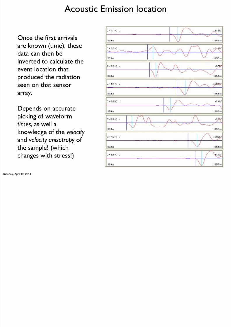
Once the first arrivals
are known (time), these
data can then be
inverted to calculate the
event location that
produced the radiation
seen on that sensorarray.
Depends on accurate
picking of waveform
times, as well aknowledge of the velocity
and velocity anisotropy of
the sample! (which
changes with stress!)
Tuesday, April 19, 2011
Acoustic Emission location

7/31/2019 acoustic emission( )
http://slidepdf.com/reader/full/acoustic-emission- 43/82
Acoustic Emission location
Tuesday, April 19, 2011
Acoustic Emission location

7/31/2019 acoustic emission( )
http://slidepdf.com/reader/full/acoustic-emission- 44/82
0
100
200
300
400
500
600
0
2000
4000
6000
8000
10000
12000
16:18:00 16:18:30 16:19:00 16:19:30
S t r e s s ,
M P a
Hi t r a t e ,1 / s
Time, H:M:S
Acoustic Emission location
Tuesday, April 19, 2011
Acoustic Emission location

7/31/2019 acoustic emission( )
http://slidepdf.com/reader/full/acoustic-emission- 45/82
0
100
200
300
400
500
600
0
2000
4000
6000
8000
10000
12000
16:18:00 16:18:30 16:19:00 16:19:30
S t r e s s ,
M P a
Hi t r a t e ,1 / s
Time, H:M:S
Acoustic Emission location
Tuesday, April 19, 2011
Acoustic Emission location

7/31/2019 acoustic emission( )
http://slidepdf.com/reader/full/acoustic-emission- 46/82
0
100
200
300
400
500
600
0
1000
2000
3000
4000
5000
6000
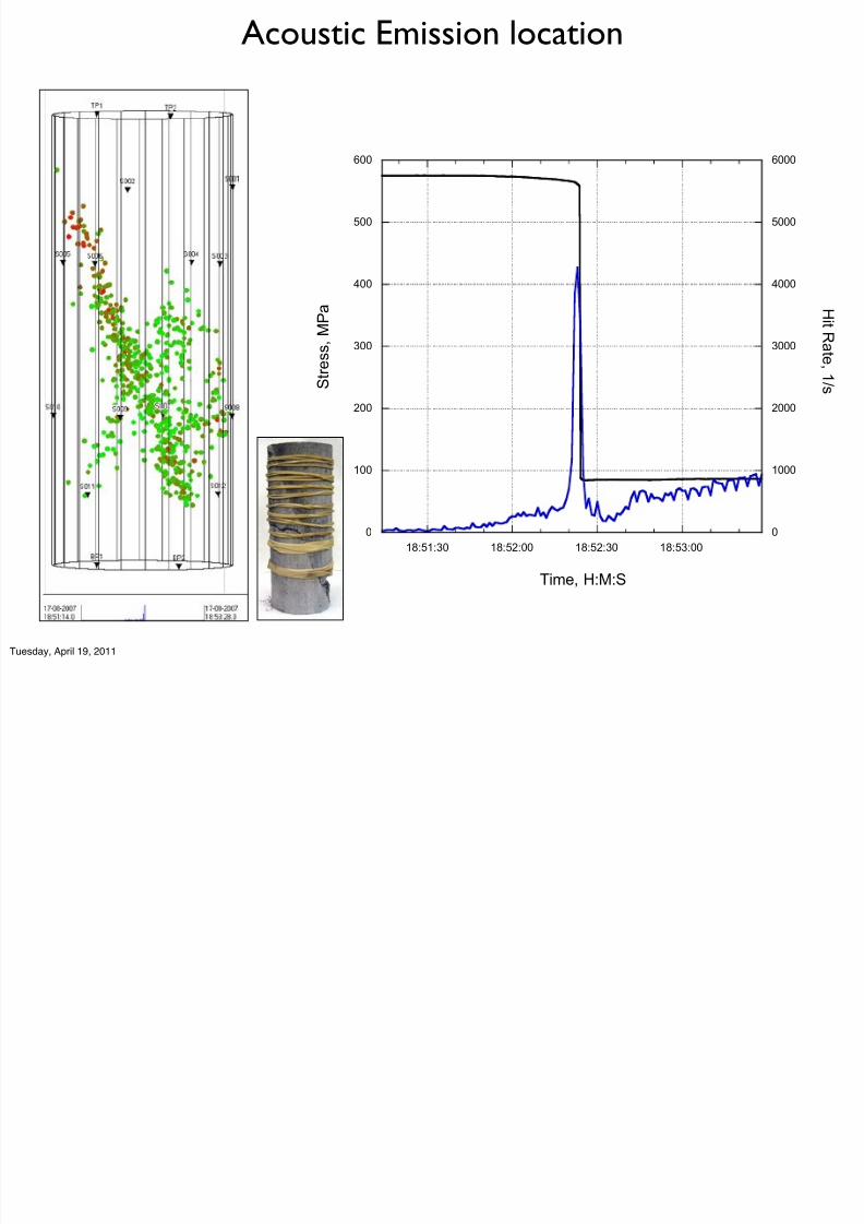
18:51:30 18:52:00 18:52:30 18:53:00
S t r e s s ,
M P a
Hi t R a t e ,1 / s
Time, H:M:S
Acoustic Emission location
Tuesday, April 19, 2011
Acoustic Emission location
7/31/2019 acoustic emission( )
http://slidepdf.com/reader/full/acoustic-emission- 47/82
0
100
200
300
400
500
600
0
1000
2000
3000
4000
5000
6000
18:51:30 18:52:00 18:52:30 18:53:00
S t r e s s ,
M P a
Hi t R a t e ,1 / s
Time, H:M:S
Acoustic Emission location
Tuesday, April 19, 2011
Acoustic Emission location

7/31/2019 acoustic emission( )
http://slidepdf.com/reader/full/acoustic-emission- 48/82
0
100
200
300
400
500
600
0
100
200
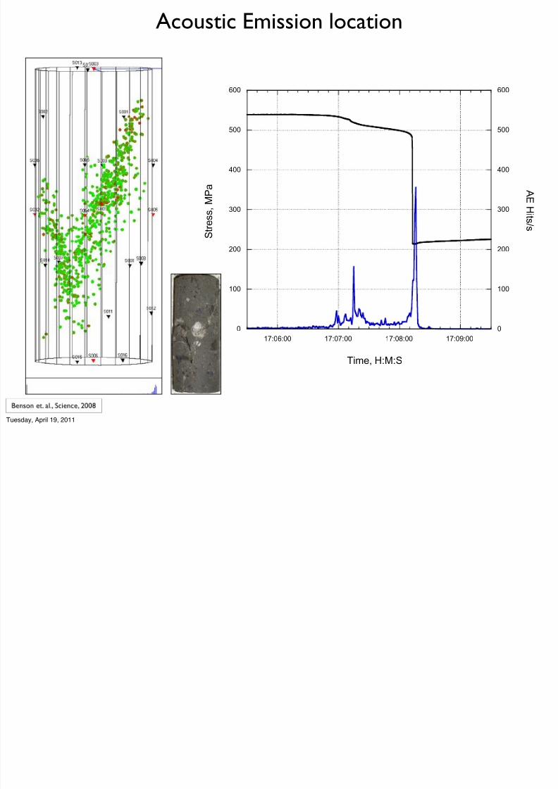
300
400
500
600
17:06:00 17:07:00 17:08:00 17:09:00
S t r e s s , M
P a A
E Hi t s / s
Time, H:M:S
Acoustic Emission location
Tuesday, April 19, 2011
Acoustic Emission location
7/31/2019 acoustic emission( )
http://slidepdf.com/reader/full/acoustic-emission- 49/82
0
100
200
300
400
500
600
0
100
200
300
400
500
600
17:06:00 17:07:00 17:08:00 17:09:00
S t r e s s , M
P a A
E Hi t s / s
Time, H:M:S
Acoustic Emission location
Tuesday, April 19, 2011

7/31/2019 acoustic emission( )
http://slidepdf.com/reader/full/acoustic-emission- 50/82
Pick the data

7/31/2019 acoustic emission( )
http://slidepdf.com/reader/full/acoustic-emission- 51/82
Pick the data...
Tuesday, April 19, 2011
Pick the data

7/31/2019 acoustic emission( )
http://slidepdf.com/reader/full/acoustic-emission- 52/82
Pick the data...
Window
‘Pick’
Function
Tuesday, April 19, 2011
Source location methods and accuracy

7/31/2019 acoustic emission( )
http://slidepdf.com/reader/full/acoustic-emission- 53/82
Source location methods and accuracy
Everyone expects good accuracy (they believe what theysee!). But...
Main factors:
• Picked arrival times (random error)• Velocity model (systematic error)
Also:
• Sensor array is important (3D distribution, and surveyedlocations
• Source location method
Main criteria... time residuals
Tuesday, April 19, 2011
Source location methods and accuracy

7/31/2019 acoustic emission( )
http://slidepdf.com/reader/full/acoustic-emission- 54/82
Source location methods and accuracy
• Direct Grid Search methods
• Standard iterative methods
• Simplex
• Geiger
• Other methods:
• Joint hypocentre
• Relative location
• Genetic algorithms
Some of these better than others... usuallyinvolving analytical vs. computational (iterativeapproaches). Computing is cheaper these days so...
Tuesday, April 19, 2011
Source location methods and accuracy

7/31/2019 acoustic emission( )
http://slidepdf.com/reader/full/acoustic-emission- 55/82
Source location methods and accuracy
Tuesday, April 19, 2011
Source location methods and accuracy

7/31/2019 acoustic emission( )
http://slidepdf.com/reader/full/acoustic-emission- 56/82
Source location methods and accuracy
Tuesday, April 19, 2011
Simplex and Geiger methods

7/31/2019 acoustic emission( )
http://slidepdf.com/reader/full/acoustic-emission- 57/82
Simplex and Geiger methods
Solving for:
θ=(t0, x0, y 0, zo )
with residual:ri=ti-to-Ti(x0, y 0, z0 )
where: ti = measured arrival time; Ti = calculated time
Minimizing a misfit function:
Φ(r)
The function relating the arrival times and the locationis nonlinear since there is no single step approach to
find the best event location.Tuesday, April 19, 2011
Geiger method

7/31/2019 acoustic emission( )
http://slidepdf.com/reader/full/acoustic-emission- 58/82
Geiger method
Linearize the problem by saying:
θ = θ* + Δθ& Solve:
Α Δθ = r
Where A = matrix (n x 4) of partial derivatives (e.g. δTi/δx0)Matrix inversion problem, via SVD (singular valued decomposition).
Important parameters:
• ‘Tolerance’ - Repeat until Δθ < tolerance• ‘Max iterations’ - Stop if exceeded
• ‘Condition # limit’ - Stop if exceeded. SVD condition condition #is inversely proportional to the stability of the inversion
•‘Step size’ - starting step size for partial derivative calculation.
Tuesday, April 19, 2011
Simplex method

7/31/2019 acoustic emission( )
http://slidepdf.com/reader/full/acoustic-emission- 59/82
Simplex method
A simplex is a shape having one more vertex than the
number of dimensions for which it is defined (figureshows a 2D example)
A misfit function Φ(r) is calculated at each vertex.
The vertex with the highest misfit, can then reflect,
expand or contract in order to search for a lower misfitposition.
Important parameters:
• ‘Tolerance’ - continue until value of misfit function falls
below this• ‘LPNorm’ = (1 or 2) power to raise the travel time
residuals (r) in he misfit function
• Use of an ‘outlier’ or not
• ‘Arrival error factor’ (e.g. x3). If yes, drop an arrival timefrom a sensor that is larger than the time multiplied by
this factor (i.e. assumes it is bad)Tuesday, April 19, 2011
Common parameters

7/31/2019 acoustic emission( )
http://slidepdf.com/reader/full/acoustic-emission- 60/82
Common parameters
• ‘Phases’: P-wave and/or S-wave
• ‘Velocity structure’: Isotropic,transversely isotropic, etc
• ‘Maximum residual’: if a sensor
residual is greater than a certainvalue, drop the arrival time, and re-locate
• ‘Starting position’: Can and issue if the
sensor array is sub planar, or has aarrangement with a high degree of symmetry, or a complex velocitymodel
Tuesday, April 19, 2011
Geiger (G) vs. Simplex (S)...

7/31/2019 acoustic emission( )
http://slidepdf.com/reader/full/acoustic-emission- 61/82
g ( ) p ( )
G is generally more efficient and faster than S (but not such anissue with todays faster computing)
Occasionally G can become unstable (e.g. ill-conditioned inversematrix problem, problems with partial derivative calculation,etc.). In this case solution will not converge, or will have a largecondition #. Reduction of the condition # will occur through:
• Increased number of arrival times
• Improved 3D coverage
• Use of more than one seismic phase
G allows the calculation of a 3D error ellipsoid, which is usefulfor analysis, clustering techniques, etc.
In many software packages, ‘Simplex into Geiger’ is used tocombine the best of both methods.
Tuesday, April 19, 2011
Magnitude

7/31/2019 acoustic emission( )
http://slidepdf.com/reader/full/acoustic-emission- 62/82
g
The traditional measurement of earthquake size/strength is ‘magnitude’,which is a number based on the measurement of the maximum motion
recorded by a seismic instrument, corrected for distance and instrumentresponse.
Earthquake magnitude (ML) was first introduced by Charles Richter in 1935.Determined from the log of the peak amplitude of displacement on a Wood-Anderson seismograph
Most common magnitude calculations:
• ML: local or richter magnitude
• MS: surface wave magnitude
• Mb: body wave magnitude
•Mw: moment magnitude
All magnitude scales should yield approximately the same value for anyparticular earthquake
mw is considered appropriate over the largest range
Tuesday, April 19, 2011
Magnitude

7/31/2019 acoustic emission( )
http://slidepdf.com/reader/full/acoustic-emission- 63/82
g
mw - moment magnitude
mw = C . log Mo + D
where Mo: seismic moment; C,D: user defined variables [C=2/3, D=6 fromHanks and Kanamori 1979]
Seismic moment has become the most universal measure the size of a seismic
eventSeismic moment can be physically realized for a shear displacement:
M0 = μ . u . A
where,μ: shear modulus and, u: slip displacement, A: fault area.
• Seismic moment can also be directly calculated from the far field displacementspectra (FFT) of P- and/or S-waves, or from time domain waveforms.
• Seismic moment (aka scalar moment) is also directly estimated from the scalarpart of a moment tensor solution
• BUT requires a triaxial sensor... which is not avail in the lab (yet)Tuesday, April 19, 2011
Magnitude

7/31/2019 acoustic emission( )
http://slidepdf.com/reader/full/acoustic-emission- 64/82
g
Mw = -4 Mw = 8
URL AE
(Mw~-7 to -5)
URL MS
(Mw~-4 to -1)
(from McGarr, 1999)
S t r e s s D r o p
Moment Magnitude
Stress Drop / Scaling relationship: AE/MS to natural EQ
McGarr, JGR, 1999
Tuesday, April 19, 2011
Example: U.R.L.

7/31/2019 acoustic emission( )
http://slidepdf.com/reader/full/acoustic-emission- 65/82
**
AE events before first MS event
AE events after first MS event
~50cm
Note: Higher sourcelocation accuracy of AE
events compared to MS
events.
AE Clusters are Associated with large MS events
Cluster of 86 AE events; associated with2 MS events in the same space/time
AE migrates
with time
Tuesday, April 19, 2011
Moment tensor inversion

7/31/2019 acoustic emission( )
http://slidepdf.com/reader/full/acoustic-emission- 66/82
Tuesday, April 19, 2011
Moment tensor inversion

7/31/2019 acoustic emission( )
http://slidepdf.com/reader/full/acoustic-emission- 67/82
Tuesday, April 19, 2011
Moment tensor inversion

7/31/2019 acoustic emission( )
http://slidepdf.com/reader/full/acoustic-emission- 68/82
Tuesday, April 19, 2011
Moment tensor inversion

7/31/2019 acoustic emission( )
http://slidepdf.com/reader/full/acoustic-emission- 69/82
Tuesday, April 19, 2011
Moment tensor inversion

7/31/2019 acoustic emission( )
http://slidepdf.com/reader/full/acoustic-emission- 70/82
Tuesday, April 19, 2011
Moment tensor inversion

7/31/2019 acoustic emission( )
http://slidepdf.com/reader/full/acoustic-emission- 71/82
Tuesday, April 19, 2011
Moment tensor inversion

7/31/2019 acoustic emission( )
http://slidepdf.com/reader/full/acoustic-emission- 72/82
P T
P T
Fault Plane
Solution...
Tuesday, April 19, 2011
Moment tensor inversion

7/31/2019 acoustic emission( )
http://slidepdf.com/reader/full/acoustic-emission- 73/82
N
P T
P T
Fault Plane
Solution...
Tuesday, April 19, 2011
Moment tensor inversion

7/31/2019 acoustic emission( )
http://slidepdf.com/reader/full/acoustic-emission- 74/82
Tuesday, April 19, 2011
Moment tensor inversion

7/31/2019 acoustic emission( )
http://slidepdf.com/reader/full/acoustic-emission- 75/82
Tuesday, April 19, 2011
Moment tensor inversion

7/31/2019 acoustic emission( )
http://slidepdf.com/reader/full/acoustic-emission- 76/82
(tremor model)
Tuesday, April 19, 2011
Seismic b-value
7/31/2019 acoustic emission( )
http://slidepdf.com/reader/full/acoustic-emission- 77/82
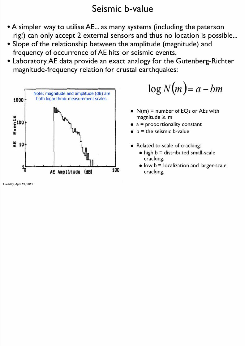
• N(m) = number of EQs or AEs withmagnitude ≥ m
• a = proportionality constant
• b = the seismic b-value
• Related to scale of cracking:
• high b = distributed small-scalecracking.
• low b = localization and larger-scale
cracking.
Note: magnitude and amplitude (dB) are
both logarithmic measurement scales.
• A simpler way to utilise AE... as many systems (including the patersonrig!) can only accept 2 external sensors and thus no location is possible...
• Slope of the relationship between the amplitude (magnitude) andfrequency of occurrence of AE hits or seismic events.
• Laboratory AE data provide an exact analogy for the Gutenberg-Richtermagnitude-frequency relation for crustal earthquakes:
Tuesday, April 19, 2011
AE during deformation of Darley Dalesandstone #1

7/31/2019 acoustic emission( )
http://slidepdf.com/reader/full/acoustic-emission- 78/82
• Sample: dry• Pc = 50 MPa
• Strain rate = 10-5 s-1
• Measurement of AE rate
and seismic b-value• AE rate increases with
crack growth up to pointof dynamic failure(past peak stress).
• b-value decreases frombackground value to aminimum around dynamicfailure.
sandstone #1
Tuesday, April 19, 2011
AE during deformation of Darley Dalesandstone #2

7/31/2019 acoustic emission( )
http://slidepdf.com/reader/full/acoustic-emission- 79/82
• Sample: water saturated
• Pc(eff) = 50 MPa
• Pf = 7 MPa (constant)
• Drained conditions
• Strain rate = 10-5 s-1
• Again, AE rate increases withcrack growth up to point of dynamic failure.
• Again, b-value decreases from
background value to aminimum around failure.
• Sample is weaker.
• More pronounced strainsoftening phase.
sandstone #2
Tuesday, April 19, 2011
AE during deformation of Darley Dalesandstone #3

7/31/2019 acoustic emission( )
http://slidepdf.com/reader/full/acoustic-emission- 80/82
• Sample: water saturated
• Initial Pc(eff) = 50 MPa
• Initial Pf = 20 MPa
• Un-drained conditions
• Strain rate = 10-5 s-1
• Pf increases during compaction,
then decreases during dilatancy.• AE increases very rapidly due to
decreasing Pc(eff).
• Cracking causes Pf to fall and Pc(eff)
to increase – so AE rate stopsaccelerating.
• Temporary strengthening duringextended strain softening phase.
• Sample fails later.
• AE shows double b-value minimumwith a recovery in between.
• This behaviour is often observed in
seismic zones prior to EQs.
sandstone #3
Tuesday, April 19, 2011

7/31/2019 acoustic emission( )
http://slidepdf.com/reader/full/acoustic-emission- 81/82

7/31/2019 acoustic emission( )
http://slidepdf.com/reader/full/acoustic-emission- 82/82
End of Lecture 2, part 3.
Even more coffee!