accuracy evaluation of nist-f1 · intai(tempsatomiqueinternational/international...

metrologia

Accuracy evaluation of NIST-F1

S. R. Jefferts, J. Shirley, T. E. Parker,T. P. Heavner, D. M. Meekhof, C. Nelson,F. Levi, G. Costanzo, A. De Marchi,R. Drullinger, L. Hollberg, W. D. Leeand F. L. Walls

Abstract. The evaluation procedure of a new laser-cooled caesium fountain primary frequency standard developedat the National Institute of Standards and Technology (NIST) is described. The new standard, NIST-F1, is describedin some detail and typical operational parameters are discussed. Systematic frequency biases for which correctionsare made – second-order Zeeman shift, black-body radiation shift, gravitational red shift and spin-exchange shift –are discussed in detail. Numerous other frequency shifts are evaluated, but are so small in this type of standard thatcorrections are not made for their effects. We also discuss comparisons of this standard both with local frequencystandards and with standards at other national laboratories.

1. Introduction

We present the evaluation procedure for NIST-F1,a laser-cooled caesium fountain primary frequencystandard operated by the NIST Time and FrequencyDivision in Boulder, Colorado, USA. NIST-F1 hasbeen operated as a frequency standard since November1998 and has undergone eleven frequency evaluations(� ve reported to the Bureau International des Poids etMesures (BIPM), six for internal use) in the intervalbetween November 1998 and August 2001. The resultsof these evaluations are shown in Section 7 (Figure 11)of this document. Five of the eleven evaluations, withType A (statistical) uncertainties less thanand Type B (systematic) uncertainties less than

have been reported to the BIPM for inclusionin TAI (Temps Atomique International/InternationalAtomic Time). The � rst two reported evaluationsused measurements of atom density and publishedcoef� cients to estimate the spin-exchange shift. Thethird and subsequent evaluations were made using arange of atom densities and extrapolating the observedfrequency to zero atom density.

S. R. Jefferts, J. Shirley, T. E. Parker, T. P. Heavner, D. M.Meekhof, C. Nelson, F. Levi,² G. Costanzo,³ A. De Marchi,³

R. Drullinger, L. Hollberg, W. D. Lee and F. L. Walls: Timeand Frequency Division, National Institute of Standards andTechnology (NIST), 325 Broadway, Boulder, CO 80303, USA.

²Permanent address: Istituto Elettrotecnico Nazionale “G. Ferraris”,Str. Delle Cacce 91, 10135 Turin, Italy.

³Permanent address: Politecnico di Torino, C.so Duca degli Abruzzi,24, 10129 Turin, Italy.

The paper is divided into seven sections. Section 2is a description of the standard. This is followedin Section 3 by a discussion of biases for whichcorrections are made. Section 4 discusses biases forwhich the standard is uncorrected. Section 5 is a briefdiscussion of the short-term stability of the standard,while Section 6 gives an overview of the evaluationprocedure. Finally, in Section 7 there is a discussion ofthe local timescale with which the standard is compared,the cumulative results and the transfer process.

2. Description of NIST-F1

2.1 Overview

NIST-F1 is designed as a primary frequency standard.Accuracy and long-term stability are the ultimate goals.Short-term stability of the reference, while importantfor operational reasons, is a secondary concern.

The fountain described here, like the LaboratoirePrimaire du Temps et des Fr Âequences (LPTF) fountain[1], uses a (0,0,1) geometry for the laser cooling andlaunching operation in which four of the six laserbeams are in the horizontal plane while two are vertical.Figure 1 illustrates the vacuum chamber and associatedstructure on NIST-F1.

The two vertical laser beams are used to launchthe atoms. A sample of about Cs atomsis � rst cooled in an optical molasses with six laserbeams at 852 nm. The sample of cold (approximately1.3 m K) atoms is launched vertically upwards fromthe optical-molasses region with an initial velocitywhich is typically about 4 m/s. The atom sample

Metrologia, 2002, 39, 321-336 321

S. R. Jefferts et al.

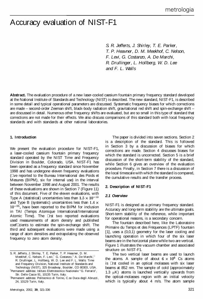
Figure 1. Mechanical drawing of the NIST-F1 physicspackage. The relevant parts of the assembly are shownalong with a scale factor.

drifts upwards through the detection region (whichis turned off when the atoms travel up) and entersthe magnetically shielded C-� eld region. The magnetic� eld (C-� eld) that provides a quantization axis in thefountain is small (in comparison with thermal beamstandards), about T ( G). After entering theC-� eld region the atoms enter the state-selection cavitywhich is used to select atoms in the “clock” state

The state selection cavity isa TE011 cavity which transfers atoms to the

state. Essentially all of the atomsremaining in the state are then removed fromthe measurement sample with an optical pulse fromthe vertical laser beams. The atoms next encounter aTE011 microwave cavity where microwave excitation isperformed. After having passed the excitation cavity onthe way up, the atoms (now in a superposition state)continue to decelerate under the in� uence of gravity.Eventually the atoms reach apogee and begin to fall.Some fraction (roughly 10 %) of the atoms (determinedprimarily by the atom temperature and toss height) re-enter the excitation cavity. The time separation betweenthe two passages through the excitation cavity hasthe same effect on the atoms as Ramsey’s (spatially)separated oscillatory-� elds method. The atoms continue

to fall, eventually leaving the C-� eld and entering thedetection region (which has been turned on by thistime) where the relative atom populations in theand hyper� ne levels are measured. The measuredpopulations of the and levels are combinedto generate an error signal used to steer the microwavefrequency synthesizer on to the frequency of the atomictransition. This constitutes one cycle of the pulsedfountain operation.

2.2 Physics package

2.2.1 Optical-molasses region

While the fountain does have a magneto-optical trap(MOT), this feature has not been used during anyof the measurements reported here. In general linear-perpendicular-linear (lin lin) molasses is used as themethod of gathering the atom sample. Table 1 givestypical parameters for the atomic source region.

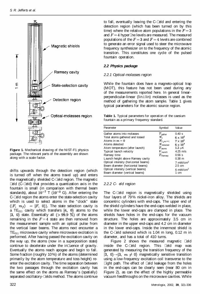
Table 1. Typical parameters for operation of the caesiumfountain as a primary frequency standard.

Parameter Symbol Value

Gather atoms into molasses gather 0.40 sTotal atoms gathered and tossedAtoms inAtoms detected detected

Atom temperature (after launch) atoms m KTypical launch velocity launch 4.25 m/sRamsey time Ramsey 0.56 sLaunch height above Ramsey cavity 0.38 mOptical intensity (horizontal beams) 7 mW/cm2

Beam diameter (horizontal beams) 2.5 cmOptical intensity (vertical beams) 6 mW/cm2

Beam diameter (vertical beams) 1 cm

2.2.2 C-� eld region

The C-� eld region is magnetically shielded usingfour layers of 79 % nickel-iron alloy. The shields areconcentric cylinders with end-caps. The upper end ofthe shield cylinders have the end-caps welded in place,while the lower end-caps are clamped in place. Theshields have holes in the end-caps for the vacuumstructure. The holes are approximately 3.5 cm indiameter in the upper end-caps and 4.2 cm in diameterin the lower end-caps. Inside the innermost shield isthe C-� eld solenoid which is 1.04 m long, 0.12 m indiameter, and has a total of 410 turns.

Figure 2 shows the measured magnetic � eldinside the C-� eld region. This � eld map wasgenerated by measuring the transition frequency of the

magnetically sensitive transitionusing a low-frequency excitation coil transverse to the� ight path. The effect of � eld leakage from the holesin the end-caps can be clearly seen (near 80 cm inFigure 2), as can the effect of the highly permeablevacuum feedthroughs on the microwave cavities. While

322 Metrologia, 2002, 39, 321-336


Figure 2. Map of the magnetic � eld in and above theRamsey cavity. The origin of the axis is the centre of theRamsey cavity. The vacuum feedthroughs on the Ramseycavity are quite permeable, and the resulting distortionsto the magnetic � eld are “corrected” by shim coils placednear the microwave cavity. This is the cause of the � elddistortions shown.

the magnetic � eld is not as homogeneous as might bedesired, the effects of the inhomogeneity are small, asdiscussed in Section 3.2.

2.2.3 Microwave cavities

The microwave cavities have been previously described[2] and only a short overview is given here. The state-selection cavity and the Ramsey cavity are identical,and the following description applies to both cavities.The cavities and the � ight tube above them servedouble duty as the vacuum wall. This design suppressesproblems with microwave leakage.

Each cylindrical cavity operates at 9.192 631 GHzin the TE011 mode and has a 3 cm radius. The cavityheight is approximately 2.18 cm. Two quarter-wavechokes suppress the unwanted TM111 mode, which isnormally degenerate with the TE011 mode. The cavityis fed magnetically in the mid-plane of the cavity byfour equally spaced circular apertures with a diameter ofapproximately 0.5 cm. The four apertures couple energyfrom a resonant mode-� lter. The cavity is severelyunder-coupled. The theoretical unloaded cavity forthis cavity is 22 000 and, as a result of the smallcoupling, the loaded is nearly equal to the unloaded

. Atoms enter and leave the cavity through long (8 cm)below-cutoff waveguides of 1 cm diameter, which arecentred on the cavity diameter. The cavity was designedwith the reduction of distributed-cavity phase shifts inmind and this system is further discussed in Section 4.

2.2.4 Detection system

The detection system consists of two regions: the � rst(upper) detects 4 atoms and the second (lower)

3 atoms. The two regions are identical with respect

to the detection systems for the atomic � uorescence,but they differ in the details of the optical interrogationbeams used.

Each � uorescence detection system uses a large(approximately 10 cm diameter) spherical mirror andan optical telescope to image the � uorescence light onto a large-area silicon photodiode. The solid angle forlight collection is (1.5 0.15) sr. The detection-systemelectrical noise is less than the signal from 10 atoms.Noise in the detection process is usually limited byscattered light from the detection beams and the overallnoise in the detected normalized signal is equivalent tothe signal from 35 atoms. The detection system appearsto reach the quantum projection noise limit at around2500 atoms. The normalization system typically lowersthe noise by less than 20 % when the fountain is workingwell. In the past we have seen much larger reductionswhen the shot-to-shot atom noise was much worse.

Detection of 4 atoms is accomplished usinga s + standing wave tuned near thecycling transition, where is the 3P3/2 state. Thestanding wave is 1 mm high by 20 mm wide (1/e2)and typically has a saturation parameter of 2.5. Directlybelow this standing wave is a travelling wave tunedto the same transition, which removes the 4 atomsso that they are not detected in the 3 detectionregion. Measurements made under operating conditionsreveal that more than 99.9 % of the (unpumped) 4atoms are removed by this beam. Some small fractionof detected 4 atoms, generally less than 3 %, arepumped into the 3 state and detected in the lowerdetection region.

3 atoms are detected using the same cyclingtransition as for the 4 atoms. The atoms are � rstoptically pumped into 4 by a standing wave tunedto the transition, and the atoms arethen detected in a standing wave similar to the onedescribed for the 4 detection system.

Both the 3 and 4 detection systems areabove the optical-molasses region. The two detectionlevels are separated by 9 cm, with the lower one about15 cm above the molasses region. Graphite in thetube between the trapping and detection regions getterscaesium from the high-pressure molasses region. Undertypical operating conditions, atoms in the 3 (lower)detection region scatter 10 % fewer photons than 4atoms as a result of the higher average vertical velocityof atoms in the lower detection level.

2.3 Optical system

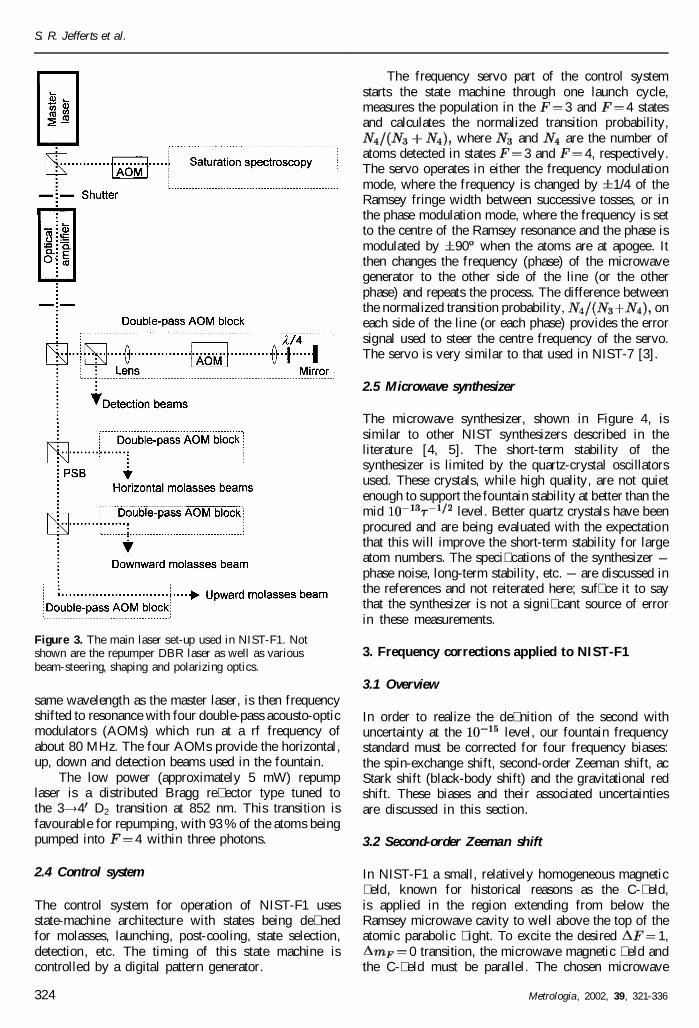
The optical system, illustrated in Figure 3, usestwo lasers and an optical ampli� er. The extended-cavity master laser injects an optical power ampli� erwhich delivers about 300 mW of optical power. Themaster laser is locked 160 MHz to the red of the4 5 D2 saturated absorption transition at 852 nm.The output of the optical power ampli� er, at the

Metrologia, 2002, 39, 321-336 323


Figure 3. The main laser set-up used in NIST-F1. Notshown are the repumper DBR laser as well as variousbeam-steering, shaping and polarizing optics.

same wavelength as the master laser, is then frequencyshifted to resonance with four double-pass acousto-opticmodulators (AOMs) which run at a rf frequency ofabout 80 MHz. The four AOMs provide the horizontal,up, down and detection beams used in the fountain.

The low power (approximately 5 mW) repumplaser is a distributed Bragg re� ector type tuned tothe 3 4 D2 transition at 852 nm. This transition isfavourable for repumping, with 93 % of the atoms beingpumped into 4 within three photons.

2.4 Control system

The control system for operation of NIST-F1 usesstate-machine architecture with states being de� nedfor molasses, launching, post-cooling, state selection,detection, etc. The timing of this state machine iscontrolled by a digital pattern generator.

The frequency servo part of the control systemstarts the state machine through one launch cycle,measures the population in the 3 and 4 statesand calculates the normalized transition probability,

where and are the number ofatoms detected in states 3 and 4, respectively.The servo operates in either the frequency modulationmode, where the frequency is changed by 1/4 of theRamsey fringe width between successive tosses, or inthe phase modulation mode, where the frequency is setto the centre of the Ramsey resonance and the phase ismodulated by 90 when the atoms are at apogee. Itthen changes the frequency (phase) of the microwavegenerator to the other side of the line (or the otherphase) and repeats the process. The difference betweenthe normalized transition probability, oneach side of the line (or each phase) provides the errorsignal used to steer the centre frequency of the servo.The servo is very similar to that used in NIST-7 [3].

2.5 Microwave synthesizer

The microwave synthesizer, shown in Figure 4, issimilar to other NIST synthesizers described in theliterature [4, 5]. The short-term stability of thesynthesizer is limited by the quartz-crystal oscillatorsused. These crystals, while high quality, are not quietenough to support the fountain stability at better than themid level. Better quartz crystals have beenprocured and are being evaluated with the expectationthat this will improve the short-term stability for largeatom numbers. The speci� cations of the synthesizerphase noise, long-term stability, etc. are discussed inthe references and not reiterated here; suf� ce it to saythat the synthesizer is not a signi� cant source of errorin these measurements.

3. Frequency corrections applied to NIST-F1

3.1 Overview

In order to realize the de� nition of the second withuncertainty at the level, our fountain frequencystandard must be corrected for four frequency biases:the spin-exchange shift, second-order Zeeman shift, acStark shift (black-body shift) and the gravitational redshift. These biases and their associated uncertaintiesare discussed in this section.

3.2 Second-order Zeeman shift

In NIST-F1 a small, relatively homogeneous magnetic� eld, known for historical reasons as the C-� eld,is applied in the region extending from below theRamsey microwave cavity to well above the top of theatomic parabolic � ight. To excite the desired 1,

0 transition, the microwave magnetic � eld andthe C-� eld must be parallel. The chosen microwave

324 Metrologia, 2002, 39, 321-336


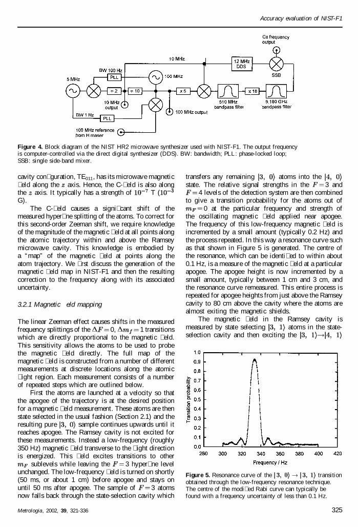
Figure 4. Block diagram of the NIST HR2 microwave synthesizer used with NIST-F1. The output frequencyis computer-controlled via the direct digital synthesizer (DDS). BW: bandwidth; PLL: phase-locked loop;SSB: single side-band mixer.

cavity con� guration, TE011, has its microwave magnetic� eld along the axis. Hence, the C-� eld is also alongthe axis. It typically has a strength of T (G).

The C-� eld causes a signi� cant shift of themeasured hyper� ne splitting of the atoms. To correct forthis second-order Zeeman shift, we require knowledgeof the magnitude of the magnetic � eld at all points alongthe atomic trajectory within and above the Ramseymicrowave cavity. This knowledge is embodied bya “map” of the magnetic � eld at points along theatom trajectory. We � rst discuss the generation of themagnetic � eld map in NIST-F1 and then the resultingcorrection to the frequency along with its associateduncertainty.

3.2.1 Magnetic � eld mapping

The linear Zeeman effect causes shifts in the measuredfrequency splittings of the 0, 1 transitionswhich are directly proportional to the magnetic � eld.This sensitivity allows the atoms to be used to probethe magnetic � eld directly. The full map of themagnetic � eld is constructed from a number of differentmeasurements at discrete locations along the atomic� ight region. Each measurement consists of a numberof repeated steps which are outlined below.

First the atoms are launched at a velocity so thatthe apogee of the trajectory is at the desired positionfor a magnetic � eld measurement. These atoms are thenstate selected in the usual fashion (Section 2.1) and theresulting pure sample continues upwards until itreaches apogee. The Ramsey cavity is not excited forthese measurements. Instead a low-frequency (roughly350 Hz) magnetic � eld transverse to the � ight directionis energized. This � eld excites transitions to other

sublevels while leaving the 3 hyper� ne levelunchanged. The low-frequency � eld is turned on shortly(50 ms, or about 1 cm) before apogee and stays onuntil 50 ms after apogee. The sample of 3 atomsnow falls back through the state-selection cavity which

transfers any remaining atoms into thestate. The relative signal strengths in the 3 and

4 levels of the detection system are then combinedto give a transition probability for the atoms out of

0 at the particular frequency and strength ofthe oscillating magnetic � eld applied near apogee.The frequency of this low-frequency magnetic � eld isincremented by a small amount (typically 0.2 Hz) andthe process repeated. In this way a resonance curve suchas that shown in Figure 5 is generated. The centre ofthe resonance, which can be identi� ed to within about0.1 Hz, is a measure of the magnetic � eld at a particularapogee. The apogee height is now incremented by asmall amount, typically between 1 cm and 3 cm, andthe resonance curve remeasured. This entire process isrepeated for apogee heights from just above the Ramseycavity to 80 cm above the cavity where the atoms arealmost exiting the magnetic shields.

The magnetic � eld in the Ramsey cavity ismeasured by state selecting atoms in the state-selection cavity and then exciting the

Figure 5. Resonance curve of the transitionobtained through the low-frequency resonance technique.The centre of the modi� ed Rabi curve can typically befound with a frequency uncertainty of less than 0.1 Hz.

Metrologia, 2002, 39, 321-336 325


magnetic-� eld-sensitive transition with a single p pulsein the Ramsey cavity. The measurement of the � eldin the Ramsey cavity typically has a 0.2 % relativeuncertainty.

The frequency data gathered using the proceduresjust described are converted into magnetic � eld unitswith the aid of published magnetic-� eld-sensitivitycoef� cients: 350.98 Hz/T for the low-frequency

3, 0, 1 transition and 700.84Hz/T for the 1, 0 transition in theRamsey cavity [6]. Higher-order terms in the magnetic-� eld sensitivity are not required at the necessary levelof precision.

In this way a magnetic-� eld map such as that shownin Figure 2 is generated. The uncertainties associatedwith each datum in Figure 2 include the positionaluncertainty at apogee (approximately 0.3 cm) and theuncertainty associated with the centre of the resonancecurve (approximately 0.1 %). These uncertainties aresmaller than the symbols used in the graph. Systematicbiases, including the Millman effect, are estimated to besmaller than the statistical uncertainties just identi� ed.

In principle, the second-order Zeeman shift of thehyper� ne transition can be directly

evaluated by calculating the time average of thesquare of the magnetic � eld, over the atomictrajectory. The published coef� cients for the second-order Zeeman effect then give a frequency shiftof d (427.45 Hz/T2) The shift isabout 400 m Hz at the C-� eld strengths typically used inNIST-F1 [6]. This method of calculating the frequencyshift directly from the measured � eld map is robust andcan be expected to have residual fractional frequencyerrors of the order of at the � eld strengthsused here. However, as a double check, we extend ourinvestigation of the magnetic � eld further, as detailedbelow.

3.2.2 Ramsey fringes, � eld maps and overlays

The Breit-Rabi formula, shown below, predicts thebehaviour of the transition frequency between theground-state hyper� ne levels with the imposition ofan external magnetic � eld. For the hyper� ne transitionsof immediate interest 1, 0) the Breit-Rabi formula can be written (up through second orderin the magnetic � eld)

(1)

where is the unshifted caesium hyper� ne transitionfrequency (in Hz), is the projection of the angularmomentum vector along the magnetic � eld (in T).The last term in (1) is the second-order Zeeman shift.

It is somewhat clearer to write the Breit-Rabi formulain terms of the dimensionless parameter as

(2)

where is Ramsey’s dimensionless � eld parameter [7]The position of the central

Ramsey fringe in the manifold can bepredicted with the use of (2) and the magnetic-� eld map.To simulate what the atoms actually experience, weaverage over the atom’s � ight time. This time averageheavily weights the region near apogee while givingless weight to the region near the cavity. For example,the 20 % of the spatial distance closest to the cavityonly contributes 11 % of the time average. Thus the� eld inhomogeneity near the cavity is relatively lessimportant at high toss heights.

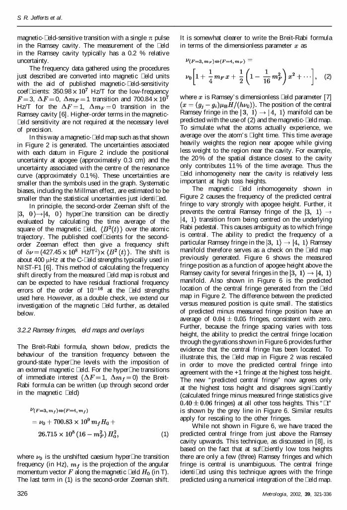
The magnetic � eld inhomogeneity shown inFigure 2 causes the frequency of the predicted centralfringe to vary strongly with apogee height. Further, itprevents the central Ramsey fringe of the

transition from being centred on the underlyingRabi pedestal. This causes ambiguity as to which fringeis central. The ability to predict the frequency of aparticular Ramsey fringe in the Ramseymanifold therefore serves as a check on the � eld mappreviously generated. Figure 6 shows the measuredfringe position as a function of apogee height above theRamsey cavity for several fringes in themanifold. Also shown in Figure 6 is the predictedlocation of the central fringe generated from the � eldmap in Figure 2. The difference between the predictedversus measured position is quite small. The statisticsof predicted minus measured fringe position have anaverage of fringes, consistent with zero.Further, because the fringe spacing varies with tossheight, the ability to predict the central fringe locationthrough the gyrations shown in Figure 6 provides furtherevidence that the central fringe has been located. Toillustrate this, the � eld map in Figure 2 was rescaledin order to move the predicted central fringe intoagreement with the +1 fringe at the highest toss height.The new “predicted central fringe” now agrees onlyat the highest toss height and disagrees signi� cantly(calculated fringe minus measured fringe statistics give

fringes) at all other toss heights. This “� t”is shown by the grey line in Figure 6. Similar resultsapply for rescaling to the other fringes.

While not shown in Figure 6, we have traced thepredicted central fringe from just above the Ramseycavity upwards. This technique, as discussed in [8], isbased on the fact that at suf� ciently low toss heightsthere are only a few (three) Ramsey fringes and whichfringe is central is unambiguous. The central fringeidenti� ed using this technique agrees with the fringepredicted using a numerical integration of the � eld map.

326 Metrologia, 2002, 39, 321-336


Figure 6. The various symbols connected by dashed linesare the position of Ramsey fringes from the hyper� nemanifold as a function of distance above the Ramsey cavity.The solid black line represents the predicted position ofthe central fringe from the time integral of the magnetic� eld in Figure 2 for apogee at various heights above theRamsey cavity. The agreement between the predicted andmeasured fringe is quite good, with an average discrepancyof fringes. The grey line results from rescalingthe � eld map in Figure 2 to get agreement with an adjacentfringe. This is not successful, with the predicted fringemissing the measured fringe by an average offringes. See Section 3.2 for a complete discussion.

In NIST-F1 the numerical integration is considerablyless time-consuming than laboriously following thecentral fringe from an apogee 0.5 cm above the Ramseycavity to a � nal apogee at 50 cm or more.

While there is no reason to believe that the centralfringe has been misidenti� ed, we assign a (perhapsoverly) conservative error of d in theuncertainty budget shown in Table 2. The fractionaluncertainty assigned is equivalent to one full fringe atthe � eld values used in NIST-F1.

Once the central fringe on themanifold has been identi� ed it can be used to predict thefrequency offset of the transition due tomagnetic � eld. Let be the frequency differencebetween the andtransitions. Then, from (2), the frequency correctiondue to the magnetic � eld (second-order Zeeman shift)on the transition can be written

(3)

There are several reasons for using this method tocorrect for the second-order Zeeman shift. First, theuse of (3) suppresses a small bias due to underlyingpedestal shifts as discussed in [3]. Second, the frequencyof the central fringe can be monitored to observe(and if necessary correct for) time � uctuations of themagnetic � eld. The magnetic � eld in NIST-F1 has been

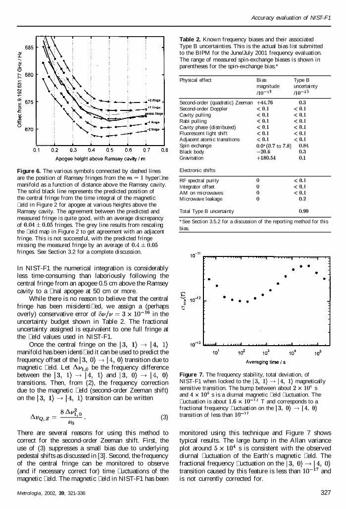
Table 2. Known frequency biases and their associatedType B uncertainties. This is the actual bias list submittedto the BIPM for the June/July 2001 frequency evaluation.The range of measured spin-exchange biases is shown inparentheses for the spin-exchange bias.*

Physical effect Bias Type Bmagnitude uncertainty/ / 5

Second-order (quadratic) ZeemanSecond-order DopplerCavity pullingRabi pullingCavity phase (distributed)Fluorescent light shiftAdjacent atomic transitionsSpin exchange * toBlack bodyGravitation

Electronic shifts

RF spectral purityIntegrator offsetAM on microwavesMicrowave leakage

Total Type B uncertainty

*See Section 3.5.2 for a discussion of the reporting method for thisbias.

Figure 7. The frequency stability, total deviation, ofNIST-F1 when locked to the magneticallysensitive transition. The bump between about sand 4 s is a diurnal magnetic � eld � uctuation. The� uctuation is about T and corresponds to afractional frequency � uctuation on thetransition of less than

monitored using this technique and Figure 7 showstypical results. The large bump in the Allan varianceplot around s is consistent with the observeddiurnal � uctuation of the Earth’s magnetic � eld. Thefractional frequency � uctuation on thetransition caused by this feature is less than andis not currently corrected for.

Metrologia, 2002, 39, 321-336 327


A possible frequency bias results from the magnetic� eld inhomogeneity and the use of (3). The frequencyoffset is, in essence, a measure of the timeaverage of the magnetic � eld as seen by the atoms,

This average is then squared with the use of(3) and the squared average, is used in placeof This type of error is discussed more fullyin [3]. In NIST-F1 the fractional frequency bias fromthis effect is less than and is not corrected for.

3.3 Black-body radiation frequency shift

The ac Stark shift from the thermal radiationenvironment of the atoms, � rst calculated by Itano etal. [9], has recently been measured by two separategroups [10, 11]. The experimental results combinedwith theoretical results give a frequency shift of

d

(4)

where is the temperature (in kelvins) of a perfectblack body producing the radiation. The atomic-� ightregion of NIST-F1 is temperature controlled at about41 C. There is a small temperature gradient betweenthe Ramsey cavity and atom apogee of less than 0.5 C.The � ight path of the atoms is well shielded fromthe outside world and the thermal radiation insidethe standard should therefore be representative of thetemperature measured by the thermocouples attached tothe � ight tube. The average wall temperature seen by theatoms is only very slightly shifted by the temperaturegradient because the atoms spend the vast majorityof the time in the apparatus near apogee where thetemperature is essentially constant. With these data inhand the black-body radiation shift can be calculatedto be d with an uncertainty of

corresponding to a 1 C uncertainty in theradiation temperature.

The temperature of the radiation � eld inside thedrift tube is somewhat uncertain, but the opticallycoated window at the top of the drift tube is within 5 Cof the drift-tube temperature and should be relatively“black” in the infrared. Furthermore the solid anglesubtended by this window is small ( sr) as“seen” by the atom ball. The radiation � eld sampled bythe atoms should thus be well characterized by the walltemperature. The room is kept dark when the standardis being operated.

3.4 Gravitational frequency shift

The altitude in Boulder, CO, where NIST-F1 is located,is about 1600 m. General relativistic calculations predicta fractional increase in the frequency of a clock whenoperated above the rotating geoid of m .

In order for NIST-F1 to be compared with andcontribute to TAI the clock frequency must be correctedto the geoid. The clock frequency reported therefore hasa fractional frequency correction of withan uncertainty of [12].

3.5 Spin-exchange frequency shift

The spin-exchange shift in a caesium fountain isextraordinarily large [13, 14] as well as being energydependent [15] and must be corrected to enable caesiumfountains to produce accuracies of better than a fewparts in . The spin-exchange coef� cient has beenmeasured by several groups [13, 14]. The currentunderstanding that the spin-exchange shift is energydependent makes the measurements reported in [13, 14]somewhat uncertain. As a result of this uncertainty, wehave switched from a method which used the spin-exchange coef� cient as reported in [13, 14] alongwith an absolute density determination (used in the� rst two formal accuracy evaluations) to a densityextrapolation method described next. It is importantto note that, within the stated uncertainties of the twomethods, the results of the spin-exchange correctionusing the previously reported spin-exchange coef� cientand absolute density determination are in agreementwith the results obtained by extrapolation to zerodensity.

3.5.1 Extrapolation to zero density

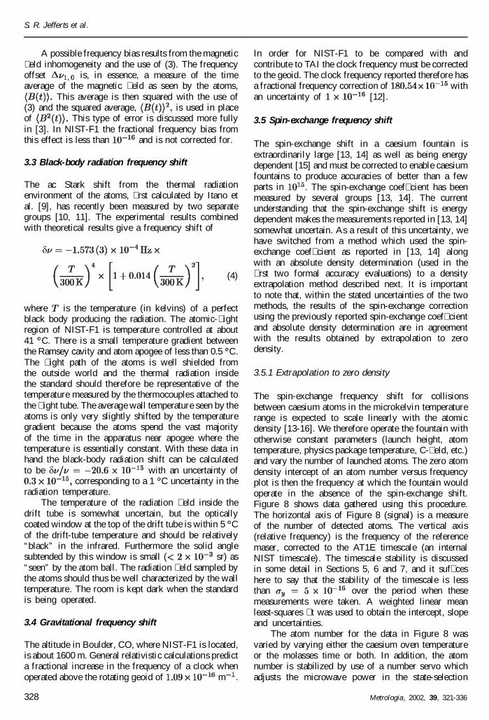
The spin-exchange frequency shift for collisionsbetween caesium atoms in the microkelvin temperaturerange is expected to scale linearly with the atomicdensity [13-16]. We therefore operate the fountain withotherwise constant parameters (launch height, atomtemperature, physics package temperature, C-� eld, etc.)and vary the number of launched atoms. The zero atomdensity intercept of an atom number versus frequencyplot is then the frequency at which the fountain wouldoperate in the absence of the spin-exchange shift.Figure 8 shows data gathered using this procedure.The horizontal axis of Figure 8 (signal) is a measureof the number of detected atoms. The vertical axis(relative frequency) is the frequency of the referencemaser, corrected to the AT1E timescale (an internalNIST timescale). The timescale stability is discussedin some detail in Sections 5, 6 and 7, and it suf� ceshere to say that the stability of the timescale is lessthan over the period when thesemeasurements were taken. A weighted linear meanleast-squares � t was used to obtain the intercept, slopeand uncertainties.

The atom number for the data in Figure 8 wasvaried by varying either the caesium oven temperatureor the molasses time or both. In addition, the atomnumber is stabilized by use of a number servo whichadjusts the microwave power in the state-selection

328 Metrologia, 2002, 39, 321-336


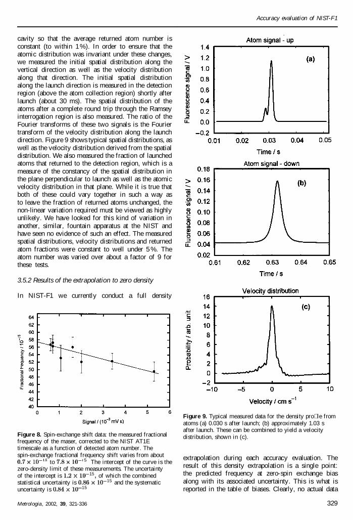
cavity so that the average returned atom number isconstant (to within 1 %). In order to ensure that theatomic distribution was invariant under these changes,we measured the initial spatial distribution along thevertical direction as well as the velocity distributionalong that direction. The initial spatial distributionalong the launch direction is measured in the detectionregion (above the atom collection region) shortly afterlaunch (about 30 ms). The spatial distribution of theatoms after a complete round trip through the Ramseyinterrogation region is also measured. The ratio of theFourier transforms of these two signals is the Fouriertransform of the velocity distribution along the launchdirection. Figure 9 shows typical spatial distributions, aswell as the velocity distribution derived from the spatialdistribution. We also measured the fraction of launchedatoms that returned to the detection region, which is ameasure of the constancy of the spatial distribution inthe plane perpendicular to launch as well as the atomicvelocity distribution in that plane. While it is true thatboth of these could vary together in such a way asto leave the fraction of returned atoms unchanged, thenon-linear variation required must be viewed as highlyunlikely. We have looked for this kind of variation inanother, similar, fountain apparatus at the NIST andhave seen no evidence of such an effect. The measuredspatial distributions, velocity distributions and returnedatom fractions were constant to well under 5 %. Theatom number was varied over about a factor of 9 forthese tests.

3.5.2 Results of the extrapolation to zero density

In NIST-F1 we currently conduct a full density

Figure 8. Spin-exchange shift data: the measured fractionalfrequency of the maser, corrected to the NIST AT1Etimescale as a function of detected atom number. Thespin-exchange fractional frequency shift varies from about

to 5 The intercept of the curve is thezero-density limit of these measurements. The uncertaintyof the intercept is 15 of which the combinedstatistical uncertainty is 15 and the systematicuncertainty is 15

Figure 9. Typical measured data for the density pro� le fromatoms (a) 0.030 s after launch; (b) approximately 1.03 safter launch. These can be combined to yield a velocitydistribution, shown in (c).

extrapolation during each accuracy evaluation. Theresult of this density extrapolation is a single point:the predicted frequency at zero-spin exchange biasalong with its associated uncertainty. This is what isreported in the table of biases. Clearly, no actual data

Metrologia, 2002, 39, 321-336 329


are gathered at zero density. Because the density isvaried over almost an order of magnitude, no uniquespin-exchange bias can be reported in Table 2.

Other fountain groups typically measure the slopeof the extrapolation curve one or more times and usethis historical slope to correct data with a “known”spin-exchange shift. The bias in the latter case wouldnot be zero.

The majority of time gathering the data in Figure 8is spent on the low atomic density data, which have aspin-exchange shift of less than d Theuncertainty of the intercept for the data in Figure 8 isd which we regard as a combinationof both systematic and statistical uncertainties. Weseparate these as follows. The intercept uncertainty isregarded as the quadrature sum of the total statisticaluncertainty of the points in Figure 8 and an unknownsystematic shift; the unknown systematic uncertaintyis then the square root of the difference betweenthe square of the uncertainty in the intercept and thesquare of the statistical uncertainty of the data set. Thisprocedure yields a fractional systematic uncertainty inthe spin-exchange shift of for the data inFigure 8. The separation of the data in this fashionhas the advantage that when the BIPM recombines theType A and Type B uncertainties the combined standarduncertainty, which is the quadrature sum of the Type Aand Type B uncertainties, is correct. The choice is,however, arbitrary and in fact the combined standarduncertainty is the important number.

3.5.3 Other techniques, MOTs vs molasses

We have used only optical molasses in these tests.The use of density extrapolation with a MOT-basedsource requires, in the light of the present understandingthat the spin-exchange coef� cient is highly energydependent [15], a great deal of caution. The diameterof the atomic sample when using a MOT is knownto grow with the atom number. The collision energychanges over timescales on the order of the diameterof the initial sample size divided by the “thermal”velocity. With typical MOT sizes of a few millimetresand velocities of about 1 cm/s, this results in theaverage collision energy being a strong function ofthe atomic number when using a MOT. As a resultof these considerations we use exclusively a molasseswhich does not suffer from this defect. Note that itshould be possible to use a number servo such asthat described in Section 3.5.1, with a MOT in whichthe parameters are held constant and the atom numbervaried by state-selection power to keep the averagecollision energy more nearly constant. Even in the caseof a “constant” MOT, however, small misalignmentsof the beams can lead to varying spatial distributions(as a result of imparted angular momentum) withoutundue effect on the launched number. This leads to avarying average collision energy with time and thus

non-constant spin-exchange shift. The effect is likely tobe much more pronounced in the case of a MOT thanwith optical molasses.

4. Frequency biases not corrected in NIST-F1and their associated magnitudes

4.1 Overview

A large number of biases that are of concern in atraditional thermal-beam caesium frequency standardare considerably reduced in the fountain as a resultof the long Ramsey time. Additionally, other possiblebiases such as electronically caused shifts have beenevaluated and an upper limit set on them. These biases,all of which turn out to be either intrinsically smallor are kept small through experimental practice, arediscussed in this section.

4.2 Doppler shifts of � rst and second order

The � rst-order Doppler shift, which manifests itselfprimarily as distributed-cavity phase shift, is causedby atoms sampling different phases of the microwave� eld within the Ramsey cavity during their two tripsthrough the cavity. In the best of all possible worlds,this phase shift would be absent as the phase of themicrowave � elds within the cavity would be constant.The cavities used in NIST-F1 are designed to havea small distributed phase, thereby minimizing theassociated frequency shift [2]. The calculated phaseextrema for the cavity are of magnitude m rad at theedge of the aperture through which atoms travel. As a(physically unrealizable) worst-case scenario, considerthat all the atoms in the atom ball sample a phase of

m rad on the way up through the Ramsey cavityand sample a phase of m rad on the way down.This would cause a fractional frequency shift of order

and is neglected here.The possibility of a longitudinal phase gradient

also exists. In the fountain geometry, time-reversalsymmetry causes this effect to be largely cancelled.The residual (uncancelled) portion of the longitudinalphase gradient is proportional (to � rst order) to thetransverse phase along the atomic trajectory divided bythe square of the cavity half-height. The phase of themicrowave � eld at the aperture is essentially constantwhile the phase at the centre of the cavity is morecomplex, as described in [2]. The number of cavityfeeds is also critical in the longitudinal phase in afountain, because a frequency shift enters as a resultof the differential longitudinal phase gradient acrossthe cavity aperture rather than the longitudinal phasegradient. The cavity used in NIST-F1 is almost twoorders of magnitude less sensitive to this effect than thecavity described in [17]. The relative frequency shiftresulting from residual longitudinal phase gradients inNIST-F1 is less than

330 Metrologia, 2002, 39, 321-336


The second-order Doppler effect is relativistic innature: moving clocks run slow. An advantage ofthe fountain over traditional beam standards is thatthe atoms in a fountain standard move very slowly.The second-order Doppler effect for atoms with a1 s Ramsey time is of order and is notcorrected for, although it could easily be corrected forif necessary.

4.3 Rabi and Ramsey pulling

Rabi pulling, caused by tails of excitation of others transitions in the microwave transitionspectrum, is almost absent in this standard as a resultof state selection. As a worst-case estimate, consideran excitation of only the s transition with aheight 10 % of the central peak (note that this has neverbeen observed in our clock; typically the and

Rabi peaks have less than 0.1 % the heightof the clock transition Rabi peak). For this worst-caseestimate, the fractional frequency shift as a result ofRabi pulling is about Using the experimentaldata measured after state selection, the calculated Rabipulling is of order This shift is not corrected for.

Ramsey pulling is caused by excitation of thep transition as well

as the although the latter transition isnot favoured in our state-selected standard. This typeof transition is excited if the microwave magnetic � eldand the C-� eld are not exactly parallel at all locationswhere atoms sample the microwave � eld. This lack ofparallelism is guaranteed to occur within our microwavecavity with its half-sine-wave intensity pro� le. Ramseypulling is extremely dif� cult to evaluate completely andwe give only a � rst-order glance at the problem here.Possible coherence effects in the atomic sample havenot been evaluated; however, the state-selection processwith an optical pulse to remove atoms shoulddestroy any coherence by projecting the remainingatoms into the state. More complete results willbe published elsewhere.

Cutler et al. have given a simpli� ed theory thatprovides an order of magnitude estimate of the problem[18]. Ramsey pulling is proportional to the differencebetween the population of the atoms making the

transition and the population making thetransition, relative to the population making

the clock transition. In NIST-F1 less than 0.1 % of theatoms make a transition and the left/rightasymmetry is less than 10 %. Given the T C-� eld,the approximate order of magnitude of the fractionalfrequency shift due to the Ramsey pulling terms in [6]is and is not corrected for.

4.4 Majorana transitions

This fountain is state selected within the magneticshields. The detection system is essentially insensitive

to the state of the arriving caesium population, beingsensitive only to the state. Therefore, Majoranatransitions can cause a frequency shift only if suchtransitions take place within the magnetic shieldstructure. Majorana transitions occur if the so-calledadiabatic condition is not ful� lled [6]. The adiabaticcondition can be written

p(5)

where describes the � eld variation, is the anglebetween (the magnetic � eld vector) andis the length scale of the � eld variation, and isthe velocity of the atoms through the � eld variation.This condition is satis� ed in NIST-F1 by more thanthree orders of magnitude. The probability is thatnot a single atom in the caesium cloud makes aMajorana transition within the magnetically shieldedregion. Given the measured populations in ofless than (limited by S/N) relative to thepopulation after state selection and assuming a 100 %left/right asymmetry yields a potential frequency shiftof d [19]. Additionally, as explained in[19], proper choice of the C-� eld value suppresses thisshift further. The C-� eld value in NIST-F1 is carefullychosen to satisfy the conditions for suppression offrequency shifts due to Majorana transitions so thatthe potential d is suppressed furtherby more than an order of magnitude. This possiblefrequency shift is not corrected for. Zeeman coherencesinduced by the magnetic � eld inhomogeneity should notin principle cause a frequency shift. However, as a testwe applied a 100 ms pulse of resonant low-frequencyexcitation to the sample about apogee (as described inSection 3.2) during an otherwise normal measurementof the fountain frequency. No frequency shift wasmeasured with a resolution of d eventhough the applied pulse was suf� cient to induce a 25 %coherence and is more than times more likely toinduce coherence than the magnetic � eld inhomogeneityshown in Figure 2.

4.5 Spectral impurities and microwave leakage

The microwave spectrum has been measured and fromthese measurements a worst-case frequency offset of

is predicted. As an additional operationaltest, the fountain is operated in a range of microwavepowers above optimal: as much as 120 times optimalpower (11 p pulses rather than p No microwave-power-dependent frequency shift has been measured atany elevated microwave power level. Assuming thatwe are well below saturation in any power-dependenteffect, any shift should be linear in the microwave� eld. Although the resolution of the measurement islimited by the measurement times used, this still placesa limit on the effects of spectral impurities of about

under the assumption of linearity of theshift with � eld. In particular, we have never observed

Metrologia, 2002, 39, 321-336 331


a power-dependent frequency shift such as reported inthe LPTF fountain, in spite of repeated attempts to doso [20].

The design of NIST-F1 is intrinsically well shieldedfrom microwave leakage. However, the high-powertest just described also tests for a possible microwaveleakage error. Frequency shifts as a result of microwaveleakage in the fountain geometry are also mainlycancelled as a result of the time-reversal symmetryof the atomic � ight through the Ramsey interaction.

4.6 DC Stark effect

The entire microwave interaction region and the drifttube above it are constructed from oxygen-free high-purity copper. Further, temperature gradients along thisstructure are minimized by active control. The structureis allowed an electrical connection to the outside worldat only one place. In view of all these precautions,it is unreasonable to expect a potential difference ofeven a volt over the length of the standard. Assuminga potential as large as 1 V, the associated electric� eld would be of order 1 V/m, leading to a fractionalfrequency shift of less than As a worst case,we can assume a 1 V patch � eld inside the cutoffdrift tube; this could provide electric � eld strengths oforder 100 V/m, leading to a frequency shift of around

(the atoms spend a small fraction of the timein this region). A 1 V patch � eld in the drift tube at theapogee of the atomic � ight would lead to a frequencyshift of less than No corrections are made forthe dc Stark effect.

4.7 Cavity pulling

Cavity pulling effects are quite small in this standardin spite of the high cavity The cavityis essentially unloaded and the resulting cavity isessentially the theoretical cavity for the size ofcavity and material (oxygen-free copper). For smallcavity detunings, the second-order cavity pulling effectcan be written

d

p

d(6)

where is the atomic line p and d isthe cavity detuning [6]. Assuming that the microwavepower is within 1 dB of optimum and that the cavity iskept within one cavity linewidth of the transition, thepulling is only about In actual operation thecavity is tuned to within much less than one linewidthand the microwave power is closer than 1 dB tooptimum. We project a worst-case cavity pulling of

This shift is presently uncorrected for.First-order cavity pulling, as reported in [21], is

much less than d over the range of atomicdensities used in NIST-F1.

4.8 Resonant light shift

The laser system for NIST-F1 has three mechanicalshutters used to prevent unwanted resonant light fromreaching the atoms: one on the DBR repumper section,one between the extended cavity master laser and theoptical ampli� er, and one on the output of the opticalampli� er. Additionally, the AOMs are shut off whenthe atoms are within the C-� eld region.

To test the effectiveness of the shuttering, theshutter between the master laser and the opticalampli� er was removed. In this case the ampli� erdelivers approximately 30 dB more optical power thanwhen uninjected. In this con� guration, 30 dB moreresonant light is produced, yet no resonant light shiftgreater than has been observed. We thereforeestimate that the resonant light shift when running inthe normal con� guration (three shutters) should be lessthan

The standard is routinely surveyed with an infraredscanner in order to identify scattered light paths thatenter the fountain structure. The room lights areextinguished when the standard is being operated andparts of the standard are draped with an opaque clothcover.

4.9 Servo biases

The servo system used in NIST-F1 is closely related tothe NIST-7 servo system described in [3]. The linewidthsplitting required in NIST-7 is, as a consequence of its72 Hz Ramsey fringe width and accuracy,considerably more challenging than the fringe splittingrequired for NIST-F1, with its 1 Hz Ramsey fringe and

accuracy.Two classes of error could be associated with the

servo. First is a sloping baseline under the Ramseyfringe. The analysis for this type of error is similar to theanalysis required for cavity-pulling effects; for afrequency bias an effective of located halfof the “resonance” linewidth from the central Ramseyfringe would be required. No such effect has beenobserved. This effect can also be tested by lockingthe standard on fringes well removed from the centralfringe. For example, we have operated the fountainby measuring the left side of the 10th fringe andthe right side of the 10th fringe. This causes theeffective fringe width to be greatly increased, therebyenhancing the effect of a sloping baseline. No frequencyoffset is observed under these conditions with sensitivityto a frequency shift on the central fringe.Additionally, phase modulation, which we often use onour fountain, is much less sensitive to this effect thanfrequency modulation.

The second class of potential servo offsets comesfrom a possible synthesizer frequency offset. We havecompared our frequency synthesizer with a newerdesign, discussed in [5]. The comparison showed no

332 Metrologia, 2002, 39, 321-336


frequency offset at the level, even thoughthe synthesizers operate using completely differenttopologies and components.

4.10 Background gas collisions

Measured pressure in NIST-F1, along with knownconductivities, pressure shift coef� cients and residualgas analysis, leads to the estimate of fractionalfrequency shift from this effect of less than[22]. Given the uncertainty of this estimate, however,we assign a somewhat larger systematic uncertainty ofd

5. Frequency stability

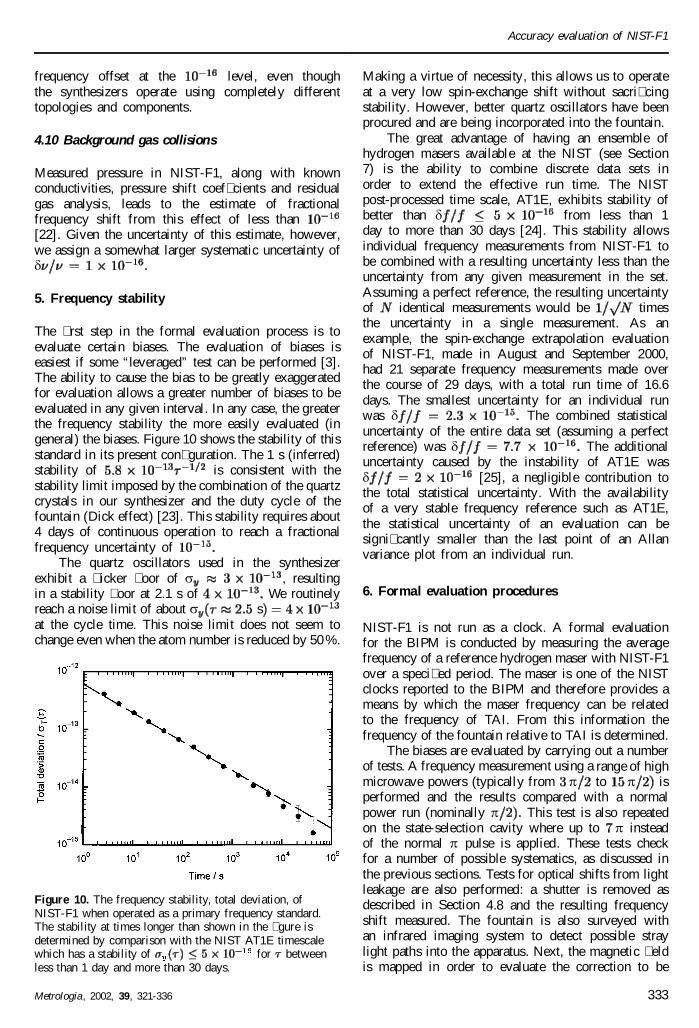
The � rst step in the formal evaluation process is toevaluate certain biases. The evaluation of biases iseasiest if some “leveraged” test can be performed [3].The ability to cause the bias to be greatly exaggeratedfor evaluation allows a greater number of biases to beevaluated in any given interval. In any case, the greaterthe frequency stability the more easily evaluated (ingeneral) the biases. Figure 10 shows the stability of thisstandard in its present con� guration. The 1 s (inferred)stability of is consistent with thestability limit imposed by the combination of the quartzcrystals in our synthesizer and the duty cycle of thefountain (Dick effect) [23]. This stability requires about4 days of continuous operation to reach a fractionalfrequency uncertainty of

The quartz oscillators used in the synthesizerexhibit a � icker � oor of s , resultingin a stability � oor at 2.1 s of We routinelyreach a noise limit of about s sat the cycle time. This noise limit does not seem tochange even when the atom number is reduced by 50 %.

Figure 10. The frequency stability, total deviation, ofNIST-F1 when operated as a primary frequency standard.The stability at times longer than shown in the � gure isdetermined by comparison with the NIST AT1E timescalewhich has a stability of for betweenless than 1 day and more than 30 days.

Making a virtue of necessity, this allows us to operateat a very low spin-exchange shift without sacri� cingstability. However, better quartz oscillators have beenprocured and are being incorporated into the fountain.

The great advantage of having an ensemble ofhydrogen masers available at the NIST (see Section7) is the ability to combine discrete data sets inorder to extend the effective run time. The NISTpost-processed time scale, AT1E, exhibits stability ofbetter than d from less than 1day to more than 30 days [24]. This stability allowsindividual frequency measurements from NIST-F1 tobe combined with a resulting uncertainty less than theuncertainty from any given measurement in the set.Assuming a perfect reference, the resulting uncertaintyof identical measurements would be timesthe uncertainty in a single measurement. As anexample, the spin-exchange extrapolation evaluationof NIST-F1, made in August and September 2000,had 21 separate frequency measurements made overthe course of 29 days, with a total run time of 16.6days. The smallest uncertainty for an individual runwas d The combined statisticaluncertainty of the entire data set (assuming a perfectreference) was d The additionaluncertainty caused by the instability of AT1E wasd [25], a negligible contribution tothe total statistical uncertainty. With the availabilityof a very stable frequency reference such as AT1E,the statistical uncertainty of an evaluation can besigni� cantly smaller than the last point of an Allanvariance plot from an individual run.

6. Formal evaluation procedures

NIST-F1 is not run as a clock. A formal evaluationfor the BIPM is conducted by measuring the averagefrequency of a reference hydrogen maser with NIST-F1over a speci� ed period. The maser is one of the NISTclocks reported to the BIPM and therefore provides ameans by which the maser frequency can be relatedto the frequency of TAI. From this information thefrequency of the fountain relative to TAI is determined.

The biases are evaluated by carrying out a numberof tests. A frequency measurement using a range of highmicrowave powers (typically from p to p isperformed and the results compared with a normalpower run (nominally p This test is also repeatedon the state-selection cavity where up to p insteadof the normal p pulse is applied. These tests checkfor a number of possible systematics, as discussed inthe previous sections. Tests for optical shifts from lightleakage are also performed: a shutter is removed asdescribed in Section 4.8 and the resulting frequencyshift measured. The fountain is also surveyed withan infrared imaging system to detect possible straylight paths into the apparatus. Next, the magnetic � eldis mapped in order to evaluate the correction to be

Metrologia, 2002, 39, 321-336 333


applied for the quadratic Zeeman shift. The atomicspatial distribution and temperature as a function ofatom number are checked for constancy over a rangeof molasses load time and Cs oven temperatures. Thisallows extrapolation of the spin-exchange frequencyshift as a function of the number of Cs atoms.

The standard is then run to measure the frequencyof the reference maser, which is in turn referenced tothe AT1E timescale. This process may take severaldays, as the fountain is operated long enough tobring the statistical uncertainty down to an acceptablelevel. The atomic density is then varied and the abovemeasurement repeated in order to construct a plot ofatom number versus measured frequency. These dataare eventually used to determine the frequency of themaser corrected for the spin-exchange shift. Becauseof the high stability of the timescale s 1 day

30 days the fountain does notneed to run continuously during this period. The mostimportant parameter is total accumulated run time.A signi� cant amount of dead time can be toleratedwithout seriously affecting the overall uncertainty ofthe evaluation [25, 26]. During the course of thefrequency measurement, the environmental parametersof all � ve reference masers (temperature, relativehumidity, vertical magnetic � eld, barometric pressureand power line voltage) are monitored along with theirfrequency stability (see Section 7).

If any signi� cant change is seen in operationalparameters of the fountain over the course of themeasurement, some or all of the bias evaluations arerepeated. Most of the tests described in Sections 3and 4 are repeated routinely and can be consideredpart of a formal evaluation. The � nal step is to applythe measured bias corrections as listed in Table 2and report the corrected frequency to the BIPM.The biases and uncertainties in Table 2 are thosereported to the BIPM for the � fth formal evaluation ofNIST-F1. The statistical uncertainty for this evaluationwas giving a combined uncertainty of

It should be realized that Table 2 lists allknown biases for NIST-F1; unknown biases cannot, byde� nition, be corrected.

7. Performance assessment

7.1 Introduction

In addition to the careful evaluation of all biases, asdescribed above, it is also useful to assess the long-term (run-to-run) stability of the standard. This can beaccomplished if a suf� ciently stable frequency referenceis available. A clear indication is given that somethingis not under control if the long-term frequency stabilityof a standard is not consistent with the combineduncertainty of the standard and the stability of thereference. Frequency comparisons against other primaryfrequency standards should also be made.

7.2 Internal comparisons

The NIST is fortunate to have an ensemble of � veactive, cavity-tuned hydrogen masers and four high-performance commercial caesium-beam tube standards.This ensemble [27, 28], is used to produce a post-processed scale, AT1E [24], that exhibits a frequencystability of at 10 days and which isbetter than over the range 0.2 to 100 days.The frequency drift rate of AT1E is of the order of

per year.A frequency reference with this high stability

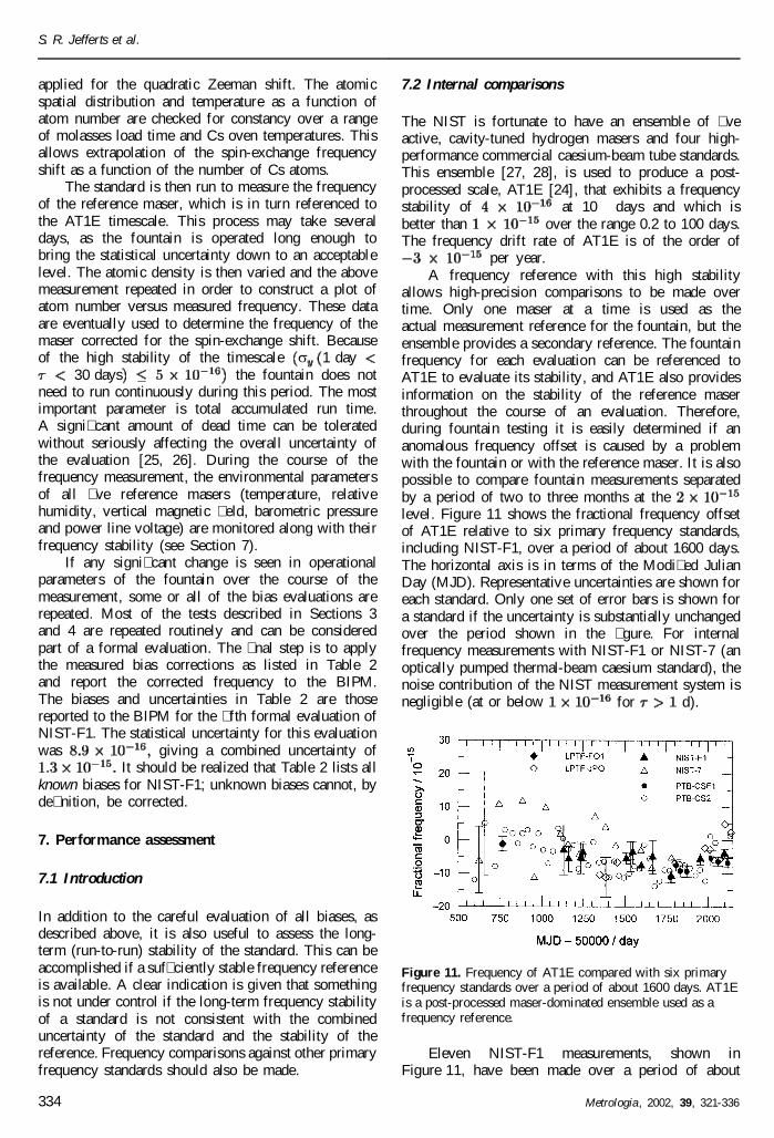
allows high-precision comparisons to be made overtime. Only one maser at a time is used as theactual measurement reference for the fountain, but theensemble provides a secondary reference. The fountainfrequency for each evaluation can be referenced toAT1E to evaluate its stability, and AT1E also providesinformation on the stability of the reference maserthroughout the course of an evaluation. Therefore,during fountain testing it is easily determined if ananomalous frequency offset is caused by a problemwith the fountain or with the reference maser. It is alsopossible to compare fountain measurements separatedby a period of two to three months at thelevel. Figure 11 shows the fractional frequency offsetof AT1E relative to six primary frequency standards,including NIST-F1, over a period of about 1600 days.The horizontal axis is in terms of the Modi� ed JulianDay (MJD). Representative uncertainties are shown foreach standard. Only one set of error bars is shown fora standard if the uncertainty is substantially unchangedover the period shown in the � gure. For internalfrequency measurements with NIST-F1 or NIST-7 (anoptically pumped thermal-beam caesium standard), thenoise contribution of the NIST measurement system isnegligible (at or below for d).

Figure 11. Frequency of AT1E compared with six primaryfrequency standards over a period of about 1600 days. AT1Eis a post-processed maser-dominated ensemble used as afrequency reference.

Eleven NIST-F1 measurements, shown inFigure 11, have been made over a period of about

334 Metrologia, 2002, 39, 321-336


1000 days and all are statistically consistent withintheir individual uncertainties and the stability of AT1E.Two different reference masers were used for thesemeasurements. Note that the fountain uncertaintieshave generally decreased with time as the performanceof the fountain has improved. The � fth measurement,made over a period of 4.1 days centred on MJD 51508(26 November 1999), was the � rst formal evaluation ofNIST-F1, and the result was reported to the BIPM. Theseventh, ninth, tenth and eleventh data points were alsoformal evaluations that were reported to the BIPM.All other data points were informal evaluations and, inmost of these cases, the runs were short. This resultedin relatively large statistical uncertainties.

The availability of a stable reference increasescon� dence in the stated uncertainties when themeasurements made over a period of time areconsistent. This self-consistency is a necessary, but notsuf� cient, condition for having correctly determinedthe overall uncertainty of the standard. Ten NIST-7evaluations were performed during the period ofoperation of the fountain and these evaluations are alsoconsistent with the fountain measurements within thestated uncertainties of NIST-7.

7.3 External comparisons

Figure 11 also shows data for the Physikalisch-Technische Bundesanstalt (PTB) thermal-beam caesiumstandard CS2 and the new PTB fountain standardCSF1 [8]. Two LPTF standards, LPTF-FO1 (a caesiumfountain) and LPTF-JPO (an optically pumped thermal-beam standard) are also shown. The data for thesestandards were taken from Circular T and the AnnualReport of the Time Section of the BIPM, or wereobtained through direct communications with the staffat the PTB. Long-distance comparisons are all degradedto some extent by instabilities in the time-transfertechnique. Most of the data are for 30-day evaluationintervals using common-view GPS, which gives a timetransfer uncertainty of about at 30 days.However, the seven comparisons with PTB-CSF1 werefor 15-day (or in the last case 20-day) intervals andwere made using two-way time transfer. The two-waylink with the PTB has demonstrated greater stabilitythan common-view GPS and gives a time transferuncertainty of for a 15-day interval [29].The total uncertainties represented by the error bars forthe PTB and LPTF standards include the time-transferuncertainty. The comparisons with the remote standardscould also have been made using TAI as the reference.

As may be seen in Figure 11, the NIST-F1 measurements are in agreement within stateduncertainties with other standards that were operatedat the same, or nearly the same, time. The sevenPTB-CSF1 measurements are particularly important, asthey were made over the same period as the last threeNIST-F1 measurements and the agreement is good. The

approximately 400-day period between the last reportedLPTF fountain measurement and the earliest NIST-F1evaluations makes it dif� cult to compare these twostandards. However, they also appear to be consistentif the quite good PTB-CS2 data are used as a transferstandard.

Note. Contribution of US government, not subject tocopyright.

References

1. Clairon A., Ghezali S., Santarelli G., Laurent Ph., Lea S.,Bahoura M., Simon E., Weyers S., Szymaniec K., Proc.5th Symp. Frequency Standards and Metrology, Singapore,World Scienti� c, 1996, 49-59.

2. Jefferts S. R., Drullinger R. E., De Marchi A., Proc. IEEEInternational Frequency Control Symp., 1998, 6-8.

3. Shirley J. H., Lee W. D., Drullinger R. E., Metrologia,2001, 38, 427-458.

4. Nava J. H., Walls F. L., Shirley J. H., Lee W. D., ArmburoM. C., Proc. IEEE International Frequency Control Symp.,1996, 973-979.

5. SenGupta A., Popovic D., Walls F. L., Proc. JointMeeting European Frequency and Time Forum and IEEEInternational Frequency Control Symp., 1999, 615-619.

6. Vanier J., Audoin C., The Quantum Physics of AtomicFrequency Standards, Bristol/Philadelphia, Adam Hilger,1989, 836.

7. Ramsey N. F., Molecular Beams, Oxford, Clarendon Press,1956, 80.

8. Weyers S., H Èubner U., Schr Èoder R., Tamm Chr., BauchA., Metrologia, 2001, 38, 343-352.

9. Itano W. D., Lewis L., Wineland D., Phys. Rev. A, 1982,45, 1233-1235.

10. Bauch A., Schr Èoder R., Phys. Rev. Lett., 1997, 78, 622-625.

11. Simon E., Laurent P., Clairon A., Phys. Rev. A, 1998,57, 436-439.

12. Weiss M. A., Ashby N., Metrologia, 2000, 37, 715-717.13. Gibble K., Chu S., Phys. Rev. Lett., 1993, 70, 1771-1774.14. Ghezali S., Laurent Ph., Lea S. N., Clairon A., Europhys.

Lett., 1996, 36, 25-30.15. Leo P. J., Julienne P. S., Mies F. H., Williams C. J., Phys.

Rev. Lett., 2001, 86, 3743-3746.16. Gibble K., Chang S., Legere R., Phys. Rev. Lett., 1995,

75, 2666-2669.17. Laurent Ph., Lemonde P., Abgrall M., Santarelli G.,

Pereira Dos Santos F., Clairon A., Petit P., Aubourg M.,Proc. Joint Meeting European Frequency and Time Forumand IEEE International Frequency Control Symp., 1999,152-155.

18. Cutler L. S., Flory C. A., Giffard R. P., De Marchi A., J.Appl. Phys., 1991, 69, 2780-2792.

19. Bauch A., Schr Èoder R., Ann. Physik, 1993, 2, 421-449.20. Abgrall M. et al., Proc. 14th EFTF, 2000, 52.21. Fertig C., Gibble K., Phys. Rev. Lett., 2000, 85, 1622.22. Arditi M., Carver T. R., Phys. Rev., 1961, 124, 800.23. See for example the collection of articles in IEEE Trans.

Ultrason. Ferroelect. Freq. Contr., 1998, 45, 876-905,and references therein.

24. Parker T. E., Proc. Joint Meeting European Frequency andTime Forum and IEEE International Frequency ControlSymp., 1999, 173-176.

Metrologia, 2002, 39, 321-336 335


25. Parker T. E., Howe D. A., Weiss M., Proc. IEEEInternational Frequency Control Symp., 1998, 265-272.

26. Douglas R. J., Boulanger J. S. , Proc. 11th EuropeanFrequency and Time Forum, 1997, 345-349.

27. Parker T. E., Levine J., IEEE Trans. Ultrason. Ferroelect.Freq. Contr., 1997, 44, 1239-1244.

28. Parker T. E., IEEE Trans. Ultrason. Ferroelect. Freq.Contr., 1999, 46, 745-751.

29. Parker T. E. et al., Proc. 15th European Frequency andTime Forum, 2001, pp. 57-61.

Received on 16 March 2000 and in � nal form on14 March 2002.

336 Metrologia, 2002, 39, 321-336

accuracy evaluation of nist-f1 · intai(tempsatomiqueinternational/international...

Documents