Accelerated Life Testing: Concepts and Models

Debaraj Sen

A Thesis in

The Department of

Mathematics and Statistics

Presented in partial fulfillment of the requirements for the degree of Master of Science at

Concordia University Montreal, Quebec, Canada

August 1999 O Debaraj Sen, 1999

National Library Biblbthèque nationale du Canada

Acquisitions and Acquisitions et Bibiiographic Services services bibliographiques

395 Wellington Street 395. nie Wdlington OttawaON K I A N Ottawa ON K1A Canada CaMda

The author has granted a non- exclusive licence aliowing the National Library of Canada to reproduce, loan, dism%ute or sell copies of this thesis in microfom, paper or electronic formats.

The author retains ownership of the copyright in this thesis. Neither the thesis nor substantial extracts fiom it may be printed or otherwise reproduced without the author's permission.

L'auteur a accordé une Licence non exclusive permettant à la Bibliothèque nationale du Canada de reproduire, prêter, distribuer ou vendre des copies de cette thèse sous la forme de microfiche/nlm, de reproduction sur papier ou sur format électronique.

L'auteur conserve la propriété du droit d'auteur qui protège cette thèse. Ni la thèse ai des extraits substantiels de celle-ci ne doivent être imprimés ou autrement reproduits sans son autorisation,

Abstract

Accelerated Life Testing: Concepts and Moàels

Debaraj Sen

This thesis de& with the analysis of accelerated Me test. First, we provide related

concepts and second, we provide detailed properties of three alternative distributions.

Gamma, Log-normal and Inverse Gaussian. Various rnodels for failure times are

considered which are ptausible in this context and estimation procedure using the ML

method is outlined. Finally, a numerical exarnple is considered using various models

introduced eariier.

Acknowledgement

1 am grateful to my supervisor Prof. Yogendra P. Chaubey for accepting me as his

student and suggesting to work in this field, Throughout the preparation of this thesis. his

continuous encouragement, constructive discussions, important suggestions and

necessary corrections of my work have made the success of this work possible. 1 also

acknowledge his hearty cooperation in providing me with al1 his valuable reference

materials on this area,

1 am thankful to Prof. J. Ganido and Prof. T.N. Srivastava for agreeing to be on my thesis

cornmittee.

1 am grateful to the Department of Mathematics and Statistics at Concordia University for

its financial support as well as every Professor and Secretary who helped me to overcome

any technical or theoretical problem.

I wish to express my earnest thanks to al1 my friends who encouraged and inspired me in

many ways and I also thank to Mr. Anthony Crisatli for his valuable suggestions.

1 am grateful to my parents for rnaking my entire education possible.

Contents

1. Accelerated life testing and related concepts 1.1 Introduction 1.2 Stress and its ciassification 1.3 Type ~f censoring 1.4 Relevance of statistical methods

2. Accelerated Iife models based on Transferable functions 2.1 Transferable functions 2.2 Accelerated life models 2.3 Survival functions in the case of the models 2.4 Accelerated Iife modeIs when the stress is constant 2.5 Accelerated life models when the stress is piecewise constant 2.6 Accelerated life models when the stress is progressive

3. Possible survivd distributions and their properties 3.1 Introduction 3.2 Gamma distribution

3.2. 1 Gamma distribution as a model for Mure times 3 - 2 2 Properties 3.2.3 Applications and uses

3.3 Log-normal distribution 3.3.1 Introduction 3 -3 -2 Properties 3.3.3 Applications and uses

3.4 inverse Gaussian distribution 3.4.1 introduction 3 A.2 Properties 3.4.3 Applications and uses

4. Models of failure times in accelerated life testing 4.1 The reciprocal Iinear regression model 4.2 Introduction to ML method 4.3 Computational aspects of ML method 4.4 Asymptotic properties of maximum likelihood estimatiors 4.5 The Newton-Raphson rnethod 4.6 Convergence of the Newton-Raphson method 4.7 The Scoring method 4.8 Review of accelerated life testing

4.8.1 Nelson's work 4.8.2 Work of Bhattacharyya and Fnes 4.8.3 Work of Singpurwalla 4.8.4 Work of Babu and Chaubey

4.9 Estimation of the parameters of the reciprocal linear regression mode1 by maximum likelihood method 45

5. Numerical iilustration 5.1 Data 49 5.2 Estimates of the parameters 49 5.3 Goodness of fit of the models 52 5.4 Conclusions and future research 53

Appendix 55

Bibliography

1 Accelerated Life Testing and Related

Concepts 1 .l Introduction The terrn "Accelerated life test" applies to the type of study where failure times can be

accelerated by applying higher "stress" to the cornponent. This implies that the failure time is a

hnction of the so called "stress factor" and higher stress rnay bring quicker failure. For example,

some component rnay fail quicker at a higher temperature however, it may have a long life at

lower temperatures. At Iow 'stress' conditions, the time required may be too large for its

reliability estimation which may be tested under higher stress factors terrnjnating the experirnent

in a relatively shorter tirne, By this process failwes which under normal conditions would occur

only after a long testing can be observed quicker and the size of data can be increased without a

large cost and long time. This type of reliability testing is called "Accelerated Iife testing".

Accelerated life testing methods are also useful for obtaining information on the life of

products or materials over a range of conditions, which are encountered in practice. Some

information can be obtained by testing over the range of conditions of interest or over more

severe conditions and then extrapolating the results over the range of interest. This type of test

conditions are typically produced by testing units at high levels of temperature, voltage, pressure.

vibration, cyclic rate, load etc. or some combination of them. Stress variables are used in

engineering practice for many products and materiais- In other fields similar problems aise

when the relationship between variables could affect its life time. Therefore the models

formulated are based on either past studies or theoretical development that could relate the

distribution of failure time to stress or other variables. Such models are also useful in survival

analysis where dependence of the life time of individuals on concomitant variables is analyzed.

The idea of life testing is briefly discussed by Nelson [65] and in a report by Yurkowsky et

u[.[106]. The bibliography by Goba [37] gives a list of categorized references on thermal aging

of electrical insulation. The general area of accelerated life testing deals with the testing

methods, mode1 consideration, form of the life data and required statistical methods. In the next

few sections, we will discuss the details of various aspects involved in accelerated life testing.

Section-2 presents the generalized concept of stress and its classifications. Section-3 presents the

censoring aspect of the data and section-4 presents the relevance of statistical rnethods.

The purpose of this thesis is to provide an overview of statistical models and methods used along

with application of these models one some real life data. Chapter 2 gives details of accelerated

life models based on transferable tùnctions where as Chapter 3 describes the details of three ir te

time distributions namely Gamma. Log-normal and Inverse Gaussian distributions. These

distributions are used later in numerical computations. Chapter 4 describes the reciprocal Iinear

regression mode1 and other related models and also estimate their parameters.

1.2 Stress and Its Classification Let us consider a non-negative random variable T(x) which represents the cime of Mure of an

item depending on a vector of covariates .r, In reliability theory, the vecror x is called a stress

vector. The probabiIity of failure of an item is then a function of stress given by

F.r(t) = P[T(x) > t], t 2 O .

Assume thar F,( t ) is differentiable and decreasing on (0,oo) as a function of t for every x E S,

where S denotes a set of possible stress values.

In accelerated life testing, stress is classified into constant stress, step stress, progressive stress,

cyclic stress and random stress. We now define and describe these stress classifications (see

Nelson [ 1 9901 ).

(a) Constant stress In constant stress testing. each test unit is observed until it fails, keeping al1 the stress factors at

constant levels. For some materials and products, accelerated test models for constant stress are

better developed and experimentally established. Examples of constant stress are temperature.

voltage and current,

(b) Step stress In step stress, a specimen is subjected to successively higher levels of stress. At first, it is

subjected to a specified constant stress for a specified length of time. If it does no: fail, it is

subjected to a higher stress level for a specified time. The stress on a unit is increased step by

step until it fails. Usually al1 specimens go through the same specific pattern of stress levels and

test times. But sometimes different patterns are applied to different specimens. The increasing

stress levels ensure that the failures occur quickly resulting in data appropriate for statistical

purposes. The problem with this process is that most products run at constant stress in pnctice

not in step stress. So the model must tdce properly into an account of the cumulative effect of

exposure at successive stresses and it must provide an estimate of Iife under constant stress. In a

step stress test. the failure models occur at high stress levels these may differ fiom normal stress

conditions. Such a test yields no greater accuracy than a constant stress test of the same length-

(c) Progressive stress In this type of stress, a specimen undergoes a continuously increasing level of stress. This test is

also called a port test and it is used to determine the endurance Iirnit of a metal in the study of

metal fatigue. These stress tests also have the same disadvantage as the step-stress test-

Moreover. it may be difficult to control the accuracy of the progressive stress.

(d) Cyclic stress A cyclic stress test repeatedly loads a specimen with the same stress pattern. For many products.

a cycle is sinusoidal. For others. the test cycle repeats but is not sinusoidal- For insulation tests,

the stress level is the amplitude of the AC voltage . Therefore a single number characterizes the

level. But in metal fatigue tests, two numbers characterize such sinusoidal loading, Thus. fatigue

life can be regarded as a function of these two constant stress variables. In most cases. the

frequency and length of a stress cycle are the same as in actual product use. But sometimes. they

are different and may be assumed to have negligible effect on the life time of the product and

therefore they are disregarded. For many products, the fiequency and Iength of a cycle affect the

life time of the producc, so they are included in the model as a stress variable.

(e) Random stress In random stress testing, some products are used to undergo randomly changing levels of stress.

For example, bridge and airplane structural components undergo wind buffeting. Also

environmental stress screening uses random vibration, So an accelerated test ernploys random

stresses but at higher levels.

In survival analysis, the covariate x is a vector, components of which correspond to various

characteristics of life time of individuals such as methods of cure operation, quantities or types

of remedies, environment, interior characteristics such as blood pressure, sex. These factors can

be constant or non-constant in time.

Among al1 stresses, the constant stress method has k e n used widely and it is considered more

important than other stress testing methods. The reIationship between the accelerating variable

and life time are well developed in this case. Because this method requires long test times, step

stress and progressive stress testing which require shorter test times, may be employed. However

in progressive stress testing, it is difficult to maintain a constant rate of increase so that in this

situation step stress testing method is easier to carry-out. Actually, the relation between the

accelerating variables and iife time depends on the pattern of step or progressive testing. It

requires a mode1 for the cumulative damage, Le, the result on life of the exposure changes its

environment. Such models are more diffrcutt than those for constant stress. These type of testing

methods are used in an expriment with one accelerating variable. More than one acceleratin,~

variable are discussed in Nelson [65] and they have involved only constant stress testing.

1.3 Type of Censoring

An important reason for special statisticd models and methods fcr failure time data is to

accommodate the tight censoring in the data. GeneraIly censoring complicates the distribution

theory for the estimator even when the censoring technique is simple and in other cases complex

censoring technique may make some computations impossible. If the values of the observation in

one of the distribution tails is unknown then the data is said to be single censored. For example,

life test data are single censored because in a life test if al1 units are placed on test at the sarne

time and al1 unfailed units have accumulated the sarne running tirne at the time of arialysis. the

failure times of unfailed units are known only beyond their current running times. If the values of

the observations in both tails are unknown then data are called double censored. For example,

instrumentation data may be doubly censored because observations may be beyond the scale of

measurement at either tails of the distribution. Some data censored on the right have differing

mnning times inter-mixed with the failure times. These type of data are called multiply or

progressively censored. Censored data are called type4 censored if observations occur only at

specified vaIues of dependent variable. For example, in life testing when al1 units are put on test

at the same time and the data are collected and analyzed at a panicular point in time. For life

data, it is also called time censored if the censoring time is fixed and the number of failures in

the fixed time is randorn. But if the number of censored observations is specified and their

censored values are random then this type of censored data are type-II censored. For life data, it

is called failure censored if the test is stopped when a specified number of failures occur and the

time to that fixed number of failures is random,

In accelerated Iife testing, data are analyzed before dl specimens fail. if the mode1 and data are

valid then the estimates from the censored data are less accurate than those fiom the complete

data.

1.4 Relevance of

Accelerated life tests serve various

Statistical Methods

purposes. Le., identiv design failures, estimate the reliability

improvement by eliminating certain failure models. determine burn in time and conditions,

quali ty control. access whether to release a design to manufacnrring o r product to a customer.

demonstrate produc t reliability for customer specifications, determine the consistency of the

engineering relationship and adequacy of statistical models, develop relationship between

reliability and operating conditions. Actually, management muse speciQ accurate estimates for

their design purposes and statistical test planning helps towards this goal- Many engineering

experimen ts may not fol low a good experimentd design. without which analysis and

interpretations of data may not be adequate and thus may result in improper decision.

2 Accelerated Life Models Based on Transferable Functions 2.1 Transferable Functions

Let T(.r) be a non-negative random variable representing the time of failure which is considered

to depend on a vector of covariates x and R,(t) be the survival function of the random variable

T(x) given by

R, ( r ) = P[T(x) > r ] = 1 - Fx(t), t 2 O.

Let x o be the base line stress level, also known as the normal stress in reiiability theory. Then the

function f is defined by

and is called the transferable function. We assume here that F,(r) is absolutely continuous for

every x. Equation (2.1.1) implies that

i.e. the probability that an item under stress x would survive at time t is equal to the probability

that an item used under normai stress xo wouId survive beyond f(t,x), The time t under any stress

x is in this sense equivalent to f(t ,x) under the base line stress xo, then f ( t ,x) is called the

resource used at time t under stress x. The random variable R(x) = f(T(x),x) is called simply the

resource under the failure tirne T(x) and the survival function of R(x) is R,.

Again suppose G is some survival function defined on [O, w) and there exists an inverse function

H = G-', the Function defined by

is called the G -transferable function o r simply transferable Function and we have

where TG is a random variable having the survival function G and the corresponding resource

known as the G resource is given by

which has survival function G.

2.2 Accelerated Life Models The models of accelerated life testing can be fomulated on the b a i s of the properties of the

transferable Function. To obtain a larger class of models we generalize the notion of the

nansferable hinction rejecting the assumption that the distribution of the resource is defîned by

the survival function. Consider E to be the subset of some set o f stresses.

Modekl This model is said to hold if there exists a positive functional r : E -. (0.m) such that for al1

.r E E the transferable function f satisfies the differential equation

subject to the condition that f(0.x) = 0. The model implies that the rate of change of the

resource depends only on the covariate x at the time t. Now

Therefore the resource is

In this model, the covariate changes only the scale of the time to failure distribution. This model

is known as accelerated failure time model (see Nelson [65]).

Model-2 This model is said to hold if there exisu a positive functional r : E -. (0.m) such that for al1 r

y E E the transferable function f satisfies the differential equation

subject to the condition that f (0 ,x ) = X O , y ) = O. This model implies that the ratio of rates of

resource at the two points x and y depends only on values x and y at the time t. If the covariates

are fixed i.e, y = xo E E, denote r(x(T) ) + r(y(T) ) by r(x(T) ), then for al1 r E E we have

and the resource is

Here the distribution of R does not depend on x E E. This rnodel is the generalization of the

generai transformation model (see Dabrowska 1261) which is formulated using an unknown

monotone hnction h such that h(T(x)) = P%+E where E follows some known distribution and

j3 = (PI .Pt. .......Pm)' is a vector of unknown parameters.

Modela This model is said to hold if there exists a positive functional r : E -. (0.m) such that for al1 -r.

E E the transferable function satis@ the differential equation

subject to the condition that f(0.x) = f (0 . y ) = O. This model means that the difference of rates

of resource depends only on the values of the covariates x and y at the time t. For some fixed

covariate y = x, E E denote

then for al1 x E E the function is

Therefore the resource is

R = f(T(x(x),ro) + 17) a(x(~))du- (2.2.5)

Mode1 1.2 and 3 can be considered as parametric when the survival function G is supposed to be

fkom some parametric family of distributions and the hinctions have some specified forniri

depending on some unknown parameters.

Model-4 This model is said to hold if there exists a positive functional r : E -. (0.m) such that for al1

x E E the transferable function f satisfies the differential equation

subject to the condition that f(0.x) = O. Here q is some positive function on x. This model means

that the rate of resource is proportional to some hnctïonal of the stress at the tirne r. Therefore

the transferable function is

and the resource is

Modeld This mode1 is said to hold if there exists a positive functional

x E E the transferable function f satisQ the differential equation

r : E 4 (0,ao) such that for ail

subject to the condition that f (0 ,x) = O. Here g is some positive function on [O.oo). This mode1

means that the rate of resource depends on the value of a covariate at the time r So the transfer

function is

and the resource is

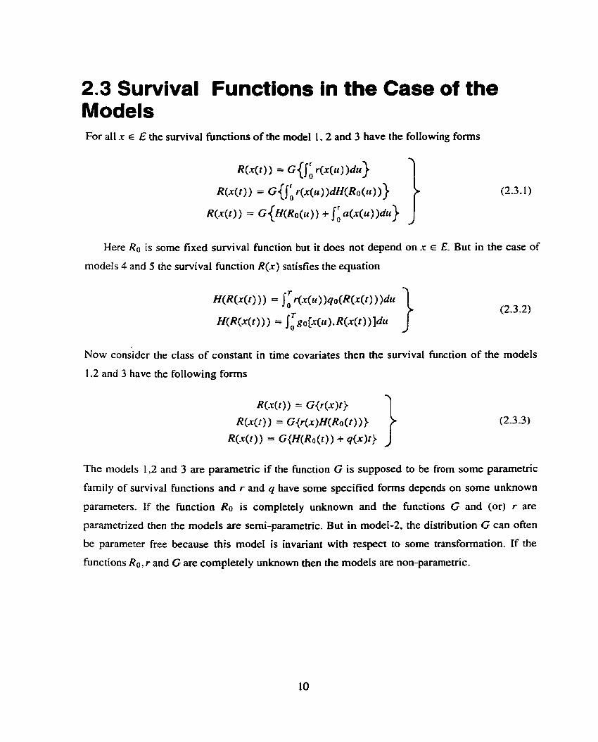
2.3 Survival Functions in the Case of the Models For al1 x E E the swvival functions of the mode1 1 ,2 and 3 have the following forms

Here Ro is some fixed survival hnction but it does not depend on x E E. But in the case of

models 4 and 5 the survival hnction R(x) satisfies the equation

Now consider the class of constant in time covariates then the survival hinction of the models

1.2 and 3 have the following forms

The modeIs 1,2 and 3 are parametric if the function G is supposed to be frorn some paramevic

family of survival functions and r and q have some specified forms depends on some unknown

parameters. If the function Ro is completely unknown and the functions G and (or) r are

pararnetnzed then the models are semi-parameuic. But in model-2, the distribution G can often

be parameter free because this mode1 is invariant with respect to some transformation. If the

functions Ro, r and G are completely unknown then the models are non-paramemc.

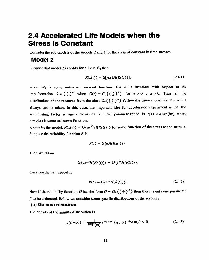
2.4 Accelerated Life Models when the Stress is Constant Consider the sub-models of the models 2 and 3 for the class of constant in time stresses.

Model-2 Suppose that model 2 is holds for al1 x E Eo then

where Ro is some unknown survival function. But it is invariant with respect to the

transformation S = ($)' when G(t) = G O ( ( $ ) = ) for O > 0 . a > O. Thus al1 the

distributions of the resource from the class Go (($) ') follow the sarne model and 6 = a = 1

always can be taken. in this case, the important idea for accelerated experirnent is Aat the

accelerating factor is one dimensional and the paramemzation is r(x) = aexp(6z) where

z = z(x) is some unknown function.

Consider the model. R(x(r ) ) = G { a e f i ~ ( ~ ~ ( t ) ) ) for some hinction of the stress or the stress r.

Suppose the reliability function R is

Then we obtain

therefore the new model is

Now if the reliability hinction G has the form G = Ga ( ( $ ) then there is only one parameter

p to be estimated. Below we consider some specific distributions of the resource:

(a) Gamma resource The density of the gamma distribution is

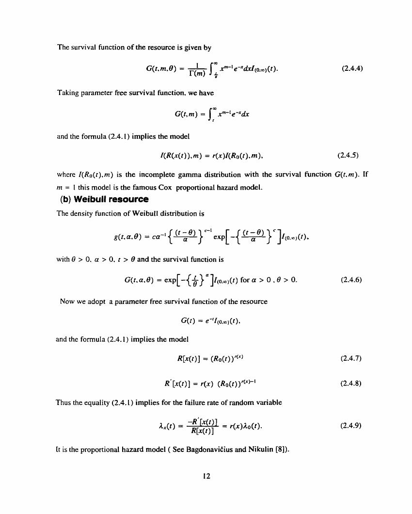
The survival function of the resource is given by

Taking parameter free survival function. we have

and the formula (2.4.1) impiies the model

where I(Ro(r) .m) is the incomplete gamma distribution with the survival Function G(t.m). If

m = 1 this model is the farnous Cox proportional hazard model.

(b) Weibull resource The density tünction of Weibull distribution is

with 8 > O, a > O, r > 8 and the survival function is

G(t.a.0) = exp[-($1 a ] ~ ( o . m l ( r ) for a > O . O > 0.

Now we adopt a parameter free survival function of the resource

G(t) = ~ - ' I ( o . ~ ) ( t ) ,

and the formula (2.4.1) irnplies the model

R[x(r ) J = (Ro ( r ) ) w

R' [ ~ ( r ) 1 = r (x) (Ro(t) )flX)-'

Thus the equality (2.4.1) implies for the failure rate of random va-iable

It is the proportional hazard model ( See Bagdonavitius and Nikulin [8]).

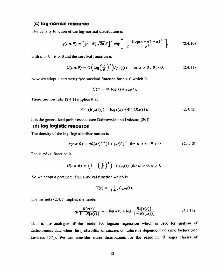
(c) log-normal resource The density function of the log-normal distribution is

1 (iog(x-O) -a>' g(r. a.0) = [ ( r - O) &6]-' exp[-2 (2.4.10)

o

with a > 0 . 8 > O and the survival function is

Now we adopt a parameter free survivai function for t > O which is

G(t ) = @(log(r) )i(o.m)(t).

Therefore formula (2.4.1) implies that

4-1 (R[x( t ) ] ) = log r(x) + W1 (Ro(t)) .

It is the generalized probit model (see Dabrowska and Doksum [26]).

(d) log logistic resource The density of the tog- logistic distribution is

g(t. a. 0 ) = a ~ ( a t ) ~ - ' ( 1 + (ar )~)" for a > 0 , O > 0

The survival function is

G(r.a,O) = ( 1 c (k) a ) - l l ~ O . ~ ) ( t ) for n > O. 0 z O.

So we adopt a parameter free survival function which is

The formula (2-4.1) implies the model

This is the analogue of the model for

dichotomous data when the probability of

-log r(x) + log Ro [ x u ) 1 1 - Ro[x(t)l -

logistic regression which is used for analysis of

success or failure is dependent of same factors (see

Lawless [57]). We can consider other distributions for the resource. If larger classes of

13

distributions of the resource are considered then the more general semi-parameuic models

including known models can be obtained.

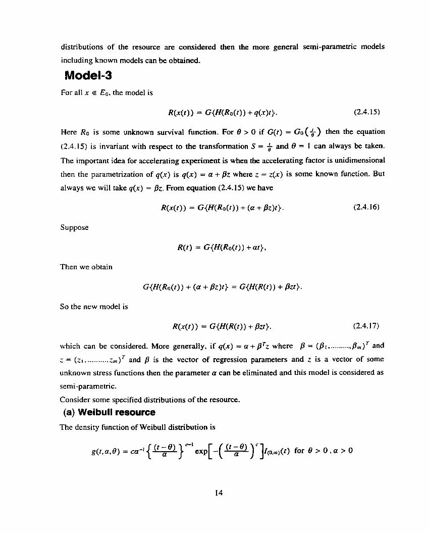
Model-3 For al1 x E Eo, the model is

Here RO is some unknown survival hinction. For 0 > O if G(t ) = Go($-) then the equation

(2.4.15) is invariant with respect to the transformation S = $ and 0 = i can always be taken.

The important idea for accelerating experiment is when the accelerating factor is unidimensional

then the parametrization of q(x) is q(x) = n + pz where z = z(x) is some known Function. But

always we will take q(x) = pz. From equation (2.4.15) we have

Suppose

Then we obtain

C{H(Ro ( r ) ) + (a t f i ) [ ) = G{H(R(t) ) + m). So the new model is

which can be considered. More generally. if q ( r ) = a + pTz where P = (Bi. .......... p,)* and

- - - (z i . - . . - - - - . - . ;m)r and p is the vector of regression parameters and z is a vector of some

unknown stress functions then the parameter a can be eliminated and this model is considered as

serni-parametric.

Consider some specified distributions of the resource.

(a) Weibull resource The density hnction of Weibull distribution is

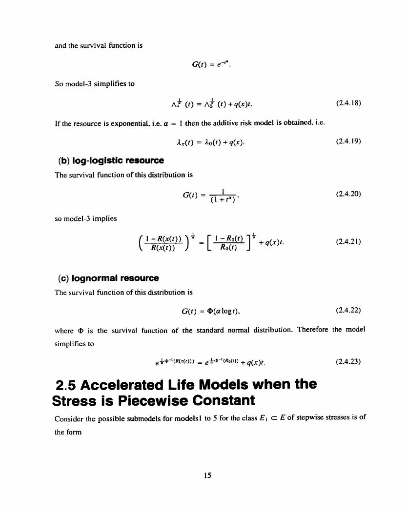
and the sumival function is

G(t) = e-fa.

So model-3 simplifies to

i I Ar" ( t ) = Ag ( r ) + q(.r)t. (2.4.18)

If the resource is exponential, i.e. a = 1 then the additive risk mode1 is obtained. Le.

(b) log-logistic resource The survival function of this distribution is

(c) lognormal resource The survival function of this distribution is

G(t ) = @(a log t), (2.4.22)

where 0 is the sumival function of the standard normal distribution. Therefore the mode1

simplifies to

eL*-'(~(-W))) = e+@-'(Ro(t)) + &p. (2.4.23)

2.5 Accelerated Life Models when the Stress is Piecewise Constant Consider the possible submodels for modelsl to 5 for the class El c E of stepwise stresses is of

the form

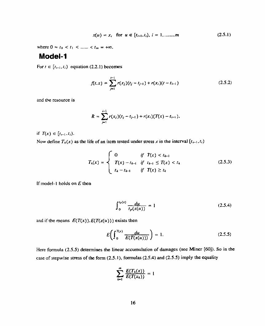
where O = t o < t l < .-...- < t , = +a.

Model-1 For t E [r i - , , t ; ) equation (2.2.1) becomes

and the resource is

if T(x ) E [ r i - ! . r , ) .

Now de fine Tk(x) as the life of an item tested under stress x in the interval [fi-1. f i )

If model-1 holds on E then

and if the means E(T(x)) , E(T(x(t2))) exists then

Here formula (2.5.5) determines the linear accumulation of damages (see Miner [60]). So in the

case of stepwise stress of the form (2.5.1 ), formulas (2.5.4) and (2.5.5) imply the equality

and

if tp(-r) E [ t r - , , tk ) .

The inequality (2.5.6) is called Peshes-Stepanova model (see Kartashov [54]). These formulas

can be used for estimation of the mean life under normal stress from the data of accelerated

testing.

Model-2 Consider mode[-2 holds on E, then

where x is of the forrn in (2.5.1). Then fort < ri we have

This equality can be used for the estimation of the survival hinction under the normal stress

fiom accelerated life experiments.

Modeld Consider model-3 to be m e on E, then

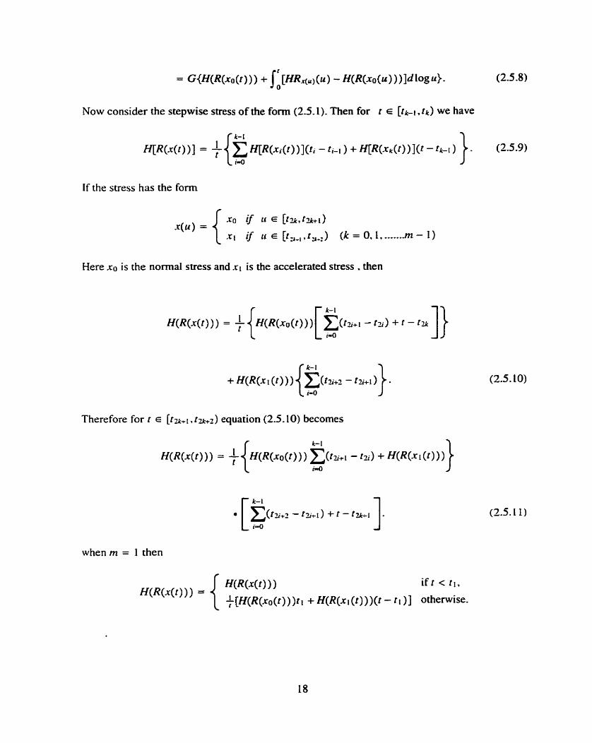
Now consider the stepwise stress of the fonn (2.5.1). Then for r E [tk-1. t k ) we have

f k-t 7

If the stress has the form

Here .CO is the normal stress and xi is the accelerated stress . then

There fore for r E [ t s , l , t ~ + l ) equation (2.5.10) becomes

when m = 1 then

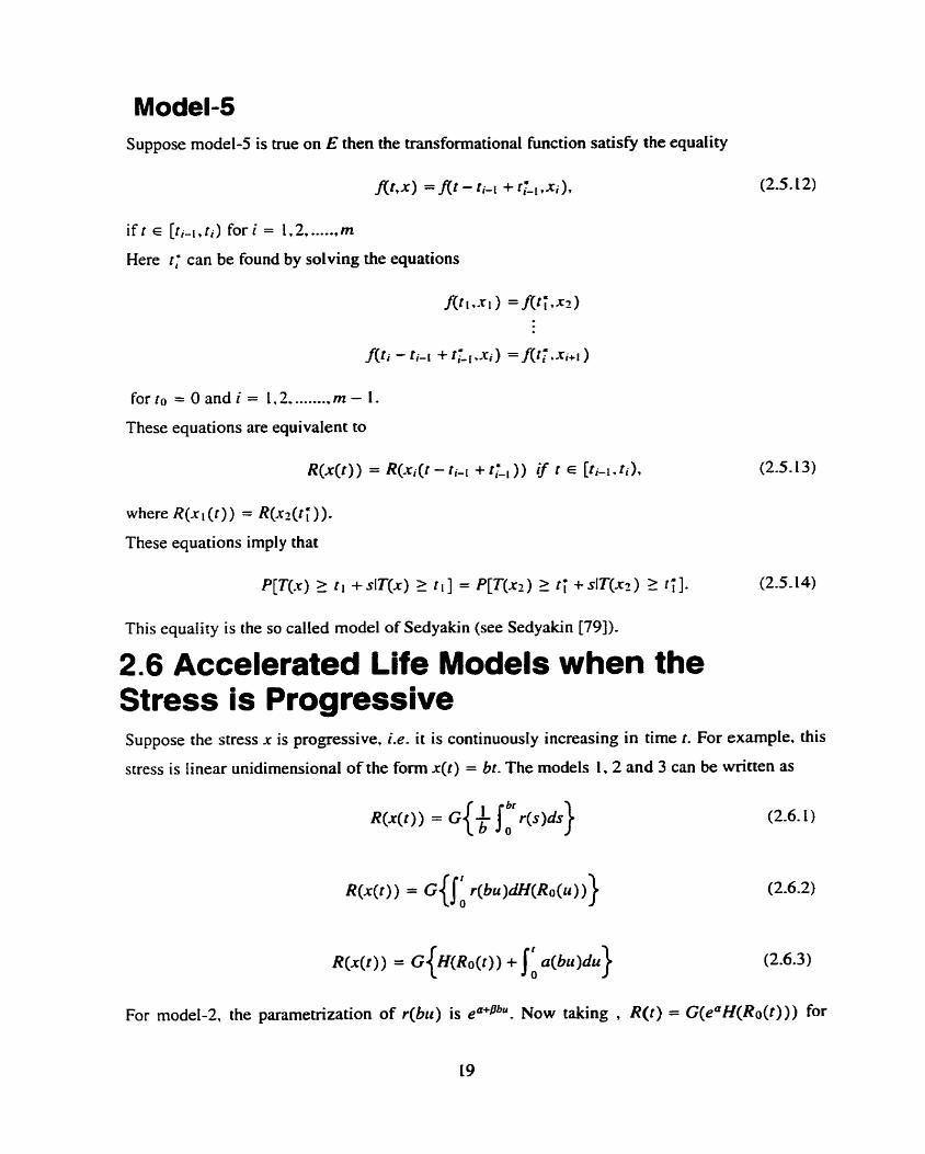
Suppose model-5 is tme on E then the transformational fùnction satisQ the equality

i f t E [ti-l.ti) fo r i = 1,2, ....., m

Here r ; can be found by solving the equations

fort0 = O a n d i = 1.2 ........, m - 1.

These equations are equivalent to

where R(x (t)) = R(-rz(ti ))-

These equations imply that

This equality is the so called mode1 of Sedyakin (see Sedyakin [79]).

2.6 Accelerated Life Models when the Stress is Progressive Suppose the stress x is progressive, i.e. it is continuously increasing in time t . For exarnple. this

stress is Iinear unidimensional of the forrn x(t) = bt. The models 1.2 and 3 can be written as

For model-2, the parametrization of r(bu) is ea+pbu. Now taking , R(r) = G(eaH(Ro(t))) for

eiiminating a, the mode1 is

R(x(i) ) = G{I' O e"KdH(Ra(u)))-

Sirnilarly. model-3 is

R(x(r) ) = G{H(Ro(r ) ) + Pb?').

3 Possible Survival Distributions and Their Propert ies 3.1 Introduction

In this chapter. we consider some statistical distributions that are used to describe survival cimes

in accelerated life testing. The distributions discussed in this thesis are the Gamma. Log-normal

and Inverse Gaussian.

Consider a set of observations from a population. The natural question arises about the nature of

the parent population. The ctear idea is provided by the fiequency polygon or frequency curve.

But the information may be totally inadequate and unreliable. i.e. the sarnple observations may

not cover the entire range of the parent distribution. Basically. an unusually high frequency in

any one class may anse and the frequency curve may completely out of shape. In order to

determine the fiequency curve, we will have to make use of the technique of curve fitting to the

given data. Some standard distributions rnay be tried and the best fitting distribution may be

selected. Below. some important properties of common distri butions used in survival and

reliability analysis are described.

3.2 Gamma distribution 3.2.1 Gamma distribution as a model for failure times

In this thesis we consider the Gamma distribution as a model for failure times. We consider here

the Gamma distribution because of its appealing features:

(i) It accommodates a variety of shapes similar to the Weibull, Inverse Gaussian and log-normal

distribution.

(ii) This distribution has the structure of an exponential family and its many properties are

associated with sampling distributions.

(i i i ) Its derivation From a stochastic formulation of the failure process provides a physical

support to its exact fit.

In this thesis, we consider a reciprocal linear regression model for the mean of the Gamma

distribution. We consider the following situation. Suppose n objects are subjected to stress levels

x 1 ,xz, .......... x, and there failure tirnes are obsewed. Each object has â characteristic outset

which we take to be the same. The stress levels signify the accumulation of the fatigue process at

different levels. The Gamma distribution is a good competitor to other well known survival

distributions such as the Inverse Gaussian. the WeibuII and the Log normal.

3.2.2 Properties The general form for the p,d.f, of a random variable x has a Gamma distribution

where r and p are Iocation and scale paranieter respectiveiy and a determines the shape of the

p.d.f. This distribution is Pearson's type 3. The standard form of this distribution is obtained by

putting P = 1 and r = O which is given by

+ra- 1 -x

f w = ra for x 2 O.

If n = 1. the Gamma distribution reduces to the exponentiai distribution. If a is a positive

integer. the Gamma dismbution is sometimes called a special Erlangian distribution. Put y = -,r

in (3.2.2.1) and (3-2.2.2) then,

(-y) e~ MY) = Fa for y I 0.

(3.2.2.3) and (3.2.2.4) are also Gamma distributions rarely considered and not discussed hrther

here.

The cumulative distribution hnction of (3.2-2.2) is

which is called an incomptete Gamma function ratio but

is sometimes called incomplete Gamma function. Pearson

(3.2.2.6)

[73] found it more convenient to use

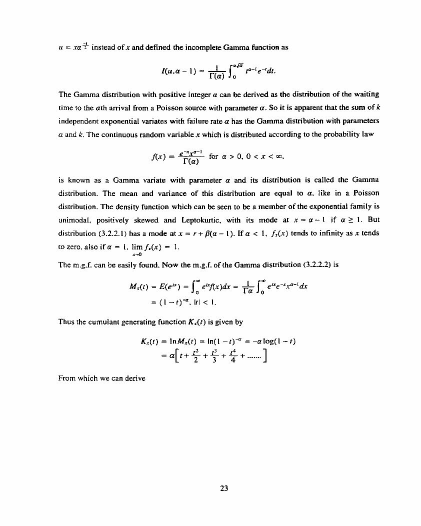
rt = .rcr 2 instead of x and defined the incomplete Gamma fùnction as

The Gamma distribution with positive integer a can be derived as the distribution of the waiting

time to the a th arriva1 fiom a Poisson source with parameter a. So it is apparent that the sum of k

independent exponential variates with failure rate a has the Gamma distribution with parameters

a and k. The continuous random variable x which is distributed according to the probability law

for a > 0, O c x < m.

is known as a Gamma variate with parameter u and its distribution is called the Gamma

distribution. The mean and variance of this distribution are equal to a. like in a Poisson

distribution. The density fùnction which can be seen to be a member of the exponential family is

unimodal, positively skewed and Leptokurtic, with its mode at x = a - 1 if a 2 1. But

distribution (3-2.2.1) has a mode a t x = r + &a - 1 ). If a < 1, f r ( x ) tends to infinity as x tends

to zero, also if a = 1, lim Jr (x ) = 1. .=-O

The m.g.f. can be easily found- Now the m.g.f- of the Gamma distribution (3.2.2.2) is

Thus the curnuIant generating tünction K.,(t) is given by

From which we can derive

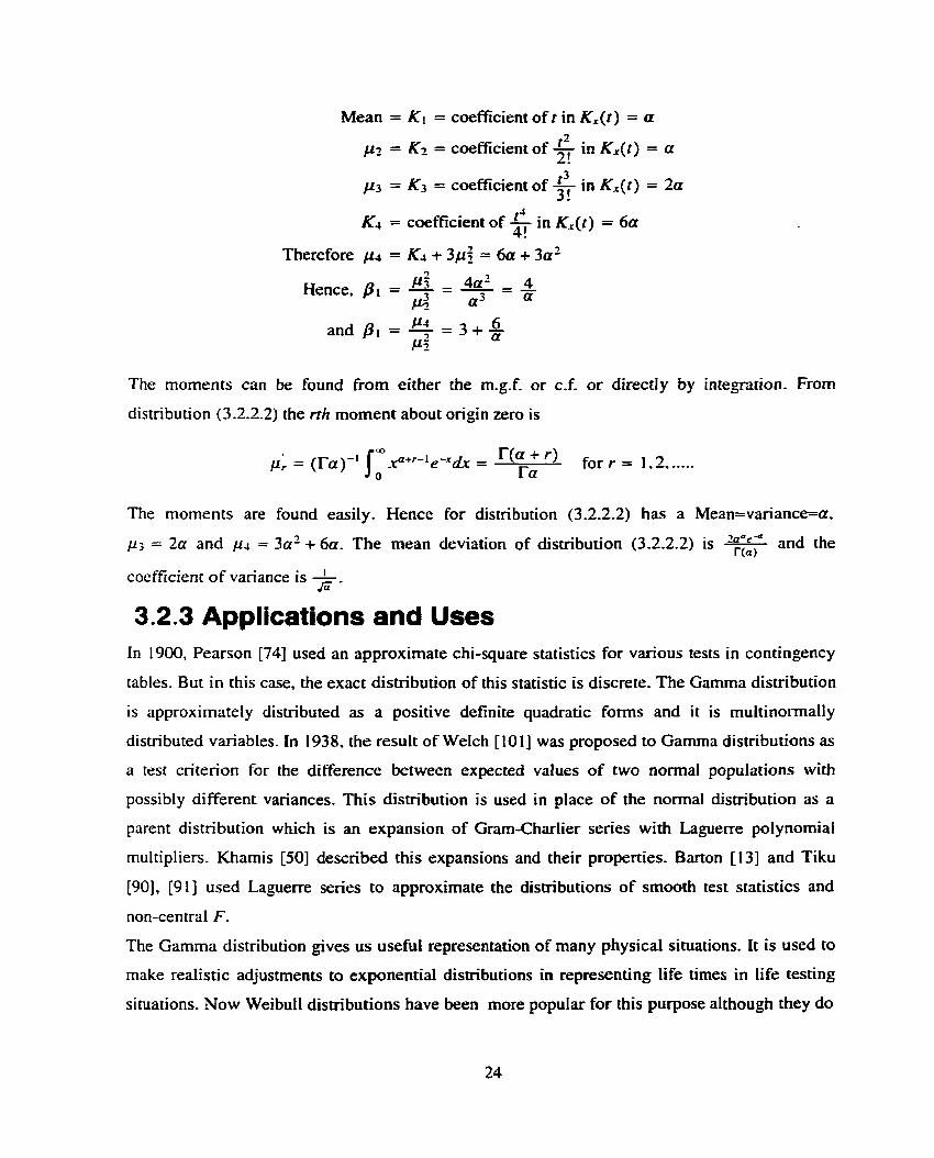
Mean = Kt = coefficient of t in K,(t) = a

pz = Kt = coefficient of 2 in K x ( t ) = a 2! t 3

p3 = K3 = coefficient of - in K.&) = 2a 3! tJ KJ = coefficient of - in Kx( t ) = 6a 4!

Therefore P J = Ka + 3p3 = 6a + 3a2 P 4a2 4 - - Hence, = 7 = - - k- a3 a

P4 6 and pi = 7 = 3 + , PI

The moments c m be found from either the m.g.f. or c f - o r directly by intebgation. From

distribution (3.2.2.2) the rth moment about origin zero is

OD

= ( ~ a ) - ' J - tmr-l e-ILk = T ( a -t r ) Ta for r = 1.2. ,....

O

The moments are found easily. Hence for distribution (3.2.22) has a Mean=variance=a.

ps = 2a and p4 = 3a2 + 6a . The mean deviation of distribution (3.2.2.2) is and the

coefficient of variance is f i -

3.2.3 Applications and Uses In 1900, Pearson [74] used an approximate chi-square statistics for various tests in contingency

tables. But in this case, the exact distribution of this statistic is discrete- The Gamma distribution

is approximately distributed as a positive definite quadratic f o m s and it is multinormally

distributed variables. In 1938, the result of Welch [IO11 was proposed to Gamma distributions as

a test criterion for the difference between expected values of two normal populations with

possibly different variances. This distribution is used in place of the normal distribution as a

parent distribution which is an expansion of Gram-Charlier series with Laguerre polynomial

multipliers. Khamis [50] described this expansions and their properties. Barton 1131 and Tiku

[90], [91] used Laguerre series to approximate the distributions of smooth test statistics and

non-central F.

The Gamma distribution gives us usefûl representation of many physical situations. It is used to

make realistic adjustments to exponential distributions in representing life times in Iife testing

situations. Now Weibutl distributions have k e n more popular for this purpose although they do

not provide a permanent solution. Weibull families have simple Forms of the faiiure rate

function. Also the sum of independent exponentially distributed random variables represents a

Gamma distribution which leads to the appearance in the theory of random counters and other

related topics in associated with random process in rneteorological precipitation process. This

was discussed by Kotz Neumann [49], Das [25].

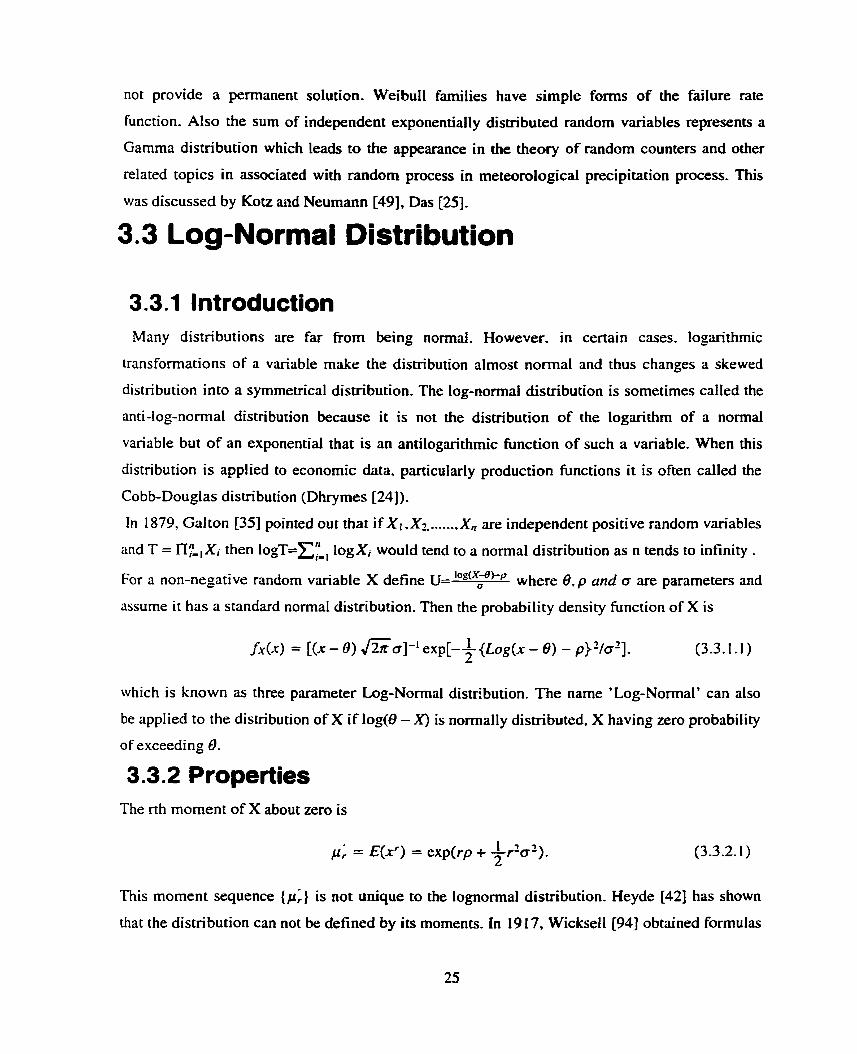
3.3 Log-Normal Distribution

3.3.1 Introduction Many distributions are far from being normd. However. in certain cases. logan-thmic

transformations of a variable make the distribution almost normal and thus changes a skewed

distribution into a symmetrical distribution. The log-normal distribution is sometimes called the

anti-log-normal distribution because it is not the distribution of the logarithrn of a normal

variable but of an exponential that is an antilogarithmic function of such a variable. When this

distribution is applied to economic data. particularly production functions it is often called the

Cobb-Douglas distnbution (Dhrymes [24]).

In 1879, Galton [35] pointed out that if X i ,X2-......,X, are independent positive random variables

and T = nL1X, then IO~T=C;_, logXi would tend to a normal distribution as n tends to infinity .

For a non-negative random variable X define U= 'Og'X$)-p where 0, p and o are parameters and

assume it has a standard normal distribution. Then the probability density function of X is

which is known as three parameter Log-Normal distribution. The name 'Log-Normal' can also

be applied to the distri bution of X if log(@ - X) is normally distri buted, X having zero probabiiity

of exceeding 8.

3.3.2 Properties The rth moment of X about zero is

This moment sequence (pi) is not unique to the lognormal distribution. Heyde [42] has s h o w

that the distnbution can not be defined by its moments. In 19 17, Wicksetl 1941 obtained formulas

for the higher moments while Van Uven [92], [93] considered transformations to nomality from

a more general point of view. The mean of this distribution is

and when w = en' the lower order central moments are

p2 = e'~e"2 (eu2 - 1) = ~ ( o - l ) eZp

pj = - 1 )'(o + I )e3p

pi = 02(o - 1)'(04 + h3 + 3m2 - 3)e4P .

The coefficient of variation is (w - 1) '". This distribution of X is unimodal and its mode is

and median of X is e".

.*. Mean > Median > Mode.

As o -. O or 6 to infinity the standard Log- Normal distribution tends to a unit normal

distribution. Acnially as c increases. the log-normal distribution rapidly becomes markedly

non-nomal. Wise [95] has shown that the probability density function of the two parameter

distribution has two points of inflection at x = exp[p - 4$- f a 1 + -a2- 1. - r 3.3.3 Applications and Uses

The Log-normal distribution is usually represented as the distribution of vm-ous economical

variables (see Gibrat [38], [39]). Gaddum [36] and Bliss (141 found that the distribution of the

critical dose for a number of f o m s of dmg application could be represented with adequate

accuracy by a two parameter Log-norrnal distribution. In 1937- 1940, Cochran [ 171, Wiliiams

1961 [97], Grundy [40], Herdan 1441. [45] and Pearce [75] described the use of the Log-normal

distribution in agricultural, entornoiogical and literary research. Wu [98] has s h o w that

Log-normal distributions can arise as limiting distributions of order statistics if sample size and

order increase in certain relationships. Kolmogrov [53], Tomlinson 1881, Oldham 1721 applied

this distribution of particle sizes in naniral aggregates and in the closely related distribution of

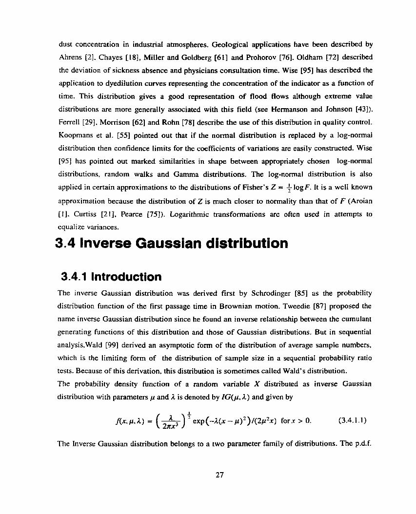
dust concentration in industriai atmospheres. Geological appkations have been described by

Ahrens [2] , Chayes [ l 81, Miller and Goldberg [6 11 and Prohorov [76], Oldham [72] described

the deviation of sickness absence and physicians consultation time. Wise [95] has described the

application to dyedilution curves representing the concentration of the indicator as a function of

time. This distribution gives a good representation of flood fiows although extreme value

distributions are more generally associated with this field (see Hermanson and Johnson [43]).

Ferre11 [29], Momson [62] and Rohn [78] describe the use of this distribution in quality control.

Koopmans et aI- [55] pointed out that if the normal distribution is replaced by a log-normal

distribution then confidence Iimits for the coefficients of variations are easily constructed- Wise

(951 has pointed out marked similarities in shape between appropriately chosen log-normal

distributions, random walks and Gamma distributions. The log-normal distribution is also

applied in certain approximations to the distributions of Fisher's Z = f log F. It is a well known - approximation because the distribution of Z is much closer to normality than that of F (Aroian

[ i l . Curtiss [21], Pearce 1753). Logarithmic transformations are often used in attempts to

equalize variances.

3.4 Inverse Gaussian distribution

3.4.1 Introduction The inverse Gaussian distribution was derived first by Schrodinger [85] as the probability

distribution function of the first passage time in Brownian motion. Tweedie [87] proposed the

name inverse Gaussian distribution since he found a n inverse relationship between the cumulant

generating functions of this distribution and those of Gaussian distributions. But in sequential

analysis,Wald [99] derived an asymptotic form of the distribution of average sample numbers,

which is the limiting form of the distribution of sample size in a sequential probability ratio

tests. Because of this denvation, this distribution is sometimes called Wald's distribution.

The probability density function of a random varÏable X distributed as inverse Gaussian

distribution with parameters p and A is denoted by IG(p, A ) and given by

The Inverse Gaussian distribution belongs to a two parameter family of distributions. The p.d.f.

of this distribution can be represented in several different forms each of which would be

convenient for some purpose. Another important form c m be obtained by a Weiner process w, in

one dimension with positive drift v and w(0) = O. The time T which is required for the Weiner

process to reach an arbitrary real value a, is a random variable with d.f.

, This form is a reparametrization of the p.d.f. in (3.4.1.1) obtained by putting p = 5 and A = " g2

where a is specified. There are various other representations of the density hnction but we will

use the p-d-f- in (3-4.1 -1).

3.4.2 Properties The mean and variance of this distributions are p and $ respectively. This distribution is

unimodal and positiveiy skewed, with mode

and its shape depends only on the value of 4 = +. The cumulant generating function of this

distribution is obtained as

Therefore the first four cumulants are

Kr = p

Kz = é A

K3 = À'

1 5 ~ ~ K', = - ~3 - Generally, for r >: 2, Tweedie 1131 found the formula for the rth cumulant Le-

Kr = 1.3.5 ......( 2r - 3)4-(r-1) where # = +. The characteristic function of this distribution is

{ ( (l-2gL)+)}. @,(t) = E[eh] = exp 1 -

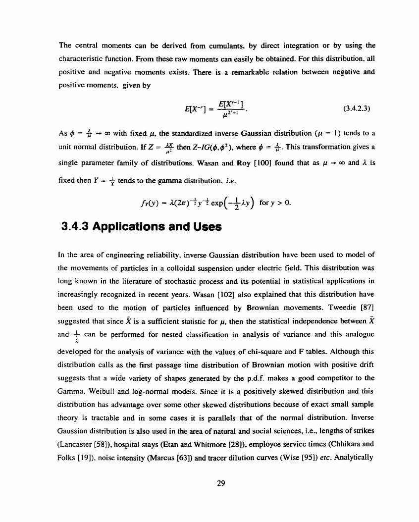
The central moments can be derived from cumulants, by direct integration or by using the

characteristic function. From these raw moments can easily be obtained. For this distribution, al1

positive and negative moments exists. There is a remarkable relation between negative and

positive moments. given by

As # = 4 -. with fixed p. the standardized inverse Gaussian distribution (p = 1 ) tends to a

unit normal distribution. If Z = then 2-IG(#.gZ), where 4 = +. This transfomation gives a

single parameter family of distributions. Wasan and Roy [ I O ] found that as + a and A is

fixed then Y = tends to the gamma distribution. i.e.

-1 I f~(y) = 4211) 2 y 2 exp(--$Ly) for y > 0.

3.4.3 Applications and Uses

In the area of engineering reliability, inverse Gaussian dismbution have been used to mode1 of

the movements of particles in a colloidal suspension under electric field. This distribution was

long known in the litenture of stochastic process and its potential in statistical applications in

increasingly recognized in

been used to the motion

suggested that since x is a

and + can be perforrned L

recent years. Wasan [102] also explained that this distribution have

of particies influenced by Brownian rnovements. Tweedie 1871

sufficient statistic for p, then the statistical independence between x for nested classification in analysis of variance and this analogue

developed for the anaIysis of variance with the values of chi-square and F tables. Although this

distribution calls as the first passage time distribution of Brownian motion with positive drift

suggests that a wide variety of shapes generated by the p.d.f. makes a good competitor to the

Gamma. Weibull and log-normal models. Since it is a positively skewed distribution and this

distri bution has advantage over some other skewed distri butions because of exact small sample

theory is tractable and in some cases it is parallels that of the normal distribution. Inverse

Gaussian distribution is also used in the area of natural and social sciences. i.e., lengths of strikes

(Lancaster [58]), hospital stays (Etan and Whitmore [28]), employee service times (Chhikara and

Folks [19]). noise intensity (Marcus (631) and tracer dilution curves (Wise [95]) etc. Analytically

inverse Gaussian distribution is suificient to use for curve fitting but its scientific interest is

limited. This distribution serves as a good model for accelerated life tests. Banne j ee and

Bhattacharyya [LOI applied this distribution in marketing research and Chhikara and Folks [20]

consider applications of IG in life testing. Bhattacharyya and Fries [5j argue that IG is more

appropnate than the Birbaum Saunders fatigue distribution and Chhikara and Gultman [22] gives

sequential and Bayesian prediction limits. So the IG widely used tool in reliability theory.

Gerstein and Mandelbred [41] showed that the IG model provides a good fit for the spontaneous

activity of several neurons in the auditory of a cat and explained that by introducing a time

varying drift for the Brownian motion they replicate the behaviors of one of the neurons

subjected to periodic stimuli of vanous fiequencies, Weiss Il031 has g v e n a review of the

various types of random walk models for physical systems. Bachelier [12] used IG in stock

prices. Recently Banne jee and Bhattacharyya [ 101 used this IG model in renewal process and

Whitmore Cl041 used this model to find labour turnover in marketing and labour research area.

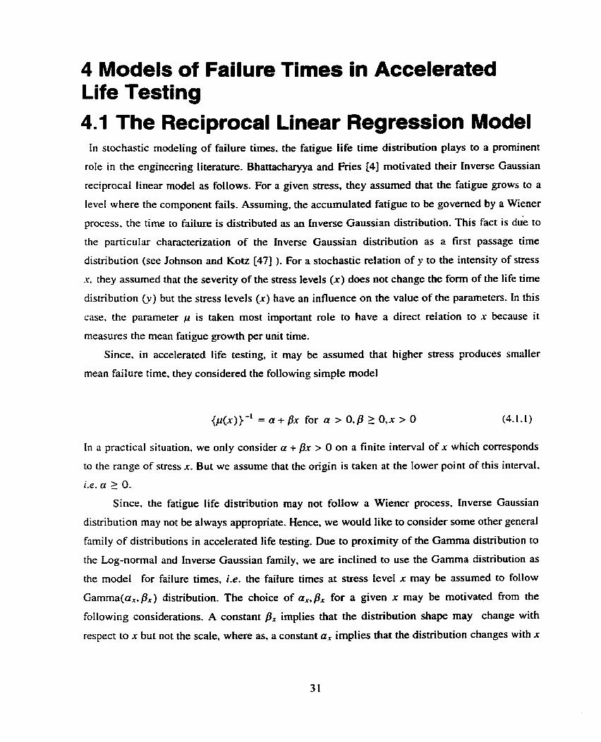
4 Models of Failure Times in Accelerated Life Testing 4.1 The Reciprocal Linear Regression Model

In stochastic modeling of failure times, the fatigue life tirne distribution plays to a prominent

role in the engineering literature. Bhattacharyya and M e s [4] motivated their Inverse Gaussian

reciprocal linear mode1 as follows. For a given stress, they assumed that the fatigue grows to a

level where the component fails. Assuming, the accumulated fatigue to be governed by a Wiener

process. the time to Mure is distributed as an Inverse Gaussian distribution. This fact is due to

the particular characterization of the Inverse Gaussian distribution as a f m t passage time

distribution (see Johnson and Kotz [47] ). For a stochastic relation of y to the intensity of stress

.r, they assumed that the severity of the stress levels (x) does not change the form of the life time

distribution (y) but the stress levels ( x ) have an influence on the value of the parameters. In this

case. the parameter y is taken most important role to have a direct relation to x because it

measures the mean fatigue growth per unit time.

Since. in accelerated life testing. it may be assumed that higher stress produces smaller

mean failure time. they considered the following simple model

(p(~))-' = a + f i for a > 0.P 2 0.x > O (4-1.1)

In a practical situation, we only consider a + Px > O on a finite interval of x which corresponds

to the range of stress x. But we assume that the origin is taken at the lower point of this interval,

i.e. a 2 O.

Since, the fatigue life distribution may not follow a Wiener process. Inverse Gaussian

distribution may not be always appropriate. Hence. we would like to consider some other general

farnily of distributions in accelerated life testing. Due to proximity of the Gamma distribution to

the Log-nomial and Inverse Gaussian family. we are inclined to use the Gamma distribution as

the model for failure times, i.e. the failure times at stress level x may be assumed to follow

Gamma(a.&) distribution. The choice of ax,px for a given x may be motivated from the

following considerations. A constant Px implies that the distribution shape may change with

respect to x but not the scale, where as. a constant a, implies that the distribution changes with x

according scale changes. Moreover. since, p, = a,/3,, the mean failure time at level x is

considered to be a decreasing function of x, a general mode1 for p, may be given by

where g is an increasing Function. assurning that a, is decreasing in x for fixed Px and Px is

decreasing in x for fixed a,. For simplicity, we consider the following choices

FirstModel a, = (no + a N)-'

SecondModel Px = ( B o + B lx)-'

ThirdModel a, = [a0 + a 1 ( f ) ] FourthModel P, = [BO + Pi (a)]

The method of estimation involving these models is maximum likelihood. a general treatment of

which is given in the following section.

4.2 Introduction of ML Method

Method of Maximum Likelihood is the most widely used method of estimation which was

initially formulated by C. F. Gauss but as a general method of estimation was first introduced by

Professor R. A. Fisher. Method of maximum likelihood has the following attractive features:

i) Generally it is a simple procedure, although the computational problems may not always be

simple.

ii) The asymptotic propenies of maximum likelihood estimators for under certain regularity

conditions make their use desirable.

iii) Maximum likelihood estimation affords a rather general methods of estimation of parmeters

of suwival distribution's even when observations are censored for example one can in most

instances obtain the maximum likelihood estimators of the parameters of the survival

distribution.

For some models. explicit solution of the maximum likelihood estimators rnay be possible.

However for other models solutions can not be obtained explicitly. For this reason, there are two

computational methods of finding maximum likelihood estimators such as Newton-Raphson

method and Scoring method, These are described in the next section.

4.3 Computational Aspects of ML Method Let us consider a random sample of n observations Xi. ..., X, fiom a population with density

function flx.8). The joint density function of sample values when regarded as a hinction of

unknown parameter 6 is called likelihood fiinction and is denoted by

The principle of maximum likelihood consists in finding an estimator of the parameter which

maximizes L for variations in the parameter. Thus if there exists a Function 8 = 8(xi..-..r,J of the

sample values which maxirnizes L, then 8 is to be taken as estimator of 8. Thus is the solution

of the equation = O subject to the condition that $$ < O Le. 0 consists of a single parameter.

Since L > O so is logL which shows that L and logL attain their extreme values at the same value

of 8. But i t is more convenient to work with Io&. S o M.L. estimator is generally obtained as aogL 2' IO& the solution of the equation 7 = 0 subject to the condition that 7 < O. For

multiparameter case. the MLETs 3 - --. 8, of B i , - - - , B r are obtained as the solution of the k x k

system of equations, i.e,

A

(See Cramer [ 1 S]).The estirnators (8 i T - - -, O I ) are asymptotically normally distributed with mean

(8 I . - - S . B r ) and variance-covariance matrix Vg (see Rao[77]) where

In cases where it is not possible to obtain Maximum Likelihood Estimators for the parameters of

the distribution then we use numerical techniques. There are two cases of the numerical

techniques

i) No constraints on values of the parameters are assumed.

ii) Parameters are subject to some constraints.

In the second case, maximizing the logarithm of the likelihood hnctions, the constraint is

typicafly as folIows

The value of a parameter must lie in the interior of a particular region and must not lie on the

boundary of that region. Numerical procedures that do not allow for constraints can be used as

long as successive maximum iikelihood estimators lie in the interior of the region.

Here we can describe maximizing techniques that do not consider constraints. These techniques

can be put into direct and indirect classes. In the direct class, starting value is deterrnined which

thought to be a good approximation to the desired value. An example of this class is the method

of steepest ascent or gradient method of Cauchy. In the indirect class. at first the denvatives of

the logarithm of the Iikelihood function with respect to each parameter are obtained and then

equated to zero. Next, the values of the parameters are easily obtained in tenns of the

observations that simultaneously satisQ these equations. Two examples of this cIass are

Newton-Raphson method and the method of Scoring which we investigate below. Rao [77] also

discussed this indirect procedure. Therefore some modem and sophisticated methods are

available for solving non-linear equations of the type which confronts us the Newton-Raphson

method and the Sconng method are very practical to implement and calculations are not

diffrcult.

4.4 Asymptotic Likelihood Maximum Li kelihood

Properties of Maximum Est imators

estimators are the most important methods of estimation because of their

asymptotic properties. Generally, the asymptotic properties for maximum Iiketihood estimates

applies to sarnples with many failures and models that satisQ certain regularity conditions.

Let Xi. ..X, be a random sample of size n from a population with density Cunctionflx). Then the

likelihood function of the sample values xl, ,..,x,, usually denoted by L is given by

The following assumptions are made

i) The first and second order derivatives exist and are continuous functions of 8 in a range %, 210 L including the true value of the parameter for alrnost al1 x. For every û in W. -& < Fi(x) and

CL log L < F7(x) where F i (x) and F2(x) are integrable functions over (-%a).

C-' Iog L 0'10 L ii) 7 exists such that -& < M(x). where E[M(.r)] < k, a positive quantity.

O' log L iii) For every 0 in 9. E(-T) is Rnite and non-zero.

iv) The range of integration is independent of 8. But if the range of integration depends on 0 then

f(.r, 8) vanishes at the extremes depending on 8.

Under the above conditions. the asymptotic properties of the maximum likelihood estimators are

i) MLE is consistent,

ii) It is asymptotically normally disu-ibuted.

1.e.

(iii) It is asymptotically efficient and achieves the Cramer-Rao lower bound for consistent

estirnators.

The second property greatly facilitated hypothesis testing and the construction of interval

estimates and the third property is a particularly powerful result.

Under certain general conditions, maximum Iikelihood estimators possesses some important

theorem which can be helpful to prove the asymptotic properties of maximum likelihood

estimators.

Cramer- Rao Theorem : "With probability approaching unity as n tends to infinity. the

dl0 L likelihood equation -$- = O, has a solution which converges in probability to the truc value

90" (Dugue 1271).

HuzrtrbazarfsTheorem: Any consistent solution of the likelihood equation provides a maximum

of the likelihood with probability tending to unity as the sample size tends to infinit)' (

Huzurbazar [46]).

CrarnerfsTheorern : A consistent soIution of the likelihood equation is asymptotically nomaily n

distributed about the me value Bo. Thus 0 is asymptotically N( Ba. &) (Cramer 1151)- Here

ï(&) is known as the information on 6 supplied by the sample XI, -.-, X,, .

4.5 The Newton-Raphson Method

The Newton-Raphson method is a widely used and often studied method for minimization.

When the derivative of g(8) is a simple expression which can be easily found, the real roots of

the equation g(8) = O can be found rapidly by a process called the Newton-Raphson method

after its discoverers. This method consists in finding an approximate value of the desired root

,oraphically or otherwise and then finding a correction term which must be appiied to the

approximate value to get the exact value of the root. We illustrate this technique by solving first

for a single O and then presenting the case for Oi, i = 1.2. - - -. k. Let

The problem is then to find the value of 8 say 8 such that

Thus 8 is the requisite maximum likelihood estimator of 8. If there is more than one value 8 such that &) = 0. the choice of an initial value is very important. In most cases. the initial

value obtained is in the neighborhood of the maximum likelihood estimator. When in doubt.

consider several different initial values.

If 8 can not be obtained explicitly from solving equation g ( ê ) = O, we rnay attempt a solution

by means of the Newton-Raphson procedure. Suppose be an initial value of 8 and then

finding a correction terni h so that the q a t i o n g ( 8 ) = O becomes g(& + h) = O. Now

expanding + h) by Taylor's theorem we have

Supposing It is very small. we may neglect the ternis containing 12' and other higher powers.

Then we have

x@o) which implies that 11 = -- . ~ ' ( 2 0 )

Then the improved value of the root is given by

Here, 68" is called first approximation of the desired root. Similarly in the same way. the vth

approximation of is given by

w here

Thus. Newton-Raphson method consists of solving each iteration, the equation is

For the next iterate a,+,, the solution takes the form of equation (4.4.2) by replacing by 8,1. and a,-, by 8,. It is evident fiom Newton-Raphson formula that the larger the derivative g' (O).

the smaller is the correction tenn which must be applied to get the correct value of the root. This

means that when the graph of g(8) is nearly vertical where it crosses the x-axis, the correct value

of the root can be found rapidly. But this method should not be used when the graph of g(0) is

nearly horizontal where it crosses the x-axis.

Suppose f ( x ; 8 1, - - - ,Bk) is a density function containing k-parameters 8 1 , - - -, 8 k . k 1 2. A

Furthemore, suppose the maximum likelihood estimators 8 1 . - - -. Or of Bi, ---.Bk are respectively

found by differentiating the logarithm of the likelihood hinction with respect to 91, --- ,& and

then equating to zero and then solving the resulting equations in terms of 0 1 , - - -, 9k. This leads to

a system of k equations in k unknown parameters which can not be solved directly. We then

extend Newton-Raphson method to k-dimensions.

Suppose L(8i,---.8k) be the likelihood function of the k parameters distribution and let the

maximum likelihood estimators of 8 I , - - -,Ok be found by solving simultaneously the vector

equation

where

and

A A

Let us consider the initial estimates of 81, - - - . B k are respectively a i o . +--. 0 m . Then the vth A

iteration of 01,. --- .eh of the solution BI . ---. B k is

A l - 1 A AI

where O = . , - O,l= (êi,,,, ---. êirrl) and gr("') = (gi'l'. - - -.gti)).

g!"" = g i ( B I . , I , - - . .GLL-l) , i = 1.2, ---, k. A ~ S O I l ~ ~ l l ( ~ ~ ) is the k x k rnatnx whose ijrh

element is

for i = 1, -.-,k, j = 1, ---,k.

A

The important part of this method is to choose the initial estimates &o. - - - , O H ) because the

Newton-Raphson method will converge to a value that is not the maximum of likelihood

function [ L ( O 1 . - - -. Oa>]. In 1975, Gross and Clark noted that although this rnethod does net

always guarantee a maximum, i t is a safeguard in that more than one set of initial values is

considered and it means that any particular values in convergence can be uncovered.

4.6 Convergence of the Newton-Raphson Method For considering single O , the Newton-Raphson method formula for finding the roots are

which shows that the Newton-Raphson method is really an iteration method. Since the above

equation can be written syrnbotically in the form

then from the condition of convergency of iteration process, we can say that the

Newton-Raphson rnethod converges when l#'(u,.)l < 1. Hence from equation (4.5.1) we have

Therefore the sufficient condition for convergence is

therefore lg(&&"(8,l) 1 < (g'(ê,-i)) '. Graphical representation has also proved that the Newton-Raphson method converges. See the

figure in next page. We observed that since g'(êo) t O.the tangent Iine is not parallel to the axis- 4 1 )

Where this Iine crosses the 8 axis, we find our next approximation 6 and so on. Generally we

stop our itention procedure when logL(0) stops increasing appreciably. Actually if any value of

two approximations are fairly close. we will make no hirther approximation and accept the last

approximation as the required value o f 8. The value of logL(6) should be calculated at each step

because it permits us to monitor the stopping procedure.

4.7 The Scoring Method The method of scoring is similar to the Newton-Raphson method for obtaining maximum

likelihood estirnates of parameters which was established by C.R. Rao in 1952. Sometirnes

maximum likelihood equations are complicated so that the solutions can not be obtained

directly. For this reason, a great mechanism is introduced by adopting the method known as the

scoring method when the requisite system of equations for solutions is non-linear. In this

method, consider a trial solution and derive Iinear equations for small additive corrections. This

process will continue until the corrections become negligible. The difference between

Newton-Raphson method and scoring method is that the matrix of second derivatives used in the

Newton-Raphson technique is replaced by the matrix of the expected values of second

derivatives in the method of scoring. We discuss this technique by solving first for a single 0 and

then presenting the case for O,; i = 1-2, - - -, k. ClogL Suppose L(0) be the likelihood function of the parameter 8 then 7 is defined as the efficient

OlogL score for 8. Let 00 be the trial value of 8 then expanding 7 by Taylor's expansion, we have

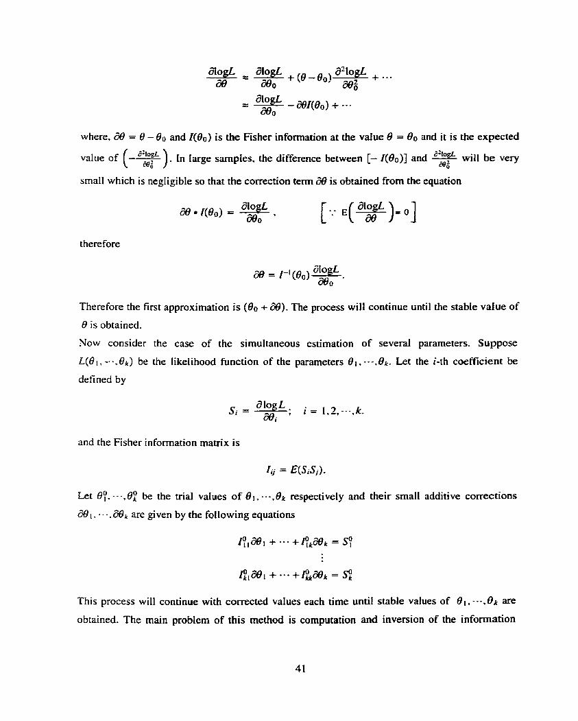
where, 08 = 8 - and [ (O0) is the Fisher information at the value 0 = 80 and it is the expected

Ü'logL d210gl. value of ( -T) . In large samples. the difference between [- I (Oo)] and will be very

small which is negligible so that the correction term 8 is obtained from the equation

therefore

Therefore the first approximation is (Oo + dB). The process will continue until the stable vaiue of

8 is obtained.

Now consider the case of the simultaneous estimation of several parameters. Suppose

L ( 8 1 , -- -, 8k) be the likelihood function of the parameters 8 1 . - - -,O&. Let the i-th coefficient be

defined by

and the Fisher information matrix is

Let 87, - - - , O f be the trial values of O1, - - - , O r respectively and their small additive corrections

ô8 1 . - - -. "en are given by the foliowing equations

This process will continue with corrected vaiues each time until stable values of 8 1, -.-. Or are

obtained. The main problem of this method is computation and inversion of the informafion

matrix at each stage of approximation. But afier some stage, the information matrix may be kept

fixed and only to recalculate the scores. M e n final values are reached at the final stage, the

information matrix rnay be computed at the estirnated values for obtaining the variances and

covariances of estimates. A discussion of the Newton-Raphson method and the method of

scoring is also given by Kale,

4.8 Review of Accelerated Life Testing

This section presents brkf review of the work done in accelerated life testing.

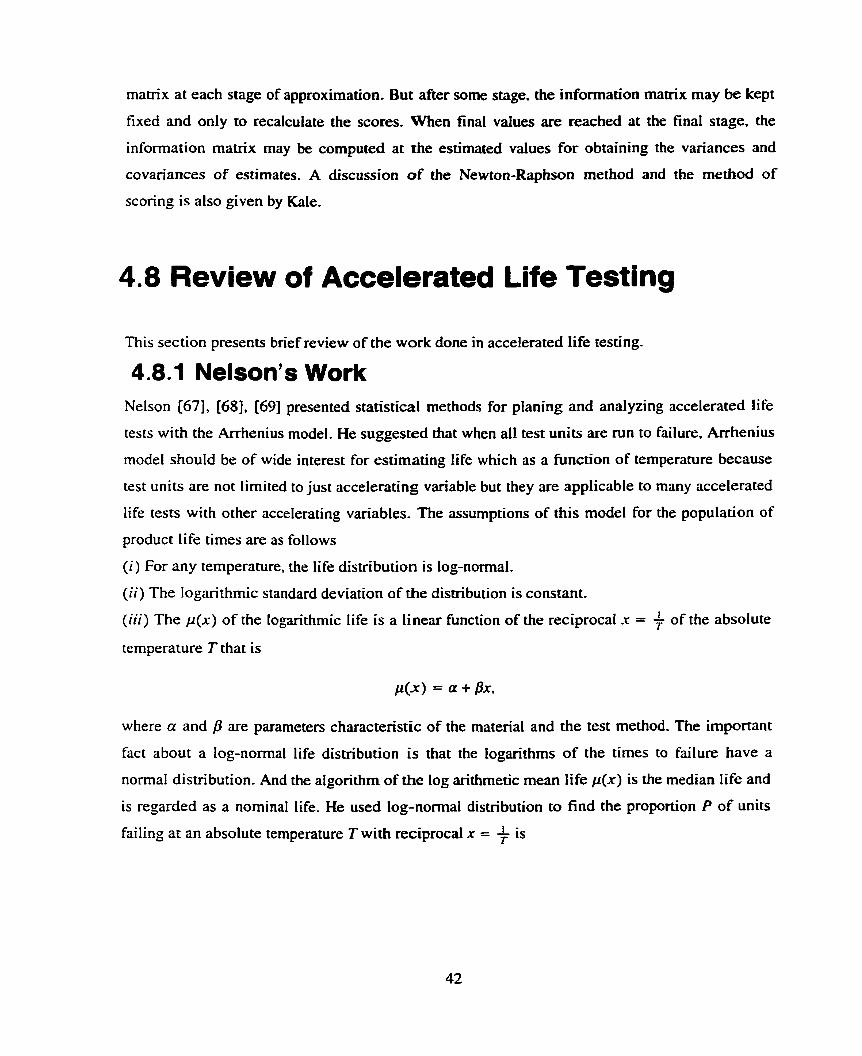
4.8.1 Nelson's Work Nelson [67], [68]. 1691 presented statistical methods for planing and analyzing accelerated Life

tests with the Arrhenius model. He suggested that when al1 test units are run to failure, Arrhenius

mode1 should be of wide interest for estimating life which as a hnction of temperature because

test units are not limited to just accelerating variable but they are applicable to many accelerated

life tests with other accelenting variables. The assumptions of this model for the population of

product life times are as follows

(i) For any temperature, the life distribution is log-normal,

(ii) The logarithmic standard deviation of the distribution is constant.

(iii) The ~ ( x ) of the logarithmic life is a linear function of the reciprocal x = f of the absolute

temperature T that is

where a and p are parameters characteristic of the matenal and the test method. The important

fact about a log-normal life distribution is that the logarithms of the times to failure have a

normal distribution. And the algorithm of the log arithmetic mean life ~ ( x ) is the median life and

is regarded as a nominal life. He used log-normal distribution to find the proportion P of units

failing at an absolute temperature T with reciprocal x = $ is

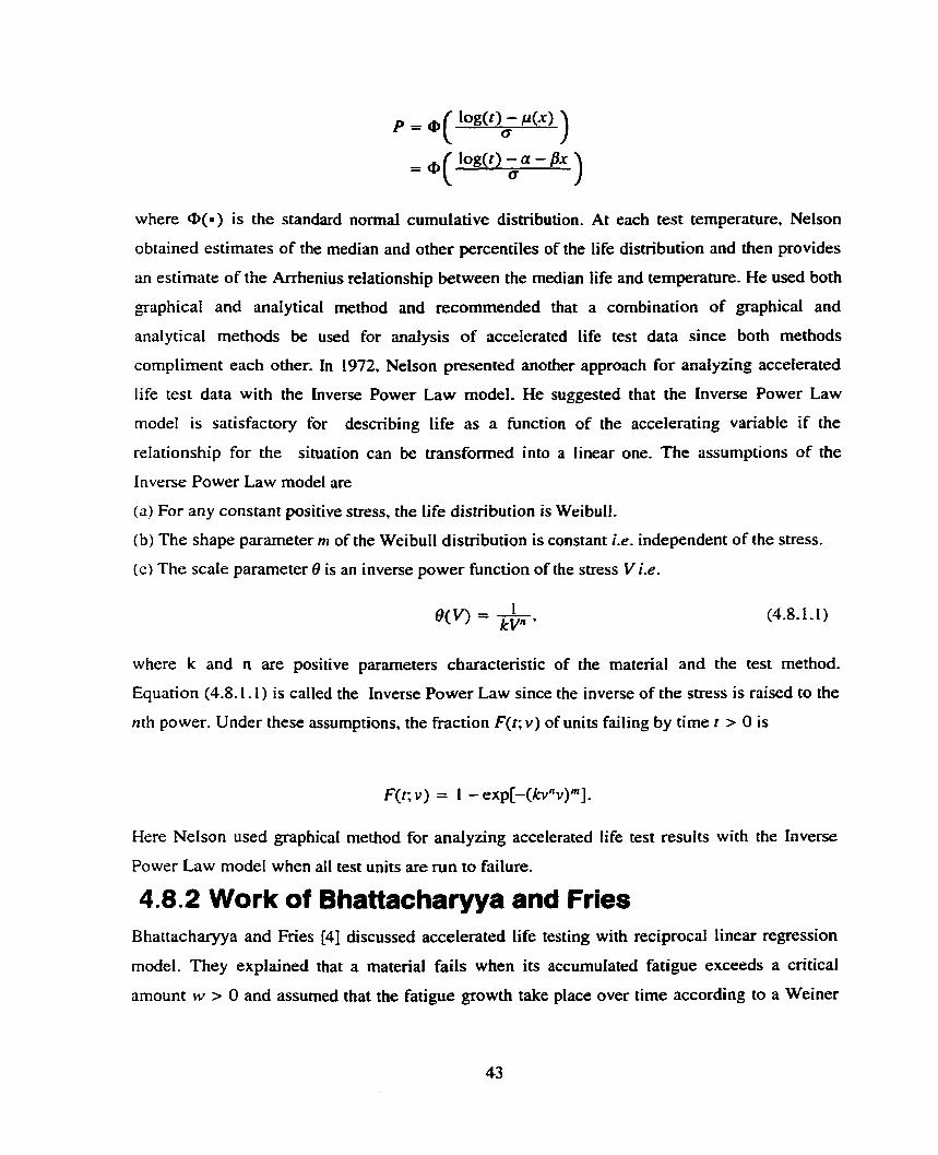
where @(a ) is the standard normal cumulative distribution. At each test temperature, Nelson

obtained estimates of the median and other percentiles of the life distribution and then provides

an estimate of the Arrhenius relationship between the median Iife and temperature. He used both

graphical and analytical method and recommended that a combination of graphical and

analytical methods be used for analysis of accelerated life test data since both methods

compliment each other. in 1972, Nelson presented another approach for a n a i m g acceierated

life test data with the Inverse Power Law model. He suggested that the Inverse Power Law

model is satisfactory for describing Iife as a hinction of the accelerating vari-able if the

rehtionship for the situation can be transfonned into a linear one. The assumptions of the

Inverse Power Law model are

(a) For any constant positive stress, the life dismbution is Weibull.

(b) The shape parameter m of the Weibull distribution is constant Le. independent of the stress.

( c ) The scale parameter O is an inverse power function of the stress V i.e.

where k and n are positive parameters characteristic of the material and the test method.

Equation (4.8.1.1) is called the Inverse Power Law since the inverse of the stress is raised to the

nth power. Under these assumptions, the fraction F(t; v) of units failing by time t > O is

Here NeIson used graphicaI method for anaiyzing accelerated life test results with the Inverse

Power Law model when al1 test units are run to failure.

4.8.2 Work of Bhattacharyya and Fries Bhattacharyya and Fries [4] discussed accelerated Iife testing with reciprocal linear regression

model. They explained that a material fails when its accumulated fatigue exceeds a critical

amount w > O and assumed that the fatigue growth take place over time according to a Weiner

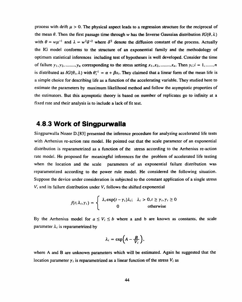
process with drift p > O. The physical aspect leads to a regression structure for the reciprocal of

the mean 8. Then the first passage time through BV has the Inverse Gaussian distribution IG(8, A)

with û = wp-' and A = w26-Z where l j2 denote the diffusion constant of the process. Actually

the IG model conforms to the structure of an exponential famiIy and the methodoIogy of

optimum statistical inferences including test of hypotheses is well developed. Consider the time

of failure y 1 ,y2, ...-....,y, corresponding to the stress settïng x~ ,x2, ...... ..,x,. Then Yi; i = 1, .--..-. n

is distributed as 1G(Bi, l) with OfL = a + Px. They claimed that a linear form of the mean life is

a simple choice for describing life as a function of the accelerating variable. They studied here to

estimate the parameters by maximum likelihood method and follow the asymptotic properties of

the estimators. But this asymptotic theory is based on number of replicates go to infinity at a

fixed rate and their analysis is to include a lack of fit test.

4.8.3 Work of Singpurwalla Singpurwalla Nozer D.[83] presented the inference procedure for analyzing accelerated life tests

with Arrhenius re-action rate model. He pointed out that the scale parameter of an exponential

distribution is reparametrized as a function of the stress according to the Arrhenius re-action

rate model. He proposed for meanina@l inferences for the problem of accelerated life testing

when the location and the scale parameters of an exponential failure distribution was

reparametrized according to the power nile model. He considered the following situation.

Suppose the device under consideration is subjected to the constant application of a single stress

V, and its failure distribution under Vi follows the shifted exponential

By the Arrhenius model for a 5 Vi ( b where a and b are known as constants, the scale

parameter Li is reparametrized by

where A and B are unknown parameten which will be estimated. Again he suggested that the

location parameter yi is reparametrized as a linear function of the stress V; as

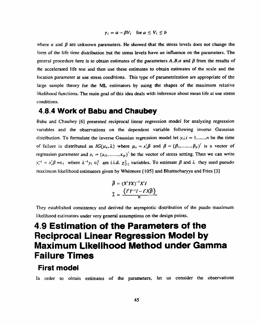
where a and /3 are unknown parameters, He showed that the stress levels does not change the

form of the Iife time distribution but the stress levels have an influence on the parameters, The

general procedure here is to obtain estimates of the parameters A,B,a and P fiom the results of

the accelerated life test and then use these estimates to obtain estimates of the scale and the

location parameter at use stress conditions. This type o f parametrïzation are appropriate of the

large sample theory for the ML estimators by using the shapes of the maximum relative

likelihood functions. The main goal of this idea deals with inference about mean life at use stress

conditions.

4.8.4 Work Babu and Chaubey

variables and the

of Babu [63 presented

observations

and Chaubey reciprocal linear regression model for analyzing regression

on the dependent variable following inverse Gaussian

distribution. T o formulate the inverse Gaussian regression model let yi;i = 1, ....., n be the time

of failure is distrïbuted as IG(p,. A.) where px = xjp and P = (Pi. ---...J3,,)' is a vector of

regression parameter and ri = (x i l , ........ x,)' be the vector of stress setting. Then we can wnte

y;' = x : p +Ei where A-'yi E: are i.i.d. x : ~ , variables. T o estimate /3 and L they used pseudo

maximum likelihood estimators given by Whitmore [ 1 OS] and Bhattacharyya and F i e s [3]

They established consistency and derived the asymptotic distribution of the psudo maximum

Iikelihood estimators under very general assumptions on the design points.

4.9 Estimation of the Parameters of the Reciprocal Linear Regression Model by Maximum Likelihood Method under Gamma Failure Times First model In order to obtain estimates of the parameters, let us consider the observations

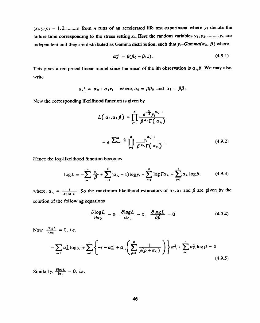
(x, ,yi); i = 1,2. ........ n frorn n runs of an accelerated life test expriment where y, denote the

failure time corresponding to the stress setting xi. Here the random variables y 1. y2, .........y, are

independent and they are disaibuted as Gamma distribution, such that yi-Gamm(a,. P ) where

This gives a reciprocal linear mode1 since the mean of the ith observation is a,#. We may also

write

Now the corresponding likelihood function is given by

Hence the log-likelihood function becomes

where, a,, = ' . So the maximum likelihood estimators of ao,a, and /3 are given by the do+ a 1x1

solution of the following equations

2logL Now - = O, i.e. dao

n n

xi& + C x&, log /? = O i-1

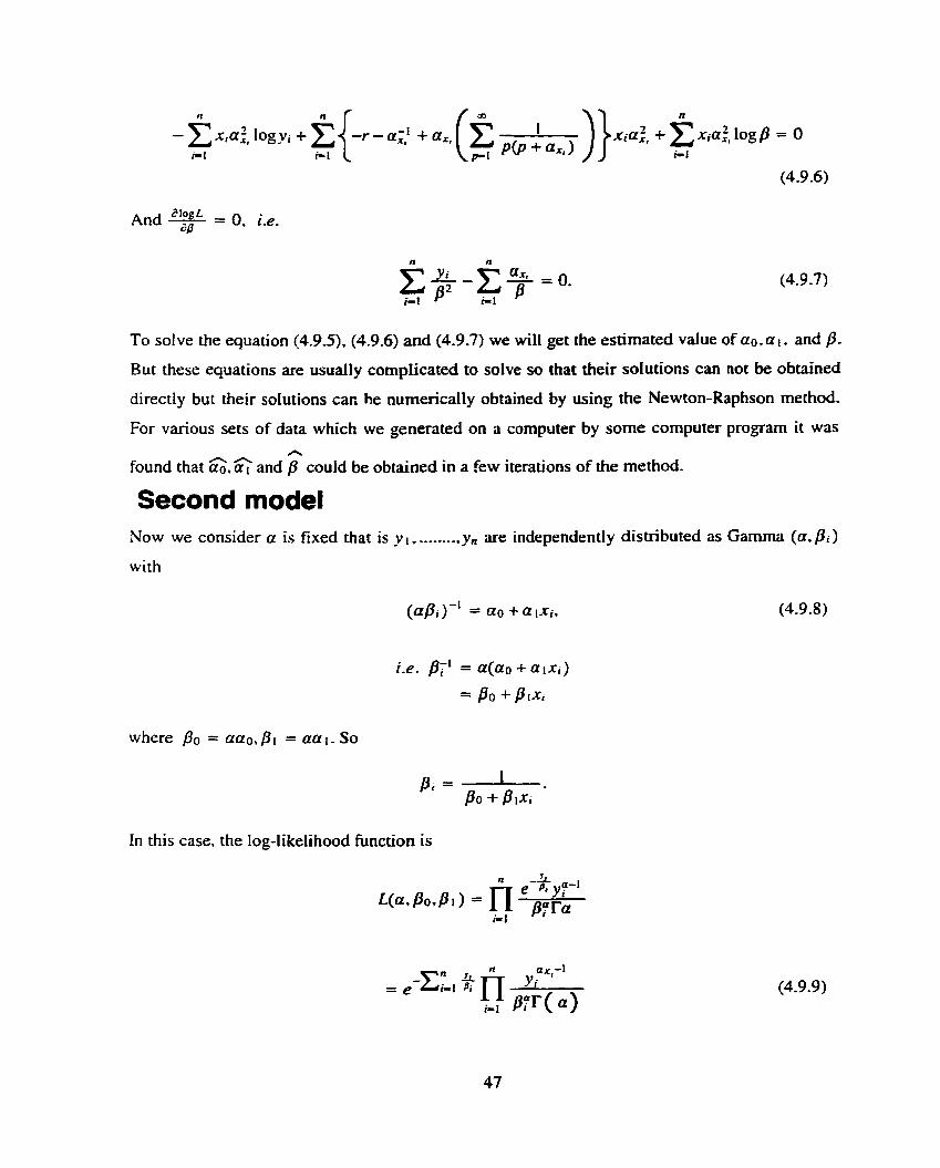
(4.9.6)

Elo L And -$- = O. Le.

To solve the equation (4.9 5). (4.9.6) and (4.9.7) we will get the estimated value of ao. a 1. and p. But these equations are usually complicated to solve so that their solutions can not be obtained

directfy but their solutions can he nurnericdly obtained by using the Newton-Raphson method.

For various sets of data which we generated on a computer by some computer program it was A

A A found that ao, a l and P could be obtained in a few iterations of the method.

Second model Now we consider a is fixed that is yl, .........y, are independently distributed as Gamma (a&)

with

where 00 = uao,Pl = au[ - So

Pi = I

BO + Pixi *

In this case, the log-likelihood function is

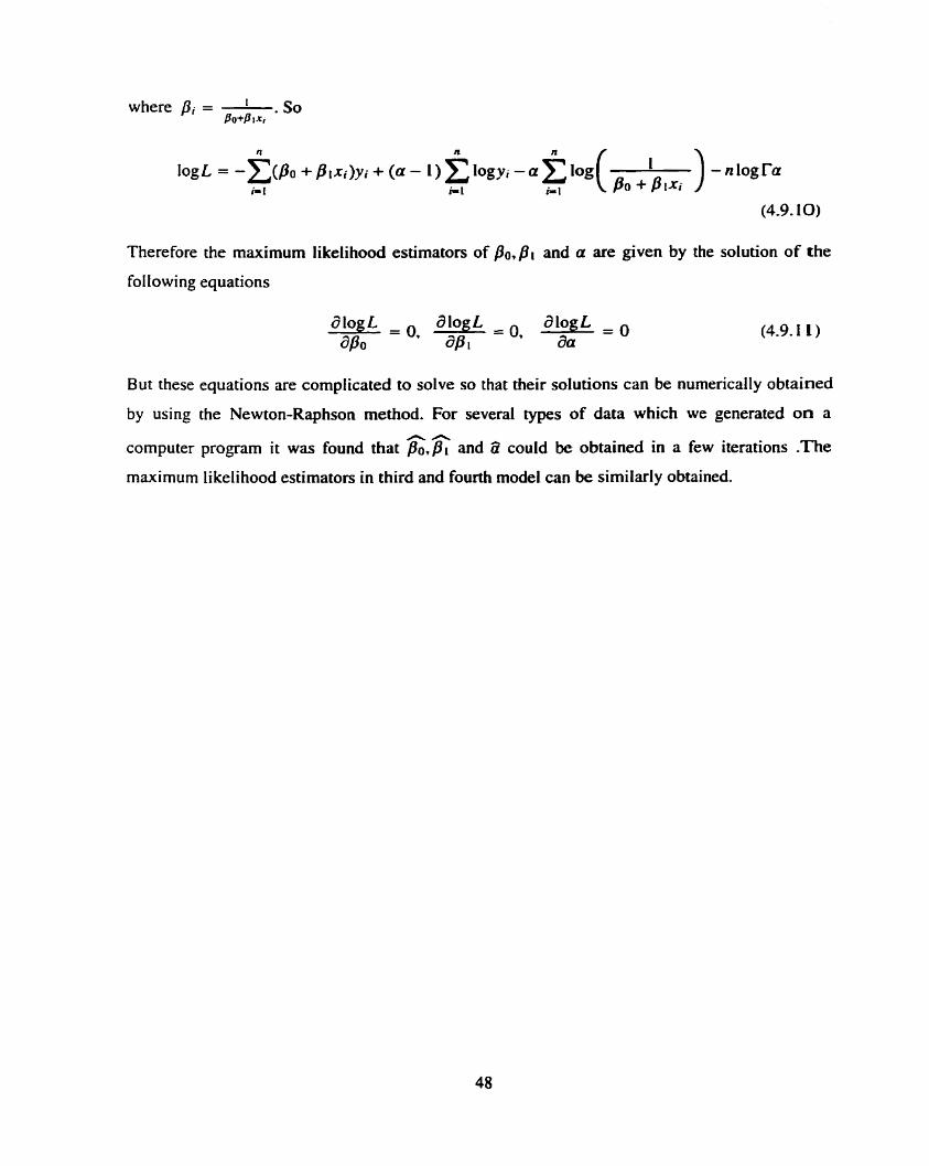
where pi = - . So Po+P 11,

Therefore the maximum Iikelihood estimators of po.pi and a are given by the solution of the

following equations

But these equations are complicated to solve so that their solutions can be numerically obtained

by using the Newton-Raphson method. For several types of data which we generated on a A-

computer prognm it was Found that povBl and û could be obtained in a few iterations .The

maximum likelihood estimators in third and fourth mode1 can be similarly obtained.

5 Numerical Illustration 5.1 Data

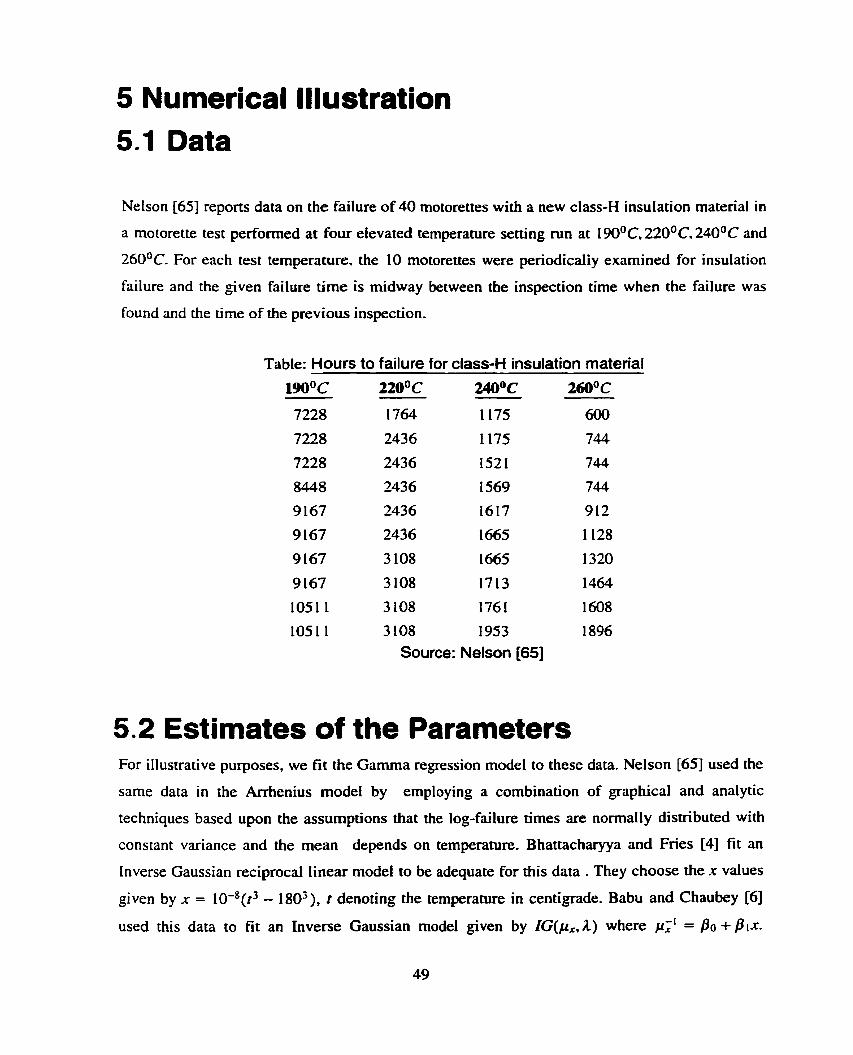
Nelson [65] reports data on the failure of 40 motorettes with a new class-H insulation material in

a motorette test perfonned at four elevated temperature setting mn at 190°C. 22U°C. 240°C and

260°C. For each test temperature. the 10 motorettes were perïodicaliy examined for insulation

failure and the given failure time is midway between the inspection tirne when the failure was

found and the time of the previous inspection.

Table: Hours to failure for class-H insulation material

lW°C 220°C 24Q°C 260°C

7228 1764 1175 600

7228 2436 1175 744

7228 2436 1521 744

8448 2436 1569 744

9 167 2436 1617 912

9 167 2436 1665 1128

9 167 3 108 1665 1320

9 167 3 108 17 13 1464

1051 1 3 108 176 1 1608

105 1 1 3 108 1953 1896 Source: Nelson [65]

5.2 Estimates of the Parameters For illustrative purposes, we fit the Gamma regression model to these data. Nelson [6S] used the

same data in the Arrhenius model by employing a combination of graphical and analytic

techniques based upon the assumpùons that the log-failure times are normally disnibuted with

constant variance and the mean depends on temperature. Bhattacharyya and F i e s [4] fit an

Inverse Gaussian reciprocal linear model to be adequate for this data . They choose the x values

given by n = 10-8(t3 - 1 803), t denoting the temperature in centigrade. Babu and Chaubey 161

used this data to fit an Inverse Gaussian model given by IG(p,,A) where piL = P a +pi*-

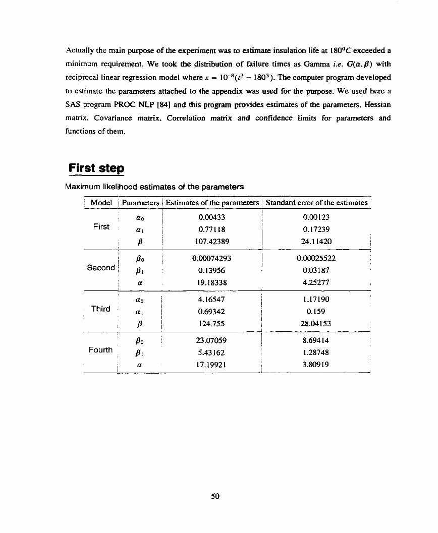
Actually the main purpose of the expriment was to estimate insulation life at 1 80°C exceeded a

minimum requirement. We took the distribution of failure times as Gamma Le. G(a,P) with

reciprocal linear regression mode1 where x = 1 0 - ~ ( t ~ - 1803). The computer program developed

to estimate the parameters attached to the appendix was used for the purpose, We used here a

SAS program PROC NLP 1841 and this program provides estimates of the parameters, Hessian

matrix, Covariance matrix, Correlation matrix and confidence limits for parameters and

functions of them.

First step Maximum likelihood estimates of the parameters

Mode1 i Parameten ) Estirnates of the parameters / Standard error of the estimates ' I

ao i 0.00433 l 0.00 123 I First

1

a1 l

i 0.77 1 18 1 O. 17239 1

P 1 107.42389 1 24.1 1420 I

l

i Po 1 1 Second ; p , 1

- -

1 CIO 4.16547 l

1

1.17190 1

Third I

I ! 1

0-69342 1 O. 159 p i 124.755 i I 28.04153

i I

I

I

Po 23 .O7059 I ? 8 -694 14

Fourth 1

P I 5.43 162 I 1.28748 , a ! 17.19921 I I I 1 3.809 19

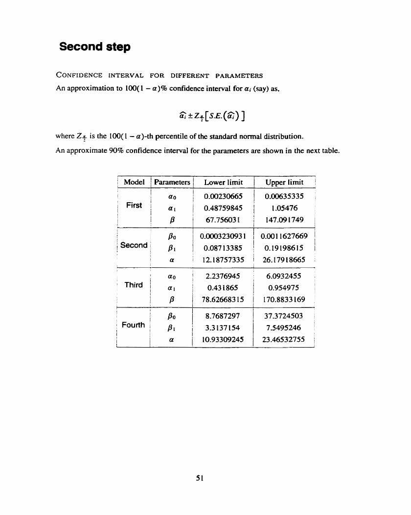
Second step

CONFIDENCE INTERVAL FOR DIFFERENT PARAMETERS

An approximation to 100u - a)% confidence interval for ai (say) as.

G & Z+ [S.E. (G) ]

where Z+ is the 100( 1 - a)-th percentile of the standard normal distribution.

An approximate 908 confidence interval for the parameters are shown in the next table.

I

2

ao 2.2376945 6.0932455 I

1 Third I 1 / 0.43 1865 1 0.954975

j 1 p 1 78.62668315 170.8833169 t 1

PO j 8.7687297 i 37.3724503 I ! Fourth 1 pi

l ! 1 3.3137154 1 7.5495246

! 1 a j 10.93309245 23.46532755 i 1

Mode1 / Parameten 1 Lower limit 1 Upper limit i

I ' 0.00230665 0.00635335 I a0 1 !

: First a 1 0.48759845 1

I 1 1.05476 / 1 !

1 L j p !

1 1

67.75603 1 i 147.091749 1

i 1 /?O I 1 0.000323093 1 / 0.00 1 1627669 I 1 i S e c o n d 1 1 0.08713385 0.19198615 1

I I CI ; 12.18757335 26.179 18665

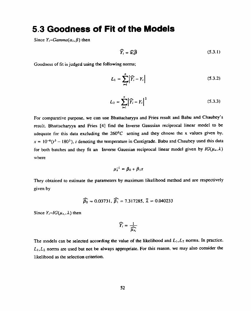
5.3 Goodness of Fit of the Models Si nce Y,-Gamma(ai, P ) then

Goodness of fit is judged using the following noms;

For comparative purpose, we can use Bhattacharyya and Frïes result and Babu and Chaubey's

result. Bhattacharyya and Fnes 141 find the Inverse Gaussian reciprocal linear model to be

adequate for this data excluding the 260°C setting and they choose the x values given by.

x = 10-8(t3 - 1803), r denoting the temperature in Centigrade. Babu and Chaubey used this data

for both batches and they fit an Inverse Gaussian reciprocal linear model given by IG(px. A )

w here

They obtained to estimate the parameters by maximum likelihood method and are respectively

given by

Since Yi-IG(p,, . A.) then

The models can be selected according the value of the likelihood and Li ,L2 norms. In practice.

Li, L2 noms are used but not be always appropriate. For this reason. we may also consider the

likeli hood as the selection criterion.

The table below shows the L i . Lz noms and log likelihood function in the different mode1

i Model 1 Log likelihood 1 ! First 1 19068.23003 1 18 101706.78 1 306.1948749

i Third / 1965 1.03725 1 19547356.6 1 ! 309.2575996 i

: Babu and Chaubey / 18784.80094 1 1823 1932.08 [ ; - I

5.4 Conclusions and further Research For the Gamma farnily, it can be observed that the reciprocai regression model for scale

parametrization gives the better result than other types of model according to Li norm. but first

model. Le. shape pararnetrization is better according to Lz norrn. Thus we consider the

likelihood criterion according to which the first model is the best. Note also that the estimators

given in Babu and Chaubey [dl provide best model amongst al1 the models considered according

ro the Li nom this property is lost when we consider L2 norm.

For funher research, we can consider the use of the family of power transformations of

dependent variable before carrying out the regression analysis. Below we give some more details

of this.

Let YI, - - -, Y, be a random sample fiom some non-normal density function. Let u s assume

that they follow a gamma distribution. Consider the folIowing transformation

where Y= ( Y 1 . - - -. Y,)' and fiA) = (fi), O - . , YIL))' . Here EL) is the transformed value of Y; - - for some Â= (2-1 , . - -, &) from the W l y A = ( A i , - - , Âk) of transformation. From the above - transformation we assume that Y<"' - Gamm(nA, PA). We will use the method of maximum

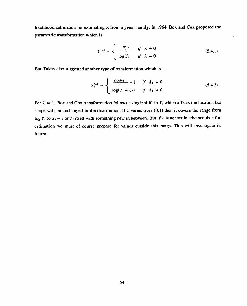
Iikelihood estimation for estimating

pararnetric transformation which is

A nom a given family. In 1964. Box and Cox proposed the

But Tukey also suggested another type of transformation which is

For A = 1. Box and Cox transformation follows a single shifi in Yi which affects the location but

shape will be unchanged in the distribution. If A varies over (O. 1 ) then it coven the range from

log Yi to Y, - 1 or Yi itself with something new in between. But if A is not set in advance then for

estimation we must of course prepare for values outside this range. This will investigate in

future.

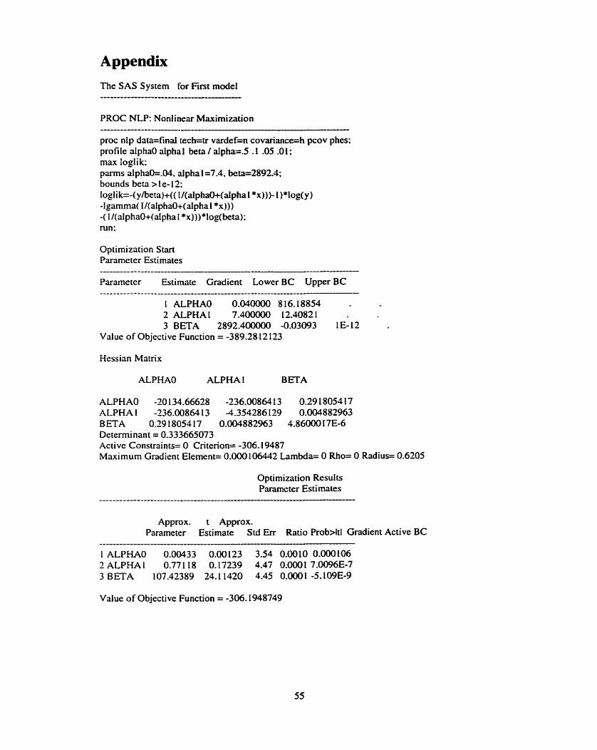
Appendix The SAS S ystem for First mode1

PROC NLP: Nonlinear Maximization

proc nlp data=finai tech=tr vardef=n covariance=h pcov phes; profile alpha0 alpha1 beta / alpha=S -1 -05 -01: m a Ioglik: p m s alpha0=.04. alpha 1 =7.4, beta=2892.4; bounds beta >le- 12: logli k=-( y/beta)+(( I/(aiphaO+(aipha 1 *x)))- 1 ) *Iog(y ) -]gamma( l/(alphaO+(alphal *x))) -( 1 /(alphaO+(atphal *x)))*log(beta): mn;

Optirnization Start Parameter Estimates ---------------------------- Parameter Estimate Gradient Lower BC Upper BC -------------------------------- --

1 ALPH A0 0.040000 8 16.18854 2 ALPHA 1 7.400000 12.4082 1 3 BETA 2892.400000 -0.03093 1 E-12

Value of Objective Function = -389.28 12 123

Hessian Matrix

ALPHA0 ALPHAI BETA

ALPHAO -20 1 34.66628 -236.00864 t 3 0.29 180% 17 ALPHA 1 -236.00864 13 -4.354286 129 0.004882963 BETA 0.29 180% 17 0.004882963 4.86000 17E-6 Determinant = 0.333665073 Active Consuaints= O Criterion= -306.19487 Maximum Gradient €lement= 0.000 IO6442 Lambda= O Rho= O Radius= 0.6205

Optimization Results Panmeter Estimates

Approx. t Approx. Parameter Estimate Std Err Ratio Prob>ltl Gradient Active BC

----------------------- ---- 1 ALPHAO 0.00433 0.00123 3.54 0.0010 0.000106 2 ALPHA 1 0.77 1 18 0.17239 4.47 0.000 1 7.0096E-7 3 BETA 107.42389 24.1 1420 4.45 0.0001 -5.109E-9

Value of Objective Function = -306.1948749

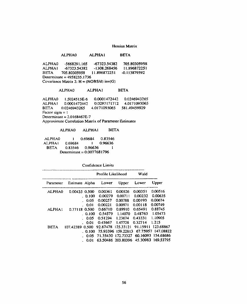
Hessian Matrix

ALPHA0 ALPHA 1 BETA

ALPHAO -566829 1.165 -6732354382 705.80305958 ALPHA 1 -67323.54382 - 1308.268456 1 1.89687225 f BETA 705.80305958 1 1 -89687225 1 -0.1 13879592 Determinant = 4958235.1736 Covariance Matrix 2: H = (NOBSfd) inv(G)

ALPHA0 ALPHA 1 BETA

ALPHAO 1 50245 1 5E-6 0.000 1472442 0.0246943265 ALPHA 1 0.000 1472442 0.0297 17 17 12 4.0 17 1093065 B ETA 0.0236943265 4.0 17 1093065 58 1 -49459929 Factor sigm = 1 Determinant = 2.0 168467E-7 Approximate Correlation Mavix of Parameter Estimates

ALPHA0 ALPHA1 B ETA

ALPHA0 1 0.69684 0.83546 ALPHA 1 0-69684 1 0.96636

BETA 0.83546 0.96636 1 Determinant = 0.007768 1796

Confidence Limits ----------------------------------

Profile Likelihood Wald ..................... ------------- -

Parrimeter Estimate Alpha Lower Upper Lower Upper ---------------- ------------ ----

ALPHAO 0.00433 0500 0.0036 1 0.00526 O.OO3S 1 0.005 16 . O. 100 0.00279 0.007 1 1 0.00232 0.00635 . 0.05 0.00257 0.00788 0.00193 0.00674

0.01 0.00221 0.00971 0.001 18 0.00749 ALPHA 1 0.77 1 18 0.500 0.667 10 0.899 10 0.6549 1 0.88745

. O. 100 0.54579 1,14070 0.48763 1.05473

. 0.05 0.5 1294 1.23674 0.4333 1 1.10905 - 0.01 0.45667 1.45726 0.327 14 1.215

BETA 107.42389 0.500 92.87478 125.33 12 1 9 1.159 1 1 123.68867 . O. 100 75.93396 159.228 13 67.75957 147.08822 . 0.05 7 1.35430 172.73327 60.16093 154.68686 . 0.0 1 03.50486 203.80396 45.30983 169.53795

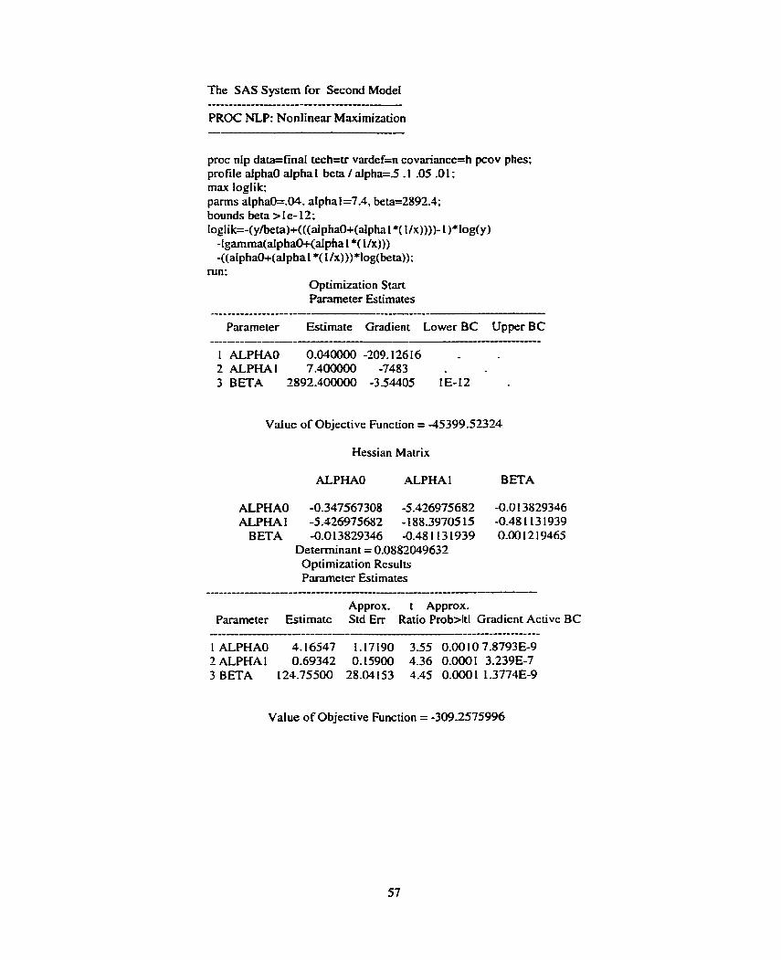
The SAS System for Second Modet ------------- PROC NLP: Nonlinear Maximization

proc ni p data=final tech=u vardef=n covariance=h pcov phes; profile alpha0 aiphaI beta / alpha=5 -1 -05 -01; max loglik; parms alpha0=.04, alpha t =7.4, beta=2892.4; bounds beta > f e- 12; Ioglik=-(y/beta)+(((aiphaO+(alp ha l *( l/x))))- l )*log(y )

-1gamrna(alphaO+(alpha 1 *( l/x))) -((alphaû+(alphal *( l/x)))*log(beta));

run; Optimization S m Parme ter Estimates

----------A--

Parameter Esùmate Gradient LowerBC UpperBC

1 ALPHAO 0.040000 -209.I2616 2 ALPHA1 7.400000 -7483 3 BETA 2892.400000 -3.54405 LE-12

Vaiue of Objective Function = -45399.52324

Hessian Matrix

ALPHA0 ALPHA 1 BETA

ALPHAO -0.347567308 -5.426975682 -0.0 13829346 ALPHA 1 -5.426975682 - 188.39705 15 -0.48 1 13 1939

BETA -0.0 13829346 -0.48 1 13 1939 0.00 12 19465 Determinant = 0.0882049632 Optimization Results Parameter Estimates

---------------------------p--P---

Approx. t Approx. Parameter Estimate S td Err Ratio Pro b>ltl Gradient Active BC

1 ALPHAO 4.16547 1.17 190 3.55 0.00 10 7.8793E-9 2 ALPHA 1 0.69342 O.lS9OO 4.36 0.000 1 3.239E-7 3 BETA 124.75500 28.04153 4.45 0.0001 1.3774E-9

Value of Objective Function = -309.2575996

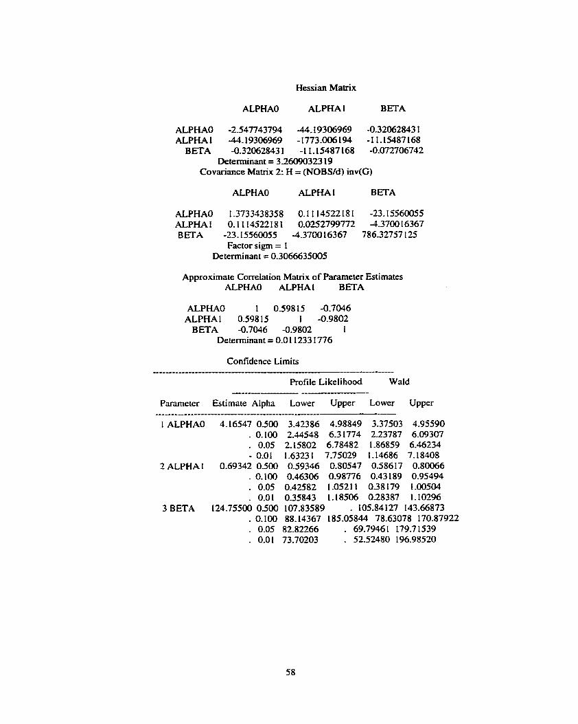
Hessian Matnx

ALPHA0 ALPHA 1 BETA

ALPHAO -2.547743794 -44,19306969 -0.32062843 1 ALPHA 1 -44.19306969 - 1773-006 194 - 1 1.15487 168

BETA -0.32062843 1 -1 1.15487 168 -0.072706742 Determinant = 3.26090323 19

Covariance Matrix 2: H = (NOBS/d) inv(G)

ALPHA0 ALPHA1 BETA

ALPHAO 1.3733338358 0.1 1 14522 18 1 -23.15560055 ALPHA f O. 1 f 14522 1 8 1 0.0252799772 -4.3700 1 6367 BETA -23.15560055 -4.3700 16367 786.32757 125

Factor sigm = 1 Determinant = 0.3066635005

Approxirnate Correlation Mavix o f Parameter Estirnates ALPHA0 ALPHA1 BETA

ALPHA0 1 0.59815 -0.7046 ALPHA1 0.598 15 1 -0.9802

BETA -0.7046 -0.9802 I Determinant = 0.0 1 1233 1776

Parameter Gtimate Alpha Lower Upper Lower Upper -A------------------ -----

1 ALPHAO

2 ALPHA 1

3 BETA

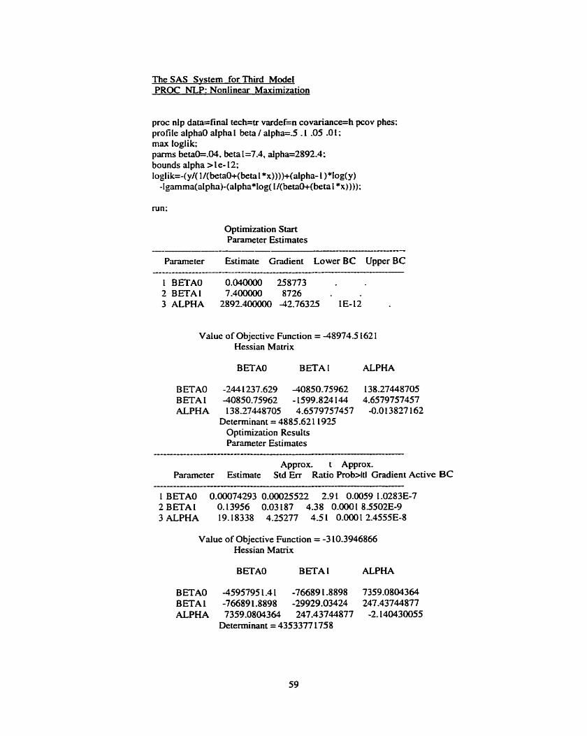
The SAS Svstem forThird Mode1 PROC NLP: Nonlinezu Maximization

proc nlp data=final tech=u varde f=n covariance=h pcov phes: profile alpha0 alpha 1 beta / alpha=J -1 .OS .O 1 ; rnax toglik; parrns betak.04, beta l=7.4, alpha=2892.4; bounds alpha > le-12: loglik=-(y/( l/(betaO+(beta 1 *x))))+(alpha- 1 )*log( y)

-Igamma(alpha)-(alphaw( l/(betaO+(beta 1 *x))));

Optirnization Start Parameter Estimates

Parmeter Estimate Gradient Lower BC Upper BC

1 BETAO 0.040000 258773 2 BETAl 7.400000 8726 3 ALPHA 2892.400000 -42,76325 1E-12

Value of Objective Function = -48974.5 162 1 Hessian Matrix

BETAO BETA 1 ALPHA

BETAO -244 1237.629 -40850.75962 138.27448705 BETA 1 -40850.75962 - 1599.824 144 4.6579757457 fCPHA 138.27448705 4.6579757457 -0.0 13827 162

Deteminant = 4885.621 1925 Optimization Results Parameter Estimates

Approx. t Approx. Parameter Estimate Std Err Ratio Prob>ltl Gradient Active BC

- 1 BETAO 0.00074293 0.00025522 2.9 1 0.0059 1 -0283E-7 2 BETAI O. 13956 0.03187 4.38 0.0001 85502E-9 3 ALPHA 19.18338 4.35277 4.5 I 0.000 1 2.4555E-8

Vaiue of Objective Function = -3 10.3946866 Hessian Mauix

BETAO BETA 1 ALPHA

BETAO -4595795 1.4 1 -76689 1.8898 7359.0804364 BETA 1 -76689 1.8898 -29929.03424 247.43744877 ALPHA 7359.0804364 247.43744877 -2.140430055

Determinant = 4353377 1758

Covariance Matrix 2: H = (NOBS/d) inv(G)

BETAO BETAI ALPHA

BETAO 6 5 138242E-8 4- 12 17 1 13E-6 0.0007004309 BETAI 4.1217113E-6 0.0010156188 0.1315782877 ALPHA 0.00070043~ O. 13 15782877 18.086049033

Factor sigrn = 1 Determinant = 2.297067E-11

Approximate CorreIation Matrix of Pararneter Estimates

BETAO BETAl ALPHA

BETAO f 0.50675 0.64532 BETA1 0.50675 1 0.97083 ALPHA 0.64532 0,97084 1

Determinant = 0.0 19 198321

Confidence Limits

Profile Likelihood Wald --- -

Pararneter Estimate Alpha Lower Upper Lower Upper

1 BETAÛ 0.0007429 0.500 0.00058 16 0.0009223 0.0005708 0.0009 15 1 . O. 100 O.OOO369 1 0.00 12 1 O.ûûO323 1 0.00 1 16

0.05 0.0003068 0.001 3 1 0.0002427 3.001 24 . 0.01 0.0001929 0.00153 0.0000855 O.OOI40

2 B ETA 1 0.13956 0500 0.1 1953 0.16202 0.1 1807 0.16 1 O6 . 0.100 0.09339 0,19855 0.08714 0.19198 . 0.05 0.08593 0.21 144 0.07710 0.20202 - 0.0 1 0.07242 0.23809 0.05747 0.22 165

3ALPHA 19.1838 0.500 . 16,31493 22.05182 - 0.100 . 27.05488 12.188 19 26.17856 . 0.05 12.026 1 1 28.77568 10.848 10 27.5 1 865 - 0.01 . 33.33 1 12 8.22897 30.13778

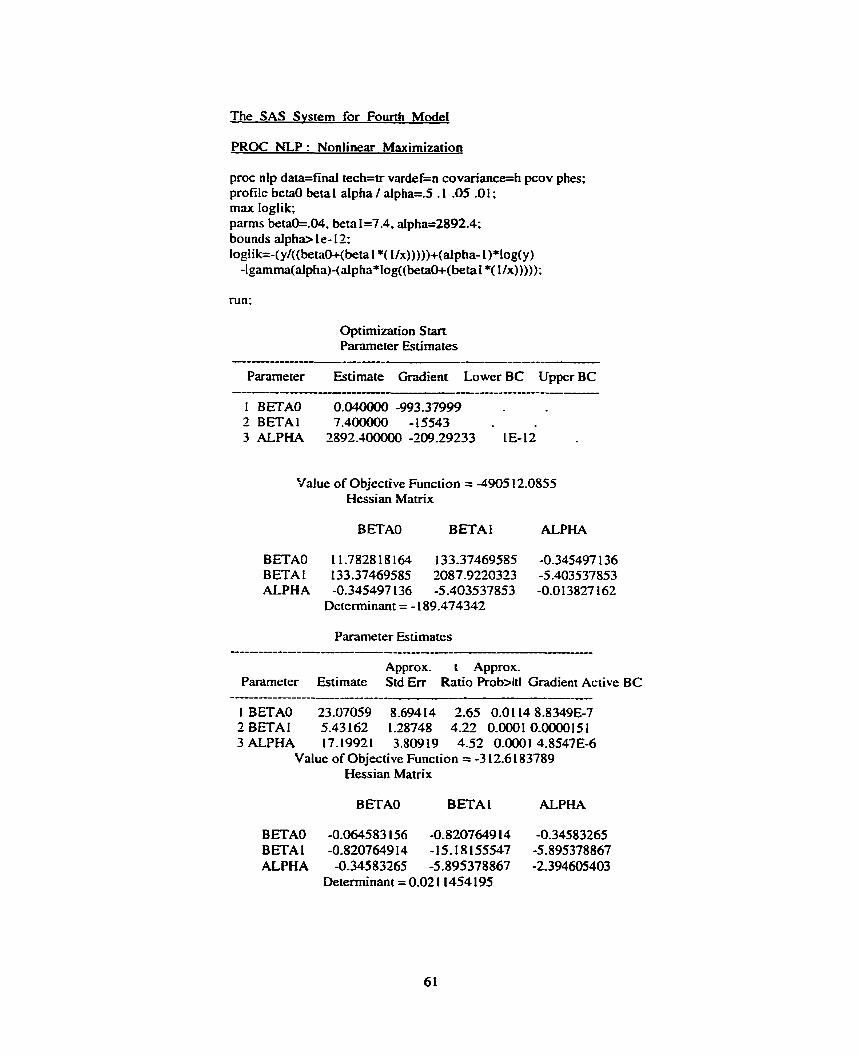
The SAS Svstem for Fourth Mode1

PROC NLP : Nonlinear Maximization

proc nlp data=final tech=tr vardef=n covariance=h pcov phes; profile betaO betal alpha / alpha=5 -1 -05 -01: max loglik; parms betaO=.W, bewI=7-4, aIpha=2892.4; bounds alpha> le- 12: loglik=-(yl((bemW(betal*( t/x)))))+(alpha- I)*log(y) -lgamma(alpha)-(dpha*log((bemo+(beta 1 *( Ilx))))):

run:

Optirnization Seart Panmeter Estimates

Parameter Estimate Gradient Lower BC Upper BC

I B ETAO 0.040000 -993.37999 2 BETAl 7 ,400000 - 1 5543 3 ALPHA 2892.3000 -209.29233 LE- 13

Value of Objective Function = -4905 12.0855 Hessian Matrix

BETAO BETA 1 ALPHA

BETAO 1 1.7828 18 164 133.37469585 -0.345497 136 BETA t 133,37469585 2087.9220323 -5.403537853 ALPHA -0.345497 136 -5.403537853 -0.0 13827 162

Deteminant = - 189.474342

Panmeter Estimates ----------------PA-- -

Approx. t Approx, Parameter Estimate Std Err Ratio Prob>ltl Gradient Active BC

1 BETAO 23.07059 8.694 14 2.65 0.01 14 8.8349E-7 2BETAl 5.43162 1.28748 4-22 0.000I0.0000151 3 ALPHA 17.19921 3.80919 452 0.0001 4.8547E-6

Value of Objective Function = -3 12-6 183789 Hessian Mauix

BETAO BETAI ALPHA

BETAO -0.064583 156 -0.8207649 14 -0.34583265 BETA 1 -0.8207649 14 - 15-18 155547 -5,895378867 ALPHA -0.34583265 -5.895378867 -2.394605403

Determinant = 0.02 1 1454 195

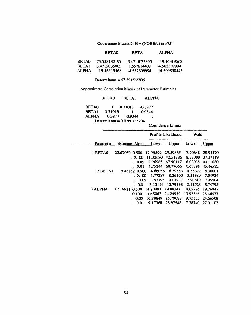
Covariance Matnx 2: H = (NOBS/d) inv(G)

BETAO BETA 1 ALPHA

BETAO 75588 132197 3.47 15036805 -19-463 19568 BETA 1 3.47 15036805 1.6576 14408 -4.582309994 ALPHA - 19.463 19568 -4582309994 14509890345

Determinant = 47.29 1565895

Approximate Correlation Mavix of Parameter Estimates

BETAO BETAI ALPHA

BETAO 1 0-3 1013 -05877 BETA1 0.31013 t -0.9344 ALPHA -0.5877 -0.9344 1

Determinant = 0-0260 125204 Confidence Limits

- - - - - - - - -

Profile LikeIihood Wald -

Pmmeter Estimate Abha Lower U w e r Lower lluper

1 BETAO 23.07059 0.500 17.95599 29.59865 . O, 100 1 1.32680 425 1886 . 0.05 9.26985 47.901 17 . 0.01 4.75244 60.77066

2 BETAI 5.43 162 0.500 4.66056 6.39553 . O. 100 3.77287 8.26100 . 0.05 3.53795 9.01937 . 0.01 3.13114 10.79198

3 ALPHA 17.1992 1 0.500 14.80493 19.8834 1 . O. 100 1 1.68067 24.24959 . 0.05 10.78849 25.79088 . 0.01 9.17368 28.97543

Bibliography

Aroian, L. A, A study of Fisher's z distribution, Annals of Mathematical Statistics, 12, pp 429-

448, 1939.

Ahrens. L.H., The lognormal distribution of the elernents, Geochimica et Cosmochimica Acta, 6.

pp 121-131, 1954,

Bhattacharyya, G. K. and Fries, A., On the Inverse Gaussian multiple regression and mode1

checking procedures, Elsevier Science Publishers B.V. (North HoIland), Editor Basu, AP.. pp

87- 100. 1986.

Bhattacharyya, G, Kmd Fries, A., inverse Gaussian regression and accelerated life tests.

Mathematical Statistics, Hayward, California, pp 101-1 18, 1982a.

Bhattacharyya, G. K. and Fries, A., Fatigue failure models Birnbaum Saunders VS. Inverse

Gaussian, IEEE Transactions on retiability,Vol.R-3 t , NOS, pp 439-441, 1982-

Babu, GJ. and Chaubey, Y.P., Asyrnptotics and Bootstnp for Inverse Gaussian regression,

Ann.Inst.Statist.Math, Vo1.48, No. 1, pp 75-88, 1996.

Beirlant, J.. Goegebeur, Y., Verlaak, R. and Vynckier, P., Burr Regression and Portfolio

segmentation. ELSEVIER Science B.V. Insurance: Mathematics and Econornics 23, pp 23 1-250,

1998.

Bagdonavicius,V. and Nikulin, M-, Semi paramecric models in accelerated life testing, Queen's

papers in Pure and Applied Mathematics, Kingston, Ontario, Canada, No-98, 1995.

Bagdonavicius, V. and Nikulin, M., Additive and Multiplicative serniparametric models in

accelerated Iife testing and Survival analysis, Queen's papers in Pure and Applied Mathematics,

Kingston, Ontario.Canada, Vol. 108, 1998.

Banarjee, A. K. and Bhattacharyya G. K., A purchase Incidence Mode1 With inverse Guassian

bterpurchase Times, Journal of Americal Statist. Association, 7 1, pp 823-829, 1976.

Bana jee , A. er al.. Bayesian results for the IG distribution with application, Technometrics, 2 1,

pp 823-829, 1983.

[12] Bachelier. L,, Theorie de la speculation, Ann- Sci- Ec. Nom. Super, 17, pp 21-86, 1900. the

Barton, D.E.. The Probability distribution fitnction of a mm of squares, Trabajos de Estadistica,

4, pp 199-207, 1953.

Bliss. CI., The method of Probits, Science, 79, pp 38-39, 1934-

Cramer, H., Mathematical methods of Statistics, Princeton University press, Princeton. 1946.

Cramer, J.S., Econometrïc applications of maximum likelihood methods, Cambridge University

press, Cambridge, London, 1986.

Cochran. W-G., Some difficulties in the statisticai anaiysis of replicated experiments- Empire

Journal of Experimental Agriculture, 6, pp 157-163, 1938.

Chayes, F.. The lognormal distribution of the elements: a discussion, Geochimica et

Cosmochimica Acta, 6, pp 1 19- 120, 1954.

Chhikara, R.S. and Folks, J.L.. The IG distribution as a life time model. Technometrics, 19, pp

46 1-468, 1974.

Chhikara, R.S. and Folks, J.L., Optimum test procedures for the mean of first passage time

distribution in Brownian motion with positive drift, Technometrics, 18, pp 189-193, 1976.

Cuniss. J.H.. On transformations used in the andysis of variance, Annals of Mathematical

Statistics, 14, pp 107-122, 1943.

Chhikara, R- et al. Prediction lirnit for the IG distribution, Techno. 2 1 pp 3 19-324. 1982-

Draper, N.R, and Smith, H., Applied regression Analysis, John Wiley and Sons Inc. New York.

1966.

Dhrymes, P.J., On devising unbiased estimators for the parameters of the Cobb-Douglas

production function, Econometrica, 30, pp 297-304, 1962.

Das. S C . , The fitting of truncated type ïil curves to daiiy rainfall data, Austraiian Journal of

Physics, 7, pp 298-304, :955.

126 Dabrowska, DM., and Doksum, KA., Partial likelihood in Transformations Models with

Censored Data, Scand. J. Statist., 15, pp 1-23, 1988.

Dugue, D. Application des properties de la Iimit au sens du calcul des probabilities a I'tude des

diverses question d'estimation, J.Ecol. Poly., 3, No. 4,305, 1937-

Eaton. W.W. and Whitmore, G.A., Length of stay as a stochastic process: a general approach and

application to hospitalization for schizophrema. J. Math. Social, 5. pp 273-292, 1977-

Ferrel, E-B., Control charts for log normal universes, Industrial Quaiity Control, 15. No.2, pp 4-

6. 1958.

Gallant, A-R., Nonlinear Statistical models, John Wiley and Sons, NewYork ,1978-

Giordano. A.A. and Hsu, F.M., Least square estimation with applications to digital signal

processing, John Wiley and Sons, New York, 1962.

Goon, A.M.. Gupta, M.K. and Dasgupta, B., An outline of Statistical theory (Volume-2). The

World press private Iirnited, Culcutta, India, 1987.

Gupta, S C . and Kapoor,V.K., Fundamentals of Mathematical Statistics, Sultan Chand and Sons.

Daryaganj. New Delhi- 1 10002, 1970.

Greene,W.H., Econornetrics analysis. Second edition, Maxwell Macmillan international

hblishing Group, New York, 1993.

Galton, F.. The geometnc mean in vital and social statistics, Proceeding of the Royal Society of

London, 29. pp 365-367, 1879.

Gaddum, J.H., Reorts on biological standards, II: Methods of biological assay depending on a

quantal response, special Report series, Medical research council, London, No. 183, 1933.

Goba, F.A., Bibliography on Thermal Aging of Electrical Insulation, IEEE,Trans. on Electrical

insulation, EI-4, pp 3 1-58, 1969.

Gibrat, R., Les Inegalites Economiques, Paris: Libraire du Recueil Sirey, 193 1.

Gibrat, R., Une doi des repartitions, t'effect proportionned, Bulletin de statistique, General,

France, 19,469ff, 1930.

[JO] Gmndy, P.M., The expected frequencies in a sample of an animai population in which the

abundances of species are log normally distributed, Part- 1, Biometrika, 3.8, pp 427-434. 195 1 -

[4 1 ] Grestein, G. et al., Random walk modek for the spike activity of a neuron. Biophys. Jour., 4.pp

41-68, 1964.

[QI Heyde, CC., On a property of the lognormal distribution, Journal of the Royal Statistical Society,

Senes B, 25, pp 392-393, 1963

Hennanson, R.E. and Johnson, HP., Generaiîzed flood- frequency relationship, Iowa state

Journal of Science. 41, pp 247-268, 1967.

Herdan, G.. The relation between the dictionary distribution and the occurance distribution of

word Iength and its importance for the study of quantitative lingustics, Biometrika 45, pp 222-

228, 1958.

Herdan, G., The advanced theory of language as choice and chance, New York, Spnnger, 1966.

Huzurbazar. V.S.. The likelihood equation. consistency and maxima of the likelihood function.

Ann. Eugen. London, 14. 185, 1948.

Johnson,N.L. and Kotz,S.. Continuous univariate distributions-1, John Wiley and Sons, New

York ,1970

Johnson, R.C.E. and Johnson, N.L., Survival models and data analysis, John Wiley and Sons.

New York, 1980.

Kotz, S. and Neumann, J., On distribution of precipitation arnounts for the periods of increasing

length, Journal of geophysical research, 68,pp 3635-364 1. Addendum: 69,800-80 1. 1963-

Khamis. S.H., Incomplete Gamma function expansions of Statistical distribution functions,

Bulletin of the International Statistical institute, 37, pp 385-396, 1960.

Kalbfleisch, J.D. and Prentice, R.L., The Statisticai Analysis of faiiure time data, John Wiiey and

Sons, New York, 1980.

Kapur, J.N. and Saxena, H.C., Mathematical Statistics, S-Chand and Company Ltd. Ramnagar,

New Delhi- 1 1 O O S , India, 198 1.

Kolmogorov, AN., Uber das logarithmisch normale verteilungs gesetzder Teilchen bei

Zerstuckelung, Doklady Akademii Nauk, SSSR, 3 1, pp 99-10 1, 1941.

Kartashov, G.D., Methods of Forced (Augmented) experiments (in Russian), Znaniye Press,

Moscow, 1979.

Koopmans, L-H- Owen, O.B. and Rosen blatt, IL, Confidence intervals for the coefficient of

variation for the normal and lognormal dist"., Biometrika 51, pp25-32, 1964.

Lehmann, E.L., Testing Statistical Hypothesis, John Wiley and Sons, New York, 1986.

Lawless, J.F.. Statistical Models and Methods for Life tirne Data, John Wiley and Sons.. New

York. 1982.

Lancaster, A., Stochastic mode1 for the duration of a strïke, J. Roy. Statist. Soc. ser. A., 135, pp

357-37 1, 1973

Mensah. R.D.. Some aspects of survival analysis, M.Sc. thesis. Concordia University, Montreal,

Quebec. Canada, 198 1.

Miner, M.A., Cumulative Damages in Fatigue, Journal of Applies Mechanics, 12, pp AI59-

A164, 1945.

Miller, R.L. and Goldberg, E.D., The normal distribution in geochernistry, Geoc himica et

Cosmochimica Acta, 8, pp 53-62, 1955.

Morrison, J.. The lognomal distribution in quality control, Applied Statistics. 7, pp 160-172,

1958.

Marcus, Allan H., Some exact dist". in t d k noise theory, Adv. in appl. probab., 7, pp 593-606,

1975,

Neter, J., Wasserrnan,W., Kutuer, M.H, Applied linear Statistical Models, IRWIN, Home Wood,

iL60430, Boston, MA02 1 16, 1971.

Nelson, W., Accelerated testing, Statistical rnodels, Test plans and Data analysis, John Wiley and

Sons, New York, 1990.

Nelson, W., Applied life data analysis, John Wiley and Sons, New York, 198 1.

Nelson, W., Analysis of accelerated life test data, Part-l : The Arrhenius model and Graphical

methods, IEEE Transactions on electrical insulation, VolXI-6, No-4, pp 165- 18 1, 197 1.

Nelson, W., Andysis of accelerated life test data- Part-2: Numerical methods and test planning,

E E E Transactions on eIectrical insulation, Vol.EI-7, pp 36-55, 1972.

Nelson. W., Andysis of accelerated life test data- Part-3: Product cornparisons and checks on the

validity of the mode1 and data, IEEE Transactions on electricai insulation, Vol-EI-7, pp 99-1 19.

1973.

Nelson. W.. Graphical analysis of accelerated life test data with the Inverse Power Law model,

IEEE transactions on reliability, VOIX-2 1, No, 1, pp 2- 1 1, 1972.

Nelson, W., A survey of rnethods for planning and anaiyzing accelerated tests. IEEE transactions

on electrical insulation Vol-EI-9, No. 1, pp i 2- 18, 1974-

Oldham, P.D., On estimating the arithmatic means of lognormally distributed populations,

Biometrics, 2 1. pp 235-239, 1965.

Pearson. K. (Ed.), Tables of the Incomplete gamma function, London: H.N. stationary office.

(since 1934. Cambridge University Press), 1922.

Pearson, K. (Ed.), On a criterion that a given system of deviations from the probable in the case

of correlated systern of variables is such that it can be resonably supposed to have a risen from

random sampling, Philosophical Magazine, 5th series, 50, pp 157- 175, 1900.

Pearce. S C . . Lognormal distn., Nature, London, 156, pp 747. 1945.

Prohorov, Yu. V ., On the Lognormal distn. in geo-chemistry, Teonya Veroyatnostie iee

Primeneniya, 10, pp 184-187, 1963.

Rao, CR.. Linear Statistical inference and its applications, Second edition, Wiley Eastern

limited, New Delhi, india, 1984.

Rohn, W.B., Reliability prediction for complex systems, proceedings of the 5th National

Symposium on Reliability and Quality Control in Electronics, pp 38 1-388, 1959.

Sedyakin, N.M., On one physical principle in reliability theory, Techn., Cybemetics, 3, pp 80-

87, 1966.

Stuart. A. and Ord, J-K-, Kendall's Advanced theory of Statistics. Volume-2, Oxford University

press, New York, 199 1.

Sprott, D.A. and Kalbfleisch, J.D., Examples of likelihoods and cornparision with point estimates

and large sarnple approximations, American Statistical Association Journal, pp 468-484, 1969.

Shenton. L.R. and Bowman, K.O., Maximum likelihood estimation in small samples, Charles

Griffin and Company Ltd. London and High Wycombe, 1977-

SingpurwalIa. N.D.. Inference from accelerated life tests using Arrhenius type re-

parametrizations, Technometrics, Vol. 15, No2, pp 289-299, 1972.

SASIOR Technical Report: The NLP Procedure, SAS Instinite inc., SAS Campus Drive. Cary,

NC 275 13, USA, 1997.

Schrodinger. E., Zur Theorie der Fall-und steigversuche an Teilchenn mit Brownscher

Bewegung, physikalische zeitschrift, 16, pp 289-295, 19 15.

Tarikere, N.N., Inverse Gaussian distribution and analysis of factorial experiments, M-Sc- thesis,

Concordia University, Montreal, Quebec, Canada, 199 1.

Tweedie. M.C.K., Statistical properties of Inverse Gaussian distribution. Annals of Mathematical

Statistics, 28, pp 362-377, 1957.

Tomlinson, R.C., A simple sequential procedure to test whether average conditions achieve a

certain standard, Applied Statistics, 6, pp 198-207, 1957.

Tiku, M-L., Estirnating the parameters of lognomal distribution from censored samples,

Journals of the American Statistical Association, 63 pp 134-140, 1968.

Tiku, M.L. Approxirnating the general non-normal variance ratio sampling distribution,

Biometrika, 5 1, pp 83-95, 1964.

Tiku, M.L.. Laguerre series forms fo non-central chi-square and F-distributions, B iometrika, 52.

pp 4 15-427, 1964.

Uven, M.J. Van, Logarithrnic frequency distribution, proceeding of the Royal Academy of

Science, Amsterdam, 19, pp 533-546, 19 17,

Uven. M.J. Van, Skew frequency curves, Proceeding of the Royal Academy of Science,

Amsterdam. 19, pp 670-684. 19 17.

Wicksell, S.D., On the genetic theory of frequency Arkiv for Mathe-matik, Astronomi och Fysik

12, pp 1-56, 1917.

Wise. M.E.. Tracer dilution curves in cardiology and random walk and log-normal distribution.

Acta Physiologica Pharmacologica Neerlandica, 14, pp 1 ïS-2W. 1966.

Williams, C.B., The use of logarithrns in the interpretation of certain entomological problems,

Annals of Applied Biology, 24, pp 404414.1937.

Williams. C.B., A note on the statistical andysis of sentence length, Biometrika. 3 1, pp 356- 36 1.

1940.

Wu, Chuan-yi, The types of limit distributions for some ternis of variational series, Scientia

Sinica, 15, pp 749-763. 1966,

Wald, A., Sequential Analysis, John Wiley and Sons-, New York, 1947-

Wasan, M.T. and Roy, L.K., Tables of inverse Gaussian probabilities, Annais of Mathematical

Statistics. 38, pp 299, 1967.

Welech, B.L., The significance of the difference between two means when the popdation

variances are unequal, Biometrika. 29, pp 350-36 1. 1938-

Wasan, M.T., First passage time dist. of Brownian motion, Monograph, Dept. of Mathernatics.

Queen's University, Kingston, Ontario, 1968.

Weiss, G., Random walks and their applications, Amer- Scientist., 7 1, pp 65-7 1, 1983-

Whitmore, G.A., An IG mode1 for labour turnover, J.R. Statist. Soc. senes A, 142(A), pp 468-

479, 1979.

Whitmore, G.A.. A regression method For censored inverse gaussian data, Canada, J. Statist., 1 1.

pp 305- 315, 1983.

[ 1061 Yurkowsky, W.. Schafer, R E and Finkelstein, IM.. Accelerated Testing Technology, Rome Air

Development center Tech. Rep. RADC-TR-67420, Gnffiss AFB, W., 1967.