ABSTRACT

Title of Document: MOLYBDENUM ISOTOPE SYSTEMATICS

IN NATURAL AND EXPERIMENTAL SETTINGS

Kathleen Dwyer Scheiderich, Ph.D. 2010 Directed By: Professor Richard J. Walker, Department of

Geology Molybdenum isotopes have a broad potential applicability for

paleoenvironmental analysis, particularly with respect to questions of

eutrophication history, development of anoxia, and sedimentation under

conditions of varying oxygenation. Using a double-spike method, the Mo

isotope proxy was applied to sediments and water samples from the

Chesapeake Bay, where the severity of seasonal anoxic episodes has been

increasing over the last century. It was discovered that isotopic fractionation is

occurring in the estuary, as indicated by the large differences between the

δ98Mo of Mo dissolved in the water and authigenic Mo in the sediments.

Increased variability of δ98Mo values and increased authigenic Mo deposition

were likely related to the onset of coastal anoxic episodes in the Bay.

Sediment samples from the Eastern Mediterranean were also analyzed for

δ98Mo, along with redox-sensitive element concentrations (Re, Mo, V, Ba, and

Fe). Over the past 5 million years, climatic shifts have driven cyclic

oceanographic changes in the Mediterranean, specifically basin-wide anoxic

episodes, which are visible in the sedimentary sequence as layers that are

highly enriched in redox-sensitive elements and organic matter (sapropels). I

investigated whether δ98Mo values, in conjunction with other proxies, could be

used to infer the degree to which the deep basin was affected by anoxic

conditions, and how this may have changed between individual anoxic

episodes. There were clear temporal differences in the apparent severity of

anoxia in the Mediterranean, as reflected by the proxies in the sapropels. The

amount of Mo in Mediterranean seawater did not change during sapropel

deposition, and therefore, the basin likely remained open to circulation. I

collaborated in a project to determine whether Mo isotopes could be

fractionated at high temperature and pressure in an experimental system,

designed to mimic natural hydrothermal-type porphyry systems. It was found

that Mo isotopes are fractionated between a melt and vapor phase under the

experimental conditions, and in a manner consistent with equilibrium

exchange processes. Molybdenum entering the melt phase undergoes a

coordination change to higher coordination number, thus preferentially

enriching the vapor phase in the heavier Mo isotopes.

MOLYBDENUM ISOTOPE SYSTEMATICS IN NATURAL AND EXPERIMENTAL SETTINGS

By

Kathleen D. Scheiderich

Dissertation submitted to the Faculty of the Graduate School of the University of Maryland, College Park, in partial fulfillment

of the requirements for the degree of Doctor of Philosophy

2010 Advisory Committee: Professor Richard J. Walker, Chair Professor Emeritus George R. Helz Associate Professor James Farquhar Associate Professor Michael Evans Dean's Representative Professor Russell Dickerson

© Copyright by Kathleen Dwyer Scheiderich

2010

ii

Dedication

For Mom and Dad and Hobbes.

iii

Acknowledgements

I would not have been able to finish the project without the assistance of

Aaron Pietruszka and Jasper Konter, who collaborated in developing the

double spike. Many thanks to the Maryland Department of Natural Resources

for water samples, the Maryland Geological Survey and Elizabeth Canuel

(VIMS) for sediment samples for the Chesapeake Bay project. The Ocean

Drilling Program is gratefully acknowledged for providing the samples for the

Mediterranean project. I thank Michael Mengason, who entertained a crazy

idea and set up the experiments that are described in Chapter 5. Aubrey

Zerkle taught me about sulfur isotopes, and also got me involved with

analyzing Mo isotopes in nitrogen-fixing organisms. Richard Ash and Bill

McDonough have always been ready to help with analytical questions and

have been great about all aspects of the struggle with the Nu. Jen Obernier

provided me with timely life advice and general lifting of spirits. Rich and

George have been excellent mentors, and I hope to live up to their high

standards.

iv

Table of Contents Dedication ....................................................................................................... ii Acknowledgements ........................................................................................ iii Table of Contents ........................................................................................... iv List of Tables ................................................................................................. vii List of Figures ................................................................................................ viii Chapter 1: Molybdenum: An Introduction ........................................................ 1

The Basics ................................................................................................... 1 Molybdenum geochemistry in water and sediments .................................... 5

Summary ................................................................................................ 11 Molybdenum isotopes ................................................................................ 12 The contributions of this work .................................................................... 20

Chapter 2: Method development at UMD ...................................................... 22 First attempts ............................................................................................. 22 Brief overview of MC-ICP-MS .................................................................... 23 Mass bias and instrumental fractionation ................................................... 25 Methods for fractionation correction ........................................................... 29

Sample-standard bracketing ................................................................... 29 External fractionation correction ............................................................. 29 Double-spiking ........................................................................................ 30 Attempts with SSB and external FC ....................................................... 35 Preparation and Calibration of a 97Mo-100Mo Double Spike................. 42 Long term result for standards with the double spike method ................ 52

Column chemistry and sample preparation ................................................ 57 Column Chemistry .................................................................................. 57 Sediment sample preparation ................................................................. 63 Preparation of water samples ................................................................. 63

Chapter 3: Century-long record of Mo isotopic composition in sediments of a seasonally anoxic estuary (Chesapeake Bay) ............................................... 66

Abstract ...................................................................................................... 66 Introduction ................................................................................................ 67 Sample descriptions ................................................................................... 69

Water samples ....................................................................................... 69 Sediment samples .................................................................................. 72

Methods ..................................................................................................... 78 Sample preparation and measurement .................................................. 78 Calculation of authigenic Mo .................................................................. 80

Results ....................................................................................................... 81 Chesapeake Bay and Susquehanna River water ................................... 81 Chesapeake Bay and Susquehanna River sediments ........................... 84

Discussion.................................................................................................. 88 Authigenic Mo formation in the Chesapeake Bay ................................... 88 Molybdenum isotope fractionation in Chesapeake Bay sediments ......... 93

v

Isotopic mass balance in the Chesapeake Bay watershed..................... 96 Conclusions ............................................................................................... 97

Chapter 4: Molybdenum isotopic signatures in Pliocene-Pleistocene aged Mediterranean sapropels ............................................................................... 99

Abstract ...................................................................................................... 99 Introduction .............................................................................................. 100 Background .............................................................................................. 104

Mediterranean hydrography ................................................................. 104 Tectonics .............................................................................................. 105 Messinian Salinity Crisis ....................................................................... 105

Site Description ........................................................................................ 106 Age model ............................................................................................ 108 Sampling strategy ................................................................................. 109 High temporal resolution sampling across a single sapropel (S25) ...... 111 Low temporal resolution samples ......................................................... 111

Analytical Methods ................................................................................... 112 Results ..................................................................................................... 115

Results in S25 ...................................................................................... 125 Results in the sediments between 1.48 and 1.90 Ma ........................... 126

Discussion................................................................................................ 127 Redox-sensitive element concentrations .............................................. 129 Fe/Al in Mediterranean sediments ........................................................ 130 δ98Mo of Mediterranean sediments ...................................................... 130 Variable Mo sources ............................................................................. 133 Variable Mo fractionation mechanisms ................................................. 136 Sulfur isotope systematics in 969D ...................................................... 142 Molybdenum in hemipelagic sediments ................................................ 148 Rhenium/Molybenum ratios .................................................................. 151

Conclusions ............................................................................................. 156 Chapter 5: Experimental determination of Mo isotope fractionation at high temperature and pressure ........................................................................... 158

Abstract .................................................................................................... 158 Introduction .............................................................................................. 158 Experimental Methods ............................................................................. 162 Results ..................................................................................................... 164

Calculation of α (vapor-melt) and DMo (vapor-melt) .............................. 167 Discussion................................................................................................ 167

Possible problems ................................................................................ 167 Interpretation of experimental results ................................................... 170

Geological implications ............................................................................ 176 Conclusions ................................................................................................. 178 Appendices .................................................................................................. 181

Appendix 1. Supplemental information to Chapter 3. ............................... 181 Appendix 2. Supplemental information to Chapter 4 ................................ 184

Core photos .......................................................................................... 184 Duplicate Samples ............................................................................... 187

vi

Sample preparation for sulfur isotope analysis ..................................... 187 Mass balance calculations .................................................................... 188

Bibliography ................................................................................................. 193

vii

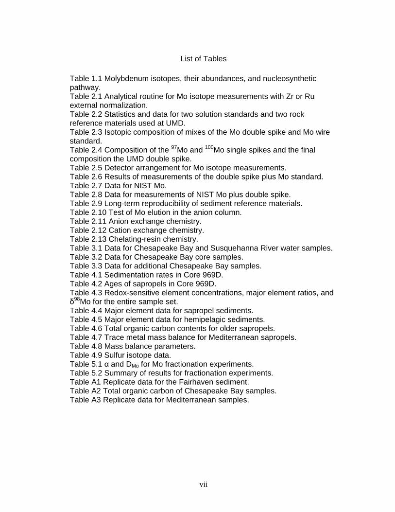
List of Tables Table 1.1 Molybdenum isotopes, their abundances, and nucleosynthetic pathway. Table 2.1 Analytical routine for Mo isotope measurements with Zr or Ru external normalization. Table 2.2 Statistics and data for two solution standards and two rock reference materials used at UMD. Table 2.3 Isotopic composition of mixes of the Mo double spike and Mo wire standard. Table 2.4 Composition of the 97Mo and 100Mo single spikes and the final composition the UMD double spike. Table 2.5 Detector arrangement for Mo isotope measurements. Table 2.6 Results of measurements of the double spike plus Mo standard. Table 2.7 Data for NIST Mo. Table 2.8 Data for measurements of NIST Mo plus double spike. Table 2.9 Long-term reproducibility of sediment reference materials. Table 2.10 Test of Mo elution in the anion column. Table 2.11 Anion exchange chemistry. Table 2.12 Cation exchange chemistry. Table 2.13 Chelating-resin chemistry. Table 3.1 Data for Chesapeake Bay and Susquehanna River water samples. Table 3.2 Data for Chesapeake Bay core samples. Table 3.3 Data for additional Chesapeake Bay samples. Table 4.1 Sedimentation rates in Core 969D. Table 4.2 Ages of sapropels in Core 969D. Table 4.3 Redox-sensitive element concentrations, major element ratios, and δ98Mo for the entire sample set. Table 4.4 Major element data for sapropel sediments. Table 4.5 Major element data for hemipelagic sediments. Table 4.6 Total organic carbon contents for older sapropels. Table 4.7 Trace metal mass balance for Mediterranean sapropels. Table 4.8 Mass balance parameters. Table 4.9 Sulfur isotope data. Table 5.1 α and DMo for Mo fractionation experiments. Table 5.2 Summary of results for fractionation experiments. Table A1 Replicate data for the Fairhaven sediment. Table A2 Total organic carbon of Chesapeake Bay samples. Table A3 Replicate data for Mediterranean samples.

viii

List of Figures

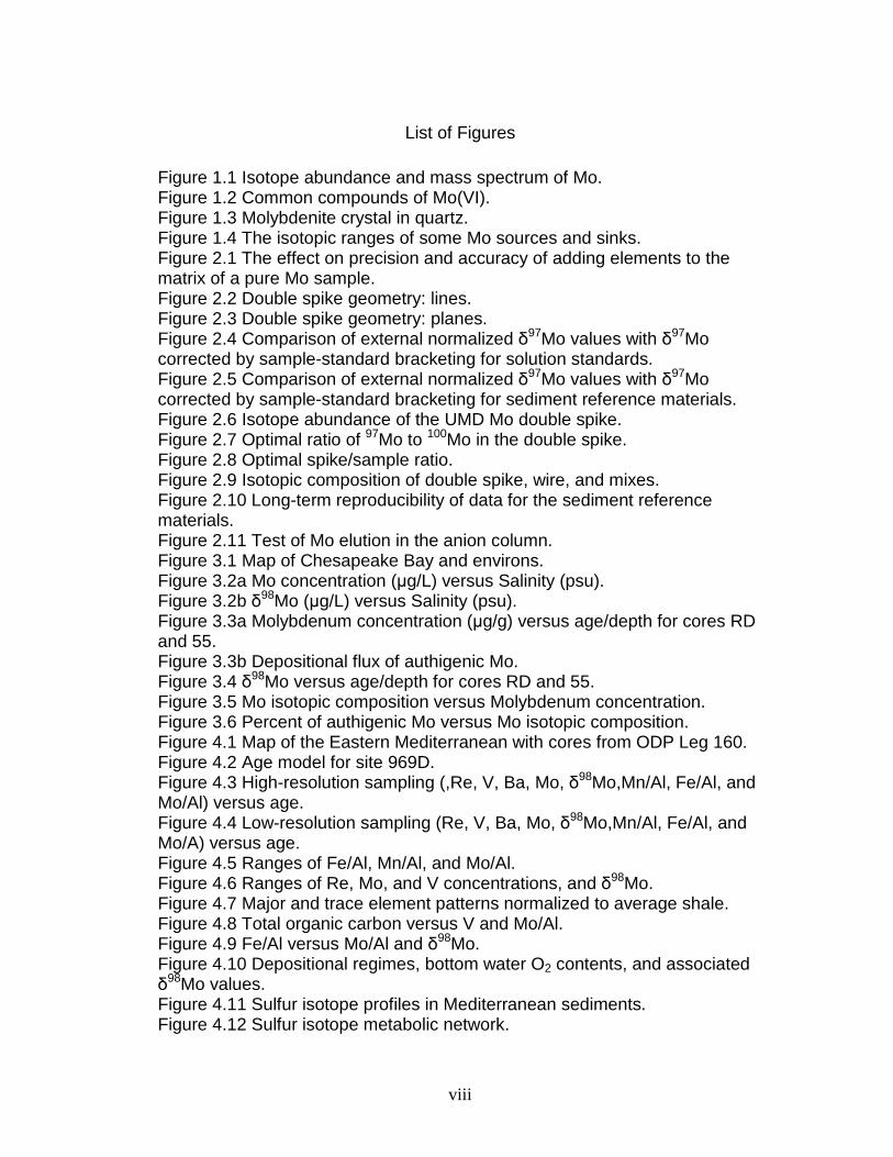
Figure 1.1 Isotope abundance and mass spectrum of Mo. Figure 1.2 Common compounds of Mo(VI). Figure 1.3 Molybdenite crystal in quartz. Figure 1.4 The isotopic ranges of some Mo sources and sinks. Figure 2.1 The effect on precision and accuracy of adding elements to the matrix of a pure Mo sample. Figure 2.2 Double spike geometry: lines. Figure 2.3 Double spike geometry: planes. Figure 2.4 Comparison of external normalized δ97Mo values with δ97Mo corrected by sample-standard bracketing for solution standards. Figure 2.5 Comparison of external normalized δ97Mo values with δ97Mo corrected by sample-standard bracketing for sediment reference materials. Figure 2.6 Isotope abundance of the UMD Mo double spike. Figure 2.7 Optimal ratio of 97Mo to 100Mo in the double spike. Figure 2.8 Optimal spike/sample ratio. Figure 2.9 Isotopic composition of double spike, wire, and mixes. Figure 2.10 Long-term reproducibility of data for the sediment reference materials. Figure 2.11 Test of Mo elution in the anion column. Figure 3.1 Map of Chesapeake Bay and environs. Figure 3.2a Mo concentration (µg/L) versus Salinity (psu). Figure 3.2b δ98Mo (µg/L) versus Salinity (psu). Figure 3.3a Molybdenum concentration (µg/g) versus age/depth for cores RD and 55. Figure 3.3b Depositional flux of authigenic Mo. Figure 3.4 δ98Mo versus age/depth for cores RD and 55. Figure 3.5 Mo isotopic composition versus Molybdenum concentration. Figure 3.6 Percent of authigenic Mo versus Mo isotopic composition. Figure 4.1 Map of the Eastern Mediterranean with cores from ODP Leg 160. Figure 4.2 Age model for site 969D. Figure 4.3 High-resolution sampling (,Re, V, Ba, Mo, δ98Mo,Mn/Al, Fe/Al, and Mo/Al) versus age. Figure 4.4 Low-resolution sampling (Re, V, Ba, Mo, δ98Mo,Mn/Al, Fe/Al, and Mo/A) versus age. Figure 4.5 Ranges of Fe/Al, Mn/Al, and Mo/Al. Figure 4.6 Ranges of Re, Mo, and V concentrations, and δ98Mo. Figure 4.7 Major and trace element patterns normalized to average shale. Figure 4.8 Total organic carbon versus V and Mo/Al. Figure 4.9 Fe/Al versus Mo/Al and δ98Mo. Figure 4.10 Depositional regimes, bottom water O2 contents, and associated δ98Mo values. Figure 4.11 Sulfur isotope profiles in Mediterranean sediments. Figure 4.12 Sulfur isotope metabolic network.

ix

Figure 4.13 Correlation between Mo and δ34S. Figure 4.14 Rhenium/Molybdenum ratios. Figure 4.15 Rhenium concentration versus δ98Mo. Figure 5.1 δ98Mo and Mo quantities in run products. Figure 5.2 α and DMo with respect to run duration. Figure 5.3 Fugitive Mo in the experiments. Figure 5.4 Run duration versus Mo concentration. Figure 5.5 δ98Mo versus Mo concentration in run products. Figure A1 Core photo of 969D 4H. Figure A2 Core photo of 969D 5H. Figure A3 Isotope mixing model for the Nile river. Figure A4 Ternary diagram of potential trace metal sources.

1

Chapter 1: Molybdenum: An Introduction

The Basics Molybdenum is a highly refractory, moderately siderophile, group VIB

transition metal with seven stable isotopes (Fig. 1.1, Table 1.1). These seven

isotopes are produced by various nucleosynthetic processes (p, r, and s, Table

1.1). In common with many transition metals, Mo can occur in a variety of

oxidation states (2+, 3+, 4+, 5+, 6+). The electron configuration is [Kr]4d55s1:

five unpaired electrons, one in each of the five 4d orbitals, and one unpaired

electron in the 5s orbital. This electron configuration permits the wide range of

possible oxidation states. In terrestrial systems, (IV), and (VI) are most

common.

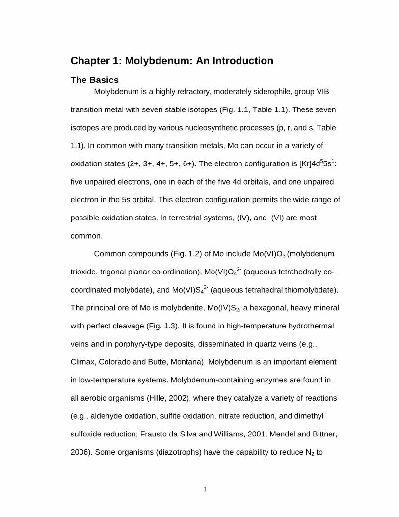
Common compounds (Fig. 1.2) of Mo include Mo(VI)O3 (molybdenum

trioxide, trigonal planar co-ordination), Mo(VI)O42- (aqueous tetrahedrally co-

coordinated molybdate), and Mo(VI)S42- (aqueous tetrahedral thiomolybdate).

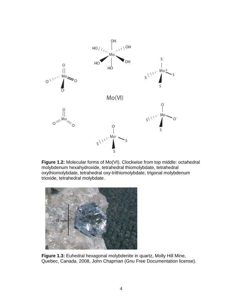
The principal ore of Mo is molybdenite, Mo(IV)S2, a hexagonal, heavy mineral

with perfect cleavage (Fig. 1.3). It is found in high-temperature hydrothermal

veins and in porphyry-type deposits, disseminated in quartz veins (e.g.,

Climax, Colorado and Butte, Montana). Molybdenum is an important element

in low-temperature systems. Molybdenum-containing enzymes are found in

all aerobic organisms (Hille, 2002), where they catalyze a variety of reactions

(e.g., aldehyde oxidation, sulfite oxidation, nitrate reduction, and dimethyl

sulfoxide reduction; Frausto da Silva and Williams, 2001; Mendel and Bittner,

2006). Some organisms (diazotrophs) have the capability to reduce N2 to

2

ammonia; one of the enzymes that is necessary for this process is an Fe-Mo

protein (dinitrogenase), which contains the site of N2 binding (Georgiadis et

al., 1992). Except for dinitrogenase (Rajagopalan and Johnson, 1992), all the

known molybdoenzymes contain a cofactor (molybdopterin), whose

biosynthetic pathway is universally conserved, implying that the pathway must

have appeared early in the history of life (Mendel and Schwarz, 1999).

3

Figure 1.1: Relative abundances of stable molybdenum isotopes.

Table 1.1: Terrestrial Mo isotope composition Mo Isotope Nuclidic massa Mole fractiona Processb

92 91.905810(4) 0.148362(148) p 94 93.9050867(20) 0.092466(92) p 95 94.9058406(20) 0.159201(159) s,r 96 95.9046780(20) 0.166756(167) s 97 96.9050201(20) 0.095551(96) s,r 98 97.9054069(20) 0.241329(241) s,r 100 99.907467(6) 0.096335(96) r

aCoplen et al., 2002. (IUPAC Technical Report, and references therein). b Wieser and De Laeter, 2007.

4

Figure 1.2: Molecular forms of Mo(VI). Clockwise from top middle: octahedral molybdenum hexahydroxide, tetrahedral thiomolybdate, tetrahedral oxythiomolybdate, tetrahedral oxy-trithiomolybdate, trigonal molybdenum trioxide, tetrahedral molybdate.

Figure 1.3: Euhedral hexagonal molybdenite in quartz, Molly Hill Mine, Quebec, Canada. 2008, John Chapman (Gnu Free Documentation license).

5

Molybdenum geochemistry in water and sediments The Mo concentration in ocean waters is relatively constant with

salinity (conservative, 10.5 µg/L; e.g., Bruland, 1983; Collier, 1985). This

concentration and the conservative nature of Mo are unusual for a biologically

essential trace element (Tribovillard et al., 2006). The residence time, (τ),

800,000 y, of Mo in seawater is also unusually long for a trace element

(Morford and Emerson, 1999). The long residence time of Mo suggests that

its highly soluble aqueous anion, molybdate, (Mo(VI)O42-) is relatively

unreactive in seawater. The main source of dissolved Mo to the oceans is

continental weathering products delivered through rivers, so the Mo

concentration of the input probably varies depending on the material being

weathered at any one time (e.g., Bertine and Turekian, 1973). For example,

where streams drain the area around the Climax molybdenite deposit

(Colorado), Mo concentrations in stream water are very high (10 mg/L;

Kaback and Runnells, 1980). In contrast, the Ottawa River, which flows

through granitic bedrock, has a very low Mo concentration (~0.2 µg/L; Archer

and Vance, 2008). Molybdenum concentrations in rivers draining regions with

black shales tend to be relatively high (2.3-10 µg/L; Colodner et al., 1993).

The paucity of processes that can remove Mo from seawater are

reflected in its generally long residence time in the ocean. In oxygenated

seawater, at marine pH, Mo is not adsorbed by many of the most common

constituents of oceanic sediments, such as clay particles, CaCO3, or Fe-

oxyhydroxides (Goldberg et al., 1998). The typical Mo concentration range of

these types of sediments is only 0.05-2 µg/g, similar to the concentrations in

6

average shale and average continental crust (Taylor and McLennan, 1985;

Rudnick and Gao, 2003). The major exceptions to limited removal are

hydrogenous Mn-oxyhydroxides, which form as nodules or crusts in oxic,

hemipelagic sediments, and have a high affinity for Mo (e.g., Calvert and

Price, 1977; Shimmield and Price, 1986). These types of sediments

accumulate at rates between a few mm per million years to hundreds of mm

per million years. Molybdenum concentrations in nodules range between 0.03

to 0.05 wt. % (Cronan, 1976). The nature of this sink, however, leads to an

important question regarding the mass balance of Mo in the oceans. Although

up to 90% of the ocean floor is oxic by some estimates, with manganese

deposits covering as much as 50% of some ocean basins (Glasby, 2000), the

flux of Mo to oxic sediments is estimated to be between only 20% (Morford

and Emerson, 1999) to 75% (Arnold et al., 2004) relative to river influx.

Consequently, the general steady-state with respect to Mo inputs and

removals likely requires an additional important sink. That sink is most likely

sediments formed under anoxic conditions. Indeed, anoxic sedimentary

regimes appear to sequester a quantity of the dissolved Mo influx that is

disproportionate to their extent in the oceans (only about 0.3% of the ocean

floor, Helly and Levin, 2004). Algeo (2004) calculated that in the Devonian,

the greater extent of anoxia in the oceans, coupled with a greater burial flux

accompanying formation of black shales could have drawn down the Mo

concentration of seawater and lowered its residence time to ~470,000 y.

Estimates for the removal of Mo to anoxic sediments range from 10-40% of

7

dissolved Mo in the oceans (Bertine and Turekian, 1973; Emerson and

Huested, 1991; Morford and Emerson, 1999). Any additional imbalance (10-

20%) might be accounted for by sedimentation in aqueous regimes that are

O2 depleted but not strictly anoxic (e.g., under oxygen minimum zones, such

as may be found under regions with strong coastal upwelling), so-called

'suboxic' sediments.

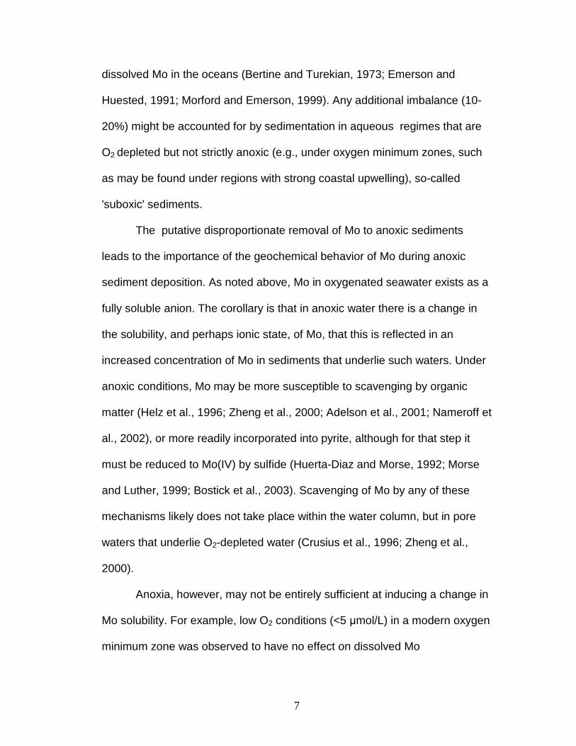
The putative disproportionate removal of Mo to anoxic sediments

leads to the importance of the geochemical behavior of Mo during anoxic

sediment deposition. As noted above, Mo in oxygenated seawater exists as a

fully soluble anion. The corollary is that in anoxic water there is a change in

the solubility, and perhaps ionic state, of Mo, that this is reflected in an

increased concentration of Mo in sediments that underlie such waters. Under

anoxic conditions, Mo may be more susceptible to scavenging by organic

matter (Helz et al., 1996; Zheng et al., 2000; Adelson et al., 2001; Nameroff et

al., 2002), or more readily incorporated into pyrite, although for that step it

must be reduced to Mo(IV) by sulfide (Huerta-Diaz and Morse, 1992; Morse

and Luther, 1999; Bostick et al., 2003). Scavenging of Mo by any of these

mechanisms likely does not take place within the water column, but in pore

waters that underlie O2-depleted water (Crusius et al., 1996; Zheng et al.,

2000).

Anoxia, however, may not be entirely sufficient at inducing a change in

Mo solubility. For example, low O2 conditions (<5 µmol/L) in a modern oxygen

minimum zone was observed to have no effect on dissolved Mo

8

concentrations (Nameroff et al., 2002). In order for Mo to become particle-

reactive, the presence of sulfide appears to be necessary, possibly as a direct

reactant in the formation of thiomolybdates, or Fe-Mo-S clusters that can be

easily scavenged (Helz et al., 1996; Erickson and Helz, 2000; Vorlicek et al.,

2004). Within the water column of the Black Sea, the concentration profile of

dissolved Mo with depth is approximately the opposite of the H2S profile (e.g.,

Emerson and Huested, 1991; etc), suggesting that removal is taking place

within the water column. However, in euxinic water columns, it has been

argued that there is no systematic relationship between sedimentary Mo and

H2S (e.g., Algeo and Lyons, 2006). In well-studied, seasonally anoxic, semi-

enclosed settings such as the Cariaco Basin, Saanich Inlet, and Framvaren

Fjord, profiles of the concentration of dissolved Mo show a tendency for Mo

concentration to decrease with depth (possibly at the interface between O2

and H2S), and the sediments that form to become enriched in Mo (Emerson

and Huested, 1991; Algeo and Lyons, 2006). This counter intuitively implies

that scavenging within the water-column does not take place, rather Mo

removal occurs at the sediment-water interface or in the sediments (Emerson

and Huested, 1991). Measurements of sulfide and Mo in pore waters suggest

that a sulfide threshold must be reached before Mo is removed (Colodner et.,

1993; Zheng et al., 2000), although behavior of Mo in pore water is

complicated by the cycling of MnOx at the redox boundary in the sediments

(Shimmield and Price, 1986; Calvert and Pedersen, 1993; Crusius et al.,

1996). The process of MnOx cycling has been shown re-deliver Mo to pore

9

waters below the redox boundary (e.g., Crusius et al., 1996; McManus et al.,

2002; Morford et al., 2005), at which point it can be fixed in a solid (sulfide)

phase (e.g., Calvert and Pedersen, 1993; Morford et al., 2009). Tribovillard et

al. (2004) emphasized the importance of sulfurized organic matter in trapping

Mo in the sediments. The concentration of aqueous H2S has been shown to

exert a control on the stepwise conversion of Mo(VI)O42- through a series of

thiomolybdate intermediates with the formula MoOxS4-x2-, beginning at a

geochemical switch point of 11 µM (Erickson and Helz, 2000). It is these

intermediates, and the final substituted thiomolybdate (Mo(VI)S42-), thought to

be the particle-reactive species, that are scavenged (Helz et al., 1996). Within

the sediments, these stepwise reactions probably proceed through 6-

coordinate, rather than 4-coordinate intermediates, and may be catalyzed by

clay mineral surfaces (Vorlicek and Helz, 2002). The thiomolybdates are likely

to be scavenged by pyrite (Bostick et al., 2003; Vorlicek et al., 2004), organic

carbon, and particularly, sulfurized organic matter (Tribovillard et al., 2004).

Furthermore, the trithio- and tetrathio-molybdate reactions may be kinetically

irreversible on short time scales, which has been shown by the survival of

MoS42- for long periods in oxygenated water (Erickson and Helz, 2000).

However, acidifying such a solution would serve to increase the rate of

conversion from MoS42- to MoO4

2- (Erickson and Helz, 2000).

The relationship between Mo content and organic carbon (Corg or TOC)

is also somewhat contentious. Because of the positive correlation between

the two parameters in anoxic settings (Brumsack, 1986; Nijenhuis et al.,

10

1999; Warning and Brumsack, 2000; Werne et al., 2002; Algeo, 2004), Mo

concentration has been used as a redox proxy. However, Tribovillard et al.

(2004) showed high degrees of correlation only between Mo/Al and one

particular subtype of organic matter, specifically sulfurized (orange) organic

matter. In contrast, Wilde et al. (2004) argued that Mo/Al could be used as a

proxy for original TOC content, based on the high degree of correlation.

Lyons et al. (2003) found only a weak correlation between Corg and Mo/Al in

Cariaco Basin sediments that were deposited under euxinic conditions. Algeo

and Lyons (2006) proposed that the uptake of Mo at the sediment-water

interface is dominated by organic 'host phases', and that this explains the Mo-

TOC covariation in anoxic environments. However, there are limits to Mo and

TOC enrichment, which include the Mo drawdown, deepwater renewal time,

and amount of stagnation (Algeo and Lyons, 2006). As an example, if an

anoxic setting did not receive a periodic renewal of oxygen and dissolved Mo,

its degree of stagnation would increase, and the drawdown of Mo to the

sediments would eventually lead to a long-term trend towards lower Mo/TOC

ratios. Thus, Mo/TOC has been proposed to be a better proxy for degree of

water mass restriction, as opposed to Mo alone being a straightforward proxy

for redox state in the water column (Algeo and Lyons, 2006; Algeo et al.,

2007; Scott et al., 2008).

Covariation of Mo with pyrite has also been a subject of debate. On

one hand, there is some evidence that Mo is positively correlated with the

pyrite content of host sediment (Huerta-Diaz and Morse, 1992; Crusius et al.,

11

1996; Tribovillard et al., 2008). Further, a modicum of data suggest that Mo

readily enters Fe-S phases (Bostick et al., 2003), and a second study

suggests that pyrite framboids may sequester Mo from overlying oxic water,

during formation in shallow 'suboxic' sediments (Tribovillard et al., 2008).

Other studies, however, have presented opposing evidence, e.g., for a lack of

correlation between pyrite and Mo (Lyons et al., 2003). A key point with

respect to correlations between Mo and pyrite may be the Corg concentration

of the sediments, as this parameter appears to control the capacity for H2S

generation (Lyons et al., 2003). Microbially-mediated degradation of

accumulated organic matter generates sulfide (from sulfate reduction), which

reacts with Fe2+ to form pyrite (e.g., Passier et al., 1996). This has led to

proposals that pyrite formation may be controlled by the availability of reactive

Fe phases (FeOx), rather than organic carbon (Raiswell and Canfield, 1998).

As mentioned above, sulfurized organic matter strongly correlates with Mo

content. However, sulfurized organic matter can only form when H2S begins

to accumulate, because H2S formation has outstripped the supply of reactive

Fe (Tribovillard et al., 2004). This, in turn, can only occur after FeOx has been

consumed (Raiswell and Canfield, 1998). Thus, pyrite formation appears to

occur before organic matter is sulfurized (Tribovillard et al., 2004, and

references therein).

Summary

The geochemistry of Mo in sediments appears to be controlled by the

dichotomous behavior in aqueous environments: soluble under oxic

12

conditions, but becoming increasingly labile as the water column looses

oxygen. Thus, Mo has potential for use as a proxy for organic carbon, for

water column anoxia, and in conjunction with other parameters, for degree of

water-mass restriction. However, full realization of the potential strengths of

Mo as a proxy has been somewhat constrained by incomplete understanding

of the mechanisms by which Mo is sequestered into sediments, the exact

form in which it exists in the sediments, and in what sedimentary component it

resides (e.g., pyrite versus sulfurized organic matter). These and similar

topics continue to foster discussion and new research. In recent years, the

use of Mo isotopes has been added to the tools for addressing these topics.

Molybdenum isotopes Measurement of Mo isotopes in meteorites is fairly common (Murthy

1962, 1963; Wetherill, 1964; Qi-Lu and Masuda, 1992; Lee and Halliday,

2003; Nicolussi et al., 1998; Yin and Jacobsen, 1998; Dauphas et al., 2004).

However, the goal of these studies was to identify mass-independent

(nucleosynthetic) isotopic anomalies, as well as evidence for Tc decay in

97Mo. The internal normalization used to correct for instrumental fractionation

in such studies precludes measurement of natural, mass-dependent

differences. Additionally, Mo isotopes have also been used to study Mo

metabolism in the body (e.g., Turnlund et al., 1993; Turnlund et al., 1995;

Sievers et al., 2001; Keyes and Turnlund, 2002). The first of these (Turnlund

et al., 1993) utilized chromatographic separation (nearly identical to that

13

currently in use by geologists), combined with a triple-spike method and

analysis by TIMS.

The geochemistry of Mo, and specifically its sensitivity to

environmental reducing conditions, result in its utility as a proxy for the

general redox state of a water column. In the search to refine redox

interpretations of ancient sediments, Anbar et al. (2001), performed

experiments of chromatographic separation of Mo and MC-ICP-MS (Multi-

collector inductively -coupled plasma mass spectrometry) measurement of

Mo isotopes using external fractionation correction. This was done in the

hope that mass dependent variations might: 1) be found, and 2) be related to

environmental conditions during deposition. A short time later, a different

research group published a double-spike method for internal fractionation

corrected Mo isotope analysis by MC-ICP-MS (Siebert et al., 2001). Both

groups tested their respective methods on molybdenites (MoS2; porphyry

versus hydrothermal), and obtained positive results, in the sense that isotopic

fractionation was observed (±0.3‰ in δ98Mo1). The two methods, however,

differed in the external standard reproducibility associated with the

measurements. The external fractionation correction method had a published

2σ of ±0.2‰ for standards, while the double-spike method was able to

produce standard data with 2σ ±0.06‰, a significant improvement. 1Generally, in the remainder of this work, all Mo isotopic compositions will be reported as δ98Mo. This is done to introduce consistency in the nomenclature, as some working groups use different isotopes in the ratio. Conversion between 97Mo/95Mo and 98Mo/95Mo is achieved by dividing by 2/3, thus, no attempt will be made to identify where the original published data were reported using a different notation.

14

As an important side note, comparison of Mo isotope data from

different labs suffers from the lack of a true recognized isotopic standard. The

majority of researchers use SpecPure® Mo, or a similar material, as a

normalizing standard, and define the isotopic composition of this material to

be 0‰. It is not known how individual batches of this Mo solution might vary

isotopically. Thus, data normalized using one batch would be internally

consistent, but might not be consistent with data normalized using a different

batch.

Once it was established that mass-dependent variations exist in a

geological materials, and could be adequately resolved for some purposes,

the next step was to determine the isotopic composition of Mo reservoirs and

sinks (Fig. 1.4). In order to be able to make any interpretive statement about

ancient sediments, the modern system needed to be quantified. Barling et al.

(2001) showed that there was a large fractionation between the seawater

molybdate reservoir (δ98Mo=+2.3‰) and Mn oxyhydroxide (MnOx) nodules

(δ98Mo average -0.8‰), which were noted in the preceding section to be a

quantitatively important Mo sink on long time scales. The isotopically heavy

nature of seawater was demonstrated to extend to three major oceans, and

be constant with depth (Siebert et al., 2003). Siebert et al. (2003) confirmed

removal of isotopically light Mo to MnOx in two nodules, and the constant

offset from seawater over a 60 Ma 'transect' in the nodules was taken as

evidence that the δ98Mo of seawater had not changed significantly in that time

period. Samples of basalt, granite, and clastic sediment were measured and

15

found to have δ98Mo values ranging from 0‰ to 0.3‰, suggesting that the net

effect of transport and weathering processes does not affect δ98Mo (Siebert et

al., 2003).

Euxinic Black Sea sediments were shown to have δ98Mo from +1.6 to

+2.4, from which it was inferred that a highly efficient removal process from

overlying sulfidic water acted on this system (Barling et al., 2001). Anoxic

sediments were shown to display a fairly constant offset from seawater by

-0.7‰ (McManus et al., 2002; Poulson et al., 2006). These observations have

been frequently applied to the idea that the extent of anoxic/euxinic

sedimentation in the past can be calculated if the isotopic compositions of the

Mo input and oxic Mo sink are known (Arnold et al., 2004; Siebert et al., 2005;

Wille et al., 2007; Pearce et al., 2008; Wille et al., 2008; Lehmann et al.,

2007). Estimates of anoxic sedimentation made in this way have been used

to assess the oxygenation state of the ancient ocean/atmosphere. However,

as the Mo isotope data set has broadened, this type of calculation has been

shown to be too simplistic to well describe natural systems. There are several

important complications inherent to this type of modeling. The first is that

'suboxic' authigenic Mo formation constitutes an important sink for Mo (10-

20%), and the δ98Mo values that have been measured in 'suboxic' sediments

span a large range (-0.5 to +1.3‰), with no constant offset from seawater

(Siebert et al., 2006; Poulson-Brucker et al., 2009).

Secondly, recent measurements of δ98Mo in rivers (Archer and Vance,

2008) have shown that rivers are isotopically disparate (+0.2 to +2.4‰), and

16

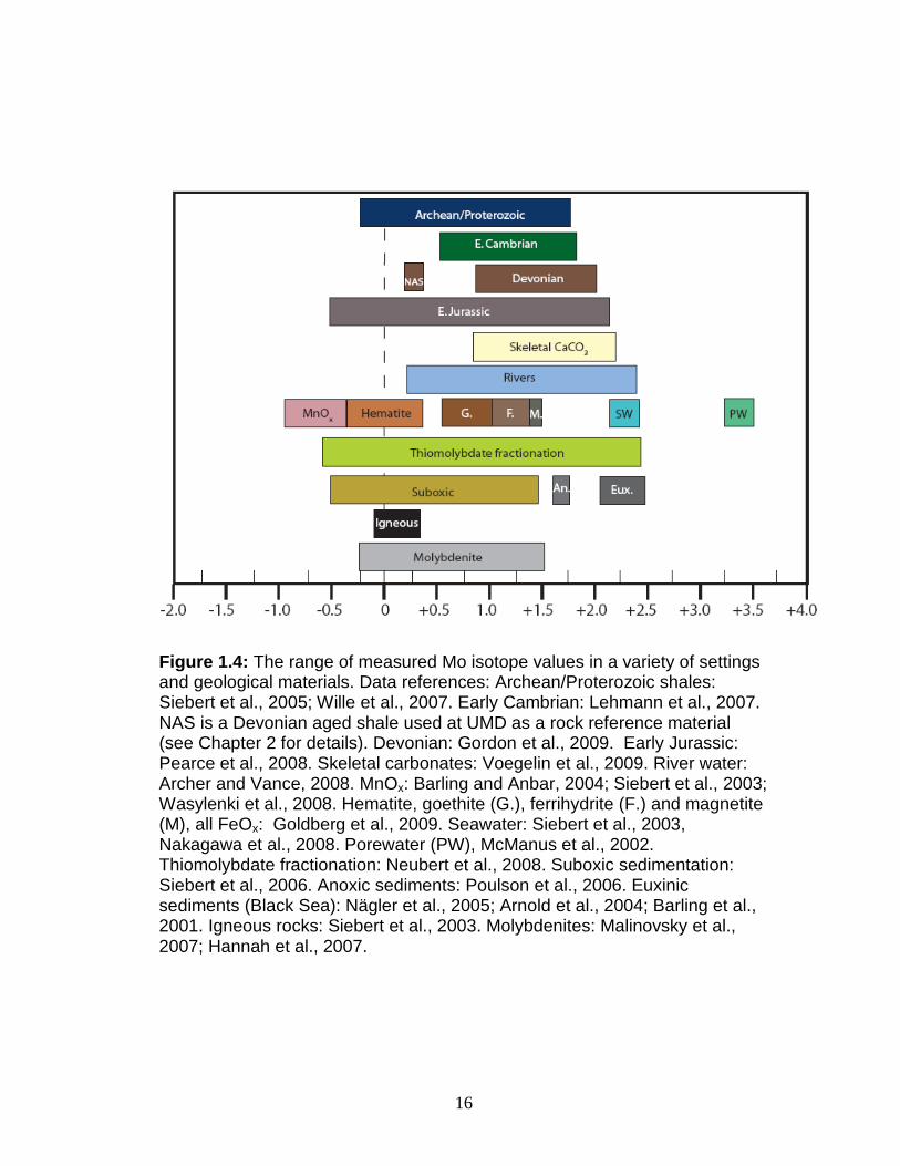
Figure 1.4: The range of measured Mo isotope values in a variety of settings and geological materials. Data references: Archean/Proterozoic shales: Siebert et al., 2005; Wille et al., 2007. Early Cambrian: Lehmann et al., 2007. NAS is a Devonian aged shale used at UMD as a rock reference material (see Chapter 2 for details). Devonian: Gordon et al., 2009. Early Jurassic: Pearce et al., 2008. Skeletal carbonates: Voegelin et al., 2009. River water: Archer and Vance, 2008. MnOx: Barling and Anbar, 2004; Siebert et al., 2003; Wasylenki et al., 2008. Hematite, goethite (G.), ferrihydrite (F.) and magnetite (M), all FeOx: Goldberg et al., 2009. Seawater: Siebert et al., 2003, Nakagawa et al., 2008. Porewater (PW), McManus et al., 2002. Thiomolybdate fractionation: Neubert et al., 2008. Suboxic sedimentation: Siebert et al., 2006. Anoxic sediments: Poulson et al., 2006. Euxinic sediments (Black Sea): Nägler et al., 2005; Arnold et al., 2004; Barling et al., 2001. Igneous rocks: Siebert et al., 2003. Molybdenites: Malinovsky et al., 2007; Hannah et al., 2007.

17

in the case of the Nile, there are seasonal differences in δ98Mo (+0.2 to

+0.8‰). In this work (Chapter 3), the δ98Mo of the Susquehanna River was

measured and found to fall within this range (1.1‰). The apparent range of

positive δ98Mo values for river input has several implications: 1) it cannot be

assumed that transport and erosion have no effect on the δ98Mo of materials

being weathered, and 2) it cannot be assumed that weathered materials start

with a δ98Mo near zero. Indeed, evidence from molybdenite deposits indicates

that a large range in δ98Mo can be generated via relatively high-temperature

processes (-0.3 to +1.5‰, Hannah et al., 2007; Malinovsky et al., 2007).

Furthermore, the δ98Mo of molybdenite was shown to effect the δ98Mo values

of sediments in lakes close to the molybdenite occurrence (Malinovsky et al.,

2007). While molybdenites are unlikely to be a major source of Mo to the

oceans, several studies have demonstrated that continental materials formed

by high temperature igneous or metamorphic processes can have significant,

non-zero δ98Mo values (Wieser and DeLaeter, 2003; Pietruszka et al., 2006;

Hannah et al., 2007; Malinovsky et al., 2007). A comprehensive survey of

δ98Mo in igneous rocks is needed to determine if the isotopic range observed

in rivers is the result of source or alteration/weathering processes.

Yet a third complication to the simple idea that the δ98Mo value of a

euxinic sediment reflects the δ98Mo value of seawater is evidence from the

Black Sea itself, which is arguably the best modern example of sedimentation

under a euxinic water column. In the Black Sea, the H2Saq concentration is

18

near zero at the surface, begins to rise at the chemocline (~100 m depth), and

is high and fairly constant below ~400 m depth (Neretin et al., 2001). This

systematic variation was used to calculate the speciation of molybdate to

thiomolybdate with depth (i.e., increasing H2Saq), from which came the

concept of the geochemical 'switch point' at 11µM H2Saq, where water column

scavenging of Mo becomes dominant (Erickson and Helz, 2000). In a study of

δ98Mo values in Black Sea sediments deposited under different H2Saq

conditions, a wide range of values (-0.1 to +2.5‰) was found (Neubert et al.,

2008). Combining the calculated δ values between individual Mo species

(Tossell, 2005) with the model of Erickson and Helz (2000), Neubert et al.

were able to provide support for the calculations of Tossell (2005), who

predicted that large fractionations might result from a 'partial' removal by

equilibrium fractionation.

The fractionation of Mo isotopes during adsorption to Mn-oxides has

now been shown to be insensitive to pH changes (Barling and Anbar, 2004),

ionic strength, and is not greatly affected by temperature (0.3‰ difference

over 50°C; Wasylenki et al., 2008). The formation of MnOx and adsorption of

light Mo has been proposed to be the cause of isotopically heavy pore water

(McManus et al., 2002). However, MnOx are readily dissolved when buried to

the redox boundary in sediments. The release of isotopically light Mo to the

pore water (McManus et al., 2002), and subsequent uptake in authigenic

sediments is thought to overprint the δ98Mo values of any existing authigenic

minerals (Reitz et al., 2007; Chapter 4, this work). Recently, evidence of Mo

19

fractionation during adsorption to Fe-oxy(hydroxides) has been reported, and

the range of δ98Mo values of Mo adsorbed to these minerals overlaps with the

suboxic range (Goldberg et al., 2009). Since FeOx forms are important

components of aqueous sediments (Poulton and Raiswell, 2002), and can

adsorb Mo (Goldberg et al., 1998), they may provide an additional important

sink for Mo.

Finally, uptake of Mo has been shown to produce a range of δ98Mo

values in carbonates, although the amount of Mo that is sequestered in most

carbonates is very small, <0.1µg/g (Voegelin et al., 2009). Skeletal carbonate

phases, which dominate some marine sediments, have generally heavy

δ98Mo values, from gastropods of +0.7‰ to coral of +2.2‰ (Voegelin et al.,

2009). These authors proposed that there is no effect of local redox

conditions on Mo uptake to carbonates, but there is a biological effect in

skeletal samples. Thus, non-skeletal ooids might be useful as a proxy for the

δ98Mo of the ambient seawater (Voegelin et al., 2009).

Additionally, it has been proposed, but not empirically proven, that Mo

isotopes may be fractionated during adsorption to sinking or in-situ organic

matter (Poulson-Brucker et al., 2009). Small fractionations (-0.5‰) have been

shown to occur during uptake to the soil bacterium Azotobacter vinelandii

(Wasylenki et al., 2007; Liermann et al., 2005), which requires Mo for N2

fixation, and there is reason to believe that similar fractionations may be

evidenced by aqueous N2-fixing organisms, which share a biosynthetic

pathway for the enzyme nitrogenase. Thus, if aqueous cyanobacteria were

20

abundant, under the appropriate conditions, microbial fractionation of Mo from

the water column might be observable. This would probably require an anoxic

water column, so that active nitrogen fixation could occur. If the flux of

cyanobacterial biomass and fractionated Mo was large enough, it might be

possible to see evidence for it in a sediment sample.

The contributions of this work Several projects have been completed that will contribute to the

understanding of Mo and Mo isotopes in geochemical systems. The first of

these projects was to assess the behavior of Mo in the sediments and waters

of Chesapeake Bay and its main tributary, the Susquehanna River (Chapter

3). The original idea behind this study was to determine whether Mo isotopes

could track the onset, and document the severity of, coastal eutrophication

and anoxia in the Bay. The Mo isotope data did not show a strong signal of

anoxic deposition, but there was a trend towards increasing variability of

δ98Mo values, that was interpreted to indicate an increase in the incidence of

coastal anoxia. It was also demonstrated that Mo isotopic fractionation was

occurring within the Susquehanna river basin, and that Mo removal from the

water column is taking place within the Chesapeake Bay. This work has been

accepted for publication by Earth and Planetary Science Letters, and is co-

authored by George Helz and Rich Walker.

The second large project was to investigate Mo isotope signatures in

Pliocene-Pleistocene-aged core samples from the Mediterranean Sea

(Chapter 4). The Mediterranean sediments include numerous organic-rich

21

layers that are called sapropels. These unusual sediments are thought to

form when fresh water influx to the sea surface prevents convective mixing,

leading to an episode of anoxia in the deep water, possibly combined with an

increase in surface productivity. The project ultimately included not only Mo

isotopes and Mo concentrations, but Re concentrations, major elements, and

a small number of sulfur isotopic analyses. The main result of the study is that

the conditions under which sapropels can form seem to vary significantly from

episode to episode. These variations are apparent in all of the proxies that

were examined, including Mo isotopes. This work is currently being prepared

for submission.

The publication of molybdenite δ98Mo data with a large and non-

systematic range of values provided the impetus for a collaboration with

Michael Mengason of the Laboratory for Mineral Deposits Research (UMD).

Michael performed a number of experiments that were designed to determine

whether fractionation of Mo takes place between a vapor phase and a melt

phase at high temperature and pressure. The resultant run products were

processed and analyzed for Mo isotopes. There appears to be a fairly

systematic fractionation between the two phases, with the vapor phase being

isotopically heavier. These results are presented in Chapter 5. We intend to

publish a short paper that describes these data. Michael contributed the

experimental products and knowledge of porphyry Mo deposits, while I

contributed the Mo concentration and isotope measurements and background

information in these topics.

22

Chapter 2: Method development at UMD

First attempts The development of high sensitivity, high resolution multi-collector

inductively coupled plasma mass spectrometry in 1992 (MC-ICP-MS)

instigated a tide of research into the isotopic compositions, fractionation

mechanisms, and behavior of the heavy transition elements (e.g., Cr, Fe, Cu,

Zn, Mo), and other, 'non-traditional' stable isotopes (e.g., Li, Mg, Ca; see

Johnson, Beard and Albarede, Eds., 2004, for a review). The first attempts at

analyzing mass-dependent Mo isotope variations by MC-ICP-MS came in

2001 (Anbar et al,. 2001 and Siebert et al., 2001), and proved feasibility for

future developments in the methodology, as discussed in Chapter 1. On a

historical note, Murthy (1962, 1963) and Wetherill (1964) both attempted to

measure Mo isotope variations in meteorites (stony and iron), but were

hampered by analytical uncertainties, despite Wetherill's use of a double

spike. This usage was one of the first practical applications of a double spike

method. The primary difficulty of assessing the natural fractionation of Mo

isotopes lies in precisely compensating for mass bias imparted during

processing and analysis, because the total measured range of variation in

δ98Mo in earth materials is typically less than 4‰ (Anbar et al., 2001).

The groundwork for Mo isotope measurements at UMD was laid by

Aaron Pietruszka, circa 2003-2004, who developed the preliminary

chromatographic methods, and performed several series of Mo isotope

measurements on solution standards, and sample material with simple

matrices (molybdenites) using the UMD Nu-Plasma MC-ICP-MS (Pietruszka

23

et al., 2006). This work was the first to identify a large range in molybdenite

Mo isotopic composition (-0.75 to +1.05‰). These measurements also

determined that matrix effects for solution standards could be controlled with

careful analytical techniques (Pietruszka et al., 2006). The path from these

initial successful measurements to the high-precision measurement of more

complex matrices has been lengthy. A discussion of the steps taken is

presented here, as well as a summary of the methods currently in use.

Brief overview of MC-ICP-MS The Nu-Plasma MC-ICP-MS instrument is double-focusing

(electrostatic analyzer and a magnetic sector analyzer, in Nier-Johnson

geometry), equipped with variable zoom optics for beam focusing, and 12

faraday detectors (Belshaw et al., 1998). In the simplest terms, mass

spectrometry relies on the behavior of ions accelerated through a potential

into a magnetic field, where the deflection of the ion's flight path through the

field is determined by its mass to charge ratio (M/Z). The accelerated,

deflected ions impact detectors, which record the number of ions per unit time

as current. The current passes through a resistor with known specific

resistivity (1011 Ω), which generates a voltage that is measured (V = I * R).

Mass spectrometers differ in two fundamental aspects: how ions are created

at the sample-input end, and the way in which the mass and number of ions is

determined. The former must take into account the first ionization potential of

the element; for elements with low to intermediate ionization potentials, gas-

source or thermal ionization (TIMS) can be used, but elements with high

24

ionization potentials require a higher energy method such as a plasma.

Although Mo can be ionized by thermal processes, its high first ionization

potential of 684 kJ/mol means it is well suited for ionization by ICP. At the

ionization temperature, 98% of Mo is ionized (Houk, 1986). The latter aspect

takes into account whether the user wishes to measure element or isotope

abundances, or element or isotope ratios. For precise isotope ratios, an

instrument with multiple detectors is best, while for element abundances, a

single-detector is better. This relates to issues with magnet hysteresis when

analyzing over a large mass range. Here the discussion will focus on MC-

ICP-MS, as the majority of the present work has focused on high precision

and accurate isotope ratios.

In instruments that utilize ICP as the ion source, argon gas is generally

used as the carrier gas as well as the 'source' gas. A cylindrical (induction)

coil is wound around a quartz torch; a time-varying electrical current, supplied

by a radio-frequency generator (at 27 MHz), is passed through the coil, which

induces variable magnetic fields in the gas. A spark plug supplies the first

electrons to interact in the magnetic field. Argon atoms are ionized and create

a plasma with temperatures between 6000 and 10000 K. Samples are

introduced as aerosols, and are indiscriminately ionized in the plasma. The

ions created have a range of kinetic energies, which necessitates the use of

an electrostatic filter (Albarede and Beard, 2004).

The Plasma Laboratory possesses several devices for sample

introduction. The two nebulizers used for Mo work (ESI Apex and CETAC

25

Aridus) both operate on the same principle of desolvation. A liquid sample is

introduced to the apparatus at a flow rate of ~40 µl/min, which is assessed

before each analytical session. The liquid sample, passes through a heated

membrane or chamber, where the solvent evaporates. The remaining solute

is passed into the torch in a stream of sampling gas.

Mass bias and instrumental fractionation Mass bias, or instrumental mass fractionation, refers to the variable

transmission of the ion beam into the mass spectrometer. It is a significant

drawback of ICP-MS, where there is a strong preferential transmission of

heavier ions (Wombacher and Rehkämper, 2003). The majority of mass bias

occurs in the source or source-mass analyzer interface, as opposed to within

the mass analyzer, flight tube, or collectors (Albarede and Beard, 2004). For

example, changes in the geometry of the skimmer cone can have a large

effect on the mass bias; distance of the torch from the sample cone; or matrix

effects. In ICP-MS, the degree of mass fractionation is significantly larger

compared to TIMS, but is nearly time-invariant (Wombacher and Rehkämper,

2003). These effects can have major implications for stable Mo isotope

measurements.

Three types of laws are commonly used to describe and correct for

mass bias (linear, exponential, and power laws). Fractionation in ICP-MS can

best be described with the exponential law. Here, the exponential law is

given, using two Mo isotopes (98Mo and 95Mo) as an example.

26

(2.1) 98/95true = 98/95measured * (98mass / 95mass)β

1.52445 = 98/95measured *(97.905408/94.905842)β

β=(log(1.52445/98/95measured))/(log(97.905408/94.905842))

In MC-ICP-MS, the fractionation factors (β) are generally less than -2, and

remain fairly constant for a given element (at UMD, βMo = -1.718 ± 0.009). A

correction in the measured ratio of a sample based solely on the exponential

mass bias law is called 'internal normalization'.

Matrix effects can also be a source of significant mass bias and must

be carefully eliminated. The term 'matrix effect' encompasses two main types

of phenomena. The first is the range of isobaric or spectral effects: direct

(e.g., 96Zr at 96Mo); oxides or nitrides (e.g., 84Kr16O at 100Mo); and doubly

charged species (e.g., 190Os2+ at 95Mo). The non-spectral effects are due to

the presence of other elements in the purified sample, which can cause

changes in the sensitivity of the element of interest. This change in sensitivity

can alter the mass bias, and significantly affect the accuracy of

measurements (Albarede and Beard, 2004). To illustrate this, the effect of a

variety of elements (Mn, Fe, Al, V, Zn) on the accuracy of Mo isotope

measurements was tested, by adding these elements to a standard reference

material (Fig. 2.1). The standard used was a gravimetrically prepared solution

made from a Mo wire. For this experiment, the wire standard was

27

Figure 2.1: The matrix effect on δ9x/95Mo of the UMD wire standard (black), using V (red), Al (blue), Fe (green), Mn and Zn (grey), Zn (purple), and Mn (orange). All samples had Zr added for external normalization. For Zn and Mn, the error bars are the standard deviation of the number of measurements (3 and 7, respectively). A single measurement was made for the other elements. The 2σ error of a typical δ9x/95Mo value is shown for reference. Β refers to ratios corrected with the fractionation factor β obtained using Zr. 97(2) uses the ratio taken during cycle 2 of the analysis.

28

Diluted to 800ng/g Mo, 200 ng/g Zr was added and the elements were added

to separate aliquots. The elements were added in the following quantities: V,

0.01ng; Al, 0.01ng; Fe, 0.078ng; Zn, 12 ng; Mn, 0.078 ng and 200 ng; Mn +

Zn, 12 ng + 0.078 ng. These experiments illustrate the negative effect of

impurities in a sample on the accuracy of measured Mo isotope ratios. In

many cases, the δ9x/95Mo value of the impure samples lies well outside the

accepted standard deviation of these measurements. One problem is that

these types of effects are not reproducible from sample to sample, as

illustrated by the large range of values from repeated measurements of the

standard plus Zn or Mn.

Both general types of matrix effect can be controlled to a large extent

by ensuring that the separation/purification chemistry is effective at removing

everything but the element of interest. The cleanliness of the chemistry can

be checked for each sample measurement by scanning through the periodic

table. For Mo measurements, scans from mass 50 (Cr) through mass 91 (Zr)

and from mass 101 (Ru) to mass 120 (Sn) were checked for interfering

elements.

Pietruszka and Reznick (2008) showed that a standard passed through

an anion column was isotopically lighter than the same standard measured

directly, likely as the result of an organic residue sourced in the anion resin

itself, causing a matrix effect in the plasma. This 'column matrix effect'

generated an isotope effect that encompassed ~25% of the natural variation

in δ97/95Mo (Pietruszka and Reznick, 2008).

29

Methods for fractionation correction The primary difficulty of assessing the natural fractionation of trace

metal stable isotopes is compensating for mass bias during analysis. The

natural equilibrium fractionation of elements tends to decrease with increasing

temperature and increasing mass, as the relative mass difference between

isotopes of an element becomes small (Urey, 1947). For example, the known

range of variation in δ98Mo in natural samples is only ~5‰, compared to

~60‰ for δ7Li. Thus, correcting for the effects of analytical mass fractionation

must be increasingly precise with higher-mass elements. Three commonly

used techniques for fractionation correction will be discussed here, all of

which were, or are, used at UMD for Mo isotope analysis.

Sample-standard bracketing

The first, and probably simplest, method for assessing and correcting

for mass bias is termed sample-standard bracketing (SSB). The technique

works on the assumption that mass bias is constant between samples and

standards. In ICP-MS, the mass bias is large but is not subject to drift, so

SSB can be used successfully. A standard with known mass bias is run

before and after a sample with unknown mass bias, and the knowns are used

to interpolate the mass bias in the sample (Albarede and Beard, 2004).

External fractionation correction

Instrumental mass bias is often corrected by external fractionation

correction (FC). This refers to the addition, before analysis, of some amount

of a different element with isotopic masses within the range of the element of

interest (e.g., Belshaw et al., 1998). The principle behind external FC is that

30

the amount of mass bias for the element of interest can be calculated from

mass difference measured in the added element (e.g., Walder et al.,1993;

Marechal et al., 1999). However, the ability to measure accurate ratios for the

isobaric isotopes may be compromised, and the fractionation of the two

elements may not be identical. This method is applicable as long as the

sample has been completely purified of the element that will be added,

because its presence in the sample might alter the fractionation correction

factor.

External FC can be combined with SSB to provide, in theory, an even

better control on instrumental mass fractionation. However, 'automatrix'

effects can result in two ways: by allowing the ratio of the sample element and

added element to vary significantly between the bracketing standard and

sample; and by allowing the concentration of the sample element to vary

between standard and sample (Pietruszka et al., 2006).

Both SSB and external FC correct solely for instrumental mass bias,

and cannot provide any correction for mass fractionation during sample

processing. For example, it has been shown that ion exchange

chromatography can isotopically fractionate heavy elements such as Fe and

Cu, but that fractionation can be reduced if the elemental yield off the column

is close to 100% (e.g., Anbar et al., 2001; Marechal et al., 1999).

Double-spiking

Double-spiking is another technique for precisely determining the true

isotopic composition of an element in a sample, provided the element has

31

four or more isotopes. The technique involves the addition of two 'spike'

isotopes with known concentrations and isotopic compositions, and provides

a completely internal mass fractionation correction (Pietruszka et al., 2006).

Double-spiking was first outlined mathematically by Dodson (1963) and has

since been applied to many elements (Pb, Compston and Oversby, 1969;

Galer 1999; Ca, Russell et al., 1978; Nägler et al., 2000; Ba, Eugster et al.,

1969; Sr, Hofmann, 1971; Fe, Johnson and Beard, 1999, Dideriksen et al.,

2006; Se, Johnson et al., 1999, Herbel et al., 2000; Cr, Schoenberg et al.,

2008; Mo, Wetherill 1969, Siebert et al., 2001; S, Mann et al., 2008; Zn,

Bermin et al., 2006; Ge, Siebert et al., 2006; U, Stirling et al., 2007; Cd,

Ripperger and Rehkämper, 2007; Os, Markey et al., 2003).

The method can yield extremely precise fractionation-corrected values,

but is subject to some of the same limitations as other measurement

techniques; for example, clean sample separation and low blank are equally

important in double-spiking, although quantitative yields are less so. Double-

spiking may be more susceptible to memory effects in ICP-MS (Albarede et

al., 2004). Finally, in order for double-spiking to be successful, the spike and

sample must be equilibrated before any processing takes place, so that

fractionation occurring after the equilibration step will affect the sample and

spike to an equal degree (e.g., Johnson and Beard, 1999).

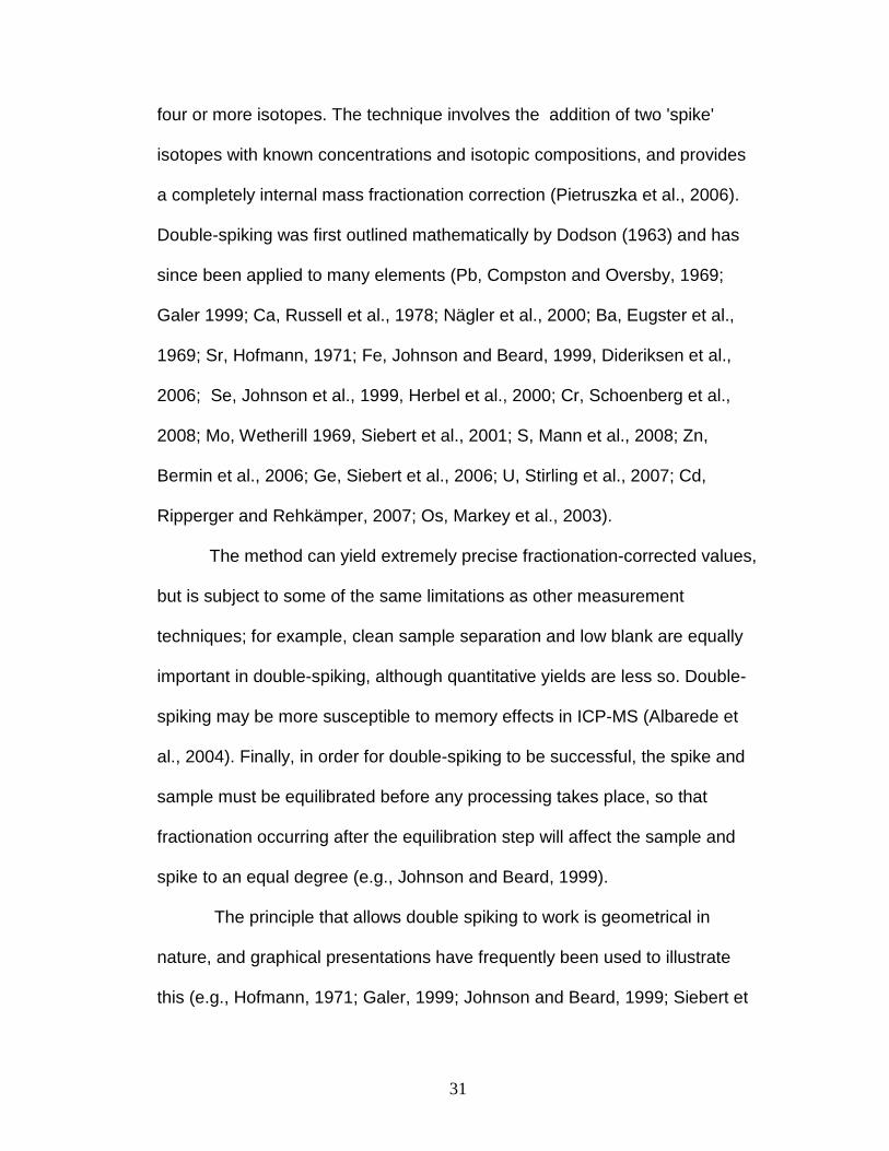
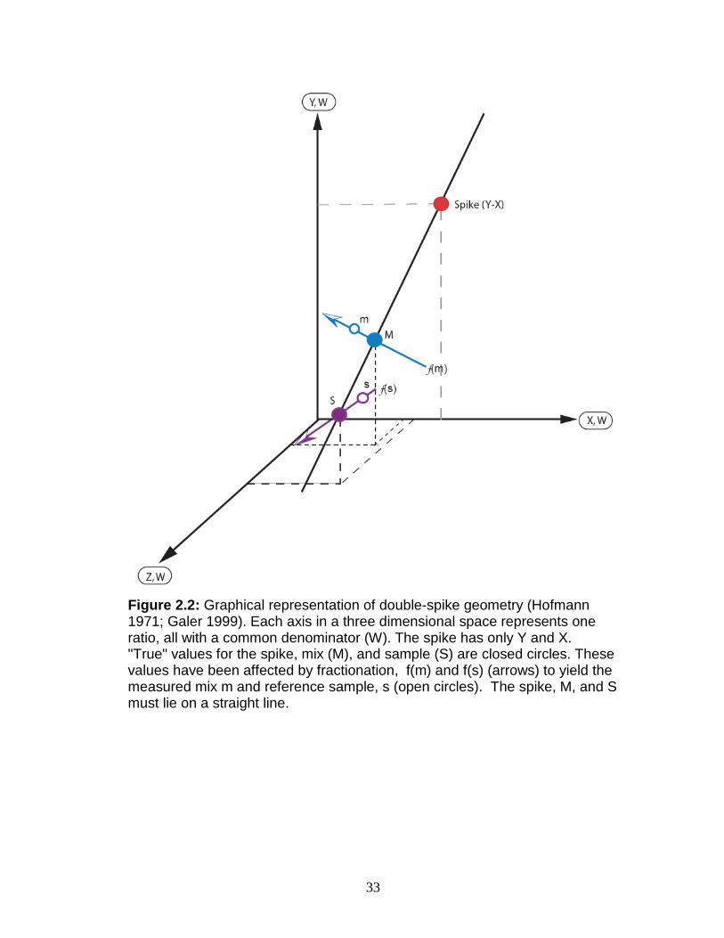
The principle that allows double spiking to work is geometrical in

nature, and graphical presentations have frequently been used to illustrate

this (e.g., Hofmann, 1971; Galer, 1999; Johnson and Beard, 1999; Siebert et

32

al., 2001; Albarede and Beard, 2004). For figures 2.2 and 2.3, each axis

represents a ratio of two isotopes with all ratios having a common

denominator. Only one possible mixing tie-line exists that connects the spike,

the true mix (M), and the true sample (S) compositions (Hofmann, 1971;

Galer, 1999; Johnson and Beard, 1999). The composition of M has been

affected by instrumental mass fractionation, f(m), to generate m, the

measured mix. The composition of S is approximated by using a reference

value (s) that has been affected by 'natural' fractionation, f(s). This is a valid

approximation because, with heavier elements, the range of fractionation is

relatively small (Albarede and Beard, 2004). The spike, m, and s do not share

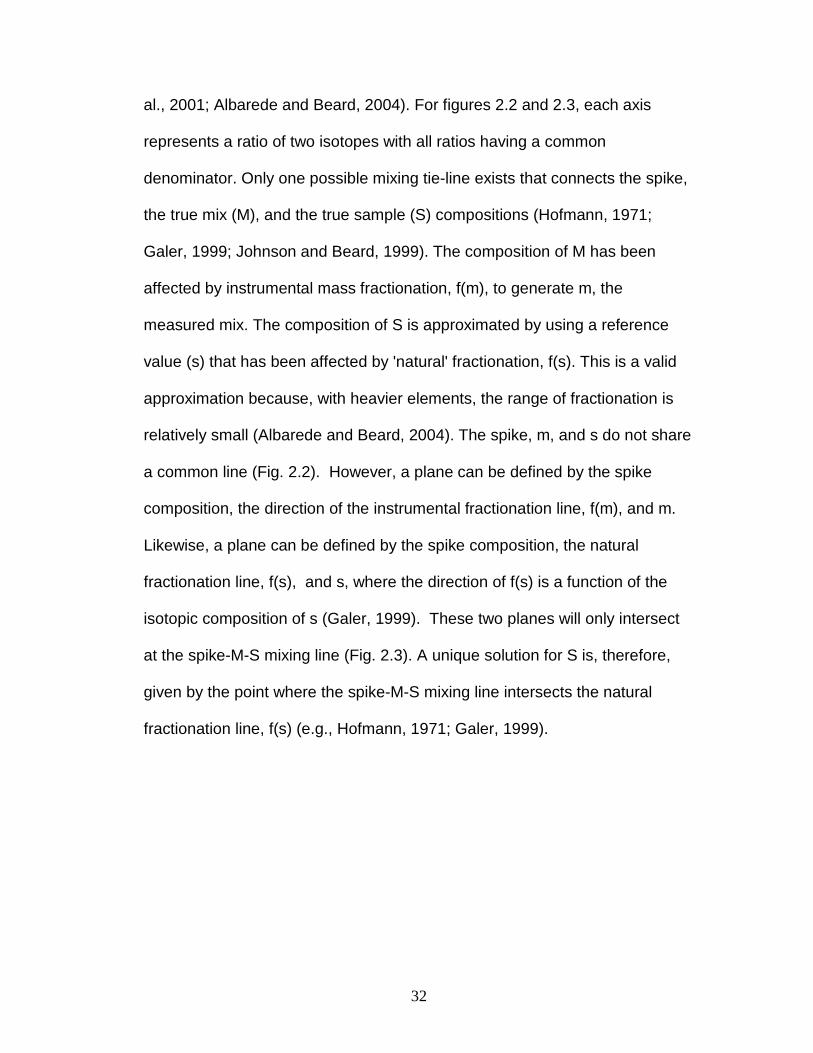
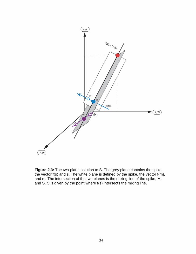
a common line (Fig. 2.2). However, a plane can be defined by the spike

composition, the direction of the instrumental fractionation line, f(m), and m.

Likewise, a plane can be defined by the spike composition, the natural

fractionation line, f(s), and s, where the direction of f(s) is a function of the

isotopic composition of s (Galer, 1999). These two planes will only intersect

at the spike-M-S mixing line (Fig. 2.3). A unique solution for S is, therefore,

given by the point where the spike-M-S mixing line intersects the natural

fractionation line, f(s) (e.g., Hofmann, 1971; Galer, 1999).

33

Figure 2.2: Graphical representation of double-spike geometry (Hofmann 1971; Galer 1999). Each axis in a three dimensional space represents one ratio, all with a common denominator (W). The spike has only Y and X. "True" values for the spike, mix (M), and sample (S) are closed circles. These values have been affected by fractionation, f(m) and f(s) (arrows) to yield the measured mix m and reference sample, s (open circles). The spike, M, and S must lie on a straight line.

34

Figure 2.3: The two-plane solution to S. The grey plane contains the spike, the vector f(s) and s. The white plane is defined by the spike, the vector f(m), and m. The intersection of the two planes is the mixing line of the spike, M, and S. S is given by the point where f(s) intersects the mixing line.

35

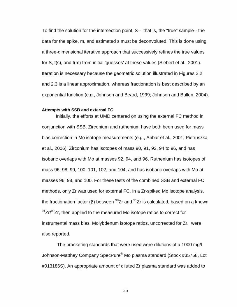
To find the solution for the intersection point, S-- that is, the "true" sample-- the

data for the spike, m, and estimated s must be deconvoluted. This is done using

a three-dimensional iterative approach that successively refines the true values

for S, f(s), and f(m) from initial 'guesses' at these values (Siebert et al., 2001).

Iteration is necessary because the geometric solution illustrated in Figures 2.2

and 2.3 is a linear approximation, whereas fractionation is best described by an

exponential function (e.g., Johnson and Beard, 1999; Johnson and Bullen, 2004).

Attempts with SSB and external FC

Initially, the efforts at UMD centered on using the external FC method in

conjunction with SSB. Zirconium and ruthenium have both been used for mass

bias correction in Mo isotope measurements (e.g., Anbar et al., 2001; Pietruszka

et al., 2006). Zirconium has isotopes of mass 90, 91, 92, 94 to 96, and has

isobaric overlaps with Mo at masses 92, 94, and 96. Ruthenium has isotopes of

mass 96, 98, 99, 100, 101, 102, and 104, and has isobaric overlaps with Mo at

masses 96, 98, and 100. For these tests of the combined SSB and external FC

methods, only Zr was used for external FC. In a Zr-spiked Mo isotope analysis,

the fractionation factor (β) between 90Zr and 91Zr is calculated, based on a known

91Zr/90Zr, then applied to the measured Mo isotope ratios to correct for

instrumental mass bias. Molybdenum isotope ratios, uncorrected for Zr, were

also reported.

The bracketing standards that were used were dilutions of a 1000 mg/l

Johnson-Matthey Company SpecPure® Mo plasma standard (Stock #35758, Lot

#013186S). An appropriate amount of diluted Zr plasma standard was added to

36

the Mo bracketing standard, usually 800 ng/g Mo and 200 ng/g Zr. The acid used

to dilute all samples and standards was 2% nitric acid, mixed using ultrapure

nitric acid and 18mΩ deionized and distilled water. Care was taken to always use

the same batch of acid for dilution of samples and standards, because small

differences in acid strength can create matrix effects.

Using the combination of SSB and external FC methods introduced a

number of technical difficulties. It was found necessary to keep the Zr and

sample Mo signal intensities fairly constant from sample to bracketing standard

(within 5%), and the voltage of Zr had to be no less than 10% of the Mo voltage,

and the ratio of Mo/Zr needed to be fairly high. Deviation from these parameters

resulted in significant automatrix effects, similarly described by Pietruszka et al.

(2006). For the highest-quality data, the voltage of 98Mo (the most abundant

isotope) needed to be higher than 2v, and preferably as high as 5v. This was

generally easily obtained with the 800 ng/g standard solution of Mo.

All published data of Mo isotope ratios in terrestrial materials use 95Mo as

the light isotope in the denominator because it is free of isobaric interference.

Standard delta notation is used:

(2.2) δ98Mosample = 1000*(98/95Mosample/98/95Mostandard)-1)

In sample-standard bracketing, the 98/95Mostandard used to calculate a sample delta

value was the average 98/95Mo of the two bracketing standards. Zirconium was

added to purified samples, standard reference materials, and to the bracketing

standard on the day of analysis. The δ values for a given sample were calculated

37

in two ways: 1) the 'uncorrected' Mo isotope ratios for sample and bracketing

standards would be used to calculate the δ values; 2) the Zr(β)-corrected Mo

isotope ratios for the sample and bracketing standards would be used. Ideally,

the δ values for uncorrected-SSB and the Zr(β)-corrected SSB should be

identical within error.

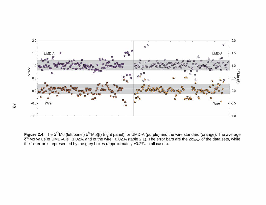
Two pure Mo standard reference materials (Mo wire and UMD-A, a 97Mo-

enriched solution) were analyzed several times during each run. These

standards were measured to high precision during the attempts with SSB and

external FC (Fig. 2.4, Table 2.1). In addition, the data could be compared to

previously measured values for δ97Mo, δ98Mo, and δ100Mo relative to the Mo

plasma standard (Table 2.1; Pietruszka et al., 2006). For the presentation of

these early data, δ97Mo is used, because of the analytical routine that was in use

at the time.

In addition to the solution standards, two different shale samples were

obtained in large quantity to serve as matrix-matched standards for sample

analysis. SDO-1 (Devonian Ohio Shale 1) is a U.S. Geological Survey certified

geochemical reference material, and has known elemental concentrations. Its Mo

concentration is 134 ± 21 µg/g (Kane et al., 1990). In addition, its Mo isotopic

composition has been measured by several other labs. The second standard

shale is NAS (New Albany Shale), which was obtained from the Indiana

Geological Survey, and had a value for Mo concentration of 793 ug/g. Both of

these shales were processed numerous times, and repeatedly measured (Fig.

2.5, Table 2.2). The results for the two shale standards showed initial promise,

38

but data acquired over a long period of time showed that mass-dependent

instrumental fractionation was not being adequately corrected for by sample-

standard bracketing and external FC. Problems primarily arose from the Zr

addition, which were identified by large differences between SSB-δ values from

Zr-fractionation corrected ratios (δ97Mo-β), and SSB-Delta values (δ97Mo),

calculated using an Mo fractionation factor to correct for mass bias. Matrix effects

from a number of sources probably added to the difficulties, although extensive

efforts were made to ensure adequate sample cleanliness. Zirconium addition

may have contributed to matrix effects by changing the sensitivity of Mo in the

plasma. Ultimately, these problems required adoption of a double spike method

to generate data of sufficient precision and accuracy.

39

Figure 2.4: The δ97Mo (left panel) δ97Mo(β) (right panel) for UMD-A (purple) and the wire standard (orange). The average δ97Mo value of UMD-A is +1.02‰ and of the wire +0.02‰ (table 2.1). The error bars are the 2σmean of the data sets, while the 1σ error is represented by the grey boxes (approximately ±0.2‰ in all cases).

40

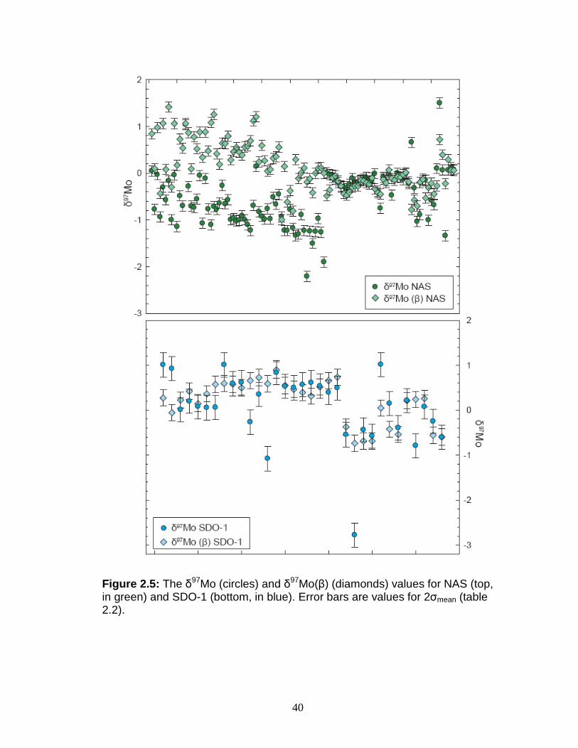
Figure 2.5: The δ97Mo (circles) and δ97Mo(β) (diamonds) values for NAS (top, in green) and SDO-1 (bottom, in blue). Error bars are values for 2σmean (table 2.2).

41

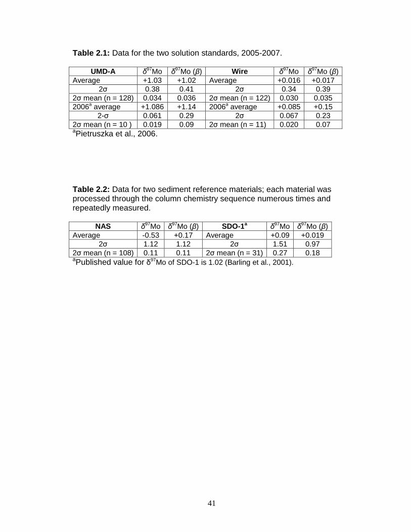
Table 2.1: Data for the two solution standards, 2005-2007.

UMD-A δ97Mo δ97Mo (β) Wire δ97Mo δ97Mo (β) Average +1.03 +1.02 Average +0.016 +0.017

2σ 0.38 0.41 2σ 0.34 0.39 2σ mean (n = 128) 0.034 0.036 2σ mean (n = 122) 0.030 0.035 2006a average +1.086 +1.14 2006a average +0.085 +0.15

2-σ 0.061 0.29 2σ 0.067 0.23 2σ mean (n = 10 ) 0.019 0.09 2σ mean (n = 11) 0.020 0.07 aPietruszka et al., 2006.

Table 2.2: Data for two sediment reference materials; each material was processed through the column chemistry sequence numerous times and repeatedly measured.

NAS δ97Mo δ97Mo (β) SDO-1a δ97Mo δ97Mo (β)

Average -0.53 +0.17 Average +0.09 +0.019 2σ 1.12 1.12 2σ 1.51 0.97

2σ mean (n = 108) 0.11 0.11 2σ mean (n = 31) 0.27 0.18 aPublished value for δ97Mo of SDO-1 is 1.02 (Barling et al., 2001).

42

Preparation and Calibration of a 97Mo-100Mo Double Spike

The 97Mo-100Mo double spike was prepared in collaboration with Drs.

Aaron Pietruszka and Jasper Konter (San Diego State University). Enriched

metal powders of 97Mo (94.2%) and 100Mo (92.6%) were dissolved and diluted

gravimetrically to 6.3378 and 6.5156 µg/g, respectively. These concentrations

were calibrated by mixing the spikes with variable amounts of a Mo-wire

standard prepared gravimetrically to high precision.

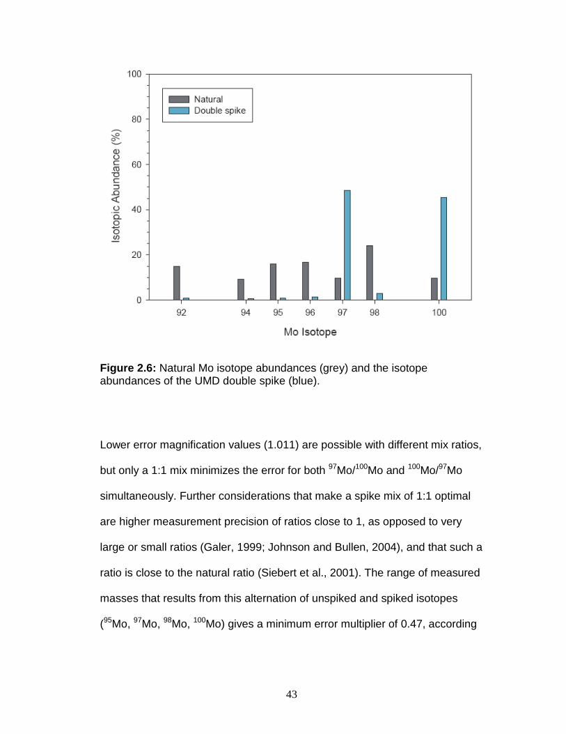
In creating the double-spike, the 97Mo-100Mo isotopes were chosen

because of their relatively low abundance in the Mo mass spectrum (9.55%,

9.63%, respectively; Figure 2.6), which leaves the more abundant 95Mo

(15.89%) and 98Mo (24.23%) isotopes unspiked, and gives the best potential

for high voltages on all ratios during measurement (Johnson and Bullen,

2004). Both 95Mo and 97Mo have no direct isobaric interferences, and 95Mo is

traditionally used as the denominator isotope. 96Mo is avoided in the spike

equations because of potential interferences from both Ru and Zr.

The optimal ratio of the two spikes was determined by assessing the

error magnification that would result from different mixtures, as follows:

(2.3)

−

×

−

÷

−

×

=spmmsspsm

mE100

97

100

97

100

97

100

97

100

97

100

97

100

97)(

Where subscripts m, s, and sp refer to measured, sample, and spike ratios,

respectively. A 1:1 mix results in an error magnification of 1.012 (Figure 2.7).

43

Figure 2.6: Natural Mo isotope abundances (grey) and the isotope abundances of the UMD double spike (blue).

Lower error magnification values (1.011) are possible with different mix ratios,

but only a 1:1 mix minimizes the error for both 97Mo/100Mo and 100Mo/97Mo

simultaneously. Further considerations that make a spike mix of 1:1 optimal

are higher measurement precision of ratios close to 1, as opposed to very

large or small ratios (Galer, 1999; Johnson and Bullen, 2004), and that such a

ratio is close to the natural ratio (Siebert et al., 2001). The range of measured

masses that results from this alternation of unspiked and spiked isotopes

(95Mo, 97Mo, 98Mo, 100Mo) gives a minimum error multiplier of 0.47, according

44

to the formula given by Dodson (1969), as opposed to the error multiplier for

96Mo, 97Mo, 98Mo, 100Mo (0.6):

(2.4) E(m)2 = (∆Mass97, 100)-2 + (∆Mass95, 98)

-2

where the first difference term is for the spike masses, and the second for the

non-spike masses. Double-spike schemes which utilize other spike isotopes

(e.g., 92Mo-98Mo; Wieser and DeLaeter, 2009) can yield lower error multipliers

(0.26), but the measurement program and instrumentation used for this study

would make such a mix more difficult to measure, and prone to greater

measurement errors.

After the optimal spike ratio was found, the best sample:spike ratio was

calculated. It was determined that a small amount of underspiking quickly

leads to large error amplification, but overspiking does not. The main problem

with overspiking appears to be large additions of 95Mo to the mix from the

spike. The ideal mix was found to be around 1:1 spike to sample, which has

an error magnification of 1.28 (Fig. 2.8). Ratios of 0.6 to 4 also have low error

magnification (<1.4). However, a ratio of 4 leads to unacceptably high

contributions to 95Mo from the spike. Ideally, an optimal mix is attained when

>90% of the spike isotopes come from the spike and >90% of the unspiked

isotopes come from the sample (Johnson and Bullen, 2004). This can be

easily demonstrated with an example: for a measured δ98Mo value of 0.1‰,

45

Figure 2.7: Error magnification due to changes in the ratio of 97Mo to 100Mo. The ideal ratio of the two spikes in the final mixed double spike is at the intersection of the two curves, at which point the error magnification is minimized for both curves (1.012). This results in a 1:1 mix of 97Mo to 100Mo.

46

Figure 2.8: Error magnification for sample:spike mixes, where the spike is of the optimal 1:1 composition shown in Fig. 2.7. Vertical lines connect sample:spike ratios to the percent contributions of 95Mo from the spike for that ratio. The horizontal line is an error magnification of 1.4. A sample:spike ratio of 1 is ideal, as this minimizes both the error magnification (1.28) and the contribution to 95Mo from the spike (~5%). A ratio of 2 results in a lower error magnification (1.23) but has a 9.6% contribution to 95Mo from the spike. Arrows indicate direction of, and location where, overspiking and underspiking occur.

47

an error magnification of 1.28 results in a value of 0.128‰, which changes

the value by much less than the external reproducibility. An implication of this

result is that in order to avoid over/underspiking the Mo concentration of the

sample should be known to within 10%.This necessitates a preliminary

concentration measurement for each sample.

The concentration of the final double spike was chosen in order to

minimize the amount of spike needed for most samples, but also avoid having

to measure out very small quantities of spike. Once this was determined, the

two concentrated single spikes were mixed together and diluted to

approximately one liter with ultra-pure, low-molarity nitric acid. All masses

were precisely weighed with a timed evaporation correction and the balance

was calibrated before weighing commenced. The mixed double spike was

allowed to equilibrate for ~36 hours.

The composition and concentration of the double spike was

determined by creating a series of mixes with varying proportions of double

spike and wire standard with a known concentration of 1.922 µg/g (Table 2.3).

Teflon beakers were carefully weighed 5 times, and then aliquots of the wire

standard and double spike were added (separately) and weighed accurately

to 5 decimal places by timed evaporation correction. These mixes covered a

range from pure double spike to pure wire (Fig. 2.9). The Mo concentration of

the double spike was determined by calculating its concentration in each mix

using isotope dilution calculations, treating the wire standard as the ‘spike’

and the double spike as the ‘unknown’. Thus the Mo concentration of the

48

double spike was determined to be 29.3944 (± 0.035, 2 s.d.). The

fractionation-corrected composition of the final double spike is given in Table

2.4. This was determined by correcting the measured ratios for each isotope

pair of each mix, to the expected value of the ratio based on the proportions

in the mix and the previously established compositions of the single spikes

and the wire standard. The data acquisition routine designed to perform the

Mo isotope measurements using the UMD Nu-Plasma MC-ICP-MS is shown

in Table 2.5. The three ratios used are 95Mo/98Mo, 97Mo/98Mo, and

100Mo/98Mo. The geometric approach (described on pages 43-45, illustrated in

Figures 2.2 and 2.3) was refined specifically for Mo by Siebert et al. (2001).

The Siebert et al. solution requires nested iterations to refine initial the

starting values for coefficients for natural and instrumental fractionation, and

sample and standard values, until there is convergence upon a "true" value

for the sample isotopic composition. This approach was converted to a

MATLAB program by Jasper Konter. This program performs 1000 nested

iterations and incorporates the 1 s.e. measurement errors for each ratio. The

'assumed' parameters used are the ratios for the wire standard, and

estimates of the degree of natural and instrumental fractionation (0.5 for

both).

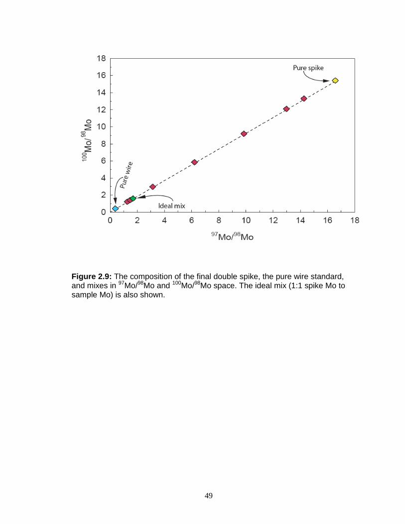
49

Figure 2.9: The composition of the final double spike, the pure wire standard, and mixes in 97Mo/98Mo and 100Mo/98Mo space. The ideal mix (1:1 spike Mo to sample Mo) is also shown.

50

Table 2.3: Fractionation-corrected ratios for the mixes of double spike and Mo wire. Mix D is the ideal sample:spike ratio. The instrumental background noise has been subtracted from the ratios. The 1 s.e. is the instrumental error on that ratio during measurement.

Mix (spike µg:wire µg)

92/98 1 s.e. 94/98 1 s.e. 95/98 1 s.e. 96/98 1 s.e. 97/98 1 s.e. 100/98 1 s.e.

Pure wire 0.52901 2.8E-05 0.34680 1.2E-05 0.61261 1.6E-05 0.65556 9.8E-06 0.38619 4.1E-06 0.41836 7.6E-06 Mix A (0.7) 0.58830 1.7E-05 0.36731 7.0E-06 0.63526 1.0E-05 0.67197 8.3E-06 1.27031 9.2E-06 1.21711 1.7E-05 Mix B (0.9) 0.58376 3.7E-06 0.36434 1.9E-06 0.63035 3.0E-06 0.66918 3.0E-06 1.48045 6.3E-06 1.41333 7.6E-06 Mix D (1.1) a 0.57901 5.5E-06 0.36123 2.8E-06 0.62538 3.4E-06 0.66581 3.0E-06 1.68754 6.2E-06 1.60699 5.8E-06 Mix E (2.5) 0.54462 5.6E-06 0.33916 3.5E-06 0.58999 3.9E-06 0.64136 4.6E-06 3.13855 1.8E-05 2.97007 2.1E-05 Mix F (6.9) 0.47765 6.3E-06 0.29520 3.5E-06 0.51855 5.9E-06 0.59353 7.2E-06 6.21223 5.9E-05 5.85091 7.6E-05 Mix G (17.2) 0.40669 7.0E-06 0.24614 4.8E-06 0.43827 7.8E-06 0.53759 6.8E-06 9.84649 1.3E-04 9.18503 1.2E-04 Mix H (43.0) 0.33888 7.8E-06 0.20120 6.6E-06 0.36544 7.4E-06 0.48834 1.1E-05 12.98074 2.9E-04 12.09771 2.3E-04 Mix J (73.9) 0.31077 1.0E-05 0.18265 8.0E-06 0.33537 9.6E-06 0.46784 9.3E-06 14.26339 3.9E-04 13.29812 3.7E-04 Pure D.S. 0.26204 1.4E-05 0.14991 8.7E-06 0.28251 1.4E-05 0.43108 1.1E-05 16.57465 3.8E-04 15.41567 3.6E-04 aIdeal mix

51

Table 2.4: Isotopic composition of the single spikes and the final double spike. Mo isotope 97Mospike 9xMo/98Mo

in 97Mospikea

100Mospike 9xMo/98Mo in 100Mospike

a

97Mo/100Mo 9xMo/98Mo in DSb

92Mo 0.00189 0.05743 0.01145 0.48368 0.00758 0.26204 94Mo 0.00175 0.05282 0.00622 0.26140 0.00435 0.14991 95Mo 0.00448 0.12781 0.01088 0.45089 0.00821 0.28251 96Mo 0.01214 0.34425 0.01211 0.49649 0.01246 0.43108 97Mo 0.94203 26.52343 0.00761 0.31138 0.048463 16.57465 98Mo 0.03442 1 0.02379 1 0.02927 1 100Mo 0.00328 0.09079 0.92794 36.89286 0.45350 15.41567

a Measured ratios internally fractionation corrected for β = 1.7178. b Double spike

Table 2.5: The Faraday detector arrangement for an Mo isotope measurement. The instrument measures each requested isotope ratio 15 times per block, for a total of 4 blocks, with zeroes at half-mass after every block. The program centers the axial peak (Ax) before each block. A gain calibration was run on each day that measurements were made. After a minimum two hours of warm-up time, the instrument was tuned to at least 2v on 98Mo for all measurements. Zirconium and Ru, which overlap the Mo mass spectrum, were monitored on one isotope each (90 and 99, respectively) to ensure that no direct interferences were occurring from these elements. All ratios were measured to internal precision better than 0.01% (2σ). Detector H6 H5 H4 H3 H2 H1 Ax L1 L2 L3 L4 L5

Zero 1 99 98 97 -- 96 -- 95 -- 94 93 92 91

Zero 2 97.55 96.55 95.55 -- 94.55 -- 93.55 -- 92.55 91.55 90.55 89.55

Cycle 1 99.55 98.55 97.55 -- 96.55 -- 95.55 -- 94.55 93.55 92.55 91.55

52

Long term result for standards with the double spike method

A summary of the data acquired for our in-house reference materials

illustrates the performance of the double spike over the two years of its use.

The baseline for double spike measurements is a mix of the plasma standard

and the double spike. This is measured every session, and long-term

reproducibility of its delta value is, as expected, very high (Table 2.6). This

procedure also provides a fractionation-corrected 98/95Mo ratio for the

standard. Delta values were calculated by comparing the reduced sample

98/95Mo ratio to the 98/95Mo ratio for an in-house Johnson-Matthey Company

SpecPure® Mo plasma standard (Stock #35758, Lot #013186S). The

SpecPure® Mo plasma standard is frequently used in the literature as the

standard reference to calculate a delta value for seawater (+2.3‰, Siebert et

al., 2003).

This procedure provided an additional check on long-term instrument

performance with respect to Mo isotopes, through comparison of δ98Mo

values for the Mo standard. Similarly, a mix of a proposed NIST Mo solution

standard (Table 2.7) and the double spike was measured in two different

sessions a year apart, and have very high reproducibility (Table 2.8).

The performance of the Nu- plasma is monitored in part by an internal

fractionation correction measured with an the Mo plasma standard. An

internal fractionation factor is calculated for 98/95Mo which is then used to

calculate corrected values for 92/95Mo, 97/95Mo, and 100/95Mo. Epsilon values

are then calculated for these fractionation corrected ratios. While the value

that is used as the standard in the epsilon equation is arbitrary, the

53

expectation exists that the instrument be able to obtain results within half an

epsilon unit of the nominal value. If this is not the case, additional tuning is

performed.

In addition to SDO-1 and NAS, multiple aliquots of Fairhaven sediment

and a Mediterranean sapropel sample (969D 4H-2, 131) have been

processed. Long-term external reproducibility of two in-house rock reference

standards is ±0.2‰ for δ98Mo at the 2σ level (Fig. 2.10, table 2.9). Five

separate analyses of the Fairhaven sample yield variance of 15.5 ±0.1 µg/g in

concentration and δ98Mo +0.94‰ ±0.09 (2σ). One of the rock standards,

USGS SDO-1, has published Mo isotope values of δ98Mo +1.16‰ ± 0.1 (2σ)

and +1.2 ± 0.3 (2σ) (Wasylenki et al., 2008; Poulson-Brucker et al., 2009).

Our δ98Mo value of +0.88‰ ± 0.19 (2σ, n = 54) is offset to a slightly lower

value by ~0.3‰, which is just within the published errors. The offset, if real,

could be due to isotopic differences between batches of SpecPure® Mo, or,

more unlikely, to heterogeneity in the SDO-1 standard. Inter-lab comparison

of results is stifled by the lack of a true isotopic standard, and the differences

in isotopic values of a rock standard emphasizes the need to establish a

bona-fide isotopic reference material.

The results for these reference materials appear to have better

reproducibility over the relatively short periods of time, for example in a three-

day measurement session, as opposed to month to month. This can be seen

in Fig. , where clusters of analyses with similar δ98Mo values are apparent.

These clusters often are indicative of data collected within a short span of

time.

54

Table 2.6: Data for measurements of the mix of double spike plus Mo plasma standard. 1 s.e. are instrumental errors. All measurements made with the Apex unless otherwise noted. The average δ98Mo is -0.07‰ (±0.05, 2σmean).

aApril 29, 2008, bMay 14, 2008, cJune 2, 2009, dJune 4, 2009, eJuly 8, 2009, fJuly 31, 2009, gAug 14, 2009 (Aridus), hSeptember 7, 2009 98/95Mo to calculate δ98Mo: 1.524905

100/98 1 s.e. 97/98 1 s.e. 95/98 1 s.e.

95/98 (reduced) δ

98Mo Ds/Psa 1.84702 3.2E-5 1.84331 2.2E-5 0.58847 1.1E-5 0.65596 -0.28 Ds/Ps 1.84860 3.1E-5 1.84243 2.2E-5 0.58747 7.7E-6 0.65568 0.16 Ds/Ps 1.84893 3.7E-5 1.84251 1.6E-5 0.58742 7.5E-6 0.65572 0.09 Ds/Ps 1.84508 3.7E-5 1.84371 4.0E-5 0.58926 1.6E-5 0.65600 -0.34 Ds/Psb 1.83860 1.1e-4 1.84727 7.1e-5 0.59234 5.0e-5 0.65571 0.11 Ds/Psc 1.86194 3.8E-5 1.86481 2.0E-5 0.58994 1.4E-5 0.65581 -0.04 Ds/Ps 1.86223 4.0E-5 1.86470 2.3E-5 0.58982 1.8E-5 0.65582 -0.06 Ds/Ps 1.86205 3.0E-5 1.86473 1.6E-5 0.58989 1.3E-5 0.65582 -0.06 Ds/Ps 1.86220 4.7E-5 1.86464 2.3E-5 0.58988 1.8E-5 0.65591 -0.20 Ds/Ps 1.86254 4.1E-5 1.86455 2.1E-5 0.58974 1.5E-5 0.65591 -0.19 Ds/Ps 1.86267 7.8E-5 1.86444 3.7E-5 0.58961 3.3E-5 0.65583 -0.08 Ds/Ps 1.86140 2.7E-5 1.86510 1.8E-5 0.59018 1.2E-5 0.65576 0.03 Ds/Psd 1.86336 4.0E-5 1.86425 2.0E-5 0.58931 1.6E-5 0.65582 -0.07 Ds/Ps 1.86413 5.0E-5 1.86382 2.6E-5 0.58899 2.5E-5 0.65591 -0.2 Ds/Ps 1.86476 2.4E-5 1.86359 1.7E-5 0.58864 1.0E-5 0.65581 -0.05 Ds/Ps 1.86350 3.1E-5 1.86442 1.4E-5 0.58937 1.0E-5 0.65591 -0.2 Ds/Pse 1.86327 5.2E-5 1.86302 4.8E-5 0.58891 2.3E-5 0.65574 0.07 Ds/Ps 1.86090 6.9E-5 1.86474 4.0E-5 0.59025 2.3E-5 0.65578 -0.01 Ds/Ps 1.86324 7.3E-5 1.86373 4.3E-5 0.58908 2.5E-5 0.65565 0.20 Ds/Ps 1.85682 8.4E-5 1.85549 6.3E-5 0.58872 3.3E-5 0.65567 0.17 Ds/Ps f 1.85206 5.2E-5 1.85458 4.5E-5 0.59013 2.3E-5 0.65582 -0.06 Ds/Ps 1.85755 3.9E-5 1.85369 3.3E-5 0.58808 1.6E-5 0.65589 -0.18

Ds/Psg 1.86682 1.7E-4 1.85679 1.6E-4 0.58594 1.2E-5 0.65588 -0.15 Ds/Ps 1.86948 5.0E-5 1.85929 4.0E-5 0.58584 7.2E-6 0.65590 -0.18 Ds/Ps 1.87022 2.1E-5 1.86014 2.3E-5 0.58583 8.0E-6 0.65587 -0.14

Ds/Psh 1.86741 4.3E-5 1.86165 2.3E-5 0.58718 1.8E-5 0.65580 -0.04 Ds/Ps 1.86742 4.8E-5 1.86188 2.4E-5 0.58724 2.0E-5 0.65581 -0.06 Ds/Ps 1.86764 4.7E-5 1.86133 2.4E-5 0.58717 1.1E-5 0.65584 -0.09

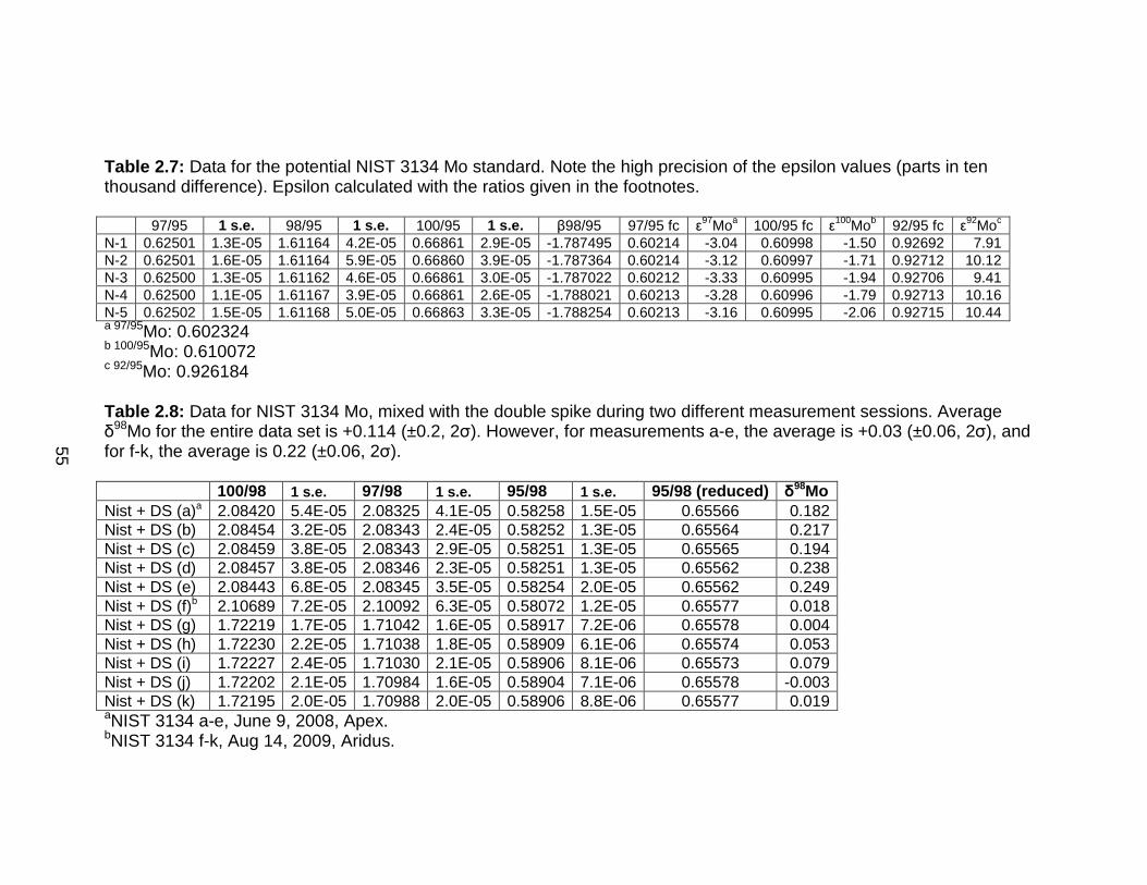
55

Table 2.7: Data for the potential NIST 3134 Mo standard. Note the high precision of the epsilon values (parts in ten thousand difference). Epsilon calculated with the ratios given in the footnotes. 97/95 1 s.e. 98/95 1 s.e. 100/95 1 s.e. β98/95 97/95 fc ε

97Moa 100/95 fc ε100Mob 92/95 fc ε

92Moc

N-1 0.62501 1.3E-05 1.61164 4.2E-05 0.66861 2.9E-05 -1.787495 0.60214 -3.04 0.60998 -1.50 0.92692 7.91 N-2 0.62501 1.6E-05 1.61164 5.9E-05 0.66860 3.9E-05 -1.787364 0.60214 -3.12 0.60997 -1.71 0.92712 10.12 N-3 0.62500 1.3E-05 1.61162 4.6E-05 0.66861 3.0E-05 -1.787022 0.60212 -3.33 0.60995 -1.94 0.92706 9.41 N-4 0.62500 1.1E-05 1.61167 3.9E-05 0.66861 2.6E-05 -1.788021 0.60213 -3.28 0.60996 -1.79 0.92713 10.16 N-5 0.62502 1.5E-05 1.61168 5.0E-05 0.66863 3.3E-05 -1.788254 0.60213 -3.16 0.60995 -2.06 0.92715 10.44 a 97/95Mo: 0.602324 b 100/95Mo: 0.610072 c 92/95Mo: 0.926184 Table 2.8: Data for NIST 3134 Mo, mixed with the double spike during two different measurement sessions. Average δ98Mo for the entire data set is +0.114 (±0.2, 2σ). However, for measurements a-e, the average is +0.03 (±0.06, 2σ), and for f-k, the average is 0.22 (±0.06, 2σ). 100/98 1 s.e. 97/98 1 s.e. 95/98 1 s.e. 95/98 (reduced) δ98Mo Nist + DS (a)a 2.08420 5.4E-05 2.08325 4.1E-05 0.58258 1.5E-05 0.65566 0.182 Nist + DS (b) 2.08454 3.2E-05 2.08343 2.4E-05 0.58252 1.3E-05 0.65564 0.217 Nist + DS (c) 2.08459 3.8E-05 2.08343 2.9E-05 0.58251 1.3E-05 0.65565 0.194 Nist + DS (d) 2.08457 3.8E-05 2.08346 2.3E-05 0.58251 1.3E-05 0.65562 0.238 Nist + DS (e) 2.08443 6.8E-05 2.08345 3.5E-05 0.58254 2.0E-05 0.65562 0.249 Nist + DS (f)b 2.10689 7.2E-05 2.10092 6.3E-05 0.58072 1.2E-05 0.65577 0.018 Nist + DS (g) 1.72219 1.7E-05 1.71042 1.6E-05 0.58917 7.2E-06 0.65578 0.004 Nist + DS (h) 1.72230 2.2E-05 1.71038 1.8E-05 0.58909 6.1E-06 0.65574 0.053 Nist + DS (i) 1.72227 2.4E-05 1.71030 2.1E-05 0.58906 8.1E-06 0.65573 0.079 Nist + DS (j) 1.72202 2.1E-05 1.70984 1.6E-05 0.58904 7.1E-06 0.65578 -0.003 Nist + DS (k) 1.72195 2.0E-05 1.70988 2.0E-05 0.58906 8.8E-06 0.65577 0.019 aNIST 3134 a-e, June 9, 2008, Apex. bNIST 3134 f-k, Aug 14, 2009, Aridus.

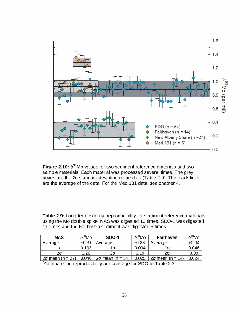
56

Figure 2.10: δ98Mo values for two sediment reference materials and two sample materials. Each material was processed several times. The grey boxes are the 2σ standard deviation of the data (Table 2.9). The black lines are the average of the data. For the Med 131 data, see chapter 4. Table 2.9: Long-term external reproducibility for sediment reference materials using the Mo double spike. NAS was digested 10 times, SDO-1 was digested 11 times,and the Fairhaven sediment was digested 5 times.

NAS δ98Mo SDO-1 δ98Mo Fairhaven δ98Mo Average +0.31 Average +0.88a Average +0.94

1σ 0.103 1σ 0.094 1σ 0.046 2σ 0.20 2σ 0.19 2σ 0.09

2σ mean (n = 27) 0.040 2σ mean (n = 54) 0.025 2σ mean (n = 14) 0.024 aCompare the reproducibility and average for SDO to Table 2.2.

57

Column chemistry and sample preparation

Column Chemistry

A two-column chromatographic separation consisting of anion-

exchange and cation-exchange steps, was used to purify samples containing

complex matrices of organic matter, clay and silicate (Pietruszka et al., 2006).

The anion chemistry accomplishes stepwise separation of such matrix

elements as Fe3+, Al, K, and Zr from retained Mo, while the cation column

retains the matrix elements and does not retain Mo in the correct acid

strength. Initially, the Teflon columns used for anion separate were 34 cm

long with a 0.6 cm i.d. The teflon columns used for cation separation were 12

cm long with a 0.6 cm i.d. Each type of column was fitted with a frit and Teflon

dripper. These columns held ~10 ml and ~3.5 ml of resin, respectively. To

ensure low blank, the anion resin was batch-cleaned thoroughly prior to use,

using 8M HNO3, 6M HCl, and 1M HCl, sequentially, with 2 rinse steps in

distilled de-ionized water between each acid. A second cleaning of the anion

resin was performed in the column just prior to sample addition by rinsing with

three different strengths of HCl. Acid strengths were checked at room

temperature using a densitometer.

To ensure complete separation from other elements and high Mo yield

off the anion column (to avoid fractionation on the column), large volumes of

acid were used during the processing (e.g., 120 ml of 1M HCl and 50 ml of

5M HNO3 were used to elute Mo). This method was altered after it was found

that almost all the Mo is eluted with the first 30 ml of 1M HCl, making the use

of 5M HNO3 as an Mo eluent superfluous (Fig 2.11 and table 2.10). The anion

58

resin was discarded after each sample, but the cation resin was cleaned with

250 ml of 6M HCl, and reused. Using this procedure, a set of 6 samples took

more than a week to prepare for analysis, because of the long time each acid

took to drip through the column, and the time needed to reduce 170 ml of

eluent to dryness on a 90°C hot plate, in order to pr oceed to the next step.

Eventually, the need to process a large number of samples in shorter

time necessitated changing the column chemistry. The size of column used

was the main alteration; the overall sequence of acids was not changed. In

lieu of the Teflon columns, Biorad polyproplyene (Poly-prep™) disposable

columns with a 2 cm resin bed and 10 ml sample reservoir and porous 20 µm

hydrophilic polymer frit were employed for both the anion and cation

chemistry. Accordingly, the volumes of acid needed to achieve a quantitative

Mo yield were much less (Tables 2.11 and 2.12). The small quantity of resin

used (~2-3 ml) meant that saturating the resin with ions might be a problem.

However, the small sample quantities that were generally dissolved and

passed through the column were well under the resin capacity

A second change was the addition of a third column. This last column

was a scaled-down version (1/10 the size) of the starting anion column, and

its purpose was to remove the last traces of Fe, Zr, and other elements

remaining after the cation separation. The sequence of acids used to

accomplish the separation was not changed significantly in the 3 column

procedure compared to the two-column procedure . The time required for the

59

three-column process was ~4 days from start to finish, and up to 20 samples

could be processed simultaneously.

After the Mo was separated and dried, a small amount of aqua regia

was added. This was done to destroy any organic residue that may have

been added to the sample from the resin (Pietruszka and Reznick, 2008).

Just prior to analysis, the separated Mo was dissolved in an appropriate

amount of 2% nitric acid and refluxed on a hot plate. Digestion and column

blanks were assessed by passing a known amount of 97Mo spike through the

digestion and column separation chemistry. Blanks for the 3-column

chemistry ranged between 2 and 6 ng Mo, comprising less than 1% of the

total Mo for any sediment samples.

60

Figure 2.11: Test of Mo elution in the anion column. The test used 0.01452g of NAS, resulting in 8.4216 ug of Mo in the sample. Cuts 1-12 are 1M HCl, while cuts 13-17 were 5M HNO3. Each cut was 10 ml.

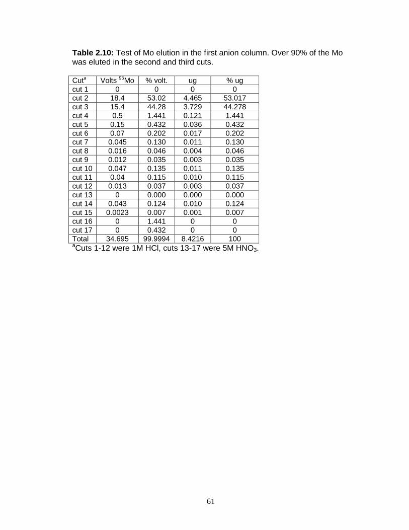
61

Table 2.10: Test of Mo elution in the first anion column. Over 90% of the Mo was eluted in the second and third cuts. Cuta Volts 95Mo % volt. ug % ug cut 1 0 0 0 0 cut 2 18.4 53.02 4.465 53.017 cut 3 15.4 44.28 3.729 44.278 cut 4 0.5 1.441 0.121 1.441 cut 5 0.15 0.432 0.036 0.432 cut 6 0.07 0.202 0.017 0.202 cut 7 0.045 0.130 0.011 0.130 cut 8 0.016 0.046 0.004 0.046 cut 9 0.012 0.035 0.003 0.035 cut 10 0.047 0.135 0.011 0.135 cut 11 0.04 0.115 0.010 0.115 cut 12 0.013 0.037 0.003 0.037 cut 13 0 0.000 0.000 0.000 cut 14 0.043 0.124 0.010 0.124 cut 15 0.0023 0.007 0.001 0.007 cut 16 0 1.441 0 0 cut 17 0 0.432 0 0 Total 34.695 99.9994 8.4216 100 aCuts 1-12 were 1M HCl, cuts 13-17 were 5M HNO3.

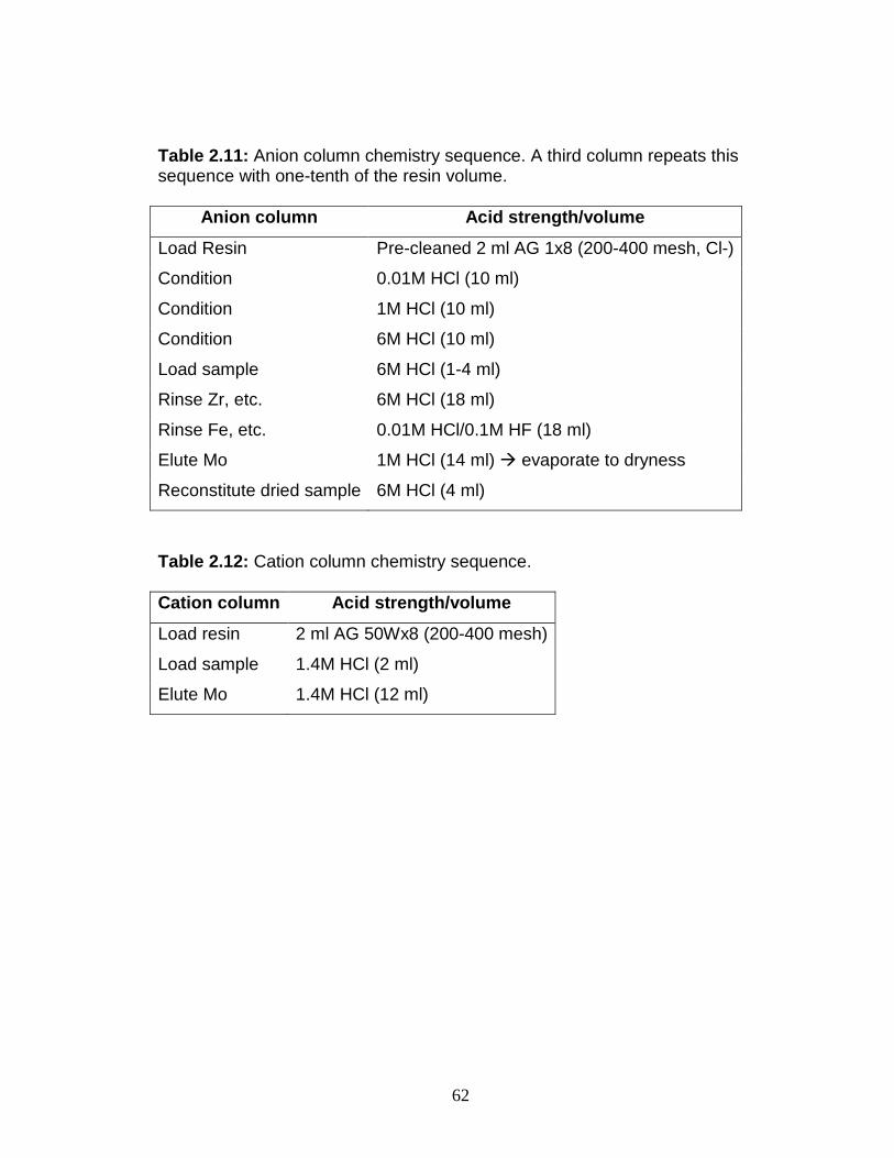
62

Table 2.11: Anion column chemistry sequence. A third column repeats this sequence with one-tenth of the resin volume.

Anion column Acid strength/volume

Load Resin Pre-cleaned 2 ml AG 1x8 (200-400 mesh, Cl-)

Condition 0.01M HCl (10 ml)

Condition 1M HCl (10 ml)

Condition 6M HCl (10 ml)

Load sample 6M HCl (1-4 ml)

Rinse Zr, etc. 6M HCl (18 ml)

Rinse Fe, etc. 0.01M HCl/0.1M HF (18 ml)

Elute Mo 1M HCl (14 ml) evaporate to dryness

Reconstitute dried sample 6M HCl (4 ml)

Table 2.12: Cation column chemistry sequence.

Cation column Acid strength/volume

Load resin 2 ml AG 50Wx8 (200-400 mesh)

Load sample 1.4M HCl (2 ml)

Elute Mo 1.4M HCl (12 ml)

63

Sediment sample preparation

Sediment samples were prepared by grinding to a fine powder in a

ceramic mortar. Organic-rich powders were combusted at 500°C in a muffle

furnace for 5-6 hours. It was determined that Mo is not lost during the

combustion process and does not alter the isotopic composition of samples,

based on comparative tests of combusted and non-combusted rock

standards. After combustion, ~200-500 mg of sample were weighed into 15

ml Teflon Savillex screw-cap beakers, and a 97Mo-100Mo double spike solution

(29.39 µg/g Mo in 2% nitric acid) was weighed and added. Digestion

proceeded sequentially at 90-120° on a hotplate, using first aqua regia, then

HNO3 plus concentrated HF, and lastly concentrated HCl, drying the sample

between each step. The dissolution steps were repeated until the solution in

the beaker was clear and free of visible particles. All acids except for HF

were quartz distilled. The HF was Seastar™ Baseline®, which typically has

Mo impurities of <5 pg/g.

Preparation of water samples

Due to the saline nature of the water samples that were collected from

the Chesapeake Bay (Chapter 3), additional treatment was required before

the samples could be processed via the standard column sequence (T. Dahl,

personal communication). Chelating resin (Biorad Chelex-100) was stirred

with 1 L of acidified sample, plus spike, for 24 hours (Table 2.13). In the case

of the Susquehanna River, 5 L of water was used in order to obtain a

64

maximum amount of Mo for analysis. The resin was decanted, and Mo and

other metals were eluted using NH4OH. The sample was then passed through

the standard column chemistry, as already described. A test of the sample

yield revealed that the method was successful at removing close to 97% of

the spike and sample Mo from the water, and that 90% of this Mo could then

be retrieved from the chelating resin. The blank for one liter of distilled water

was 0.22 µg, or approximately 4% of the sample Mo for the estuarine

samples, but ~20% of the Mo in the river water.

Water samples from the Chesapeake Bay were collected in 1-gallon

HDPE jugs by the Maryland Department of Natural Resources, during a

research cruise August 18-19, 2008. The jugs were purchased sealed and

filled with distilled water. Aboard ship, the distilled water was emptied, the jug

was filled and emptied 3 times with the ambient water, and then filled and

closed. It was determined that acid-leaching the jugs prior to the water

collection was unnecessary, because there was no measurable Mo in the

distilled water, or in a sample of 5% HNO3 used to leach the plastic for ~24

hours. These two assessments were made using a Thermo E2 single-

collector ICP-MS.

Water from the Susquehanna River was collected by the author on

March 20, 2009, below the Conowingo Dam outflow. A 5-gallon HDPE carboy

was used; this carboy was acid-leached for 4 days in 5% HNO3, because it

had previously been used for water sampling. The carboy was filled by

65

wading into the river, submerging the jug and emptying it 3 times, and then

filling it.

Table 2.13: Chelating Resin chromatography sequence for water samples.

Chelating Chemistry Treatment

Acidify 1L sample to pH 1 Conc. HNO3

Add double spike Low heat, equilibrate 36 hours

Buffer solution to pH 4.8-5.5 CH3COONH4

Add 6 ml Chelex-100 Stir 24 hours, then decant resin to a clean column

Elute Mo (and other metals) 4M NH4OH (50 ml stepwise)

Dry, redissolve, proceed to anion column

2-4 ml 6M HCl

66

Chapter 3: Century-long record of Mo isotopic composition in sediments of a seasonally anoxic estuary (Chesapeake Bay) 2

Abstract A double-spike method was used to obtain Mo isotope data for

sediments and waters of the seasonally anoxic Chesapeake Bay, and its

primary tributary, the Susquehanna River. The dissolved Mo distribution in the

estuary is non-conservative, reflecting minor Mo loss to the sediments,

although removal of Mo to the sediments does not have a large influence on

the isotopic composition of the water column. The δ98Mo of dissolved Mo in

most of the estuary is dominated by seawater. Six samples with salinity >15

have an average δ98Mo = +2.17‰ (± 0.12), which agrees well with a δ98Mo

value for the CASS-4 seawater standard of +2.23‰. A single sample of

Susquehanna River water has a δ98Mo of +1.02‰, consistent with recent

findings of positive δ98Mo in rivers worldwide. Susquehanna river sediments,

in contrast, have δ98Mo ~ -0.1‰. The difference between the river water and

sediment values implies that isotopic fractionation occurs within the river

basin. The δ98Mo values for estuarine sediments are offset from values in the

overlying water. Most samples deposited before 1925 have δ98Mo less than

0‰, similar to the Susquehanna sediments. Subsequently, there is an

increase in the variability of δ98Mo, with values ranging up to +0.8‰. The

transition to increased variability coincides with the onset of authigenic Mo

deposition, which was previously attributed to escalating summertime anoxia.

2This chapter has been published in Earth and Planetary Science Letters as Scheiderich, K., Helz, G.R. and Walker, R.J., 2010.

67

Authigenic Mo concentrations correlate poorly with δ98Mo in core samples,

suggesting that independent mechanisms influence the two parameters.

Authigenic Mo concentrations may be controlled by shifting pore water H2S

levels, while δ98Mo may be primarily affected by annual variations in Mn

refluxing.

Introduction Dissolved Mo in seawater, present almost entirely as MoO4

2-, has an

isotopic composition (δ98Mo) that is believed to be as much as 2‰ heavier

than Mo delivered from continental sources, such as clastic sediments and

igneous rocks (Barling et al., 2001; Siebert et al., 2003). Manganese

oxyhydroxides (henceforth MnOx) are a major sink for Mo in oxygenated

seawater (Bertine and Turekian, 1973), and it has been shown that the Mo

adsorbed onto MnOx is isotopically light relative to dissolved MoO42- in the

source solution (Barling et al., 2001; Barling and Anbar, 2004; Siebert et al.,

2003; Wasylenki et al., 2008). This supports the idea that fractionation of Mo

isotopes during adsorption to MnOx is primarily responsible for the heavy

isotopic composition of seawater (Barling et al., 2001; Barling and Anbar,

2004; Siebert et al., 2003).

This simple model has been used to interpret the oxygenation histories

of ancient and modern oceans (e.g., Poulson et al., 2006; Wille et al., 2007),

and freshwater systems (e.g., Malinovsky et al., 2007). Formation of MnOx

from dissolved Mn(II) requires a high oxidation potential and is, therefore,

believed to have always required free O2. Consequently, the history of free O2

68

availability in the ocean can be potentially assessed with the aid of Mo

isotopes in sedimentary rocks (Arnold et al., 2004; Pearce et al., 2008; Wille

et al., 2007).

Complicating such interpretations is the discovery that authigenic Mo

deposited in suboxic (O2 < 10µM) environments is 1 to 2‰ lighter than

seawater (Siebert et al., 2006). Since MnOx is not deposited under suboxic

conditions, at least one additional process for selectively removing light Mo

isotopes from seawater must exist. This process probably contributes to the

modern, heavy δ98Mo value of seawater, and will have contributed to past

seawater δ98Mo values.

Fractionation during thiomolybdate formation is a second process that

might influence δ98Mo values in sediments from suboxic zones. Quantum

mechanical calculations indicate that negative equilibrium isotopic

fractionations on the order of -2 to -5‰ occur in the presence of sulfide, and

could be detected if removal of Mo from seawater were incomplete (Tossell,

2005). In support of this idea, fractionation of up to -3‰ between dissolved

and particulate Mo is observed under mildly sulfidic, but euxinic conditions in

the Black Sea (Neubert et al., 2008).

The potential for using Mo isotopes to monitor paleoredox conditions

may also be further complicated by the report of isotopic compositions

heavier than 0‰ in a number of rivers (Archer and Vance, 2008). It has been

assumed that the continents deliver material with Mo isotopic compositions

close to 0‰, but this now appears to be overly simplistic. Generation of

69

isotopically heavy Mo in seawater can no longer be assumed to be a result of

processes wholly internal to the ocean; continental weathering regimes are

probably contributing through as-yet unidentified mechanisms. Therefore, to

better understand Mo isotopes in the ocean, isotopic fractionation processes

within estuaries and river basins must be investigated.

Estuaries represent the geochemical transition zone between river

basins and the ocean. It is unknown what Mo isotopic fractionation processes

might occur in estuaries, and how such processes might affect the isotopic

composition of the ocean. This study provides the first survey of Mo isotopes

in both the sediments and waters of an estuarine system. We report Mo

concentrations and isotopic data from one of the largest and most extensively

studied North American estuaries, Chesapeake Bay, located on the east

coast of the United States (Fig. 3.1). During the 20th century, Chesapeake

Bay underwent a change from a well oxygenated to a seasonally anoxic

estuary (Adelson et al., 2001; Cronin and Vann, 2003; Hagy et al., 2004;

Zimmermann and Canuel, 2002), making the historic pattern of Mo isotopes

in Chesapeake Bay sediments of particular interest.

Sample descriptions

Water samples

Eight water samples from six stations in the main stem of the Chesapeake

Bay were obtained (Fig. 3.1). The samples were collected August 12-13,

2008 by the Maryland Department of Natural Resources. At all stations, water

was collected in distilled water leached 1-gallon HDPE jugs at mid-depth

70

(Table 3.1). At the two end-member stations, water was also collected within

one meter of the bottom. Temperature, pH, salinity, and dissolved O2

measurements were taken at depth during sampling. All Mo concentrations

were determined the day after sampling, and Mo for isotopic composition

measurements was processed 3-4 months later. No reagents were added

before processing began. Water from the Susquehanna River was obtained

March 19, 2009, in an acid-leached 5-gallon HDPE carboy. The water was

collected from shore, below the outflow of the Conowingo Dam. Processing

for Mo isotopes proceeded on the same day.

71

Figure 3.1: Chesapeake Bay and environs. Site locations for Chesapeake Bay water samples (blue circles), and sediments are shown. The green triangle is the location of both the Susquehanna River water sample and sediments. Other symbols are (North to South): orange diamonds- Baltimore Harbor; grey circle- Core RD; purple triangle- Depth Traverse; grey diamond- Core 55; grey square-- Fairhaven; green square- PC-6. The upper left inset map provides location of Chesapeake Bay in the state of Maryland.

72

Sediment samples

A total of forty sediment samples from seven sites (Fig. 3.1) in the

Chesapeake Bay were analyzed for their Mo concentration and isotopic

composition. All sediments are from archived collections that have been the

subject of previous publications (Dolor et al., 2009; Helz et al., 1985a, 1985b;

Marcantonio et al., 2002; Officer et al., 1984; Sinex and Helz, 1981; Sinex

and Helz, 1982; Zimmermann and Canuel, 2002), and additional information

on the sites is available in the Electronic Supplement. The data are intended

to establish the historical extent of seasonal anoxia by analyzing samples

from two long cores (Table 3.2) covering the entire 20th century, and

supplementing the core data with small sample sets (Table 3.3) representing

sources and processes within and around the Bay.

73

Table 3.1: Data for Chesapeake Bay water samples, Susquehanna River water, and a seawater standard.

Station ID Lat./Long. Sample depth (meters)

Salinity Temp. (°C)

Diss. O 2 (mg/L)

pH Mo (µg/L) δ98Mo

CB 3.1 (intermediate)a Gunpowder Neck

39.14'54º/ 76.14'16º 7 11.6 25.3 2.2 7.4 3.07 1.81

CB 3.1 (bottom)b Gunpowder Neck

39.14'54º/ 76.14'16º 13 15.9 25 0.2 7.4 4.35 2.25

CB 3.2 (intermediate) Swan Point

39.9'48º/ 76.18'22º 3 8.7 24.8 5.6 8.1 2.36 1.99

CB 3.3 (intermediate) Bay Bridge

39.59'42º/76.21'34º 17 19.7 25.1 0.2 7.4 5.57 2.26

CB 4.1 (intermediate) Kent Point

38.48'30º/76.23'58º 17 20.1 25.4 0.2 7.4 6.04 2.18

CB 4.2 (intermediate) Mid-Bay, Tilghman Is.

38.38'41º/76.25'3º 17 20.8 25.8 0.2 7.5 5.93 2.19

CB 4.3 (intermediate) Dares Beach

38.33'23º/76.26'4º 17 22 26 0.3 7.5 6.3 2.01

CB 4.3 (bottom) Dares Beach

38.33'23º/76.26'4º 25 22 26 0.3 7.5 6.42 2.16

Susquehanna River Conowingo Dam

39.39.36°/76.10.25° surface 0 0.27 1.02

CASS-4c seawater Halifax Harbor

44.51°/63.11° 12 30.7 8.84 2.23

a, b Intermediate and bottom refer to the water column depth at which the sample was taken. Intermediate samples were taken approximately half-way to the bottom, while bottom samples were taken within 1 m of the sediment surface. c Seawater standard from the National Research Council of Canada.

74

The deep, main channel of the Chesapeake Bay often experiences the most

intense seasonal anoxia. Cores RD and 55 (Table 3.2) are located less than

10 km apart in this region of the Bay. Mass accumulation rates were

determined by the Pb-210 method, and corroborated by other time markers

(Helz et al., 1985a; Helz et al., 2000; Officer et al., 1984; Zimmermann and

Canuel, 2002). Core RD, collected by the USGS in 1998, spans 53 years of

sedimentation at a mass accumulation rate of 1.2g/cm2 per year (1944 to

1997; Zimmermann and Canuel, 2002). It was collected in a water depth of

26.5 m. Core 55 was collected by the Maryland Geological Survey in 1979,

and spans ~78 years of sedimentation with a mass accumulation rate of

0.4g/cm2 per year (~1900 to 1978; Helz et al., 1985a). It was taken in ~25 m

water depth. These cores were sectioned at 2 cm intervals, which is too

coarse to resolve annual depositional features. Therefore, the focus of this

study is on broader geochemical trends over the 20th century, as opposed to

year-to-year variations.

The sample set includes three samples from a core in the Conowingo

Reservoir, in the lower part of the Susquehanna River. The Susquehanna is

the principal tributary to the Chesapeake Bay; therefore these samples are

representative of the lithogenic material being delivered to the Chesapeake

Bay.

Three samples from Baltimore Harbor were selected to look for Mo

isotopic anomalies that could be associated with anthropogenic Mo. The

Baltimore area is the site of historical smelting operations, and these

75

particular harbor sediments are contaminated with various metals used in

commerce and industry (e.g. 500-1800 µg/g Cu, 320-640 µg/g Pb; Dolor et al.

2009; Sinex and Helz, 1982).

Three core samples from PC-6 capture pre-agricultural sediment

conditions in Chesapeake Bay. The oak/ragweed pollen horizon in the core is

used to establish the arrival of European agriculture in the region, sometime

before ~1700 (Cooper and Brush, 1993; Helz et al., 2000).

One sample (Fairhaven) is taken from a shoreline outcrop of the

Miocene-aged Fairhaven member of the Calvert group. Erosion of these

bluffs contributes a significant amount of sediment to the Bay (Biggs, 1970).

Samples from the sediment surface (DT) were collected near Cores

RD and 55. These three samples, deposited under increasing water depths

(3.4 to 26.2 m) are used to assess the possibility of a relationship between

Mo isotopic composition and water depth.

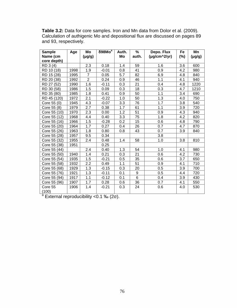
76

Table 3.2: Data for core samples. Iron and Mn data from Dolor et al. (2009). Calculation of authigenic Mo and depositional flux are discussed on pages 89 and 93, respectively.

Sample Name (cm core depth)

Age Mo (µg/g)

δ98Moa Auth. Mo

% auth.

Depo. Flux (µg/cm^2/yr)

Fe (%)

Mn (µg/g)

RD 3 (4) 2.3 0.18 1.4 59 1.6 3.6 600 RD 10 (18) 1998 1.9 -0.01 0.8 41 0.9 4.2 980 RD 15 (28) 1995 7 0.05 5.7 82 6.9 4.8 840 RD 20 (38) 1992 2 0.24 0.9 46 1.1 4.1 940 RD 27 (52) 1990 1.6 -0.11 0.3 21 0.4 4.8 1220 RD 30 (58) 1986 1.5 0.09 0.3 18 0.3 4.7 1210 RD 35 (80) 1985 1.8 0.41 0.9 50 1.1 3.4 690 RD 45 (120) 1972 2.1 -0.22 1.0 50 1.3 4.0 750 Core 55 (0) 1945 4.3 -0.07 3.3 76 1.7 3.8 540 Core 55 (8) 1979 2.7 0.38 1.7 61 1.1 3.9 720 Core 55 (10) 1970 2.3 0.00 1.2 51 0.9 4.3 940 Core 55 (12) 1968 4.4 0.40 3.3 75 1.8 4.2 820 Core 55 (16) 1966 1.5 -0.28 0.2 15 0.6 4.8 790 Core 55 (20) 1964 1.7 0.27 0.4 26 0.7 4.7 870 Core 55 (26) 1963 1.8 0.80 0.8 43 0.7 3.9 840 Core 55 (28) 1957 9.5 0.34 3.8 Core 55 (32) 1955 2.4 0.48 1.4 58 1.0 3.8 810 Core 55 (38) 1951 0.25 Core 55 (44) 2.4 0.40 1.3 54 1.0 4.1 980 Core 55 (50) 1940 1.4 0.21 0.3 21 0.6 4.2 730 Core 55 (54) 1935 1.5 -0.21 0.5 35 0.6 3.7 650 Core 55 (58) 1932 2.2 0.49 1.1 51 0.9 4.1 710 Core 55 (68) 1929 1.3 -0.15 0.3 20 0.5 3.9 700 Core 55 (76) 1921 1.3 -0.11 0.1 9 0.5 4.4 720 Core 55 (94) 1917 1.1 -0.12 0.1 6 0.4 3.9 430 Core 55 (96) 1907 1.7 0.28 0.6 36 0.7 4.1 550 Core 55 (100)

1906 1.4 -0.21 0.3 24 0.6 4.0 530

a External reproducibility <0.1 ‰ (2σ).

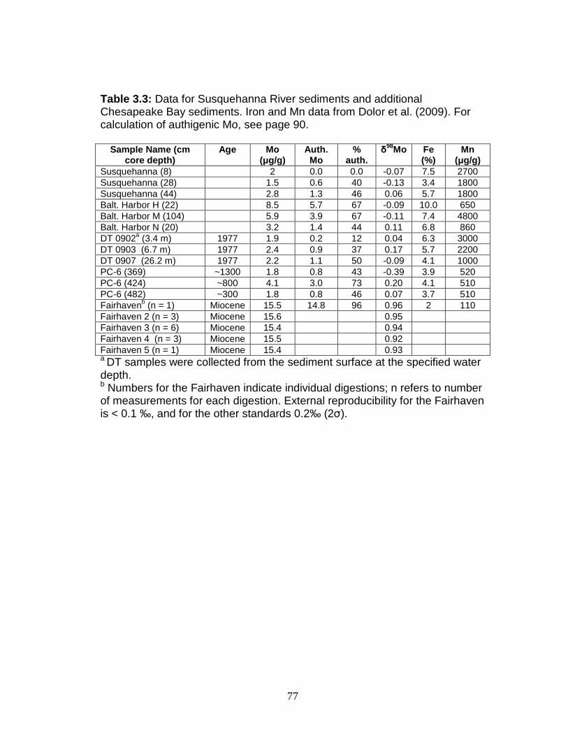
77

Table 3.3: Data for Susquehanna River sediments and additional Chesapeake Bay sediments. Iron and Mn data from Dolor et al. (2009). For calculation of authigenic Mo, see page 90.

Sample Name (cm core depth)

Age Mo (µg/g)

Auth. Mo

% auth.

δ98Mo Fe

(%) Mn

(µg/g) Susquehanna (8) 2 0.0 0.0 -0.07 7.5 2700 Susquehanna (28) 1.5 0.6 40 -0.13 3.4 1800 Susquehanna (44) 2.8 1.3 46 0.06 5.7 1800 Balt. Harbor H (22) 8.5 5.7 67 -0.09 10.0 650 Balt. Harbor M (104) 5.9 3.9 67 -0.11 7.4 4800 Balt. Harbor N (20) 3.2 1.4 44 0.11 6.8 860 DT 0902a (3.4 m) 1977 1.9 0.2 12 0.04 6.3 3000 DT 0903 (6.7 m) 1977 2.4 0.9 37 0.17 5.7 2200 DT 0907 (26.2 m) 1977 2.2 1.1 50 -0.09 4.1 1000 PC-6 (369) ~1300 1.8 0.8 43 -0.39 3.9 520 PC-6 (424) ~800 4.1 3.0 73 0.20 4.1 510 PC-6 (482) ~300 1.8 0.8 46 0.07 3.7 510 Fairhavenb (n = 1) Miocene 15.5 14.8 96 0.96 2 110 Fairhaven 2 (n = 3) Miocene 15.6 0.95 Fairhaven 3 (n = 6) Miocene 15.4 0.94 Fairhaven 4 (n = 3) Miocene 15.5 0.92 Fairhaven 5 (n = 1) Miocene 15.4 0.93 a DT samples were collected from the sediment surface at the specified water depth. b Numbers for the Fairhaven indicate individual digestions; n refers to number of measurements for each digestion. External reproducibility for the Fairhaven is < 0.1 ‰, and for the other standards 0.2‰ (2σ).

78

Methods

Sample preparation and measurement

Complete details for all methods are provided Chapter 2, but a brief

overview is provided here. Finely powdered sediments (0.2 to 0.5 g) and

acidified water samples (1 to 5 L) were spiked with a 97Mo-100Mo double spike

solution (29.39 µg/g Mo in 2% nitric acid), to correct for analytical mass bias

(e.g., Siebert et al., 2001). Sediment samples were then digested with

concentrated, high-purity acids. Trace metals from water samples were pre-

concentrated using a chelating resin, according to the method of T. Dahl

(personal communication). Chromatographic separation, using anion and

cation exchange resins, was used to purify Mo from all samples (Pietruszka et

al., 2006). Blanks for the 3-column chemistry ranged between 2 and 6 ng Mo,

comprising less than 1% of the total Mo for all sediment samples. The blank

for processing one liter of distilled water was 0.22 µg, or approximately 4% of

the water-sample Mo for the estuarine samples. This quantity of blank

contributes ~20% of the Mo to the Susquehanna River sample, because of its

lower Mo concentration, leading to the possibility that the isotopic ratio for this

sample is slightly biased.

Measurements were made using a Nu Instruments multi-collector ICP-

MS at the University of Maryland. Raw isotope ratios were reduced using a

modified version of the iterative scheme introduced by Siebert et al. (2001).

Delta values were calculated using the standard notation: δ98Mo = ((98/95Mo

sample/ 98/95Mo standard)-1)*1000, where the standard is an in-house

Johnson-Matthey Company SpecPure® Mo plasma standard (Lot # 013186S),

79

and its 98/95Mo ratio is fractionation-corrected by measuring double-spiked

aliquots and reducing the raw data.

Maximum long-term external reproducibility of two in-house rock

reference standards is ±0.20‰ for δ98Mo at the 2σ level (Chapter 2). Five

separate digestions of the Fairhaven sample, and multiple analyses of each

processed digestion, have a 2σ of ±0.09‰. Concentration data derived from

the double-spike data for the Fairhaven have approximate uncertainties of

±1% (15.5 ±0.1 µg/g), which likely includes some sample heterogeneity.

In order to facilitate comparison with published results from other

institutions, a widely available seawater standard (CASS-4, National

Research Council Canada) was processed and analyzed. The sample had a

Mo concentration of 8.84 µg/L, compared to the certificate value of 8.78 ±

0.86 µg/L. This concentration is ~10% lower than that of open-ocean

seawater (e.g., Collier, 1985), possibly because the CASS-4 water was

collected in a harbor, and has a salinity of 30.7. The Mo isotopic value was

+2.23 ± 0.09‰ (2σ), within the analytical uncertainty for one published

measurement of seawater (+2.3 ± 0.1‰; Siebert et al., 2003), but outside

the uncertainty of another measurement (+2.45 ± 0.11‰; Nakagawa et al.,

2008). The lower δ98Mo, compared to previous results, could be a result of

either the lower salinity or lower Mo concentration relative to open-ocean

seawater, or a consequence of normalizing to different batches of SpecPure®

Mo used by the other researchers.

80

Calculation of authigenic Mo

Conventionally, Mo in bulk sediment digestates is regarded as

consisting of lithogenic Mo and authigenic Mo, the latter being ultimately

derived from dissolved Mo in the water column. A quantity termed Moauth can

be calculated in order to characterize the authigenic component of Mo

present in a sample (e.g., Adelson et al., 2001). This calculation

mathematically removes the lithogenic Mo component from a sample by

normalizing to an element whose concentration is largely lithogenic in nature.

In this study, normalization is done with Fe for analytical reasons (Dolor et al.,

2009), rather than the commonly preferred, diagenetically immobile Al. As

shown by the extensive study of Daskalakis and O'Connor (1995), either

element may be used in estuarine and near-shore waters, because deposition

rates of Fe are much faster than the diagenetic mobility of Fe. Thus, its

vertical distribution is not measurably affected by diagenesis.

Normalizing removes concentration variations that are due to changes

in grain size within cores, and allows different sediment types from disparate

localities within the Bay, such as the Susquehanna River (mostly sand) and

PC-6 (homogenous clay), to be compared. The operational definition

(Adelson et al., 2001) for Moauth is:

(3.1) Moauth = Momeas - [Femeas * (Mo/Fe)lith]

In this formulation, the lowest Mo/Fe ratio in the sample set is used to define

the (Mo/Fe)lith, because such a sample would imply the greatest crustal

81

content, and be representative of the local background with respect to Mo.

The Susquehanna River sample from 8 cm satisfies this definition (2.7 x10-5);

the oldest sample from Core 55 (96 cm, ~1900) also has a similarly low

Mo/Fe ratio (2.8 x10-5).

Results

Chesapeake Bay and Susquehanna River water

Dissolved Mo concentrations for six mid-depth and two near-bottom water

samples show a non-linear distribution with salinity, indicating a small degree

of Mo removal from the water column within the estuary (Fig. 3.2a). Non-

conservative behavior of Mo has previously been reported by van den Berg

(1993), who also proposes removal within mesohaline regions (salinity of 7-20

psu) to explain the contrast to conservative behavior of Mo in the ocean. The

Mo concentration versus salinity distribution is similar to that found by

Kingston et al. (1983). Bottom samples fall on the same concentration versus

salinity curve as mid-depth samples (Fig. 3.2a).

Susquehanna River water has a measured Mo concentration of 0.27

µg/L (Table 3.1). This is roughly one-half of the amount estimated or

measured for rivers globally (e.g., Archer and Vance, 2008; Martin and

Maybeck, 1979). The regression of Mo concentration in the Bay vs. salinity

(Fig. 3.2a) extrapolates to a similar, but slightly lower, Mo concentration for

the river (0.2 µg/L). Susquehanna River water has a relatively long residence

time after it enters the northern, oligohaline Bay (~6 months). Therefore, the

82

extrapolated value may be a better estimate of the time-averaged Mo

concentration in water derived from the Susquehanna River.

The measured δ98Mo of the river water, +1.02‰ (± 0.09, 2σ), is within

the range of values measured in other rivers by Archer and Vance (2008).

The isotopic composition of dissolved Mo in the Bay (Fig. 3.2b) appears to be

dominated by seawater. This can easily be attributed to the much higher

concentration of Mo in seawater than in river water. For the six samples with

salinity >15 psu, where little Mo is being contributed by river water, the

average δ98Mo is +2.17 ± 0.12, in good agreement with values for seawater.

In the vicinity of cores 55 and RD, the seasonal range of salinity is 5 to 15

psu, and δ98Mo in this water is not greatly different from that in seawater. This

establishes that dissolved Mo in Chesapeake Bay, the source of authigenic

Mo at these sites, is isotopically heavy.

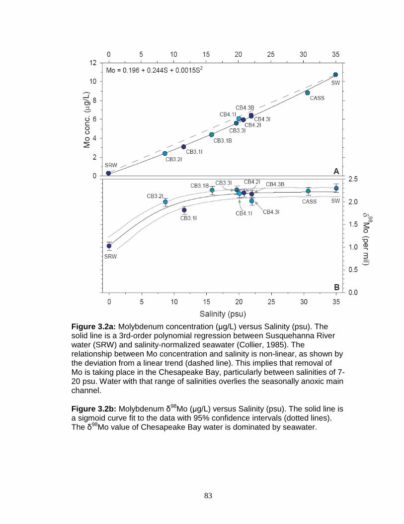
83

Figure 3.2a: Molybdenum concentration (µg/L) versus Salinity (psu). The solid line is a 3rd-order polynomial regression between Susquehanna River water (SRW) and salinity-normalized seawater (Collier, 1985). The relationship between Mo concentration and salinity is non-linear, as shown by the deviation from a linear trend (dashed line). This implies that removal of Mo is taking place in the Chesapeake Bay, particularly between salinities of 7-20 psu. Water with that range of salinities overlies the seasonally anoxic main channel.

Figure 3.2b: Molybdenum δ98Mo (µg/L) versus Salinity (psu). The solid line is a sigmoid curve fit to the data with 95% confidence intervals (dotted lines). The δ98Mo value of Chesapeake Bay water is dominated by seawater.

84

Chesapeake Bay and Susquehanna River sediments

Molybdenum concentrations for cores RD and 55 are presented in

Figure 3.3a and Table 3.2. In Figure 3.3b, the depositional flux of Moauth is

presented. To obtain these values, the calculated Moauth (Eq. 3.1) is multiplied

by the appropriate sediment mass accumulation rate (Fig. 3.3b, Table 3.2). In

the first two decades of the 20th century, very little Moauth accumulated in the

deep channel of Chesapeake Bay, similar to the results of Adelson et al.

(2001). Subsequently, Moauth fluxes increased, although inter-annual

variability remained high throughout the century.

Molybdenum isotopic data for cores RD and 55, versus deposition

date, are presented in Figure 3.4. In samples from the first two decades of the

century, four of the five δ98Mo values are < 0‰. Subsequently, the number of

positive δ98Mo values increases. The 3-fold higher deposition rate in core RD,

compared to core 55, implies that the RD site receives significantly more

sediment input, which seems to dilute the impact of Moauth formation on the

Mo isotopic composition of the bulk sediment. The Susquehanna River

sediments (Table 3.3) have low Mo concentrations, and an average δ98Mo

value of -0.05‰ (± 0.09) (Fig. 3.5). Similarly, surface samples from the depth

traverse (DT) also have low Mo concentrations, with no trend related to water

depth or Mn concentration (Table 3.3). The average δ98Mo value for the three

DT samples is +0.04‰ (± 0.13), not analytically distinct from the

Susquehanna River sediment samples. Based on these samples, the Mo

isotopic composition of the lithogenic material delivered to the Bay by the

85

Figure 3.3a: Molybdenum concentration (µg/g) versus age/depth for cores RD and 55. On the y-axis, depth has been translated to date of deposition (age) using the deposition rates given by Helz et al. (1985a) and Zimmerman and Canuel (2002).

Figure 3.3b: Depositional flux of authigenic Mo versus age/depth for cores RD and 55. Note a break in scale between 2 and 6 µg/cm2/yr. For discussion of depositional flux, see page 93.

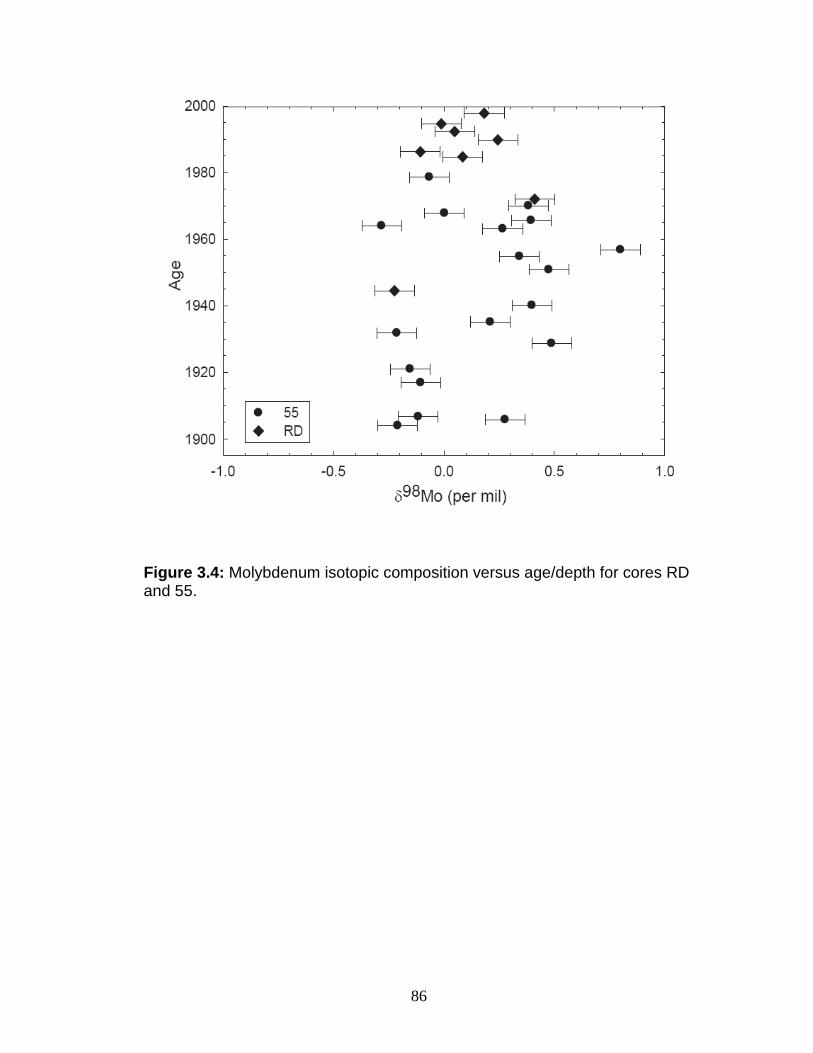
86

Figure 3.4: Molybdenum isotopic composition versus age/depth for cores RD and 55.

87

Susquehanna River appears to be indistinguishable from the presumed global

continental crust value of ~0‰ (Siebert et al., 2003).

Baltimore Harbor sediments differ from the preceding samples in

having higher Mo concentrations, from 3.2 to 8.5 µg/g (Fig. 3.5), but are

similar in Mo isotopic composition (Table 3.3). The elevated Mo

concentrations could be anthropogenic, or a result of microbial sulfate

reduction. The isotopic similarity of these contaminated sediments to

uncontaminated sediments elsewhere in the Bay suggests that anthropogenic

Mo contamination does not impose a distinctive isotopic signature that could

be used as a contaminant tracer (in contrast with 187Os/188Os; Helz et al.,

2000).

The three samples from core PC-6 predate the arrival of European

agriculture (1675-1775), and therefore provide insight to historical Mo

behavior in the Bay. In this context, they can be compared with the early 20th

century, pre-eutrophication core samples. Two of the three PC-6 samples

have Mo concentrations averaging 1.8 µg/g, while one sample (~800 ybp) has

a higher concentration of 4 µg/g. The topmost sample (~1300 ybp) is

isotopically light (-0.39‰), possibly a reflection of greater MnOx formation.

The other two samples are not resolvable from 0‰, the presumed signature

of lithogenic Mo derived from the Susquehanna Basin. The Mo in the PC-6

samples is similar in concentration and isotopic composition to the Mo in

Susquehanna River sediments. This could be an indication that most of the

88

Mo in these samples was derived from bed load, as opposed to authigenic

processing of Mo derived from the water column.

A Mo-rich (15 µg/g) sediment sample from the Miocene Fairhaven cliffs

has the highest Mo concentration and heaviest Mo isotopic composition

(+0.97‰) measured for the entire Chesapeake Bay suite. The isotopic

composition and relative enrichment in Mo of this formation suggest it may

have been deposited in a suboxic basin or lagoon. Shoreline erosion of the

Mo-rich Fairhaven outcrop has been hypothesized as a source of Mo

enrichment in PC-6 sediments (Adelson et al., 2001), but the outcrop lies too

far to the south for it to be a likely sediment source at the Core 55 and RD

sites.

Discussion

Authigenic Mo formation in the Chesapeake Bay

In the absence of anoxic conditions, it might be expected that the Mo

concentration and δ98Mo values of Bay sediments would be similar to the

concentration and δ98Mo values of Susquehanna River sediments, based on

the simple paradigm that Mo in river-transported detrital bed load is deposited

within the Bay, while Mo dissolved in river water and seawater transits the

estuary unaltered. In the modern day, the dissolved Mo distribution in the

waters of Chesapeake Bay is not conservative (Fig. 3.2a), implying that Moauth

is forming in the Bay. Additionally, core samples deposited after 1925 have

higher Mo concentrations and more Moauth, compared with samples deposited

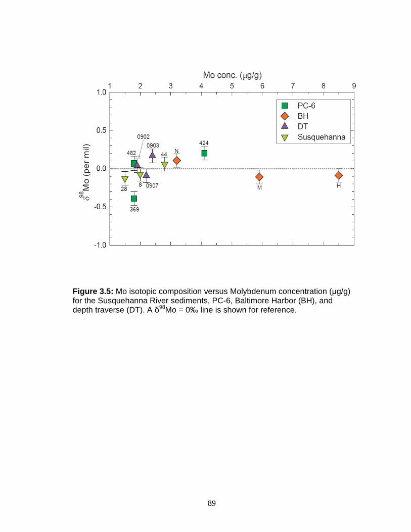
89

Figure 3.5: Mo isotopic composition versus Molybdenum concentration (µg/g) for the Susquehanna River sediments, PC-6, Baltimore Harbor (BH), and depth traverse (DT). A δ98Mo = 0‰ line is shown for reference.

90

before 1925 (Figures 3.3a and 3.3b). The implication is that a persistent

change in deep water sedimentation took place sometime after 1925. This

change likely involved an increase in intensity and occurrence of seasonal

anoxia (Cooper and Brush, 1993, Adelson et al., 2001). In 1960, a period of

decreased Moauth is likely the result of low river flow during a prolonged

drought. Recent monitoring of the Bay has shown that low river flow tends to

reduce the extent and severity of coastal eutrophication (Hagy et al., 2004).

The considerable scatter in the Mo concentrations of the core samples

after 1925 might be due to the great variation in the extent of seasonal anoxia

from year to year, heavily influenced by spring runoff and nitrate loading

(Hagy et al., 2004). For example, between the summers of 1985 and 1986,

the volume of moderately hypoxic water (dissolved O2 < 2 mg/L) changed

from 4.4 x 109 m3 to 11.0 x 109 m3, but between 1959 and 1960 only changed

from 4.9x109 m3 to 4.2x109 m3 (Hagy et al., 2004). Therefore, we conclude

that the Moauth profile for cores RD and 55 most likely reflects super-annual

variations in anoxia.

The core RD and 55 data display a wide range of both isotopic values

and amounts of Moauth (Fig. 3.6). Although there is a general trend relating

heavier δ98Mo values with more Moauth, the scatter is large, and R2 is low

(+0.18). This indicates that the processes controlling Moauth and δ98Mo are

substantially independent of one another (Fig. 3.6). The regression line

indicates that a lithogenic end member (Moauth = 0%) should have δ98Mo =

-0.11‰, while the authigenic end member has δ98Mo = +0.45‰. The upper

91

and lower dotted lines represent mixing of lithogenic Mo with seawater Mo

and MnOx-derived Mo, respectively. Within error, these lines enclose all the

data for cores RD and 55, suggesting that the samples can be derived by

mixing Moauth from MnOx with dissolved Mo from seawater, plus lithogenic

Mo. The regression line (Fig. 3.6) suggests that the most common Mo

isotopic composition of the Moauth mixing end- member is approximately

+0.45‰, implying that Moauth in a typical year is derived 60% from MnOx and

40% from seawater Mo. However, the scatter of the data implies that the

proportions of Moauth derived from MnOx and seawater vary greatly from year

to year. It is important to note that sediment deposition rates in Chesapeake

Bay are on the order of 103 times faster than typical deep-sea rates. The

implication for Moauth is that, in order to avoid dilution of the signal, the

process delivering Moauth to the sediments must be very robust indeed.

In many settings, organic carbon is the most important carrier of Mo, and

sediments often show a high degree of correlation between organic carbon

contents and Mo (Tribovillard et al., 2004). However, when the organic matter

has not been sulfurized and the S is in the pyrite form, this correlation

disappears (Tribovillard et al., 2004). In Chesapeake Bay, low organic carbon

contents (1.8 to 3.3%) show no relationship to amount of Moauth, similar to the

latter example (Appendix 1). This suggests that, in this estuary, organic

carbon plays a more limited role in influencing Moauth than in other

environments.

92

Figure 3.6: Percent of authigenic Mo versus Mo isotopic composition for the data of cores RD and 55 (all grey squares, not differentiated by core). Solid lines are a linear regression through the data with 95% confidence intervals. Upper dotted line represents a mixing line for lithogenic Mo with seawater, lower dotted line represents a mixing line for MnOx-derived Mo with lithogenic Mo. The regression equation yields an estimate for the isotopic composition of continental material contributed by the Susquehanna Basin (-0.11‰), and an upper value for a hypothetical sample with 100% authigenic Mo of approximately +0.45‰.

93

Molybdenum isotope fractionation in Chesapeake Bay sediments

Molybdenum in sediments from the main channel of Chesapeake Bay

is, in most cases, isotopically heavier than lithogenic Mo, but lighter than

dissolved Mo (as MoO42-) in the overlying water (Fig. 3.6). A feasible

mechanism must explain both the variability in isotopic composition and the

range of Moauth content. Many processes that result in Mo isotopic

fractionation have been identified, for example, microbial metabolism

(Wasylenki et al., 2007), carbonate deposition (Voegelin et al., 2009), and Fe

oxide precipitation (Malinovsky et al., 2007; Goldberg et al., 2009). Two

processes result in fractionations that are both large and distinct, MnOx

precipitation and thiomolybdate formation. Many of the other recently

identified fractionation mechanisms result in isotope values within the

brackets established by MnOx and thiomolybdate (Fig. 3.6), and therefore

may not be easily distinguishable from one another in a complex system.

When H2S reacts with MoO42-, thiomolybdates are formed. If

theoretical calculations are correct (Tossell 2005), thiomolybdate should be

isotopically light relative to the starting MoO42-. If H2Saq exceeds ~11 µM, the

conversion can become quantitative, given sufficient time for the reaction to

take place (Erickson and Helz, 2000). In this case, no fractionation will be

detected, as the thiomolybdate product will have the same isotopic

composition as the starting MoO42-. Where H2Saq values are below the switch-

point, selective scavenging of thiomolybdate, from a mixture of MoO42- and

thiomolybdate, might occur. Such a process has been proposed to explain the

94

isotopic composition of surface sediments from varying water depths in the

Black Sea (Neubert et al., 2008).

Invoking fractionation associated with thiomolybdate formation to form

authigenic Mo that is lighter than the MoO42- in the water column is

problematic for Chesapeake Bay. In contrast to the Black Sea (e.g., Neubert

et al., 2008), a thiomolybdate-based mechanism probably never operates in

the Chesapeake Bay water column because the requisite H2Saq levels rarely

obtain (Lewis et al., 2007). One model for Moauth formation in estuaries

proposes that MoO42- diffuses from the water column into the pore water,

where it eventually reaches the H2Saq = 11 µM isopleth (Adelson et al., 2001;

Boothman and Coiro, 2009). At that horizon, thiomolybdate formation is

activated. In this model, seasonal fluctuation of the 11 µM isopleth depth

within the sediments exerts control on the rate of Moauth formation. Although

Mo geochemistry in pore water is not well understood, several studies

suggest that Mo is nearly quantitatively removed from pore water at this

horizon (Colodner et al., 1993; Morford et al., 2007; Zheng et al., 2000).

However, quantitative removal from pore water would produce Moauth with

δ98Mo values identical to the overlying water. This appears to be inconsistent

with Figure 3.6.

Alternatively, delivery of isotopically light Mo to the pore waters can be

easily accomplished by dissolution of MnOx particles. During episodes of

water column anoxia in Chesapeake Bay, Mn refluxing takes place (Eaton,

1979; Helz et al., 1985b). Refluxing involves reduction of surface-sediment

95

MnOx to Mn2+, which can be transported upwards through the anoxic zone,

until it encounters oxic near-surface waters. In this zone, MnOx particles can

re-form, fractionating Mo during adsorption (e.g., Wasylenki et al., 2008). The

MnOx particles eventually sink back to the sediment surface, carrying Mo that

is isotopically lighter than that in the overlying water. This Mo is released as

the Mn cycle is repeated. At sites near Core RD, Shaw et al. (1994) show that

dissolved Mn2+ rises 1000-fold in bottom waters during spring, reaching

summertime peaks of several µM after O2 disappears. Eaton (1979) found

that in summer, Mn is solubilized from surface sediments fast enough to

replace the dissolved Mn concentration in 20 m of bottom water in less than

two weeks. Furthermore, Moffett (1994) showed that Mn2+ diffusing into oxic

surface water is oxidized to particulate MnOx at rates exceeding 2000% per

day. These findings imply that Mn can be recycled many times during the

summer months, and each cycle has the potential to release isotopically light

Mo into the water near the sediment-water interface. Once isotopically light

Mo builds up, it can be subsequently fixed as Moauth after diffusing to the

11µM H2Saq horizon. This is similar to the scheme proposed by Reitz et al.

(2007).

A key difference between the thiomolybdate and MnOx mechanisms is

the location in which the fractionation from isotopically heavy dissolved Mo to

isotopically light Mo occurs. In the first mechanism, fractionation occurs near

the 11µM H2S horizon in the sediments (e.g., Neubert et al., 2008). This

would result in an isotopically heavy MoO42- 'residue' in the pore water, but it

96

is not obvious how this residue could be selectively returned to the water

column. In the second mechanism, fractionation occurs in the water column,

removed from the site of Moauth formation.

The MnOx mechanism is attractive because the processes that control

Moauth formation (pore water H2Saq) and δ98Mo (MnOx) are separate, even

though both are influenced by seasonal oxygen stress in the estuary. This is

consistent with the positive relationship, but low correlation coefficient,

between δ98Mo values and percentage of Moauth in the core data (Fig. 3.6).

Isotopic mass balance in the Chesapeake Bay watershed

The average sediment discharge from the Susquehanna Basin to the

Bay is 5 x 1012 g/y (Gross et al., 1978). The composition of this sediment is

estimated at 1.4 x 10-6 g Mo/g sed, giving a Mo flux from the watershed of 7.0

x 106 g Mo/y as solid material. Freshwater discharge averages 34.7 x 109

m3/y or 3.47 x 1016 g H2O/y (Schubel and Pritchard, 1987). Based on the Mo

concentration of the Susquehanna River, the dissolved Mo in river water is

about 0.2 x 10-9 g Mo/g H2O, making the mass of dissolved Mo leaving the

basin about 6.9 x 106 g Mo/y. The mass of Mo leaving the Susquehanna

basin in solid versus dissolved form appears to be roughly equal, in

agreement with findings for the world's large rivers (Martin and Meybeck,

1979).

This simple Mo budget indicates that an isotopic mass balance

problem might exist for the Susquehanna watershed. Pre-1925 sediment

samples from Core 55, as well as sediments from the Susquehanna River

97

itself, suggest that δ98Mo in sediments from the watershed is about -0.1‰. In

contrast, δ98Mo in the water is +1.02‰. Although this latter value is based on

only one measurement, it is consistent with the broader findings of Archer and

Vance (2008). Assuming those isotopic values are typical of solid-phase and

dissolved Mo, then either the average δ98Mo of rocks that are undergoing

weathering in the basin is closer to +0.5‰, as opposed to the generally

assumed 0‰, or weathering and erosion in the basin are not in steady state.

Release of water with δ98Mo = +1.02‰ from a basin averaging 0‰ would

require that either a reservoir of isotopically light solid material is forming

somewhere in the basin, or that isotopically heavy rocks are presently being

selectively weathered. A plausible hypothesis based on the latter possibility

posits that black shale associated with extensive coal deposits in the basin is

being leached at an accelerated rate by acid mine drainage. Investigation of

Mo isotopes in the Susquehanna River basin is a topic for future study.

Conclusions

The Chesapeake Bay sediments display a range of δ98Mo that is

~1.2‰. All samples are offset from the water-column isotopic composition by

at least ~1‰. The δ98Mo range is somewhat smaller than that of the suboxic

regimes described by Siebert et al. (2006), and is much larger than would be

expected of a pure anoxic system (Poulson et al., 2006). In common with

previous research, Mn-rich sediments in Chesapeake Bay contribute

isotopically light Mo, but this signature is diluted by mixing with other

components and low total amounts of Moauth.

98

There is significant evidence that fractionation of Mo isotopes is

occurring during sedimentation in the Chesapeake Bay, and that the isotopic

composition of these sediments is distinctly different from the composition of

major Mo sources to the Bay. We propose a mechanism that provides a

satisfactory explanation for the observed trends in the Mo isotope data and

Moauth concentrations from core samples in the seasonally anoxic main stem

of the Bay. Sediment samples from the past century show a distinct change in

sedimentation since 1925, as inferred from Mo isotope values, indicating an

increase in the severity of coastal eutrophication, and increased efficiency of

the Moauth formation mechanism.

99

Chapter 4: Molybdenum isotopic signatures in Pliocene-Pleistocene aged Mediterranean sapropels 3

Abstract In the sediments of the Mediterranean Basin, unusual organic carbon-

rich layers, known as sapropels, occur at regular intervals that correspond to

orbital insolation cycles. These layers are enriched in trace metals that are

sensitive to low-O2 conditions, such as Re and Mo. Sapropel deposition is,

most likely, the result of a highly specific set of conditions that include

hydrographic changes that encourage development of anoxic conditions.

Molybdenum isotopes have the potential to discriminate between a variety of

scenarios for sapropel deposition, such as localized or basin-wide anoxia,

'suboxic' conditions, or euxinia.

The Mediterranean evidently switched rapidly and often from an oxic

state to an anoxic state. δ98Mo values for sapropels and spatially associated

hemipelagic sediments vary greatly, ranging from -0.6 to +3.5‰. The heaviest

isotopic values are primarily found in the hemipelagic sediments and rarely

within the sapropel layers. However, it might be expected that if anoxic

conditions prevailed during sapropel deposition, a seawater isotopic

composition (~+2.3‰) would be evident in the layer. Comparison between Mo

isotopic compositions of sapropel layers and compositions present in normal

marine sediments suggest that low-O2 conditions sometimes prevailed during

the 'normal' segment of the depositional cycle, and are responsible for heavy

3 This research used samples and/or data provided by the Ocean Drilling Program (ODP).

ODP is sponsored by the U.S. National Science Foundation (NSF) and participating countries under management of Joint Oceanographic Institutions (JOI), Inc.

100

isotopic compositions during those times. Given the very high amounts of

organic carbon present, it also may be possible that sinking organic matter

was an important carrier of Mo in this environment.

Introduction Beginning in the earliest Pliocene, and continuing into the Holocene,

the Mediterranean Basin saw the onset of deposition of sapropels, which are

cyclic, laminated, organic-rich (>2% TOC) sedimentary layers (Sakamoto et

al., 1998). Numerous studies using a variety of lines of evidence have

concluded that sapropel deposition occurred as a result of anoxic conditions

that prevailed in the Mediterranean Sea during this period (e.g., Rossignol-

Strick et al., 1982; Passier et al., 1999; Emeis et al., 2000; Larrasoana et al.,

2003; Scrivner et al., 2004). Anoxic conditions, coupled with high primary

productivity, appear responsible for many of the unique features observed in

the sapropel layers, including high organic carbon contents (e.g., Cramp and

O’Sullivan, 1999; Sancetta, 1999), and enrichments in elements that are

redox sensitive, such as V, Mo, and Re, relative to both continental crust and

average shale (Nijenhuis et al., 1998; Warning and Brumsack, 2000;

Wehausen and Brumsack, 1998).

There is considerable evidence that the anoxic conditions were

instigated by vast inputs of fresh water that diluted the normally hypersaline

(38 psu) Mediterranean Sea surface waters (Thunell and Williams, 1989;

Kroon et al., 1998). A freshening event would likely prevent sinking of surface

water, which currently keeps the bottom waters of the Eastern Mediterranean

101

aerated to the level of about 60% of the air saturation value appropriate for

their temperature and salinity. Freshening, therefore, would weaken

formation of new, oxygen-rich deep water masses (Rossignol-Strick et al.,

1982), and weaken the normal anti-estuarine circulation pattern. In this

situation, deep water ventilation would be low, and result in suboxic

conditions (Stratford et al., 2000). Alternatively, it has been suggested that,

with a fresh water cap, the circulation would reverse to an estuarine type, and

intermediate water would enter from the Western Mediterranean basin over

the 300 m deep sill at the Strait of Sicily (Stratford et al., 2000). In this mode,

deep waters would become anoxic. Under any set of conditions in which deep

waters are not being quickly renewed, oxygen utilization will quickly outstrip

the supply in the deep waters (Rohling, 1994), resulting in suboxic or anoxic

conditions. Sapropels could, therefore, form under either weak anti-estuarine

or estuarine circulation, but those formed under the estuarine circulation

(anoxic mode) would be the most organic-carbon rich (Stratford et al., 2000).

The delivery of fresh water needed to repeatedly limit deep-water

ventilation has been linked to the direct influence of high-latitude insolation

maxima, through eccentricity-modulated precessional minima (e.g., Hilgen,

1991). Eccentricity minima influence low-latitude (African) monsoon cycles,

and the Mediterranean is affected by increased Nile River flow (Rossignol-

Strick, 1983; Tuenter et al., 2003).

Despite this conceptual understanding, many issues remain

unresolved regarding sapropel deposition in the Mediterranean, especially

102

considering that conditions likely varied for individual sapropels. For example,

although the effects of diagenesis during basin re-oxygenation have been

studied (Jung et al., 1997; Thomson et al., 1995), many aspects of this

process remain poorly understood. Also, the high trace metal contents in the

sapropels require a renewable source. While this source is likely to be

seawater (e.g., Nijenhuis et al., 1998), mechanisms and rates of replacement,

as well as possible changes in the amount of exchange between the Eastern

and Western Mediterranean during anoxic episodes remain little explored.

The thickness of the oxygen-deprived deep layer is also debated (e.g.,

Casford et al., 2003).

Redox-sensitive trace elements, such as Fe, V, Mo, and Re, in oceanic

sediments/sedimentary rocks have commonly been used as proxies for

paleoredox and paleoproductivity (e.g., Bertine and Turekian, 1973, Emerson

and Huested, 1991; Calvert and Pedersen, 1993; Colodner et al., 1993;

Crusius et al., 1996; Zheng et al., 2000; Wilde et al., 2004; Tribovillard et al.,

2004, 2006, Morford et al., 2005, 2009; Algeo and Lyons, 2006). The

dramatic changes in solubility of these elements under different degrees of

oxygen depletion may be reflected in their relative and absolute

concentrations recorded in sediments (Tribovillard et al., 2006). Molybdenum

isotopes can also be used to provide complementary information regarding

paleoredox conditions (e.g., Reitz et al., 2007; Neubert et al., 2008; Pearce et

al., 2008; Gordon et al., 2009; Poulson-Brucker et al., 2009). Dissolved

MoO42- is relatively inert, while MoS4

2-, which forms under sulfidic conditions,

103

is readily scavenged by sinking particles (Vorlicek et al., 2004). This

dichotomous behavior, coupled with isotopic fractionation resulting from

adsorption to sedimentary particles, sets the framework for the utility of Mo

isotopes. Seawater has been shown to have a relatively uniform δ98Mo of

+2.3‰ (e.g., Siebert et al., 2003; Nakagawa et al., 2008), so sediments

deposited in fully euxinic conditions (H2Saq > 11 µM; Erickson and Helz, 2000)

tend to record the δ98Mo of seawater as a result of quantitative Mo removal

(e.g., Neubert et al., 2008). Conversely, sediments that form in oxic seawater

are more likely to have δ98Mo lighter than seawater as a result of processes

such as Mn-oxide formation, which preferentially adsorbs light Mo isotopes

(Barling and Anbar, 2004; Wasylenki et al., 2008).

Here, we examine absolute and relative abundances of V, Mo, Re, in

conjunction with Mo isotopes, to discern amongst the complex depositional

signals that are likely recorded in Mediterranean sapropels. These include

climatic signals, water column processes, and possible diagenetic

overprinting. We address, primarily, the question of the state of the water

column during sapropel deposition, and the conditions that obtained during

hemipelagic sedimentation. We discuss how this type of dynamic system

differs fundamentally from the type locality for euxinic deposition (the Black

Sea), and from oxic, 'suboxic' and anoxic regimes. However, some similarities

with all these depositional types will be identified and discussed.

104

Background

Mediterranean hydrography

The Mediterranean Sea consists of the Eastern Mediterranean and

Western Mediterranean, two large basins that are separated by an ~330 m

deep sill in the Strait of Sicily, and from the Atlantic Ocean by the 280 m sill in

the Strait of Gibraltar. Circulation is characterized by relatively free eastward

exchange of surface water, including inflow from the Atlantic Ocean, and

westward exchange of subsurface water (Rohling, 1994). This anti-estuarine

flow pattern is driven by the excess of evaporation over precipitation

(Bethoux, 1980). Evaporation and warming takes place in the surface water

as it flows eastward, altering the density and salinity parameters (Millot and

Taupier-Letage, 2005). This warm, very salty water sinks during localized

convective cooling episodes, and oxygen-rich intermediate and deep water

masses are formed (Millot and Taupier-Letage, 2005). The main mass of

Mediterranean intermediate water forms in the Levantine basin, and Eastern

Mediterranean deep water forms in the Adriatic Sea as a result of intense

winter cooling (Robinson et al., 2001; Rohling 1994). Deep convective mixing,

which presently keeps the deep parts of both basins well oxygenated, is

encouraged by net buoyancy loss (Rohling 1994). Complete renewal of the

deep water below 1500 m is estimated to take between 80 (Schlitzer et al.,

1991) and 150 years (Roether and Well, 2001). During sapropel deposition,

influx of fresh water to the surface layer likely prevented normal convective

mixing, weakened the circulation pattern, and possibly led to stratification of

the water column, on the scale of ~1000 years (e.g., Rossignol-Strick et al.,

105

1982). The set-up of the estuarine circulation pattern, where the Western

Mediterranean supplies a limited quantity of deep water beneath the buoyant

surface layer, has also been suggested (Stratford et al., 2000; Nijenhuis et al.,

1999; Warning and Brumsack, 2000). The surface buoyancy maintains

stratification until the density deficiency of the surface water is reversed

(Rohling, 1994).

Tectonics

The Mediterranean is considered to be a remnant of the Tethys Sea,

and the Mediterranean Ridge has been proposed to be a growing

accretionary prism, resulting from the convergence of the African and

European Aegean plates, where the African plate is subducting beneath the

European Aegean plate (e.g., Ryan et al., 1982; Camerlenghi, 1990, Fig. 4.1).

The ridge is, therefore, composed of compressional features: folded and

faulted sediments, and a 'cobblestone' topography is formed by alternating

basins and ridges (Kastens, 1981). The topography is accentuated by

dissolution and collapse of the Messinian deposits (karst) and salt doming

(Camerlenghi and Cita, 1987). Some of the basins are currently brine filled

and anoxic, while others no longer have brine present (Jongsma et al., 1983).

Messinian Salinity Crisis

Beginning at 5.96 Ma, desiccation of the Mediterranean Basin began,

and isolation from the Atlantic Ocean occurred between 5.59 and 5.33 Ma

(Krijgsman et al., 1999). This allowed for the deposition of as much as 3 km of

evaporite sediments typical of sabkha facies and playas (dolomite, gypsum,

106

anhydrite, halite, and potash), whose upper bound is well delineated in

seismic reflection profiles (the 'M' reflector; e.g., Ryan et al., 1971). These

layers were definitively identified as such by Hsϋ et al. (1973), who also

proposed a 'desiccation and isolation' model for their formation. Before cores

were taken, the existence of Miocene-aged evaporites was known from on-

shore sections. These evaporites were buried by 100 to 400 m of late

Neogene to Quaternary hemipelagic sediments (Emeis et al., 2000).

Evidence has shown that the initial driver of Mediterranean desiccation was

not sea-level change, but rather tectonics (Krijgsman et al., 1999),

specifically, uplift along the African and Iberian margins that closed the ocean

gateway (Duggen et al., 2003).

Site Description The Ocean Drilling Program's (ODP) Leg 160, conducted in 1995,

drilled multiple cores in the Mediterranean Sea with the purpose of recovering

extensive Pliocene-Holocene sedimentary sequences (Emeis and Sakamoto,

1998). Site 969 (33.5°N, 24.5°E) is located on the Me diterranean Ridge, ~100

km south of Crete (Fig. 4.1). The water depth at the site is 2192 m (Emeis et

al., 2000). The site is located in a region whose surface water could be

influenced by Nile runoff, and subsequent delivery of fluvial nutrients (Meyers

and Arnaboldi, 2005). The site is bathed by Eastern Mediterranean Deep

Water, and lies in the region of water exchange between the Ionian and

Levantine basins.

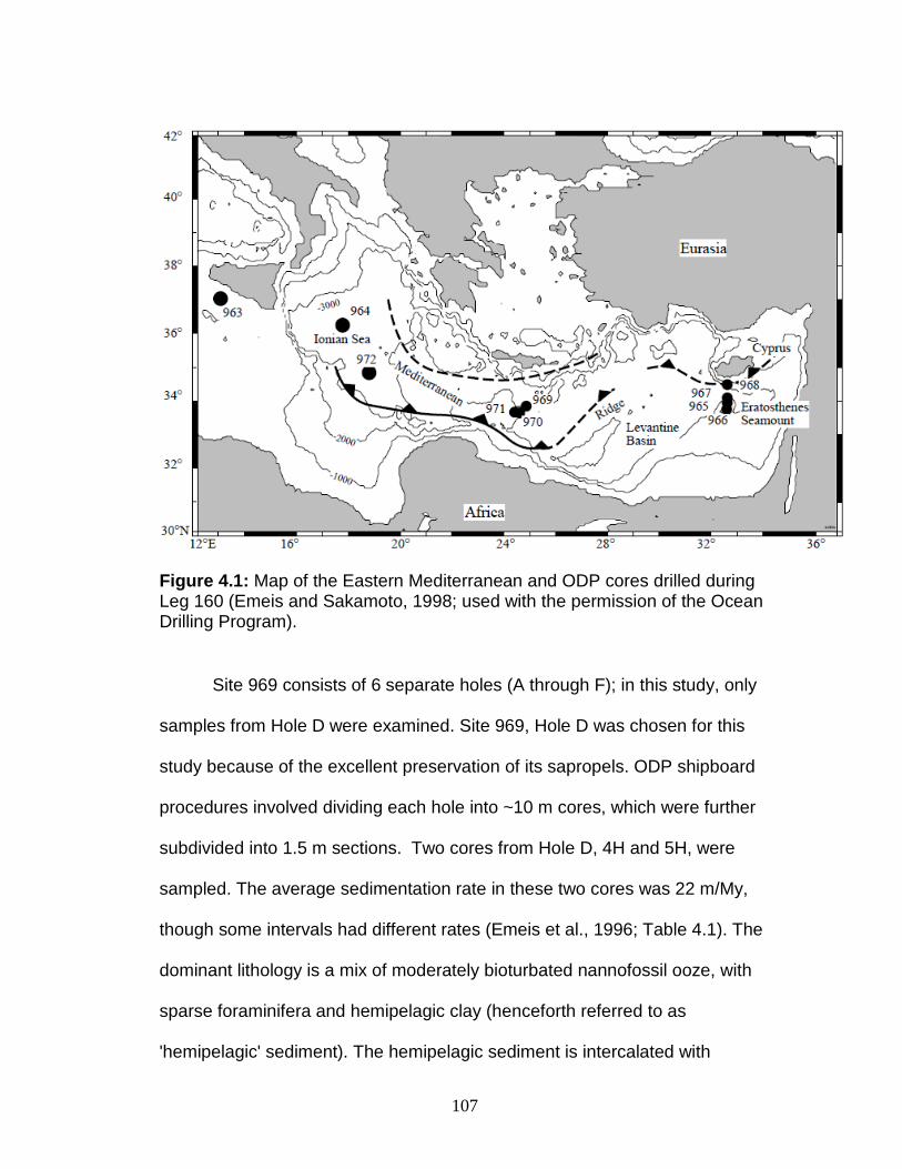
107

Figure 4.1: Map of the Eastern Mediterranean and ODP cores drilled during Leg 160 (Emeis and Sakamoto, 1998; used with the permission of the Ocean Drilling Program).

Site 969 consists of 6 separate holes (A through F); in this study, only

samples from Hole D were examined. Site 969, Hole D was chosen for this

study because of the excellent preservation of its sapropels. ODP shipboard

procedures involved dividing each hole into ~10 m cores, which were further

subdivided into 1.5 m sections. Two cores from Hole D, 4H and 5H, were

sampled. The average sedimentation rate in these two cores was 22 m/My,

though some intervals had different rates (Emeis et al., 1996; Table 4.1). The

dominant lithology is a mix of moderately bioturbated nannofossil ooze, with

sparse foraminifera and hemipelagic clay (henceforth referred to as

'hemipelagic' sediment). The hemipelagic sediment is intercalated with

108

organic-rich sapropel layers. The sapropel layers in both these cores display

fine laminations and internal color gradations that can be seen in core photos

(Emeis et al., 1996, Appendix 2). In some intervals of hemipelagic

sedimentation, extensive reddish layers are apparent, which are though to be

the oxidized remains of former sapropels, completely erased by 'burn-down'

diagenesis (Emeis et al., 2000), but sometimes retaining a portion of the

organic and trace-element rich nature of the precursors (Thomson et al.,

1995).

Age model

Assuming the orbitally-driven nature of their deposition, age tuning to

an eccentricity-modulated precessional index allows for good precision in

ages (±500 yr, Emeis et al., 2000). The middle of each sapropel was

assigned an age by Emeis et al. (2000), adapted from the orbital insolation

(astronomical) age model of Lourens et al. (1998; Table 4.2). Those ages

were determined based on the La90(1,1) summer insolation curve at 65°N

(Laskar et al., 1993). The insolation ages themselves are based on

cyclostratigraphic tuning to the Laskar et al. (1993) astronomical insolation

record, with a 3000 year lag incorporated into the ages (Lourens et al., 1998;

Emeis et al., 2000). In this work, the sapropel mid-point ages of Emeis et al.,

(2000), were used to linearly interpolate ages for the remaining samples (Fig.

4.2), using sedimentation rates from Emeis et al. (1996).

109

Sampling strategy

The samples record about 420 thousand years of deposition, and span

the Pliocene-Pleistocene boundary (1.45 to 1.87 Ma, Table 4.2). More

closely-spaced samples were taken in the interval between 1.44 and 1.47 Ma.

This interval, thus, has much higher temporal resolution than the samples

between 1.48 and 1.87 Ma. The strategy behind the high-temporal resolution

samples was to investigate incremental changes in sapropel properties, and

thus, in the depositional conditions, over a single sapropel. In contrast, the

low temporal resolution samples were intended to provide details about the

broader range of potential depositional modes for sapropels in the

Mediterranean. All the samples are ~1 cm thick plugs, each of which samples

~500 years of deposition, which is less than the resolution of the age model.

Table 4.1: Sedimentation rates, in meters/million years (m/My) for intervals of core 969D used to calculate ages (Emeis et al., 1996). Start End Sed. Rate (m /My) 4H-2, 40 4H-3, 20 33.6 4H-3, 20 4H-4, 27 29.6 4H-4, 27 4H-5, 95 21.7 4H-5, 95 5H-1, 50 6.4 5H-1, 50 5H-4, 20 22.1

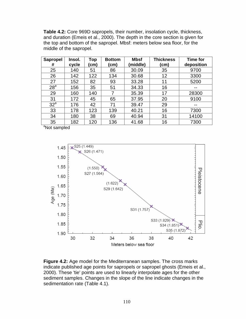
110

Table 4.2: Core 969D sapropels, their number, insolation cycle, thickness, and duration (Emeis et al., 2000). The depth in the core section is given for the top and bottom of the sapropel. Mbsf: meters below sea floor, for the middle of the sapropel. Sapropel

# Insol. cycle

Top (cm)

Bottom (cm)

Mbsf (middle)

Thickness (cm)

Time for deposition

25 140 51 86 30.09 35 9700 26 142 122 134 30.68 12 3300 27 152 82 93 33.28 11 5200 28a 156 35 51 34.33 16 -- 29 160 140 7 35.39 17 28300 31 172 45 65 37.95 20 9100 32a 176 42 71 39.47 29 -- 33 178 123 139 40.21 16 7300 34 180 38 69 40.94 31 14100 35 182 120 136 41.68 16 7300

aNot sampled

Figure 4.2: Age model for the Mediterranean samples. The cross marks indicate published age points for sapropels or sapropel ghosts (Emeis et al., 2000). These 'tie' points are used to linearly interpolate ages for the other sediment samples. Changes in the slope of the line indicate changes in the sedimentation rate (Table 4.1).

111

High temporal resolution sampling across a single sapropel (S25)

A single sapropel (I-140, Sapropel #25, samples 4H-2, 54 through 4H-

2, 84), which is ~30 cm thick, was sampled at 2-cm intervals, with occasional

4-cm spacing.The deposition of the entire sapropel took ~9700 years (Table

4.2). The advent of sapropel deposition (4H-2, 98 through 4H-2, 88) and the

return to hemipelagic sedimentation (4H-2, 40 and 51) were also closely

sampled. The deposition of S25 was briefly interrupted after ~6500 years (20

cm), resulting in an ~2000 y (~7 cm) hiatus during which hemipelagic

sediments were deposited. The hiatus has been interpreted to be the result of

a brief renewal of convective mixing of sufficient intensity to overcome the

chemical titration of oxygen by reduced compounds (Rohling et al., 2006;

Scrivner et al., 2004). Convective mixing might have occurred as a result of a

brief dry period that interrupted the monsoon maximum, resulting in cooling

surface water conditions; an idea which is supported for Holocene-aged

"interrupted" sapropels (e.g., Rohling et al., 2006; Scrivner et al., 2004). After

the hiatus, sapropel deposition then continued for a further ~1200 y (3 cm)

interval. Emeis et al. (2000), considered the total unit as a single sapropel.

Low temporal resolution samples

This aspect of the study examines samples from seven different

sapropel layers. Two samples were taken adjacent to one another in two of

these sapropels. Hemipelagic sediments were sampled at random intervals,

and several were taken in areas of the core where reddish pigmentation was

noted (Emeis et al., 1996). One sample (4H-6, 40) is a 'ghost' sapropel,

112

which is a former sapropel where the organic carbon has been completely

oxidized.

Analytical Methods All the samples were prepared by first crushing to a fine powder in a

ceramic mortar, and then combusting at 500° C in a furn ace for ~5 hours, in

order to rid the sample of organic carbon. Combustion at this temperature

does not result in a loss of Mo or Re, nor does it change the Mo isotopic

composition (Scheiderich et al., 2010). Small subsamples of powder were

dissolved and spiked with a 97Mo spike, in order to determine preliminary Mo

concentrations. These measurements were made by single-collector ICP-MS.

For determination of isotopic composition and final concentrations, the

samples were weighed into Teflon Savillex beakers and an appropriate

amount of a 97Mo-100Mo double spike solution was weighed and added.

Dissolution was accomplished by adding concentrated distilled acids (HCl,

HNO3, HCLO4, and HF) and heating to 90° on a hot plate. In the case of the

hemipelagic samples, which are carbonate-rich, the spiked sample was

transferred to a clean centrifuge tube, and shaken with 1-2 ml of 1M HCl until

all the carbonate was reacted. 3-4 ml of distilled H2O was added and the

sample was centrifuged. This solution was drawn off, transferred to a clean

beaker, dried, then reconstituted in 6M HCl. The remaining solid sample was

then digested with HF. After the HF step, the solution was returned to the

digested sample. This method circumvents the difficulty of using HF to

accomplish a bulk dissolution of Ca-rich samples, where appreciable amounts

113

of insoluble CaF will form, and possibly sequester Mo. This method was

tested by analyzing comparing it to the same samples processed via a bulk

method (Chapter 2). Resulting isotopic values and concentrations were

identical within analytical uncertainties. Once fully dissolved, Mo was

separated from matrix using an anion exchange column, followed by a cation

exchange column. Often a third column was necessary to complete the

separation; this column was a small version of the initial anion column. Details

of the bulk dissolution and chromatographic procedures are described in

Chapter 2. For each set of samples, one of two in-house rock standard

reference materials was also processed and analyzed. These data are

provided in Chapter 2. Duplicate samples are shown in Appendix 2. The

concentration errors from the double-spike method were a maximum of ~4%,

and the 2-s.d. error for Mo isotope analyses is ±0.1‰, based on long-term

reproducibility of the two in house reference materials. The Mo blank

averaged 3 ng, which comprised less than a tenth of 1% of total Mo extracted

from any sample, and was inconsequential for all samples.

Combusted powder was sub-sampled for Re concentration analysis via

isotope dilution. This was accomplished by adding a 185Re spike to small

quantities (<0.1 g) of bulk sample, and dissolving them. The Re

chromatographic separation procedure is described in Morgan and Walker

(1989). The Re blank was <10 pg and was insignificant for all samples. Errors

on Re concentrations are ±1% or better. All Mo and Re measurements were

114

performed using a Nu Plasma MC-ICP-MS, coupled with an ESI Apex

desolvating nebulizer for sample introduction.

Major and select minor element analysis was performed on

uncombusted sample material by X-ray fluorescence (Phillips 2402 XRF

vacuum spectrometer) at Franklin and Marshall College, PA. Approximate

uncertainties for XRF analysis in this lab are ±1% for major elements and

±5% for minor elements (Boyd and Mertzman, 1987). Detection limits for Co,

Cr, and V are 1-2 µg/g, for Sr and Zr, 0.5 µg/g, and for Ba 5 µg/g. Detection

limits for major elements are 0.02 g/kg (Marques et al., 2004).

Total organic carbon (TOC) was determined on µg quantities of

uncombusted, carbonate-free sapropel. The carbonate was eliminated from

the sample by reaction with 1M HCl. Once all the carbonate was dissolved,

the sample was dried, and the requisite amount weighed into an aluminum

boat. The analyses were performed on a Micromass Isoprime continuous flow

mass spectrometer. Errors for TOC are ≤0.3%, based on reproducibility for

repeated analyses of an organic carbon standard.

A small subset of sapropel and hemipelagic samples were processed

and analyzed for multiple sulfur isotopes. The methods for separation of sulfur

phases and subsequent analysis of sulfur isotopes are described in Appendix

2. All data are normalized to V-Canyon Diablo Troilite (V-CDT), and δ34S is

further normalized to Mediterranean seawater sulfate.

115

Results Molybdenum isotope data, V, and Re concentrations, and Mo/Al, Fe/Al

and Mn/Al ratios are plotted, relative to age, in Figures 4.3 and 4.4. The plots

are separated into high-resolution (1.44 to 1.47 Ma) and low-resolution (1.48

to 1.90 Ma) for clarity. In these figures, Mo/Al ratios, Fe/Al, and Mn/Al are

plotted in order to illustrate variations in an element relative to terrigenous

concentrations. For these samples, Al is controlled by terrigenous input, so

normalizing to Al eliminates the effects of trace element dilution by carbonate

as well as opal (Nijenhuis et al., 1999; Lyons et al., 2003). The ranges of V,

Re, Mo/Al, Fe/Al, Mn/Al, and δ98Mo values, are illustrated for both

hemipelagic and sapropel samples in Figs. 4.5 and 4.6. Noteworthy aspects

of these parameters include the large range of δ98Mo values (4‰) in

hemipelagic material, and the smaller range present in the sapropels (1.8‰).

116

Figure 4.3: The high-temporal resolution sampling across S25. The green layer represents the sapropel, whereas the brown layers encompass samples whose geochemistry is most likely influenced by proximity to the sapropel. Hemipelagic intervals are indicated by the blocked background.

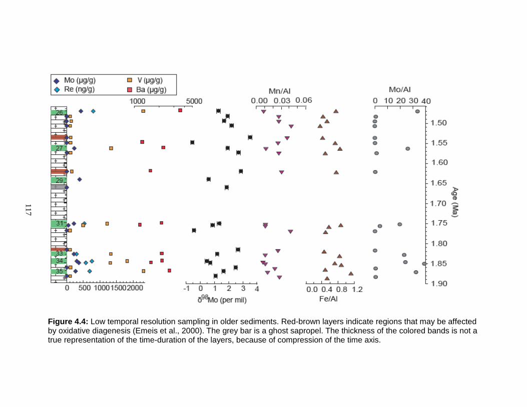
117

Figure 4.4: Low temporal resolution sampling in older sediments. Red-brown layers indicate regions that may be affected by oxidative diagenesis (Emeis et al., 2000). The grey bar is a ghost sapropel. The thickness of the colored bands is not a true representation of the time-duration of the layers, because of compression of the time axis.

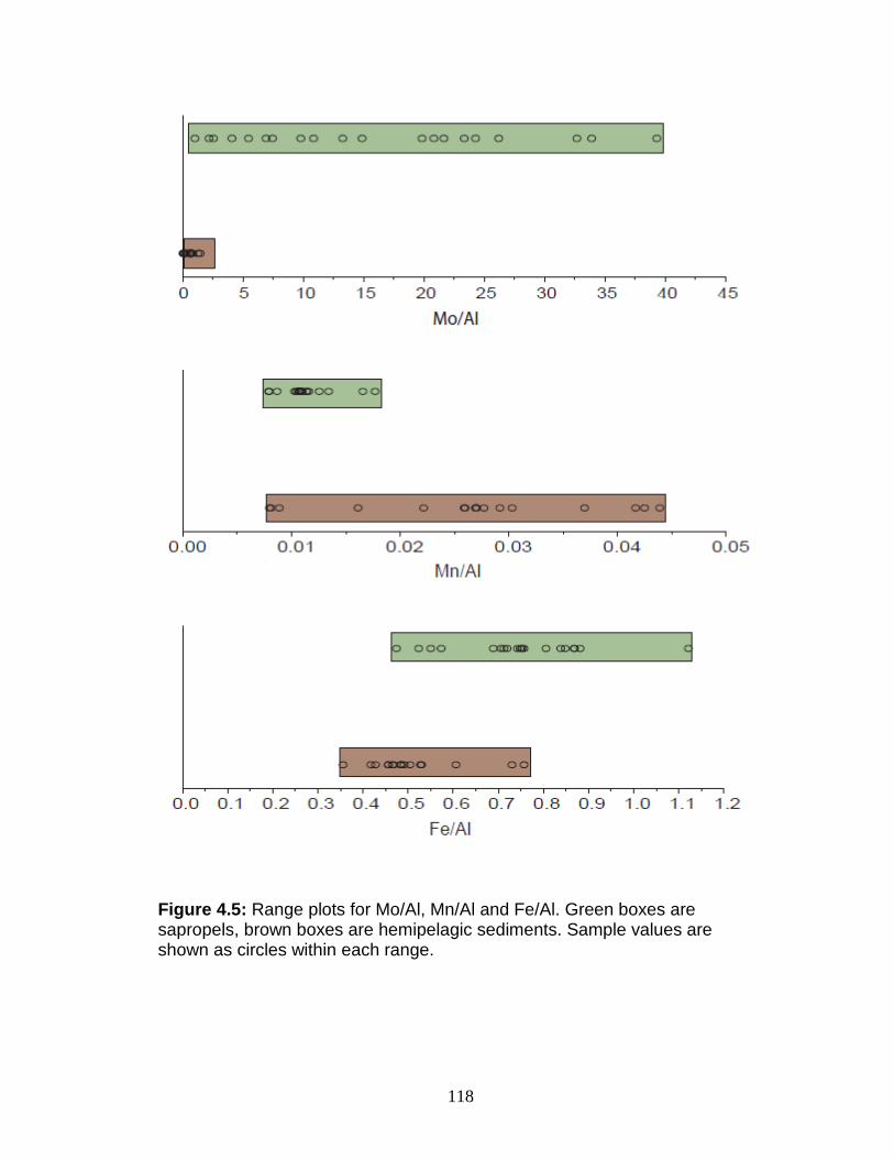
118

Figure 4.5: Range plots for Mo/Al, Mn/Al and Fe/Al. Green boxes are sapropels, brown boxes are hemipelagic sediments. Sample values are shown as circles within each range.

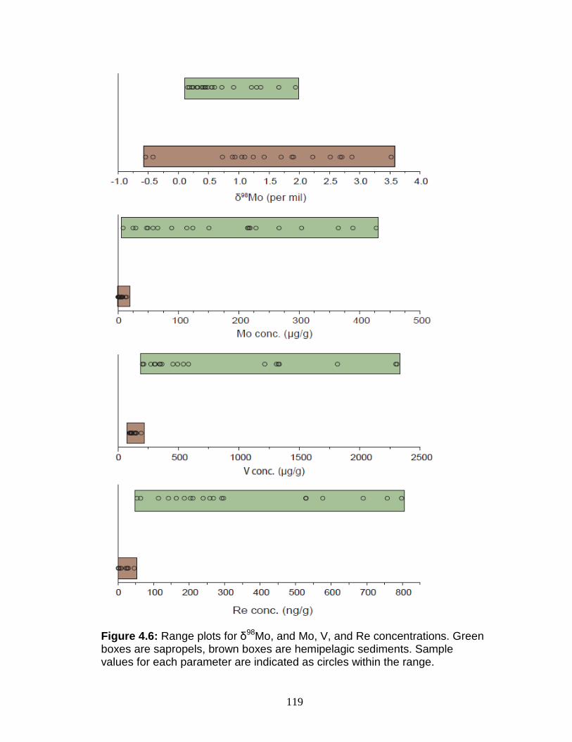
119

Figure 4.6: Range plots for δ98Mo, and Mo, V, and Re concentrations. Green boxes are sapropels, brown boxes are hemipelagic sediments. Sample values for each parameter are indicated as circles within the range.

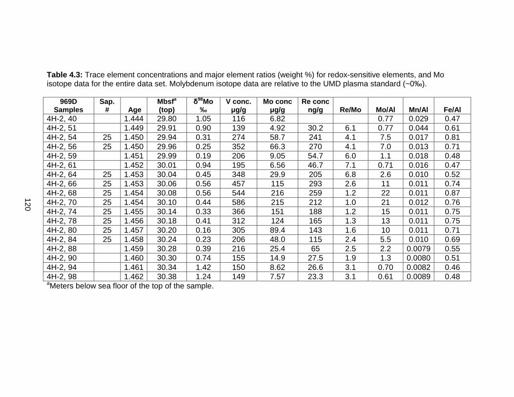
120

Table 4.3: Trace element concentrations and major element ratios (weight %) for redox-sensitive elements, and Mo isotope data for the entire data set. Molybdenum isotope data are relative to the UMD plasma standard (~0‰).

969D Samples

Sap. # Age

Mbsf a (top)

δ98Mo ‰

V conc. µg/g

Mo conc µg/g

Re conc ng/g Re/Mo Mo/Al Mn/Al Fe/Al

4H-2, 40 1.444 29.80 1.05 116 6.82 0.77 0.029 0.47 4H-2, 51 1.449 29.91 0.90 139 4.92 30.2 6.1 0.77 0.044 0.61 4H-2, 54 25 1.450 29.94 0.31 274 58.7 241 4.1 7.5 0.017 0.81 4H-2, 56 25 1.450 29.96 0.25 352 66.3 270 4.1 7.0 0.013 0.71 4H-2, 59 1.451 29.99 0.19 206 9.05 54.7 6.0 1.1 0.018 0.48 4H-2, 61 1.452 30.01 0.94 195 6.56 46.7 7.1 0.71 0.016 0.47 4H-2, 64 25 1.453 30.04 0.45 348 29.9 205 6.8 2.6 0.010 0.52 4H-2, 66 25 1.453 30.06 0.56 457 115 293 2.6 11 0.011 0.74 4H-2, 68 25 1.454 30.08 0.56 544 216 259 1.2 22 0.011 0.87 4H-2, 70 25 1.454 30.10 0.44 586 215 212 1.0 21 0.012 0.76 4H-2, 74 25 1.455 30.14 0.33 366 151 188 1.2 15 0.011 0.75 4H-2, 78 25 1.456 30.18 0.41 312 124 165 1.3 13 0.011 0.75 4H-2, 80 25 1.457 30.20 0.16 305 89.4 143 1.6 10 0.011 0.71 4H-2, 84 25 1.458 30.24 0.23 206 48.0 115 2.4 5.5 0.010 0.69 4H-2, 88 1.459 30.28 0.39 216 25.4 65 2.5 2.2 0.0079 0.55 4H-2, 90 1.460 30.30 0.74 155 14.9 27.5 1.9 1.3 0.0080 0.51 4H-2, 94 1.461 30.34 1.42 150 8.62 26.6 3.1 0.70 0.0082 0.46 4H-2, 98 1.462 30.38 1.24 149 7.57 23.3 3.1 0.61 0.0089 0.48 aMeters below sea floor of the top of the sample.

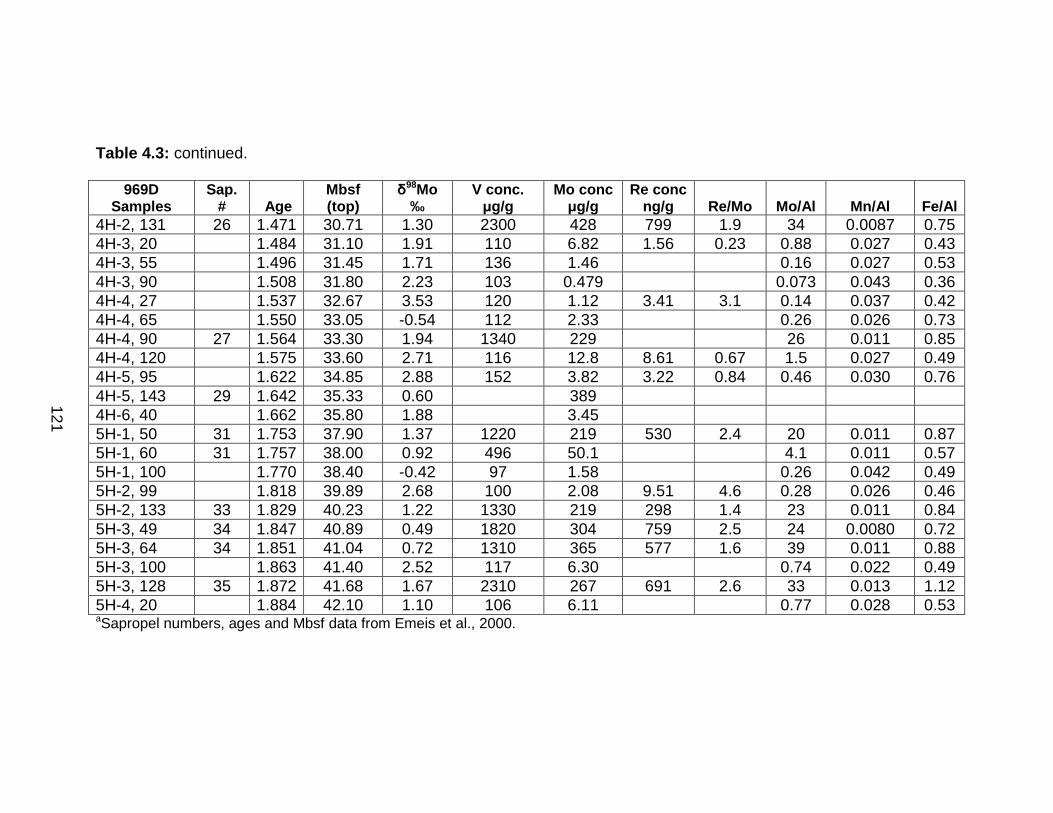
121

Table 4.3: continued.

969D Samples

Sap. # Age

Mbsf (top)

δ98Mo ‰

V conc. µg/g

Mo conc µg/g

Re conc ng/g Re/Mo Mo/Al Mn/Al Fe/Al

4H-2, 131 26 1.471 30.71 1.30 2300 428 799 1.9 34 0.0087 0.75 4H-3, 20 1.484 31.10 1.91 110 6.82 1.56 0.23 0.88 0.027 0.43 4H-3, 55 1.496 31.45 1.71 136 1.46 0.16 0.027 0.53 4H-3, 90 1.508 31.80 2.23 103 0.479 0.073 0.043 0.36 4H-4, 27 1.537 32.67 3.53 120 1.12 3.41 3.1 0.14 0.037 0.42 4H-4, 65 1.550 33.05 -0.54 112 2.33 0.26 0.026 0.73 4H-4, 90 27 1.564 33.30 1.94 1340 229 26 0.011 0.85 4H-4, 120 1.575 33.60 2.71 116 12.8 8.61 0.67 1.5 0.027 0.49 4H-5, 95 1.622 34.85 2.88 152 3.82 3.22 0.84 0.46 0.030 0.76 4H-5, 143 29 1.642 35.33 0.60 389 4H-6, 40 1.662 35.80 1.88 3.45 5H-1, 50 31 1.753 37.90 1.37 1220 219 530 2.4 20 0.011 0.87 5H-1, 60 31 1.757 38.00 0.92 496 50.1 4.1 0.011 0.57 5H-1, 100 1.770 38.40 -0.42 97 1.58 0.26 0.042 0.49 5H-2, 99 1.818 39.89 2.68 100 2.08 9.51 4.6 0.28 0.026 0.46 5H-2, 133 33 1.829 40.23 1.22 1330 219 298 1.4 23 0.011 0.84 5H-3, 49 34 1.847 40.89 0.49 1820 304 759 2.5 24 0.0080 0.72 5H-3, 64 34 1.851 41.04 0.72 1310 365 577 1.6 39 0.011 0.88 5H-3, 100 1.863 41.40 2.52 117 6.30 0.74 0.022 0.49 5H-3, 128 35 1.872 41.68 1.67 2310 267 691 2.6 33 0.013 1.12 5H-4, 20 1.884 42.10 1.10 106 6.11 0.77 0.028 0.53 aSapropel numbers, ages and Mbsf data from Emeis et al., 2000.

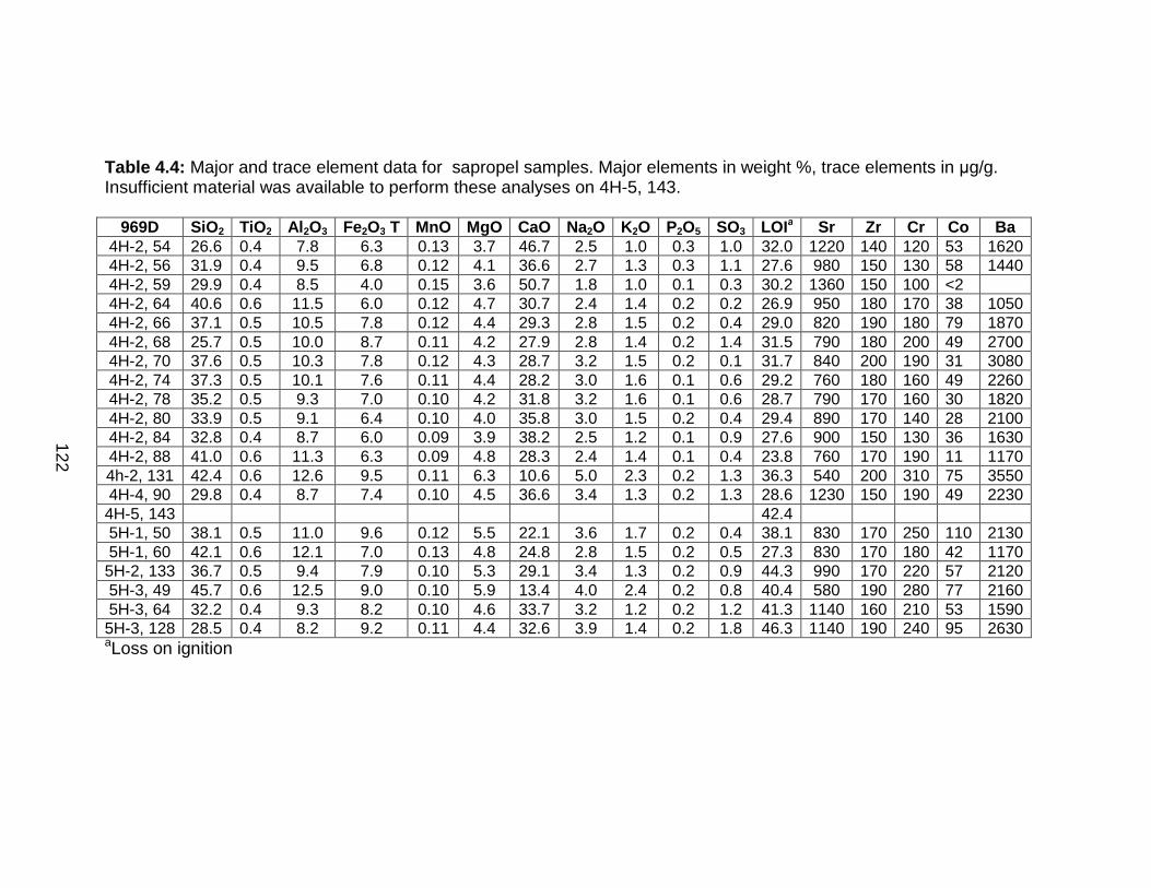
122

Table 4.4: Major and trace element data for sapropel samples. Major elements in weight %, trace elements in µg/g. Insufficient material was available to perform these analyses on 4H-5, 143.

969D SiO2 TiO2 Al 2O3 Fe2O3 T MnO MgO CaO Na2O K2O P2O5 SO3 LOIa Sr Zr Cr Co Ba 4H-2, 54 26.6 0.4 7.8 6.3 0.13 3.7 46.7 2.5 1.0 0.3 1.0 32.0 1220 140 120 53 1620 4H-2, 56 31.9 0.4 9.5 6.8 0.12 4.1 36.6 2.7 1.3 0.3 1.1 27.6 980 150 130 58 1440 4H-2, 59 29.9 0.4 8.5 4.0 0.15 3.6 50.7 1.8 1.0 0.1 0.3 30.2 1360 150 100 <2 4H-2, 64 40.6 0.6 11.5 6.0 0.12 4.7 30.7 2.4 1.4 0.2 0.2 26.9 950 180 170 38 1050 4H-2, 66 37.1 0.5 10.5 7.8 0.12 4.4 29.3 2.8 1.5 0.2 0.4 29.0 820 190 180 79 1870 4H-2, 68 25.7 0.5 10.0 8.7 0.11 4.2 27.9 2.8 1.4 0.2 1.4 31.5 790 180 200 49 2700 4H-2, 70 37.6 0.5 10.3 7.8 0.12 4.3 28.7 3.2 1.5 0.2 0.1 31.7 840 200 190 31 3080 4H-2, 74 37.3 0.5 10.1 7.6 0.11 4.4 28.2 3.0 1.6 0.1 0.6 29.2 760 180 160 49 2260 4H-2, 78 35.2 0.5 9.3 7.0 0.10 4.2 31.8 3.2 1.6 0.1 0.6 28.7 790 170 160 30 1820 4H-2, 80 33.9 0.5 9.1 6.4 0.10 4.0 35.8 3.0 1.5 0.2 0.4 29.4 890 170 140 28 2100 4H-2, 84 32.8 0.4 8.7 6.0 0.09 3.9 38.2 2.5 1.2 0.1 0.9 27.6 900 150 130 36 1630 4H-2, 88 41.0 0.6 11.3 6.3 0.09 4.8 28.3 2.4 1.4 0.1 0.4 23.8 760 170 190 11 1170 4h-2, 131 42.4 0.6 12.6 9.5 0.11 6.3 10.6 5.0 2.3 0.2 1.3 36.3 540 200 310 75 3550 4H-4, 90 29.8 0.4 8.7 7.4 0.10 4.5 36.6 3.4 1.3 0.2 1.3 28.6 1230 150 190 49 2230 4H-5, 143 42.4 5H-1, 50 38.1 0.5 11.0 9.6 0.12 5.5 22.1 3.6 1.7 0.2 0.4 38.1 830 170 250 110 2130 5H-1, 60 42.1 0.6 12.1 7.0 0.13 4.8 24.8 2.8 1.5 0.2 0.5 27.3 830 170 180 42 1170 5H-2, 133 36.7 0.5 9.4 7.9 0.10 5.3 29.1 3.4 1.3 0.2 0.9 44.3 990 170 220 57 2120 5H-3, 49 45.7 0.6 12.5 9.0 0.10 5.9 13.4 4.0 2.4 0.2 0.8 40.4 580 190 280 77 2160 5H-3, 64 32.2 0.4 9.3 8.2 0.10 4.6 33.7 3.2 1.2 0.2 1.2 41.3 1140 160 210 53 1590 5H-3, 128 28.5 0.4 8.2 9.2 0.11 4.4 32.6 3.9 1.4 0.2 1.8 46.3 1140 190 240 95 2630 aLoss on ignition

123

Table 4.5: Major and trace element data for hemipelagic samples. Major elements in weight %, trace elements in µg/g. Insufficient material was available to perform these analyses on 4H-6, 40.

969D SiO2 TiO2 Al 2O3 Fe2O3 T MnO MgO CaO Na2O K2O P2O5 SO3 LOIa Sr Zr Cr Co Ba

4H-2, 40 30.3 0.46 8.9 4.2 0.26 3.3 49.9 1.7 0.9 0.2 0.3 30.4 1570 180 79 <2 4H-2, 51 22.3 0.28 6.4 3.9 0.28 2.9 62.1 1.3 0.6 0.2 0.2 34.4 1770 130 72 10 4H-2, 61 32.7 0.44 9.3 4.4 0.15 3.8 45.3 1.8 1.2 0.1 0.2 28.3 1220 150 120 10 4H-2, 90 40.6 0.56 11.2 5.7 0.09 4.6 29.6 2.1 1.3 0.1 0.4 22.4 820 170 160 8 1210 4H-2, 94 43.6 0.61 12.2 5.6 0.10 4.6 26.0 2.1 1.8 0.1 0.4 21.5 900 190 130 6 440 4H-2, 98 43.9 0.63 12.3 6.0 0.11 4.5 25.2 2.2 1.7 0.1 0.7 21.2 870 200 110 2 430 4H-3, 20 26.5 0.39 7.8 3.3 0.21 3.4 54.1 1.9 1.2 0.2 0.4 31.1 1680 160 63 <2 4H-3, 55 31.9 0.42 8.9 4.7 0.24 4.0 44.0 2.1 1.3 0.1 0.4 28.1 1350 150 120 <2 4H-3, 90 23.3 0.32 6.6 2.4 0.28 3.3 61.7 1.2 0.7 0.2 0.1 34.9 1750 140 61 <2 4H-4, 27 27.8 0.38 7.8 3.3 0.29 3.7 54.0 1.4 0.9 0.2 0.2 32.4 1530 150 84 <2 4H-4, 65 30.7 0.45 8.8 6.5 0.23 3.4 44.7 1.6 0.7 0.2 0.5 24.8 1430 170 94 <2 1240 4H-4, 120 31.1 0.42 8.5 4.1 0.23 3.7 48.8 1.8 0.9 0.2 0.5 29.9 1520 170 64 <2 4H-5, 95 29.3 0.38 8.2 6.2 0.25 4.4 42.9 2.1 1.3 0.2 0.8 21.9 1150 120 110 3 1560 4H-6, 40 26.0 5H-1, 100 22.8 0.30 6.0 3.0 0.25 3.4 62.1 1.6 0.7 0.3 0.1 28.6 1730 140 54 <2 5H-2, 99 27.4 0.37 7.3 3.4 0.19 3.4 55.8 1.5 0.7 0.2 0.1 31.5 1690 160 82 <2 5H-3, 100 31.5 0.43 8.6 4.2 0.19 3.4 47.9 1.8 1.0 0.2 0.2 29.2 1610 180 69 <2 5H-4, 20 27.5 0.38 7.9 4.2 0.22 3.3 53.3 1.8 1.1 0.2 0.3 30.9 1440 180 65 <2

aLoss on ignition

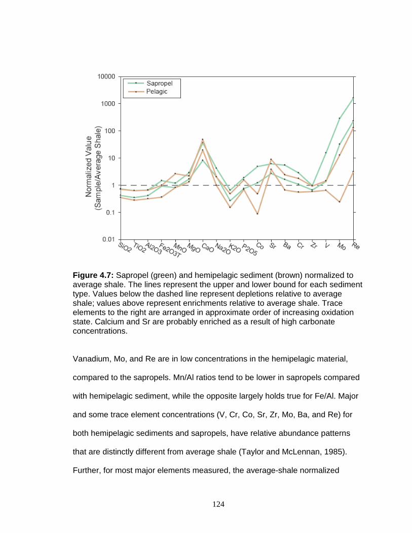
124

Figure 4.7: Sapropel (green) and hemipelagic sediment (brown) normalized to average shale. The lines represent the upper and lower bound for each sediment type. Values below the dashed line represent depletions relative to average shale; values above represent enrichments relative to average shale. Trace elements to the right are arranged in approximate order of increasing oxidation state. Calcium and Sr are probably enriched as a result of high carbonate concentrations.

Vanadium, Mo, and Re are in low concentrations in the hemipelagic material,

compared to the sapropels. Mn/Al ratios tend to be lower in sapropels compared

with hemipelagic sediment, while the opposite largely holds true for Fe/Al. Major

and some trace element concentrations (V, Cr, Co, Sr, Zr, Mo, Ba, and Re) for

both hemipelagic sediments and sapropels, have relative abundance patterns

that are distinctly different from average shale (Taylor and McLennan, 1985).

Further, for most major elements measured, the average-shale normalized

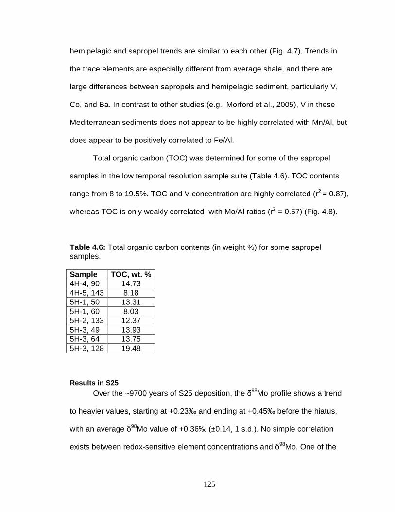
125

hemipelagic and sapropel trends are similar to each other (Fig. 4.7). Trends in

the trace elements are especially different from average shale, and there are

large differences between sapropels and hemipelagic sediment, particularly V,

Co, and Ba. In contrast to other studies (e.g., Morford et al., 2005), V in these

Mediterranean sediments does not appear to be highly correlated with Mn/Al, but

does appear to be positively correlated to Fe/Al.

Total organic carbon (TOC) was determined for some of the sapropel

samples in the low temporal resolution sample suite (Table 4.6). TOC contents

range from 8 to 19.5%. TOC and V concentration are highly correlated (r2 = 0.87),

whereas TOC is only weakly correlated with Mo/Al ratios (r2 = 0.57) (Fig. 4.8).

Table 4.6: Total organic carbon contents (in weight %) for some sapropel samples. Sample TOC, wt. % 4H-4, 90 14.73 4H-5, 143 8.18 5H-1, 50 13.31 5H-1, 60 8.03 5H-2, 133 12.37 5H-3, 49 13.93 5H-3, 64 13.75 5H-3, 128 19.48

Results in S25

Over the ~9700 years of S25 deposition, the δ98Mo profile shows a trend

to heavier values, starting at +0.23‰ and ending at +0.45‰ before the hiatus,

with an average δ98Mo value of +0.36‰ (±0.14, 1 s.d.). No simple correlation

exists between redox-sensitive element concentrations and δ98Mo. One of the

126

hemipelagic samples from the sapropel hiatus has a heavier δ98Mo value than

the associated sapropel, and most of these hemipelagic sediment samples have

δ98Mo values that are heavier than those in S25.

Beginning ~6 cm below the sapropel proper, concentrations of redox-

sensitive elements start to increase above the sediment background. All of the

redox-sensitive elements are most concentrated in the upper-middle part of S25.

The relative enrichment for V concentrations is much less than for Re and Mo,

but generally follow the same pattern. Barium is significantly enriched in the

sapropel (Figs. 4.3 and 4.4). During the oxic hiatus, Fe/Al, Mo/Al, and Re

concentrations return to background values before increasing again during the

renewal of sapropel deposition. Mn/Al is relatively constant (0.01 to 0.02)

throughout most of S25, but there is a marked increase to 0.04 just after S25

deposition ends. However, crustal ratios of 0.06 are not attained.

Results in the sediments between 1.48 and 1.90 Ma

The sapropels in this older sequence have δ98Mo values that are much

more variable than those in S25. Two sapropels (S34 and S29) have values that

are within the range of S25, but other samples are generally heavier, with δ98Mo

between +0.9 and +1.9‰. The TOC data are loosely correlated with δ98Mo

values and Mo/Al. Many of the older sapropels have larger enrichments in V, Re,

Ba, Mo/Al, and Fe/Al, compared with S25.

The hemipelagic samples exhibit mostly heavy δ98Mo values, between

+1.1 and +3.5‰. Two samples have very light δ98Mo values (-0.4 and -0.5‰). All

127

the samples have relatively low concentrations of V, Mo, Re, and low Fe/Al. Most

show enrichments in Mn/Al compared to the sapropel layers.

Figure 4.8: Positive correlation, in the older sapropels, between TOC and V concentration (squares), and between TOC and Mo/Al (green circles).

Discussion The Eastern Mediterranean during sapropel deposition can be compared

to the Black Sea, a 'type locality' for euxinic deposition. The Black Sea has been

extensively studied with respect to the hydrologic controls operating in the basin,

and the effects on redox-sensitive element behavior. Such a comparison

provides a context in which to place the Mediterranean sediments.

Hydrographically, the two basins differ in a number of features, the first being that

128

the Black Sea circulation is estuarine. This results from the much lower salinity of

the surface waters (~18 psu, Colodner et al., 1995) relative to the hypersaline

input from the Mediterranean. The Black Sea has been permanently euxinic

below 100 m depth since ~7500 years ago (Ryan et al., 1997), while the modern

Mediterranean is well ventilated at all depths (Malanotte-Rizzoli and Robinson,

1992), but experienced anoxic, possibly sulfidic conditions during sapropel

events as recently as 7000 years ago.

In general, the Mediterranean sapropels are much richer in the redox-

sensitive elements (V, Re, Mo, and Ba) than Black Sea sapropels (e.g.,

Brumsack 1989; Ravizza et al., 1991; Nägler et al., 2005), which has also been

noted by other studies (Rinna et al., 2002; Warning and Brumsack, 2000). Fe/Al

ratios in the Mediterranean sapropels and hemipelagic sediment are similar to

those from euxinic and oxic Black Sea sediments (Lyons and Severmann, 2006).

The average Re/Mo ratio in the Black Sea sapropels (Ravizza et al., 1991;

Warning and Brumsack, 2000) is lower than the average in Mediterranean

sapropels (1.5 vs. 3.7). Lastly, in the Black Sea, Mo isotope fractionation occurs

along the gradient of H2Saq levels (-0.6 to +2.0‰; oxic sediments ~+0.2‰), until

the switch point is reached, whereupon sediments reflect a δ98Mo value close to

seawater (~+2.3±0.2‰; Nägler et al., 2005; Neubert et al., 2008; Arnold et al.,

2004). The consensus with respect to the Black Sea is that high sulfide levels in

the water column, below 400 m, lead to nearly complete scavenging of redox-

sensitive elements from the water column.

129

Redox-sensitive element concentrations

The V, Re, Mo, and Ba concentrations and Fe/Al ratios in S25 appear to

track the slow onset of water-column conditions necessary for sapropel

deposition (Fig. 4.3). These parameters all begin to increase above the

background values at about 6 cm below the sapropel. This might indicate an

increased degree of scavenging from the water column. Alternatively, diffusion

of sulfide out of the sapropel after its deposition might have increased the

diagenetic fixation of these elements (Rinna et al., 2002). These parameters

reach a peak in the middle to upper portion of S25, which could reflect the most

intense reducing conditions in

the water column. After the hiatus, V, Re, and Mo do not again reach as high

concentrations as in the main portion of S25, suggesting that suboxic conditions

dominated.

Many of the older sapropels (S26, S27, S34, S35) have all the indicators

of high degrees of oxygen depletion: high Mo, Re, and V concentrations, and

high TOC, Fe/Al, and Mo/Al. These examples have 2 to 4 times as much V as

S25, and higher Re and Mo concentrations, suggesting that different depositional

conditions may have obtained. Vanadium and TOC are highly correlated in

these samples (Fig. 4.8), as a result of V being strongly associated with organic

carbon (e.g., Emerson and Huested, 1991). Mo/Al and TOC are less well

correlated (Fig. 4.8), possibly because Mo removal may be positively controlled

by the amount of sulfide (HS-) produced in organic carbon-rich sediments

(Crusius et al., 1996; Helz et al., 1996; Erickson and Helz, 2000; Lyons et al.,

2000).

130

Fe/Al in Mediterranean sediments

Fe/Al ratios are another proxy for the state of the water column during

deposition, Fe/Al between 0.6 and 1.2 characterizes euxinic conditions, ratios

between 0.5-0.6 indicate more oxic deposition (Lyons and Severmann, 2006).

Iron deposited on oxic shelf environments will be remobilized, until it eventually

moves into the deep euxinic water where it can be fixed as pyrite, enriching the

euxinic sediments relative to the oxic sediments (Lyons and Severmann, 2006).

Fe/Al can also reflect Fe enrichment through formation of Fe-oxyhydroxide

phases, when euxinic conditions are not present (Lyons and Severmann, 2006).

In sediments immediately surrounding sapropels, post-depositional diagenesis

can result in formation of FeOx phases can form from oxidized pyrite (Larrasoana

et al., 2003).

The average Fe/Al of sapropels in this study is 0.75 (± 0.15, 1σ); by the

Lyons and Severmann (2006) scheme these values are well within the euxinic

range. However, the light δ98Mo values differ from expectations for sediments

deposited under such conditions (Fig. 4.9). The discrepancy may be related to

higher Fe input to the basin during sapropel formation, consistent with

hypotheses of increased nutrient fluxes (Rossignol-Strick et al., 1982; Rohling

and Gieskes, 1989; Thomson et al., 1995). However, the Fe/Al ratios do indicate

an overall O2 depleted system.

δ98Mo of Mediterranean sediments

There are two particularly striking features in this data set. The first is the

wide range in δ98Mo within organic-rich layers that presumably formed under low-

131

O2 conditions, coupled with the fact that few of the values approach the

presumed δ98Mo of Mediterranean seawater (~+2.3‰). This is particularly

striking when compared with the consistency of the sapropel δ98Mo values from

the Black Sea.

The second unusual feature in the sample set is the even larger range of

δ98Mo values that are evident in the hemipelagic ooze deposited between

sapropel episodes, and the very heavy δ98Mo in many of these samples. It might

be expected that these sediments, deposited under oxic conditions, would have

light δ98Mo values consistent with any of the following processes: addition of

detrital Mo (~0‰), removal to MnOx (δ98Mo = -0.8 to -0.‰, Barling and Anbar,

2004, Wasylenki et al., 2008), or removal to FeOx (-0.4 to +1.3‰, Goldberg et al.,

2009). MnOx, in particular, is a significant carrier of Mo in oxic oceanic sediments

(Bertine and Turekian, 1973). However, while many of these samples have Mn/Al

ratios greater than those in the sapropels, only two samples have δ98Mo values

typical of MnOx-rich sediments. FeOx phases may dominate over MnOx in marine

sediments (Poulton and Raiswell, 2002), and can also adsorb large amounts of

Mo (Gustafsson, 2003). Thus, the range of fractionation seen within the

hemipelagic sediments may be partly a result of adsorption to FeOx (Goldberg et

al., 2009). Indeed, in the Black Sea, oxic hemipelagic sediments are significantly

lighter (-0.1 to +0.3‰) than the sapropel above them (Nägler et al., 2005;

Neubert et al., 2008). Thus, the

132

Figure 4.9: Top: Fe/Al versus Mo isotopic composition. Bottom: Fe/Al versus Mo/Al. Symbols as in previous figures (brown for hemipelagic sediments, dark green for S25 and pale green for older sapropels).

133

positive values in the Mediterranean oxic sediments are contradictory to the

prevailing view about how δ98Mo values are controlled in the oceans. In order to

explain these two features, two general classes of mechanism are considered.

The first class includes mechanisms that utilize a different source of Mo during

sapropel versus hemipelagic deposition. The second class invokes variable

fractionation mechanisms of Mo from the same source material, probably

seawater, during the two times.

Variable Mo sources

Two possibilities for a Mo source other than seawater will be discussed.

The first of these possibilities involves the upward diffusion of Mo-rich brine from

buried Messinian salt deposits. Evaporative processes may enrich a brine in

trace elements, particularly Mo, and result in δ98Mo in brines similar to, or heavier

than, seawater (Ryb et al., 2009). It has been argued that upward brine migration

contributed to the salinity of the modern Mediterranean (van Santvoort, 1996).

However, several observations are inconsistent with the idea that the Mo in

sapropels was delived by an Mo-rich brine. An upward-migrating brine would

have to move through ~70 m of sediment, through which other sapropels are

distributed. It would likely lose any Mo that it carried as soon as it encountered

sulfidic pore water. Secondly, and more importantly, an upward-moving front

might be expected to yield the heaviest δ98Mo values near the bottom of a profile,

with values decreasing smoothly towards the top as a result of diffusive

fractionation. However, the profile shows both light and heavy values in the lower

and upper sapropels, probably ruling out a brine-related mechanism.

134

The second possibility for variably-sourced Mo is a change in the δ98Mo of

surface seawater during sapropel deposition, stemming from freshwater influx.

The δ98Mo of the sapropels could be set by scavenging of Mo in the highly

productive surface waters. Both Mo isotope and trace-element mass-balance

calculations provide arguments against a significant change in the δ98Mo of

seawater during sapropel deposition.

The dilution of ambient seawater with Nile freshwater of a different isotopic

composition could affect the δ98Mo of the Mediterranean, and thus, of sapropels

forming under euxinic or anoxic conditions. To test this, a simple conservative

linear mixing calculation was performed, using the Mo concentrations and δ98Mo

values of Nile river water (Archer and Vance, 2008). It is necessary to assume

that Pliocene-Pleistocene oceanic δ98Mo was similar to today's +2.3‰ (Siebert et

al., 2003). Futher description of the calculation and a plot of the results of the

calculation are given in Appendix 2. In order to significantly change the isotopic

composition of the Eastern Mediterranean through freshwater addition alone, the

mix would require >80% freshwater, because the Mo concentration in river water

is low (<1.4 µg/L) compared to seawater.

It is possible to assess the likely sources of V, Mo, and Re to the

sapropels, and to determine whether the Eastern Mediterranean was entirely

restricted during sapropel deposition (Nijenhuis et al. (1999). The total amount of

metal, in kg, in a sapropel deposited over an area of 2/3 of the Eastern

Mediterranean is calculated (Table 4.7). Using the volume of the Eastern

Mediterranean, the total amount of metal (in kg) available in the basin is also

135

calculated. Using the deposition rate of the sapropel, and metal concentration,

the rate of removal of each element can be calculated. Different potential trace

element sources are manipulated to determine the time required to satisfy the

sapropel metal 'demand' with that source. These sources are: Nile river influx

increased by factors of 1.5 and 10; Nile influx increased by 1.5 plus Black Sea

water; and exchange with Western Mediterranean seawater. The concentration

parameters for seawater, Nile river water and Black Sea water are given in Table

4.8. The flow parameters are further described in Appendix 2. In the calculations

using river water and Black Sea water, the time to deliver the requisite metal

quantities is many times longer than the duration of sapropel deposition (Table

4.7). However, seawater satisfies the trace element quantities, even at an

exchange rate decreased by a factor of 10.

Furthermore, if seawater was the source, then circulation between the

Eastern Mediterranean and Western Mediterranean cannot have shut down

completely, or the effect would be seen as a sudden decrease in trace-metal

concentration across the sapropel. The amount of time required to completely

deplete the Eastern Mediterranean in V, Mo and Re, given isolation of the deep

water, and removal at the calculated rates, is given in the last column. In most

cases, the times are shorter than the duration of sapropel deposition, yet no

sudden decrease is seen in the trace element profiles (Fig. 4.3).

Thus, either scavenging was incomplete (but probably high), or circulation

continued between the two basins. A scenario of limited circulation is consistent

with evidence for reduced ventilation during formation of some sapropels (e.g.,

136

Casford et al., 2003; Larrasoana et al., 2003), because the vast quantities of

sinking organic matter would rapidly deplete the new deep water mass of O2

(e.g., Rohling, 1994). Support for incomplete scavenging can be seen in the

profile of δ98Mo in S25. The near constant values suggest that the δ98Mo of the

source water was not changing during sapropel deposition.

Variable Mo fractionation mechanisms

The degree of variability between sapropels and hemipelagic sediments

suggests a fractionation process within the water column or pore water, or

possibly a diagenetic resetting of the δ98Mo values after burial, as was observed

for Holocene Mediterranean sapropels (Reitz et al., 2007). Sapropels frequently

experience post-depositional oxidative diagenesis (e.g., Thomson et al, 1995;

Jung et al., 1996). During such a process, Mo could be fractionated during

uptake to oxic authigenic phases such as MnOx (Reitz et al., 2007) or FeOx.

Thus, it is important to determine whether the sapropels in this study were

'burned down'. It has been argued that Ba is the trace element that is least

susceptible to this effect, and is, therefore, the best indicator of the original extent

of a sapropel (Thomson et al., 1995; Wehausen and Brumsack, 2000). Profiles of

Ba and Mo concentrations suggest that S25 did not experience an oxidation front

(Figs. 4.3 and 4.4).

Previous studies have reported conditions under which isotopic

fractionation of Mo relative to seawater could occur in the water column: 1)

anoxic margins, where δ98Mo of +1.6‰ have been reported (Poulson et al.,

2006), 2) 'suboxic' water columns where δ98Mo has been observed to range from

137

-0.5 to +1.6 (e.g., Siebert et al., 2006), 3) variably sulfidic water columns below,

and up to, the quantitative switch point (Erickson and Helz, 2000), where δ98Mo

has been observed to range between -0.6 and +2.4‰ (Neubert et al., 2008), and

4) in oxic sediments, uptake of Mo by MnOx and FeOx can significantly

fractionate Mo from seawater values (Barling and Anbar, 2004, Wasylenki et al.,

2008; Goldberg et al., 2009).

In a previous study of Mo isotopes in a Mediterranean sapropel, it was

found that the δ98Mo values could be attributed to dissolution of MnOx and

delivery of light δ98Mo to the pore water, which could then be fixed as

thiomolybdates below the redox boundary (Reitz et al., 2007). Such a hypothesis

seems less likely in this case, because there is a distinct difference: geochemical

evidence suggests that the Eastern Mediterranean was intermittently ventilated

during S1 deposition (Casford et al., 2003), whereas most of the evidence

presented thus far indicates suboxic water column conditions during deposition of

S25, and anoxic conditions for most of the older sapropels. Development of

MnOx layers during sapropel deposition is, thus, unlikely. As further support for

the lack of a MnOx role in the δ98Mo values of S25, Mn/Al ratios are consistently

low. A peak in Mn/Al just above the sapropel most likely indicates the depth of

the redox boundary in the sediments at some time after sapropel deposition had

ceased. The peak in the Mo profile is not coincident with the Mn peak,

suggesting that Mn dissolution and Mo enrichment are not related.

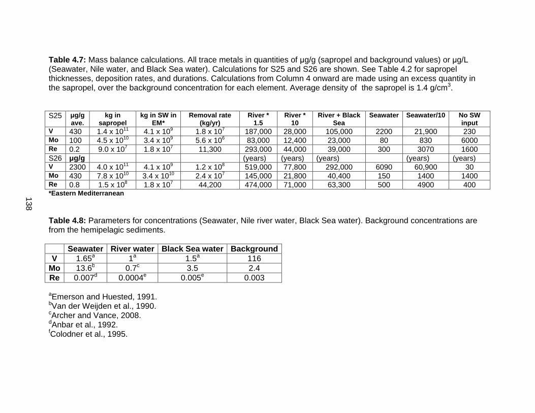
138

Table 4.7: Mass balance calculations. All trace metals in quantities of µg/g (sapropel and background values) or µg/L (Seawater, Nile water, and Black Sea water). Calculations for S25 and S26 are shown. See Table 4.2 for sapropel thicknesses, deposition rates, and durations. Calculations from Column 4 onward are made using an excess quantity in the sapropel, over the background concentration for each element. Average density of the sapropel is 1.4 g/cm3. S25 µg/g

ave. kg in

sapropel kg in SW in

EM* Removal rate

(kg/yr) River *

1.5 River *

10 River + Black

Sea Seawater Seawater/10 No SW

input V 430 1.4 x 1011 4.1 x 109 1.8 x 107 187,000 28,000 105,000 2200 21,900 230 Mo 100 4.5 x 1010 3.4 x 109 5.6 x 106 83,000 12,400 23,000 80 830 6000 Re 0.2 9.0 x 107 1.8 x 107 11,300 293,000 44,000 39,000 300 3070 1600 S26 µg/g (years) (years) (years) (years) (years) V 2300 4.0 x 1011 4.1 x 109 1.2 x 108 519,000 77,800 292,000 6090 60,900 30 Mo 430 7.8 x 1010 3.4 x 1010 2.4 x 107 145,000 21,800 40,400 150 1400 1400 Re 0.8 1.5 x 108 1.8 x 107 44,200 474,000 71,000 63,300 500 4900 400 *Eastern Mediterranean Table 4.8: Parameters for concentrations (Seawater, Nile river water, Black Sea water). Background concentrations are from the hemipelagic sediments. Seawater River water Black Sea water Background V 1.65a 1a 1.5a 116

Mo 13.6b 0.7c 3.5 2.4 Re 0.007d 0.0004e 0.005e 0.003 aEmerson and Huested, 1991. bVan der Weijden et al., 1990. cArcher and Vance, 2008. dAnbar et al., 1992. fColodner et al., 1995.

139

Delivery of isotopically light Mo from MnOx dissolution could, nonetheless,

have affected the total isotopic composition of S25. In order to generate the

observed values, assuming a euxinic water column and complete drawdown from

seawater (+2.3‰) and a δ98MoMnOx of -0.7‰, 60% of the Mo would need to be

delivered from MnOx. Other sapropels would need a smaller contribution from

MnOx in order to attain their isotopic compositions.

Overall, however, invoking mixing of diagenetic MnOx-derived Mo is

unsatisfying as a way to impart the observed isotopic compositions, because of

the lack of Mn/Al enrichments in the sapropels that would indicate delivery of

isotopically light Mo. There is no correlation between Mn/Al ratio and δ98Mo, nor

between Mn/Al and Mo concentrations or Mo/Al. MnOx reduction typically

happens at such shallow sediment depths that much of the Mn, and presumably

any released Mo, or V, can be lost to the bottom water (Morford et al., 2005).

Suboxic and anoxic deposition generate distinctive ranges of Mo isotopic

compositions. In Fig. 4.10, these ranges are laid out with respect to the

measured bottom water content (Siebert et al., 2006; Poulson et al., 2006), and

the Mediterranean data are binned according to the ranges. The largest number

of sapropel samples fall into ranges that are consistent with deposition under low,

variable degrees of oxygenation. However, the majority of the hemipelagic

samples also are encompassed by ranges consistent with lower oxygen,

suggesting the possibility that the oxic water column of the Pliocene was less

140

oxic than the modern Mediterranean, and that therefore hemipelagic deposition

was also occurring under a 'suboxic' water column.

A suboxic/anoxic mechanism for the δ98Mo values in the sapropel is

problematic in one respect. The observed enrichments in trace metals are at

odds with previous studies identifying only small enrichments (<10 µg/g) under

bottom water O2 of 5 µM or less (e.g., Zheng et al., 2000; Nameroff et al., 2002).

Fractionation of Mo during formation of thiomolybdate intermediates (Tossell,

2005) provides a possible explanation for the entire range of δ98Mo values in the

sapropels. This mechanism occurs under varying concentrations of H2Saq

(Erickson and Helz, 2000), as suggested by Neubert et al. (2007), for Black Sea

sediments. Such a process generates a similar range of values to those for

suboxic deposition, as noted by Neubert et al., but high redox-sensitive element

concentrations are more easily reconciled with a model where low oxygen

coexists with low sulfide.

A scenario to generate sulfide and create low bottom water O2 can be

envisioned. Oxidation of high quantities of sinking organic carbon probably

contributed to deep water O2 depletion (e.g., Rohling and Hilgen, 1991), while

bacterial sulfate reduction in the forming sapropel, and subsequent outward

diffusion of the generated H2S, may have created a sulfidic layer above the

sediments (Passier et al., 1997). The concentration and thickness of the H2Saq

layer above the sediments would be temporally variable, dependant on rates of

deep water advection, and the balance between organic matter delivery, sulfate

reduction, and reactive Fe supply. Molybdate in the water column, upon

141

Figure 4.10: The number of samples from this study that fall into the specified δ98Mo range. The corresponding number of hemipelagic (P) and sapropels (S) in each range is given below. P(g) refers to 'ghost' sapropels, samples that were sapropels, but have been diagenetically erased . These ranges correspond to bottom water (BW) oxygen contents (Siebert et al., 2006; Poulson et al., 2006).

exposure to the sulfidic layer, would commence formation of thiomolybdate,

along the sequence dictated by [H2Saq] (Erickson and Helz, 2000). Thus, Mo

would fractionatate from the initial seawater δ98Mo (+2.3‰) according to the

particular species of thiomolybdate formed (Tossell, 2005). Slow advection of

WM bottom water with δ98Mo = 2.3‰ might ensure that the isotopic composition

of the source pool does not change significantly with time.

142

One possible complication in this concept is that molybdate reaching the

sulfidic layer may already be fractionated, as a result of association with organic

matter. Available evidence (Liermann et al., 2005; Wasylenki et al., 2007)

suggests that biological utilization of Mo would result in net lighter Mo reaching

the sulfidic layer, and budget calculations suggest an -0.1‰ offset from seawater

(Poulson-Brucker et al., 2009). In such a case, the thiomolybdates that formed

under higher [H2Saq] would necessarily appear lighter than seawater. Thus,

organic matter fractionation prior to thiomolybdate formation does not present a

difficulty with respect to the observed values in the sapropels.

A partial-fractionation model is successful at explaining the entire range of

δ98Mo data observed in the sapropel sediments, from 'suboxic' values to anoxic

values, and some that approach 'euxinic'. The δ98Mo data bear out previous

hypotheses that the conditions for sapropel formation were different for each

individual event. For sapropels with suboxic/ partially fractionated thiomolybdate

signatures, the conditions may not have progressed beyond weakened

circulation and lessened bottom water ventilation (e.g., Stratford et al., 2000),

while for the anoxic sapropels, circulation reversal and isolation of the deep water

may be more likely.

Sulfur isotope systematics in 969D Sulfur isotopes from sapropels might be useful in determining whether the

water column was euxinic during sapropel formation. Sulfur isotope data and

uncertainties are listed in Table 4.9. The δ34S results in sedimentary pyrite from

this study are consistent with previous results (Passier et al., 1997). Modern

143

seawater sulfate in the Mediterranean has δ34S = +20.6‰ (De Lange et al.,

1990), thus the fractionation between seawater sulfate and sulfide in the

sediments can be calculated (Table 4.9). Seawater sulfate and sulfide in

hemipelagic sediments are fractionated from one another to the largest degree,

up to δ34S = -67‰. Fractionation between seawater sulfate and sulfide in the

sapropels is less than δ34S = -60‰ (Figure 4.11). In the sapropels, pyrite is

thought to form as a result of reaction of Fe with HS- (e.g., Passier et al., 1996;

Böttcher et al., 2003) produced by dissimilatory sulfate reducing prokaryotes.

During dissimilatory sulfate reduction, and sulfur disproportionation,

prokaryotic organisms generate distinctive isotope signatures in both δ34S and

∆33S that have been the focus of recent studies (e.g., Farquhar et al., 2003;

Johnston et al., 2005, 2007). These signatures result from the flow of sulfur

through the specific steps in the metabolism (Farquhar et al., 2003, 2007), and

provide additional information about fractionation at branch points between

reactants and products during the flow of S through the network (Farquhar et al.,

2003).

The structure of the sulfate reduction metabolism forms the basis for

interpretation of these isotopic signatures, and the isotopic fractionation

associated with sulfate reduction can be modeled using a metabolic network

approach (e.g., Rees, 1973; Brunner and Bernasconi, 2005; Farquhar et al.,

2007). Farquhar et al. (2007) calculated a field of δ34S and ∆33S values for sulfide

produced during the sulfate reduction metabolism, using the network of Brunner

and Bernasconi (2005) (Figure 4.12). This network expanded on the original

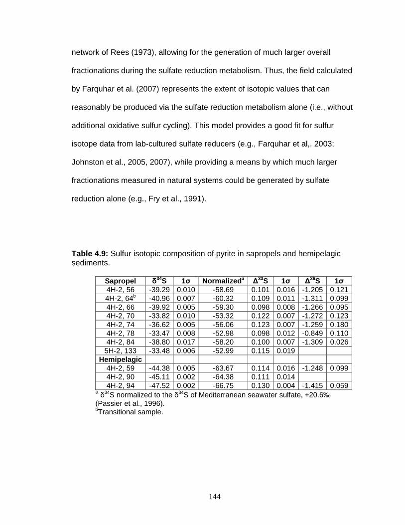
144

network of Rees (1973), allowing for the generation of much larger overall

fractionations during the sulfate reduction metabolism. Thus, the field calculated

by Farquhar et al. (2007) represents the extent of isotopic values that can

reasonably be produced via the sulfate reduction metabolism alone (i.e., without

additional oxidative sulfur cycling). This model provides a good fit for sulfur

isotope data from lab-cultured sulfate reducers (e.g., Farquhar et al,. 2003;

Johnston et al., 2005, 2007), while providing a means by which much larger

fractionations measured in natural systems could be generated by sulfate

reduction alone (e.g., Fry et al., 1991).

Table 4.9: Sulfur isotopic composition of pyrite in sapropels and hemipelagic sediments.

Sapropel δ34S 1σ Normalized a

∆33S 1σ ∆

36S 1σ 4H-2, 56 -39.29 0.010 -58.69 0.101 0.016 -1.205 0.121 4H-2, 64b -40.96 0.007 -60.32 0.109 0.011 -1.311 0.099 4H-2, 66 -39.92 0.005 -59.30 0.098 0.008 -1.266 0.095 4H-2, 70 -33.82 0.010 -53.32 0.122 0.007 -1.272 0.123 4H-2, 74 -36.62 0.005 -56.06 0.123 0.007 -1.259 0.180 4H-2, 78 -33.47 0.008 -52.98 0.098 0.012 -0.849 0.110 4H-2, 84 -38.80 0.017 -58.20 0.100 0.007 -1.309 0.026

5H-2, 133 -33.48 0.006 -52.99 0.115 0.019 Hemipelagic

4H-2, 59 -44.38 0.005 -63.67 0.114 0.016 -1.248 0.099 4H-2, 90 -45.11 0.002 -64.38 0.111 0.014 4H-2, 94 -47.52 0.002 -66.75 0.130 0.004 -1.415 0.059

a δ34S normalized to the δ34S of Mediterranean seawater sulfate, +20.6‰ (Passier et al., 1996). bTransitional sample.

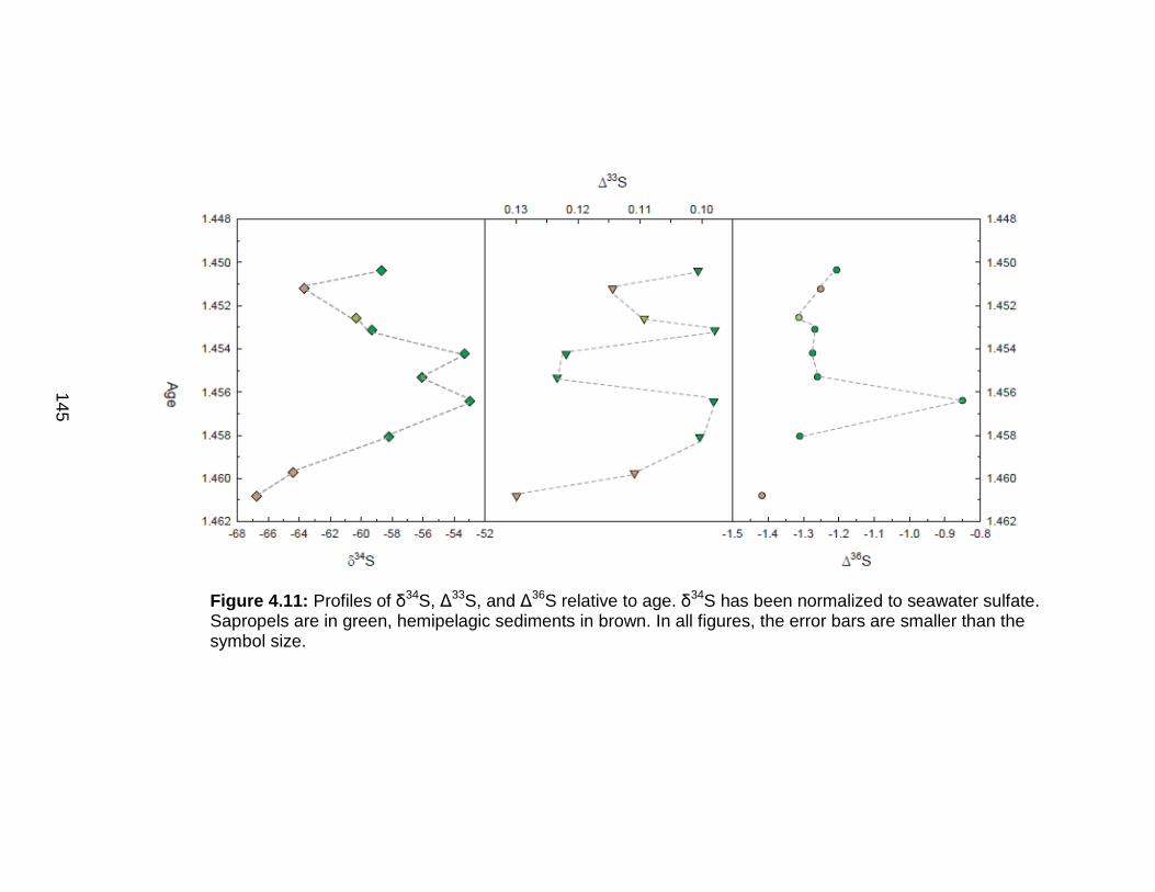
145

Figure 4.11: Profiles of δ34S, ∆33S, and ∆36S relative to age. δ34S has been normalized to seawater sulfate. Sapropels are in green, hemipelagic sediments in brown. In all figures, the error bars are smaller than the symbol size.

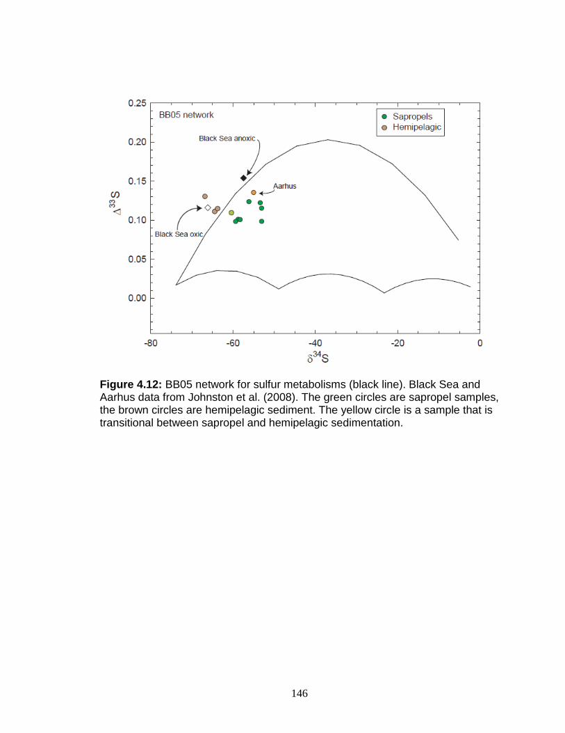
146

Figure 4.12: BB05 network for sulfur metabolisms (black line). Black Sea and Aarhus data from Johnston et al. (2008). The green circles are sapropel samples, the brown circles are hemipelagic sediment. The yellow circle is a sample that is transitional between sapropel and hemipelagic sedimentation.

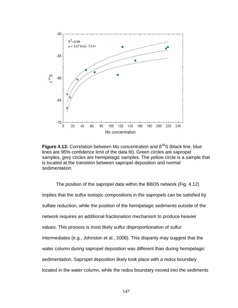
147

Figure 4.13: Correlation between Mo concentration and δ34S (black line, blue lines are 95% confidence limit of the data fit). Green circles are sapropel samples, grey circles are hemipelagic samples. The yellow circle is a sample that is located at the transition between sapropel deposition and normal sedimentation.

The position of the sapropel data within the BBO5 network (Fig. 4.12)

implies that the sulfur isotopic compositions in the sapropels can be satisfied by

sulfate reduction, while the position of the hemipelagic sediments outside of the

network requires an additional fractionation mechanism to produce heavier

values. This process is most likely sulfur disproportionation of sulfur

intermediates (e.g., Johnston et al., 2008). This disparity may suggest that the

water column during sapropel deposition was different than during hemipelagic

sedimentation. Sapropel deposition likely took place with a redox boundary

located in the water column, while the redox boundary moved into the sediments

148

at other times. A redox boundary in the sediments allows for oxidation of sulfide

to sulfur intermediates, which can be further fractionated by sulfur

disproportionating organisms.

A good logarithmic correlation (r2 = 0.88) exists between δ34S and Mo

concentration for all samples for which mutual data are available (Fig 4.13). The

highest Mo concentrations are coincident with the lightest δ34S values. Thus, high

degrees of Mo removal correlate with δ34S values that indicate an anoxic water

column above the forming sapropel. This strong positive relationship suggests

that Mo is related to δ34S through the connection with organic carbon

(Tribovillard et al., 2006, McManus et al., 2006; Lyons et al., 2003).

Molybdenum in hemipelagic sediments

An unexpected finding in the Mo isotope data is the predominant

occurrence of δ98Mo > 0.7‰ in the hemipelagic samples (Figs. 4.6 and 4.11),

which likely indicates deposition under low bottom water conditions. This

supports the idea that, for many of these samples, the Pliocene 'oxic' bottom

water was less oxygenated than the modern. Many of these also have Mo

concentrations much greater than crustal or shale averages. Because of MnOx

precipitation and diagenetic cycling, and contribution of continental material with

δ98Mo ~0‰ (Siebert et al., 2003), it would be expected that oxic sediments would

have little Mo, and be isotopically light. Indeed, oxic sediments from the Black

Sea have 0.8 to 1.0 µg/g Mo, and δ98Mo +0.1 to 0.3‰ (Nägler et al., 2005), while

a hemipelagic sample from the Holocene Mediterranean has 2.4 µg/g Mo and

δ98Mo +0.2 (Reitz et al., 2007). Oxidized remnants of a Mediterranean Holocene

149

sapropel had light δ98Mo values, down to -0.7‰ (Reitz et al., 2007). However, in

our study, several very heavy δ98Mo values (2.3 to 3.5‰), indicate an extreme

loss of light Mo, such as might occur by removal to a phase such as MnOx.

These values are similar to measurements of δ98Mo in pore-water, where Mo

removal to isotopically light authigenic phases enriched the pore fluid in heavy

Mo (McManus et al., 2002).

For almost all the hemipelagic samples, the proportion of detrital Mo

appears to be low, based on Mo/Al ratios. The Mo/Al ratio of average crust is

0.07 (Rudnick and Gao, 2003), and of average shale 0.08 (Taylor and

McLennan, 1985), and many of the hemipelagic samples have more than 10x

these ratios. Thus, contribution of a continental δ98Mo signature to the

hemipelagic sediments is probably negligible.

Foraminiferal and nannofossil carbonate is a major component of these

sediments. It was only recently recognized that carbonates can have a large

range of δ98Mo values (Voegelin et al., 2009). The inherent Mo concentration of

skeletal carbonate phases is low (on the order of 0.05 µg/g, Voegelin et al.,

2009), so carbonate-hosted Mo is unlikely to be significantly contributing to the

δ98Mo in the Mediterranean samples.

With the exception of two samples with δ98Mo values of -0.4 and -

0.5‰, contributions from MnOx can be ruled out. A δ98Mo signature similar to that

of MnOx adsorption can be generated through Mo adsorption to hematite, with a

minimum δ98Mo ~ -0.4‰ (Goldberg et al., 2009). The two hemipelagic samples

with negative δ98Mo values likely contain Mo that has been fractionated by

150

adsorption to MnOx or hematite, or both. The presence of small amounts of

magnetite in the background sediments and the oxidized layers above sapropels

(Larrasoana et al., 2003) could also have an effect on the δ98Mo of the

hemipelagic sediments. Molybdate diffusion into pore water and subsequent

adsorption to magnetite particles provides a possible explanation for some of the

hemipelagic sediments, in terms of both Mo concentration and isotopic

composition.

Pyrite is probably a carrier of Mo in sediments (Huerta-Diaz and Morse,

1992; Vorlicek and Helz, 2002). The fractionation of Mo during adsorption to or

scavenging by pyrite is unknown, but has been proposed to be the source of the

-0.7‰ offset of δ98Mo from seawater to anoxic, non-sulfidic sediments (Poulson

et al., 2006). Pyrite forms readily in the sapropels and adjacent sediments as a

result of sulfide diffusion from sapropels (e.g., Passier et al., 1996), and could

form in buried hemipelagic sediments that are below the redox boundary.

In the Black Sea, buried, formerly oxic sediments have Fe/Al <0.63 and low

degrees of pyritization (Lyons and Severmann, 2006). The Fe/Al ratio in most

969D hemipelagic samples is <0.53; a few samples have higher ratios. The

amount of Fe/Al suggests that pyrite, or certain FeOx phases forming in the

hemipelagic sediment, could be responsible for the δ98Mo values that are less

than seawater.

The source of isotopically very heavy Mo for some hemipelagic samples

remains to be identified. If the explanation for δ98Mo values in the sapropels is

partial fractionation during thiomolybdate formation, and suboxic/anoxic

151

conditions, then Mo remaining in pore water would become heavier. Diffusion of

this pool of Mo out of the sapropel region and into the hemipelagic sediments

satisfies the need for an isotopically heavy Mo source to form the observed

sediments. Where isotopically heavy hemipelagic samples are well removed

from a sapropel, diffusion of Mo into pore water, formation of isotopically lighter

phases, and diffusion of the heavy Mo pool to the redox boundary, where it could

be fixed, is a possible way to generate heavy δ98Mo signatures.

Collectively, the δ98Mo and trace metal evidence points to hemipelagic

depositional conditions that were similar to continental shelves or upwelling

zones (Siebert et al., 2006; Morford et al., 2005; Nameroff et al., 2002). Possibly,

the Eastern Mediterranean basin was subject to variations in ventilation, and was

on the whole less well-ventilated than it presently is during periods of

hemipelagic sedimentation. This suggest that the difference between sapropel

and hemipelagic episodes was the input of organic carbon, and not drastic shifts

in the degree of bottom water oxygenation caused by changes external to the

basin.

Rhenium/Molybenum ratios

The work of Crusius et al. (1996), presented the idea that the ratio of Re to

Mo in sediments could be used as an indicator of anoxic versus 'suboxic'

conditions. Samples with Re/Mo close to seawater (0.8 x 10-3) are indicative of

anoxic conditions, while higher ratios (>9 x 10-3) indicate suboxic deposition

(Crusius et al., 1996). Using Re/Mo to distinguish between between an anoxic

and a suboxic water column is theoretically possible because Re and Mo are

152

removed from seawater at different redox potentials (Crusius et al., 1996),

resulting in preferential enrichment of Re, relative to Mo, in suboxic sediments.

This implies that low levels of sediment oxidation (burn-down) might cause loss

of Re (Crusius and Thompson, 2000), before causing loss of Mo. In the Black

Sea, euxinic sediments have Re/Mo ratios from 0.7 to 2.1 (Ravizza et al., 1991).

If Re/Mo ratios of sapropel samples faithfully record information about the

oxygenation state of the water column during deposition, then the low Re/Mo

suggest that the sapropels examined here were likely deposited under relatively

reducing conditions (Fig. 4.14), in agreement with previous results for this site

(Warning and Brumsack, 2000; Rinna et al., 2002). For S25, Re/Mo ratios are

higher (more oxic) below the sapropel, and then transition gradually to Re/Mo

reflecting anoxic conditions in the center of the sapropel (Re/Mo = 1; Fig. 4.14).

The water column then evolves towards a ratio consistent with 'suboxic'

conditions, and during the hiatus, quite high ratios are present. The water column

appears to be more oxic during sapropel deposition following the hiatus (Re/Mo =

4.1). In the older sediments, Re/Mo is consistent with strongly anoxic conditions

in many of the sapropels (e.g., S33, Re/Mo = 1.4; S26 = Re/Mo 1.9). Within

hemipelagic samples, there is little consistency in Re/Mo. Ratios range between

7.1 and 0.2, with only one sample (4H-3, 20) displaying an 'oxic' (crustal) ratio

(~0.3; Zheng et al., 2000). This sample, however, has 3 times the abundance of

Re and Mo compared to average shale. Thus, the Re/Mo suggests that the

pelagic samples were also deposited under suboxic conditions, possibly under

conditions similar to modern suboxic regimes that have reported Re/Mo up to 19

153

(Crusius et al., 1996). Alternatively, the high pelagic ratios could be a function of

preferential Re addition to pore water during diagenetic oxygenation, while Mo is

retained in the sediments (Colodner et al., 1993). A return to anoxic pore water

conditions upon deeper burial could have preserved the diagenetic Re/Mo.

We suggest that Re/Mo indicates sapropel formation under both suboxic

and anoxic regimes, and hemipelagic sedimentation under varying oxygen levels.

However, there is a disconnect between the precise intervals that are designated

as anoxic or suboxic using Re/Mo, and those so indicated by the other data. The

δ98Mo values, particularly for S25, are 'suboxic' but have, for some of the

sequence Re/Mo ratios consistent with anoxic deposition. Conversely, the

sapropels identified as 'suboxic' by Re/Mo have δ98Mo values that are isotopically

heavy (+1 to +2‰), usually taken as an indicator of more reducing conditions.

154

Figure 4.14: Re/Mo ratios in sapropels and hemipelagic sediment. S25 is shown as the darker green circles, while the older sapropels are light green circles. The line which connects the S25 samples indicates the sequence of deposition (counter-clockwise).

In order to resolve this apparent decoupling, the Re concentrations alone

may be the key. If high Re alone is indicative of 'suboxic' conditions, then it might

correspond with suboxic δ98Mo values (Fig. 4.15). Rhenium concentrations in

S25 are lower compared with sapropels with more clearly anoxic signatures,

indicating that the Re concentrations and δ98Mo are in agreement with respect to

prevailing suboxic conditions during S25 deposition, and anoxic conditions in

older sapropels.

155

Thus, it remains to be answered why the Re/Mo is not faithfully recording

the state of the water column during sapropel formation. One possibility is that

the Re/Mo of Mediterranean water was changing with time during sapropel

deposition. Warning and Brumsack (2000) noted a decrease in average sapropel

Re/Mo with increasing distance from the seawater source, possibly as a result of

high Re and Mo removal rates to the sediments. This would affect Re more than

Mo, because of its lower concentration in seawater.

Another explanation comes from a comparison with the Black Sea.

Sulfidic conditions leading to incomplete scavenging of Mo might also lead to

partial scavenging of Re, in the same proportion. Thus, the ratio will reflect

seawater. In water column profiles from the Black Sea (Colodner et al., 1995),

scavenging of more than 75% of Re and Mo does not appear to greatly change

the dissolved Re/Mo ratio. Once sulfidic conditions are established in the water

column, the underlying sediments will carry a ratio that resembles seawater

regardless of the amount of scavenging. In the Mediterranean samples, then,

incomplete removal of Re and Mo at seawater ratios could be consistent with

partial isotopic fractionation of Mo during thiomolybdate formation. The larger

basin size and direct source of seawater in the Mediterranean allow for an overall

greater capacity to generate authigenic Re and Mo, compared to the Black Sea.

Incomplete scavenging of the Eastern Mediterranean water column would still

have the ability to deliver high quantities of trace elements to the sediments.

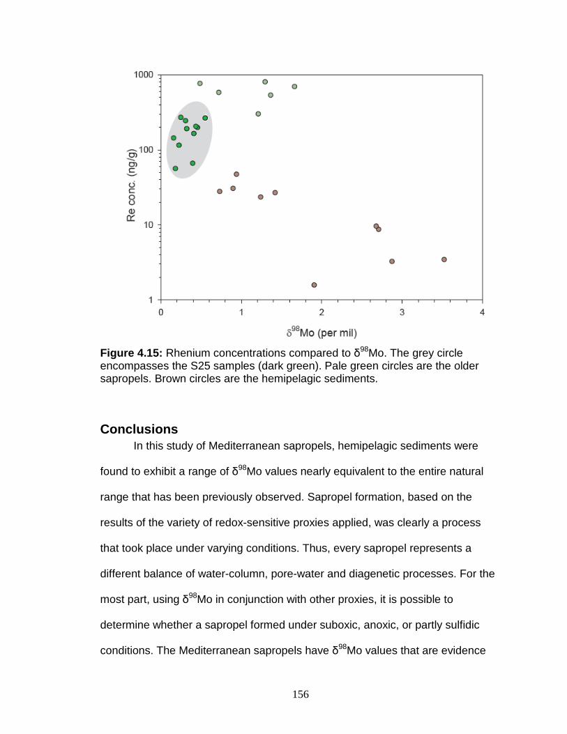
156

Figure 4.15: Rhenium concentrations compared to δ98Mo. The grey circle encompasses the S25 samples (dark green). Pale green circles are the older sapropels. Brown circles are the hemipelagic sediments.

Conclusions In this study of Mediterranean sapropels, hemipelagic sediments were

found to exhibit a range of δ98Mo values nearly equivalent to the entire natural

range that has been previously observed. Sapropel formation, based on the

results of the variety of redox-sensitive proxies applied, was clearly a process

that took place under varying conditions. Thus, every sapropel represents a

different balance of water-column, pore-water and diagenetic processes. For the

most part, using δ98Mo in conjunction with other proxies, it is possible to

determine whether a sapropel formed under suboxic, anoxic, or partly sulfidic

conditions. The Mediterranean sapropels have δ98Mo values that are evidence

157

for incomplete (fractionated) Mo removal, trace metal contents and Re/Mo ratios

that indicate high, but incomplete, degrees of scavenging from the water column.

δ98Mo values and other proxies from the hemipelagic samples indicate that the

degree of oxygenation during the Pliocene-Pleistocene was also variable, but

generally lower than in the modern Eastern Mediterranean.

The data for the sapropels suggest another important point: that Re/Mo

ratios cannot be relied upon to be a strict indicator of anoxic versus suboxic

depositional environment. We propose that high, but incomplete, degrees of

removal can generate Re/Mo ratios similar to seawater. This allows for high Re,

Mo and V concentrations and fractionated δ98Mo values to be coincident with

seawater Re/Mo, which could be misleading given the current paradigm.

158

Chapter 5: Experimental determination of Mo isotop e fractionation at high temperature and pressure

Abstract An experimental design that approximates a porphyry ore system at deep

crustal temperatures and pressures (800°C and 100 mPa) was used to assess

the fractionation of Mo isotopes between a vapor phase and a melt phase.

Molybdenum isotopic analysis of quenched run products was conducted using a

double-spike technique and multi-collector ICP-MS analysis. Resolvable

fractionation between vapor and melt was observed, with heavy Mo isotopes

favoring the vapor phase. Distribution coefficients of Mo indicate that Mo favors

the vapor phase, in agreement with previous results. A likely explanation for the

observed fractionation is that Mo undergoes a coordination change in the vapor,

which might explain the preference of heavy Mo isotopes for that phase.

Introduction A number of early Mo isotope studies included analyses of molybdenite

(MoS2), for its ease of processing and simple matrix (e.g., Anbar et al., 2001;

Barling et al., 2001). These studies reported a modest range in δ98Mo (-0.47 to

+0.27) for magmatic molybdenites, which might be expected for heavy element

fractionation in relatively high temperature systems (Urey, 1947). Further

studies, however, revealed a larger range with values from -0.77 to +2.27‰,

that appeared unrelated to the temperature or age of the deposit (Wieser and

DeLaeter, 2003; Pietruszka et al., 2006; Hannah et al., 2007; Malinovsky et al.,

2007). Two studies have systematically surveyed MoS2 deposits, and concluded

that there may be differences in δ98Mo that are related to the type of ore deposit

159

(Pietruszka et al., 2006; Mathur et al., 2009). Globally, porphyry systems exhibit

the largest range of values (-0.39 to +0.80‰), with samples from different parts

of the same deposit having highly variable δ98Mo (-0.24 to +0.51‰; Mathur et al.,

2009).

The use of Mo isotopes to study redox conditions of ancient ocean

environments has been predicated on assumptions about the behavior of Mo and

Mo isotopes in reduced and oxygenated environments, and about the isotopic

composition of input Mo. The ocean Mo reservoir is isotopically heavy (2.3‰),

and is though to reflect loss of isotopically light Mo to authigenic sediments under

oxic conditions. However, constraints on the δ98Mo of dissolved and particulate

material being delivered to the oceans are not well-developed. Studies of various

igneous rocks suggested the δ98Mo of the input is likely to be near 0‰ (Siebert et

al., 2001), but recent data for rivers show that δ98Mo in river water is highly

variable (Archer and Vance, 2008).

Input of large quantities of isotopically heavy molybdenite-derived Mo

might have the potential to change the ocean δ98Mo, introducing an uncertainty

to paleoredox studies. Such an effect would be more likely in localized settings,

such as enclosed seas, continental shelves proximal to uplifted areas, estuaries,

or lakes. Indeed, one instance of molybdenite weathering affecting δ98Mo and Mo

concentrations in lake sediments has already been identified (Malinovsky et al.,

2007).

Few laboratory studies have been conducted on Mo isotope behavior.

Most of these have focused on identifying the fractionation associated with Mo

160

removal to Mn and Fe oxides (Barling and Anbar, 2004; Wasylenki et al., 2008;

Goldberg et al., 2009), which are major components of sediments, and contribute

significantly to Mo removal from the ocean. Other fractionation factors have been

deduced from sediments themselves (McManus et al., 2002). The difficulty of

identifying a fractionation factor for MoS2 formation is the inability to link the

available molybdenite δ98Mo data with a specific mechanism, either temperature,

pressure, or fO2. One study has suggested that variations up to ~1‰ in MoS2

samples from a single occurrence could be explained by Rayleigh fractionation

from a vapor phase, but that the average isotopic composition of MoS2 from such

a deposit would be close to that of bulk continental crust (Hannah et al., 2007).

Molybdenum isotope data for the few igneous samples that have been measured

were interpreted to mean that high-temperature processes do not fractionate Mo

isotopes (Siebert et al., 2001). However, variations in Mo isotopic compositions

of a Hawaiian basalt, a MORB, and a Columbia river flood basalt suggests that

this may not always be true. These three materials have δ98Mo of -0.10, +0.08,

and +0.26, respectively (Scheiderich and Walker, unpublished data). No

experimental evidence has shown that Mo is fractionated during high-

temperature and/or high crustal pressure processes, such as might be present in

a hydrothermal ore system, where Mo(IV)S2 might form.

The goal of this study, therefore, is to experimentally determine the

magnitude and direction of Mo isotope fractionations among coexisting phases at

equilibrium conditions under high crustal temperatures and pressures. The

experimental system consisted of a vapor phase and a melt phase. Based on

161

equilibrium isotope fractionation theory (e.g., Schauble, 2004), the expectation

was that the vapor phase would become isotopically heavier, while the melt

phase would become lighter.

Molybdenite is a common sulfide mineral associated with porphyry-style

deposits, which are thought to be the result of magmatic-hydrothermal activity.

The source of the Mo in the magmas that give rise to some porphyry ore systems

is thought to be lower crustal rocks (Candela and Piccoli, 2005). Porphyry

deposits occur in a wide variety of tectonic settings, but the two main types of

porphyry Mo are rift-related (Climax-type) and subduction- related (Endako-type;

Sinclair, 2007). Ore metals are partitioned into a volatile phase within the magma

chamber, which accumulates at the apex of the chamber (e.g., Candela, 1989).

Vapor escapes into the overlying fractured rock, whereupon it cools to precipitate

ore minerals (Sinclair, 2007). This type of mineralization forms the basis for the

experimental design, which is a simple system consisting, at run conditions, of

co-existing vapor and melt phases. Molybdenum has been shown to more

favorable partition into the vapor phase relative to the melt (DMo >1, vapor-melt)

(Candela and Holland, 1984). At high temperature and pressure, Mo(VI)O3 has

been experimentally shown to be highly soluble in water vapor, possibly as a

result of hydration (Rempel et al., 2006), so in the vapor phase, Mo is likely

present as MoO3·nH2O (Rempel et al., 2009). At fO2 above the iron-wüstite

buffer, Mo(VI) is the dominant oxidation state in a silicate melt, and Mo is

probably present as molybdate, and to a smaller degree as molybdenyl (MoO66-)

moieties (Farges et al., 2006).

162

Experimental Methods The experimental design was as follows: 25 mm x 5 mm Au capsules

were loaded with materials that, under the run conditions, created a melt phase

and a Mo-containing vapor phase, allowing study of the fractionation of Mo

isotopes between these reservoirs. The experiments were designed so that all

had the same ratio of melt to vapor (0.4:1). 40 mg of a synthetic haplogranite

glass (GR-1, Qz: 0.38, Ab: 0.33, Or: 0.29) was used to generate the melt. GR-1

is the minimum melt composition for 100 MPa and 800°C. This material was

tightly packed into the capsule in order to minimize inclusion formation in the

melt. Its initial Mo content was below the detection limit of solution analysis by

single collector ICP-MS. The materials loaded to generate the vapor phase

included distilled H2O with NaCl eq 1.8 mol % (Na:K 1:1; Na:H 10:1), and 25 µg/g

Mo from a NaMoO4 solution. A total of 100 µL of solution was loaded into the

capsule and weighed (Table 5.1). The loaded capsule was crimped shut and

weighed, then frozen with dry ice and arc-welded shut to seal the capsule, then

weighed again. After drying overnight in a 110°C ove n, the capsule was weighed

again to assess whether loss of liquid had occurred.

The experimental apparatus consisted of a cold-seal René-41 Ni-alloy

pressure vessel, in which the capsule was placed. The vessel was then sealed

and pressurized to 100MPa with H2O. The vessel was then placed at a 12° angle

to the horizontal (to suppress convection) inside a tube-style furnace.

Temperature was raised, at constant pressure, to the run condition of 800°C, at

which point the 'vapor' phase is a supercritical fluid. During a run, the

temperature was constantly measured by means of a type-K thermocouple

163

inserted into a hole in the pressure vessel. Runs of durations from 7 to 38 days

were performed. Oxygen fugacity was maintained at the Ni-NiO buffer, because

at 800°C, H + can permeate the gold vessel freely.

At the termination of the run, the pressure vessel was removed from the

furnace and cooled isobarically to 350°C with a jet of ambient air. At 350°C, the

quench was completed by placing the vessel in room-temperature water. Once

cooled, the run capsule was removed, rinsed, and weighed. Removal of the liquid

run product (i.e., the quenched vapor phase) proved to be challenging, and the

product was occasionally lost. A syringe was used to puncture the Au capsule

and retrieve the liquid into a Savillex beaker for weighing. The capsule was then

cut open, the glass bead (i.e., quenched melt phase at run temperature and

pressure) removed, rinsed in 1M HNO3, and weighed. These glass beads were

frequently blue in color. The inside of the capsule was rinsed with 1M HNO3, and

this wash liquid was retained in a Savillex beaker for processing and

measurement.

Processing the run products and the starting NaMoO4 (both crystalline and

a 100 ppm solution) for Mo concentration and isotopes followed established

procedures (Chapter 2). The crystalline NaMoO4 was weighed, spiked, and then

dissolved in 6M HCl. The liquid run products were dried down and re-dissolved in

6M HCl, while the glass products were dissolved with ~0.5 ml concentrated HF,

then dried and dissolved in 6M HCl. A small aliquot of each sample was diluted in

2% HNO3, and the solutions initially analyzed for Mo concentration by single-

collector ICP-MS, using a standard addition calibration curve technique. Once

164

the Mo concentration was known, the double-spike was added to the sample in

an appropriate amount, and weighed. A three-column ion chromatography

procedure was used to separate Mo from other elements (Scheiderich et al.,

2010). The purified Mo was then dissolved in 2% HNO3 for analysis by MC-ICP-

MS. A few samples were sufficiently enriched in Mo that more than one

measurement could be made with the solution. A small number of samples had

very small quantities of Mo and were over-spiked. The δ98Mo data for these

samples are not presented, because of large estimated uncertainties.

Concentrations for all the samples were calculated from the double-spike data.

Molybdenum concentrations, δ98Mo, and run parameters are presented in Table

5.1.

Results The crystalline NaMoO4 had a δ98Mo of -0.24‰, and the 100 ppm Mo

solution of NaMoO4 used for the experiments had a δ98Mo of -0.20‰. These

values are identical within the 2σ external reproducibility for Mo isotope

measurements (±0.1‰). The melt products consistently displayed δ98Mo values

less than 0‰ (average δ98Mo = -0.64‰ ± 0.21, 1σ; Fig. 5.1). The fluids (vapor)

had δ98Mo greater than 0‰, with one exception, with an average value of

+0.36‰ ± 0.30, 1σ (Fig. 5.1). The δ98Mo of the liquids used to wash the

capsules after the experiment are highly variable (Table 5.1).

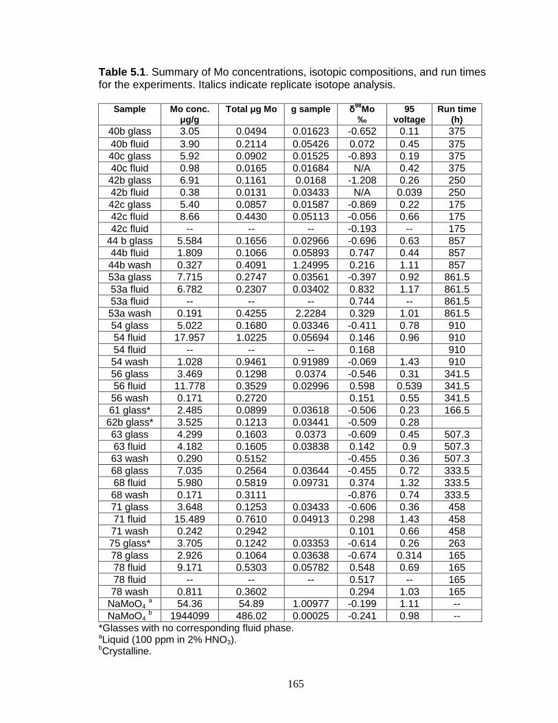
165

Table 5.1 . Summary of Mo concentrations, isotopic compositions, and run times for the experiments. Italics indicate replicate isotope analysis.

Sample Mo conc.

µg/g Total µg Mo g sample δ

98Mo ‰

95 voltage

Run time (h)

40b glass 3.05 0.0494 0.01623 -0.652 0.11 375 40b fluid 3.90 0.2114 0.05426 0.072 0.45 375 40c glass 5.92 0.0902 0.01525 -0.893 0.19 375 40c fluid 0.98 0.0165 0.01684 N/A 0.42 375 42b glass 6.91 0.1161 0.0168 -1.208 0.26 250 42b fluid 0.38 0.0131 0.03433 N/A 0.039 250 42c glass 5.40 0.0857 0.01587 -0.869 0.22 175 42c fluid 8.66 0.4430 0.05113 -0.056 0.66 175 42c fluid -- -- -- -0.193 -- 175

44 b glass 5.584 0.1656 0.02966 -0.696 0.63 857 44b fluid 1.809 0.1066 0.05893 0.747 0.44 857 44b wash 0.327 0.4091 1.24995 0.216 1.11 857 53a glass 7.715 0.2747 0.03561 -0.397 0.92 861.5 53a fluid 6.782 0.2307 0.03402 0.832 1.17 861.5 53a fluid -- -- -- 0.744 -- 861.5 53a wash 0.191 0.4255 2.2284 0.329 1.01 861.5 54 glass 5.022 0.1680 0.03346 -0.411 0.78 910 54 fluid 17.957 1.0225 0.05694 0.146 0.96 910 54 fluid -- -- -- 0.168 910 54 wash 1.028 0.9461 0.91989 -0.069 1.43 910 56 glass 3.469 0.1298 0.0374 -0.546 0.31 341.5 56 fluid 11.778 0.3529 0.02996 0.598 0.539 341.5 56 wash 0.171 0.2720 0.151 0.55 341.5 61 glass* 2.485 0.0899 0.03618 -0.506 0.23 166.5 62b glass* 3.525 0.1213 0.03441 -0.509 0.28 63 glass 4.299 0.1603 0.0373 -0.609 0.45 507.3 63 fluid 4.182 0.1605 0.03838 0.142 0.9 507.3 63 wash 0.290 0.5152 -0.455 0.36 507.3 68 glass 7.035 0.2564 0.03644 -0.455 0.72 333.5 68 fluid 5.980 0.5819 0.09731 0.374 1.32 333.5 68 wash 0.171 0.3111 -0.876 0.74 333.5 71 glass 3.648 0.1253 0.03433 -0.606 0.36 458 71 fluid 15.489 0.7610 0.04913 0.298 1.43 458 71 wash 0.242 0.2942 0.101 0.66 458 75 glass* 3.705 0.1242 0.03353 -0.614 0.26 263 78 glass 2.926 0.1064 0.03638 -0.674 0.314 165 78 fluid 9.171 0.5303 0.05782 0.548 0.69 165 78 fluid -- -- -- 0.517 -- 165 78 wash 0.811 0.3602 0.294 1.03 165

NaMoO4 a 54.36 54.89 1.00977 -0.199 1.11 --

NaMoO4 b 1944099 486.02 0.00025 -0.241 0.98 --

*Glasses with no corresponding fluid phase. aLiquid (100 ppm in 2% HNO3). bCrystalline.

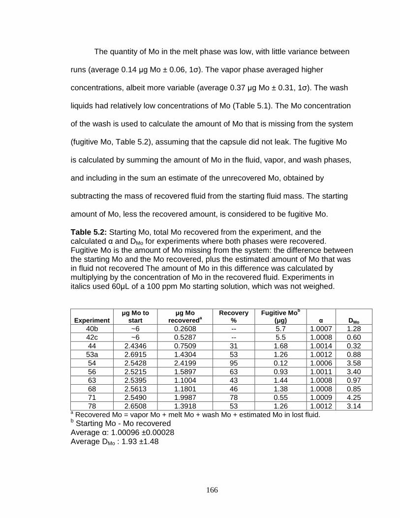
166

The quantity of Mo in the melt phase was low, with little variance between

runs (average 0.14 µg Mo ± 0.06, 1σ). The vapor phase averaged higher

concentrations, albeit more variable (average 0.37 µg Mo ± 0.31, 1σ). The wash

liquids had relatively low concentrations of Mo (Table 5.1). The Mo concentration

of the wash is used to calculate the amount of Mo that is missing from the system

(fugitive Mo, Table 5.2), assuming that the capsule did not leak. The fugitive Mo

is calculated by summing the amount of Mo in the fluid, vapor, and wash phases,

and including in the sum an estimate of the unrecovered Mo, obtained by

subtracting the mass of recovered fluid from the starting fluid mass. The starting

amount of Mo, less the recovered amount, is considered to be fugitive Mo.

Table 5.2: Starting Mo, total Mo recovered from the experiment, and the calculated α and DMo for experiments where both phases were recovered. Fugitive Mo is the amount of Mo missing from the system: the difference between the starting Mo and the Mo recovered, plus the estimated amount of Mo that was in fluid not recovered The amount of Mo in this difference was calculated by multiplying by the concentration of Mo in the recovered fluid. Experiments in italics used 60µL of a 100 ppm Mo starting solution, which was not weighed.

Experiment µg Mo to

start µg Mo

recovered a Recovery

% Fugitive Mo b

(µg) α DMo 40b ~6 0.2608 -- 5.7 1.0007 1.28 42c ~6 0.5287 -- 5.5 1.0008 0.60 44 2.4346 0.7509 31 1.68 1.0014 0.32 53a 2.6915 1.4304 53 1.26 1.0012 0.88 54 2.5428 2.4199 95 0.12 1.0006 3.58 56 2.5215 1.5897 63 0.93 1.0011 3.40 63 2.5395 1.1004 43 1.44 1.0008 0.97 68 2.5613 1.1801 46 1.38 1.0008 0.85 71 2.5490 1.9987 78 0.55 1.0009 4.25 78 2.6508 1.3918 53 1.26 1.0012 3.14

a Recovered Mo = vapor Mo + melt Mo + wash Mo + estimated Mo in lost fluid. b Starting Mo - Mo recovered Average α: 1.00096 ±0.00028 Average DMo : 1.93 ±1.48

167

Calculation of α (vapor-melt) and DMo (vapor-melt)

The fractionation factor, α, for Mo isotopes between vapor and melt can be

calculated from the δ98Mo values of these phases for each experiment where

both were recovered (Fig. 5.3):

(5.1) (1000 + δ98Movapor)/(1000 + δ98Momelt) = α

The average α for all the experiments is 1.00096 (0.96‰), ± 0.00028 (0.28‰,

1σ). Likewise, where both run products were recovered, DMo, the elemental

partition coefficient between the vapor and melt, can be calculated from the

concentration of Mo in these phases (Fig. 5.3). The average DMo for the ten

paired products is 1.93 ±1.48, which is similar to previous studies (Candela and

Holland, 1984). In calculating α and DMo, the Mo in the wash is not included,

because there is uncertainty as to whether the Mo in the wash belongs to the

fluid phase or to the melt phase.

Discussion

Possible problems

It is important to identify the potential pitfalls of the experimental setup and

recovery procedure, as these might significantly affect the results. The first

problem is that for most of the experiments, the efficiency of recovery of Mo from

the total system (vapor + melt + wash) was generally less than 50% (Table 5.1).

This implies that some to most of the initial Mo with which the system began was

lost (fugitive Mo). One possibility is that the Au capsule adsorbed some of this

168

fugitive Mo. This effect, if present, was not related to run length (Fig. 5.4). If Mo

uptake into a third phase involves a different isotopic fractionation of Mo, then it

might be apparent in the α value (Fig. 5.4). There appears to be a small effect of

Mo loss on the overall fractionation between the two phases. The R2 of the trend

between these two factors is 0.6, but it is a very shallow trend. It suggests that

experiments with the least fugitive Mo might be more reflective of the true

isotopic fractionation between vapor and melt. Small fragments of several Au run

capsules have been dissolved in order to determine whether a significant

quantity of Mo entered the capsule.

Partitioning of Mo between the melt and fluid might be dependent on the

concentration of Mo in the system. Natural systems are likely to have much lower

concentrations of Mo (1-2 µg/g). The blue color of the glass

beads suggest the possibility that Mo in the glass is polymerized, and Mo

polymers are likely to be more stable at high Mo concentrations. However,

the similarity of the DMo value obtained here to previous results suggests that this

may not be a primary concern.

169

Figure 5.1: δ98Mo of run products versus run time. Orange circles are melt, blue circles are vapor. The starred experiment (54) did not have an isobaric quench. Grey tie lines connect run products from the same experiment.

There is the possibility that inclusions of vapor were trapped in the melt

upon quench. Data suggest that such inclusions contribute Mo that is less than

5% of the total present in the melt. A simple calculation shows that a 5%

contribution from the vapor to the melt composition is not significant enough to

shift its isotopic composition. Assuming that the vapor has an average δ98Mo of

0.4‰, the isotopic composition of the melt would shift by only +0.02‰ for a 5%

contribution of vapor. This is well within the external reproducibility of δ98Mo

measurements, and, thus, is not a significant source of error to the δ98Mo values

for the melt phase.

170

Interpretation of experimental results

The most important observation is that the average δ98Mo values for the

run products are isotopically distinct from the starting Mo composition. This is

strong evidence that fractionation between the two phases has taken place. The

vapor phase is consistently isotopically heavier than the coexisting melt, which

was expected based on equilibrium fractionation theory.

No trend in δ98Mo is apparent, in either phase, with run length. This time-

independence suggests that the system has quickly reached equilibrium with

respect to Mo isotopes (Fig. 5.1). At 320°C and 10 M Pa, 6 days were required to

reach equilibrium with respect to Mo solubility according to Rempel et al. (2006).

Therefore, it is likely that the time to reach isotopic equilibrium is shorter than the

shortest experiment, ~7 days. With respect to Mo concentration of the run

products, again, no trend was apparent with run length (Fig. 5.2), which supports

the assertion that the system reached equilibrium in less than 7 days.

Molybdenum concentration and δ98Mo are only poorly correlated for either phase

(Fig. 5.5), but the amount of Mo captured in the glass shows more consistency.

This could be related to incomplete collection of the vapor run product at the end

of the experiment.

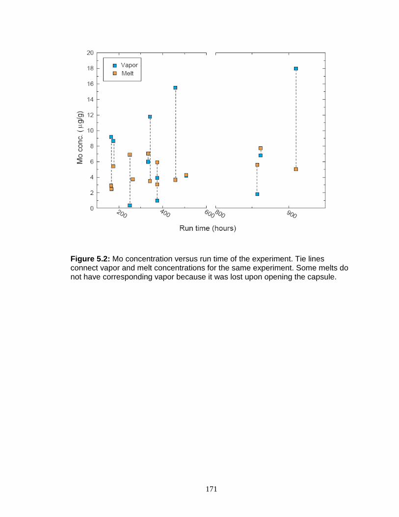
171

Figure 5.2: Mo concentration versus run time of the experiment. Tie lines connect vapor and melt concentrations for the same experiment. Some melts do not have corresponding vapor because it was lost upon opening the capsule.

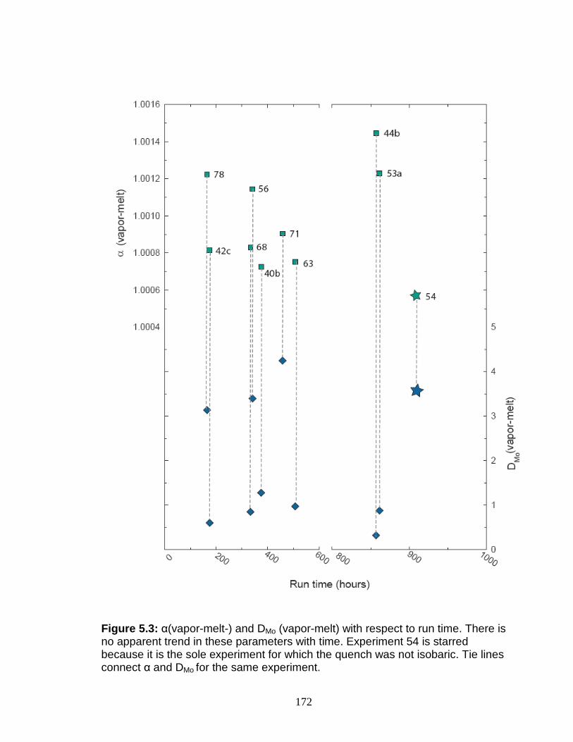
172

Figure 5.3: α(vapor-melt-) and DMo (vapor-melt) with respect to run time. There is no apparent trend in these parameters with time. Experiment 54 is starred because it is the sole experiment for which the quench was not isobaric. Tie lines connect α and DMo for the same experiment.

173

Figure 5.4: (Top ): Fugitive Mo (µg) versus run time. (Bottom): Fugitive Mo (µg) as a function of α value. There appears to be a shallow trend towards more fractionation with increasing quantities of fugitive Mo.

174

Figure 5.5: Molybdenum isotopic composition as a function of Mo concentration. The δ98Mo of the starting material is shown at the right. 100µl (containing 25 µg/g Mo) of the material was placed in the capsule at the start.

175

When discussing possible causes for the observed fractionation between

the melt and the vapor, we assume that the fractionation is an equilibrium isotope

effect. Equilibrium stable isotope fractionation is a function of the vibrational

energies of molecules containing atoms of different masses (Urey, 1947). For

heavier elements with smaller overall fractionations, the most important

processes governing stable isotope partitioning include oxidation state,

coordination number, electron configuration, and bonding environment (e.g., to

H, O or N), among others (Schauble, 2004). A phase with high bond strength and

bond stiffness will tend to favor the heavier isotopes of an element. Thus, a

phase with high oxidation state, low coordination number, or low-spin electron

configuration compared to the phase with which it is in equilibrium, should be

isotopically heavier.

In the system experimentally examined here, vapor phase Mo is (VI) in a

trigonal planar coordination (Rempel et al., 2006; 2009), while in the melt it is (VI)

with tetrahedral and octahedral coordination (Farges et al., 2006). Thus, heavier

δ98Mo values in the vapor phase may be a result of a coordination number

change around Mo as it moves into the melt phase.

It is, however, possible that the oxidation state of Mo is different in the

melt and vapor phases. One reason to suspect that this might be the case is the

blue color of the quenched melt. The blue color might be indicative of

polyoxometalate complexes or Mo polymers, in which Mo has been partially or

wholly reduced from (VI) to (V) or (IV). In this case, fractionation theory predicts

that the heavy isotopes will remain with the higher oxidation state. If the Mo in the

176

melt is reduced, its isotopic composition would become lighter, while the vapor

became isotopically heavier. Based on the data, it does not seem possible to

differentiate between these two candidates. If any of the Mo is (V), another

problem presents itself. This is the possibility that the Mo(V) would not reach

equilibrium with the double spike, or might not be captured efficiently by the

existing column chemistry. The second instance could significantly fractionate Mo

isotopes, which, if the first instance were true, could not be corrected by the

double-spike process. Incomplete recovery of Mo(V) from the column chemistry

could also be a reason that the Mo mass balance failed.

Geological implications We have shown that there is well-resolved Mo isotopic fractionation in an

experimental vapor-melt system that mimics how Mo may become enriched in a

volatile phase in a magmatic-hydrothermal system. One major implication of this

is that it suggests that separation of isotopically heavy Mo into a volatile phase

should generate an isotopically lighter reservoir of Mo in the crust (relative to the

starting Mo composition). Such an interpretation is probably generally applicable

to oxidized systems. However, the presence of sulfur and other volatiles is likely

to change the coordination environment and oxidation state of Mo (Farges et al.,

2006). This would affect the Mo fractionation factor to an unknown degree,

because of differences in the bond partners to Mo in each phase. It is still

unknown what the fractionation associated with molybdenite formation is.

Molybdenite may crystallize from the vapor phase as temperature falls, and

hydrated MoO3 reacts with H2S. Hannah et al. (2007) suggested that

177

crystallization of molybdenite can be described as a Rayleigh distillation process.

If the starting vapor Mo is isotopically heavy, then by Rayleigh fractionation,

MoS2 should evolve to even heavier values. While on balance the measured

MoS2 δ98Mo values have been heavy, some light δ98Mo values have also been

reported. This could mean that the fraction of Mo removed from the vapor during

distillation was small. The main problem with applying the experimental data is

that, while the starting δ98Mo of the Mo in the experimental system was known,

this is rarely the case in a natural system. Nevertheless, these experiments

provide the first estimate for the high temperature/high-pressure equilibrium

isotope fractionation of Mo between a vapor phase and a melt phase.

178

Conclusions In this work, a number of directions have been explored with respect to Mo

isotopes, and suggest areas where further research could significantly strengthen

the current understanding of the global Mo isotope system. Progress towards a

more quantitative model of the cycling of Mo would improve the ability to use Mo

isotopes as proxies of redox conditions.

The behavior of Mo in a seasonally anoxic estuary over the past century

was studied. In the Chesapeake Bay, annual changes in nutrient runoff influence

the intensity of O2 depletion in the deep water. Molybdenum is enriched in

Chesapeake Bay sediments, and appears to be lost from the water column.

Estuaries are the interface between rivers and the ocean, and as such process

weathered material arriving from the interiors of continents. This particular

avenue would benefit from a more complete understanding of the processing of

Mo in the watershed. Since most rivers that have been investigated (Archer and

Vance, 2008), including the Susquehanna River in this dissertation, have Mo

isotope values that are heavy, understanding the chemical or physical

weathering processes that might impart this signature is very important. These

heavy values might be purely indicative of the source material of Mo in the

watershed, in which case study of the actual rocks and sediments in the drained

basin would be important. This could then be used to determine the seasonal

variation in degree and rate of processing that takes place during transport

downstream.

179

The study of Mediterranean sediments illustrates the need to better

understand Mo isotope behavior in the so-called suboxic regimes. In the

literature, 'suboxic' has been used as a catch-all for most Mo isotope signatures

that are not distinctly anoxic/euxinic, or derived from MnOx adsorption. A wide

range of values occur in low-O2 settings, and it should be possible to distinguish

processes that are imparting these isotope signatures. Sequential extraction of

Mo from different sedimentary components might show that the array of

signature is related to a mix of values derived from adsorption to FeOx, pyrite,

organic matter, or from conversion to partial-thiomolybdate species. Additionally,

a better understanding of the diagenetic behavior of Mo isotopes in sediments

and in pore water would be useful in differentiating between primary isotope

signatures and those reset by diagenetic processing. More holistic studies of

modern systems, that include sediments, porewater, trapped particles, and

overlying water (e.g., Dahl et al., 2009), would contribute to a more complete

modeling of Mo isotope cycling.

In the final chapter, we experimentally determined a Mo isotope

fractionation factor between vapor and melt. The history of experimentally

determining isotope fractionation factors is long (e.g., Urey, 1947; McCrea, 1950)

and has led to the ubiquitous use of oxygen isotopes in paleoceanography, and

in metamorphic systems. These factors are fundamental to understanding the

measured isotope ratios in sediments, ore deposits, or other rocks. Thus, an

important future direction is to expand the database of Mo isotope fractionation

180

factors, which should lead to the increased ability to understand the

measurements made in natural systems.

181

Appendices

Appendix 1. Supplemental information to Chapter 3. The northernmost samples are from a 1979 core in the Conowingo Dam

reservoir on the Susquehanna River, the main tributary to the Chesapeake Bay

(Helz et al., 1985). The Susquehanna River provides about half the total fresh

water to the Bay, and dominates the sediment budget (Hobbs et al., 1992).

One sample from each of three separate cores (BH N, M, and H) taken in

Baltimore Harbor were analyzed. Industrial activity in the Baltimore area has left

the harbor sediments contaminated with Cu, Zn, and other metals. The Harbor is

frequently dredged, disturbing any age-depth relationship (Mason et al., 2004;

Sinex and Helz, 1982). Contamination is greatest in the inner harbor (Cores N

and M), and eases eastward towards the Bay's main stem (Core H). For

example, Cu concentrations are: 730 µg/g Cu in Core N, 1800 µg/g in Core M,

and 500 µg/g in Core H (Dolor et al., 2009; Sinex and Helz, 1982).

Surface samples were obtained from a shallow to deep water traverse,

close to the location of cores RD and 55. Increased Mn content in shallow-water

sediments, compared to deep-water sediments, is the result of a process called

refluxing. In this process, MnOx that has fallen out in deeper water as particles is

dissolved when reducing conditions develop in summer (Helz et al., 1985). These

surface samples (Depth Traverse, DT, 0902, 0903, and 0907) are characterized

by high Mn concentrations that decrease with increasing water depth. DT 0902,

at 3.4m water depth, has 3000 µg/g Mn, DT 0903 at 6.7 m has 2200 µg/g, and

182

DT 0907 at 26.2 m has 1000 µg/g Mn (Dolor et al., 2009). Only the fine fraction of

these sediment samples (<63 µm) was available.

Core PC-6 is our most southerly sample site. It samples sediments

approximately 30 km south of Core 55. The samples come from below the

horizon that represents the regional introduction of European agriculture (~1700

ybp), as determined by ragweed pollen abundance (Helz et al., 2000). The ages

of these three samples are approximately 1300, 800, and 300 ybp, interpolated

from a sedimentation rate of 0.11 cm/yr (Helz et al., 2000).

In the vicinity of PC-6, shoreline bluffs of the Miocene-aged Fairhaven

member of the Calvert Formation stand above the Chesapeake Bay. The

Fairhaven member is characterized by enrichments in several redox-sensitive

metals, including Mo. The Fairhaven was digested five separate times and each

digestion was analyzed several times. These data are presented in table A1.

Organic carbon content in weight percent (TOC) was measured on carbonate-

free samples for the two cores, RD and 55. These data are presented in table

A2.

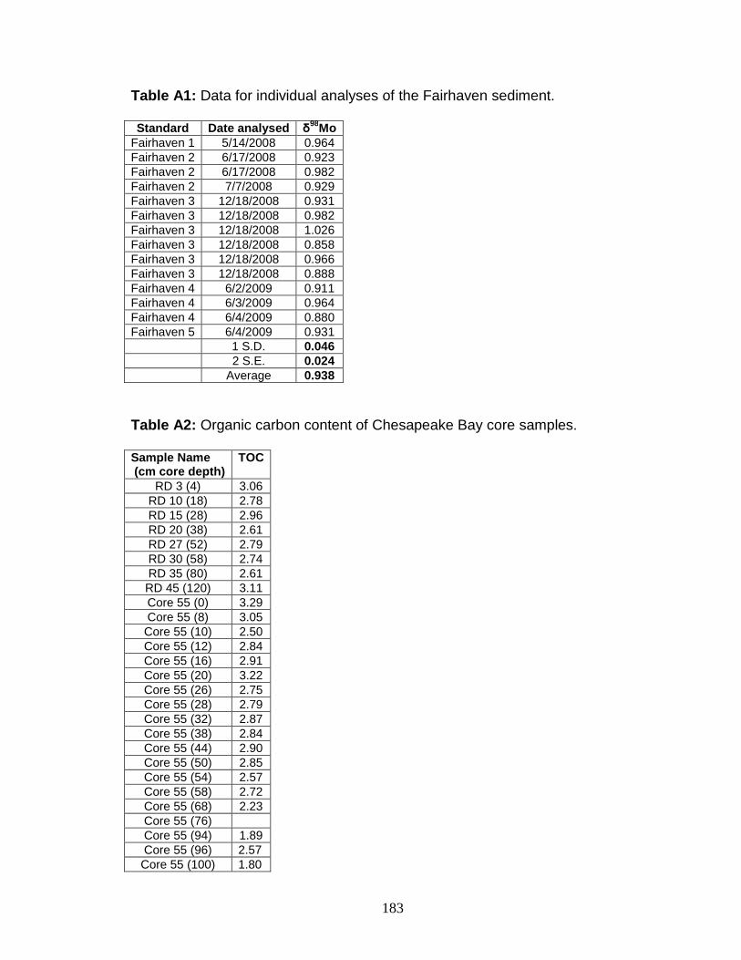
183

Table A1: Data for individual analyses of the Fairhaven sediment.

Standard Date analysed δ98Mo

Fairhaven 1 5/14/2008 0.964 Fairhaven 2 6/17/2008 0.923 Fairhaven 2 6/17/2008 0.982 Fairhaven 2 7/7/2008 0.929 Fairhaven 3 12/18/2008 0.931 Fairhaven 3 12/18/2008 0.982 Fairhaven 3 12/18/2008 1.026 Fairhaven 3 12/18/2008 0.858 Fairhaven 3 12/18/2008 0.966 Fairhaven 3 12/18/2008 0.888 Fairhaven 4 6/2/2009 0.911 Fairhaven 4 6/3/2009 0.964 Fairhaven 4 6/4/2009 0.880 Fairhaven 5 6/4/2009 0.931

1 S.D. 0.046 2 S.E. 0.024 Average 0.938

Table A2: Organic carbon content of Chesapeake Bay core samples.

Sample Name (cm core depth)

TOC

RD 3 (4) 3.06 RD 10 (18) 2.78 RD 15 (28) 2.96 RD 20 (38) 2.61 RD 27 (52) 2.79 RD 30 (58) 2.74 RD 35 (80) 2.61 RD 45 (120) 3.11 Core 55 (0) 3.29 Core 55 (8) 3.05 Core 55 (10) 2.50 Core 55 (12) 2.84 Core 55 (16) 2.91 Core 55 (20) 3.22 Core 55 (26) 2.75 Core 55 (28) 2.79 Core 55 (32) 2.87 Core 55 (38) 2.84 Core 55 (44) 2.90 Core 55 (50) 2.85 Core 55 (54) 2.57 Core 55 (58) 2.72 Core 55 (68) 2.23 Core 55 (76) Core 55 (94) 1.89 Core 55 (96) 2.57 Core 55 (100) 1.80

184

Appendix 2. Supplemental information to Chapter 4

Core photos

On board ship, each core is cut in half, sectioned, and photographed. The

photographs are archived in an online database that is available to researchers

and the public at http://iodp.tamu.edu/janusweb/imaging/photo.shtml. Core

photographs for Leg 160, Site 969, hole D, cores 4H (Fig. A1) and 5H (Fig. A2),

which were used in this study, are reproduced here with the permission of the

International Ocean Drilling Program. To identify the specific location of a sample

on these photos, identify the section number of interest along the top margin.

Then, locate the cm core depth along the left hand margin.

185

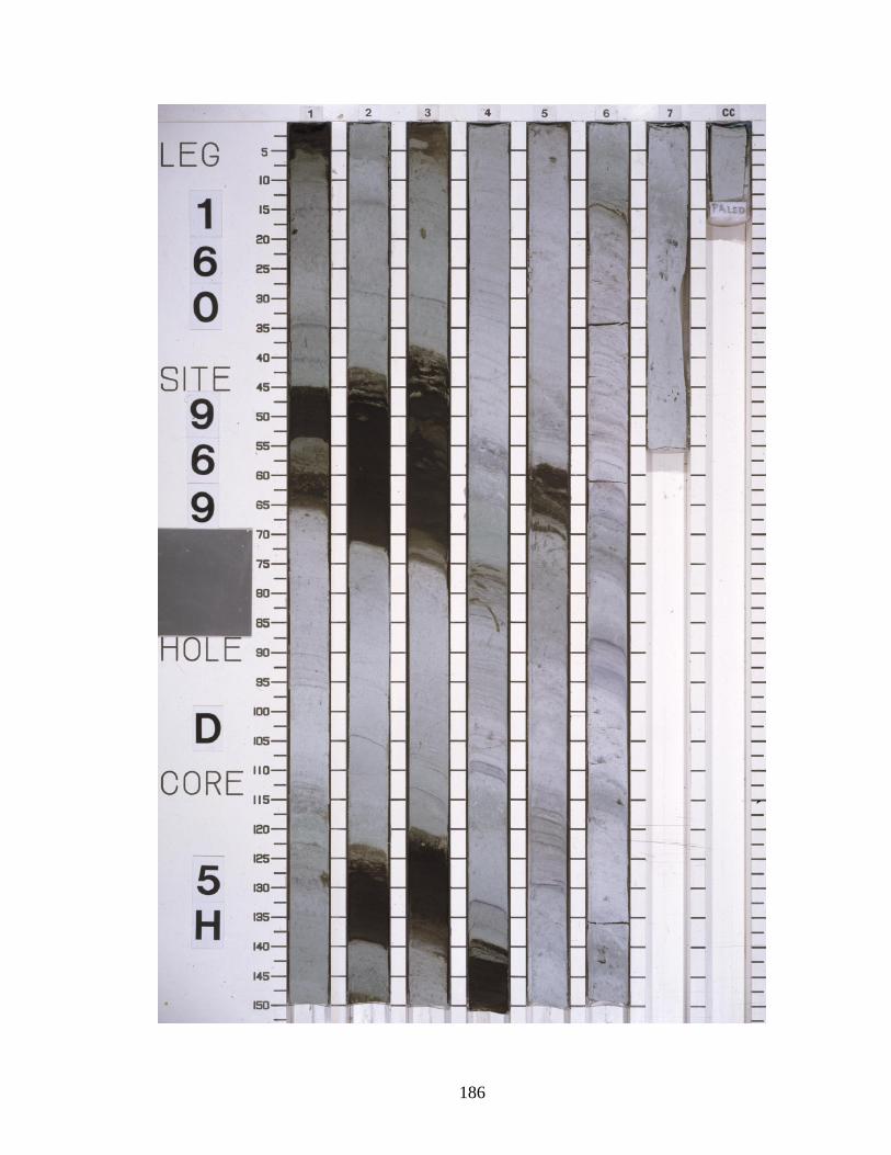
186

187

Duplicate Samples

Table A3: Molybdenum isotope data for samples that were processed twice. In some cases more than one measurement was made of the sample solution. Duplicate samples δ

98Mo 4H-2, 131 (A) 1.317 a 4H-2, 131 (B) 1.237 4H-2, 61 (A) 0.919 4H-2, 61 (B) 0.966 5H-1, 50 (A) 0.579 5H-1, 50 (B) 0.516 5H-3, 100 (A) 2.369 5H-3, 100 (B) 2.519 b

a 4H-2, 131(A) was measured 4 times, averaging 1.317±0.03. b Average of two measurements (2.556, 2.481)

Sample preparation for sulfur isotope analysis

A small subset of the Mediterranean samples (both sapropels and

hemipelagic) was processed for multiple sulfur isotope analysis. Sediment

powders were first boiled in 5M HCl to release acid volatile sulfur (AVS), then

treated with a hot chrome(II)-reduction solution to reduce pyrite (Canfield et al.,

1986). No AVS was produced in any of the samples. The H2S evolved in each

CRS reaction was captured as Ag2S in a solution of 10% AgNO3. Ag2S was

cleaned with 250 mL of Milli Q water and 50 mL of 1 M NH4OH and dried. For

fluorinations, samples were reacted in Ni bombs with F2 gas at ~250 ºC for ~8

hours. This quantitatively converts the Ag2S to SF6. Product SF6 was then

purified with several liquid N2 distillations, and by gas chromatography on a 12’

molecular sieve 5 Å/Haysep Q column with a thermal conductivity detector. The

S isotopic abundances of the purified SF6 was analyzed on a Finnigan MAT 253

dual inlet mass spectrometer at m/e- values of 127, 128, 129, and 131 (32SF5+,

33SF5+, 34SF5

+, and 36SF5+). Analytical uncertainties on S isotope measurements,

188

estimated from long-term reproducibility of Ag2S fluorinations, are 0.14, 0.008,

and 0.20 (1σ) for δ34S, ∆33S, and ∆36S, respectively (e.g., Zerkle et al., 2008).

The minor isotope compositions of sulfur species are presented using the

∆3XS notation, which describes the deviation of a sample datum in 33S or 36S (in

‰) from a reference fractionation line:

( )[ ]1/515.0

234343333 −−=∆ SiHsample RRSS δ

and

( )[ ]1/90.1

234343636 −−=∆ SiHsample RRSS δ

The exponents 0.515 and 1.90 are reference values assigned to approximate

mass-dependent fractionations during thermodynamic equilibrium isotope

exchange at low temperature (Hulston and Thode, 1965; Farquhar et al., 2003;

Farquhar and Wing, 2003; Johnston et al., 2007; Ono et al., 2007). Small

deviations from these reference values occur in biogeochemical systems

because the redistribution of mass between sulfur pools by, e.g., mixing or

Rayleigh processes, results in the isotope ratios of sulfur pools evolving in a

linear fashion, which differs from the exponential relationship calculated for

reference fractionation arrays. For a more detailed explanation of how these

signatures are produced in natural systems, see Farquhar et al. (2003, 2007) and

Johnston et al. (2005, 2007).

Mass balance calculations

The primary source of fresh water to the Mediterranean Sea is the Nile

River. It contributes ~5 x 1014 L/y of water, with an average Mo concentration of

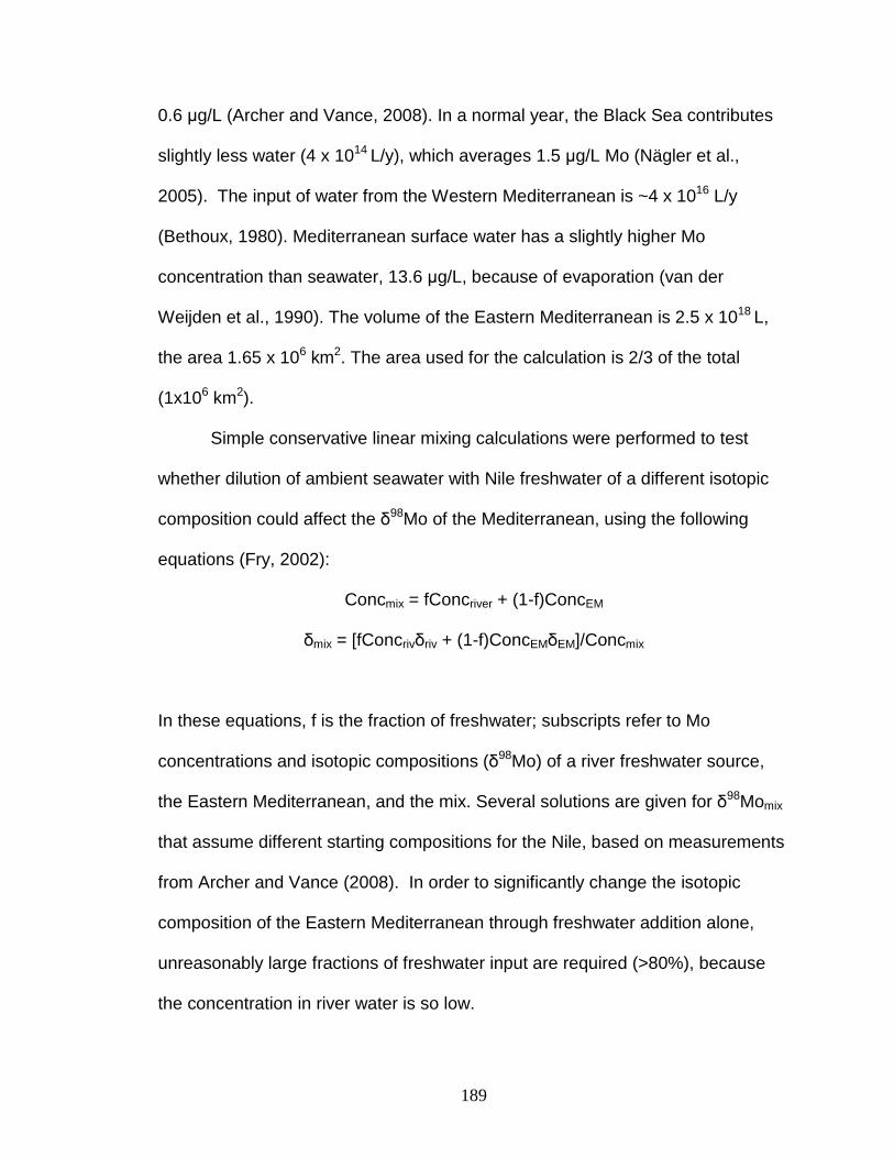
189

0.6 µg/L (Archer and Vance, 2008). In a normal year, the Black Sea contributes

slightly less water (4 x 1014 L/y), which averages 1.5 µg/L Mo (Nägler et al.,

2005). The input of water from the Western Mediterranean is ~4 x 1016 L/y

(Bethoux, 1980). Mediterranean surface water has a slightly higher Mo

concentration than seawater, 13.6 µg/L, because of evaporation (van der

Weijden et al., 1990). The volume of the Eastern Mediterranean is 2.5 x 1018 L,

the area 1.65 x 106 km2. The area used for the calculation is 2/3 of the total

(1x106 km2).

Simple conservative linear mixing calculations were performed to test

whether dilution of ambient seawater with Nile freshwater of a different isotopic

composition could affect the δ98Mo of the Mediterranean, using the following

equations (Fry, 2002):

Concmix = fConcriver + (1-f)ConcEM

δmix = [fConcrivδriv + (1-f)ConcEMδEM]/Concmix

In these equations, f is the fraction of freshwater; subscripts refer to Mo

concentrations and isotopic compositions (δ98Mo) of a river freshwater source,

the Eastern Mediterranean, and the mix. Several solutions are given for δ98Momix

that assume different starting compositions for the Nile, based on measurements

from Archer and Vance (2008). In order to significantly change the isotopic

composition of the Eastern Mediterranean through freshwater addition alone,

unreasonably large fractions of freshwater input are required (>80%), because

the concentration in river water is so low.

190

Figure A3: Isotope mixing model for the Eastern Mediterranean with Nile fresh water. The upper three mixes all assume a starting δ98Mo of modern seawater. Mix 4 changes the starting δ98Mo to 1.8‰. The parameters that change are the Mo concentration of Nile water, and the δ98Mo (Archer and Vance, 2008). Mix 1 has (1.4 µg/L, 0.2‰), mix 2 has (1.4 µg/L, 0.4‰), mix 3 has (0.5 µg/L, 1.2‰), mix 4 has (1.4 µg/L, 0.2‰).

Some major element ratios can be useful when attempting to identify a

source location for the elements (e.g., Nijenhuis et al., 1998). One major source

of dust to the Mediterranean is the Sahara desert, and one sample of North

Saharan Dust, collected in Cairo (Linke et al., 2006), does appear to have an

elemental composition very similar to the Mediterranean sapropels. However,

Nile particulate matter (Krom et al., 1999), which could potentially reach Site 969,

is not compositionally similar (Fig. A.4). The problem with dust as a source of

191

trace elements is two-fold: 1.) sapropel deposition took place during wetter

periods, when dust transport and deposition would be reduced (Wehausen and

Brumsack, 1998), and 2.) calculations suggest that the trace element budget in

dust is not high enough to supply sapropels with the requisite quantities (e.g.,

Nijenhuis et al., 1998). Based on these calculations, we suggest that seawater

was indeed the source of Mo, V, and Re to the sediments. In order to avoid a

drawdown scenario, seawater was probably circulating between the Eastern and

Western Mediterranean.

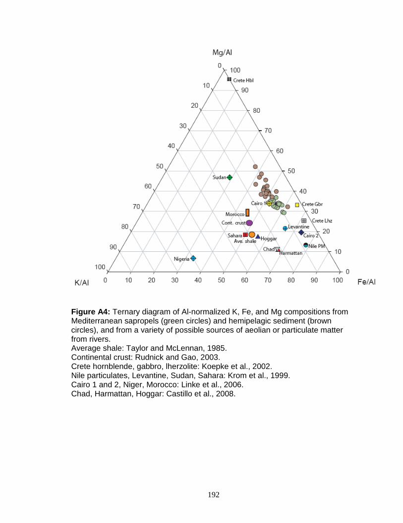
192

Figure A4: Ternary diagram of Al-normalized K, Fe, and Mg compositions from Mediterranean sapropels (green circles) and hemipelagic sediment (brown circles), and from a variety of possible sources of aeolian or particulate matter from rivers. Average shale: Taylor and McLennan, 1985. Continental crust: Rudnick and Gao, 2003. Crete hornblende, gabbro, lherzolite: Koepke et al., 2002. Nile particulates, Levantine, Sudan, Sahara: Krom et al., 1999. Cairo 1 and 2, Niger, Morocco: Linke et al., 2006. Chad, Harmattan, Hoggar: Castillo et al., 2008.

193

Bibliography

Adelson, J.M., Helz, G.R., Miller, C.V., 2001. Reconstructing the rise of recent coastal anoxia: Molybdenum in Chesapeake Bay sediments. Geochim. Cosmochim. Acta. 65, 237-252. Albarede, F., Beard, B.L., 2004. Analytical methods for non-traditional stable isotopes. In: Johnson, C.M., Beard, B.L., Albarede, F., (Eds.) Geochemistry of non-traditional stable isotopes. Rev. Mineral. Geochem. 55, 113-152. Albarède, F., Telouk, P., Blichert-Toft, J., Boyet, M., Agranier, A., Nelson, B., 2004. Precise and accurate isotopic measurements using multiple-collector ICPMS. Geochim. Cosmochim. Acta. 68, 2725-2744. Algeo, T.J, 2004. Can marine anoxic events draw down the trace element inventory of seawater? Geology. 32, 1057-1060. Algeo, T.J., Lyons, T., W., 2006. Mo-TOC covariation in modern anoxic marine environments: Implications for analysis of paleoredox and paleohydrographic conditions. Paleoceanograpy. 12, PA1016, doi:10.1029/2004PA001112. Algeo, T.J., Lyons, T.W.,. Blakey, R.C., Over, D.J., 2007. Hydrographic conditions of the Devono-Carboniferous North American Seaway inferred from sedimentary Mo-TOC relationships, Palaeogeogr. Palaeoclimatol. Palaeoecol. 256, 204–230. Anbar A.D., Creaser, R.A., Papanastassiou, D.A., Wasserburg, G.J., 1992. Rhenium in seawater: confirmation of generally conservative behavior. Geochim. Cosmochim. Acta 56, 4099-4104. Anbar, A.D., Knab, K.A., Barling, J., 2001. Precise determination of mass-dependent variations in the isotopic composition of molybdenum using MC-ICPMS. Anal. Chem. 73, 1425-1431.

Archer, C., Vance, D., 2008. The isotopic signature of the global riverine molybdenum flux and anoxia in the ancient oceans. Nature Geosci. 1, 597-600.

Arnold, G.A., Anbar, A.D., Barling, J., Lyons, T.W., 2004. Molybdenum isotope evidence for widespread anoxia in Mid-Proterozoic oceans. Science. 304, 87-90. Barling, J., Anbar, A.D., 2004. Molybdenum isotope fractionation during adsorption by manganese oxides. Earth Planet. Sci. Lett. 217, 315-329. Barling, J., Arnold, G.L., Anbar, A.D., 2001. Natural mass-dependent variations in the isotopic composition of molybdenum. Earth Planet Sci. Lett. 193, 447-457.

194

Belshaw, N.S., Freedman, P.A., O'Nions, R.K., Frank, M., Guo, Y., 1998. A new variable dispersion double-focusing plasma mass spectrometer with performance illustrated for Pb isotopes. Int. J. Mass Spectrom. 181, 51-58. Bermin, J., Vance, D., Archer, C., Statham, P.J., 2006. The determination of the isotopic composition of Cu and Zn in sea water. Chem. Geol. 226, 280-297. Bertine, K.K., Turekian, K.K., 1973. Molybdenum in marine sediments, Geochim. Cosmochim. Acta. 37, 1415–1434. Béthoux, J.P., 1980. Mean water fluxes across sections in the Mediterranean Sea evidenced on the basis of water and salt budget and of observed salinities. Oceanol. Acta. 9, 79–88. Biggs, R.B., 1970. Sources and distribution of suspended sediment in northern Chesapeake Bay. Mar. Geol. 9, 187-201. Boothman, W.S., Coiro, L.L., 2009. Laboratory determination of molybdenum accumulation rates as a measure of hypoxic conditions. Estuaries and Coasts. 32, 642-653. Bostick, B.C., Fendorf, S., Helz, G.R., 2003. Differential adsorption of molybdate and tetrathiomolybdate on pyrite (FeS2), Environ. Sci. Technol. 37, 285-291, 2003. Böttcher, M. E., Rinna, J., Warning, B., Wehausen, R., Howell, M. W., Schnetger, B., Stein, R., Brumsack, H. -J., Rullkötter J., 2003. Geochemistry of sediments from the connection between the western and the eastern Mediterranean Sea (Strait of Sicily, ODP Site 963). Palaeogeog., Palaeoclim., Palaeoecol. 190, 165-194 Boyd, F.R., Mertzman, S.A., 1987. Composition and structure of the Kaapvaal lithosphere, Southern Africa, in: Mysen, B.O. (Ed.), Magmatic Processes. Geochem. Soc. Spec. Publ., 13–24. Bruland, K., 1983. Trace metals in seawater. Chem. Oceanog. 8, 157-220. Brumsack, H.-J., 1986. The inorganic geochemistry of Cretaceous black shales (DSDP Leg 41) in comparison to modern upwelling sediments from the Gulf of California. In: Shackleton, N.J., Summerhayes, C.P., (Eds): North Atlantic Paleoceanography. Geol. Soc. Spec. Publ. 21, 447–462. Brumsack, H.-J., 1989. Geochemistry of recent TOC-rich sediments from the Gulf of California and the Black Sea. Geolog. Rundschau. 78, 851-882.

195

Brunner, B., Bernasconi, S.M., 2005. A revised isotope fractionation model for dissimilatory sulfate reduction in sulfate reducing bacteria. Geochim. Cosmochim.Acta. 69, 4759–4771. Calvert, S.E., Pedersen, T.F., 1993. Geochemistry of Recent oxic and anoxic marine sediments: Implications for the geological record, Mar. Geol. 113, 67-88. Calvert, S.E., Price, N.B., 1977. Chemical variation in ferromanganese nodules and associated sediments from the Pacific Ocean, Mar. Chem. 5, 43-74. Camerlenghi, A., 1990. Anoxic basins of the Eastern Mediterranean: Geological framework. Mar. Chem. 31, 1–19. Camerlenghi A., Cita, M.B., 1987. Setting and tectonic evolution of some Eastern Mediterranean deep-sea basins. Mar.Chem. 75, 31–56. Candela, P.A., 1989. The calculation of magmatic contributions to porphyry-type ore systems: Predicting fluid inclusion chemistries. Geochemical Journal. 23, 295-305. Candela, P.A., Holland, H.D., 1984. The partitioning of copper and molybdenum between silicate melts and aqueous fluids. Geochim. Cosmochim. Acta. 48, 373-380. Candela, P.A., Piccoli, P., 2005. Magmatic processes in the development of porphyry-type ore systems, in Hedenquist, J.W., Thompson, J.F.H., Goldfarb, R.J., Richards, J.R., eds., Society of economic geologists 100th Anniversary Volume, 25-38. Canfield, D.E., 1989. Reactive iron in marine sediments, Geochim. Cosmochim. Acta. 53, 619–632. Canfield, D.E., Raiswell, R., Westrich, J.T., Reaves, C.M., and Berner, R.A., 1986. The use of chromium reduction in the analysis of reduced inorganic sulfur in sediments and shales: Chem. Geol. 54, 149-155. Casford, J.S.L., Rohling, E.J., Abu-Zeid, R.H., Fontanier, C., Jorissen, F.J., Leng, M.J., Schmiedl, G., Thomson, J., 2003. A dynamic concept for eastern Mediterranean circulation and oxygenation during sapropel formation. Paleogeog., Paleoclim., Paleoecol. 190, 103-119. Castillo, S., Moreno, T., Querol, X., Alastuey, A., Cuevas, E., Herrmann, L., Mounkaila, M., Gibbons W., 2008. Trace element variation in size-fractionated African desert dusts. J. Arid Envir. 72, 1034-1045.

196

Collier, R.W., 1985. Molybdenum in the Northeast Pacific Ocean. Limnol. Oceanogr. 30, 1351-1354. Colodner, D., Sachs, J., Ravizza, G., Turekian, K., Edmond, J., Boyle, E., 1993. The geochemical cycle of rhenium: a reconnaissance. Earth Planet. Sci. Lett. 117, 205-221. Colodner, D., Edmond J., Boyle, E., 1995. Rhenium in the Black Sea: comparison with molybdenum and uranium. Earth Planet. Sci. Lett. 131, 1–15. Compston, W., Oversby, V.M., 1969. Lead isotopic analysis using a double-spike. J. Geophys. Res. 74, 4338-4348. Coplen, T.B., Böhlke, J.K., De Bievre, P., Ding, T., Holden, N.E., Hopple, J.A., Krouse, H.R., Lamberty, A., Peiser, H.S., Revesz, K., Rieder, S.E., Rosman, K.J.R., Roth, E., Taylor, P.D.P, Vocke Jr., R.D., Xiao, Y.K., 2002. Isotope-abundance variations of selected elements (IUPAC Technical Report, and references therein). Pure Applied Chem. 74, 1987 - 2017. Cooper, S.R., Brush, G.C., 1993. A 2,500-Year history of anoxia and eutrophication in Chesapeake Bay. Estuaries. 16, 617-626. Cramp, A., O'Sullivan, G.O., 1999. Neogene sapropels in the Mediterranean: a review. Mar. Geol. 153, 11-28. Cronan, D.S., 1976. Basal metalliferous sediments from the eastern Pacific. Geol. Soc. Am. Bull. 87, 929-934. Cronin, T.M., Vann, C.D., 2003. The sedimentary record of climatic and anthropogenic influence on the Patuxent estuary and Chesapeake Bay ecosystems. Estuaries. 26, 196-209. Crusius, J., Calvert, S., Pederson, T., Sage, D., 1996. Rhenium and molybdenum enrichments in sediments as indicators of oxic, suboxic, and sulfidic conditions of deposition, Earth Planet Sci. Lett. 145, 64-78. Crusius, J., Thomson, J., 2000. Comparative behavior of authigenic Re, U, and Mo during reoxidation and subsequent long-term burial in marine sediments. Geochim. Cosmochim. Acta. 64, 2233-2242. Crusius, J., Thomson, J., 2003. Mobility of authigenic rhenium, silver, and selenium during post-depositional oxidation in marine sediments. Geochim. Cosmochim. Acta. 67, 265–273. Dahl, T.W., Anbar, A.D., Gordon, G.W., Rosing, M.T., Frei, R., Canfield, D.E., 2009. The behavior of molybdenum and its isotopes across the chemocline and

197

in the sediments of sulfidic Lake Cadagno, Switzerland. Geochim. Cosmochim. Acta. 74, 144-163. Daskalakis, K.D., O'Connor, T.P., 1995. Normalization and elemental sediment contamination in the coastal United States. Environ. Sci. Technol. 29, 470-477. Dauphas, N. Davis, A.M., Marty, B., Reisberg, L., 2004. The cosmic molybdenum-ruthenium isotope correlation. Earth Planet. Sci. Lett. 226, 465-475. De Lange, G.J., Middelburg, J.J., Van der Weijden, C.H., Catalano, G., Luther III, G.W., Hydes, D.J., Woittiez, J.R.W., Klinkhammer, G.P., 1990. Composition of anoxic hypersaline brines in the Tyro and Bannock Basins, eastern Mediterranean. Mar. Chem. 31, 63-88. Dideriksen, K., Baker, J.A., Stipp, S.L.S., 2006. Iron isotopes in natural carbonate minerals determined by MC-ICP-MS. Geochim. Cosmochim. Acta. 70, 118-132. Dodson, M.H., 1963. A theoretical study of the use of internal standards for precise isotopic analysis by the surface ionization technique: Part I: General first-order algebraic solutions. J. Sci. Instrum. 40, 289-295. Dodson, M.H., 1969. A theoretical study of the use of internal standards for precise isotopic analysis by the surface ionization technique: Part II: Error relationships. J. Phys. E. 2, 490-498. Dolor, M.K., Helz, G.R., McDonough, W.F., 2009. Sediment profiles of less commonly determined elements measured by laser ablation ICP-MS.. Marine Pollution Bull. 59, 182-192. Duggen, S., K. Hoernle, P. van den Bogaard, L. Rüpke, J.P.Morgan, 2003. Deep roots of the Messinian salinity crisis. Nature 422, 606-606. Eaton, A., 1979. Impact of anoxia on Mn fluxes in Chesapeake Bay. Geochim. Cosmochim. Acta. 43, 429-432. Emeis, K.-C., Robertson, A.H.F. and Richter, C., 1996. In: Proc. ODP, Init. Repts. 160. College Station, TX (Ocean Drilling Program). Emeis, K.-C., Sakamoto, T., 1998. The sapropel theme of Leg 160. In: Robertson, A.H.F., Emeis, K-C., Richter, C., Camerlenghi A., (Eds). Proc. ODP Sci. Res., 160, 29-36. Ocean Drilling Program, College Station, TX. Emeis, K.-C., Sakamoto, T., Wehausen, R., Brumsack, H.-J., 2000. The sapropel record of the eastern Mediterranean Sea- Results of Ocean Drilling Program Leg 160. Paleogeog., Paleoclim., Paleoecol. 158, 371-395.

198

Emerson, S.R., Huested, S.S., 1991. Ocean anoxia and the concentrations of molybdenum and vanadium in seawater, Mar. Chem. 34, 177-196. Erickson, B.E., Helz, G.R., 2000. Molybdenum(VI) speciation in sulfidic waters: Stability and lability of thiomolybdates. Geochim. Cosmochim. Acta. 64, 1149-1158. Eugster, O., Tera, F., Wasserburg, G.J., 1969. Isotopic analysis of barium in meteorites and in terrestrial samples. J. Geophys. Res. 74, 3897-3908. Farges, F., Siewert, R., Ponader, C.W., Brown Jr., G.E., Guesdon, A., and Morin, G., 2006. Structural environments around molybdenum in silicate glasses and melts. I. Influence of composition and oxygen fugacity on the local structure of molybdenum. The Canadian Mineralogist. 44, 731-753. Farges, F., Siewert, R., Ponader, C.W., Brown Jr., Pichavant, M., Behrens, H., 2006. Structural Environments around molybdenum in silicate glasses and melts. II. Effect of temperature, pressure, H2O, halogens, and sulfur. The Canadian Mineralogist. 44, 755-773. Farquhar, J., Johnston, D.T., Wing, B.A., Habicht, K.S., Canfield, D.E., Airieau, S., Thiemens, M.H., 2003. Multiple sulfur isotopic interpretations of biosynthetic pathways: Implications for biological signatures in the sulfur isotope record. Geobiology. 1, 27-36. Farquhar, J., Johnston, D.T., Wing., B.A., 2007. Influence of network structure on sulfur isotope phase space of dissimilatory sulfate reduction: Implications of conservation of mass effects on mass-dependent isotope fractionations. Geochim. Cosmochim. Acta. 71, 5862-5875. Farquhar, J., Wing, B.A., 2003. Multiple Sulfur Isotope analyses: Applications in geochemistry and cosmochemistry. Earth Planet. Science Lett. 213, 1-13. Frausto da Silva, J.J.R., Williams, R.J.P., 2000. The biological chemistry of the elements: The inorganic chemistry of life. Oxford University Press, Oxford, UK. Fry, B., 2002. Conservative mixing of stable isotopes across estuarine salinity gradients: a conceptual framework for monitoring watershed influences on downstream fisheries production. Estuaries. 25, 364-271. Fry, B., Jannasch, H.W., Molyneaux, S.J., Wirsen, C., Muramoto, J., King, S., 1991. Stable isotope studies of the carbon, nitrogen and sulfur cycles in the Black Sea and the Cariaco Trench. Deep-Sea Res. Part II. 38, S1003–S1019. Galer, S.J.G., 1999. Optimal double and triple spiking for high precision lead isotopic measurement. Chem. Geol. 157, 255-274.

199

Georgiadis, M. M., Komiya, H., Chakrabarti, P., Woo, D., Kornuc, J.J., Rees, D.C., 1992. Crystallographic Structure of the Nitrogenase Iron Protein from Azotobacter vinelandii. Science 257, 1653-1659. Glasby, G.P., 2000. Manganese; predominant role of nodules and crusts. In: Marine Geochemistry. Schulz, H., Zabel, M. (Eds.). 335-372. Springer-Verlag, Berlin, DE. Goldberg, S., Su, C., Foster, H.S., 1998. Sorption of molybdate on oxides, clay minerals and soils. In: Jenne, E.A. (Ed.). Adsorption of metals by geomedia. P. 410. Academic Press, Amsterdam, NL. Goldberg, T., Archer, C., Vance, D., Poulton, S.W., 2009. Mo isotope fractionation during adsorption to Fe (oxyhydr)oxides. Geochim. Cosmochim. Acta. 73, 6502-6516. Gordon, G.W., Lyons, T.W., Arnold, G.L., Roe, J., Sageman, B.B., Anbar, A.D., 2009. When do black shales tell molybdenum isotope tales? Geology. 37, 535-538. Gross, M.G., Karweit, M., Cronin, W.B., Schubel, J.R., 1978. Suspended sediment discharge of the Susquehanna River to Northern Chesapeake Bay, 1966 to 1976. Estuaries. 1, 106-110. Gustafsson, J.P., 2003. Modelling molybdate and tungstate adsorption to ferrihydrite. Chem. Geol. 200, 105-115. Hagy, J.D., Boynton, W.R., Keefe, C.W., Wood, K.V., 2004. Hypoxia in Chesapeake Bay, 1950-2001: Long-term change in relation to nutrient loading and river flow. Estuaries. 27, 634-658. Hannah., J.L., Stein, H.J., Wieser, M.E., de Laeter, J.R., Varner, M.D., 2007. Molybdenum isotope variations in molybdenite: Vapor transport and Rayleigh fractionation of Mo. Geology. 35, 703-706. Helly, J.J., Levin L. A., 2004. Global distribution of naturally occurring marine hypoxia on continental margins. Deep Sea Res. Part 1: Ocean.Res. Papers. 51, 1159-1168. Helz, G.R., Adelson, J.A., Miller, C.V., Cornwell, J.C., Hill, J.M., Horan, M., Walker, R.J., 2000. Osmium isotopes demonstrate distal transport of contaminated sediments in Chesapeake Bay. Environ. Sci. Technol. 34, 2528-2534.

200

Helz, G.R., Miller, C.V., Charnock, J.M., Mosselmans, J.F.W., Patrick, R.A.D., Garner, C.D., Vaughn, D.J., 1996. Mechanism of molybdenum removal from the sea and its concentration in black shales: EXAFS evidence. Geochim. Cosmochim. Acta. 60, 3631-3642. Helz, G.R., Setlock, G.H., Cantillo, A.Y., Moore, W.S., 1985a. Processes controlling the regional distribution of Pb-210, Ra-226, and anthropogenic zinc in estuarine sediments. Earth Planet. Sci. Lett. 76, 23-34. Helz, G.R., Sinex, S.A., Ferri, K.L., Nichols, M., 1985b. Processes controlling Fe, Mn, and Zn in sediments of Northern Chesapeake Bay. Estuarine Coastal and Shelf Sci. 21, 1-16. Herbel, M.J., Johnson, T.M., Oremland, R.S., Bullen, T. D., 2000. Fractionation of selenium isotopes during bacterial respiratory reduction of selenium oxyanions. Geochim. Cosmochim. Acta. 64, 3701-3709. Hilgen, F.J., Astronomical calibration of Gauss to Matayuma sapropels in the Mediterranean and implication for the Geomagnetic Polarity Time Scale, 1991. Earth Planet. Sci. Lett., 104, 226-244. Hille, R. Molybdenum and tungsten in biology. 2002. Trends in Biochemical Sciences 27, 360-367. Hobbs, C.H. III, Halka, J.P., Kerhin R.T., Carron, M.J., 1992. Chesapeake Bay sediment budget. J. Coastal Res. 8, 292-300. Hofmann, A., 1971. Fractionation corrections for mixed-isotope spikes of Sr, K, and Pb. Earth Planet. Sci. Lett. 10, 397-402. Houk, R.S., 1986. Mass spectrometry of Inductively coupled plasmas. Anal. Chem. 58, 97A-105A. Hsü, K.J., Ryan, W.B.F., Cita, M.B., 1973. Late Miocene desiccation of the Mediterranean. Nature 242, 240-244. Hsü, K. J., Cita, M. B., Ryan, W. B. F, 1973. The origin of the Mediterranean evaporites. Init. Reports Deep Sea Drilling Proj., 13, 1203-1231. Washington, D.C. (U.S. Government Printing Office). Huerta-Diaz, M., Morse, J.W., 1992. Pyritization of trace metals in anoxic marine sediments. Geochim. Cosmochim. Acta. 56, 2681-2702. Hulston, J.R., Thode, H.G., 1965. Variations in the 33S, 34S, and 36S contents of meteorites and their relation to chemical and nuclear effects. J. Geophys. Res. 70, 3475–3484.

201

Johnson, C.M., Beard, B.L., 1999. Correction of instrumentally produced mass fractionation during isotopic analysis of Fe by thermal ionization mass spectrometry. Int. J. Mass Spectrom. 193, 87-99. Johnson, C.M., Beard, B.L., Albarede, F. (Eds.). Geochemistry of non-traditional stable isotopes: Reviews in Mineralogy and Geochemistry, 55. Min. Soc. Am., Washington, D.C. Johnson, T.M., Bullen, T.D., 2004. Selenium, Iron, and Chromium stable isotope ratio measurements by the double spike TIMS method. In: Handbook of stable isotope analytical techniques, V 1. De Groot, P. (Ed.). Elsevier, Amsterdam, NL. 1258 pp. Johnson, T.M., Herbel, M.J., Bullen, T.D., Zawislanski, P.T., 1999. Selenium isotope ratios as indicators of selenium sources and oxyanion reduction. Geochim. Cosmochim. Acta. 63, 2775-2783. Johnston, D.T., Farquhar, J., Canfield, D.E., 2007. Sulfur isotope insights into microbial sulfate reduction: when microbes meet models, Geochim. Cosmochim. Acta. 71, 3929–3947. Johnston D. T., Farquhar J., Habicht K. S., Canfield D. E., 2008. Sulphur isotopes and the search for life: strategies for identifying sulphur metabolisms in the rock record and beyond. Geobiology. 6, 425-435. Johnston, D. T., Farquhar, J., Wing, B. A., Kaufman, A., Canfield, D. E., and Habicht, K. S., 2005a. Multiple sulfur isotope fractionations in biological systems: A case study with sulfate reducers and sulfur disproportionators. Am. J.of Sci. 305, 645-660. Jongsma, D., Fortiun, A.R., Huson, W., Troelstra, S.R., Klaver, G.T., Peters, J.M., Van Harten, D., De Lange, G.J., Ten Haven, L., 1983. Discovery of an anoxic basin within the Strabo Trench, Eastern Mediterranean. Nature. 305, 795-797. Jung, M., J. Ilmberger, A. Mangini, K.-C. Emeis, Why some Mediterranean sapropels survive burn-down (and others do not). 1997. Mar. Geol. 141, 51-60, 1997. Kaback, D. S. , Runnells, D. D., 1980. Geochemistry of molybdenum in some stream sediments and waters. Geochim. Cosmochim. Acta. 44, 447-456. Kane, J.S., Arbogast, B., Leventhal, J., 1990. Characteristics of Devonian Ohio shale SDO-1 as a USGS Geochemical Reference Sample. Geostandards Newsletter. 14, 169–196.

202

Kastens, K.A., 1981. Structural causes and sedimentological effects of the 'cobblestone topography' in the Eastern Mediterranean. Ph.D. dissertation, Scripps Inst. Of Oceanography, Univ. California San Diego, 207 pp. Keyes, W.R., Turnlund, J.R., 2002. Determination of Molybdenum and enriched Molybdenum stable isotope concentrations in human blood plasma by isotope dilution ICP-MS. J. Anal. Atom. Spectrom. 17, 1153-1156. Kingston, H.M., Greenberg, R.R., Beary, E.S., Hadas, B.R., Moody, J.R., Rains, T.C., Liggett, W.S., 1983. The characterization of the Chesapeake Bay: A systematic analysis of toxic trace elements, National Bureau of Standards report # NBSIR 83-2698, Washington DC. Koepke, J., Seidel, E., Kreuze, H., 2002. Ophiolites on the Southern Aegean islands Crete, Karpathos and Rhodes: composition, geochronology and position within the ophiolite belts of the Eastern Mediterranean. Lithos 65, 183-203. Krijgsman W., Hilgen, F. J., Raffi, I., Sierro, F. J., Wilson D. S., 1999. Chronology, causes and progression of the Messinian salinity crisis. Nature 400, 652-655. Krom, M.D., Cliff, R.A., Eijsink, L.M., Herut, B., Chester, R., 1999. The characterization of Saharan dusts and Nile particulate matter in surface sediments from the Levantine basin using Sr isotopes. Mar. Geol. 155, 319-330. Kroon et al., 1998 D. Kroon, I. Alexander, M. Little, J.L. Lourens, A. Matthewson, A.H.F. Robertson and T. Sakamoto, Oxygen isotope and sapropel stratigraphy in the Eastern Mediterranean during the last 3.2 million years, Proc. ODP Sci. Res. 160 (1998), pp. 181–190. Larrasoaña, J.C., Roberts, A.P., Stoner, J.S., Richter, C., Wehausen, R., 2003. A new proxy for bottom-water ventilation in the eastern Mediterranean based on diagenetically controlled magnetic properties of sapropel-bearing sediments. Paleogeog., Paleoclim., Paleoecol. 190, 221-242. Laskar, J., Joutel, F., Boudin, F., 1993. Orbital, precessional, and insolation quantities for the Earth from -20 Myr to +10 Myr. Astron. Astrophys. 270, 522-533. Lee, D.-C., Halliday A. N., 2003. High precision W and Mo isotope compositions for iron meteorites, Geochim. Cosmochim. Acta. 67, A246. Lehmann, B., Naegler, T.F. Holland, H.D., Wille, M., Mao J., Pan J., Ma D., Dulski, P., 2007. Highly metalliferous carbonaceous shale and Early Cambrian seawater. Geology. 35, 403-406.

203

Lewis, B.L., Glazer, B.T., Montbriand, P.J., Luther, G.W. III, Nuzzio, D.B., Deering, T., Ma, S., Theberge, S., 2007. Short-term and inter-annual variability of redox-sensitive chemical parameters in hypoxic/anoxic bottom waters of the Chesapeake Bay. Mar. Chem. 105, 296-308. Liermann, L.J., R.L. Guynn, A. Anbar, S.L. Brantley, Production of a molybdophore during metal-targeted dissolution of silicates by soil bacteria, Chem. Geol. 220, 285-302, 2005. Linke, C., Möhler, O., Veres, A., Mohacsi, Bozoki, Z., Szabo., G., Schnaiter, M., 2006. Optical properties and mineralogical composition of different Saharan mineral dust samples: A laboratory study. Atmos. Chem. Phys. 6, 3315-3326. Lourens, L.J., Hilgen, F.J., Raffi, I., Base of large Gephyrocapsa and astronomical calibration of Early Pleistocene sapropels in Site 967 and Hole 969D: Solving the chronology of the Vrica Section (Calabria, Italy). Proc. Ocean Drill. Prog. Vol 160, 191-197. Lu-Qi, Masuda, A., 1992. High accuracy measurements of isotope ratios of molybdenum in some terrestrial molybdenites, J. Am. Soc. Mass Spectrom. 3, 10-17. Lyons, T.W., Severmann, S., 2006. A critical look at iron paleoredox proxies: New insights from modern euxinic marine basins. Geochim. Cosmochim. Acta. 70, 5698. Lyons, T.W.,. Werne, J.P., Hollander, D.J., Murray, R.W., 2003. Contrasting sulfur geochemistry and Fe/Al and Mo/Al ratios across the last oxic-to-anoxic transition in the Cariaco Basin, Venezuela. Chem. Geol. 195, 131-157. Malanotte-Rizzoli, P., Robinson, A.R., and the POEM group., 1992. (POEM: Physical Oceanography of the Eastern Mediterranean). General circulation of the Eastern Mediterranean,” Earth Science Rev. 32, 285-309. Malinovsky, D., D. Hammarlund, B. Ilyashuk, O. Martinsson, J. Gelting, 2007. Variations in the isotopic composition of molybdenum in freshwater lake systems, Chem. Geol. 236, 181-198, 2007. Mann, J.L., Shuman, C. A., Kelly, W. R., Kreutz, K.J. 2008. Seasonal δ34S variations in two high elevation snow pits measured by 33S-36S double spike thermal ionization mass spectrometry. Geochim. Cosmochim. Acta. 72, 3907-3927. Marcantonio, F., Zimmerman, A., Xu, Y., Canuel, E., 2002. A Pb isotope record of Mid Atlantic US atmospheric Pb isotope emissions in Chesapeake Bay sediments. Mar. Chem. 77, 123-132.

204

Marechal, C.N., P. Telouk, F. Albarede, Precise analysis of copper and zinc isotopic compositions by plasma-source mass spectrometry, Chem. Geol. 156, 251-273, 1999. Markey, R., Hannah, J.L., Morgan, J.W., Stein, H.J., 2003. A double spike for osmium analysis of highly radiogenic samples. Chem. Geol. 200, 395-406. Marques, J.J., Schulze, D.J., Curi, N., Mertzman, S.A., 2004. Trace element geochemistry in Brazilian Cerrado soils. Geoderma. 121, 31-43. Mason, R.P., Kim, E.-H., Cornwell, J., 2004. Metal accumulation in Baltimore Harbor: current and past inputs. Applied Geochem. 19, 1801-1825. Mathur, R., Brantley, S., Anbar, A., Munizaga, F., Maksaev, V., Newberry, R., Vervoort, J., Hart, G., 2009. Variation of Mo isotopes from molybdenite in high-temperature hydrothermal ore deposits. Miner. Deposita. DOI 10.1007/s00126-009-0257-z. Martin, J.M., Maybeck, M., 1979. Elemental mass balance of material carried by major world rivers. Mar. Chem. 7, 173–206. McCrea, J.M., 1950. On the isotopic chemistry of carbonates and a paleotemperature scale. J. Chem. Phys. 18, 849-857. McManus, J., Berelson, W. M. Severmann, S. Poulson, R. L., Hammond, D. E. Klinkhammer, G. P., Holm, C., 2006. Molybdenum and uranium geochemistry in continental margin sediments; paleoproxy potential. Geochim. Cosmochim. Acta. 70, 4643-4662. McManus, J., Nägler, T.F., Siebert, C., Wheat, C.G., Hammond, D.E., 2002. Oceanic molybdenum isotope fractionation: Diagenesis and hydrothermal ridge-flank alteration, Geochem., Geophys., Geosyst. 3, 1078, doi:10.1029/2002GC00356, 2002. Mendel, R., Bittner, F., 2006. Cell biology of molybdenum. Biochim. Biophys. Acta. (Molecular Cell Res.). 1763, 621-635. Mendel, R., Schwarz, G., 1999. The mononuclear molybdenum enzymes. Crit. Rev. Plant Sci. 18, 33-69. Meyers, P.A., M. Arnaboldi, Trans-Mediterranean comparison of geochemical paleoproductivity in a mid-Pleistocene interrupted sapropel. Paleogeog., Paleoclim., Paleoecol. 222, 313-328, 2005.

205

Millot C., Taupier-Letage, I., 2005. Circulation in the Mediterranean Sea, The Handbook of Environmental Chemistry, Volume K, 29 - 66. Moffett, J.W., 1994. A radiotracer study of cerium and manganese uptake onto suspended particles in Chesapeake Bay. Geochim. Cosmochim. Acta. 58, 695-703. Morford, J.L., Emerson, S., 1999. The geochemistry of redox-sensitive trace metals in sediments, Geochim. Cosmochim. Acta 63, 1735-1750. Morford, J.L., Emerson, S.R., Breckel, E.J., Kim, S.H., 2005. Diagenesis of oxyanions (V, U, Re, and Mo) in pore water and sediments from a continental margin. Geochim. Cosmochim. Acta. 69, 5021-5032. Morford, J.L., Martin, W.R., Kalnejais, L., Francois, R., Bothner, M., Karle I.-M., 2007. Insights on geochemical cycling of U, Re, and Mo from seasonal sampling in Boston Harbor. Geochim. Cosmochim. Acta. 71, 895-917. Morford, J.L., Martin, W.R., Francois, R., Carney, C.M., 2009. A model for uranium, rhenium, and molybdenum diagenesis in marine sediments based on results from coastal locations. Geochim. Cosmochim. Acta. 73, 2938-2960. Morgan J.W., Walker R.J., 1989. Isotopic determinations of rhenium and osmium using fusion, distillation and ion exchange separations, as applied to meteorites. Anal. Chim. Acta 222, 91-93. Morse J.W., Luther III, G.W., 1999. Chemical influences on trace metal-sulfide interactions in anoxic sediments, Geochim. Cosmochim. Acta. 63, 3373–3378. Murthy, R.V., 1962. Isotopic anomalies of molybdenum in some iron meteorites. J. Geophys. Res. 67, 905-907. Murthy, V. R., 1963. Elemental and isotopic abundances of molybdenum in some meteorites, Geochim. Cosmochim. Acta. 27, 1171-1178. Nägler, T. F., Eisenhauer, A., Müller, A., Hemleben, C., Kramers, J., 2000. The δ44Ca temperature calibration on fossil and cultured Globigerinoides sacculifer; new tool for reconstruction of past sea surface temperatures. Geochem. Geophys. Geosyst. 2000, 1052, doi:10.1029/2000GC000091. Nägler, Th.F., Siebert, C., Lüschen, H., Böttcher, M.E., 2005. Sedimentary Mo isotope record across the Holocene fresh-brackish water transition of the Black Sea. Chem. Geol. 219, 283-293.

206

Nakagawa, Y., Firdaus, M.L., Norisuye, K., Sohrin, K., Irisawa, K., Hirata, T., 2008. Precise Mo isotopic analysis of Pacific and Antarctic seawater. Geochim. Cosmochim. Acta. 72-S1, A670. Nameroff, T.J., Balistrieri, L.S., Murray, J.W., Suboxic trace metal geochemistry in the eastern Tropical North Pacific, 2002. Geochim. Cosmochim. Acta. 66, 1139-1158. Neretin, L.N., Volkov, I.I., Böttcher, M.E., Grinenko, V.A., 2001. A sulfur budget for the Black Sea anoxic zone. Deep Sea Res. Part I: Ocean. Res. Papers. 48, 2569-2593. Neubert, N., Nägler, Th.F., Böttcher, M.E. , 2008. Sulfidity controls molybdenum isotope fractionation in euxinic sediments: Evidence from the modern Black Sea. Geology. 36, 775-778. Nicolussi, G.K, Pellin, M.J., Lewis, R.S., Davis, A.M., Amari, S., Clayton R.N., 1998. Molybdenum isotopic composition of individual presolar silicon carbide grains from the Murchison Meteorite, Geochim. Cosmochim. Acta. 62, 1093-1104. Nijenhuis, I.A., Bosch, H.-J., Sinninghe-Damste, J.S., Brumsack, H.-J.,. De Lange, G.J., 1999. Organic matter and trace element rich sapropels and black shales: a geochemical comparison. Earth Planet. Sci. Lett. 169, 277-290. Nijenhuis, I.A., Brumsack, H.-J.,. de Lange, G.J., 1998. The trace element budget of the eastern Mediterranean during Pliocene sapropel formation, Proc. Ocean Drill. Prog. Sci. Res. 160, 199-206. Officer, C.G., Biggs, R.B., Taft, J.L., Cronin, L.E., Tyler, M.A., Boynton, W.R., 1984. Chesapeake Bay anoxia: origin, development and significance. Science. 23, 22-27. Ono, S. Shanks, W.C. Rouxel, O., Rumble, D., 2007. 33S constraints on the seawater sulfate contribution in modern seafloor hydrothermal vent sulfides. Geochim. Cosmochim.Acta. 71, 1170–1182. Passier, H.F., Bosch, H.J., Nijenhuis, I.A. , Lourens, L.J., Boettcher, M.E., Leenders, A., Sinninghe Damsté, J.S., de Lange, G.J., de Leeuw, J.W., 1999. Sulphidic Mediterranean surface waters during Pliocene sapropel formation. Nature 397, 146–149. Passier, H.F., Böttcher, M.E., de Lange, G.J., 1999. Sulphur enrichment in organic matter of eastern Mediterranean sapropels: A study of sulphur isotope partitioning. Aquat. Geochem. 5, 99–118.

207

Passier, H.F., Middelburg, J.J., de Lange, G.J., Böttcher, M.E., 1997. Pyrite contents, microtextures, and sulfur isotopes in relation to formation of the youngest eastern Mediterranean sapropel. Geology. 25, 519-522. Passier, H.F., Middelburg, J.J., van Os, B.J.H, de Lange, G.J., 1996. Diagenetic pyritisation under eastern Mediterranean sapropels caused by downward sulphide diffusion. Geochim. Cosmochim. Acta. 60, 751–763. Pearce, C.R., Cohen, A.S., Coe, A.L., Burton, K.W., 2008. Molybdenum isotope evidence for global ocean anoxia coupled with perturbations to the carbon cycle during the Early Jurassic. Geology. 36, 231-234. Pietruszka, A.J., Reznik, A.D., 2008. Identification of a matrix effect in the MC-ICP-MS due to sample purification using ion exchange resin: An isotopic case study of molybdenum. International J. Mass Spectrom. 270, 23-30. Pietruszka, A., Walker, R.J., Candela, P., 2006. Determination of mass-dependent molybdenum isotopic variations by MC-ICP-MS: an evaluation of matrix effects. Chem. Geol. 225, 121-136. Poulson, R.L., Siebert, C., McManus, J., Berelson, W.M., 2006. Authigenic molybdenum isotope signatures in marine sediments. Geology. 34, 617-620. Poulson-Brucker, R., McManus, J., Severmann, S., Berelson, W.M., 2009. Molybdenum behavior during early diagenesis: Insights from Mo isotopes. Geochem., Geophys., Geosyst. 10, doi:10.1029/2008GC002180. Poulton, S.W., Raiswell, R., 2002. The low-temperature geochemical cycle of iron: from continental fluxes to marine sediment deposition, Am. J. Sci. 302, 774–805. Raiswell, R., Canfield, D.E. , 1998. Sources of iron for pyrite formation in marine sediments, Am. J. Sci. 298, 219-245. Rajagopalan, K.V., Johnson J.L., 1992. The pterin molybdenum cofactors. J. Biol. Chem. 267, 10199–10202. Ravizza, G., Turekian, K.K., Hay, B.J., 1991. The geochemistry of rhenium and osmium in recent sediments from the Black Sea, Geochim. Cosmochim. Acta. 55, 3741-3752. Rees, C.E., 1973. Steady-state model for sulfur isotope fractionation in bacterial reduction processes. Geochim. Cosmochim.Acta. 37, 1141–1162.

208

Reitz, A., Wille, M., Nägler, T.F., de Lange, G.J., 2007. Atypical Mo isotope signatures in eastern Mediterranean sediments. Chem. Geol. 245, 1-8. Rempel, K.U., Migdisov, A.A., Williams-Jones, A.E., 2006. The solubility and speciation of molybdenum in water vapor at elevated temperatures and pressures: Implications for ore genesis. Geochim. Cosmochim. Acta. 70, 687-696. Rempel, K.U., Williams-Jones, A. E., Migdisova, A., 2009. The partitioning of molybdenum(VI) between aqueous liquid and vapour at temperatures up to 370 °C. Geochim. Cosmochim. Acta. 73, 3381-3392. Rinna, J., Warning, B., Meyers, P. A., Brumsack, H. -J., Rullkötter, J., 2002. Combined organic and inorganic geochemical reconstruction of paleodepositional conditions of a Pliocene sapropel from the eastern Mediterranean Sea. Geochim. Cosmochim. Acta. 66, 1969-1986. Ripperger, S., Rehkämper, M., 2007. Precise determination of cadmium isotope fractionation in seawater by double spike MC-ICPMS. Geochim. Cosmochim. Acta. 71, 631-642. Robinson, A.R., W.G. Leslie, A. Theocharis and A. Lascaratos, 2001. Mediterranean Sea Circulation Encyclopedia of Ocean Sciences, Academic Press, 1689-1706. Roether, W., Well, R., 2001. Oxygen consumption in the Eastern Mediterranean. Deep Sea Res. Part 1: Oceanographic Res. Papers 48, 1535-1551. Rohling, E.J., 1994. Review and new aspects concerning the formation of eastern Mediterranean sapropels. Mar. Geol. 122, 1-28. Rohling, E.J., Gieskes, W.W.C., 1989. Late Quaternary changes in Mediterranean intermediate water density and formation rate. Paleoceanography. 4, 531-545. Rohling, E.J., Hilgen, F.J., 1991. The eastern Mediterranean climate at times of sapropel formation: A review. Geologie en Mijnbouw. 70, 253-264. Rohling, E.J., Hopmans, E.C., Sinninghe Damste, J.S., 2006. Water column dynamics during the last interglacial anoxic event in the Mediterranean (sapropel S5). Paleoceanography. 21, PA2018, doi:10.1029/2005PA001237. Rossignol-Strick, M., African monsoons, an immediate response to orbital insolation, Nature 304, 46-49, 1983.

209

Rossignol-Strick, M., W. Nesteroff, P. Olive, C. Vergnaud-Grazzini, After the deluge: Mediterranean stagnation and sapropel formation, Nature 295, 105-110, 1982. Rudnick, R.L., Gao, S., 2003. The Composition of the Continental Crust, 1-64. In: The Crust. R.L. Rudnick, ed. Vol. 3, Treatise on Geochemistry (eds. H.D. Holland and K.K. Turekian), Elsevier-Pergamon, Oxford. Russell, W.A., Papanastassiou, D.A., Tombrello, T.A., 1978. Ca isotope fractionation on the Earth and other solar system materials. Geochim. Cosmochim. Acta. 42, 1075-1090. Ryan, W.B.F., Pitman III, W.C., Major, C.O., Shimkus, K., Moskalenko, V., Jones, G., Dimitrov, P., Gorür, N., Sakinç, M., Yüce, H., 1997. An abrupt drowning of the Black Sea shelf. Mar. Geol. 138, 119-126. Ryan, W.F.B., Kastens, K.A., Cita, M.B., 1982. Geological evidence concerning compressional tectonics in the eastern Mediterranean. Tectonophys. 86, 213-242. Ryan, W.B.F., Stanley, D.J., Hersey, J.B., Fahlquist, J.B., Allen, T.D., 1971. The tectonics and geology of the Mediterranean Sea. In: Maxwell E.A. (Eds), The Sea, 4. 387-492. Wiley, N.Y. Ryb, U., Erel, Y., Matthews, A., Avni, Y., Gordon, G.W., Anbar, A.,D., Large molybdenum isotope variations trace subsurface fluid migration along the Dead Sea , transform, 2009. Geology. 37, 463-466. Sakamoto, T., Janecek., Emeis, K.-C., 1998. Continuous sedimentary sequences from the eastern Mediterranean Sea: composite depth sections. In: Robertson, A.H.F., Emeis, K-C., Richter, C., Camerlenghi A., (Eds). Proc. ODP Sci. Res., 160, 37-59. Ocean Drilling Program, College Station, TX. Sancetta, C., 1999. The mystery of the sapropels. Nature. 398, 27-28. Schauble, E.A., 2004. Applying stable isotope fractionation theory to new systems. In: Johnson, C.M., Beard, B.L., Albarede, F. (Eds) Geochemistry of non-traditional stable isotopes. Rev. Mineral. Geochem. 55, 65-111. Scheiderich, K., Helz, G.R., Walker, R.J., 2010. Century-long record of Mo isotopic composition in sediments of a seasonally anoxic estuary (Chesapeake Bay). Earth Planet Sci. Lett. 289, 189-197. Schlitzer, R., Roether, W., Oster, H., Junghans, H.-J., Hausmann, H., Johannsen, A.M, 1991. Chlorofluoromethane and oxygen in the Eastern Mediterranean. Deep Sea Res. Part A: Oceanogr. Res. Papers. 38, 1531-1551.

210

Schoenberg, R., Zink, S. Staubwasser, M. von Blanckenburg, F., 2008. The stable Cr isotope inventory of solid Earth reservoirs determined by double spike MC-ICP-MS. Chem. Geol. 249, 294-306. Schubel, J.R., Pritchard, D.W., 1987. A brief physical description of the Chesapeake Bay. In: Majumdar, S.K., Hall, L.W., Austin, H.M. (Eds.). Contaminant Problems and Management of Living Chesapeake Bay Resources. Penn. Acad. Sci, 1-32. Scott, C., Lyons, T.W., Bekker, A., Shen, Y., Poulton, S.W., Chu, X., Anbar, A.D., 2008. Tracing the stepwise oxygenation of the Proterozoic ocean. Nature, 452, 456-460. Scrivner, A.E., Vance, D., Rohling, E.J., 2004. New neodymium isotope data quantify Nile involvement in Mediterranean anoxic episodes. Geology. 32, 565-568. Shaw, I.J., Sholkovitz, E.R., Klinkhammer, E., 1994. Redox dynamics in the Chesapeake Bay: The effect on sediment/water uranium exhange. Geochim. Cosmochim. Acta. 58, 2985-2995. Shimmield, G. B., Price, N. B., 1986. The behaviour of molybdenum and manganese during early sediment diagenesis — offshore Baja California, Mexico. Mar. Chem. 19, 261-280. Shipboard Scientific Party, 1996. Site 969. In: Robertson, A.H.F., Emeis, K-C., Richter, C., Camerlenghi A., (Eds). Proc. ODP Init. Reports. 160, 335-375. Ocean Drilling Program, College Station, TX. Ocean Drilling Program, College Station, TX. Siebert, C., Kramers, J.D., Meisel, T., Morel, P., Nägler, T.F., 2005. PGE, Re-Os, and Mo isotope systematics in Archean and early Proterozoic sedimentary systems as proxies for redox conditions of the early Earth. 69, 1787-1801. Siebert C., McManus J., Bice, A., Poulsen, R., Berelson, W.M., 2006. Molybdenum isotope signatures in continental margin marine sediments. Earth Planet. Sci. Lett. 241, 723-733. Siebert, C., Nägler, T.F., Kramers, J.D., 2001. Determination of Molybdenum isotope fractionation by double-spike multicollector inductively coupled plasma mass spectrometry. Geochem., Geophys., Geosyst. 2, 2000GC000124. Siebert, C., Nägler, T.F., von Blankenburg, F., Kramers, J.D., 2003. Molybdenum isotope records as a potential new proxy for paleoceanography. Earth Planet Sci. Lett. 211, 159-171.

211

Siebert, C. Ross, A., McManus, J., 2006. Germanium isotope measurements of high temperature geothermal fluids using double spike hydride generation MC-ICP-MS. Geochim. Cosmochim. Acta. 70, 3986-3995. Sievers, E., Dörner, K., Garbe-Schönberg, D., Schaub, J., 2001. Molybdenum metabolism: Stable isotope studies in infancy. J. Trace Elem. Med. Biol. 15, 185-191. Sinclair, W.D., 2007. Porphyry deposits. In: Goodfellow, W.D., ed., Mineral deposits of Canada: A synthesis of major deposit types, district metallogeny, the evolution of geological provinces, and exploration methods. Geol. Assoc. Canada. Special publication 5, 223-243. Sinex, S.A., Helz, G.R., 1981. Regional geochemistry of trace elements in Chesapeake Bay sediments. Environ. Geol. 3, 315-323. Sinex, S.A., Helz, G.R., 1982. Entrapment of zinc and other trace elements in a rapidly flushed industrialized harbor. Environ. Sci. Tech. 16, 820-825. Stirling, C. H., Andersen, M. B., Potter, E.-K., Halliday, A.N., 2007. Low-temperature isotopic fractionation of uranium. Earth Planet. Sci. Lett. 264, 208-225. Stratford, K., Williams, R.G., Myers, P.G., 2000. Impact of the circulation on sapropel formation in the eastern Mediterranean. Glob. Biogeochem. Cycles. 14, 683-695. Taylor, S.R., McLennan, S.M., 1985. The continental crust: its composition and evolution. Thomson, J., Higgs., N.C., Wilson, T.R.S., Croudace, I.W., de Lange, G.J., Van Santvoort, P.J.M., 1995. Redistribution and geochemical behavior of redox-sensitive elements around S1, the most recent eastern Mediterranean sapropel. Geochim. Cosmochim. Acta. 59, 3487-3501. Thunell, R.C., D.F. Williams, Glacial-Holocene salinity changes in the Mediterranean Sea: hydrographic and depositional effects, Nature 338, 493-496, 1989. Tossell, J.A., 2005. Calculating the partitioning of the isotopes of Mo between oxidic and sulfidic species in aqueous solution. Geochim. Cosmochim. Acta. 69, 2981-2993. Tribovillard, N., Algeo, T.J., Lyons, T., Riboulleau, A., 2006. Trace metals as paleoredox and paleoproductivity proxies: an update. Chem. Geol. 232, 12-32.

212

Tribovillard, N., Lyons, T.W., Riboulleau, A., Bout-Roumazeilles, V., 2008. A possible capture of molybdenum during early diagenesis of dysoxic sediments. Bulletin Societe Geologique de France. 179, 3-12. Tribovillard, N., Riboulleau, A., Lyons, T., Baudin., F., 2004. Enhanced trapping of molybdenum by sulfurized marine organic matter of marine origin in Mesozoic limestones and shales. Chem. Geol. 231, 385-401. Tuenter, E., Weber, S. L., Hilgen, F. J., Lourens, L. J., 2003. The response of the African summer monsoon to remote and local forcing due to precession and obliquity. Global Planet. Change 36, 219-235. Turner, P.J., Mills, D.J., Schröder, E., Lapitajs, G., Jungm, G., Iacone, L., Haydar, D., Montaser, A., 1998. Instrumentation for low- and high-resolution ICP-MS. In: Inductively coupled plasma mass spectrometry. Montaser, A. (Ed.). Wiley-VCH. 421-499. Turnlund, J.R., Peiffer, G.L., 1995. Molybdenum absorption, excretion, and retention studied with stable isotopes in young men at five intakes of dietary molybdenum. Am. J. Clinic. Nutr. 62, 790-796. Turnlund, J.R., Keyes, W.R., Peiffer, G.L., 1993. Isotope ratios of molybdenum determined by thermal ionization mass spectrometry for stable isotope studies of molybdenum metabolism in humans. Anal. Chem. 65, 1717-1722. Urey, H.C., 1947. The thermodynamic properties of isotopic substances. J. Chem. Soc. 562 - 581. van den Berg, C.M.G., 1993. Complex formation and the chemistry of selected trace elements in estuaries. Estuaries. 16, 512-520. van der Weijden, C.H., Middelburg, J.J., de Lange, G.J., van der Sloot, H.A., Hoede, D., Woittiez, J.R.W., 1990. Profiles of the redox-sensitive trace elements As, Sb, V, Mo and U in the Tyro and Bannock Basins (eastern Mediterranean). Mar. Chem. 31, 171–186. Van Santvoort, P.M., de Lange, G.J., Thomson, J., Cussen, H., Wilson, T.R.S., Krom, M.D. and Ströhle, K., 1996. Active post-depositional oxidation of the most recent sapropel S1 in sediments of the eastern Mediterranean Sea. Geochim. Cosmochim. 60, 4007–4024. Voegelin, A.R., Nägler, T.F., Samankassou, E., Villa, I.M., 2009. Molybdenum isotopic composition of modern and Carboniferous carbonates. Chem. Geol. 265, 488-498.

213

Vorlicek, T.P. and G.R. Helz, Catalysis by mineral surfaces: Implications for Mo geochemistry in anoxic environments, Geochim. Cosmochim. 66, 3679-3692, 2002. Vorlicek, T.P., Kahn, M.D., Kasuya, Y., Helz, G.R., 2004. Capture of molybdenum in pyrite-forming sediments: role of ligand-induced reduction by polysulfides. Geochim. Cosmochim. Acta. 68, 547-556. Walder, A.J., Platzner, I., Freedman, P.A., 1993. Isotope ratio measurement of lead, neodymium and neodymium–samarium mixtures, Hafnium and Hafnium–Lutetium mixtures with a double focusing multiple collector inductively coupled plasma mass spectrometer. J. Anal. At. Spectrom. 8, 19-24. Warning, B., Brumsack, H.-J., 2000. Trace metal signatures of eastern Mediterranean sapropels. Palaeogeog., Palaeoclim., Palaeoecol. 158, 293-309. Wasylenki, L.E., Anbar, A.D., Liermann, L.J., mathur, R., Gordon, G.W., Brantley, S.L., 2007. Isotope fractionation during microbial metal uptake measured by MC-ICP-MS. J. Anal. At. Spectrom. 22, 905-910. Wasylenki, L.E., Rolfe, B.A., Weeks, C.L., Spiro, T.G., Anbar, A.D., 2008. Experimental investigation of the effects of temperature and ionic strength on Mo isotope fractionation during adsorption to manganese oxides. Geochim. Cosmochim. Acta. 72, 5997-6005. Wehausen, R., Brumsack, H.-J., 1998. The formation of Pliocene Mediterranean sapropels: constraints from high-resolution major and minor element studies, Proc. Ocean Drill. Prog. Sci. Res. 160, 207-216. Werne, J.P., Sageman, B.B., Lyons, T.W., Hollander, D.F., 2002. An integrated assessment of a "type euxinic" deposit: evidence for multiple controls on black shale deposition in the middle Devonian Oatka Creek formation. Am. J. Sci. 302, 110-143. Wetherill, G.W., 1964. Isotopic composition and concentration of Molybdenum iron meteorites, J. Geophys. Res. 69, 4403-4408. Wieser, M.E., de Laeter, J.R., 2003. A preliminary study of isotope fractionation in molybdenites. International J. Mass Spectrom. 225, 177-183. Wieser, M.E, De Laeter, J.R., 2007. Absolute isotopic composition of molybdenum and solar abundances of the p-process nuclides 92,94Mo. Phys. Rev. C. 75, 055802-1-055802-8. Wieser, M.E, De Laeter, J.R., 2009. Molybdenum isotope fractionation in iron meteorites. Int. J. Mass Spectrom. 286, 98-103.

214

Wilde, P., Lyons, T.W., Quinby-Hunt, M.S., 2004. Organic carbon proxies in black shales: molybdenum. Chem. Geol. 206, 167-176. Wille, M., Kramers, J.D., Nägler, T.F., Beukes, N.J., Schröder, S., Meisel, Th., Lacassie, J.P., Voegelin, A.R., 2007. Evidence for a gradual rise of oxygen between 2.6 and 2.5 Ga from Mo isotopes and Re-PGE signatures in shales. Geochim. Cosmochim. Acta. 71, 2417-2435. Wille, M., Nägler, T.F., Lehmann, B., Schröder, S., Kramers, J.D., 2008. Hydrogen sulphide release to surface waters at the Precambrian/Cambrian boundary. Nature. 453, 767-769. Wombacher, F., Rehkämper, M., 2003. Investigation of the mass discrimination of multiple collector ICP-MS using neodymium isotopes and the generalized power law. J. Anal. At. Spectrom. 18, 1371-1375. Yin, Q. Z., Jacobsen, S. B., 1998. The 97Tc- 97Mo chronometer and its implications for timing of terrestrial accretion and core formation. Lunar Planet. Sci. Conf. Abs. 29. Zerkle, A.L., Farquhar, J., Johnston, D.T., Cox, R.P., Canfield, D. E., 2008. Fractionation of multiple sulfur isotopes during phototrophic oxidation of sulfide and elemental sulfur by a green sulfur bacterium. Geochim. Cosmochim. Acta. 73, 291-306. Zheng, Y., Anderson, R.F., van Geen, A., Fleisher, M. Q., 2000. Authigenic molybdenum formation in marine sediments: a link to pore water sulfide in the Santa Barbara Basin. Geochim. Cosmochim. Acta. 64, 4165-4178. Zimmerman, A.R., Canuel, E.A., 2002. Sediment geochemical records of eutrophication in the mesohaline Chesapeake Bay. Limnol. Oceanog. 47, 1084-1093.