abstract simov, peter rangelov. investigating the
TRANSCRIPT

ABSTRACT
SIMOV, PETER RANGELOV. Investigating the Significance of “One-to-many” Mappings in
Multiobjective Optimization. (Under the direction of Scott Michael Ferguson.)
Significant research has focused on multiobjective design optimization and negotiating
trade-offs between conflicting objectives. Many times, this research has referred to the
possibility of attaining similar performance from multiple, unique design combinations. These
occurrences allow for greater design freedom. Their significance has not been used to quantify
trade-off decisions made in the design space (DS). The current thesis computationally explores
which regions of the performance space (PS) exhibit “one-to-many” mappings back to the DS,
examines the behavior and validity of the corresponding regions associated with this mapping.
The research investigates the performances from two different sets of designs. One set
contains Pareto-optimal designs, generated using multiobjective genetic algorithm. The second
set of designs is generated using Latin Hypercube sampling over the design domain to obtain
dominated performances. Mappings are generated from the PS of each set to the DS using
indifference thresholds to effectively “discretize” both spaces. A mappings’s location in the PS
and its mapped design bounds are analyzed. The total design hypervolume of the mappings
contribute to design freedom.
The thesis demonstrates the method on three different multiobjective engineering
problems. The results indicate that one-to-many mappings occur in engineering design
problems, and that while these mappings can result in significant design space freedom, they
often result in notable performance sacrifice.

The research investigates methods to support the decision-making of the designer in
navigating designs once a performance region with high design freedom is chosen. The designs
and their ranges are visualized to the designer in parallel coordinates. In complex situations
designs, can span over large segments of the designs space and not exhibit distinct patterns. To
address the complexity, designs are segmented into smaller relevant groups, whose mappings are
validated.
To validate the mapping in a group of designs of selected performance regions, new
designs are generated within the mapped design bounds. The fraction of designs that evaluate to
the prior performance confirms the validity of the mapping.
Groups of designs are first selected by the application of a hierarchical clustering
algorithm. Top-level groups have their mappings validated to support a selection of a group of
designs. If the mapping information is deemed complex, the selected designs are further sub-
divided using K-means clustering algorithm. The mapping information of each cluster of
designs is validated. The process continues with a selection of a group of designs and applying
hierarchical clustering again.
The segmentation procedure is shown to identify design space bounds within which
designs evaluate to the specified performance range with higher validity. These steps alleviate
the load on the designer in selecting suitable design ranges.

Investigating the Significance of “One-to-many” Mappings
in Multiobjective Optimization
by
Peter Rangelov Simov
A thesis submitted to the Graduate Faculty of
North Carolina State University
in partial fulfillment of the
requirements for the Degree of
Master of Science
Aerospace Engineering
Raleigh, North Carolina
2010
APPROVED BY:
Andre Mazzoleni Gregory Buckner
Scott Ferguson Robert Nagel
Chair of Advisory Committee Co-Chair of Advisory Committee

ii
DEDICATION
To my best support,
Kiril, Rangel and Vasia!

iii
BIOGRAPHY
I was born in Bulgaria, finished high school in Vienna and graduated from Davidson
College in North Carolina. I am a world traveler, who moved to Raleigh in 2008 to join the
Mechanical and Aerospace Department at NC State University.
I valued the experience of living in this southern city for 2 years: a small laid-back city
with tasty coffee.
The studies provided me with the chance to observe how theory translates into practice in
engineering studies. The combination between my computational background and academic
curiosity led me to study how are engineering decisions being made at the System Design
Optimization Lab.

iv
ACKNOWLEDGEMENTS
I would like to acknowledge the tremendous support that I have received. My family has
been very encouraging. I got into the habit of reading from my father, Rangel. I would attribute
my affinity for numbers from my mother, Vasia. A conversation with my brother Kiril has
always been able to put things in a better perspective.
I would like to thank the rest of the committee members. I appreciate the time and effort
into shaping the thesis into a worthwhile effort, whose lessons will be valuable to me in the
future. The support and council of my academic adviser, Dr. Ferguson, motivated me in
pursuing the research efforts. His insights have helped me bring together my understanding of
engineering and the ideas in this thesis.
I find the comments that Dr. Nagel, Dr. Buckner and Dr. Mazzoleni suggested to be very
constructive. Their guidelines streamline the presentation within the thesis.
I have to note and thank contributions from my lab partners for suggesting revisions
within the thesis: Callaway Turner, Garrett Foster, Micah Holland, Marc Tortorice, Ben
Richardson and Eric Sullivan. Their input is appreciated and their conversations remembered.

v
TABLE OF CONTENTS
LIST OF TABLES…………………………………………………………………………. ix
LIST OF FIGURES……………………………………………………………………....... xi
LIST OF USED TERMS………………………………………………………………....... xiv
1. An Introduction to Design Freedom and One-to-Many Mappings……………………… 1
1.1 Motivation for Design Freedom………………………………………………….…3
1.2 Descriptions of performance-to-design space mapping …………………………… 5
1.3 Research Questions ………………………………………………………………... 8
1.4 Outline of the Thesis……………………………………………………………….. 11
2 Optimization and Research Background………………………………………………… 12
2.1 Multi-objective Problem Optimization…………………………………………….. 13
2.1.1 Use of MOGA Algorithms in Generating Solutions………………………….. 17
2.1.2 Design of Experiments Methods in Sampling………………………………... 23
2.2 Analysis of Design Alternatives…………………………………………………… 24
2.2.1 Target Approximation…………………………………………….………….. 25
2.2.2 Set-based design.………………………………………………….…………..26
2.2.3 Target-seeking and Alternative Generation Algorithms……………………... 27
2.2.3.1 Modeling to Generate Alternatives …………………………….……… 27

vi
2.2.3.2 Parameterized Sets…………………………………………….……….. 28
2.2.3.3 Inverse Design and Isoperformance ……………………….………..…. 28
2.2.3.4 Design Diversity in Evolutionary Algorithms ………………………… 29
2.2.4 Sensitivity Analysis..………………………………………………….………. 31
2.3 Navigation in Design Space…………………………………………………….….. 32
2.3.1 Space Decomposition Research……………………………………………… 32
2.3.2 Visualization Research…………………………………………….………….35
2.4 Contribution to Quantifying Design Freedom ………………………….…………. 37
3 Research Approach……………………………………………………………….……… 39
3.1Sampling the Design Space………………………………………………………… 41
3.2 Indifference thresholds discretization …………………………………….……….. 49
3.3 Identify Mapping Type…………………………………………………………….. 58
3.4 Rank Mapped Hypervolumes……………………………………………………… 62
3.5 Compare Performance of Mapped Hypervolumes………………………………… 65
3.6 Visualization using Parallel Coordinates………………………………………….. 66
3.7 Cluster and group data………………………………………………….………….. 71
3.8 Validate Mappings………………………………………………………….……… 75
3.9 Summary of Approach and Next Steps…………………………………….……… 82
3.9.1 Features addressed by the research approach..……………………….…….. 84
3.9.2 Features not fully addressed ...……………………………………….……… 86
vii
3.9.3 Look Ahead…………………………………………………………………... 87
4 Analysis of Case Study Optimization Problems…………………………………………. 88
4.1 Analysis of Two Bar-Truss Problem………………………………………………. 89
4.1.1 Sample Designs……………………………………………………….……… 90
4.1.2 Obtaining PS-to-DS data…………………………………………………….. 94
4.1.3 Ranking and Compare Sets ……………………………………….…………. 96
4.1.4 Design Navigation …………………………………………………………... 98
4.1.5 Impact of indifference thresholds ………………………………….………… 111
4.2 Analysis of Vibrating Motor Platform Problem……………………………………….. 113
4.2.1 Sample Designs ……………………………………………………………… 116
4.2.2 Obtaining PS-to-DS data ………………………………………….………….117
4.2.3 Ranking and Compare Sets ………………………………………….………. 119
4.2.4 Design Navigation …………………………………………………….…….. 122
4.2.5 Impact of indifference thresholds …………………………………………… 132
4.3 Analysis of I-Beam Problem……………………………………………………….. 135
4.3.1 Sample Designs………………………………………………………….…… 136
4.3.2 Obtaining PS-to-DS data…………………………………………………….. 137
4.3.3 Ranking and Compare Sets …………………………………………………. 139
4.3.4 Design Navigation …………………………………………………………... 142
4.3.5 Impact of indifference thresholds …………………………………………… 151

viii
4.4 Contributions to the Thesis ………………………………………………………... 151
5 Overview and Discussion………………………………………………………………... 154
5.1 Revisiting the Research Questions………………………………………………… 155
5.1.1 Research Answer of RQ1…………………………………………………….. 155
5.1.2 Research Answer of RQ2…………………………………………….………. 157
5.1.3 Research Answer of RQ3…………………………………………….………. 159
5.2 Sources for Future Studies…………………………………………………………. 162
5.3 Limitations……………………………………………………………….………… 163
5.4 Concluding Remarks…………………………………………………………..…… 163
6 References……………….…………………………………………………….…….…… 165
7 Appendix ………………..…………………………………………………….…….…… 177

ix
LIST OF TABLES
Table 3.1. Results from performance space discretization………………………………… 57
Table 3.2. Results from design space discretization………………………………….……. 58
Table 3.3. Quantification of mapping types………………………………………….……. 61
Table 3.4. Cluster Analysis using Mapping Quality Information………………….……… 81
Table 4.1. List of tested problems………………………………………………….………. 88
Table 4.2. Results from performance space discretization………………………………… 94
Table 4.3. Results from design space discretization………………………………….……. 95
Table 4.4. Quantification of mapping types……………………………………………….. 96
Table 4.5. Top Hierarchical Clusters Analysis on top branches…………………………… 103
Table 4.6. Centers of Top Hierarchical Cluster Analysis………………………….………. 103
Table 4.7. 4 K-Means Cluster Analysis ………………………………..……….…………. 104
Table 4.8. Centers of 4 K-Means Cluster Analysis………………………………………... 105
Table 4.9. 5 K-Means Cluster Analysis……………………………………………………. 105
Table 4.10. Center of 5 k-Means Clusters Analysis……………………………………….. 106
Table 4.11. Top Hierarchical Clusters Analysis on top 4 branches…………………….….. 107
Table 4.12. Centers of Top Hierarchical Clusters ……………….………………………… 108
Table 4.13. Indifference threshold discretization………………………………………….. 111
Table 4.14. Design discretization analysis………………………………………………… 112
Table 4.15. Constants used in the vibrating motor problem……………………….………. 117

x
Table 4.16. Results from performance space discretization………………………….……. 118
Table 4.17. Results from 5% design space discretization……………………………..…… 118
Table 4.18. Quantification of mapping types………………………………………………. 119
Table 4.19. Top Hierarchical Clusters Analysis…………………………………………… 124
Table 4.20. centers of Top Hierarchical Clusters Analysis…………………………...…… 125
Table 4.21. 4 K-means analysis. Design variables associated with yellow branch……...… 131
Table 4.22. Discretized design variable ranges………………………………………….… 133
Table 4.23. Mapped ranges for designs of (-522, 231) PSB……………………………..… 134
Table 4.24. Design discretization analysis…………………………………………………. 134
Table 4.25. Results from performance space discretization……………………………….. 138
Table 4.26. Results from design space discretization……………………………………… 139
Table 4.27. Quantification of mapping types…………………………………………….… 140
Table 4.28. Top Hierarchical Clusters Analysis…………………………………………… 144
Table 4.29. Centers of Top Hierarchical Clusters Analysis………..………………….…… 145
Table 4.30. 5 K-means clustering………………………………………………………….. 146
Table 4.31. Cluster Centers in 5 K-means clustering……………………..……………….. 147
Table 4.32. 10 K-means clustering………………………………………………………… 147
Table 4.33. Cluster Centers in 5 K-means clustering…………………….…………….….. 148
Table 4.34. Top Hierarchical Clusters Analysis…………………………………………… 149
Table 4.35. Mapped Design Hyperbox Bounds Ranges…………………………………… 150
Table 4.36. Discretized design variable ranges……………………………………………. 152
Table 4.37. Design discretization analysis…………………………………………………. 152
xi
LIST OF FIGURES
Figure 1.1. Mapping between design and performance spaces …………………………… 6
Figure 1.2. Quantifying the mapped region in the design space ………………………….. 7
Figure 2.1. Pareto-optimal front for 2 objective function ………………………………… 16
Figure 3.1. Research approach ……………………………………………………………. 39
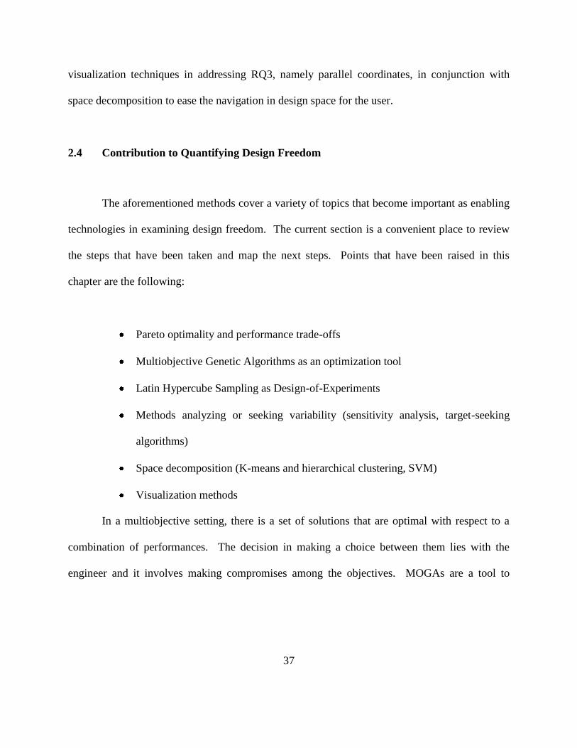
Figure 3.2. Feasible Performances of LH Sampling……………………………………….. 45
Figure 3.3. Latin Hypercube Sample of designs………………………………………….. 46
Figure 3.4. Pareto-optimal performances for the two objectives………………………….. 47
Figure 3.5. Design space for the Pareto-optimal designs………………………………….. 48
Figure 3.6. Pareto and LHS Performances of the studied function……………………….. 48
Figure 3.7. Performance space box boundaries defining a target performance…………… 50
Figure. 3.8. Discretized performances of LHS…...………………………………………... 54
Figure. 3.9. Discretized performances of Pareto set...……………………………………... 55
Figure. 3.10. Discretized LHS designs…...………………………………………………... 55
Figure. 3.11. Discretized designs of Pareto set…………………………………………….. 56
Figure. 3.12. An example of a one-to-one mapping……………………………………...... 59
Figure.3.13. An example of a one-to-many mapping……………………………………… 59
Figure 3.14. Design MEHV for Pareto-optimal and LHS sets…………………………….. 64
Figure 3.15. Average-weighted Performance space location of 6 large MEHVs…………. 66
Figure 3.16. Existing designs in the selected PSB………………………………………… 68
xii
Figure 3.17. Mapped 2-D design space of the selected PSB……………………………… 69
Figure 3.18. Parallel Coordinates of the selected PSB..…………………………………… 70
Figure 3.19. Sample designs………………………………………………………………. 73
Figure 3.20. Sample dendrogram………………………………………………………… 73
Figure 3.21. Branch division in similarity…………………………………………………. 74
Figure 3.22. Navigational process diagram……………………………………….………. 78
Figure 3.23. Hierarchical cluster analysis on the data…………………………….………. 79
Figure 3.24. Validate Mappings ………………………………………………….………. 80
Figure 3.25. K-means application on 4 designs……………………………………….…… 82
Figure 4.1. A visualization of a 2 bar-truss problem………………………………………. 89
Figure 4.2. Performances on the Pareto-optimal front and LHS designs…………………. 94
Figure 4.3. Pareto-optimal designs…………………………………………………….….. 95
Figure 4.4. Design LH sampled designs…………………………………………….…….. 96
Figure 4.5. Design MEHV for Pareto-optimal and LHS sets……………………………… 97
Figure 4.6. Performance space location of large MEHVs…………………………………. 97
Figure 4.7. Performances associated with selected PSB…………………………………... 99
Figure 4.8. Parallel Coordinates representation of mapped designs………………………. 100
Figure 4.9. Hierarchical Clustering, top 3 branches……………………………………….. 102
Figure 4.10. Second level hierarchical analysis on designs. Top 4 branches shown……………………………………………………………………………………… 107
Figure 4.11. Second level hierarchical analysis on designs……………………………….. 109
Figure 4.12. Second level hierarchical analysis on designs……………………………….. 110

xiii
Figure 4.13. Sum of MEHV for Two-Bar Truss…………………………………………… 113
Figure 4.14. Platform for a Vibrating Motor………………………………………………. 114
Figure 4.15. Pareto-optimal front and LHS Mapped Performance sets…………………… 117
Figure 4.16. Design MEHV for Pareto-optimal and LHS sets…………………………….. 120
Figure 4.17. Performance space location of large MEHVs………………………………... 121
Figure 4.18. Performances within the selected Performance Space Region………………. 122
Figure 4.19. Parallel Coordinates representation of mapped designs……………………… 123
Figure 4.20. Hierarchical Clustering on top 5 clusters…………………………………….. 124
Figure 4.21a-e. Validation procedure. Performances in proximity to the PSB……………. 126
Figure 4.22a-e. Validation procedure in Performance Space…………………………….... 128
Figure 4.23. Sum of MEHVs……………………………………………………………… 134
Figure 4.24a. Side view of an I-Beam…………………………………………………….. 135
Figure 4.24b. Cross-sectional view, showing the four variables………………….……….. 135
Figure 4.25. Performance space of Pareto set and selected LHS sampling………………... 137
Figure 4.26. Design space mapped volume for LHS and the Pareto sets ………………… 140
Figure 4.27. Performance space location of large MEHVs……………………………….. 141
Figure 4.28. Selected PSB………………………………………………………………… 142
Figure 4.29. Mapped Designs of Selected PSB…………………………………………… 143
Figure 4.30. Hierarchical clustering with top 7 branches colored………………………… 144
Figure 4.31. Hierarchical Clustering on 12 designs, cluster id8………………………….. 149
Figure 4.32. Designs in the red branch of the hierarchical analysis……………………….. 150
Figure 4.33. Sum of MEHVs……………………………………………………………… 153

xiv
LIST OF USED TERMS
Design: a design configuration described in m real-valued components, �⃑�𝜖ℝ𝑚.
Design Performance: the performance of a design evaluated in n objectives, 𝑓𝜖ℝ𝑛.
Indifference threshold: a variable threshold within which designs are equivalent to each other.
Performance Space Box (PSB): a performance region, 𝑏𝑓𝑗., characterized by indifference
thresholds. It contains a set of equivalent performances.
Design Space Box (DSB): a design region, 𝑏�⃑�𝑖. , characterized by indifference thresholds, It contains a set of equivalent design configurations.
Mapped Designs: design configurations that belong to one PSB.
Mapped Design Range: the variable range of mapped designs, that evaluate to a PSB.
Mapped Envelope Hypervolume (MEHV): the volume formed by the variable bounds of DSBs that mapped designs exist in.

1
1. An Introduction to Design Freedom and One-to-Many Mappings
“The intent of analysis is to design; without design intent the analysis would seem to have
no purpose. […] “Design intent builds intelligence into the analysis.”
- Panos Y. Papalambros, JMD editor (Papalambros, 2010)
The design of engineering systems becomes an elaborate and demanding process.
Engineers are expected to tackle complex tasks in a structured and efficient manner. Design
research provides assistance to engineering decisions through an analysis of the attributes and
corresponding functions of studied systems.
What constitutes design? Papalambros‘s quote has that the ―intent‖ of the analysis is
what constitutes ―design.‖ The assistance the design process provides is the incorporation of
―intelligence‖. The study of design engineering creates value in engineered systems.
The goals of an engineered system vary according to what a consumer seeks and the
environment in which it is anticipated to operate The functionality of a system is assumed to be
measurable through some metric. As a result, designers can evaluate the performance of
multiple designs through the configured system attributes.
Theoretically, similar performances can be obtained through dissimilar designs. A
simple instance is the construction of a rectangle that has an area of 24. This can be achieved
either by rectangles of sides 6 x 4 or 8 x 3: one goal, which has multiple ways to reach it. An

2
obvious and physically relevant example can be given in designing yogurt cups or soda cans that
contain a specified amount of substance but differ in their physical configuration. Complex
engineering systems, such as in the automotive industry, can also exhibit cases where reaching a
goal is possible through multiple designs. This thesis addresses such situations in engineering
design. This is stated through the following definition, which is used within the current thesis:
Definition: Design freedom associates unique performances that are reached by multiple
and dissimilar design configurations
The definition leaves the designer to choose a metric to measure dissimilarity of design
configurations. It can be noted that the given definition is associated and tied to some specified
performance. The definition does not reflect the effects that design variations exhibit on the
system. It contrasts with the definition for design freedom given in (Mistree, 1998), which refers
to ―design freedom as the extent to which a system can be "adjusted" while still meeting its
design requirements‖. Mistree‘s definition is based off a particular design, whose configuration
is ―adjusted‖. In this work, the differences between unique designs with similar performance are
the deciding factor in establishing design freedom.
The purpose of the current chapter is to introduce the motivation and context for the
research. Section 1.1 discusses the motivation for maximizing design freedom. Section 1.2
introduces the reader to the relationship between design and performance spaces and concept of

3
one-to-many mappings. The research questions that drive this work are discussed in Section 1.3.
The steps that are taken in the development of the thesis are described in Section 1.4.
1.1 Motivation for Design Freedom
Suppose that there is a case when multiple and dissimilar designs evaluate to the same
performance. This presents design freedom to the designer. The availability of choices between
alternative design configurations supports the analysis of systems beyond their performance.
Considerable research has focused on multiobjective design optimization and negotiating
trade-offs between conflicting objectives (Kasprzak, 2001, Tappeta, 1997, Mattson, 2004, Wu,
2001, Marler, 2004). Many times, research in this area has referred to the theoretical possibility
of attaining similar performances from multiple, unique design combinations (Chen, 2008),
studied under topics such as ‗design flexibility.‘
The motivation for quantifying design freedom in engineering design is to increase the
number of potential product variants, which increases the ability to customize or personalize. In
a customization context, as defined by Piller and Muller, (2004), three types of customization
exist: style (emotional), fit and comfort (anthropological), and performance (functional). As
product competition increases with continued globalization and consumers look for variation and
individualized products, the advantages of one-to-many mappings become increasingly
important. Significant design space differentiation when examining one-to-many mappings will

4
allow consumers to specify products with similar functionality, yet unique form. Now, imagine a
scenario where customers can define their functional specifications, and are then presented with
corresponding design space information. In cases where a performance space location maps to a
single location in the design space, the customer has limited design freedom in terms of style and
fit and comfort. Conversely, if a single performance space location maps to multiple, diverse
locations in the design space then the customer has increased design freedom with which to
―personalize‖ the product.
Accommodating a set of alternatives in the design space creates the possibility of
considering trade-offs in the configuration choice. Discovering alternatives can create a wide
selection of choices to allow decisions to be taken not only with respect to the computed
performance but also according to the strength of preferences to design configurations. The
benefits of establishing design freedom are the ability to alternate between dissimilar designs
throughout the design process.
This suggests that design freedom can add a competitive advantage in the market
placement of engineering systems. While various efforts have focused on increasing flexibility
in decision making, a review of the current methods in Chapter 3 shows that performance-to-
design space information has not been sufficiently studied. In the current thesis we examine the
value that performance-to-design space mapping brings to quantifying and attaining design
freedom. Obtaining design freedom is achieved through the identification of designs with the
same or very similar performance, while their parameters in the design space are very dissimilar.

5
Such one-to-many mappings between the performance and design space have been previously
hypothesized to yield increased design freedom (Ferguson, 2005ab). They are introduced in
Section 1.2.
1.2 Describing performance-to-design space mapping
This section describes how designs are located in performance space. Given a design
variable vector , and objective functions , this design evaluates to a
multidimensional performance value .
Engineers work in the design space (DS) by selecting designs . This is where the
designer establishes the settings of the system: establishing geometric shape, adding or removing
modules, defining possible platforms, and receiving variable values from other designers. Each
point in the design space is equivalent to a unique design. The performance space (PS),
represented by the functions F1 through Fn, specifies the value of a design with respect to each
objective.
For a given set of mathematical functions describing a system, there exists a one-to-one
mapping between the design space and the performance space. This means that, given some set
of design parameters, the performance of the system can be singularly determined from the
system‘s objective functions. However, the same statement cannot be made when considering
mappings from the performance space to the design space.
6
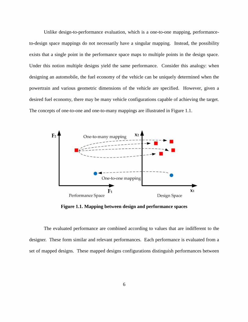
Unlike design-to-performance evaluation, which is a one-to-one mapping, performance-
to-design space mappings do not necessarily have a singular mapping. Instead, the possibility
exists that a single point in the performance space maps to multiple points in the design space.
Under this notion multiple designs yield the same performance. Consider this analogy: when
designing an automobile, the fuel economy of the vehicle can be uniquely determined when the
powertrain and various geometric dimensions of the vehicle are specified. However, given a
desired fuel economy, there may be many vehicle configurations capable of achieving the target.
The concepts of one-to-one and one-to-many mappings are illustrated in Figure 1.1.
Figure 1.1. Mapping between design and performance spaces
The evaluated performance are combined according to values that are indifferent to the
designer. These form similar and relevant performances. Each performance is evaluated from a
set of mapped designs. These mapped designs configurations distinguish performances between

7
one-to-one and one-to-many mappings. For a one-to-one mapping, designs come from similar or
identical designs. Conversely, for one-to-many mappings, designs come from dissimilar or
distinctive designs. The deciding factor is an indifference threshold chosen as appropriate by the
designer. The process allows the designer to consider the bounds of the mapped region in
making informed decisions. These bounds are shown in Figure 1.2.
Figure 1.2. Quantifying the mapped region in the design space
The complex nature of design problems creates a challenge of mapping points between
the performance and design space. Evaluating mappings can be computationally expensive
(Shan, 2010). This feature is mitigated by advances in computational capacity. There is an
opportunity to determine the associated design freedom, given there is access to the evaluated
designs, which are used to compute the variable ranges. The information gained from mappings
can be used in order to examine the research questions on design freedom presented in the next
section.

8
1.3 Research Questions
The analysis of product variations is a valuable part in the consideration of designs
(Olewnik, 2005). Efforts have been pursued by several authors to investigate this possibility
(Chu, 2010, Malak, 2008, Hohm, 2009, Preuss, 2006, Ferguson, 2005ab, Gupta, 2006, de Weck,
2006, Messac, 2000). The current thesis uses the following research assertion in using one-to-
many mappings to quantify design freedom:
Research Assertion. One-to-many mappings exist and identifying them signifies value in
attaining design freedom
The thesis demonstrates the existence of one-to-many mappings in presenting numerical
case study problems. The methodology in applying one-to-many mappings is developed. The
value of one-to-many mappings in quantifying design freedom is consecutively established.
Three principal research questions are formed to address the task of quantifying design
freedom through one-to-many mappings. Particularly, one-to-many mappings close to, and away
from, the optimal region of the performance space will be identified and compared. Assuming
that the mappings exist and are identified, the first research question driving this work can be
stated as:

9
Research Question 1: Do one-to-many mappings located on the Pareto frontier show
significantly less design freedom than those in sub-optimal regions?
This research question requires the comparison of one-to-many mappings located both on
the Pareto frontier, which contains the multiobjective optimal designs, and sub-optimal regions.
Answering this question will provide insight into whether choosing sub-optimal performances
leads to higher design freedom while identifying the necessary performance tradeoffs.
Computational parameters within the research approach can affect the identification of a
subset of one-to-many mapping occurrences. The effect of these parameters must be discussed,
and the importance evaluated, when identifying design freedom. Of particular interest is the
selection of indifference threshold values, which discretize design parameter values. The second
research question is posed to address the use of indifference thresholds given an identified
performance mapping:
Research Question 2: How is the sensitivity of design freedom with respect to indifference
thresholds characterized?
Research Questions 1 and 2 address the implementation of the research approach. The
applicability and value of the results depends on the information that is given to the decision-
making design engineer. This requires a synthesis of the data and the identification of existing
trends. To address this, we first introduce a definition for mapping quality as:

10
Definition: Mapping Quality (MQ) signifies the extent that designs within an identified
region of the design space maps to the original target performance space region
In Fig. 1.2, the reader can note that the area between the mapped designs has ‗gaps‘ of
sampled designs in between. The designs that exist in the region between those designs may not
be associated with the targeted performance. In effect, MQ addresses the effectiveness of the
mapping procedures given a particular set of designs. This leads to the third research question:
Research Question 3: Research Question 3: Can methods be implemented to explore design
choices, in order to identify mapping trends and visualize the data?
The question addresses in what ways the final information on mapped designs
information be used to support designer‘s decisions. Possible avenues in constructing the
research answer include visualization techniques, decomposition and clustering techniques and
design-of-experiments in determining MQ.

11
1.4 Outline of the Thesis
The section examines the direction that the thesis will take and procedure steps that will
be taken in answering the research questions. Section 1.1 established that there is a demand to
categorize design freedom. This is required in order to achieve a greater competitive advantage
through the inclusion of design variability. Section 1.2 showed the mapping relationship
between performance and design space regions when identifying design freedom.
In the following chapter, Chapter 2, the reader will be presented with some available
computational tools and methods. The chapter will also include background information on
related efforts in current research. Chapter 3 presents the methodology that develops mapping
structure when analyzing a problem. Chapter 4 contains 3 test-bed design optimization
examples. Each case-study problem includes information on each research question. Chapter 5
includes a discussion of the method and the thesis conclusion.

12
2. Optimization and Research Background
“There is nothing like looking, if you want to find something. You certainly usually find
something, if you look, but it is not always quite the something you were after.‖
- J.R.R. Tolkien, The Lord of the Rings
Engineering design employs a variety of techniques to analyze, study, and assist the
decision-making processes. This chapter visits prior research efforts that cover design
optimization, design of experiments, sensitivity analysis, tradespace navigation strategies and
visualization techniques. These prior research efforts form a basis into quantifying design
freedom.
Three research questions were posed in Chapter 1. The questions are inspired from the
possibility of analyzing design freedom. Research Question 1 seeks to determine and compare
design freedom between Pareto-optimal and suboptimal regions of the space. Research Question
2 addresses the methodology of the computational process, in particular, what are the effects of
varying indifference threshold size. Research Question 3 addresses the tools and visualization
that support the decision-making process.
The current chapter starts with a review of design optimization. It also presents research
efforts from other analytical fields such as statistics and computer science. The background
provides possible avenues for how similar research questions can be addressed. The literature

13
review identifies that researchers have been interested in studying design freedom and the
generation of design alternatives. However, performance-based approaches have been
overlooked as a suitable tool in determining design freedom. This finding signifies a current
opportunity to employ one-to-many mappings as a performance-based method toward the
quantification of design freedom.
The chapter is split into three major sections. Multiobjective problem optimization is
discussed in Section 2.1. Prior research associated with the topic of design freedom is presented
in Section 2.2. Design navigational tools and visualization methods are placed in Section 2.3.
The design optimization strategies usually involve complex systems with multiple parameters
and objective functions. The next section presents background of optimizing engineering
systems.
2.1 Multiobjective Problem Optimization
The demand to consider complex engineering design problems has increased.
Engineering design employs a set of analytical frameworks in managing product designs. The
use of problem optimization has led to considerable progress in engineering performance (Pahl,
2007). These methods have been developed in a variety of circumstances. The reader can be
directed to the following sources (Pahl, 2007, VanderPlaats, 2005, Park, 2007, Saltelli, 2008,
Azarm, 2006) as references concerning design engineering.

14
Computational developments provide the necessary means to evaluate large-scale
complex engineered systems (Eddy, 2002). This increased problem complexity typically
requires that multiple attributes and decision criteria be considered when choosing a design
configuration. This yields multiobjective problems with often expensive black-box evaluation
costs (Shan, 2010, Lee, 2009, Jones, 1998).
Designs variables represent the attributes, i.e. inputs, of the system being studied. This
thesis assumes that the design variables can be represented as real-valued vectors. Thus, a vector
representing m system attributes is s.t. . Each performance characteristic is represented
as an objective function. Evaluating through functions , where n is the number of
characteristic performances, yields system performance. In the current thesis, we assume that the
objective functions are real-valued and the performances can be presented as
.
The standard form of an optimization problem requires that we minimize all objective
functions while comparing possible trade-offs between the n performances (Vanderplaats, 2007,
Kim, 2006). The form also includes inequality and equality constraints, and
respectively. These constraints define unfeasible regions of the design space in which no
possible solution exists. The formal optimization problem statement is given by Equation 2.1:
(2.1)

15
s.t.
Where
Optimality is not restricted to a singular point due to the possible trade-offs across
performances. The considerations of trade-offs is important for multiobjective problems in
which it becomes an inherent feature. Trade-offs occur when objectives start to compete with
each other. It is common that a particular performance component can be improved only by
sacrificing an improvement in another one. The solution then becomes a set of optimal points
for the combination of performance objectives (Vanderplaats, 2007, Pareto, 1906). The set of
optimal points is called the Pareto-optimal set. A Pareto set consisting of performances P1, P2
and P3 on Pareto front is shown for a generic 2 design variable, 2 objectives problem in Figure
2.1. The performance point P1 performs well in F1 and poorly in F2. Conversely, P3 performs
well in F1 and poorly in F2. The performance of P2 presents a possible trade-off between the two
objectives. The designer can choose any performance on the Pareto with respect to the possible
trade-offs.

16
Figure 2.1. Pareto-optimal front for 2 objective function
In general, the associated design configurations cannot be known until the Pareto set is
computed. There is not a rule to prescribe mapped designs (Shan, 2010). Mapped optimal
designs need not fit a pattern or have an analytical description. Furthermore, the mapped designs
can be very dissimilar to each other and carry large design freedom.

17
However, some problems can contain Pareto sets that map to few selected regions in the
design space. As such, there can be regions in the design space that correspond to optimality
(Preuss, 2007, Shan, 2010). The Pareto frontier or some sub-part of it can have analytical
solutions. Thus, it is possible that some mapped optimal designs can be fit into analytical
solutions or some pattern.
There are multiple issues to consider in optimizing a problem. A way of converging to
the set of optimal solutions has to be found, while constraint violations yield infeasible designs.
Therefore, the design sampling has to be chosen in an effective manner. The following section
covers computational techniques in optimizing multiobjective engineering problems designs.
2.1.1 MOGA Algorithms in Generating Solutions
This section presents methods that seek optimal solutions in multiobjective optimization
problems. A method called Non-Dominated Sorting Algorithm-2 (NSGA-2), an implementation
of a multiobjective genetic algorithm (MOGA), is discussed in additional detail. The NSGA-2
algorithm is employed in the research approach and is described in Chapter 3.
Multiple approaches exist that aim to solve a multiobjective optimization problem. Each
method comes with particular considerations and various degree of accuracy in the search for
optimal designs. Considerable research has been spent on multiobjective design optimization
and negotiating trade-offs between conflicting objectives (Shan, 2010). A simple technique can
18
be devised from the standard problem definition in (2.1) that assigns different weights to each
performance to combine the problem as a single-objective problem optimization. That is an
example of a weighted sum method (Vanderplaats, 2007). Challenges in applying a weighted
sum approach include expanding its performance to non-linear problems, spread of the derived
Pareto set, and computational time in deriving the whole Pareto front. Some other search
techniques are linear programming or stochastic methods such as simulated annealing
(Vanderplaats, 2007, Park, 2007), goal programming algorithms (Deb, 2001), physical
programming (Messac, 2000), or Compromise Decision Support Problem (Mistree, 1995).
Determining and including the robustness of solutions into the optimization has also been
undertaken as a research direction (Li, 2006, Azarm 2006, 2009).
It is important to obtain a representative and high-quality Pareto set. Otherwise,
challenges may arise in the consequent steps of the design process. Discussions on the quality of
different Pareto sets can be obtained in (Deb, 2000, Azarm, 2001, Marin 2009). The metrics that
they introduce focus on finding an accurate and close representation across the whole Pareto
frontier. Some of the metrics (Azarm, 2001) involve representing the Pareto front as widely as
possible without having overlapping performances that would lower the informational content of
the Pareto set.
Even though there is a wide choice of possible algorithms, MOGAs are a particularly
promising option. This is because they show robust performance in black-box optimization
problems (Deb, 2001). Further, they have the ability to form Pareto sets in a single optimization

19
run and are applicable when dealing with continuous and discrete variables. MOGAs can also be
extended to optimization problems with hierarchical structure as well (Kaufmann, 2010).
A distinguishable feature of MOGAs is that they are evolutionary population-based
strategies. The search is performed using a population of designs. Once the population of
designs is evaluated, a new generation of designs is created for the next iteration. Since there are
multiple designs, the population, as a whole, is able to sample and explore large sections of the
design space. This is particularly useful in complex multidimensional problems. In later
iterations, MOGAs exploit the most promising design regions for optimality and converge onto a
solution.
Genetic algorithms refer to design variables as ‗genotypes‘ and the performance as
‗phenotypes‘. These names stem from the origin of genetic algorithms. They were modeled
after genetic recombination (Ebernhart, 2001) and try to mimic the biological adaptation in an
optimization setting (Deb, 2001). The fitness, i.e. goodness, of a design is defined by its
phenotype. The genotype includes the encoding of a particular individual (i.e. design).
The population of individuals has to be initialized. This can be done through heuristic
measures or a database of previously computed designs. A randomly-generated population can
also be used, and once initialized, the MOGA enters a process of iterative adaptation in the
search for optimality defined by fitness.
The population has to adapt through the iterations. There is certainly a wide array of
choices for what actions to take. This is because implementations of GAs differ from each other

20
in both algorithm architecture and in its resulting performance. There are three common steps
among GAs:
Selection: the choice of which designs to base next generation on. Some of the
designs, usually the more optimal ones, are used in generating the next-turn‘s
population.
Crossover: in creating the next generation, the genotype of the new designs has to
be chosen. The information of the designs that passed the selection phase is
used. This ensures that the high-performing genotypes remain within the
population. The crossover stage exchanges variable information between
designs.
Mutation: the step randomizes an individual‘s phenotype. This ensures
variations are introduced into the population. This process allows for exploration
of unsampled regions of the space.
After the designs have been selected, their genotype is crossed between two parents and a
number of offspring. This allows a population of designs that sample the design space to search
for both local and global minima. Here the phenotype drives the fitness and the search is
performed by changing the genotype.
Computational complexity has been an issue that MOGAs have to address in order to
reach solutions within manageable time. Discussions on this topic can be found in (Deb, 2001,
Jones, 1998). The size of the population influences algorithm performance. GAs also contain

21
stochastic elements and this makes their analysis dependant on numerical runs. Therefore, it has
been suggested to run an optimization more than once to ensure that the optimal solution has
been obtained (Vanderplaats, 2009).
The type of algorithm and implementation clearly affects the optimization process.
Among the algorithms, and of particular interest, is the Non-dominated Sorting Genetic
Algorithm-2 (NSGA-2), as shown in (Deb, 2000, Deb, 2001, Deb, 2002). The differences
between NSGA-2 and other MOGAs include methods of working with dominated solutions and
consequent crossover between solutions. NSGA-2 preserves a number of individuals with the
highest fitness onto the next iterations, making it an elitist MOGA. It uses sorting to compare
performances between multiple dimensions of the individuals in the population. Its complexity
in sorting through the solutions is given as ( ), where n is the number of objectives and z is
the size of the population (Deb, 2002). Furthermore, it also includes niching techniques that
preserve design diversity (ibid).
Diversity preserving requirements presents features of MOGA algorithms that clarify
some aspects of their procedures. Optimization strategies involve either a single design, which is
iterated to more optimal values, or a population of designs which sample the space in a parallel
fashion (Vanderplaats, 2007). The iterative, one-design-at-a-time optimization might converge
prematurely to an underperforming design (Deb, 2001, VanderPlaats, 2007). On the other hand,
population-based strategies can evaluate multiple designs in a single iteration. The use of a
population affects the sampling by having more options to ‗explore‘ different regions of the

22
space and to seek solutions that can yield better optimal values. The process is aimed at avoiding
local minima (Deb, 2001). Given a region of interest, the ‗exploitation‘ stage finds and
converges onto the best solution within the region. While the size of the population clearly
affects these processes, no clear-cut boundaries are established due to the stochastic aspect of
optimization (Deb, 2001). The diversity of the population is important, especially in the
‗exploration‘ aspect of the optimization process.
Goldberg and Deb show the use of diversity in developing genetic algorithms and
techniques. (Goldberg, 1989). They developed the use of ‗niching‘ techniques that use measures
of the spread of solutions in either phenotype (performance) or genotype (design space). The
step measures distances between points in the population sets in either one of the spaces
achieving a high coverage of solutions with the goal of avoiding similar designs.
There are three main reasons to select the NSGA-2 algorithm: 1) the code is robust and
easily configurable to a variety of engineering problems; 2) the algorithm was shown to
generally outperform other MOGA algorithms (Strenth Pareto Evolutionary Appoach -1 (SPEA-
1), Vector Evaluated Genetic Algorith (VEGA) and NSGA-1, (Deb, 2001)); and 3) the algorithm
has been introduced as part of available software packages.
Matlab‘s optimization toolbox contains the gamultiobj function, which is an
implementation of the NSGA-2 algorithm. Furthermore, a flexible and efficient source-code
package is provided by Sastry (Sastry, 2007). The code was developed at the Illinois Genetics
Algorithm Laboratory. It does not have explicit restrictions in generating large Pareto set
23
populations, which can capture the Pareto frontier very closely. The code is, therefore,
implemented in the research approach in finding the Pareto set. This is presented in Chapter 3.
2.1.2 Design of Experiments Methods in Sampling
Design of Experiments (DoE) refers to methods that generate suggested designs in the
sampling of a problem. They can be used in determining function‘s behavior and identifying
influential variables in an effective manner. The most basic sampling technique is probably grid
sampling or grid search (Vanderplaats, 2007). Along a given dimension, it places test designs a
uniform distance from each other. As a number of designs are evaluated, it can exhaustively test
a problem. The method is not advised as an efficient manner to test black-box problems. Large
regions of the space need not contain any additional information concerning the problem, as they
can be associated with less sensitive or non-influential variables. Therefore, for computationally
expensive problems, sampling a grid can become time prohibitive for an effective search.
Different strategies have been devised to avoid this problem.
Research in DoE methods has developed more efficient approaches, and the reader is
directed to (Saltelli, 2008) for further information on available options. These include the use of
randomized variables that sample the problem in a non-uniform way, Fractional Factorial and
Stratified Multivariate methods to test combinations of multidimensional parameters (ibid).

24
One possible choice is the use of Latin Hypercube Sampling (LHS), which has been
investigated in engineering design successfully (Chen, 2009). Here, an individual variable can
be stratified, or split, into different test intervals. This creates a series of non-overlapping
regions that represent the domain in a uniform fashion and is suitable for test sampling. LHS
design uses such intervals as one of its main features, in that it splits the domain of each
dimension of a multivariable problem into the same number of intervals, s. Within a given
interval, chosen for sampling, the method assigns a design through some calculation. For
example, thr lhsdesign function in Matlab uses randomly generated designs within each interval
as its default setting. A key feature of a definition of a LHS design is that the test designs are
chosen to sample any direction of the domain the same number of times. For a 2 dimensional
grid, this forms a Latin Square – hence the name, Latin Hypercube Sampling. Such a sampling
technique reduces the uncertainty in the obtained performance compared to a generalized
randomized sampling. These features make it a common sampling procedure and it is
incorporated in the research approach.
2.2 Analysis of Design Alternatives
Multiple strategies of generating alternative designs have already been pursued. They are
applied at different circumstances to analyze the particular aspects that each method is interested
25
in. This section will cover several topics in design variations and alternatives. Presented topics
are listed below:
Target approximation through Design of Experiments
Set-based design
Target-Seeking and alternatives generation
Sensitivity and robust analysis
2.2.1 Target Approximation
Performance regions have had to be approximated and analyzed for a variety of reasons.
In reliability analysis (Bertsche, 2009), regions that lead to failure are avoided. The performance
space, therefore, has to be characterized with particular attention to the boundaries between
regions that have to be avoided and those that have to be optimized (Picheny, 2010, Ranjan,
2008).
Recent work (ibid) proposes a sequential design of experiments methodology to
approximate target performance regions. The work is concerned with the efficient selection of
designs to determine the boundary separating regions. The work finds and samples a target
performance region in an efficient design-of-experiments manner. This establishes information
related to design freedom. The work does not, however, address alleviating the subsequent
design decisions.

26
2.2.2 Set-based design
Set-based design approaches (Finch, 1997, Chen, 1999, Chen, 2008a, Shan, 2004, Sobek,
1999) have been used in concurrent engineering environments as a means of maintaining
opportunities to change designs at a later stage. In comparison to the definition given in Chapter
1, this quality is also sometimes referred to as design freedom (Chen, 2008a).
Set-based design involves making decisions between sets of possible designs. It
therefore maps a region of design space to a region of the performance space. Through the
design process, the decisions are adapted and a single design is chosen as information about the
system accumulates. Motivation for this approach is to delay the need for making design
commitments until later in the design process.
Recent work (Madhavan, 2008) has shown that in an industrial setting, set-based design
approaches reduce the number of iterations between design teams and provide a library of back-
up design options. Research in target sets to decompose the design space and identify optimal
solutions was conducted in (Chen, 2008a). Physical Programming methods developed in (Chen,
2000, Messac, 2002) differentiate solutions into five different types based on the quality of the
solution, considering all solutions within the same type equivalent.
However, such approaches are typically driven by design space decisions in an effort to
converge to a single solution. Therefore, they do not correspond straight-forward to the analysis

27
of design freedom. The analysis of design freedom can be adjusted to yield sets of possible
options within some measure of equivalency, making it similar to Physical Programming.
2.2.3 Target-seeking and Alternative Generation Algorithms
This section introduces target-seeking algorithms and techniques that seek alternatives in
the design space. A common method to find unique solutions with a similar performance is
through a two-level optimization. The first run determines the performances that are optimal or
functional. The second run of the optimization contains the objective to minimize the deviation
in performance while maximizing the distance between designs. Such approaches are commonly
referred to as target-seeking or goal-seeking algorithms.
2.2.3.1 Modeling to Generate Alternatives
A target-seeking algorithm can change the objective function to quantify the distance to a
target value. A recent approach devised for target-seeking is Modeling to Generate Alternatives
(MGA) published in (Brill, 1983, Gupta, 2006). This approach constructs an optimization
problem to find candidate designs that are farthest away from each other in the design space by
relaxing desired system performance. This constraint frames a boundary in the performance

28
space around the optimal value but within which performances are acceptable. This can be
envisioned by building a ‗box‘ around the targeted region.
2.2.3.2 Parameterized Sets
The search for alternatives in decisions trees has been recently pursued by Paredis and
Malak. The design freedom framework as defined in (Malak, 2008a) and (Malak, 2009) is based
on a tree of decisions that design engineers take in the process of product development. Design
freedom becomes the ability to reach appropriate performances by backtracking on the decisions
leaves. The approach has potential to grow into a more extensive framework for exploring and
characterizing engineering decisions. One aspect of their research is the use of support vector
machines (SVM) in identifying domain regions which can be extended to other predictive
engineering environments. Nevertheless, the authors work outside the design space. This
impedes its integration for functional analysis of design freedom.
2.2.3.3 Inverse Design and Isoperformance
In plotting the performance in a problem, it is convenient to use performance contours in
the display. If we form a mathematical description of an isoperformance contour, we will be
presented with the opportunity to determine which designs evaluate to the same performance.

29
De Weck (2004) has introduced the notion of isoperformance, in which a formulation for
efficient level sets of designs with similar performance is presented. This work uses the Jacobian
of the inverse matrix to generate the contours. These are then used to evaluate the design
concepts, while also evaluating the constraint restrictions. A possible practical issue is that
black-box problems might not have easily accessible Jacobians.
2.2.3.4 Design Diversity in Evolutionary Algorithms.
The current section reviews the process of using design diversity in computational
frameworks of evolutionary algorithms (EA). MOGA belong to EA and they are introduced in
the earlier section 2.1.1. Different EA, and in particular MOGAs, employ design diversity, a
measure of variations that exist in a given design population, in the process of solving for
optimal solutions.
The use of diversity in computational frameworks creates an analogy for design freedom
in a computational setting. It has shown benefits in the optimization process (Deb, 2001,
Vanderstaal, 2008, Ehrgott, 2009). Sampling the space, while preserving design diversity, is a
computationally efficient method to explore the design space. It presents the potential that the
use of diverse sets of solutions is able to achieve.
Some recent computational research (Preuss, 2009, Beninni, 2003) uses diversity as an
objective to explore the possibility of having multiple design solutions to a performance.

30
Diversity-seeking algorithms have a potential in generating solutions with high level of design
freedom.
A method is presented in Hacker (Hacker, 2001) which aims to determine the modality of
a problem. The research changes the exploitation stage of the optimization. This approach
computes the variance of the population in both performance and design space. This information
is used to choose a strategy for exploitation of a performance space at any given stage of the
optimization. It is an example of using a diversity-dependant strategy in improving the
optimization process.
An earlier work, (Bennini, 2003) treats diversity as an individual objective to steer the
population to higher design freedom. The method involves assigning a diversity measure to the
individuals in the population and using it in the selection stage of the algorithm. The effect is to
assign an additional fitness measure.
Computational methodologies have also paid attention to design diversity and
performance-to-design evaluations. The review of the research efforts shows the cross-
disciplinary nature of design freedom. The current thesis does not implement diversity-seeking
MOGAs. This is done to present the sampling information back to the designer in a more
deterministic fashion.

31
2.2.4 Sensitivity Analysis
This section covers applied and analytical methods into robustness and sensitivity
analysis. The goal of these approaches is to characterize the effects that design variables changes
have on performance. Robust design is aimed at reducing performance changes due to
uncontrollable variations of a design. Sensitivity analysis is a field of study that aims to identify
contributing factors into performance variation through a far-reaching statistical and scientific
background (Cacucci, 2003, Saltelli, 2008, Giassi, 2004, Goh, 2007, Turner, 2007, Yin, 2008). It
uses DoE sampling to test problems and characterizes the variations in performance to identify
the most influential parameters given a particular effect. In (Saltelli, 2008), a study is performed
on a batch reactor to identify when a thermal runaway occurs. It is an undesirable event to be
avoided in practical applications. The study extends to determine which factors contribute to
minimize the possibility of this event through regression models. Robust design, on the other
hand, can improve reliability in applied engineering systems (Azarm, 2005).
Significant research has been directed at characterizing the effect design variables
variations have on performance in order to assess possible performance degradation. These
variations arise due to manufacturing tolerances, wear time, or further factors which have an
effect on reliability and performance (Bertsche, 2010). Azarm et al. use regionalized sensitivity
analysis (2005) to develop robust solutions. Interval-reduction measures have been taken in
(Azarm, 2009) to achieve reliable solutions.

32
Even though these aforementioned methods have a wide use, the authors have not
encountered a sensitivity analysis aimed at design freedom originating with performance values.
2.3 Navigation in Design Space
Sampling designs and optimizing the solutions can lead to a large amount of information
regarding the solutions. The decisions that designers have to make become a demanding task for
complex engineering systems. This is due to the high number of decision variables and problem
complexity. The abundance of information can create a bottleneck for the designer by
obstructing some of the underlying structure. For example, a human can usually rationally
consider up to 7 pieces of information at once (Eysenck, 2005).
This section deals with existing issues of navigating the design space. The section is split
in two sub-sections: investigating structural information through decomposition techniques; and
visualization techniques used in design research.
2.3.1 Space Decomposition Research
Space decomposition can be used to enhance the decision-making abilities of the designer
by structuring the data effectively (Arenbeck, 2010, Kuczera, 2009, Lu, 2009, Wang, 2006).
This lies at the center of addressing RQ3. The current section discusses ‗similarity‘ through
33
space decomposition techniques that classify or group parameters of designs. The current
section investigates what methods exist to relate the performance-to-design spaces and whether
they can be applied to address RQ1 and RQ3. The methods presented herein include K-means
clustering, hierarchical clustering, artificial neural networks and support vector machines.
An important research direction, listed in (Shan, 2010), is the ability to differentiate
design regions with respect to their potential performance values. Optimal regions are
commonly confined within a small area of the design space. Identifying the useful regions in a
problem could increase the effectiveness of search algorithms. Furthermore, optimization
strategies can potentially benefit from classification techniques through the use of correlation
among parameters.
An option of partitioning the design space is using rough sets theory. Rough sets apply
thresholds in decomposing the design spaces. The partitioning is assigned according to
performances from designs of the associated regions. The final result maps target performance
to associated design regions. The research is shown in (Chu, 2010, Chen, 2007, Shan, 2004).
The process is aimed at multidisciplinary complex designs.
Clustering methods emerge as particularly useful in grouping and identifying patterns.
Zitzler (2008) worked to determine which variables were associated with the solutions on the
Pareto-optimal front and how similar these designs were. Their approach was to use hierarchical
clustering techniques to identify modules of principal structural information applied on Pareto-
optimal designs. This method clusters and groups the designs in a hierarchical manner resulting

34
in a dendrogram. Here, the leaves are the final designs and intermediate branches signify
common features among the dataset of designs.
In hierarchical clustering, similarity between designs, or a group of designs, is first
computed (Karypis, 2004). The information generates a similarity matrix that contains distances
between designs. Starting from individual designs, which form the leaves of the dendrogram, the
data is then repetitively merged into larger groups. A larger group corresponds to a higher level
in the branch tree. For a binary tree, the data is combined to a single branch.
One method to unite groups of designs together is to evaluate the shortest distance
between elements of each two branches. The metric is called ‗single‘ within Matlab. A node is
then constructed by merging the branches that are closest to each other. In the unweighted
average distance (UPMGA) metric, the distance between every member that belongs to two
different branches of a tree is computed to evaluate the distance between these two branches.
The two branches with the smallest distance are then united in a branch of one level higher.
Clusters can then be further derived on the ending branches of the tree that form groups.
Another common clustering algorithm is K-means (ibid). The supplied data has to be
split into k-number of clusters, hence the name, K-means. The objective is to have the centers of
the clusters represent the data appropriately and identify the existing clusters. The method
requires that a ‗seed‘ of cluster centers is placed on the set of designs, and that each design is
assigned to the nearest center of the cluster. The initial placement of cluster centers can be
randomized. The centers can be designs from the data or the centroid of a group of data. The

35
centers are updated in consecutive iterations. The objective is to minimize the total distance from
within the designs to their assigned cluster centers and maximize the distance between clusters.
The metric to measure distances is chosen by the user. The algorithm is stochastic, whereby a
single run might be stuck in local minima. It is suggested that multiple runs are performed to
confirm the cluster distribution. In searching for a balanced representation, it is also advisable to
have multiple runs with different number of clusters.
2.3.2 Visualization Research
This section introduces current visualization tools that are used to represent the complex
information associated with a design‘s configuration. Several approaches have been developed
that communicate the data related to a problem, which include solutions and allow for interaction
with the human decision-maker (Eddy and Lewis, 2002, Frecker, 2009, Naone, 2010,
Shneiderman, 2006, 2007, Wolf, 2009). Scientific and information fields use visualization to
exchange complex information (Wolf, 2009) and visualization procedures are undergoing further
research development.
Interactive procedures can analyze and display trends in large data-driven information
settings. In a current news article, the author (Naone, 2010) presents two visualization methods
that carry general-purpose interactive settings. One is Pivot (ibid), a Microsoft product that
displays data from databases with both graphical and textual information. Another competing
technology for large visual displays is Many Eyes from IBM (ibid). These technologies include

36
multidimensional scatter plots, network graphs and textual analysis. These methods can be used
to relay complex information interactively to a user.
The requirements for design visualization suggest the use of interactive methods in an
engineering environment. Frecker and Finger present (Frecker, 2009, Frecker. 2009) the use of
DesignWeb, an interactive navigational design toolbox. Their research uses it for the
summarization of knowledge, reuse and analysis of designs. One of its capabilities is creating a
graph representation of core concepts and generating relationships between them using textual
analysis and clustering algorithms.
Visualization systems have to allow for the analysis of performance attributes while
navigating the design space. A ‗Design by Shopping‘ approach (Wolf, 2009; Eddy, 2002)
samples the design space and then allows designers to pick regions they want to explore further.
Another type of design visualization is explored through the Applied Research Laboratory Trade
Space Visualizer (Wolf, 2009, Simpson, 2004, 2008). Simpson et al. studied representation of
MultiDimensional and MultiScale Interactions and used ATSV to navigate through a complex
interacting design space. It is capable of visualizing multidimensional data by plotting all of the
designs. This process fosters the identification of major trends in the data visually, such as the
existence of clusters of data.
Visualization techniques are necessary to relay information to the designer so that
rational, informed decisions can be made. The research in this thesis investigates and uses
37
visualization techniques in addressing RQ3, namely parallel coordinates, in conjunction with
space decomposition to ease the navigation in design space for the user.
2.4 Contribution to Quantifying Design Freedom
The aforementioned methods cover a variety of topics that become important as enabling
technologies in examining design freedom. The current section is a convenient place to review
the steps that have been taken and map the next steps. Points that have been raised in this
chapter are the following:
Pareto optimality and performance trade-offs
Multiobjective Genetic Algorithms as an optimization tool
Latin Hypercube Sampling as Design-of-Experiments
Methods analyzing or seeking variability (sensitivity analysis, target-seeking
algorithms)
Space decomposition (K-means and hierarchical clustering, SVM)
Visualization methods
In a multiobjective setting, there is a set of solutions that are optimal with respect to a
combination of performances. The decision in making a choice between them lies with the
engineer and it involves making compromises among the objectives. MOGAs are a tool to

38
identify the Pareto front effectively, while LHS samples the design space to yield an informative
representation of the associated performance space. Displaying the solutions allows decisions to
be made effectively. Nevertheless, conveying the data for highly dimensional problems becomes
a hard issue itself. Clustering can capture the information of the mapped designs to identify
principal properties. The information is given this information in taking decisions more
effectively.
The next chapter will be a review of research efforts into design freedom and the use of
mapping information to quantify it. The inclusion of the next chapter will encompass the
necessary background to describe the research approach, described in Chapter 3. The research
approach is going to be tested on several case study problems and be presented in Chapter 4.

39
3. Research Approach
“Begin at the beginning and go on till you come to the end: then stop.”
The King, In “Alice in Wonderland”, Lewis Caroll
In this chapter, the research approach proposed in the thesis is outlined and discussed.
The approach in Figure 3.1 is used to locate and analyze one-to-many mappings in
multiobjective engineering problems. To facilitate the discussion of the approach, a sample
problem – ZDT-3 (Zitzhler, 1999) – is simultaneously presented.
Figure 3.1. Research approach

40
The proposed research approach to analyze design freedom contains a series of 8 steps.
They are broken down into four major components, which are described below:
I. Sample Designs: Sample designs to obtain information on the performance values
II. Obtain PS-to-DS data. Generate inverse data from the performance (PS) to
design space (DS). This step identifies mapping types and quantifies design
freedom of selected locations in the performance space.
III. Rank and Compare sets. Rank the performances according to design freedom and
compare design freedom across different locations in the performance space.
IV. Design Navigation: Visualize design variables and identify mapping trends to
guide user decisions. This step supports designer decision making through
validating mapping information and clustering designs.
The steps of the approach take the user from generating solutions to the process of
decision making in system design. The steps are presented separately to signify that they are
computationally independent of each other. The following section, 3.1., starts the description of
the research approach with an explanation how to generate a number of feasible designs.

41
3.1. Sampling the Design Space
The research approach requires that feasible performances are found. There are two sets
of designs that are deemed of interest within the thesis. One is the set of Pareto-optimal designs.
This set consists of highly-optimal designs, which designers identify to avoid inferior products.
The other set of designs is chosen so that it covers the range of performances which are
achievable in the multiobjective optimization problem, even if they are dominated designs.
This explanation begins with a review of the definition of a function. A function is a
mapping between a variable that belongs to the domain of a function, to the range of the function
(Lay. 2000). In the context of the current thesis, a function maps from design space to
performance space. The function can be described either as a formula that describes the
mapping, given in (3.1a), or through a mapping itself, given in (3.1b). It is assumed that a design
can be presented as a vector of real numbers, , with performances given as
multidimensional vectors of real numbers, .
(3.1a)
(3.1b)

42
Sampling designs of a given problem fills the mapping information in Equation (3.2).
The first step of the research approach chooses how to sample the design space of a given
multiobjective optimization problem. The choice occurs between the two objectives that are of
particular interest, 1.) seeking optimal performances or 2.) seeking higher design freedom in
dominated performances.
(3.2)
To identify a problem‘s Pareto frontier, MOGAs have been shown as an effective
approach. They show robustness in generating optimal solutions in multiple settings, for both
continuous and discrete problems. To optimize efficiency and evaluate a large number of
designs, the thesis uses a software package from Sastry (Sastry, 2006) in identifying Pareto-
optimal designs.
Pareto-optimal designs are frequently confined within a small region of the design space
(Shan, 2007). The performance space also includes a very large proportion of feasible but
dominated or sub-optimal performances. To test for design freedom, a method has to be chosen
to sample feasible designs. The chosen method is Latin Hypercube sampling (LHS), discussed
in Chapter 2 (Saltelli, 2008, Chen, 2000, Montgomery, 2008). LHS is able to generate a list of
designs to be evaluated that effectively represent the possible performance space.

43
The research approach uses the two sets of designs that result from each method. The
range of evaluated designs is 5000-10000 which is kept in the same order of magnitude between
the two sets of designs. The design population is kept constant at the target level throughout the
MOGA optimization. Thus, the population stays at q = 5000 or q = 10000 during the
evolutionary stage. At the end of the optimization, any infeasible designs are discarded.
Under LHS, a list of designs configurations is generated which are first evaluated for
feasibility. For example, for a target range of q = 5000 designs, a list of 1000 designs is
generated and evaluated for infeasibility. The feasible designs are saved and a new list of 1000
sample design is generated and checked for feasibility. The process is continued until the target
number of designs is reached or exceeded. Therefore, the LHS set can slightly overshoot the
target number of designs.
The current sampling step completes the exploration of the multiobjective problem. The
evaluation of sets of sampled designs allows us to consider performance-to-design information.
In it, the binary pair ( is instead numerically presented as ( . The process is elaborated
on in Section 3.2. The current step is illustrated on an example problem.
Application to a simple optimization problem
An investigation is conducted and presented on a mathematical test-bed problem to
demonstrate the steps of the approach. Zitzler, Deb and Thiele have investigated optimization

44
strategies and in (Zitzler, 2000) introduce a set of 6 test-bed optimization problems. This section
presents initial analysis on a problem from the set, ZDT-3. The version presented in Equation
(3.3) is an unconstrained multiobjective problem with two objectives and two design variables.
(3.3)
For
The Latin Hypercube performances of the problem are presented in Figure 3.2. The
samples are over the domain of the problem, for and . They are presented in
Figure 3.3. The problem is unconstrained and therefore every sampled design on the domain is
feasible. The sample set consists of 5000 designs. The feasible performances cover a range of
[0, 1] in F1 and a range of [-0.772, 9.44] in F2.
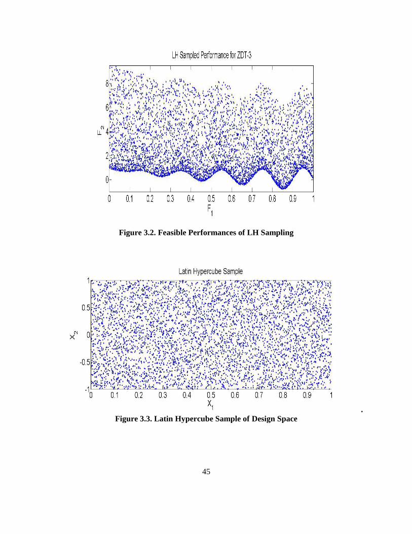
45
Figure 3.2. Feasible Performances of LH Sampling
.
Figure 3.3. Latin Hypercube Sample of Design Space

46
The next sampling is an optimization procedure using the MOGA toolbox, supplied by
(Sastry, 2006). There is a limit of 200 generations, after which the algorithm terminates. The
design population is initiated through a random generation. The population size is set at 5000.
The population undergoes 200 generations. In each generation, half of the designs are modified
to explore for optimal values in new regions of the space. The supplied optimization toolbox,
GAtbxm, requires a configuration file with the necessary input variables. The file is included in
Appendix A.
The Pareto-set is shown in Figure 3.4. The Pareto-optimal performances cover a range of
[0, 0.8518] in F1 and a range of [-0.773, 1] in F2. The range of optimal performances in F2 is
significantly smaller for the Pareto-optimal set than for the LHS designs. The design space is
shown in Figure 3.5. The generated set of optimal designs occupy a range of [0, 0.8518] in X1
and [-0.0058, 0.0099] in X2. The domain of the problem is [0, 1] in X1 and [-1, 1] in X2.

47
Figure 3.4. Pareto-optimal performances for the two objectives
Figure 3.5. Design space for the Pareto-optimal designs

48
Figure 3.6. Pareto and LHS Performances of the studied function
The two performances are shown together in Figure 3.6 illustrating how the two sets of
sampled performances extend over the region. The Pareto set identifies a discontinuous front
along the LHS performances, and is concentrated to a small region of the performance space.
The LHS performances include dominated designs that exist in the suboptimal performance
regions beyond the Pareto-optimal front.

49
3.2. Indifference thresholds discretization
The thesis uses indifference thresholds in quantifying design freedom. Designs are
considered equivalent if they belong to a target hyperbox, which is characterized by a specified
indifference threshold limit. The process is shown in (Ferguson, 2005ab). The step is used on
both the performance and design variables.
Consumers can find themselves in a position to consider some similar performances to be
equivalent. An example can be given for a customer comparing fuel economy of car models. A
person with an indifference threshold of 1 MPG would not differentiate between cars that are
listed to have 25 MPG or 26 MPG. A customer can find mileage information on the site
fueleconomy.gov, which lists the mileage of a 2.4 L, 4 cylinder 2010 Chevrolet Malibu is
rounded to 26 miles per gallon for a combined driving test cycle. The mileage for 2.5L 4
cylinder 2010 Ford Fusion FWD is listed as 25 MPG. For the example customer, these
performances are within their desired target performance and therefore they are equivalent to
each other.
Consider the case for the performance in a two objective problem, shown in Figure 3.7.
The designer chooses a two-dimensional indifference range vector , that has two components,
RF1 and RF2. The indifference threshold is used to create boundaries of target performances.
Any performance that is within the performance space box (PSB) is equivalent to the specified
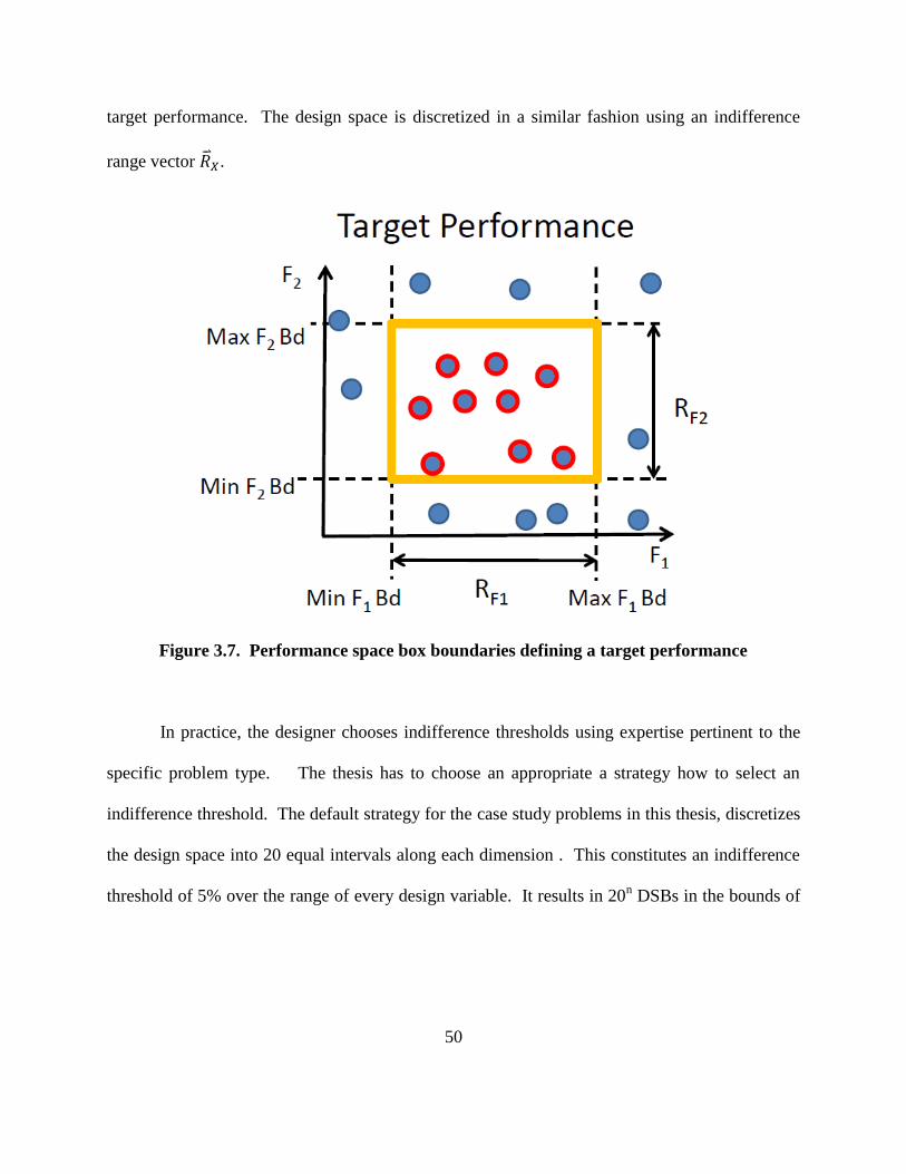
50
target performance. The design space is discretized in a similar fashion using an indifference
range vector .
Figure 3.7. Performance space box boundaries defining a target performance
In practice, the designer chooses indifference thresholds using expertise pertinent to the
specific problem type. The thesis has to choose an appropriate a strategy how to select an
indifference threshold. The default strategy for the case study problems in this thesis, discretizes
the design space into 20 equal intervals along each dimension . This constitutes an indifference
threshold of 5% over the range of every design variable. It results in 20n DSBs in the bounds of

51
an n-dimensional domain, ( . While investigating Research Question 2, the indifference
threshold setting is varied between 0.1% to 10%.
To choose a performance indifference threshold, we assume a set of evaluated mappings
M, as constructed in Equation (3.2), is already generated. The set can consist either of Pareto-
optimal designs or feasible designs generated through LHS. For each set, the performance range
is calculated as the multidimensional upper and lower bounds of performances ( . The
indifference threshold is set at 5% of the range of each objective. It creates 20m
hyperboxes in
the m-dimensional space of considered performances in each set of mappings, M.
The indifference threshold values are therefore dependant on the particular set of
mappings being studied. Nevertheless, the number of performance and design space boxes stays
constant. The mappings cover different performance regions and therefore the indifference
thresholds are scaled to correspond to the different regions.
The application of hyperboxes is given by distances from the centroid points in each
particular box. There are 20m
such points in performance space. The target centroid points in
design space are 20n. Equation (3.5) describes how to construct each point, indexed under j and
k respectively.
= (3.5a)
= (3.5b)

52
For a hyperbox, in performance space, any performance within the performance
indifference threshold maps to it, . Equation (3.6a) is a mapping function that groups
the performances within the hyperbox bounds. Similarly, Equation (3.6b) maps indifference
threshold discretizations in the design space.
(3.6a)
(3.6b)
The process groups equivalent performances together, while permitting the differentiation
between dissimilar design configurations. Effectively, a mapping is created for each design
between hyperboxes in the performance space and design space. Consequently, is
presented as where and . The hyperboxes retain the same
dimensionality of the original corresponding DS and PS, but exist in integer space. The mapping
is then inverted to obtain the following performance-to-design space structure, as shown in
Equation (3.7).
(3.7)

53
The discretization process quantifies design freedom in a 1-norm distance metric in both
performance and design space. The designer assumes that customers measure performance
within the performance indifference threshold. Furthermore, the designer assumes that
differences in physical configurations are measured in each variable separately up to the design
space indifference threshold.
Designers have the opportunity to uniquely define and modify hyperboxes in both the
design space and performance space. The hyperbox mapping, as in Equation (3.7) can be
extended to include some general functions and according to their individualized
computational preferences. The function is generic to allow the designer to specify how to carry
the step. The functions can be defined depending to the particular design application as in
Equation (3.8).
(3.8a)
(3.8b)
Application to a simple optimization problem
We apply this step to the example problem begun in the last step which is represented by
Equation (3.3). The two sets of mappings with Pareto and LHS designs are treated separately.
The discretization of the performance space is shown in Figure 3.8 for the LHS and Figure 3.9

54
for the Pareto set. The grid in each figure signifies the bounds of the different hyperbox regions.
The problem is two dimensional in both design and performance space. Therefore, both design
and performance spaces are discretized into grids of 202 = 400 hyperboxes.
Figure. 3.8 Discretized performances of LHS
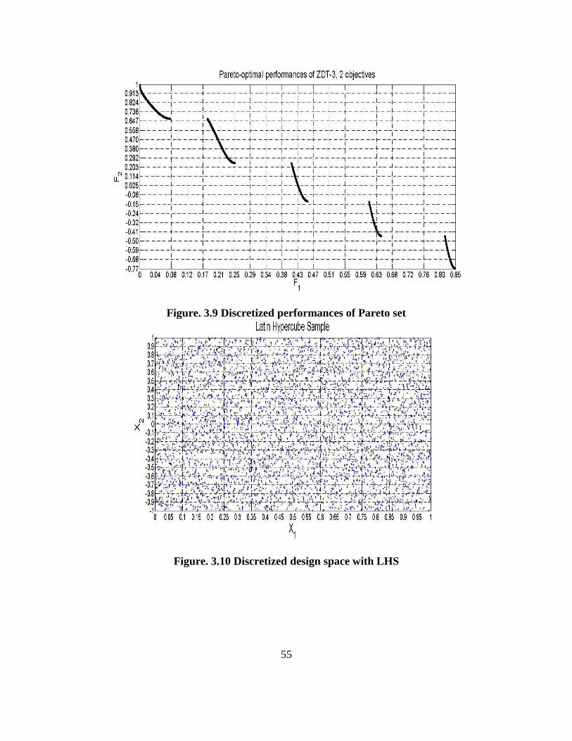
55
Figure. 3.9 Discretized performances of Pareto set
Figure. 3.10 Discretized design space with LHS
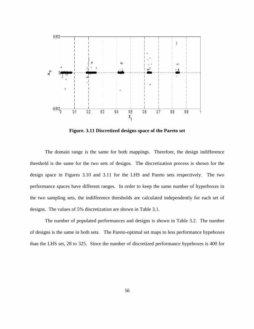
56
Figure. 3.11 Discretized designs space of the Pareto set
The domain range is the same for both mappings. Therefore, the design indifference
threshold is the same for the two sets of designs. The discretization process is shown for the
design space in Figures 3.10 and 3.11 for the LHS and Pareto sets respectively. The two
performance spaces have different ranges. In order to keep the same number of hyperboxes in
the two sampling sets, the indifference thresholds are calculated independently for each set of
designs. The values of 5% discretization are shown in Table 3.1.
The number of populated performances and designs is shown in Table 3.2. The number
of designs is the same in both sets. The Pareto-optimal set maps to less performance hypeboxes
than the LHS set, 28 to 325. Since the number of discretized performance hypeboxes is 400 for

57
both sampling types, the number of populated performance hyperboxes for the Pareto set is 7%,
while the LHS set achieves 81.25%.
The number of populated design boxes and sum of populated mapped boxes is shown in
Table 3.2. Each DSB that has a design in it is considered populated. Clearly, the Pareto designs
are much more densely populated, with only 21 DSB filled, which is 5.25% of the available
design space hyperboxes. The set of LHS designs covers all but one of the possible DSB.
Each unique performance is associated with a number of mapped design boxes. The sum
of DSB over every performance is also shown in Table 3.2. The performance hyperboxes of the
Pareto set map back to a total of 68 design space hyperboxes. The performances of the LHS set
map back to a total of 1128 design space hyperboxes. This signifies that unique performances
map to multiple design space hyperboxes for each sampling type. This is an example of one-to-
many mappings, described in the next section.
Table 3.1. Results from performance space discretization
Pareto-
optimal set
Latin
Hypercube
sampling
Number of designs 5000 5000
Threshold size in F1 0.0426 .05
Threshold size in F2 0.0887 0.5113
Populated hyperboxes 28 325
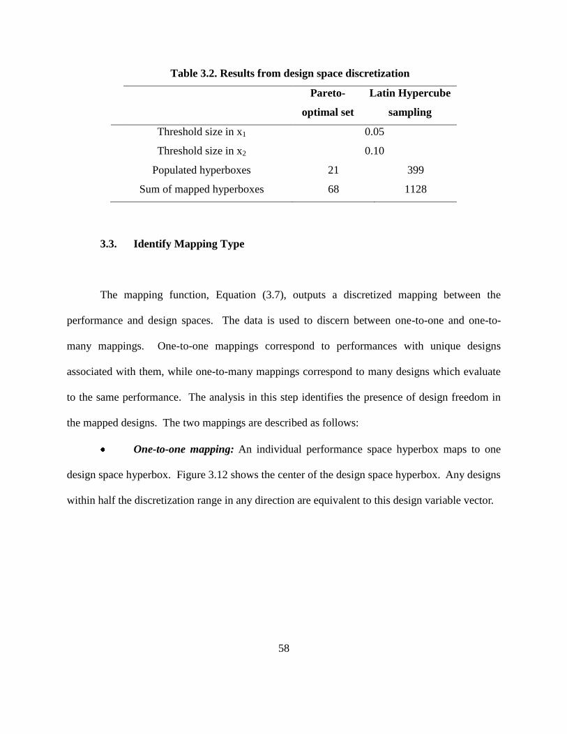
58
Table 3.2. Results from design space discretization
Pareto-
optimal set
Latin Hypercube
sampling
Threshold size in x1 0.05
Threshold size in x2 0.10
Populated hyperboxes 21 399
Sum of mapped hyperboxes 68 1128
3.3. Identify Mapping Type
The mapping function, Equation (3.7), outputs a discretized mapping between the
performance and design spaces. The data is used to discern between one-to-one and one-to-
many mappings. One-to-one mappings correspond to performances with unique designs
associated with them, while one-to-many mappings correspond to many designs which evaluate
to the same performance. The analysis in this step identifies the presence of design freedom in
the mapped designs. The two mappings are described as follows:
One-to-one mapping: An individual performance space hyperbox maps to one
design space hyperbox. Figure 3.12 shows the center of the design space hyperbox. Any designs
within half the discretization range in any direction are equivalent to this design variable vector.

59
Figure. 3.12. An example of a one-to-one mapping
One-to-many mapping: An individual performance space hyperbox maps to
multiple design space hyperboxes. Those hyperboxes can be adjacent or not. Figure 3.13 shows
how one performance space hyperbox maps to different design space hyperboxes that are
distributed throughout the design space.
Figure.3.13. An example of a one-to-many mapping
The algorithm selects some populated performance space box, . The DSBs that map
to it, , are then identified. These are the mapped design space hyperboxes.

60
The hyperbox bounds form a mapped envelope hypervolume (MEHV) in the design space which
is the integer sum of all enclosed design space hyperboxes. The reasoning for establishing
MEHVs are illustrated in Figure 3.12 and Figure 3.13. Figure 3.12 shows how a performance
maps to a small design region, confined within one design space box. The MEHV is therefore 1.
In Figure 3.13, a performance evaluates to multiple points in the design space. The mapped
designs belong to three separate design space boxes. They differ in both x1 and x2 variables.
The total area that the bounds of mapped designs encompassed is 6 hyperboxes. Figure 3.13
shows a mapping with a MEHV of 6.
The maximum distance between the bounds is calculated in Equation (3.10) and used to
evaluate the total are enclosed by the mapped hyperboxes. To calculate it, the difference in
design hyperbox bounds is computed to find the total enclosed volume, Equation (3.11).
(3.10)
(3.11)

61
The integer value of the MEHV for a given location in the performance space serves as a
metric of design freedom. One-to-one mappings are found by identifying mappings that have an
MEHV of only one design box.
Application to a simple optimization problem
Table 3.3 contains the one-to-many data obtained from the example problem. In it, every
performance space box of the Pareto-set is a one-to-many mapping. Similarly, 98% of the LHS
designs are in one-to-many mappings. Only 7 out of 325 performance hyperboxes map
identically to matching design hyperboxes. A closer inspection finds that these performances are
unique in their PSB. They are singular performances and by definition are one-to-one.
Table 3.3. Quantification of mapping types
Pareto set LHS
Performance space hyperboxes 28 325
One-to-one mappings 0 (0%) 7 (2%)
One-to-many mappings 28 (100%) 318 (98%)
The identification of one-to-many mappings is not sufficient to find regions of significant
design freedom. Some one-to-many mappings carry a higher value than others. Section 3.4,

62
describes the method that the research approach uses to find the significant one-to-many
mappings in the two sets.
3.4. Rank Mapped Hypervolumes
Each and every PSB is associated with a unique MEHV. The size of the mapped
hypervolume signifies which one-to-many mappings are associated with more significant design
freedom than others. The research approach sorts the performances by the value of the mapped
envelope design hyperboxes. The MEHVs are not weighted in the ranking process.
The preceding section used the volume of the mapped designs to differentiate between
one-to-one and one-to-many designs. In the current step, performances are selected
independently from the Pareto and LHS designs. For each set, a histogram of mapped volumes
is presented. The MEHV is computed as the fraction from the total available design space. The
reader can be reminded that the default discretization size is 5% of the range in each variable.
Therefore, the volume of the available design space is 20n, where n is the number of design
variables. Therefore, the percentage value of a MEHV is found as (3.12):
(3.12)

63
is measured as an integer by considering the number of enclosed hyperboxes,
while is the percent that an MEHV covers out of the available design space. Using the
percent volume of the mapped design space region quantifies potential amount of design space
freedom associated with each one-to-many mapping scenario. The step normalizes the
calculated MEHVs by expressing them as fractions of the overall hypervolume.
The results for both sets of evaluated designs are presented in a histogram and plotted
against each other. The ranges that are of interest are 0-1%, 1-5%, 5-10% and every consecutive
10% higher. This step is illustrated for the test example in the following section.
Application to a simple optimization problem
A histogram of the two sets of evaluated and feasible designs is shown in Figure 3.14.
The distribution of mapped volume is computed as a percentage of the design space. We can
note that the LHS set has a total of 325 elements, while the Pareto set has only 28. It is
noticeable that designs in the LHS set tend to be associated with higher MEHVs. For example,
there are 283 performance space hyperboxes that map to 1-5% of the entire design space. The
Pareto set has only 4 performance space hyperboxes that accomplish this. Further, the highest
MEHV mappings reach 9% of the total available design space.

64
Figure 3.14. Design MEHV for Pareto-optimal and LHS sets
It becomes apparent that the MEHVs associated with the LHS designs are significantly
larger than that of the optimal designs. This is explained through the fact that the LHS set
extends over the whole domain of the function while the Pareto set maps only to small design
regions. Section 3.5 identifies the location in performance space of the regions associated with
the most significant design freedom.

65
3.5. Compare Performance of Mapped Hypervolumes
The performance space hyperboxes that map to the largest design space volumes exhibit
the most significant design freedom. These performance locations are compared between the
two sets of Pareto-optimal and LHS designs. Both sets are necessary and simultaneously used in
completing this step.
By ranking performance space boxes according to their respective MEHV, it is possible
to indicate which set of designs contains candidates for further study. Good candidates map to
larger sections of the design space. For example, mapped designs that carry an MEHV of over
5% of the design space volume are more significant than 1% MEHV.
Application to simple example
Once the significant MEHV mappings are obtained, their performances are visually
identified. This step identifies the location of the PSB relative to the Pareto front. These are six
PSBs that map back with an MEHV of at least 9% of the total design volume. These
performances are presented alongside the discretized LHS set shown in Figure 3.8. For each
PSB, the average of the performances is taken and presented in Figure 3.15. The performances
with this high MEHV are located in significantly sub-optimal regions of the performance space.
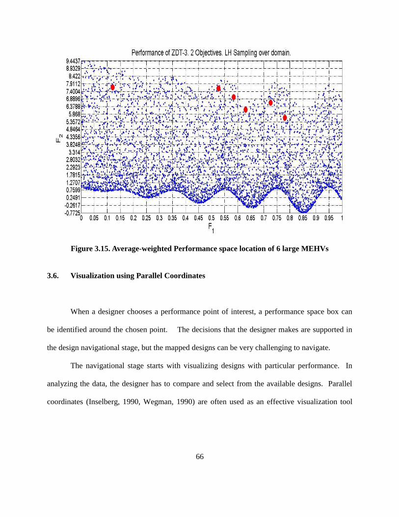
66
Figure 3.15. Average-weighted Performance space location of 6 large MEHVs
3.6. Visualization using Parallel Coordinates
When a designer chooses a performance point of interest, a performance space box can
be identified around the chosen point. The decisions that the designer makes are supported in
the design navigational stage, but the mapped designs can be very challenging to navigate.
The navigational stage starts with visualizing designs with particular performance. In
analyzing the data, the designer has to compare and select from the available designs. Parallel
coordinates (Inselberg, 1990, Wegman, 1990) are often used as an effective visualization tool

67
when communicating information of a complex nature. In this work, parallel coordinate (PC)
visualization is used to look for trends in the designs relating to a specified performance region,
and to visualize the distribution of the mapped designs. In this type of graph, each segment of
the x-axis corresponds to one of the design variables associated with the problem. The y-axis
represents the value of each design variable in the design space. Each line refers to a unique
design.
Application to a simple optimization problem
In this example problem, a PSB with center (0.125, 7.66) is selected to illustrate the
method. The performances are shown in Figure 3.16. At this level, discretization effects
become clearly visible and there are feasible performances close to the boundaries of the PSB.

68
Figure 3.16. Existing designs in the selected PSB
The design space is 2-dimensional for the example problem. It lends itself to display the
mapped designs in both 2D and PC forms. Figures 3.17 and 3.18 depict the same mapped
designs in the two different formats.

69
Figure 3.17. Mapped 2-D design space of the selected PSB
Figure 3.17 shows the data in two dimensions, x1 and x2. The designs are found across
nearly the complete range of variable x2 in two main groups, while being located over a much
smaller region of variable x1. A design that is located at (0.1502, -0.9205) shows an effect of
discretization, which is studied specifically through RQ2. This design exists in a unique DSB
because of the geometric discretization, causing the calculated MEHV to double.
Figure 3.18 shows the data in a parallel coordinates plot normalized in the range of [0,1].
The horizontal axis has x1 and x2 as its points, but the scale of the two variables is different. The
minimums are 0.1045 in x1 and -0.9267 in x2. Maximums are 0.1502 in x1 and 0.9350 in x2.
Correlations between the variables are harder to visualize unless the variable ranges are

70
normalized. For each dimension, the minimum value of a variable is plotted as 0 along the
vertical line., while the maximum value is plotted as 1. The graph easily identifies the two
groups on their dependence in x2 and the even distribution of designs along the x1 dimension.
Figure 3.18. Parallel Coordinates of the selected PSB
The introduction to PC display format ends with a note of caution. Visualization allows
the designer access to the mapped design information, but identifying possible trends might
become a significant challenge. Therefore, the thesis provides the designer with other methods
in design navigation.
71
3.7. Cluster and group data
In Section 3.6, a performance space box is selected by the user, and Parallel Coordinates
were described as a method of presenting design data. Even though the step is instructive, it
might not be possible to take a decision on design configuration solely based on it. The data
might be too complex and require too many choices. In general, people can only be expected to
make rational decisions when faced with less than 7 possible choices. This thesis aims to present
data in a structure manner that facilitates decision making. Therefore, design navigational tools
are provided in addition to the visualization in the previous section.
The analysis of the results reduces the difficulty of making decisions on the system by
lowering the number of options a designer must contend with. The mapped design ranges are
known. Nevertheless, they are not used to partition design data. The variable ranges give an
indication of the bounds but not any trends that exist within them. There can be gaps in the
design space that has no mapped designs or some of the regions are infeasible. The current
thesis pursues clustering techniques in identifying trends and partitioning designs into groups.
The methods pursued in the research approach are hierarchical clustering and K-means
clustering applied in a consecutive manner. Each application of the clustering techniques divides
the data into groups. The research approach assumes that smaller groups of designs are more
manageable. Once a small group of designs is identified with fewer than 7 elements, the
designer can easily choose a particular configuration, and the process stops, or the designer can

72
stop the process at any stage. Other information can and is given additionally. In particular,
Section 3.8 describes how the mapping information is used to generate a mapping quality metric
for each group of designs.
Both K-means and hierarchical clustering identify groups of designs that are similar to
each other and different from the rest. The research approach first applies hierarchical clustering
on the mapped designs. Hierarchical clustering is an iterative approach to prescribe every design
to some group. The first stage prescribes every design to its own group. In consequent
iterations, the two groups of designs that are most similar to each other are united. When all
designs belong to a single group, the clustering algorithm stops. The output is a tree-like
structure, called a dendrogram.
For example, three designs can be identified in Figure 3.19 as designs 1, 2 and 3. They
become the end leaf nodes in Figure 3.20. Designs 1 and 2 are closest to each other and
therefore they are united into a group branch first. The next step requires the distance between
design 3 and the group of designs 1 and 2 to be measured. The hierarchical clustering algorithm
used in this work applies the UPMGA (Unweighted Pair Group Method with Arithmetic Mean)
distance method in the linkage function in Matlab to determine the distance between groups of
designs. The method takes the average distance between each element in the two branches. In
the given example, it takes the smallest distance between designs 1 and 2 and designs 1 and 3.
Consequently, the three designs are merged together. The result is the dendrongram in Figure
3.20.

73
Figure 3.19. Sample designs
Figure 3.20. Sample dendrogram
The graph presents an access to similarity information for the designer. For example, in
an even distribution, the lowest hierarchy is formed with a balanced tree (Karypis, 2005) while
dissimilar designs will form an uneven tree. Furthermore, the horizontal length of each branch is
representative of the distance that has to be traversed to unite with the next branch. The total

74
value of the horizontal distance is the distance covered in uniting the branches. The information
can be leveraged into the design navigation process.
The calculated traversed distance is used to determine what branch to select from the
dendrogram. A fraction of the total traversed distance is calculated and used to select the level of
the dendrogram to split. It has the effect of splitting the dendrogram with vertical line, as shown
in Figure 3.21. The research approach uses 50% of the total distance to split the dendrogram in
the middle.
Figure 3.21 Dendrogram division
K-means clustering is also provided to subdivide groups of designs. It requires the
designer to choose the number of clusters that the designs are to be grouped in. K-means
clustering identifies groups of self-similar designs. The cluster partitioning aims to maximize the
distance between different clusters and minimizes distance within clusters. The research
approach performs 5 runs on every single analysis of mapped design data. It guards against

75
locally optimal clustering partitioning, which happen due to the stochastic nature of the
clustering. The multiple runs hold that the globally optimal cluster partitioning has been found.
The two clustering options, hierarchical and K-means, group designs. The user has to
choose a group of designs. The number of designs in each group is given. The design
navigation stage uses a mapping quality (MQ) metric to confirm the validity of the mapping
information. MQ evaluates multiple designs that are placed within the MEHV of some group of
designs. The fraction of the designs that evaluate to the same PSB is used to confirm the
consistency of the mapping information. The MQ information is also given to the designer in
selecting groups of designs. The validation is described in further detail in Section 3.8.
3.8. Validate Mappings
Designs that exist within the MEHV bounds of a particular PSB do not necessarily
evaluate to the same PSB. Other designs that exist inside a mapped DSB can map to any other
performance and need not evaluate back to the same PSB. There is extraneous space contained
within the mapped volume that does not necessarily evaluate to the same performance. This
becomes particularly important if a designer wants to establish if the mapping holds within the
bounds of the mapped region.
The validation process tests the mapping by placing new designs within an MEHV of
some group of designs and recording whether they evaluate back to the same PSB‘s. The design

76
space boxes that mapped designs belong to are obtained. The list of designs is generated through
a LHS. A target number of feasible designs is specified at 100 designs. Each LHS set consists
of 250 designs, which are evaluated for feasibility. Additional sets are generated until the target
number of feasible designs is reached.
The performances of the test designs can possibly be located in:
1. The same mapped PSB: indicates confirmation of the established mapping
2. A neighboring PSB to the mapped PSB: indicates sensitivity of established
mapping
3. A non-neighboring PSB to the mapped PSB: indicates a mapping outside the
established one
All three cases are possible options in a given mapping. In this work a comparison is
made only between the first and last cases. The information obtained from validating
performances can be used for two purposes. Firstly, it can be used to reinforce or rebut the
design-to-performance mapping. The step ensures that the mapping information is consistent.
Secondly, validating the mapping evaluates the possibility that the given MEHV bounds provide
a measure to place designs within the bounds to evaluate to the desired performance.
The validation process is used in conjunction with the clustering algorithms. It is applied
to a group of designs and reports the number of performances that map to the same PSB and the
total number of feasible designs sampled within the MEHV. Then the fractional percentage of
designs that map to the same PSB is computed and displayed as a percentage.

77
It allows the designer to have information on the number of designs in each cluster and
the associated MQ. From this information, the designer is expected to choose a cluster of
designs. The process is repeated if the design data remains complex.
The clustering process is stopped once a manageable data set of designs is selected: one
that has either an MQ judged high by the designer or a limited number of designs. The steps are
described as:
Step 1. Select and plot a performance space box.
Step 2. Visualize mapped designs
Step 3. If there are simple trends or designs are less than 7, stop. Otherwise, go to Step 4.
Step 4. Perform hierarchical analysis on the mapped designs
Select level of branches from the hierarchies, 50% of total distance
For each branch, provide number of designs and MQ
Step 5. The user selects a group of designs belonging to a branch.
Step 6. The group of designs is segmented using K-Means algorithm
The user decides how many segments to divide the data into
For each cluster, provide number of designs and MQ
The user decides to evaluate a new number of segments (apply Step 6 again) or to select a
cluster (continue to Step 7)
Step 7. Determine bounds and visualize designs

78
Step 8. If there are simple trends or designs are less than 7, stop. Otherwise, go to Step 4.
Figure 3.22. Navigational process diagram
Application to a simple example
The clustering and validation procedures are applied to the 9 designs that are chosen in
Section 3.6. The first step of the procedure is to apply the hierarchical analysis, which produces

79
Figure 3.23 and gives access to the dissimilarity of the designs. Referring back to Figure 3.16,
we see that the biggest difference between designs is the placement along the second coordinate,
x2. This is identified in the order that branches are merged together. The order of the node
merging identifies which designs are most similar to each other.
The current example has a small distance between designs that are either in the high or
low value of x2. Thus, the first branch merging occurs within those two groups. The 5 designs
with value of x2 > 0.9 are grouped as one branch. The 4 designs that have a value of x2 < -0.9
are grouped together. These are the blue and red branch respectively.
The height of each individual tree branch identifies how dissimilar the tree branches are.
Most of the distances are between the blue and red branches. Therefore, in Figure 3.23, the
height of the branch uniting the two is much higher compared to any other branch. The
similarity information of the design configurations is given through this type of a graph.
Figure 3.23. Hierarchical cluster analysis on mapped designs

80
The mapping quality for the identified clusters is now computed at this stage. For both
clusters, ten test designs are placed within the respective DSBs. It can be noted that members of
the red branch are associated with 2 DSB while members of the blue branch are associated with
1 DSB. The computed performances of the validating designs are presented in Figure 3.24. For
both cases, 3 out of 10 designs evaluate to the same PSB, 6 to neighboring PSBs and 1 design is
evaluated in a performance beyond that. The MQ is presented in Table 3.4. The information
from the validating mappings can be used to guide the navigational process.
Figure 3.24. validate Mappings

81
Table 3.4. Cluster Analysis using Mapping Quality Information
Branch Color Number of Mapped Designs MQ
Red 4 3/10 30%
Blue 5 3/10 30%
At this point, the designer would be asked to select a branch. We illustrate the method by
selecting the red branch that has 4 designs, which are graphed in the lower part in Figure 3.17.
At this stage, a designer can be expected to make a decision between the remaining 4 designs.
The example finishes by showing how the application of a k-means algorithm can group the data
into two clusters. The designs are shown partitioned in Figure 3.25. The means of each cluster
are shown to identify the partitions.

82
Figure 3.25. K-means application on 4 designs
3.9. Summary of Approach and Next Steps
The section is a convenient point to revisit what was established so far and list some of
the challenges that lie ahead. The section will summarize three different aspects of the chapter,
by reviewing the methodology and features in 3.9.1, discussing features that the methodology
does not addressed in 3.9.2 and listing future case studies in 3.9.3. These sections provide the
opportunity to address some key notes in the application of the research approach.
The methodology has been built on information provided in Chapters 1 and 2. In Chapter
1, the indifference threshold discretization studied in (Ferguson, 2005ab) is proposed as a

83
method to address the posed three research questions. It uses discretized performance-to-design
space mappings to analyze design freedom. The review of research efforts in Chapter 2
identified computational methods that are implemented in the research approach. The review
also demonstrated the broad spectrum of research in variability across disciplines such as ranged
sets (Chen, 2008), MGA (Gupta, 2006) and diversity-seeking MOGA (Preuss, 2009). A lack of
methods aimed at performance-to-design space mapping was also noted. The computational
methods discussed in Chapter 2 that are being used in the research approach include:
MOGAs to generate Pareto-optimal sets in sampling a design problem
LHS to fully sample the design space of a problem. This is done either to obtain
performance information across the domain (section 3.1) or to validate a mapping
(section 3.8)
Parallel Coordinates as a visualization technique in presenting complex datasets
Hierarchical and K-means clustering techniques to manage and group the designs
These techniques are successfully integrated into the research approach. The next section
addresses what functions they achieve.

84
3.9.1. Features addressed by the research approach
The research approach analyzes design freedom by implementing four main segments
shown in Figure 3.1. We will review how they are implemented in a problem to address the
three research questions.
1. Sampling designs: designs have to be sampled to represent the performance space
adequately. The two strategies in the research approach are: MOGA optimization
and LHS over the domain.
2. Obtaining PS-to-DS data: in characterizing one-to-many mappings, designs are
discretized to support the analysis and ordered pairs of performance to design data
are formed. One-to-one and one-to-many mappings are identified through this
mapping structure.
How accurate is the mapping process in representing the problem? One issue in
addressing the accuracy is the indifference threshold discretization and its effects
on the results. This question is studied as RQ2. In addressing it, the indifference
threshold for discretizing the design space is modified to yield new sets of results.
3. Rank and compare: the performances are ranked according to the bounds of their
mapped designs to identify the largest and most significant mappings. The results

85
are compared across mappings of the Pareto set and sub-optimal performances,
which addresses RQ1.
4. Navigational Tools: designs belonging to a PSB are selected and are visualized.
They are then clustered to identify segments of manageable data. The process
involves validating the mappings structure through sampling new designs within
the mapped design space, which addresses RQ3.
RQ1 studies the comparison of design freedom between Pareto-optimal and suboptimal
performances. This question is addressed through the choice in sampling in Section 3.1,
analyzed in Section 3.4, and compared in Section 3.5. RQ2 studies the effect of the application
of indifference thresholds by observing the sensitivity of different PS-to-DS data. This is
addressed by varying discretization settings in Section 3.2. RQ3 addresses the decision aspect of
the analysis in presenting the data. It is addressed through the use of navigational tools in the
research with PC visualization in Section 3.6, clustering analysis in Section 3.7 and validation
procedures in Section 3.8. The research approach addresses these various points, but the next
section discusses two points that have not been talked about yet.

86
3.9.2 Features not fully addressed
Not all features related to the research approach have been addressed fully in the chapter.
The current section briefly discusses numerical accuracy and computational time load. These
areas require further attention in analyzing the practical application of the research approach.
Concerning accuracy, how are un-sampled designs, or more importantly – un-sampled
performances - assessed? This issue in characterizing the accuracy is important for complex
problems that carry erratic properties such as non-linear or discontinuous features. Theoretically,
for a black-box problem, a performance can be obtained by a design that has not been sampled
yet. Within the thesis the issue is mitigated by including very large sampling populations to
effectively samples the design space exhaustively. This comes with a sacrifice in extending
computational time.
The research approach will require a high level of computational capacity in addressing
the complexity of the problems. In describing the computational time, it is noteworthy that most
of it is spent generating and evaluating the design population, i.e. Section 3.1. This reason
relates to complexity associated with evaluating and optimizing black-box engineering problems
(Shan, 2007, Shan, 2010) that require significant time to compute. The rest of the steps do grow
with sample size but are not as computationally intensive.

87
3.9.3 Look Ahead
The next steps will require testing the research approach on several case study problems.
The problems will aim to accommodate several different problem structures. Some sample
engineering case study problems include structural design problems and geometric parameter
choices.
Such cases studies will be covered in the following chapter, Chapter 4, which uses case
study problems to answer the research questions originally proposed in Chapter 1.

88
4. Analysis of Case Study Optimization Problems
“The purpose of computing is insight, not numbers.”
-Richard Hamming
This chapter presents the results of applying the research approach to several engineering
optimization case studies. The analysis covers three case study problems, listed in table 4.1. The
numerical results of these case study results are used to address the research questions.
The investigation computationally determines the existence of one-to-many mappings in
the case study problems. Applying the computational methods to case study problems shows
practical issues in applying the research approach. They also bring insight about the properties
of problems, in an analogy to Hamming‘s quote. The current chapter contains analysis of one-to-
many mappings which are used to determine the associated design freedom.
Table 4.1. List of tested problems
# design
variables
# objective
performances
Notes
2-bar truss 3 2 Struts supporting a weight
Motor Platform 5 2 Platform to isolate vibrations of a motor
I-Beam 4 2 Selection of an I-Beam configuration

89
The examples are sufficiently complex to provide the necessary insight toward answering
the research questions posed in Chapter 1. The case studies are chosen to examine several
different circumstances, such as a different number of design variables. The first presented case
study covers the configuration of a Bar-Truss system while supporting a weight.
4.1 Analysis of Two Bar-Truss Problem
This section presents the first multiobjective optimization problem, the analysis of a two
bar-truss. It is adapted from previous work (Azarm, 1999), and is an example of a simple
structural support. The goal of the problem is to design a system of two bar-trusses that support a
given weight, as shown in Figure 4.1. The three design variables are the height of the system, y,
and cross-sectional areas AC and BC, x1 and x2. The objectives are to minimize volume of the
system and the stress that the AC truss experiences. The desired weight that is to be supported is
set at 100 kN.
To find solutions within a reasonable range along the Pareto front, objective constraints
have been imposed. The volume of the system has to be less than 0.1 m3, described in g1. The
stress within either truss cannot exceed 100,000 kPa, which is included in g2 and g3.

90
Figure 4.1. A visualization of a 2 bar-truss problem
The problem consists of three design variables, two objective functions, and three
constraints. The problem statement for this case study is shown in Eq. (4.1).
(4.1)
Where:
(meters)

91
4.1.1 Sample Designs
The first step in the research approach is to sample the design space. Two different sets of
sampled designs are generated. The first set contains 5000 Pareto-optimal designs. They are
solved for by a genetic algorithm after 200 generations. The next sampling scheme is a Latin
Hypercube (LH), which yields 5129 unique feasible designs. The corresponding performance
space of the two sets is shown in Figure 4.2.
The two objectives ranged over different scales. The first objective, volume, is in the
range of [0, 0.1] m3. The second objective, stress, is in the range of [0, 10
5] N/m
2. The Pareto-
optimal designs identify the frontier. There are trade-offs between these two objectives in the
Pareto set. LH samples contain designs over a wide range of feasible performances.
The design space contains three design variables, allowing the data to be visualized using
3-dimensional plots. The design space of the Pareto set is shown in Figure 4.3. The Pareto
designs are confined in the range [0.0042, 0.0195] for x1, [0.00843, 0.00892] for x2, and in y
from [2.025, 3]. A further look at the figure shows that there is a portion of the designs that are
positioned around what resembles a line, (1). The rest are part of a cloud of designs, (2), that are
in the higher range of y.
The design space of the LHS is shown in Figure 4.4. It is seen that the designs do not
cover the whole design domain as one might expect. This arises from the constraints in the

92
problem that prevent designs from existing in all regions of the domain. The next section
describes how this design space is discretized.
Figure 4.2 Performances on the Pareto-optimal front and sub-optimal LH sampled designs
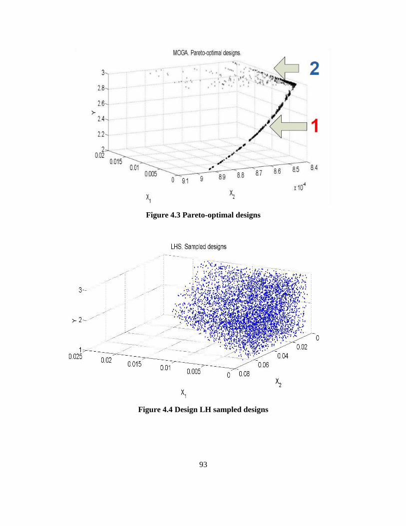
93
Figure 4.3 Pareto-optimal designs
Figure 4.4 Design LH sampled designs
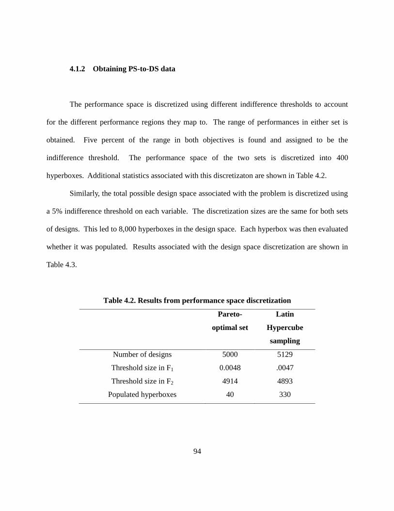
94
4.1.2 Obtaining PS-to-DS data
The performance space is discretized using different indifference thresholds to account
for the different performance regions they map to. The range of performances in either set is
obtained. Five percent of the range in both objectives is found and assigned to be the
indifference threshold. The performance space of the two sets is discretized into 400
hyperboxes. Additional statistics associated with this discretizaton are shown in Table 4.2.
Similarly, the total possible design space associated with the problem is discretized using
a 5% indifference threshold on each variable. The discretization sizes are the same for both sets
of designs. This led to 8,000 hyperboxes in the design space. Each hyperbox was then evaluated
whether it was populated. Results associated with the design space discretization are shown in
Table 4.3.
Table 4.2. Results from performance space discretization
Pareto-
optimal set
Latin
Hypercube
sampling
Number of designs 5000 5129
Threshold size in F1 0.0048 .0047
Threshold size in F2 4914 4893
Populated hyperboxes 40 330
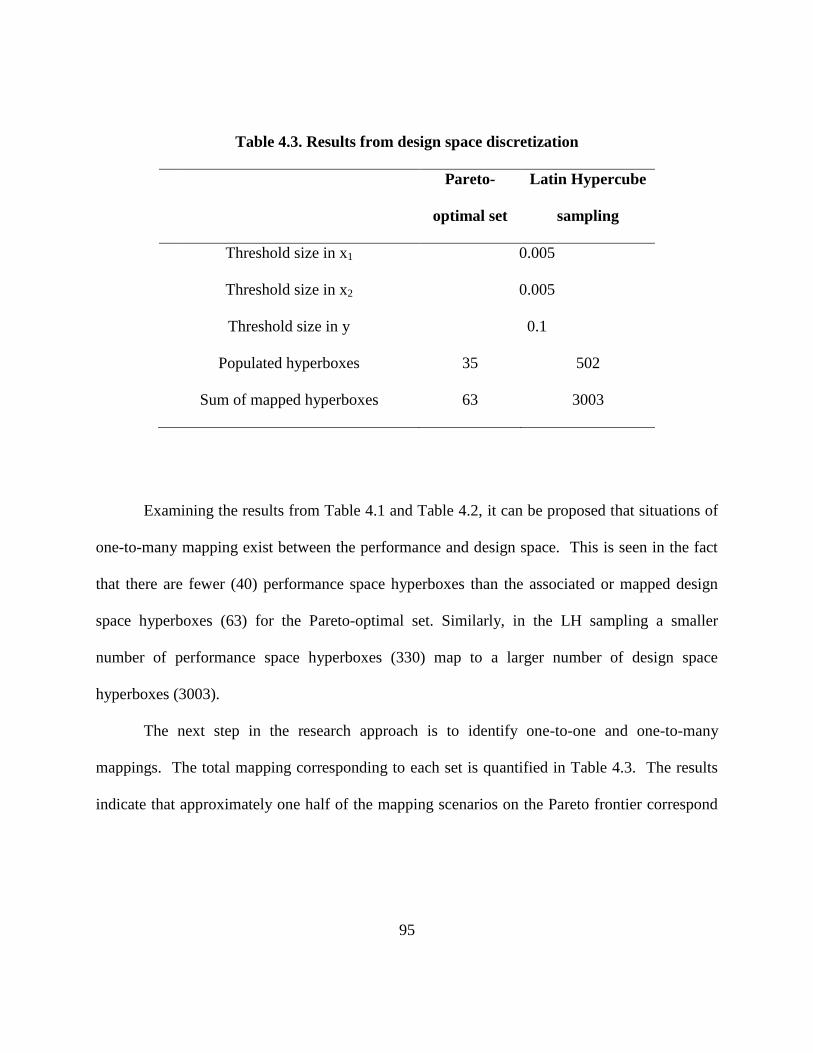
95
Table 4.3. Results from design space discretization
Pareto-
optimal set
Latin Hypercube
sampling
Threshold size in x1 0.005
Threshold size in x2 0.005
Threshold size in y 0.1
Populated hyperboxes 35 502
Sum of mapped hyperboxes 63 3003
Examining the results from Table 4.1 and Table 4.2, it can be proposed that situations of
one-to-many mapping exist between the performance and design space. This is seen in the fact
that there are fewer (40) performance space hyperboxes than the associated or mapped design
space hyperboxes (63) for the Pareto-optimal set. Similarly, in the LH sampling a smaller
number of performance space hyperboxes (330) map to a larger number of design space
hyperboxes (3003).
The next step in the research approach is to identify one-to-one and one-to-many
mappings. The total mapping corresponding to each set is quantified in Table 4.3. The results
indicate that approximately one half of the mapping scenarios on the Pareto frontier correspond

96
to one-to-many mappings, which is much higher than the one-to-many mappings of the LH
sampling.
Table 4.4. Quantification of mapping types
Pareto set LHS
Performance space hyperboxes 40 330
One-to-one mappings 21 (52.5%) 82 (24.85%)
One-to-many mappings 19 (47.5%) 248 (75.15%)
4.1.3 Rank and Compare Sets
For either set, the mapped design volume of each one-to-many mappings is computed.
The results of the mapped enclosed hypervolumes (MEHVs), a percentage of the total design
volume, are shown in Figure 4.5. The largest MEHV from the Pareto set maps to less than 1%
volume of the entire design space. This result signifies that the one-to-many mappings of the
Pareto-optimal set contain significantly less design freedom than the suboptimal set. This result
is used to address Research Question 1. The question asks what locations in the performance
space do significant one-to-many mappings occur.

97
Figure 4.5 Design MEHV for Pareto-optimal and LHS sets
Figure 4.6. Performance space location of large MEHVs

98
When plotted in the performance space, the results of the largest one-to-many mappings
from the Latin Hypercube sampling can be shown with respect to the Pareto frontier. As shown
in Figure 4.6, these mappings occur at degradation in both F1 and F2. Nevertheless, the two
objectives display different behavior for these high-design freedom regions. The high MEHV
occur at very low values of objective F2 and very ―poor‖ values of F1. However, if a designer
were interested in extra design freedom near this region of the Pareto frontier, extra design
freedom could be realized while sacrificing minimal performance.
4.1.4 Design Navigation
The designer is required to choose a desired performance for further exploration. The
Pareto set contains optimal designs that are lacking in design freedom. A theoretical
performance space box (PSB), that the designer may be interested in, has its center located at
(0.0875, 3388). The performances that lie within the same PSB and are considered equivalent
have a volume, F1, of 0.0875±0.0047 m3 and exhibit a pressure, F2, of 2446±2446. The
performances of the PSB are shown in Figure 4.7. This PSB is close to the Pareto front and
encompasses some performances that are on the front itself, these Pareto optimal points are
denoted by an ―X‖.

99
Figure 4.7. Performances associated with selected PSB
There are 208 designs that are present within the PSB. The MEHV of the PSB is 5%.
The mapped designs are presented using a parallel coordinates plot in Figure 4.8. The data is
sorted according to the third design variable, y. The values are normalized to a range between 0
and 1. The true maximum and minimum value of the axes are shown within the plot.
The plot shows how the designs spread within the three variables. No major gaps are
observed in any of the design variables. The correlations that can exist for the second variable
are less readily recognizable. For example, by following designs (1) shows that the order of
some design variables is largely reversed between the first and third variables. Some designs (2)
form parallel lines between x1 and x2, which signifies the presence of a linear relationship for

100
them. Nevertheless, presenting the design variable information of all designs leads to difficulties
in identifying every trend.
Figure 4.8. Parallel Coordinates representation of mapped designs
A designer has to make a choice on what design variable bounds to concentrate on. A
choice can be made on the specific design configuration. The information in the plot is
beneficial for designers, who can make a more informed decisions based on design variables
distribution. Yet, the number of designs and their complex behavior certainly makes the analysis
cumbersome. Trends are not always easy to identify within the parallel coordinates. Thus,

101
designs are segmented into groups to provide identifiable mappings, whose bounds can be more
informative to the designer.
To assist in the exploration phase, a sequence of hierarchical and K-means clustering is
applied. The hierarchical clustering algorithm uses the variable information in generating the
branch tree, a series of T-shaped nodes. The variable information is not directly displayed to the
designer. Instead the distances needed to unite branches together correspond to the order and
height of branches. Any branch of the tree can be accessed for further exploration.
All three variables have the same units of distance. The user can decide what weight to
put on any of the variables. For demonstrative purposes, the hierarchical clustering is performed
using Euclidian distance through the UPMGA algorithm in the variables of the mapped designs.
The algorithm combines the branch nodes that are closest by calculating the average distance
between any two elements in the two branches. The hierarchical clustering is shown in Figure
4.9. All designs are shown on the right side of the graph as the leaves of the dendrogram. The
branches form to the left. The top level node includes all of the designs.
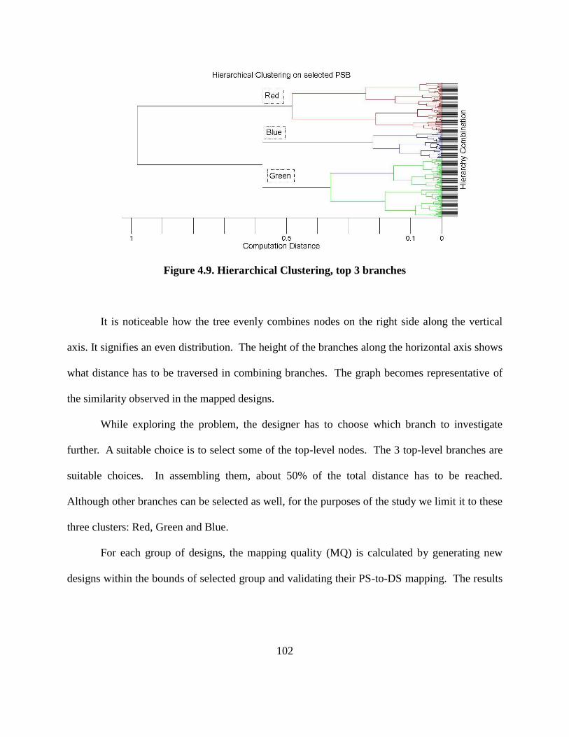
102
Figure 4.9. Hierarchical Clustering, top 3 branches
It is noticeable how the tree evenly combines nodes on the right side along the vertical
axis. It signifies an even distribution. The height of the branches along the horizontal axis shows
what distance has to be traversed in combining branches. The graph becomes representative of
the similarity observed in the mapped designs.
While exploring the problem, the designer has to choose which branch to investigate
further. A suitable choice is to select some of the top-level nodes. The 3 top-level branches are
suitable choices. In assembling them, about 50% of the total distance has to be reached.
Although other branches can be selected as well, for the purposes of the study we limit it to these
three clusters: Red, Green and Blue.
For each group of designs, the mapping quality (MQ) is calculated by generating new
designs within the bounds of selected group and validating their PS-to-DS mapping. The results

103
are shown in Table 4.5. The calculated centers of the groups are shown in Table 4.6. The user is
expected to use this data to choose one group of designs over another.
Table 4.5. Top Hierarchical Clusters Analysis on top branches
Cluster Color Number of Mapped Designs MQ
Red 75 14/152 9.0%
Blue 91 23/157 14.6%
Green 42 13/151 8.6%
Table 4.6. Centers of Top Hierarchical Clusters Analysis
X1 X2 X3
Red 0.0178 0.0082 1.2079
Blue 0.0147 0.0113 1.7853
Green 0.0132 0.0089 2.5838
It is easily noticeable that the MQ of the clusters is between 8.6% and 14.6%, which
suggests that the clusters need further refining. To illustrate the next step of refining the clusters,
the Blue branch with 91 designs is selected. The selected designs are clustered with a center of
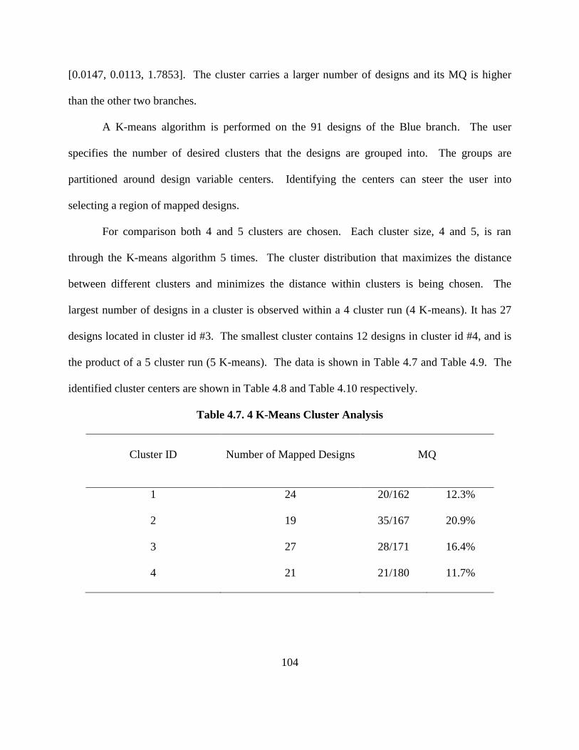
104
[0.0147, 0.0113, 1.7853]. The cluster carries a larger number of designs and its MQ is higher
than the other two branches.
A K-means algorithm is performed on the 91 designs of the Blue branch. The user
specifies the number of desired clusters that the designs are grouped into. The groups are
partitioned around design variable centers. Identifying the centers can steer the user into
selecting a region of mapped designs.
For comparison both 4 and 5 clusters are chosen. Each cluster size, 4 and 5, is ran
through the K-means algorithm 5 times. The cluster distribution that maximizes the distance
between different clusters and minimizes the distance within clusters is being chosen. The
largest number of designs in a cluster is observed within a 4 cluster run (4 K-means). It has 27
designs located in cluster id #3. The smallest cluster contains 12 designs in cluster id #4, and is
the product of a 5 cluster run (5 K-means). The data is shown in Table 4.7 and Table 4.9. The
identified cluster centers are shown in Table 4.8 and Table 4.10 respectively.
Table 4.7. 4 K-Means Cluster Analysis
Cluster ID Number of Mapped Designs MQ
1 24 20/162 12.3%
2 19 35/167 20.9%
3 27 28/171 16.4%
4 21 21/180 11.7%

105
Table 4.8 Centers of 4 K-means clusters
X1 X2 X3
Id1 0.0147 0.0119 1.6893
Id2 0.0148 0.0093 2.0552
Id3 0.0149 0.0133 1.5073
Id4 0.0146 0.0106 1.8970
Table 4.9. 5 k-Means Clusters Analysis
Cluster Color Number of Mapped Designs MQ
1 15 27/161 16.8%
2 24 26/164 15.8%
3 19 31/180 17.2%
4 12 22/185 12.0%
5 21 25/177 14.1%

106
Table 4.10 Centers of 5 K-means clusters
X1 X2 X3
Id1 0.0149 0.0133 1.5073
Id2 0.0157 0.0071 2.0838
Id3 0.0146 0.0109 1.8732
Id4 0.0147 0.0119 1.6893
Id5 0.0139 0.0113 1.9781
The user is expected to select one of the clusters from the available information. In the
presence of a user preference over a particular design space region, the cluster centers in Table
4.8 or Table 4.10 are presented. The MQ of the presented clusters ranges between 11.7% and
20.9%. If the design information or MQs were suitable, the designer could choose to stop the
process. However, to illustrate the method further, the 19 designs forming cluster id #2 in the 4
k-means are selected for further analysis.
A hierarchical analysis is performed again on the designs in accordance with the research
approach. The results are shown in Figure 4.10. This time the top 4 branches are considered.
The distance in assembling the groups is 35% of the total traversed distance. The associated
number of designs and mapping information for the top 4 branches are shown in Table 4.11.
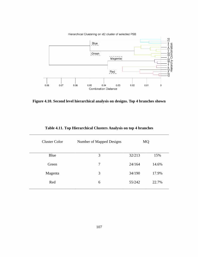
107
Figure 4.10. Second level hierarchical analysis on designs. Top 4 branches shown
Table 4.11. Top Hierarchical Clusters Analysis on top 4 branches
Cluster Color Number of Mapped Designs MQ
Blue 3 32/213 15%
Green 7 24/164 14.6%
Magenta 3 34/190 17.9%
Red 6 55/242 22.7%

108
Table 4.12. Centers of Top Hierarchical Clusters
X1 X2 Y
Blue 0.0163 0.0060 2.0775
Green 0.0146 0.0101 2.0264
Magenta 0.0140 0.0117 1.9895
Red 0.0123 0.0128 2.1266
The hierarchical clustering identifies 4 main branches. The distance traversed to combine
the designs into clusters encompasses 35% of the total distance. As we saw no substantial
increase in MQ, and with each branch containing less than 7 designs, the designer would likely
choose a single branch from which to pick the final design based on individual preferences.
The mapping quality of the 4 branches varies between 15 and 22.7%. The reader can
note that the number of feasible designs used for validation significantly increases. For example,
out of 250 validating designs for the red branch, 242 are feasible.
In making a more informed decision, the designer might want to visualize the
performances of different clusters. The performances of each branch are visualized within the
selected PSB, shown in Figure 4.11. Within Figure 4.11 the performances that belong to the red
and blue branches are indicated by suitably colored markers. Their design space is discussed in
the next paragraph.
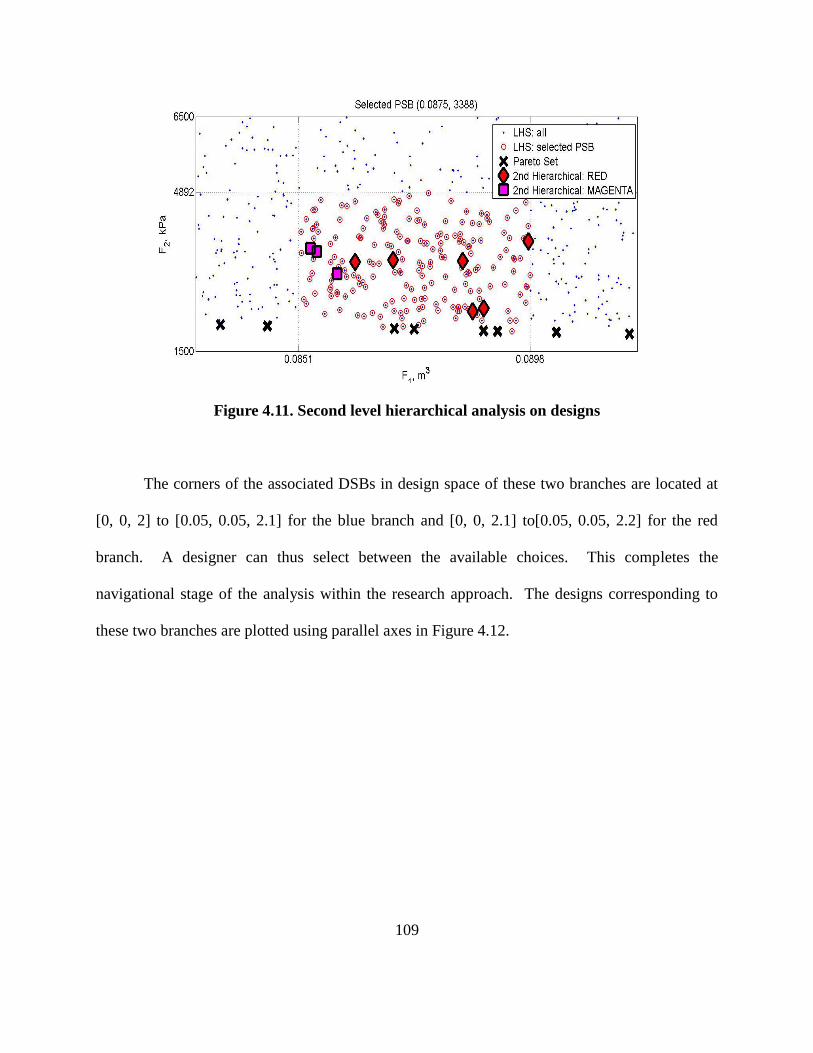
109
Figure 4.11. Second level hierarchical analysis on designs
The corners of the associated DSBs in design space of these two branches are located at
[0, 0, 2] to [0.05, 0.05, 2.1] for the blue branch and [0, 0, 2.1] to[0.05, 0.05, 2.2] for the red
branch. A designer can thus select between the available choices. This completes the
navigational stage of the analysis within the research approach. The designs corresponding to
these two branches are plotted using parallel axes in Figure 4.12.
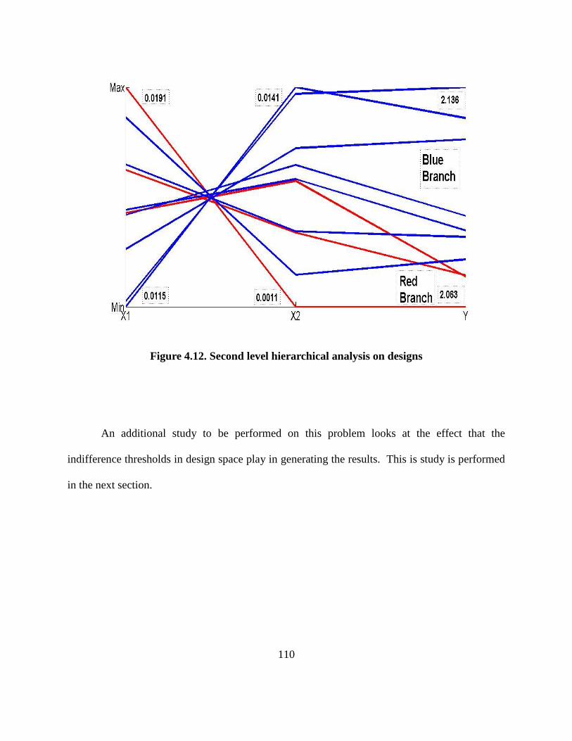
110
Figure 4.12. Second level hierarchical analysis on designs
An additional study to be performed on this problem looks at the effect that the
indifference thresholds in design space play in generating the results. This is study is performed
in the next section.

111
4.1.5 Impact of indifference thresholds
It is theorized that the indifference thresholds have the potential to steer the results in
different directions. Their effects are checked by allowing the indifference threshold in the
performance space to vary between 0.1% and 10%, while keeping the performance space
thresholds constant at 5% of PS. This has the effect of keeping the same PSB discretization and
isolating any effects to changes only in the design space. The resulting design space indifference
thresholds are shown in Table 4.13.
Table 4.13. Indifference threshold discretization
Indifference, % range X1 X2 Y
0.1% 0.0001 0.0001 0.002
0.5% 0.0005 0.0005 0.01
1% 0.001 0.001 0.02
5% 0.005 0.005 0.1
10% 0.01 0.01 0.2
Table 4.14 shows the quantity of one-to-one and one-to-many mappings as a function of
the discretization. The discretization effect changes the number of one-to-one mappings between
79 to 89. The identified 79 mappings for small discretization sizes remain one-to-one for the

112
higher discretization sizes. By observation, each of these mappings is associated with
performance that is unique within the PSB it belongs to. The discretization process places it as a
one-to-one mapping.
At higher design discretization sizes, several further mappings from the performance
space back to the design space are one-to-one mappings. 3 more mappings become one-to-one
for a 5% discretization for a total of 82. 7 additional mappings are identified as one-to-one for a
10% discretization for a total of 89. Increasing the indifference threshold size extends the size of
the design hyperboxes. Additional design configurations are indexed under a large hyperbox
instead of several smaller ones. Thus, what were classified as one-to-many mappings for smaller
discretization steps are now classified as one-to-one.
Table 4.14 also contains the sum of MEHVs and these results are shown in Figure 4.13.
Within Figure 4.13 it is shown that the largest summed MEHV value covers over 4.5 times that
of the smallest summed MEHV. These results signify that as the dicretization size increased the
number of times the DSBs are counted more than once is also increasing.
Table 4.14. Design discretization analysis
Indifference, %
range
One-to-one
mapping
One-to-many
mapping
Sum of MEHV (%
of DS volume)
0.1% 79 251 80.5%
0.5% 79 251 90.4%
1% 79 251 104.9%
5% 82 248 234.0%
10% 89 241 464.4%

113
Figure 4.13. Sum of MEHV for Two-Bar Truss
4.2 Analysis of Vibrating Motor Platform Problem
This section presents the analysis of a vibrating platform problem, which is adapted from
previous work (Azarm, 1999). The goal of the problem is to reduce the amount of vibration
transmitted by a motor. The problem assumes that higher natural frequencies of the platform
lower the transmitted vibrations. Figure 4.14 gives a representation of the problem. There is a
corresponding cost associated with different configurations where it is possible to achieve a
0.00%
50.00%
100.00%
150.00%
200.00%
250.00%
300.00%
350.00%
400.00%
450.00%
500.00%
10% 5% 1% 0.50% 0.10%% o
f D
esi
gn S
pac
e H
ype
rvo
lum
e
% indifference threshold
Sum of MEHV vs indifference thresholds

114
higher natural frequency for a higher cost. This presents an inherent trade-off between the
objective to minimize the transmitted vibrations and the cost associated with the platform.
Figure 4.14. Platform for a Vibrating Motor
The design variables associated with this problem are the thickness of the three materials
that insulate the platform (d1, d2, d3), and the length and width (L and b, respectively) of the
platform. The design objectives are to minimize cost and maximize the natural frequency. The
full optimization problem statement is shown in Eq. (4.2). The constants associated with each
material listed in Table 4.15. The platform has a constraint on the total mass (g1) and four
constraints on the thicknesses of each layer of material (g2-g5).

115
(4.2)
Where:

116
Table 4.15. Constants used in the vibrating motor problem
Property Material 1 Material 2 Material 3
ci, ($) 500 1500 800
i, ( 100 2770 7780
Ei, (GPa) 1.6 70 200
4.2.1 Sample Designs
For this problem, a genetic algorithm was used to determine the Pareto frontier shown in
Figure 4.15. After 200 generations, 9977 Pareto optimal designs were obtained. The resulting
performance space from the LHS identified 10023 unique feasible designs which are also shown
in Figure 4.15.

117
Figure 4.15. Pareto-optimal front and LHS Mapped Performance sets
4.2.2 Obtain PS-to-DS Data
The discretization is then performed with an indifference threshold of 5% of the
discovered range for each objective function. This resulted in 400 unique possible hyperboxes in
the performance space. Table 4.15 shows the associated discretization data.
Similarly, the total possible design space associated with the problem was discretized
using a 5% indifference threshold on each variable. This led to 3.2 million hyperboxes in the
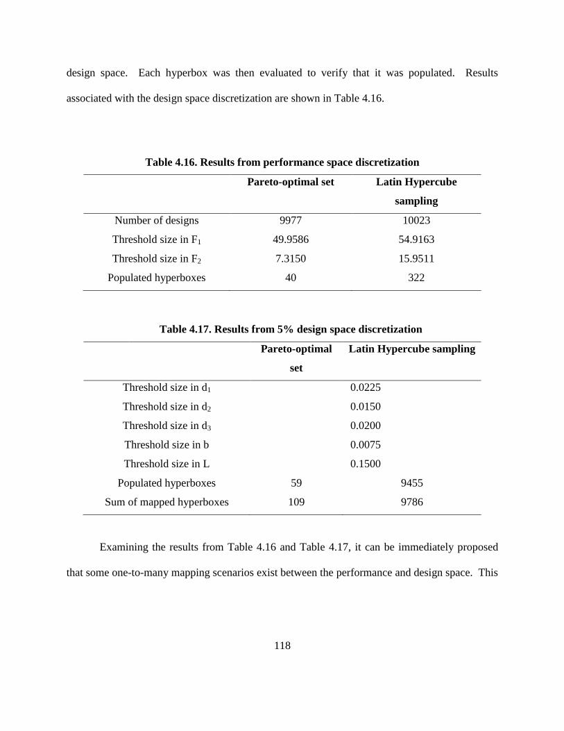
118
design space. Each hyperbox was then evaluated to verify that it was populated. Results
associated with the design space discretization are shown in Table 4.16.
Table 4.16. Results from performance space discretization
Pareto-optimal set Latin Hypercube
sampling
Number of designs 9977 10023
Threshold size in F1 49.9586 54.9163
Threshold size in F2 7.3150 15.9511
Populated hyperboxes 40 322
Table 4.17. Results from 5% design space discretization
Pareto-optimal
set
Latin Hypercube sampling
Threshold size in d1 0.0225
Threshold size in d2 0.0150
Threshold size in d3 0.0200
Threshold size in b 0.0075
Threshold size in L 0.1500
Populated hyperboxes 59 9455
Sum of mapped hyperboxes 109 9786
Examining the results from Table 4.16 and Table 4.17, it can be immediately proposed
that some one-to-many mapping scenarios exist between the performance and design space. This

119
is seen in the fact that 40 performance space hyperboxes map to 59 design space hyperboxes for
the Pareto-optimal set. Similarly, 322 performance space hyperboxes map to 9455 design space
hyperboxes for the LHS. The number of one-to-one and one-to-many mappings is quantified
and shown in Table 4.18. The results indicate that a majority of the performance space
hyperboxes correspond to one-to-many mapping scenarios. However, it is necessary to examine
what physical design ranges they signify.
Table 4.18. Quantification of mapping types
Pareto set LHS
Performance space hyperboxes 40 322
One-to-one mappings 11 (28%) 35 (11%)
One-to-many mappings 29 (72%) 287(89%)
4.2.3 Ranking and Compare Sets
Figure 4.16 examines results from the one-to-many mappings for the two sets. For each
mapping, volume of the mapped region in the design space is calculated. For this problem, the
largest MEHV calculated from the Pareto set has an area of 32 design space hyperboxes,
corresponding to only 0.001% of the entire design space region. This result implies that no
significant one-to-many mappings are detected for the Pareto-optimal set.
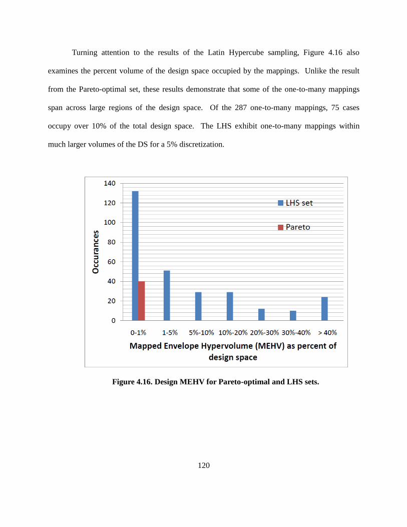
120
Turning attention to the results of the Latin Hypercube sampling, Figure 4.16 also
examines the percent volume of the design space occupied by the mappings. Unlike the result
from the Pareto-optimal set, these results demonstrate that some of the one-to-many mappings
span across large regions of the design space. Of the 287 one-to-many mappings, 75 cases
occupy over 10% of the total design space. The LHS exhibit one-to-many mappings within
much larger volumes of the DS for a 5% discretization.
Figure 4.16. Design MEHV for Pareto-optimal and LHS sets.

121
Figure 4.17 shows the centroid location of performance space hyperboxers associated
with the one-to-many mappings corresponding to over 10% of the total design space. It is seen
that they exist well within the dominated region of the performance space.
Figure 4.17. Performance space location of large MEHVs
It is significant to note that these results show the dominated regions of the performance
space may offer much greater design freedom. While multiple physical configurations are
available in this region, to reach a point on the Pareto-optimal frontier a designer is faced with a
drastically reduced choice set when specifying design configuration.

122
4.2.4 Design Navigation
To proceed with design navigation the designer needs to select a performance point of
interest. The hypothetical choice has its centroid located at (-522, 231) that maps to 30% to 40%
of the design space. Its corresponding performance points are shown in Figure 4.18.
Figure 4.18. Performances within the selected Performance Space Region
The corresponding designs are shown in Figure 4.19 using parallel coordinates. It should
be noted that the order is largely preserved in four of the design variables, d1, d2, d3, L but not in
the variable b. The order in the four variables signifies a strong correlation between these
variables in the mapped designs. The inconsistencies in b suggest the lack of direct relationship.

123
Figure 4.19. Parallel Coordinates representation of mapped designs
Relational trends are explored through an application of a hierarchical clustering on the
dataset. The resulting tree is shown in Figure 4.20. The designer selects what level of the
dendrogram to be chosen to segment the mapped designs. The highest 5 tree branches are
considered. To assemble the designs into these groups traverses half of the total distances. The
quantity of designs in these branches is shown in Table 4.19 and their centers in Table 4.20. The
validation procedure involves mapping over 100 designs.
The validating designs are constructed by placing Latin Hypercube sets of size 250
within the respective MEHV of each group of designs. Infeasible designs are discarded and a
new set of 250 designs is evaluated. The process continues until the target value of 100 feasible
designs is reached.
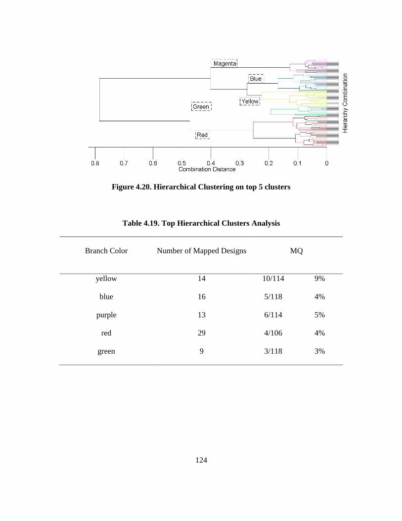
124
Figure 4.20. Hierarchical Clustering on top 5 clusters
Table 4.19. Top Hierarchical Clusters Analysis
Branch Color Number of Mapped Designs MQ
yellow 14 10/114 9%
blue 16 5/118 4%
purple 13 6/114 5%
red 29 4/106 4%
green 9 3/118 3%

125
Table 4.20. Centers of Top Hierarchical Cluster Analysis
D1 D2 D3 b L
yellow 0.4189 0.4756 0.4808 0.3937 4.4697
blue 0.3533 0.4264 0.4318 0.4015 4.2250
purple 0.3017 0.3822 0.3877 0.4189 3.9665
red 0.2157 0.3222 0.3274 0.4301 3.5897
green 0.1385 0.2568 0.2639 0.4574 3.1376
At the selected level, the branches have between 9 and 29 designs. The mapping quality
is considerably low and does not exceed 9% for any group. The MEHV of the total performance
space box is over 30% of the available design volume. The large design volume that the
validating designs are placed in can lead to low values of mapping confirmation. The
performances of the designs used for validation that are near the selected performance space
region are included next in Figures 4.21a-e.
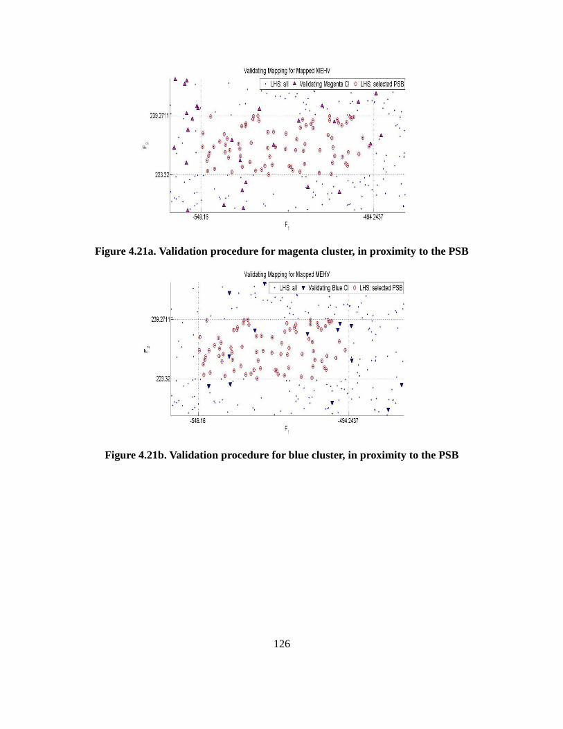
126
Figure 4.21a. Validation procedure for magenta cluster, in proximity to the PSB
Figure 4.21b. Validation procedure for blue cluster, in proximity to the PSB

127
Figure 4.21c. Validation procedure for yellow cluster, in proximity to the PSB
Figure 4.21d. Validation procedure for green cluster, in proximity to the PSB

128
Figure 4.21e. Validation procedure for red cluster, in proximity to the PSB
A large number of the validating designs have a performance that occurs outside the
selected PSB as seen in Figures 4.22a-e. The graphs depict the spread of the performances with
respect to the Pareto front as well as inform the designer how the clustered data compares with
each other.
Figure 4.22a. Validation procedure for magenta cluster, performance space

129
Figure 4.22b. Validation procedure for blue cluster, performance space
Figure 4.22c. Validation procedure for yellow cluster, performance space

130
Figure 4.22d. Validation procedure for green cluster, performance space
Figure 4.22e. Validation procedure for red cluster, performance space
The performances of the validating design within the red cluster map cover very large
areas of the performances space. Notably, the blue and red clusters contain designs that evaluate
somewhat closer to the Pareto set. Nevertheless, the yellow branch contains 14 designs with a
MQ of 13%. In the current case study, the yellow designs are explored further.

131
The 14 designs are segmented into 4 clusters through the K-means algorithm. The
resulting clusters size range between 2 and 5. Because of the small size of each individual
cluster, the dataset presented can be presented in Table 4.20.
Table 4.21. 4 K-means analysis. Design variables associated with yellow branch
ID Mapped Designs MQ
d1 d2 d3 b L In/Total
designs Percent In
1
0.434 0.494 0.503 0.378 4.701
22/119 18.5% 0.424 0.493 0.498 0.351 4.603
2
0.450 0.491 0.497 0.406 4.501
15/106 14.2%
0.443 0.490 0.497 0.400 4.528
0.416 0.491 0.497 0.363 4.506
0.422 0.493 0.495 0.365 4.452
0.392 0.463 0.472 0.370 4.507
3
0.471 0.488 0.492 0.436 4.349
29/146 19.9% 0.456 0.477 0.486 0.422 4.444
0.437 0.462 0.472 0.451 4.409
4
0.401 0.451 0.451 0.415 4.399
26/114 22.8%
0.370 0.469 0.469 0.357 4.394
0.382 0.457 0.458 0.390 4.404
0.370 0.439 0.443 0.409 4.379

132
The provision of design configurations provides the opportunity for the user to choose a
cluster of designs. The consideration of mapping quality adds additional information that can be
considered. Clusters id3 and id4 have a MQ at or above 20%. These values are higher than the
other two clusters. Therefore, they form suitable choices for a designer for the current problem
in consideration of the mapping bounds.
4.2.5 Impact of indifference thresholds
In this section we explore the impact of various indifference threshold values. Again, the
effect of the varying the indifference threshold values in the DS are explored while keeping the
PS discretization constant at 5%. Five different indifference threshold values are considered:
0.1%, 0.5%, 1%, 5%, and 10%. The associated design variable ranges with these indifference
thresholds are shown in Table 4.22.
For the Pareto-optimal set, the MEHV remained below 0.01% of the design space for any
design space indifference threshold. The design variable values for a given hyperbox having a
mean of -522 for F1 and 231 for F2 in the performance space from the LHS set is given in Table
4.23. The bounds on the mapped region in the design space can then be compared. By
comparing the sum of the mapped region in the DS, it is apparent that this PSB correlates to a
one-to-many mapping. This is further corroborated in Table 4.24, as the sum of all MEHV‘s is
almost 28 times the hypervolume of the design space. The values are graphed in Figure 4.23. It

133
can be noted that larger indifference thresholds map to larger areas of the design space. Further,
MEHV values start converging when the indifference thresholds are smaller than 5% of design
variable ranges.
Table 4.22. Discretized design variable ranges
Indifference, % range d1 d2 d3 B L
0.1 0.00045 0.0003 0.0004 0.00015 0.003
0.5 0.00225 0.0015 0.002 0.00075 0.015
1 0.0045 0.003 0.004 0.0015 0.03
5 0.0225 0.015 0.02 0.0075 0.15
10 0.045 0.03 0.04 0.015 0.3

134
Table 4.23. Mapped ranges for designs of (-522, 231) PSB
Indiff., %
range Bound
Variables ranges
d1 d2 d3 b L
0.1% Lower 0.068 0.026 0.036 0.0003 0.033
Upper 0.419 0.294 0.303 0.147 1.701
0.5% Lower 0.067 0.026 0.034 .00075 0.03
Upper 0.421 0.294 0.302 0.147 1.695
1% Lower 0.068 0.027 0.032 0 0.03
Upper 0.419 0.294 0.3 0.147 1.68
5% Lower 0.068 0.03 0.02 0 0
Upper 0.405 0.285 0.3 0.15 1.65
10% Lower 0.045 0.03 0 0 0
Upper 0.405 0.3 0.28 0.15 1.5
Table 4.24. Design discretization analysis
Indifference, %
range
One-to-one
mapping
One-to-many
mapping
Sum of MEHV (%
of DS volume)
0.1% 35 218 1982.69%
0.5% 35 218 2038.41%
1% 35 218 2110.06%
5% 35 265 2794.45%
10% 36 286 3706.73%

135
Figure 4.23. Sum of MEHVs
4.3 Analysis of I-Beam Problem
This section presents the analysis of the design of an I-Beam, adapted from previous
work (Hacker, 2002). The problem is a 4 design variable, 2 objective function problem that has
1 constraint. It is modified from the presentation in (Hacker, 2002) to include two objective
functions. The problem definition is given in Equation 4.3 and a visual representation is given
by Figures 4.24a and 4.24b. The designers are asked to make decisions regarding the structural
dimensions while minimizing cross-sectional area (F1) and minimizing vertical defelction that
0.00%
500.00%
1000.00%
1500.00%
2000.00%
2500.00%
3000.00%
3500.00%
4000.00%
10% 5% 1% 0.50% 0.10%
% o
f D
esi
gn S
pac
e H
ype
rvo
lum
e
% indifference threshold
Sum of MEHV vs indifference thresholds

136
the beam experiences (F2). The only constraint is the maximal stress that the I-Beam can
experience.
Figure 4.24a. Side view of an I-Beam
Figure 4.24b. Cross-sectional
view, showing the four variables
(4.3)

137
4.3.1 Sample Designs
For this problem, 200 generations of the genetic algorithm yielded 5000 Pareto optimal
designs. For the Latin Hypercube sampling of the design space, 10230 unique feasible designs
were identified. The results are shown in Figure 4.25.
Figure 4.25. Performance space of Pareto set and selected LHS sampling

138
4.3.2 Obtain PS-to-DS Data
Performing the discretization in the performance space resulted in 400 possible
hyperboxes. Information associated with this discretizaton is shown in Table 4.25. Similarly,
the total possible design space associated with the problem was discretized using a 5%
indifference threshold on each variable. This led to 160,000 hyperboxes in the design space.
Each hyperbox is then evaluated to test and see whether it is populated. Results associated with
the design space discretization are shown in Table 4.26.
Table 4.25. Results from performance space discretization
Pareto-optimal set Latin Hypercube
sampling
Number of designs 5000 10230
Threshold size in F1 23.10 32.8484
Threshold size in F2 0.002 0.0154
Populated hyperboxes 39 197

139
Table 4.26. Results from design space discretization
Pareto-optimal set Latin Hypercube sampling
Threshold size in x1 3.5
Threshold size in x2 2
Threshold size in x3 0.205
Threshold size in x4 0.205
Populated
hyperboxes 65 9721
Sum of mapped
hyperboxes 100 9914
Examining the results from Table 4.24 and Table 4.25, it can again be proposed that
many cases of one-to-many mapping occur in the Latin Hypercube sampling case. It is
particularly interesting to note that the Pareto-optimal set has 39 hyperboxes in the PS mapping
to 65 hyperboxes in the DS. Further investigation shows that there is a significant overlap as the
sum of the mapped hyperboxes is 100, signifying opportunities for one-to-many mappings. The
quantity of one-to-one and one-to-many mappings is presented Table 4.23. The results of which
indicate that multiple one-to-many cases exist for the Latin Hypercube sampling case and for the
Pareto-optimal set.

140
Table 4.27. Quantification of mapping types
Pareto set LHS
Performance space hyperboxes 39 197
One-to-one mappings 9 (23%) 15 (7.6%)
One-to-many mappings 30 (77%) 182 (92.4%)
4.3.3 Ranking and Compare Sets
Figure 4.26 examines the one-to-many mappings for both the Pareto-optimal set and the
results of the Latin Hypercube sampling. This result again signifies that no important one-to-
many mappings occur between the performance and design space when considering the Pareto-
optimal set. However, this example shows potential for significant one-to-many mappings when
analyzing the Latin Hypercube sampling data.

141
Figure 4.26. Design space mapped volume for LHS and the Pareto sets
When plotted in the performance space, the centroids of the five largest one-to-many
mappings from the Latin Hypercube sampling can be shown with respect to the Pareto frontier.
As shown in Figure 4.27, these centroids are located in the dominated region of the performance
space.

142
Figure 4.27. Performance space location of large MEHVs
The results in Figure 4.27 are interesting in that the there is a tradeoff pattern between the
different mapped volumes, providing some decision flexibility on which objective should see the
largest performance sacrifice.

143
4.3.4 Design Navigation
From Figure 4.27, the largest MEHV region maps to between 50% and 60% of the total
design space. The centroid of the performance space hyperbox that defines this region is located
at {345.3, 0.0229}. The performances are presented in Figure 4.28.
Figure 4.28. Selected PSB
Parallel coordinates are used in Figure 4.29 to examine the selected PSB. The designs are
sorted by design variable x3 into four distinct bands. Their relations to the other variables are
very scattered and no clear segmentation is apparent at first. It signifies the complexities

144
associating with visualizing large number of data points, over 500 designs, using parallel
coordinates. The current set of designs is a collection of dissimilar designs, so further design
navigational stages become necessary.
Figure 4.29. Mapped Designs of Selected PSB
Hierarchical clustering is performed and presented in Figure 4.30. Only the top 50
branches out of the 500 designs are presented to avoid cluttering the graph on the right side.
Therefore, the horizontal axis starts at a non-zero value. The top 7 branches are then identified
by a unique color. The corresponding data analysis is presented in Table 4.28, with the centers
presented in Table 4.29.

145
Figure 4.30. Hierarchical clustering with top 7 branches colored
Table 4.28. Top Hierarchical Clusters Analysis
Branch Color Number of Mapped Designs MQ
Pink 30 39/250 15.6%
Dark-Yellow 77 25/249 10.0%
Green 38 36/250 14.4%
Red 84 40/160 25%
Purple 102 19/228 8.3%
Light Green 69 45/248 18.1%
Blue 104 25/231 10.8%

146
Table 4.29. Centers of Top Hierarchical Clusters Analysis
X1 X2 X3 X4
Pink 55.46 34.59 1.80 3.77
Dark-Yellow 58.81 44.37 2.32 2.47
Green 65.73 36.90 2.66 2.48
Red 73.05 17.66 3.37 3.61
Purple 62.20 24.99 3.01 3.58
Light Green 74.24 43.60 2.96 1.52
Blue 72.28 30.12 2.72 2.70
The MQ of this problem is sufficiently different than the ones observed in the previous
two case studies. It is noteworthy that of the original 250 sampled designs, far fewer are found
to be infeasible. For example, there are the Pink and Green branchs that contain only feasible
validating designs. Dark-Yellow and Light-Green branches contain 248 and 249 feasible designs
out of the 250 validating designs. The low fraction of constraint-violating validating designs
shows the potential that design bounds can be identified to evaluate to specified performance.
Among the possible branch choices, the purple branch with 102 designs and MQ of 8.3%
is chosen to demonstrate the application of the research approach. Next, a K-means algorithm
segments the designs into both 5 and 10 clusters. The respective data analysis is given in Tables

147
4.30 and 4.32 with the identified cluster centers in Table 4.31 and Table 4.33. It is noticeable
that no constraint-violating validation mapping was detected for any of the clusters.
The research approach requires the designer to select a cluster in order to continue. In the
10 k-means partitioning, cluster id8 has 12 designs and an MQ value of 28.8%. Cluster id1 in
the same partitioning has a higher MQ of 34%, but it contains only 3 designs. Choosing the
cluster id1 would not allow the research approach to be demonstrated further.
Cluster id8 is selected for further explorations, because of its high MQ value and higher
number of mapped designs. Clusters from the 5 K-means were not chosen as they still contain a
significantly large number of mapped designs. The higher number of designs can illustrate the
application of hierarchical clustering within the current thesis.
Table 4.30. 5 K-means clustering
Cluster ID Number of Mapped Designs MQ
1 18 46/250 18.4%
2 25 38/249 15.3%
3 22 41/241 17.0%
4 17 38/247 15.4%
5 20 30/250 12.0%
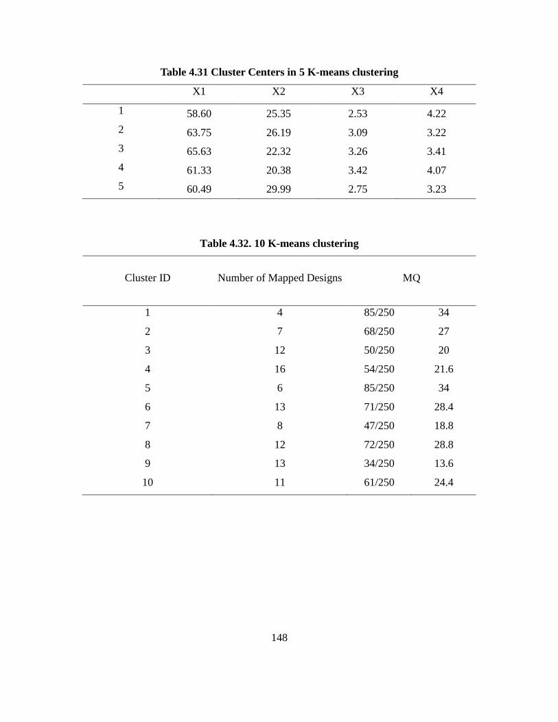
148
Table 4.31 Cluster Centers in 5 K-means clustering
X1 X2 X3 X4
1 58.60 25.35 2.53 4.22
2 63.75 26.19 3.09 3.22
3 65.63 22.32 3.26 3.41
4 61.33 20.38 3.42 4.07
5 60.49 29.99 2.75 3.23
Table 4.32. 10 K-means clustering
Cluster ID Number of Mapped Designs MQ
1 4 85/250 34
2 7 68/250 27
3 12 50/250 20
4 16 54/250 21.6
5 6 85/250 34
6 13 71/250 28.4
7 8 47/250 18.8
8 12 72/250 28.8
9 13 34/250 13.6
10 11 61/250 24.4

149
Table 4.33. Cluster centers in 10 K-means clustering
X1 X2 X3 X4
1 55.49 26.76 2.27 4.42
2 60.53 18.75 3.45 4.61
3 65.39 24.54 3.74 2.42
4 61.96 25.40 3.02 3.50
5 58.25 29.11 2.74 3.51
6 62.38 21.78 3.21 3.82
7 64.74 28.06 2.84 3.20
8 66.24 21.45 3.07 3.84
9 61.46 30.58 2.79 3.05
10 59.18 24.76 2.46 4.38
The designs that belong to cluster id8 in the 10 k-means cluster are examined further.
Hierarchical clustering is performed on the 12 design configurations. The results are shown in
Figure 4.31. The highest two branches correspond to 90% of the covered distance. This
corresponds to existing variability between the higher-level clusters as opposed to the lower-
level nodes. The associated mapping analysis is presented in Table 4.34.
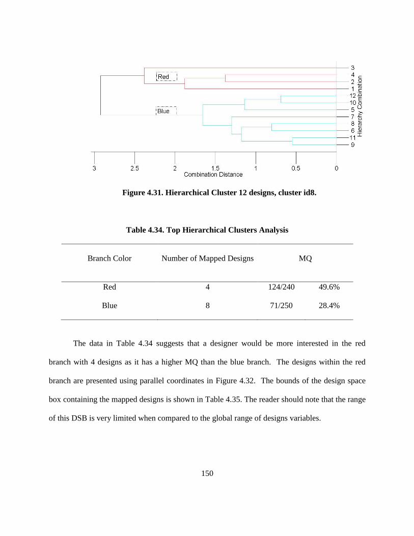
150
Figure 4.31. Hierarchical Cluster 12 designs, cluster id8.
Table 4.34. Top Hierarchical Clusters Analysis
Branch Color Number of Mapped Designs MQ
Red 4 124/240 49.6%
Blue 8 71/250 28.4%
The data in Table 4.34 suggests that a designer would be more interested in the red
branch with 4 designs as it has a higher MQ than the blue branch. The designs within the red
branch are presented using parallel coordinates in Figure 4.32. The bounds of the design space
box containing the mapped designs is shown in Table 4.35. The reader should note that the range
of this DSB is very limited when compared to the global range of designs variables.

151
Figure 4.32. Designs in the branches of the hierarchical analysis
Table 4.35. Mapped Design Hyperbox Bounds Ranges
Bounds X1 X2 X3 X4
Lower 66.5 20 2.05 2.255
Higher 70 24 3.895 4.920
4.3.5 Impact of indifference thresholds
As before, a study on the indifference threshold discretization is conducted. The results
are shown in Table 4.35 for the design space discretization sizes. The corresponding mappings
are shown in Table 4.36. The results are plotted in Figure 4.33.

152
An interesting result for this problem is that the summation of the mapped design space
for the Pareto-optimal set corresponds to only 1% of the total volume. For the Latin Hypercube
sampling dataset, the combined sum of mapped regions of the design space amounts to over 13
times the total design space volume. This result suggests that using an encompassing hyperbox
provides significant extraneous regions of the design space when one-to-many mappings are
encountered.
Furthermore, the same 12 DSBs are encountered for all of the one-to-one mappings. It is
a feature of the exhaustive sampling performed for this problem and the problem‘s modality.
Table 4.36. Discretized design variable ranges
Indifference, % range X1 X2 X3 X4
0.1 0.07 0.04 0.0041 0.0041
0.5 0.35 0.2 0.0205 0.0205
1 0.7 0.4 0.041 0.041
5 3.5 2 0.205 0.205
10 7 4 0.41 0.41

153
Table 4.37. Design discretization analysis
Indifference, %
range
One-to-one
mapping
One-to-many
mapping
Sum of MEHV (%
of DS volume)
0.1% 15 182 906.0
0.5% 15 182 935.0%
1% 15 182 973.7%
5% 15 182 1315.1%
10% 15 182 2018.3%
Figure 4.33. Sum of MEHVs.
0.00%
500.00%
1000.00%
1500.00%
2000.00%
2500.00%
10% 5% 1% 0.50% 0.10%% o
f D
esi
gn S
pac
e H
ype
rvo
lum
e
% indifference threshold
Sum of MEHV vs indifference thresholds

154
5. Overview and Discussion
This chapter provides a summary of results, revisits the research questions, and provides
sources of future work. In Chapter 1, the motivation behind identifying regions of design
freedom was established, and three research questions were posed. In Chapter 2, the necessary
computational background and design concepts were discussed. These topics included
multiobjective optimization, genetic algorithms, and Latin Hypercube sampling. Research
efforts across disciplines whose goals are related to design freedom were also presented.
The research approach of this thesis was then presented in Chapter 3. This approach
contains computational steps that comprise four parts: 1) sample designs, 2) obtain performance-
to-design space information, 3) rank and compare mapping information, and 4) design
navigation. A simple case study example is also included to demonstrate the implementation of
the proposed approach. Additionally, the numerical results of three case study problems are
reported in Chapter 4.
The current chapter is split into five sections. Section 5.1 presents answers to the
research questions posed in Chapter 1, while Section 5.2 contains the contributions of the
research approach used in this work. Sources of future work are described in Section 5.3,
Section 5.4 discusses limitations of this method, and Section 5.5 has the final overview.

155
5.1 Revisiting the Research Questions
This section addresses the three research questions originally posed in Chapter 1. In this
work, design freedom has been defined as similar performance being achieved by dissimilar
designs. The definition has been aimed particularly in a mass customization context where
customers pick a performance and chose among designs having the desired functionality. The
research assertion is that one-to-many mappings signify design freedom and support product
configurators for use in a mass customization environment.
The research approach is based on computational methods. It identifies and analyzes
performance regions with high values of design freedom. Designs are sampled through either
Latin Hypercube Sampling or a multiobjective Genetic Algorithm. For each sampling, the
performance and design space are discretized. The design freedom associated with each
performance is computed, and performances with significant-design freedom are identified. In
analyzing the results, the designer is given the choice of guided navigation for the mapped
designs of a particular performance.
5.1.1 Research Answer of RQ1
The first research question posed in Chapter 1 asks the designer to evaluate the presence
of design freedom through one-to-many mappings. The question is restated again is:
156
Research Question 1: Do one-to-many mappings located on the Pareto frontier show
significantly less design freedom than those in sub-optimal regions?
Multiple one-to-many mappings were observed for both Pareto-optimal and sub-optimal
regions. The significance of each performance is quantified by the hypervolume that mapped
designs occupy. Pareto-optimal and sub-optimal regions are compared for the presence of
significant one-to-many mappings. The location of the mappings in performance space
addresses the first research question. The research answer is that:
Research Answer 1: The significant one-to-many mappings were observed in the sub-
optimal and not Pareto-optimal performance regions
While both samplings contained multiple one-to-many mappings, the significant one-to-
many mappings were observed only in sub-optimal regions of the performance space. Case
study problems not shown in this work but completed during the course of this research indicate
similar trends.
Optimality is frequently confined within small regions of the design space in various
optimization problems. Cases where these regions are discontinuous allow for greater design
freedom. Relatively small performance degradation with respect to the Pareto front can
potentially lead to a notable increase in design freedom. Comparison between results from the

157
different case study problems indicates that this feature is specific to each individual problem.
Performance regions of design freedom were encountered in two-bar truss problem close to the
Pareto frontier.
5.1.2 Research Answer of RQ2
The use of indifference thresholds has the effect of discretizing both design and
performance spaces into hyperbox regions. The construction of the mappings requires the
designer to explicitly choose an indifference threshold size. In order to investigate the effect of
the choice, the second research question posed in Chapter 1 was:
Research Question 2: How is the sensitivity of design freedom with respect to indifference
thresholds characterized?
Design discretization sizes are applied in the design space. The default indifference
threshold is 5% of the domain of each variable. In addressing the research question, the
indifference threshold is varied between 0.1% and 10%. Mapped design space volume is filled
in with extraneous space between designs. The change in indifference thresholds affects the
amount of extraneous space filled within the bounds. The sum of the mapped volume over the

158
available dominated performances is computed for each indifference threshold. The sensitivity
of results in the case study problems gives the following research answer:
Research Answer 2: Regions of result sensitivity were observed with an increase in space
discretization size at and over 5%
The extraneous space that is between the bounds of mapped performances rises with the
size of the indifference threshold. It is signified by the sum of the mapped volumes over all
performances. The steepest growth that is shown as the threshold sizes range from 5% to 10%.
This indicates an underlying sensitivity that the effect of the indifference threshold has on the
results.
The designer has to balance the indifference threshold to identify possible one-to-many
mappings. A designer studying a problem can use special knowledge and intuition in defining
the thresholds. The designer makes the choice how to specify the thresholds that consequently
affect the design freedom. The analyzed design freedom is a function of these input values.
The quantified design freedom exhibited sensitivity in the circumstances of high
indifference thresholds. The results will vary depending on the discretization size. The designer
is interested in differentiating between one-to-one and one-to-many mappings and might not
want to choose too small of an indifference threshold.

159
It is therefore beneficial for a designer to exploring the indifference a problem in
quantifying design freedom. In the absence of further information, a starting point for
exploration can be suggested as 5%.
5.1.3 Research Answer of RQ3
A problem is sampled and design freedom analyzed in its performance space. The
designer has to choose the performance region of interest. The numerous mapped designs that
evaluate to the equivalent performances pose a complex decision for the designer. Making a
decision which designs to choose among the mapped designs is a complex decision. The
exploration stage inspires the third research question.
Research Question 3: Can methods be implemented to explore design choices, in order to
identify mapping trends and visualize the data?
The question addresses the issue of managing the complexity of design navigation. The
current thesis explores tools in exploring the mappings and navigating the designs. Four
methods are integrated together within the thesis in alleviating the complexity in making
decisions on design configurations. Their features are described as:

160
1. Parallel coordinates: the technique displays multidimensional data. It allows the
designer to visually identify trends.
2. Mapping quality: it evaluates the mapping consistency of mapped designs. It is
used to confirm the effectiveness of using a particular mapping structure.
3. Hierarchical clustering: it uses the dissimilarity between designs into constructing
hierarchical trees of design configurations. The consideration of associated
dissimilarity potentially impacts decisions with regards to design freedom.
4. K-means clustering: the process segments mapped designs into groups. It
identifies physically relevant and similar design configurations.
The variety of techniques provides a set of choices for the designer. The different
objective that the techniques cover can be leveraged when analyzing a performance. The
application of the methods in the case study problems supports the resulting research answer:
Research Answer 3: Implemented methods in design navigation stage identify trends in
mapped designs and visualize data to support decision-making process
The bounds of the mapped designs are given to the designer. Visualization of
multidimensional mapped designs is provided through the use of parallel coordinates. It supports

161
the visual identification of trends. Nevertheless, it becomes harder for a designer to make a
decision in the case of large data segments.
The mapping validation evaluates the consistency of designs that reside within the
mapped bounds. The quality of the mappings for larger bounds is shown not to be sufficiently
high to support a design choice. Therefore, designs are segmented into smaller groups. The
thesis provided the choice for hierarchical and K-means clustering.
The two clustering techniques show promising results in partitioning the designs into
similar designs. The dendrodram graphs produced by hierarchical clustering informed the
designer of the similarity in the data. The K-means clustering segmented the designs into a
number of groups chosen by the designer. The mapping quality of groups was measured to
inform the designer of the mapping consistency.
The partitioning of designs into smaller groups is associated with an increase in the
mapping quality. The process identifies design hyperbox regions that map in to the chosen
performance. This allows the designer to consider the bounds of the group of designs or to make
a selection among a selected group of designs.
The design navigation shows how the applied method alleviates the overlying complexity
in identifying these regions. Further work in visualization and design navigation can add an
additional value to the process. It becomes one of the sources of future work, discussed in the
next section.

162
5.2 Sources for Future Studies
The current thesis raises multiple directions that can be pursued in future studies. Some
examples are listed below:
1. The further study of complex problems
In practice, design problems become more complex and have discontinious
elements in their objective functions. The study can be extended to problems
such as race car configuration (Ferguson, 2005a), the design of angle-grinders
(Azarm, 2009) or other large-scale engineered systems.
2. Relating performance degradation to observed increase in design freedom
The relationship between the performance degradation from the Pareto-optimal
performances to significant regions of design freedom has not been directly
quantified. Generation of alternative designs close to the Pareto set can be
implemented. The data can evaluate how slight performance degradation relates
to design freedom.
3. Minimize computational time
The increase in computing power allows much more complex problems to be
tackled. Nevertheless, the large number of evaluations necessary for the
construction of the mapping structure consumes a potentially large amount of

163
time. Computational methods such as parallel evaluation of designs or cloud
computing become valuable options in order to alleviate the issues.
This list can be used as a starting point for possible sources of future work. The
information that can be used from the discretized mappings can be developed further. There are
series of possible other avenues, ranging from theoretical developments, marketing
investigations and research into design navigation.
5.3 Limitations
The use of sampled designs raises the question of unsampled designs – namely, can an
unsampled design significantly affect the analysis? This case is especially important for
discontinuous and non-linear problems. It has yet to be shown how to ensure that sufficient
sampling of a problem has been achieved. Further, the method can require a significant number
of evaluations. When the number of design evaluations has to be increased significantly, the
method will have to be extended to handle the larger evaluation load in creating the sampling set.
164
5.4 Concluding Remarks
The possible computational capacity allows the evaluation of multiple designs. They
lead to various paths of achieving desired performances. An important remark is that simulation
techniques allow the analysis of competing designs. The decisions can therefore extend beyond
pure performance evaluation to decisions made depending on design configurations. The
availability of design navigation is a powerful enabling technique in engineering design.
The important conclusion from the thesis is that it shows that suboptimal performances
achieve greater design freedom than Pareto-optimal designs. The method captures an inherent
value of suboptimal performances. One-to-many mappings quantify design freedom, which can
influence a designer beyond the consideration of optimality.

165
REFERENCES
Allen, J. K., C. Seepersad, H. Choi, and F. Mistree (2006). ―Robust design for multiscale and
multidisciplinary applications.‖ Journal of Mechanical Design 128(4), 832–843.
Arenbeck, H., S. Missoum, A. Basudhar, and P. Nikravesh (2010). ―Reliability-based optimal
design and tolerancing for multibody systems using explicit design space decomposition.‖
Journal of Mechanical Design 132(2), 021010+.
Azarm, S., Reynolds, B. J., and Narayanan, S., (1999). ―Comparison of Two Multiobjective
Optimization Techniques with and within Genetic Algorithms,‖ 1999 ASME Design Engineering
Technical Conferences, Las Vegas, NV, DETC99/DAC-8584.
Azarm, S., B. Besharati, L. Luo, and P. K. Kannan (2006). Multi-objective single product robust
optimization: An integrated design and marketing approach. Journal of Mechanical Design
128(4), 884–892.
Azarm, S. and S. Gunawan (2005). A feasibility robust optimization method using sensitivity
region concept. Journal of Mechanical Design 127(5), 858–865.
Azarm, S. and M. Li (2008). Multiobjective collaborative robust optimization with interval
uncertainty and interdisciplinary uncertainty propagation. Journal of Mechanical Design 130(8),
081402+.
Azarm, S., M. Li, and N. Williams (2009). Interval uncertainty reduction and single-disciplinary
sensitivity analysis with multi-objective optimization. Journal of Mechanical Design
131(3),031007+.
Azarm, S. and A. K. Maddulapalli (2006). Product design selection with preference and attribute
variability for an implicit value function. Journal of Mechanical Design 128(5), 1027–1037.

166
Azarm, S. and Z. P. Mourelatos (2006). Robust and reliability-based design. Journal of
Mechanical Design 128(4), 829–831.
Azarm, S., N. Williams, and P. K. Kannan (2008). Engineering product design optimization for
retail channel acceptance. Journal of Mechanical Design 130(6), 061402+.
Bertsche, B. and V. D. Ingenieure (2008). ―Reliability in automotive and mechanical
engineering: determination of component and system reliability.‖ Springer.
Benini,E and Toffolo, A. (2003, June). Genetic diversity as an objective in multi-objective
evolutionary algorithms. Evolutionary Computation 11(2), 151–167.
Brockhoff, D. and E. Zitzler (2007, September). ―Improving hypervolume-based multiobjective
evolutionary algorithms by using objective reduction methods.‖ In 2007 IEEE Congress on
Evolutionary Computation, pp. 2086–2093. IEEE.
Cacuci, D. G., M. Ionescu-Bujor, and I. M. Navon (2003). ―Sensitivity and uncertainty analysis.‖
Boca Raton: Chapman & Hall/CRC Press.Chang, S., E. Brilljr, and L. Dhopkins (1983).
Modeling to generate alternatives: A fuzzy approach. Fuzzy Sets and Systems 9(1-3), 137–151.
Chen, T. Y. and H. C. Chen (2009). ―Mixeddiscrete structural optimization using a rank-niche
evolution strategy.‖ Engineering Optimization 41(1), 39–58.
Chen, W., H. Lui, M. J. Scott, and K. Qureshi (2007). ―Determination of ranged sets of design
specifications by incorporating design-space heterogeneity.‖ Engineering Optimization 40(11),
1011–1029.
Chen, W., T. W. Simpson, J. K. Allen, and F. Mistree (1999). ―Satisfying ranged sets of design
requirements using design capability indices as metrics.‖ Engineering Optimization 31(5), 615–
619.

167
Chen, W. and S. Lee (2009). ―A comparative study of uncertainty propagation methods for
black-box-type problems.‖ Structural and Multidisciplinary Optimization 37(3), 239–253.
Chu, X.-Z., L. Gao, H.-B. Qiu, W.-D. Li, and X.-Y. Shao (2010). ―An expert system using rough
sets theory and self-organizing maps to design space exploration of complex products.‖ Expert
Systems with Applications.
de Weck, O. L. and M. B. Jones (2006). ―Isoperformance: Analysis and design of complex
systems with desired outcomes.‖ Syst. Engin. 9(1), 45–61.
Deb, K. (2001). ―Multi-Objective Optimization Using Evolutionary Algorithms.‖ John Wiley &
Sons.
Devendorf, E. and K. Lewis (2008). ―Planning on mistakes: An approach to incorporate error
checking into the design process.‖ ASME Conference Proceedings 2008(43253), 273–284.
Eberhart, R. C., Y. Shi, and J. Kennedy (2001, April). ―Swarm Intelligence‖ (The Morgan
Kaufmann Series in Evolutionary Computation) (1st ed.). Morgan Kaufmann.
Lewis, K. E. and J.Eddy (2002). ―Visualization of multidimensional design and optimization
data using cloud visualization.‖ ASME Conference Proceedings 2002(36223), 899–908.
Ehrgott, M., C. M. Fonseca, X. Gandibleux, J.-K. Hao, and M. Sevaux (Eds.) (2009).
―Evolutionary Multi-Criterion Optimization‖, 5th International Conference, EMO 2009, Nantes,
France, April 7-10, 2009. Proceedings, Volume 5467 of Lecture Notes in Computer Science.
Springer.
Eysenck, M.W. and M.T. Keane (2005, June). Cognitive psychology : a student's handbook.
Psychology Press.

168
Ferguson, S., A. Gurnani, J. Donndelinger, and K. Lewis (2005). ―Feasibility assessment in
preliminary design using pareto sets.‖ In DETC2005.
Ferguson,S., J. Donndelinger and K. Lewis (2006). ―Exploring mass trade-offs in preliminary
vehicle design using pareto sets.‖ In Multidisciplinary Analysis and Optimization Conference.
Ferguson, S., E. Kasprzak, and K. Lewis (2009, August). ―Designing a family of reconfigurable
vehicles using multilevel multidisciplinary design optimization.‖ Structural and
Multidisciplinary Optimization 39(2), 171–186.
Ferguson, S. and K. Lewis (2004). ―Effective development of flexible systems in
multidisciplinary optimization.‖ Volume 2004-4309.
Foster, G. and S. Ferguson (2010, September). ―Exploring the impact of distance metrics on
alternative generation in a multiobjective problem.‖ In AIAA/ISSMO Multidisciplinary Analysis
Optimization Conference. AIAA.
Frecker, M ,X.Zhang, X., T. W. Simpson, and G. Lesieutre (2009). Supporting trade space
exploration of multi-dimensional data with interactive multi-scale nested clustering and
aggregation. In DETC.
Goh, C. and K. Tan (2007). ―Evolving the tradeoffs between pareto-optimality and robustness in
multi-objective evolutionary algorithms.‖ In S. Yang, Y.-S. Ong, and Y. Jin (Eds.), Evolutionary
Computation in Dynamic and Uncertain Environments, Volume 51, Chapter 20, pp. 457–478.
Berlin, Heidelberg: Springer Berlin Heidelberg.
Gupta, A. and Kripakaran (2006). ―Mga – a mathematical approach to generate design
alternatives.‖ In Intelligent Computing in Engineering and Architecture, pp. 408–415.
Hacker, K. and K. Lewis (2002). Robust design through the use of a hybrid genetic algorithm.
DETC.

169
Hacker, K., J. Eddy, and K. Lewis (2001). ―Tuning a hybrid optimization algorithm by
determining the modality of the design space.‖ In DETC.
Hohm, T. and E. Zitzler (2009). ―A multiobjective evolutionary algorithm for numerical
parameter space characterization of reaction diffusion systems.‖ In V. Kadirkamanathan, G.
Sanguinetti, M. Girolami, M. Niranjan, and J. Noirel (Eds.), Pattern Recognition in
Bioinformatics, Volume 5780, Chapter 15, pp. 162–174. Berlin, Heidelberg: Springer Berlin
Heidelberg.
Jones, D. R., M. Schonlau, and W. J. Welch (1998, December). Efficient global optimization of
expensive black-box functions. Journal of Global Optimization 13(4), 455–492–492.
Kasprzak, E. M. and K. E. Lewis (2001, October). Pareto analysis in multiobjective otimization
using the collinearity theorem and scaling method. Structural and Multidisciplinary Optimization
22(3), 208–218.
Karypis, G and Y Zhao (2005). Data clustering in life sciences — karypis lab. Molecular
Biotechnology 31(1), 55–80.
Kaufmann, M., D. Zenkert, and P. Wennhage (2010, March). ―Integrated cost/weight
optimization of aircraft structures.‖ Structural and Multidisciplinary Optimization 41(2), 325–
334.
Kim, I. and O. de Weck (2006, February). ―Adaptive weighted sum method for multiobjective
optimization: a new method for pareto front generation.‖ Structural and Multidisciplinary
Optimization 31(2), 105–116.
Kuczera, R. C. and Z. P. Mourelatos (2009). ―On estimating the reliability of multiple failure
region problems using approximate metamodels.‖ Journal of Mechanical Design 131(12),
121003+.
170
Lay, S. R. (2000). Analysis: with an introduction to proof. Prentice Hall.
Li, M., S. Azarm, and A. Boyars (2006). A new deterministic approach using sensitivity region
measures for multi-objective robust and feasibility robust design optimization. Journal of
Mechanical Design 128(4), 874–883.
Lu, S. and H. M. Kim (2009). ―A regularized inexact penalty decomposition algorithm for
multidisciplinary design optimization problem with complementarity constraints.‖ In DETC.
Machwe, A. T. and I. C. Parmee (2007). ―Multi-objective analysis of a component-based
representation within an interactive evolutionary design system.‖ Engineering Optimization
39(5), 591–613.
Malak, R. (2008). ―Using parameterized efficient sets to model alternatives for systems design
decisions‖ - Georgia Tech‘s Institutional Repository. Ph. D. thesis, Georgia Tech.
Malak, R. J., J. M. Aughenbaugh, and C. J. J. Paredis (2009). ―Multi-attribute utility analysis in
set-based conceptual design.‖ Computer-Aided Design 41(3), 214–227.
Marler, R. T. and J. S. Arora (2004, April). Survey of multi-objective optimization methods for
engineering. Structural and Multidisciplinary Optimization 26(6), 369–395.
Marin, V. E., D. A. Romero, and J. A. Rincon (2009). ―A comparison of metamodel-assisted pre-
screening criteria for multi-objective genetic algorithms.‖ In DETC.
Mattson, C. A., A. A. Mullur, and A. Messac (2004). Smart pareto filter: obtaining a minimal
representation of multiobjective design space. Engineering Optimization 36(6), 721–740.
McDougall, R. and S. Nokleby (2009). ―On the application of multi-objective parallel
asynchronous particle swarm optimization to engineering design problems.‖ In DETC.

171
Messac, A. W. Chen, A. Sahai, and G. J. Sundararaj (2000). ―Exploration of the effectiveness of
physical programming in robust design.‖ Journal of Mechanical Design 122(2), 155–163.
Messac, A., M. P. Martinez, and T. W. Simpson (2002). ―Introduction of a product family
penalty function using physical programming.‖ Journal of Mechanical Design 124(2), 164–172.
Mistree, F., T. W. Simpson, T. W., D. Rosen, J. K. Allen (1998). Metrics for assessing design
freedom and information certainty in the early stages of design. Journal of Mechanical Design
120(4), 628–635.
Mistree, F. and B. Bras and (1995). ―A compromise decision support problem for axiomatic and
robust design.‖ Journal of Mechanical Design 117(1), 10–19.
Naone, E. (2010, February). Making sense of mountains of data. Technology Review.
Oberoi, S. and S. Finger (2009). ―Interactive design navigational tools.‖ In DETC 2009-87706.
ASME.
Olewnik, A., T. Brauen, S. Ferguson, and K. Lewis (2004). ―A framework for flexible systems
and its implementation in multiattribute decision making.‖ Journal of Mechanical Design 126(3),
412–419.
Pahl, G., W. Beitz, J. Feldhusen, and K. H. Grote (2007). ―Engineering Design: A Systematic
Approach‖ (3rd ed.). Springer.
Papalambros, P. Y. (2010, March). Design intent. Journal of Mechanical Design 132.
.
Park, G.-J. (2007). Analytic Methods for Design Practice. Springer.

172
Parmee, I. C. and C. L. Simons (2007). A cross-disciplinary technology transfer for search-based
evolutionary computing: from engineering design to software engineering design. Engineering
Optimization 39(5), 631–648.
Picheny, V., D. Ginsbourger, O. Roustant, R. T. Haftka, and N. H. Kim (2010). Adaptive designs
of experiments for accurate approximation of a target region. Journal of Mechanical Design
132(7), 071008+.
Piller, F. T. and M. Muller (2004). A new marketing approach to mass customisation.
International Journal of Computer Integrated Manufacturing 17(7), 583–593.
Preuss, M., B. Naujoks, and G. Rudolph (2006). Pareto set and emoa behavior for simple
multimodal multiobjective functions. In Parallel Problem Solving from Nature - PPSN IX, pp.
513–522.
Preuss, M.,O. Shir, M., B. Naujoks, and M. Emmerich (2009). Enhancing decision space
diversity in evolutionary multiobjective algorithms. In M. Ehrgott, C. M. Fonseca, X.
Gandibleux, J.-K. Hao, and M. Sevaux (Eds.), Evolutionary Multi-Criterion Optimization,
Volume 5467, Chapter 12, pp. 95–109. Berlin, Heidelberg: Springer Berlin Heidelberg.
Ranjan, P., D. Bingham, and G. Michailidis (2008, November). Sequential experiment design for
contour estimation from complex computer codes. Technometrics 50(4), 527–541.
Rudolph, G. and M. Preuss (2009). A multiobjective approach for finding equivalent inverse
images of pareto-optimal objective vectors. In C. Coello Coello, P. P. Bonissone, and Y. Jin
(Eds.), 2009 IEEE Symposium on Computational Intelligence in Multicriteria Decision-Making
(IEEE MCDM 2009), Piscataway (NJ), pp. 74–79. IEEE Press.
Saltelli, A., M. Ratto, T. Andres, F. Campolongo, J. Cariboni, D. Gatelli, M. Saisana, and S.
Tarantola (2008). ―Global Sensitivity Analysis.‖ The Primer. John Wiley & Sons, Ltd.

173
Shan, S. and G. G. Wang (2004). Space exploration and global optimization for computationally
intensive design problems: a rough set based approach. Structural and Multidisciplinary
Optimization 28(6), 427–441.
Shan, S. and G. Wang (2010,). ―Survey of modeling and optimization strategies to solve high-
dimensional design problems with computationally-expensive black-box functions.‖ Structural
and Multidisciplinary Optimization 41(2), 219–241.
Shneiderman, B. (2007, December). Creativity support tools: accelerating discovery and
innovation. Commun. ACM 50(12), 20–32.
Shneiderman, B. and J. Seo (2006). ―Knowledge discovery in high-dimensional data: Case
studies and a user survey for the rank-by-feature framework.‖ IEEE Transactions on
Visualization and Computer Graphics 12(3), 311–322.
Simpson, T. W., S. M.Clarke, and J. H. Griebsch(2005), ―Analysis of support vector regression
for approximation of complex engineering analyses.‖ Journal of Mechanical Design 127(6),
1077–1087.
Simpson, T. W., D. B. Spencer, M. A. Yukish, and G. Stump (2008). Visual steering commands
and test problems to support research in trade space exploration. In ISSMO Multidisciplinary
Analysis and Optimization Conference. AIAA.
Sobek, D., A. Ward, and J. Liker (1999). Toyota‘s principles of set-based concurrent
engineering. Sloan Management Review 40(2), 67–83.
Tappeta, R. V. and J. E. Renaud (1997). Multiobjective collaborative optimization. Journal of
Mechanical Design 119(3), 403–411.
Tenne, Y. and S. Armfield (2007). A memetic algorithm using a trust-region derivative-free
optimization with quadratic modelling for optimization of expensive and noisy black-box

174
functions. In S. Yang, Y.-S. Ong, and Y. Jin (Eds.), Evolutionary Computation in Dynamic and
Uncertain Environments, Volume 51, Chapter 17, pp. 389–415. Berlin, Heidelberg: Springer
Berlin Heidelberg.
Tumer, K. and A. Agogino (2007). Evolving multi rover systems in dynamic and noisy
environments. In S. Yang, Y.-S. Ong, and Y. Jin (Eds.), Evolutionary Computation in Dynamic
and Uncertain Environments, Volume 51, Chapter 16, pp. 371–387. Berlin, Heidelberg: Springer
Berlin Heidelberg.
Ulrich, T., D. Brockhoff, and E. Zitzler (2008). Pattern identification in pareto-set
approximations. In GECCO ‘08: Proceedings of the 10th annual conference on Genetic and
evolutionary computation, New York, NY, USA, pp. 737–744. ACM.
Vadde, S., J. K. Allen, and F. Mistree (1994). The bayesian compromise decision support
problem for multilevel design involving uncertainty. Journal of Mechanical Design 116(2), 388–
395.
Vanderplaats, G. N. (2007). Multidiscipline Design Optimization. Vanderplaats Research and
Development, Inc.
Vazquez, E. and J. Bect (2009). A sequential bayesian algorithm to estimate a probability of
failure. 15th IFAC Symposium on System Identification, Saint-Malo
Wang, H., N. H. Kim, and Y. J. Kim (2006). Safety envelope for load tolerance and its
application to fatigue reliability design. Journal of Mechanical Design 128(4), 919–927.
Wu, J. and S. Azarm, S. (2001). Metrics for quality assessment of a multiobjective design
optimization solution set. Journal of Mechanical Design 123(1), 18–25.
Yin, X. and W. Chen (2008). A hierarchical statistical sensitivity analysis method for complex
engineering systems design. Journal of Mechanical Design 130(7), 071402+.

175
Zitzler, E., K. Deb, and L. Thiele (2000). Comparison of multiobjective evolutionary algorithms:
Empirical results. Evolutionary Computation 8, 173–195.

176
Appendix

177
Appendix A: GA Toolbox Configuration File
# Input file for the GA Toolbox. Multiobj4/ZDT3
# Author: Peter Simov
# Date: May,2010
#
#
# GA type: SGA or NSGA
#
NSGA
#
# Number of decision variables
#
2
#
# For each decision variable, enter:
# decision variable type, Lower bound, Upper bound
# Decision variable type can be double or int
#

178
double 0 1
double -1 1
#
# Objectives:
# Number of objectives
# For each objective enter the optimization type: Max or Min
#
2
Min
Min
#
# Constraints:
# Number of constraints
# For each constraint enter a penalty weight
#
0
#
# General parameters: If these parameters are not entered default
# values will be chosen. However you must enter

179
# "default" in the place of the parameter.
# [population size]
# [maximum generations]
# [replace proportion]
#
5000
200
0.5
#
# Niching (for maintaining multiple solutions)
# To use default setting type "default"
# Usage: Niching type, [parameter(s)...]
# Valid Niching types and optional parameters are:
# NoNiching
# Sharing [niching radius] [scaling factor]
# RTS [Window size]
# DeterministicCrowding
#
# When using NSGA, it must be NoNiching (OFF).
#
NoNiching

180
#
# Selection
# Usage: Selection type, [parameter(s)...]
# To use the default setting type "default"
#
# Valid selection types and optional parameters are:
# RouletteWheel
# SUS
# TournamentWOR [tournament size]
# TournamentWR [tournament size]
# Truncation [# copies]
#
# When using NSGA, it can be neither SUS nor RouletteWheel.
#
TournamentWOR 2
#
# Crossover
# Crossover probability
# To use the default setting type "default"
#

181
# Usage: Crossover type, [parameter(s)...]
# To use the default crossover method type "default"
# Valid crossover types and optional parameters are
# OnePoint
# TwoPoint
# Uniform [genewise swap probability]
# SBX [genewise swap probability][order of the polynomial]
#
0.9
SBX 0.5 10
#
# Mutation
# Mutation probability
# To use the default setting type "default"
#
# Usage: Mutation type, [parameter(s)...]
# Valid mutation types and the optional parameters are:
# Selective
# Polynomial [order of the polynomial]
# Genewise [sigma for gene #1][sigma for gene #2]...[sigma for gene #ell]
#

182
0.1
Polynomial 20
#
# Scaling method
# To use the default setting type "default"
#
# Usage: Scaling method, [parameter(s)...]
# Valid scaling methods and optional parameters are:
# NoScaling
# Ranking
# SigmaScaling [scaling parameter]
#
NoScaling
#
# Constraint-handling method
# To use the default setting type "default"
#
# Usage: Constraint handling method, [parameters(s)...]
# Valid constraint handling methods and optional parameters are
# NoConstraints

183
# Tournament
# Penalty [Linear|Quadratic]
#
NoConstraints
#
# Local search method
# To use the default setting type "default"
#
# Usage: localSearchMethod, [maxLocalTolerance], [maxLocalEvaluations],
# [initialLocalPenaltyParameter], [localUpdateParameter],
# [lamarckianProbability], [localSearchProbability]
#
# Valid local search methods are: NoLocalSearch and SimplexSearch
#
# For example, SimplexSearch 0.001000 20 0.500000 2.000000 0.000000 0.000000
NoLocalSearch
#
# Stopping criteria
# To use the default setting type "default"
#

184
# Number of stopping criterias
#
# If the number is greater than zero
# Number of generation window
# Stopping criterion, Criterion parameter
#
# Valid stopping criterias and the associated parameters are
# NoOfEvaluations, Maximum number of function evaluations
# FitnessVariance, Minimum fitness variance
# AverageFitness, Maximum value
# AverageObjective, Max/Min value
# ChangeInBestFitness, Minimum change
# ChangeInAvgFitness, Minimum change
# ChangeInFitnessVar, Minimum change
# ChangeInBestObjective, Minimum change
# ChangeInAvgObjective, Minimum change
# NoOfFronts (NSGA only), Minimum number
# NoOfGuysInFirstFront (NSGA only), Minimum number
# ChangeInNoOfFronts (NSGA only), Minimum change
# BestFitness (SGA with NoNiching only), Maximum value
#
0

185
#
# Load the initial population from a file or not
# To use the default setting type "default"
#
# Usage: Load population (0|1)
#
# For example, if you want random initialization type 0
# On the other and if you want to load the initial population from a
# file, type
# 1 <population file name> [0|1]
#
# Valid options for "Load population" are 0/1
# If you type "1" you must specify the name of the file to load the
# population from. The second optional parameter which indicates
# whether to evaluate the individuals of the loaded population or not.
0
# Save the evaluated individuals to a file
#
# To use default setting type "default".
#

186
# Here by default all evaluated individuals are stored and you will be
# asked for a file name later when you run the executable.
#
# Usage: Save population (0|1)
# For example, if you don't want to save the evaluated solutions type 0
# On the other and if you want to save the evaluated solutions
# 1 <save file name>
#
# Note that the evaluated solutions will be appended to the file.
#
# Valid options for "Save population" are 0/1
# If you type "1" you must specify the name of the file to save the
# population to.
1 evaluatedSolutions_multiobj4_2.txt