aalborg universitet physical layer parameter and algorithm...
TRANSCRIPT

Aalborg Universitet
Physical Layer Parameter and Algorithm Study in a Downlink OFDM-LTE Context
Rom, Christian
Publication date:2008
Document VersionPublisher's PDF, also known as Version of record
Link to publication from Aalborg University
Citation for published version (APA):Rom, C. (2008). Physical Layer Parameter and Algorithm Study in a Downlink OFDM-LTE Context. Departmentof Electronic Systems, Aalborg University.
General rightsCopyright and moral rights for the publications made accessible in the public portal are retained by the authors and/or other copyright ownersand it is a condition of accessing publications that users recognise and abide by the legal requirements associated with these rights.
? Users may download and print one copy of any publication from the public portal for the purpose of private study or research. ? You may not further distribute the material or use it for any profit-making activity or commercial gain ? You may freely distribute the URL identifying the publication in the public portal ?
Take down policyIf you believe that this document breaches copyright please contact us at [email protected] providing details, and we will remove access tothe work immediately and investigate your claim.
Downloaded from vbn.aau.dk on: august 08, 2018
Physical Layer Parameter andAlgorithm Study in a Downlink
OFDM-LTE Context
Christian Rom
A dissertation accepted by the Faculty of Engineering,
Science and Medicine of Aalborg University in fulfilment of
the requirements for the degree of Doctor of Philosophy.
Radio Access Technology section
Department of Electronic Systems
Aalborg University
Denmark
June 2008

Dedicated tomy beloved parents.

c©Christian Rom 2008
ISSN 0908-1224
ISBN 87-92078-78-8

Physical Layer Parameter and Algorithm Study
in a Downlink OFDM-LTE Context
Christian Rom
Accepted for the degree of Doctor of Philosophy
June 2008
Abstract
This Ph.D. is made in cooperation between Infineon Technologies Denmark, and
the Radio Access Technologies (RATE) section at the Department of Electronic
Systems. The development of the LTE standard has been based on new increased
requirements, with high demands for spectral efficiency, reduced system and termi-
nal complexity, cost and power consumption. This leads to investigate the duality
between physical layer parameter and baseband receiver algorithm design in this
Ph.D. thesis. More specifically the work has been focused on physical layer pa-
rameters and baseband algorithms design for OFDM in a downlink LTE context.
The study is based on an accurate baseband matrix-vector model of the received
signal. The model is useful to separate two different cases: a Cyclic Prefix (CP)
length larger than the radio channel maximum excess delay, and a CP shorter than
the maximum excess delay. The LTE baseband parameter design has been investi-
gated with an emphasis on optimal CP length. In the case of a CP length larger
than the maximum excess delay, an in-depth survey of linear Pilot Assisted Chan-
nel Estimation (PACE) algorithms has been conducted leading to the development
of a novel unified modeling for fair comparison of PACE algorithms. The effect of
virtual subcarriers as well as non-sample-spaced channel model is studied, showing
that DFT based algorithms are only useful at low SNR values, but are subject to
the leakage effect as the SNR increases (above 10dB). A clear dependency between
a-priori information considered at the receiver and performance is established. To
avoid the leakage effect only two algorithm types are useful: robust wiener filters

v
and interpolators using exact channel tap delay knowledge. A methodology for pilot
pattern design has lead to a pilot scheme proposal for the downlink of LTE. Results
are characterized without error correction coding in terms of uncoded BER, SINR
and mean squared error estimates, and with error correction coding in terms of
packet error rate and spectral efficiency. In the case of a CP length shorter than
the maximum excess delay, interference cancelation techniques were investigated to
cope with insufficient guard interval length, leading to the development of a novel
algorithm: the Low-Complex-Interference-Cancelation (LCIC) algorithm.
Overall in this work, it has been shown that signal processing effort spent in
the UE can increase the system spectral efficiency. If effort is spent on accurate
tap delay estimation, much lower frequency direction pilot spacing can be used. In
the same manner, the CP length can be reduced by using the proposed interference
cancelation schemes.
Keywords: OFDM, LTE, Cyclic Prefix, Pilot Scheme, Channel Estimation, In-
terference Cancelation.
June 18, 2008
Dansk resume
Dette Ph.D. er blevet udført i samarbejde med et lokalt firma, Infineon Technolo-
gies Denmark, og RATE sectionen i Institut for Elektroniske Systemer. Ønsket om
at have et mobilt bredband som kan suportere stadige forøget data transmissions
hastigheder samt øger spektral effektiviteten, har styret telekommunications stan-
darder fra GSM, UMTS, HSPA og nu til den kommende LTE. Denne Ph.D. tese
har fokuseret pa det fysiske lags parameter design samt baseband algoritme design
for OFDM i en downlink LTE kontekst. Studiet er baseret pa en njagtig baseband
matrix-vektor modelering af det modtaget signal. Parameter design er blevet un-
dersøgt med speciel fokus pa den optimale CP længde og pilot skema design. En
dybdegaende nutidig undersøgelse af kanal estimerings algoritmer er blevet udført
og munder ud i udviklingen af en ny entydig modellering for at kunne udføre en
fair sammenligning af kanal estimerings algoritmer. En klar afhængighed mellem
a-prori information antaget i modtageren og performance er etableret. Til slut, un-
dersøges interferens ophævelses tekniker for at kunne klare korte CP længder. En
ny algoritme er udviklet: LCIC. Overordnet set, er det blevet pavist at digital sig-
nal processering i UE kan øge system spektral effektivitet. Hvis processerings kraft
bliver brugt pa nøjagtig estimering af tap forsinkelser kan der bruges væsentlig min-
dre pilot frekvens mellememrum. Pa samme made, kan CP længden reduceres ved
at udføre smart interferens ophævelses tekniker.
Declaration
The work in this thesis is based on research carried out at the ”Institut for Elek-
troniske Systemer” at Aalborg University, in the Radio Access Technology (RATE)
section, Denmark. No part of this thesis has been submitted elsewhere for any other
degree or qualification. Some of the the work carried out is based on joint research.
The parts with joint effort will be specified out. A large Link Level matlab based
simulator was developed together with my fellow Ph.D. students: Na Wei, Akhilesh
Pokhariyal and Basuki E. Priyanto. The work conducted in channel estimation has
been largely carried out in cooperation with my former student and now colleague
Carles Navarro Manchon, same goes for the work on interference cancelation carried
out with my other former student and now colleague Guillaume Monghal.
Copyright c© 2008 by Christian Rom.
“The copyright of this thesis rests with the author. No quotations from it should be
published without the author’s prior written consent and information derived from
it should be acknowledged”.
vii
Acknowledgements
The work for the present thesis has been conducted under the supervision of associate
Professor Troels Bundgaard Sørensen. I would like to thank Professor Sørensen for
all the time spent and patience during this work. In the same manner, I would
like to thank my co-supervisor Professor Preben Mogensen, for his clever guidance
and straightforward technical wisdom. A special thanks to my other co-supervisor
Dr. Benny Vejlgaard, who always believed in me and made the cooperation with
Infineon Technologies run smoothly.
I want to express my gratitude towards some employees of Infineon Technologies
in Munich, and of IKT-Duisburg with whom I had the pleasure of working during
my 6 month stay abroad, namely: Dr. Jens Berkmann, Dr. Christian Drewes, Dr.
Bertram Gunzelmann, Dr. Cecillia Carbonelli, Dr. Stefan Fechtel, Dr. Alfonso
Troya, Professor Peter Jung, Dr. Guido Bruck, Dr. Tobias Scholand, Christoph
Spiegel and Zijan Bai.
I would like to especially thank my colleague and paper co-author Carles Navarro
Manchon for all the time we have spent together. Muchas gracias por todo tio,
siempre seras un gran amigo. Also, the warmest thanks to my other colleague and
paper co-author Guillaume Monghal. Merci mon cher ami, pour ta sympatie et ton
attention pendant se temps a Aalborg.
The author would also like to thank colleagues at the RATE section, namely
Assistant Professor Luc Deneire, Na Wei, Akhilesh Pokhariyal, Basuki E. Priyanto
and Lisbeth Schiønning Larsen.
Finally I thank my parents Svend and Tove Rom for all their moral support from
the distance. Tak til jer mine kære forældre for jeres gode rad og talmodighed.
viii
Notation and Abbreviations
Scalar Symbols
αtti: number of OFDM symbols in a TTI block
αceb: number of OFDM symbols in a channel estimation block
Nt: Number of CIR taps
Ng: number of samples for the CP
Nu: number of Used (active) subcarriers
Nfft: number of input and output samples of the transmitter FFT
Nofdm: number of samples per OFDM symbol including the CP
Np: number of pilots subcarriers
No,slot: number of OFDM symbols per slot
No,sec: number of OFDM symbols per second
αf : the number of OFDM symbols in a frame
Pceb number of pilots in 1 CEB
kmod: number of bits per data symbol
s: outer iteration index
S: maximal number of outer iterations
t: continuous time index
f : continuous frequency index
n: sample index
∆f : subcarrier spacing
k: subcarrier index
m: OFDM symbol index
Tg: Cyclic Prefix duration
ix
x
Tmed: maximum Excess Delay duration
Tu: duration of basic OFDM symbol without CP
Tofdm: OFDM symbol duration with CP
Tf : LTE Frame duration
Tslot: LTE Slot duration
Ts: receiver sample time
fk: baseband frequency of subcarrier k
Fs: baseband sampling frequency
lm,p[n]: nth sample of the time varying CIR at the mth transmitted OFDM symbol
V : velocity
g(t, τ) : continuous complex baseband CIR
αi(t): time variant attenuation factor of the ith CIR tap
τi(t) : time variant ith CIR tap propagation delay
θi(t) : time variant phase value of the ith CIR tap
fc : Tx signal carrier frequency
rg : ACF of CIR
rh : Spaced-time spaced-frequency correlation function
Sh : Fourier Transform of the CIR ACF
tcor : Coherence time
(∆f)c : Coherence bandwidth
BD : Doppler spread
fd : Doppler frequency
C: bias function for SINR evaluation
Np: number of pilots in 1 OFDM symbol with pilot information
Ne: number of Eigenvalues
Ltotal: performance loss in dB differing from the optimal receiver
Lpilot: performance loss in dB due to pilot overhead
Lalgo: performance loss in dB due to channel estimation error
Lici: performance loss in dB due to ICI from doppler distortion
bi: LCIC matrix-row band index
I: LCIC band Length
June 18, 2008
xi
Vectors
b: data bits
d: transmitted data symbol
s: conceptual transmitted time OFDM signal
s: baseband transmitted OFDM signal
sm: mth baseband transmitted OFDM signal
ψk: orthogonality function of subcarrier k
r: received signal on TTI level
rm: received signal on OFDM symbol level
w: AWGN on TTI level
wm: AWGN on OFDM symbol level
g: sample spaced CIR vector
gm: sample spaced CIR for the mth OFDM symbol
h: channel transfer function vector
hm: channel transfer function vector for the mth OFDM symbol
g : non sample spaced CIR vector d: data symbol vector on TTI level
dm: data symbol vector for the mth OFDM symbol
z: received signal after FFT on TTI level
zm: received signal after FFT on OFDM symbol level
y: received signal after channel CTF matching on TTI level
ym: received signal after channel CTF matching on OFDM symbol level
gm: CIR vector assumed constant during transmission of 1 OFDM symbol
Matrices
Ψ: IDFT and CP matrix on TTI level
Ψm: IDFT and CP matrix for the mth OFDM symbol
H: channel convolution matrix on TTI level
June 18, 2008

xii
H0: channel convolution matrix on OFDM symbol level generating ICI
H1: channel convolution matrix on OFDM symbol level generating ISI
Rxx: autocorrelation matrix of vector x
C0m: ISI matrix
C1m: CTF + ICI matrix
F: DFT matrix
I: identity matrix
C : Wiener filter matrix
D: transmitted symbols matrix
June 18, 2008

xiii
Mathematical Notation
The notations used throughout this paper are:
∀ : for all
∈ : membership
(·)∗ : complex conjugate
(·)H : hermitian transpose of a matrix or vector
| · | : absolute value
⌈·⌉ : lowest integer value which is not smaller
than the argument
⌊·⌋ : rounds the argument to the nearest integer
greater than or equal to the argument
tr{·} : trace operator
diag{x} : diagonal matrix with elements of x in the diagonal
E{·} : expectation operator
F{·} : Fourier transform operator
csgn{·} : symbol hard decision operator
⇐⇒ : equivalence
≫ : much larger that
≪ : much lower that
x[k] : the kth element of a vector x
X[n, k] : the nth row and kth column element of
matrix X
x : estimate of x
N : natural numbers
Z : integer numbers
C : complex numbers
Bold upper-case letters are used for matrices and bold lower-case letters are used
for vectors.
June 18, 2008
xiv
Abbreviations
3GPP : third Generation Partnership Project
ACF : Auto-Correlation Function of the CIR
ACK : Acknowledgement
ARQ : Automatic Repeat-request
AWGN : Additive White Gaussian Noise
BS : Base Station
BER : Bit Error Rate
BLAST : Bell Labs Layered Space-Time
CP : Cyclic Prefix
CMAC : Complex Multiply Accumulate
CEB : Channel Estimation Block
CIR : Channel Impulse Response
CRC : Cyclic Redundancy Check
CQI : Channel Quality Indicator
DDA : Decision Directed Algorithm
DDCE : Decision Directed Channel Estimation
DL : Downlink
DTX : Discontinuous packet Transmission
DVB-H : Digital Video Broadcast Handheld
DVB-T : Digital Video Broadcast Terrestrial
ECR : Effective Code Rate
EDGE : Enhanced Data Rates for GSM Evolution
EGC : Equal Gain Combining
FDD : Frequency Division Duplex
FDLA : Frequency Division Link Adaptation
FDM : Frequency Division Multiplexing
FEC : Forward Error Correcting Codes
FFT : Fast Fourier Transform
GSM : Global System for Mobile communications
June 18, 2008
xv
GPRS : General Packet Radio Service
HARQ : Hybrid Automatic Repeat-request
HSDPA : High-Speed Downlink Packet Access
HSUPA : High-Speed Uplink Packet Access
ICI : Inter Carrier Interference
IC : Interference Cancelation
IR : Incremental Redundancy
ISI : Inter Symbol Interference
ISDB : Integrated Services Digital Broadcasting
LCIC : Low Complexity Interference Cancelation (scheme)
LE : Linear Equalizer
LS : Least Squares
LTE : Long Term Evolution
MCS : Modulation and Coding Set
MBMS : Multimedia Broadcast Messaging Service
MBWA : Mobile Broadband Wireless Access
MED : Maximum Excess Delay
MMSE : Minimum Mean Square Error
MRC : Maximum Ratio Combining
MS : Mobile Station
NACK : Negative Acknowledgement
OFDM : Orthogonal Frequency Division Multiplexing
OFDMA : Orthogonal Frequency Division Multiplexing Access
PSAM : Pilot Symbol-Assisted Modulation
PACE : Pilot Assisted Channel Estimation
PDP : Power Delay Profile
QAM : Quadrature Amplitude Modulation
QPSK : Quadrature Phase Shift Keying
RATE : Radio Access Technologies (section at AAU)
June 18, 2008
xvi
RAT : Radio Access Technology
RRM : Radio Resource Management
RU : Resource Unit
SAW : Stop and Wait
SEL : Spectral Efficiency Loss
SISO : Single Input Single Output
SFC : Space Frequency Coding
SFN : Single Frequency Network
STE : Single Tap Equalizer
TDD : Time Division Duplex
TFRC : Transport Format and Resource Combination
T-DMB : Terrestrial Digital Multimedia Broadcasting
UMTS : Universal Mobile Telecommunications System
UTRA : UMTS Terrestrial Radio Access
UE : User Equipment
UTRA : UMTS Terrestrial Radio Access
UTRAN : UMTS Terrestrial Radio Access Network
WCDMA : Wideband Code Division Multiple Access
WiMAX : Worldwide Interoperability for Microwave Access
WLAN : Wireless Local Area Network
WSS : Wide Sense Stationary
June 18, 2008

Contents
Abstract iv
Dansk resume vi
Declaration vii
Acknowledgements viii
Notation and Abbreviations ix
1 Introduction 1
1.1 Background . . . . . . . . . . . . . . . . . . . . . . . . . . . . . . . . 1
1.2 Purpose of LTE . . . . . . . . . . . . . . . . . . . . . . . . . . . . . . 3
1.3 Goals and Limitations . . . . . . . . . . . . . . . . . . . . . . . . . . 4
1.3.1 Goals . . . . . . . . . . . . . . . . . . . . . . . . . . . . . . . . 4
1.3.2 Limitations . . . . . . . . . . . . . . . . . . . . . . . . . . . . 6
1.4 Methodology . . . . . . . . . . . . . . . . . . . . . . . . . . . . . . . 7
1.5 Outline and Organization of the Thesis . . . . . . . . . . . . . . . . . 8
1.6 Publications and Invention disclosures . . . . . . . . . . . . . . . . . 9
2 OFDM modelling 11
2.1 OFDM basics . . . . . . . . . . . . . . . . . . . . . . . . . . . . . . . 11
2.2 Generic Analytical Matrix-vector model . . . . . . . . . . . . . . . . . 16
2.3 Classical Analytical Matrix-vector model . . . . . . . . . . . . . . . . 23
2.3.1 Baseband Model in Full Bandwidth . . . . . . . . . . . . . . . 24
2.3.2 Baseband Model in Partial Bandwidth . . . . . . . . . . . . . 26
xvii
Contents xviii
2.3.3 Received Signal at Pilot Subcarriers . . . . . . . . . . . . . . . 26
2.4 Conclusion . . . . . . . . . . . . . . . . . . . . . . . . . . . . . . . . . 27
3 Simulator context and LTE baseline performance 28
3.1 Introduction . . . . . . . . . . . . . . . . . . . . . . . . . . . . . . . . 28
3.2 Simulation tools . . . . . . . . . . . . . . . . . . . . . . . . . . . . . . 29
3.2.1 L1-EUTRA link simulator . . . . . . . . . . . . . . . . . . . . 29
3.2.2 Uncoded OFDM simulator . . . . . . . . . . . . . . . . . . . . 31
3.2.3 Simulator comments . . . . . . . . . . . . . . . . . . . . . . . 32
3.3 OFDM parameters in LTE . . . . . . . . . . . . . . . . . . . . . . . . 32
3.3.1 UTRA backward compatibility . . . . . . . . . . . . . . . . . 32
3.3.2 Subcarrier spacing and OFDM symbol time . . . . . . . . . . 33
3.4 Baseline performance . . . . . . . . . . . . . . . . . . . . . . . . . . . 35
3.4.1 Achievable peak rates in DL LTE . . . . . . . . . . . . . . . . 35
3.4.2 Baseline performance . . . . . . . . . . . . . . . . . . . . . . . 37
3.5 Conclusion . . . . . . . . . . . . . . . . . . . . . . . . . . . . . . . . . 39
4 On Cyclic Prefix Length 40
4.1 Introduction . . . . . . . . . . . . . . . . . . . . . . . . . . . . . . . . 40
4.2 SINR evaluation . . . . . . . . . . . . . . . . . . . . . . . . . . . . . . 41
4.3 On the “optimal” CP length . . . . . . . . . . . . . . . . . . . . . . . 45
4.4 Conclusion . . . . . . . . . . . . . . . . . . . . . . . . . . . . . . . . . 49
5 Channel Estimation in OFDM and LTE 51
5.1 Introduction . . . . . . . . . . . . . . . . . . . . . . . . . . . . . . . . 51
5.2 The physical radio channel model . . . . . . . . . . . . . . . . . . . . 52
5.2.1 General description and considerations . . . . . . . . . . . . . 52
5.2.2 Stochastic approach . . . . . . . . . . . . . . . . . . . . . . . . 54
5.3 PACE principles . . . . . . . . . . . . . . . . . . . . . . . . . . . . . . 56
5.3.1 Signal model . . . . . . . . . . . . . . . . . . . . . . . . . . . 57
5.3.2 The optimum linear 2D interpolation algorithm . . . . . . . . 59
5.3.3 Pilot schemes . . . . . . . . . . . . . . . . . . . . . . . . . . . 61
June 18, 2008

Contents xix
5.4 Conclusion . . . . . . . . . . . . . . . . . . . . . . . . . . . . . . . . . 62
6 Frequency direction interpolation 64
6.1 Introduction . . . . . . . . . . . . . . . . . . . . . . . . . . . . . . . . 64
6.2 Classification of Channels estimation Algorithms . . . . . . . . . . . . 66
6.3 Estimation Algorithms . . . . . . . . . . . . . . . . . . . . . . . . . . 68
6.3.1 Sample-Spaced Channel . . . . . . . . . . . . . . . . . . . . . 69
6.3.2 Non-Sample-Spaced Channel . . . . . . . . . . . . . . . . . . . 75
6.4 Performance evaluation . . . . . . . . . . . . . . . . . . . . . . . . . . 78
6.4.1 Full Bandwidth and Sample-Spaced Scenario . . . . . . . . . . 79
6.4.2 Partial Bandwidth and Sample-Spaced Scenario . . . . . . . . 80
6.4.3 Non-Sample-Spaced Scenario . . . . . . . . . . . . . . . . . . . 83
6.5 Computational complexity . . . . . . . . . . . . . . . . . . . . . . . . 86
6.5.1 Theoretical complexity count . . . . . . . . . . . . . . . . . . 88
6.5.2 Complexity results . . . . . . . . . . . . . . . . . . . . . . . . 90
6.6 Conclusion . . . . . . . . . . . . . . . . . . . . . . . . . . . . . . . . . 92
7 Pilot pattern and pilot density evaluation 94
7.1 Introduction . . . . . . . . . . . . . . . . . . . . . . . . . . . . . . . . 94
7.2 Channel estimation approach . . . . . . . . . . . . . . . . . . . . . . 97
7.2.1 Frequency-direction interpolation . . . . . . . . . . . . . . . . 98
7.2.2 Time-direction interpolation . . . . . . . . . . . . . . . . . . . 98
7.3 Pilot spacing study for LTE . . . . . . . . . . . . . . . . . . . . . . . 100
7.3.1 Simulation conditions . . . . . . . . . . . . . . . . . . . . . . . 100
7.3.2 Design method and results . . . . . . . . . . . . . . . . . . . . 101
7.4 Conclusion . . . . . . . . . . . . . . . . . . . . . . . . . . . . . . . . . 106
8 Self-induced interference cancelation 108
8.1 Introduction . . . . . . . . . . . . . . . . . . . . . . . . . . . . . . . . 108
8.2 Analysis . . . . . . . . . . . . . . . . . . . . . . . . . . . . . . . . . . 110
8.2.1 Parallel Interference Cancelation . . . . . . . . . . . . . . . . 111
8.2.2 Sequential Interference Cancelation . . . . . . . . . . . . . . . 112
June 18, 2008
Contents xx
8.2.3 Performance analysis . . . . . . . . . . . . . . . . . . . . . . . 114
8.3 The LCIC algorithm . . . . . . . . . . . . . . . . . . . . . . . . . . . 116
8.4 Complexity and implementation . . . . . . . . . . . . . . . . . . . . . 120
8.5 Conclusion . . . . . . . . . . . . . . . . . . . . . . . . . . . . . . . . . 123
9 Conclusions 124
9.1 Thesis summary . . . . . . . . . . . . . . . . . . . . . . . . . . . . . . 124
9.2 Future work . . . . . . . . . . . . . . . . . . . . . . . . . . . . . . . . 126
Bibliography 128
Appendix 138
A Channel Power Delay Profiles 139
B Validation of simulations 142
C On Frequency direction interpolation 145
C.1 Time-frequency equivalence of NRA and the Sample Spaced Robust
Wiener filter . . . . . . . . . . . . . . . . . . . . . . . . . . . . . . . . 145
C.2 MSE evaluation for the NRA . . . . . . . . . . . . . . . . . . . . . . 146
C.3 On the ML (FHpsFps) Matrix invertibility . . . . . . . . . . . . . . . . 148
C.4 CTF auto-correlation matrix for the Robust Wiener filter . . . . . . . 151
C.5 On the optimal choice of γ for the NRA . . . . . . . . . . . . . . . . 152
C.6 Evaluation of the Low-Rank approximation of the Robust Wiener
filter for different PDPs . . . . . . . . . . . . . . . . . . . . . . . . . . 154
D On pilot density evaluation 156
D.1 Channel estimation with varying pilot spacing for Vehicular B profile 156
D.2 Spectral Efficiency evaluation for different pilot schemes . . . . . . . . 158
June 18, 2008
List of Figures
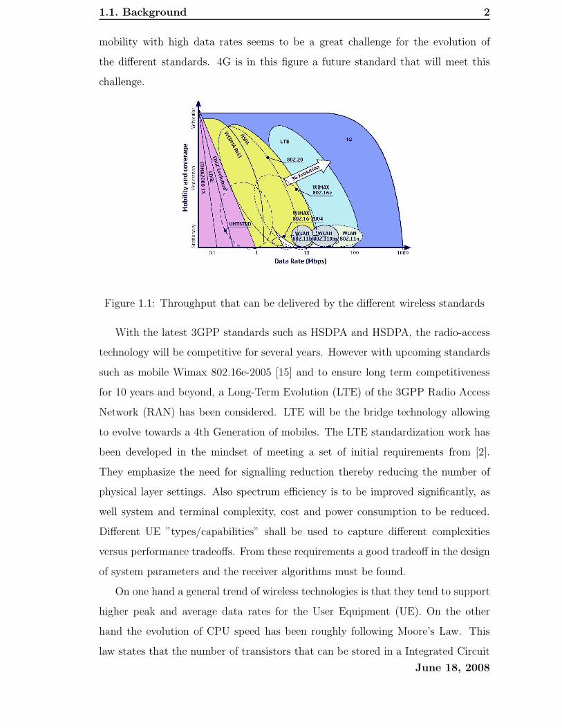
1.1 Throughput that can be delivered by the different wireless standards 2
2.1 Time-frequency representation of a transmitted OFDM signal [3] . . . 12
2.2 Principle of OFDM baseband signal generation . . . . . . . . . . . . . 13
2.3 Cyclic Prefix insertion . . . . . . . . . . . . . . . . . . . . . . . . . . 14
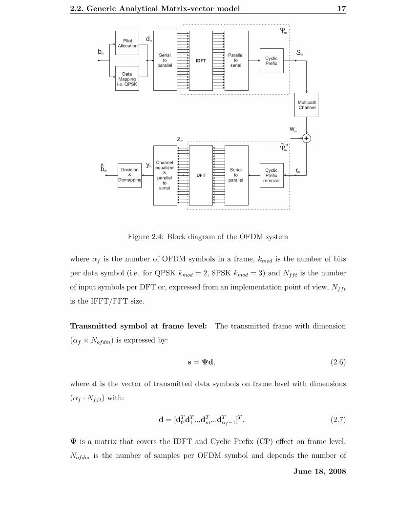
2.4 Block diagram of the OFDM system . . . . . . . . . . . . . . . . . . 17
2.5 Channel convolution with transmitted signal . . . . . . . . . . . . . . 21
3.1 Block diagram of the link level chain . . . . . . . . . . . . . . . . . . 30
3.2 LTE frame structure type 1 . . . . . . . . . . . . . . . . . . . . . . . 33
3.3 Maximum deliverable throughput in LTE for different physical layer
configurations . . . . . . . . . . . . . . . . . . . . . . . . . . . . . . . 36
3.4 without HARQ . . . . . . . . . . . . . . . . . . . . . . . . . . . . . 38
3.5 HARQ vs. no HARQ . . . . . . . . . . . . . . . . . . . . . . . . . 38
3.6 Maximal Spectral Efficiency for different MIMO schemes without
HARQ in a 10 MHz bandwidth . . . . . . . . . . . . . . . . . . . . . 38
4.1 Dual axis illustration of the weight function and an example PDP . . 42
4.2 SINR at receiver as a function of the CP length, Eb/No=15dB, Tu =
66, 67µs . . . . . . . . . . . . . . . . . . . . . . . . . . . . . . . . . . 44
4.3 SINR at receiver as a function of the CP length, Eb/No=30dB, Tu =
66, 67µs . . . . . . . . . . . . . . . . . . . . . . . . . . . . . . . . . . 45
4.4 Influence of the received SNR on CP length. Capacity for different
received signal powers, PDP= PedB Tu = 66, 67µs . . . . . . . . . . 46
xxi
List of Figures xxii
4.5 Influence of useful OFDM symbol length Tu on CP length Tg. Capac-
ity for different received signal powers, PDP= PedB, Eb/No=16dB . 47
4.6 Influence of the PDP on CP length Tg. Capacity for different channel
profiles, Eb/No=16dB . . . . . . . . . . . . . . . . . . . . . . . . . . 48
4.7 On the efficiency of the CP to cope with multipathTg . , Eb/No=16dB,
Tu = 66, 67µs, PDP= E4000 . . . . . . . . . . . . . . . . . . . . . . 49
5.1 Example of the time varying multipath described by a time varying
CIR and CTF . . . . . . . . . . . . . . . . . . . . . . . . . . . . . . . 54
5.2 Simplified block diagram of a baseband OFDM transmitter receiver
system . . . . . . . . . . . . . . . . . . . . . . . . . . . . . . . . . . . 58
5.3 2D FIR Wiener channel estimation for the mth CEB and nth subcarrier 60
5.4 Classical pilot grids . . . . . . . . . . . . . . . . . . . . . . . . . . . . 62
5.5 Diamond and diagonal pilot grids . . . . . . . . . . . . . . . . . . . . 62
6.1 Classification of Linear Frequency direction interpolation channel es-
timation algorithms in OFDM . . . . . . . . . . . . . . . . . . . . . . 67
6.2 Leakage of the NSS-CIR taps to the equivalent SS-CIR . . . . . . . . 76
6.3 Performance of the different estimators in a Full Bandwidth OFDM
system (Nu = Nfft = 2048) and a pilot spacing of 6 for the “long”
SS channel. (a) MSE. (b) BER. . . . . . . . . . . . . . . . . . . . . . 81
6.4 Performance of the different estimators in an LTE scenario with Nu =
1200, Nfft = 2048 and a pilot spacing of 6 for the “long” SS channel.
(a) MSE. (b) BER. . . . . . . . . . . . . . . . . . . . . . . . . . . . . 82
6.5 MSE of the ML estimator for varying assumed CIR length and dif-
ferent Nu, Nfft = 2048 and Eb/No = 15 dB . . . . . . . . . . . . . . 83
6.6 Effect of leakage on the classical algorithms in an LTE scenario with
Nu = 1200, Nfft = 2048 and a pilot spacing of 6 for the “long” NSS
channel. (a) MSE. (b) BER. . . . . . . . . . . . . . . . . . . . . . . 84
6.7 MSE of the ENRA with different delay estimation errors in an LTE
scenario with Nu = 1200, Nfft = 2048 and a pilot spacing of 6 for
the “long” NSS channel. . . . . . . . . . . . . . . . . . . . . . . . . . 85
June 18, 2008

List of Figures xxiii
6.8 Optimal Nm for MNRA in a nLTE scenario with Nu = 1200, Nfft =
2048 and a pilot spacing of 6 for the “long” and “short” NSS channels. 85
6.9 Performance of the MNRA with different α and optimal Nm in an
LTE scenario with Nu = 1200, Nfft = 2048 and a pilot spacing of 6
for the “long” and “short” NSS channels. (a) MSE. (b) BER. . . . . 87
6.10 TDLS . . . . . . . . . . . . . . . . . . . . . . . . . . . . . . . . . . . 91
6.11 ML and NRA . . . . . . . . . . . . . . . . . . . . . . . . . . . . . . . 91
6.12 ENRA and WF . . . . . . . . . . . . . . . . . . . . . . . . . . . . . . 91
6.13 RWF and SVD . . . . . . . . . . . . . . . . . . . . . . . . . . . . . . 91
7.1 Example of the stepwise 2 times 1D interpolation . . . . . . . . . . . 98
7.2 Proposed pilot schemes with different time domain spacings . . . . . 99
7.3 Full PedB . . . . . . . . . . . . . . . . . . . . . . . . . . . . . . . . . 102
7.4 Area of interest for PedB . . . . . . . . . . . . . . . . . . . . . . . . . 102
7.5 Full IndB . . . . . . . . . . . . . . . . . . . . . . . . . . . . . . . . . 102
7.6 Area of interest for IndB . . . . . . . . . . . . . . . . . . . . . . . . . 102
7.7 BER for different Frequency direction interpolation algorithms and
varying frequency direction pilot spacing (16QAM, Eb/No = 17dB,
10 MHz bandwidth). The right hand figures are higher resolution
simulations with a pilot spacing from 2 to 30 subcarriers. . . . . . . . 102
7.8 PER for varying G-Factor and velocity in a Typical Urban [46] profile
using P7, Wiener filtering and pilot frequency set to 8 . . . . . . . . . 104
7.9 Spectral Efficiency in DL LTE, Typical Urban [46], 10MHz . . . . . . 105
8.1 Spectral efficiency for different PDP with Tg = 4, 69µs, with a classi-
cal OFDM Linear Equalizer in a 10 MHz bandwidth . . . . . . . . . . 111
8.2 Interference cancelation schemes: (a) PIC, (b) SIC and (c) OSIC . . . 113
8.3 LE . . . . . . . . . . . . . . . . . . . . . . . . . . . . . . . . . . . . . 115
8.4 PIC . . . . . . . . . . . . . . . . . . . . . . . . . . . . . . . . . . . . 115
8.5 SIC . . . . . . . . . . . . . . . . . . . . . . . . . . . . . . . . . . . . . 115
8.6 OSIC . . . . . . . . . . . . . . . . . . . . . . . . . . . . . . . . . . . . 115
8.7 Uncoded BER vs. Eb/No with Ts = 7, 68ns, Nu = Nfft = 512, VehB 115
June 18, 2008
List of Figures xxiv
8.8 BER comparison of classical schemes for increasing iterations s . . . 116
8.9 2D contour plot of C0m . . . . . . . . . . . . . . . . . . . . . . . . . 117
8.10 2D contour plot of C1m . . . . . . . . . . . . . . . . . . . . . . . . . 117
8.11 3D mesh plot of C0m . . . . . . . . . . . . . . . . . . . . . . . . . . . 117
8.12 3D mesh plot of C1m . . . . . . . . . . . . . . . . . . . . . . . . . . . 117
8.13 Snapshot example of the log of the argument of the correlation matrices117
8.14 Matrix-vector illustration of two key steps in the LCIC algorithm: (a)
Initial one shot ISI removal, (b) Inner iteration k with ICI row removal 119
8.15 LCIC with different CP lengths for varying I and S = 2: (a) SNR=25dB,
(b) SNR=31dB . . . . . . . . . . . . . . . . . . . . . . . . . . . . . . 120
8.16 Complexity of the LCIC vs. the classical IC schemes for different I
values: (a)Evaluation for Nu=512 (b) LCIC gain for different NU . . 122
B.1 QPSK ECR 1/3 . . . . . . . . . . . . . . . . . . . . . . . . . . . . . . 143
B.2 16QAM ECR 1/2 . . . . . . . . . . . . . . . . . . . . . . . . . . . . . 144
B.3 64QAM ECR 5/6 . . . . . . . . . . . . . . . . . . . . . . . . . . . . . 144
C.1 IndoorA . . . . . . . . . . . . . . . . . . . . . . . . . . . . . . . . . . 147
C.2 Typical Urban . . . . . . . . . . . . . . . . . . . . . . . . . . . . . . . 147
C.3 Pedestrian B . . . . . . . . . . . . . . . . . . . . . . . . . . . . . . . . 147
C.4 Typical Urban, Quasi-fixed Nb of pilot subcarriers . . . . . . . . . . . 147
C.5 MSE in dB per subcarrier for the NRA algorithm in the case of an
Typical Urban profile for a fixed pilot spacing PS=6 . . . . . . . . . . 148
C.6 Estimated rank of (FHpsFps) . . . . . . . . . . . . . . . . . . . . . . . . 149
C.7 Zoom on the region of interest for Figure C.6 . . . . . . . . . . . . . . 149
C.8 Estimated rank of (FHpsFps), Nfft = 1024, PS=1 and varying Nu . . . 150
C.9 Maximum Ns for which the estimated rank of (FHpsFps) is equal to Ns 151
C.10 Average MSE for the NRA for a varying value of γ and different
number of used subcarriers . . . . . . . . . . . . . . . . . . . . . . . . 153
C.11 Singular Value analysis as a function of the CIR MED for a 5MHz
bandwidth using a linear scale . . . . . . . . . . . . . . . . . . . . . . 155
June 18, 2008

List of Figures xxv
C.12 Singular Value analysis as a function of the CIR MED for a 5MHz
bandwidth using a logaritmic scale . . . . . . . . . . . . . . . . . . . 155
D.1 BER for different Frequency direction interpolation algorithms and
varying frequency direction pilot spacing (16QAM, Eb/No = 17dB,
10 MHz bandwidth, Vehicular B). . . . . . . . . . . . . . . . . . . . . 157
D.2 Spectral efficiency for a 10 MHz bandwidth, Typical Urban PDP,
different ECR, Pilot scheme P1 at 3kmph, WF in frequency direction
and LI in time direction interpolation . . . . . . . . . . . . . . . . . . 158
D.3 Spectral efficiency for a 10 MHz bandwidth, Typical Urban PDP, dif-
ferent ECR, Pilot scheme P1 at 300kmph, WF in frequency direction
and LI in time direction interpolation . . . . . . . . . . . . . . . . . . 158
D.4 Spectral efficiency for a 10 MHz bandwidth, Typical Urban PDP, dif-
ferent ECR, Pilot scheme P2 at 300kmph, WF in frequency direction
and LI in time direction interpolation . . . . . . . . . . . . . . . . . . 159
D.5 Spectral efficiency for a 10 MHz bandwidth, Typical Urban PDP, dif-
ferent ECR, Pilot scheme P3 at 300kmph, WF in frequency direction
and LI in time direction interpolation . . . . . . . . . . . . . . . . . . 159
D.6 Spectral efficiency for a 10 MHz bandwidth, Typical Urban PDP, dif-
ferent ECR, Pilot scheme P4 at 300kmph, WF in frequency direction
and LI in time direction interpolation . . . . . . . . . . . . . . . . . . 160
D.7 Spectral efficiency for a 10 MHz bandwidth, Typical Urban PDP, dif-
ferent ECR, Pilot scheme P7 at 300kmph, WF in frequency direction
and LI in time direction interpolation . . . . . . . . . . . . . . . . . . 160
June 18, 2008
List of Tables
3.1 Different bandwidths and sampling frequencies in LTE . . . . . . . . 32
3.2 Perceived maximum Doppler frequencies at different speeds and car-
rier frequencies . . . . . . . . . . . . . . . . . . . . . . . . . . . . . . 34
3.3 FFT sizes for the different bandwidths . . . . . . . . . . . . . . . . . 35
3.4 Used set of MCS . . . . . . . . . . . . . . . . . . . . . . . . . . . . . 37
4.1 Exponential decaying channel PDP’s considered . . . . . . . . . . . . 43
6.1 Generalization of the algorithms . . . . . . . . . . . . . . . . . . . . . 73
6.2 Simulation parameters . . . . . . . . . . . . . . . . . . . . . . . . . . 79
6.3 Complexity for matrix and vector of dimensions (n · n) and (n). . . . 88
6.4 Complexity order of the different algorithms . . . . . . . . . . . . . . 89
7.1 Minimum frequency direction sample spacing for a 10MHz bandwidth 95
7.2 Minimum time direction sample spacing for a 10MHz bandwidth . . . 95
7.3 LTE parameters used for simulations . . . . . . . . . . . . . . . . . . 100
7.4 Performance loss due to ICI and estimation inaccuracy at 20 % PER 103
7.5 Total pilot overhead when ∆pf = 8 . . . . . . . . . . . . . . . . . . . 104
8.1 Complexity order for the studied IC schemes . . . . . . . . . . . . . . 121
A.1 ITU channel PDP’s considered . . . . . . . . . . . . . . . . . . . . . . 139
A.2 Hilly Terrain channel PDP . . . . . . . . . . . . . . . . . . . . . . . . 140
A.3 Channel Power Delay Profiles . . . . . . . . . . . . . . . . . . . . . . 141
B.1 Main link simulation assumption . . . . . . . . . . . . . . . . . . . . 143
xxvi
Chapter 1
Introduction
1.1 Background
Many different wireless technologies exist on the market or are planned to be rolled
out within the next years. One can distinguish roughly between ”mobile” and
”static/nomadic” wireless technologies, where the main difference is that the latter
doesn’t support handover between access points. The second generation (2G) and
third generation (3G) of mobile phones support ”mobility”, whereas the ”nomadic”
technologies are more oriented towards providing broadband packet-data access,
such as fixed Wimax 802.16-2004 [14]. Yet the ”nomadic” technologies are outside
the scope of this work. The ”mobile” 2G technologies such as GSM, GPRS and
EDGE are giving theoretical downlink peak data rates of respectively 9,6 kbit/s, 80
kbit/s and 236,8 kbit/s, whereas the ”mobile” 3G technologies such as WCDMA
and HSDPA are giving theoretical downlink peak data rates of respectively 384
kbit/s and 14,4 Mbit/s. These will potentially go up to 42 Mbit/s with the second
phase of HSDPA (HSPA Evolved) being specified in the upcoming 3GPP release 7.
In a longer time frame perspective a fourth generation (4G) of mobile phones will
arise. This 4G is officially not defined, but is estimated to become a high data rate
technology supporting inter-Radio Access Technology (inter-RAT) handover with
more than 100 Mbit/s for outdoor and 1 Gbit/s for indoor downlink data rates. In
Figure 1.1 an overview over the different wireless technologies, existing and planned,
is given. The different 2G and 3G wireless technologies can be situated. Combining
1
1.1. Background 2
mobility with high data rates seems to be a great challenge for the evolution of
the different standards. 4G is in this figure a future standard that will meet this
challenge.
Figure 1.1: Throughput that can be delivered by the different wireless standards
With the latest 3GPP standards such as HSDPA and HSDPA, the radio-access
technology will be competitive for several years. However with upcoming standards
such as mobile Wimax 802.16e-2005 [15] and to ensure long term competitiveness
for 10 years and beyond, a Long-Term Evolution (LTE) of the 3GPP Radio Access
Network (RAN) has been considered. LTE will be the bridge technology allowing
to evolve towards a 4th Generation of mobiles. The LTE standardization work has
been developed in the mindset of meeting a set of initial requirements from [2].
They emphasize the need for signalling reduction thereby reducing the number of
physical layer settings. Also spectrum efficiency is to be improved significantly, as
well system and terminal complexity, cost and power consumption to be reduced.
Different UE ”types/capabilities” shall be used to capture different complexities
versus performance tradeoffs. From these requirements a good tradeoff in the design
of system parameters and the receiver algorithms must be found.
On one hand a general trend of wireless technologies is that they tend to support
higher peak and average data rates for the User Equipment (UE). On the other
hand the evolution of CPU speed has been roughly following Moore’s Law. This
law states that the number of transistors that can be stored in a Integrated Circuit
June 18, 2008

1.2. Purpose of LTE 3
for minimum component cost doubles every 24 months [17]. However the size of a
single transistor can’t be reduced indefinitely, and will be limited by the atomic size
of approximately 0,1 nm. Moore’s Law is therefore bound to break and CPU speed
evolution will slow down. As the need for higher transmission data rates doesn’t
seem to slow down, and with the growth of CPU speed slowing down, the need for
efficient baseband signal processing algorithms will strongly increase.
After considering the trends of the LTE requirements and the evolution of
Moore’s law, a key aspect of this thesis will be how to design new system param-
eters and receiver algorithms in a way that requirements are fulfilled and receivers
feasible.
1.2 Purpose of LTE
3GPP LTE is the name of a project within the 3GPP which aim is to enhance the
UMTS standard and to deal with future requirements. These future requirements
will need improvements of several key areas such as: efficiency, operator costs, better
and new services, usage of available spectrums and better integration with other
standards and will result in release 8 of the 3GPP standards. When presenting LTE
a broad question arises: ”What is the purpose of LTE?”.
In this section we will attempt to answer to this question without too many
technical details. The purpose of LTE is to develop a set of specifications that will
be the basis of a framework for the evolution of the 3GPP radio-access technology.
These should allow a high data rate, low latency and packet optimized radio access
technology. In the following, the different goals of LTE relevant to this Ph.D. thesis
will be listed:
• Flexible/scalable transmission bandwidth. It will go from 1,25 MHz
up to 20 MHz in order to allow a flexible technology cohabitation with other
standards. This will imply that the different algorithms should be flexible,
adaptive and optimized for the different proposed bandwidths.
• High peak data rates: 100 Mbps in downlink. In this case it will require
low complexity algorithms as the available computational complexity at the
June 18, 2008

1.3. Goals and Limitations 4
UE per received bit will be low.
• Increased cell edge bitrate maintaining site locations as in WCDMA.
This will be a vital consideration for the operator. There is no interest in
increasing the amount of expensive base stations to cover a given area.
• Improved spectrum efficiency. The improvement should be of 2 to 4 times
the one of Release 6 HSPA. Higher order modulation schemes (16QAM and
64QAM) as well as spatial multiplexing MIMO are required to achieve these
requirements.
• Reduced Radio-access network latency. Possibility of latency below 10
ms. When looking at the physical layer, this goal has influence on the avail-
able estimation and data detection time, setting some tight requirements for
algorithm implementation.
• Reasonable system and terminal complexity, cost and power con-
sumption. This will result in many tradeoff decisions when looking at the
parameter design and algorithmic choices to be made.
• System optimized for low mobile speed but should also support high
mobile speeds. For a slowly fading radio channel the performance should be
maximized without penalizing the functionality at high speeds.
1.3 Goals and Limitations
1.3.1 Goals
The goals of this Ph.D. thesis are set within the context of a ”generic OFDM base-
band model” with application to a ” specific LTE scenario”. In this way the analyti-
cal results can be extended to other OFDM based systems, and the practical results
will show the applicability of the generic models and solutions to LTE. The goals of
this thesis are several. First the impact of key physical layer parameters on system
performance should be studied namely the CP length and the pilot scheme design.
June 18, 2008

1.3. Goals and Limitations 5
Secondly the impact of these key parameter on receiver algorithm design should be
investigated in several channel scenarios.
In order to achieve these goals several steps need to be carried out, among which
are careful system modeling, simulator development, realistic simulations as well as
algorithm investigation. To achieve the desired goals, each of the above steps are
guided by key questions in the following.
First, within an analytical context, we would like to know ”what is a good choice
of OFDM baseband matrix-vector model?” More specifically the mathematical as-
sumptions behind the modeling should be elaborated. From these assumptions a
generic discrete model should be derived describing the baseband signal from the
point of transmission until reception, including the effects of the multipath channel
and gaussian noise.
When these models are established, the simulation context should be elaborated
starting with understanding ”how have the key OFDM physical layer parameters
have been chosen in LTE?”. A simulator environment supporting the 3GPP LTE
parameters should be developed. This will enable us to answer to ” what will the
baseline LTE performance be in terms of Spectral Efficiency?”
The analytical modeling as well a performance of an OFDM system strongly
depends on the physical channels models considered, as well as the length of the
Cyclic Prefix. Therefore before undergoing an in depth algorithmic study in this
thesis, we will try to answer ”how shall the Cyclic Prefix length be chosen?”. This
will present an interesting tradeoff between transmission overhead and multi-path
robustness.
Once the modeling and the simulation scene is established, the in depth algorith-
mic study can follow. When dealing with PACE and the classical signal model, we
would like to know ”how performance is affected by different OFDM channel estima-
tion algorithms? What will be the most efficient tradeoffs between these algorithms
in a LTE-OFDM context?”. The scope of this study will be focused on linear al-
gorithms. The introduction of virtual subcarriers as well as the leakage effect, due
to non-sample-spaced PDP, is considered in an algorithm comparison. From perfor-
mance results as well as a complexity study, solutions for practical implementation
June 18, 2008
1.3. Goals and Limitations 6
will be suggested for LTE.
A choice of channel estimation algorithms will then set the baseline to determine
”how the pilot scheme and spacing shall be chosen for LTE?” Time and frequency di-
rection pilot spacing will be considered. Theoretical results derived from the Nyquist
sampling theorem will be compared to practical performance results.
Considering the advanced novel signal model, we will then study ”what is the
effect of a longer impulse response than the CP length on Spectral Efficiency and
how well can interference cancelation compensate for a short CP length?”. When the
CIR is longer than the CP the classical OFDM signal model is no longer accurate
and the one tap equalizer is insufficient. Usage of classical Multiuser Detection
(MUD) algorithms such as the Zero Forcer (ZF) or Minimum Mean Square Error
(MMSE) approaches are computationally prohibitive. Therefore the special case of
OFDM with Inter Carrier Interference (ICI) and Inter Symbol Interference (ISI),
will be studied carefully and the equalization process will be enhanced with specific
interference cancelation schemes.
1.3.2 Limitations
To narrow down the scope of the thesis and in order to focus in depth on the given
topics, a few limitations have been established for the given work. They are given
by:
• Performance evaluation will mainly be carried out using the downlink LTE
settings given by the frame structure type 1 in FDD mode defined in 3GPP
TS 36.211 [3].
• The focus of this thesis limits the study to FDD where all subframes are
available for downlink transmission.
• Specific channel power delay profiles defined in the appendix A will be used
for monte-carlo simulations.
• Single Input Single Output (SISO) antenna constellation is considered in all
chapters.
June 18, 2008
1.4. Methodology 7
• The modeling assumes perfect synchronization or the received signal in time
and frequency domains.
• The PACE algorithms studied assume a Cyclic Prefix (CP) length longer than
the maximum excess delay of the PDP and and a constant channel during the
duration of 1 OFDM symbol
• The performance results are all single user results assuming one user having full
usage of all downlink bandwidth available. Thereby no OFDMA or resource
sharing is considered.
1.4 Methodology
During this thesis a pragmatic methodology has been adopted in order to achieve
the goals. The strategy behind attacking the different posed problems has been
based on an iterative approach. The methodology adopted can be summarized in
the following order:
1. A state of the art is established from an extensive survey in the field of inves-
tigation.
2. The assumptions and limitations of the problems are clearly stated.
3. A mathematical matrix-vector model of the received OFDM signal is derived
with the desired level of modeling detail.
4. A performance study of state of the art solutions is conducted within the area
chosen.
5. A solution or new improved scheme is proposed.
6. A performance comparison of the proposed solution is carried out with the
state of the art reference(s).
This process can then be iterated increasing the level of detail of the OFDM received
signal model or changing the initial assumptions. Thereby the experience acquired
during the first iteration can be used to refine the second iteration.
June 18, 2008
1.5. Outline and Organization of the Thesis 8
1.5 Outline and Organization of the Thesis
This thesis consists of 9 chapters and 3 appendices. The two main topics dealt
with are parameter design and algorithm investigation. As these two topics depend
on each other, and, at the same time are strongly influenced by the LTE system
requirements, they are dealt with in an alternate order.
Chapter 1 gives an introduction to the thesis consisting of several sub-topics.
A general technical background of the content, relevant LTE 3GPP specifications,
goals and limitations will help in defining the thesis with a given scope and aim. A
stress on the methodology used is followed by an outline, a list of publications and
a list of inventions filed during this thesis.
Chapter 2 mainly covers OFDM basics, as well as an in depth modeling of the
signal from transmitter to receiver side. The modeling work ends up with two
relevant signal models: A classical, well known interference-free model, and a novel
generic advanced model taking ISI an ICI into consideration.
Chapter 3 describes the two simulators developed during this work. The first
simulator focuses on delivering quick simulations results as it doesn’t have any outer
receiver features such as error control coding. This first simulator will give MSE,
uncoded BER and SINR results. The author has developed the core of this simula-
tor, namely the Tx/Rx modules, the channel models and convolution. Much effort
has also been spent on receiver algorithms and parameter design together with the
authors former Master students Guillaume Monghal and Carles Navarro Manchon as
illustrated in their respective master thesis [51] and [52]. A second link level UTRA-
LTE simulator has been developed jointly with other Ph.D. students: W. Na, A.
Pokhariyal and B.E. Prianto. Basic performance in terms of spectral efficiency of
different modulation schemes is carried out in a 10MHz scenario. Validation of both
simulators is given in appendix B.
Chapter 4 is an independent CP length study aimed at an LTE configuration.
The dual nature of the CP (cancels interference but introduces system overhead) is
discussed and the optimal CP length is elaborated for different channel and param-
eter conditions.
Chapter 5 presents the Pilot Assisted Channel Estimation (PACE) problematic
June 18, 2008
1.6. Publications and Invention disclosures 9
for OFDM. The nature and statistics of the radio channel are discussed and a channel
estimation strategy proposed for LTE. This strategy will guide the structure and
content of chapter 6 and of chapter 7.
Chapter 6 is the most extensive of this thesis and focuses on frequency direc-
tion PACE for OFDM. An extensive state-of-art is made from previous research.
The lacks of previous comparisons are stressed and a generic unified formulation is
developed to conduct a novel fair comparison of algorithms. Results show a clear
relationship between a-priori information considered at the Rx side, and the per-
formance obtained. Two algorithms are recommended for LTE: the robust wiener
filter [78] and the true parametric wiener filter [75].
Chapter 7 investigates different pilot patterns and pilot densities for LTE. From
the PACE strategy defined in chapter 5 a pilot spacing design method is proposed
to determine which efficient scheme to be used in LTE.
Chapter 8 proposes to shorten the CP length used in OFDM by means of op-
timized interference cancelation techniques. A iterative, reduced complexity algo-
rithm with fast convergence rate and tractable complexity is developed: the LCIC
algorithm.
Chapter 9 concludes the thesis work and elaborates on possible future research
topics.
1.6 Publications and Invention disclosures
The following articles have been published during the Ph.D. study:
• C. Rom, T.B. Sørensen, P.E. Mogensen and B. Vejlgaard, ”Impact of Cyclic
Prefix length on OFDM system Capacity”, Proceedings of the WPMC’05 Vol.3,
pp. 1871-1875, 18-22 September 2005
• C. Rom, C. N. Manchon, T.B. Sørensen, P.E. Mogensen and Luc Deneire,
”Analysis of Time and Frequency Domain PACE Algorithms for OFDM with
Virtual Subcarriers” Personal, Indoor and Mobile Radio Communications,
2007 IEEE 18th International Symposium Sept. 2007 Pages: 1-5
June 18, 2008
1.6. Publications and Invention disclosures 10
• C. Rom, C. N. Manchon, T.B. Sørensen, P.E. Mogensen and Luc Deneire,
”Unification of Frequency direction Pilot-symbol Aided Channel Estimation
(PACE) for OFDM,” 10th International Symposium on Wireless Personal
Multimedia Communications Vol.XX, pp. xxxx-xxxx, 03-06 September 2007
• G. Monghal, Y. Malidor, C. Rom and T.B. Sørensen, ”Low Complexity Inter-
ference Cancellation applicable to OFDM with a Short Cyclic Prefix”, Pro-
ceedings of the WPMC’05 Vol.2, pp. 1032-1035, 18-22 September 2005
• A. Veiverys, V.P. Goluguri, Y. Le Moullec, C. Rom, O. Olsen, P. Koch,
”A Generic Hardware-Accelerated OFDM System Simulator”, IEEE Norchip
2005, 21-22 November 2005, Oulu, Finland
• B.E. Priyanto, C. Rom, C.N. Manchon, T.B. Sørensen, P.E. Mogensen, ”Ef-
fect of Phase Noise on Spectral Efficiency for UTRA Long Term Evolution”
Personal, Indoor and Mobile Radio Communications, 2006 IEEE 17th Inter-
national Symposium Sept. 2006 Pages:1 - 5
• N. Wei, A. Pokhariyal, C. Rom, B.E. Priyanto, F. Frederiksen, C. Rosa, T.B.
Sørensen, T. Kolding and P.E. Mogensen, ”Baseline E-UTRA Downlink Spec-
tral Efficiency Evaluation” Proceedings of 2006 IEEE 64th Vehicular Technol-
ogy Conference 2006
The following inventions have been submitted to Infineon Technologies during the
Ph.D. study:
• Low Complexity Interference Cancellation scheme for Orthogonal Frequency
Division Multiplexing receivers, April 2005
• Aufwandsgnstige Kanalschatzung mit hoher Gute fur Merhtragerfunksysteme
(OFDM), April 2006
• Wireless communications system using pre-equalisation based on terminal lo-
cation estimates, June 2006
• Threshold-Based Channel Tracking for Enhanced Noise Reduction in OFDM,
July 2006, accepted for Patent
June 18, 2008
Chapter 2
OFDM modelling
OFDM (Orthogonal Frequency Division Multiplexing) has shown many interesting
properties for wireless data transmission such as spectral efficiency, low complex
transceivers and robustness over time dispersive channels. Also, OFDM has been
chosen to be the downlink multiple access scheme in LTE. The purpose of this
chapter is to give some general information regarding OFDM basics, including its
definition, signal generation, CP insertion, parameter relationships, reception and
signal properties and the advantages and disadvantages of this modulation scheme.
A generic discrete matrix-vector analytical model of the received signal will be de-
rived, which can be simplified into the classical model used for PACE OFDM.
2.1 OFDM basics
OFDM is a technology that has been shown to be well suited to the mobile radio
environment for high rate and multimedia services. A worldwide convergence has
occurred and OFDM has appeared as an emerging technology in many standards.
Examples of commercial OFDM systems include WLANs such as the 802.11a/g [8]
[9] [10] amendment to Wi-Fi, Digital Audio Broadcast (DAB) systems [11], Digital
Video Broadcast TV systems such as DVB-T [12], DVB-H [13], T-DMB and ISDB-
T, the IEEE 802.16 WiMAX Wireless MAN [14] [15], the IEEE 802.20 or Mobile
Broadband Wireless Access (MBWA) system and the Flash-OFDM system. Much
research has been done in the field of OFDM based physical layer [18] [19] [20], and
11

2.1. OFDM basics 12
it can be classified as a mature research topic.
Figure 2.1: Time-frequency representation of a transmitted OFDM signal [3]
Definition: This technique is based on the well-known technique of Frequency
Division Multiplexing (FDM). The OFDM technique transmits data over multiple
carriers (from now on called subcarriers) that contain the information stream. These
sub-carriers are orthogonal to each other in both time and frequency domains. How-
ever to compensate for radio channel multipath transmission delays, a guard time,
called Cyclic Prefix (CP) is usually added to each OFDM symbol to combat the
resulting interference as suggested in [3]. This technique, illustrated in figure 2.1,
transforms a frequency-selective wide-band channel into a group of non-selective
narrowband channels, which make CP-OFDM robust against large delays of the
signal due to multipath.
Signal Generation: In this study information bits are linearly modulated into
data symbols using for example Quadrature Phase Shift Keying (QPSK) or Quadra-
ture Amplitude Modulation (QAM). The modulated symbols are then transmit-
ted over closely spaced orthogonal subcarriers. The orthogonality is generated
through the use of orthogonality functions, equally spaced in frequency, that are
synchronously applied to the modulated data symbols. The transmitted baseband
signal, as illustrated in figure 2.2, is then given by:
sm(t) =Nu−1∑
k=0
dm,kψk(t), (2.1)
June 18, 2008

2.1. OFDM basics 13
where, ψk(t) = 1√Tuej2πfkt is the basic orthogonality function applied to the kth
subcarrier. In classical literature these functions are also named tones at frequency
fk. Nu and Tu are respectively the number of used subcarriers and the OFDM
symbol duration and dm,k the transmitted data symbol for the kth subcarrier and
mth OFDM symbol.
QAM/QPSK
modulator
QAM/QPSK
modulator
QAM/QPSK
modulator
.
.
.
.
?
Y(t)k
Y(t)0
Y(t)N 1u-
s(t)
IFFT
Figure 2.2: Principle of OFDM baseband signal generation
An advantage of OFDM is that the modulation of the orthogonality functions
can be performed using an IFFT thereby significantly reducing the computational
complexity required for a large transmission bandwidth.
Cyclic Prefix insertion When transmitted over a multi-path channel, the OFDM
signal is subject to Inter Symbol Interference (ISI) and Inter Carrier Interference
(ICI) caused by the time-dispersive channel. A guard interval is therefore inserted
prior to the useful OFDM symbol as seen in figure 2.3. In order to maintain orthogo-
nality between subcarriers and their delayed replicas, the last Ng samples are copied
at the beginning of each OFDM symbol. The orthogonality function is extended
and becomes:
ψk(t) =
1√Tuej2πfk(t+Tu) −Tg ≤ t < 0,
1√Tuej2πfkt 0 ≤ t < Tu,
0 otherwise
At the receiver a matched filter is applied to retrieve the useful signal energy.
June 18, 2008

2.1. OFDM basics 14
TuTg
Tofdm
duplication
Figure 2.3: Cyclic Prefix insertion
This is done by integration with the complex conjugated orthogonality function:
∫ Tu
0
ψk(t)ψ∗k′(t)dt =
1 k = k′,
0 k 6= k′.
If delayed versions of the signal are received then for the replica delayed by τ :
∫ Tu
0
ψk(t− τ)ψ∗k′(t)dt =
1 k = k′, τ ≤ Tg
ρ k = k′, τ > Tg
0 k 6= k′, τ ≤ Tg
ρ′ k 6= k′, τ > Tg.
This means that the kth orthogonality function is robust against correlation with
any k′th other orthogonality function as long as the maximum excess delay of the
channel Tmed is smaller than the CP duration Tg. When the delays are larger than
Tg, the orthogonality is destroyed and a non zero output results.
Parameter relationships When looking at OFDM without the insertion of a
guard period, a classical design tradeoff lies in the relationship between subcarrier
width ∆k and OFDM symbol time Tu (in this case Tg = 0, Tu = Tofdm), which is
given by:
∆k =1
Tu
. (2.2)
Two main channel distortion sources are the multipath delay spread, usually statis-
tically characterized by the RMS delay spread τrms and the Doppler spread charac-
terized by the coherence time tcor (related to the Doppler frequency fd = 1tcor
). In
June 18, 2008
2.1. OFDM basics 15
order to have robustness against excess delays, one would need:
Tu ≫ τrms. (2.3)
On the other hand in order to limit ICI due to fast fading:
Tu ≪ tcor. (2.4)
The classical OFDM approach to determine Tu and ∆k is a tradeoff between the
UE speeds and the delay spreads supported. However when a CP is inserted and
Tg > Tmed, then the loss of orthogonality of subcarriers due to multipath spread is
completely canceled. This leaves a large freedom of design of parameters in CP-
OFDM, where mostly the subcarrier spacing versus supported Doppler frequencies
needs to be considered. Note that the subcarrier spacing will indirectly affect the
SEL loss due to CP overhead an can therefore not be indefinitely large.
Pros and cons of OFDM In the following, the main advantages and disadvan-
tages of OFDM will be stated. Among the advantages of OFDM the next can be
highlighted:
• Low complex equalizer at signal reception. When the CP length is longer
than the maximum excess delay, and the effect due to Doppler distortion is
negligible, the optimal equalization in SISO, only needs one complex operation
per subcarrier [18] [19].
• Easy combination with MIMO enabling high spectral efficiencies.
• Adapts easily to varying mobile wireless channels through convenient choice
of CP length, number of subcarriers and FFT length.
• Flexible bandwidth scalability allowing an easier cohabitation with other pre-
viously installed communication systems.
• Robust against narrowband interference as only a few subcarriers will be af-
fected.
Among the disadvantages of OFDM can be highlighted:
June 18, 2008
2.2. Generic Analytical Matrix-vector model 16
• Peak-to-Average Power Ratio (PAPR) problematic.
• Sensitivity to synchronization.
• Reduced spectral efficiency due to CP.
2.2 Generic Analytical Matrix-vector model
This subsection will give a discrete-time description of the OFDM signal from trans-
mission to reception at baseband level. In a first step a ”novel generic model” is
developed. It is generic in the sense that the assumptions are broad and few limita-
tions are made. The signal is considered time variant at a resolution of the receiver
sampling time Ts and the maximum excess delay of the CIR is shorter than the
useful OFDM symbol time Tu. The model is also generic in the sense that different
levels of modeling are targeted: frame level, OFDM symbol level and sample level.
Generic model:
A block diagram of the downlink baseband OFDM system is given in Fig.2.4. The
bold vectors are expressed in matrix-vector notation in three levels:
• Frame level being the starting point and showing the relationship between the
data transmitted through the physical channel and the data decoded at the
receiver.
• OFDM symbol level showing the details of a symbol by symbol transmission.
• Sample level will be the lowest level providing an accurate tool for investigation
and implementation enhancements.
The developed mathematical model will then follow the data flow of the trans-
mission block diagram. The data bits to be transmitted are sent in blocks, and
expressed by a vector:
b = (b[0],b[1]...b[n]...b[αfkmod(Nfft − 1)]), (2.5)
June 18, 2008
2.2. Generic Analytical Matrix-vector model 17
bm
DataMappingi.e. QPSK
PilotAllocation
dm
Serialto
parallelIDFT
Parallel
erialto
s
CyclicPrefix
Sm
Ym
MultipathChannel
wm
rmSerial
toparallel
DFT
Channelequalizer
¶llel
toserial
CyclicPrefix
removal
Ym
~ H
zm
ym
Decision&
Demapping
bm^
Figure 2.4: Block diagram of the OFDM system
where αf is the number of OFDM symbols in a frame, kmod is the number of bits
per data symbol (i.e. for QPSK kmod = 2, 8PSK kmod = 3) and Nfft is the number
of input symbols per DFT or, expressed from an implementation point of view, Nfft
is the IFFT/FFT size.
Transmitted symbol at frame level: The transmitted frame with dimension
(αf ×Nofdm) is expressed by:
s = Ψd, (2.6)
where d is the vector of transmitted data symbols on frame level with dimensions
(αf ·Nfft) with:
d = [dT0 dT
1 ...dTm...d
Tαf−1]
T . (2.7)
Ψ is a matrix that covers the IDFT and Cyclic Prefix (CP) effect on frame level.
Nofdm is the number of samples per OFDM symbol and depends the number of
June 18, 2008
2.2. Generic Analytical Matrix-vector model 18
CP samples Ng and the number of used subcarrier samples Nu. The dimensions of
Ψ are (αf · Nofdm) × (αf · Nfft) and will be further explained in the symbol level
subsection. We have:
Ψ =
Ψ0 0 . . . 0
0. . .
... Ψm
.... . . 0
0 . . . 0 Ψαf−1
. (2.8)
Transmitted OFDM symbol at symbol level: The mth transmitted OFDM
symbol is expressed as follows:
sm = Ψmdm (2.9)
where Ψm is a sub-matrix of dimension (Nofdm × Nfft). It performs an IDFT of
the input symbol sequence dm and adds a redundant CP of size Ng. We have the
relation: Nofdm = Nfft +Ng.
Ψm = (ΨTm,0Ψ
Tm,1...Ψ
Tm,k...Ψ
Tm,Nfft−1) (2.10)
ΨTm,k is the kth orthogonality vector.
Having the relationship fk = k Fs
Nfft, a convenient expression with CP is given by:
Ψm,k[n] =1
√
Nfft
ej2πk(
n−Ng
Nfft), (2.11)
with, Ψm,k = (Ψm,k[0],Ψm,k[1], ...Ψm,k[Nofdm−1]), and dm = (dm[0],dm[1], ...dm[Nfft−
1]) is a vector containing Nfft data symbols to be transmitted in the mth OFDM
symbol, where fk is the kth sub-carrier frequency, Fs is the sampling frequency. Some
of the elements of dm could be set to zero, thereby allowing the model to include
virtual subcarriers.
Without CP we have:
sm = Ψmdm ⇐⇒ sm = IDFT{dm} (2.12)
since
Ψm,k[n] =1
√
Nfft
ej2πfkn
Fs . (2.13)
June 18, 2008

2.2. Generic Analytical Matrix-vector model 19
Transmitted OFDM symbol at sample level: Each baseband transmitted
sample can be expressed as:
sm[n] =
Nfft−1∑
k=0
Ψm,k[n]dm[k], (2.14)
where each subcarrier is multiplied with the corresponding data symbol, and then
the product is summed for each subcarrier sample.
Received signal at frame level: The received signal vector r, of dimension
(αf ×Nofdm) during the transmission of a full frame, can be expressed as:
r = Hs + w, (2.15)
where, H is the channel convolution matrix of dimensions (αf ·Nofdm)× (αf ·Nofdm)
expressed as:
H =
H00 0 . . . 0
H10 H01 0
0 H11. . .
...
0. . .
... H0αf−2 0
0 H1αf−2 H0αf−1
. (2.16)
H0m and H1m are matrices of dimension (Nofdm × Nofdm) and will be defined in
the following, s is the transmitted frame of dimension (αf × Nofdm) and w is the
Additive White Gaussian Noise (AWGN) vector of same dimension (αf × Nofdm),
with µw = E{w} = 0 and Rww = E{wwH} = σ2wI.
Received signal at OFDM symbol level: The received signal vector rm, of
dimension (Nofdm), at symbol level can be expressed as:
rm = H1m−1sm−1 + H0msm + wm. (2.17)
June 18, 2008

2.2. Generic Analytical Matrix-vector model 20
Given that the maximum length of the impulse response is limited to Nofdm samples,
the sub-matrices H0m and H1m are defined as:
H0m =
lm,0[0] 0 . . . 0
lm,1[0] lm,0[1]
lm,1[1] 0...
.... . .
... lm,0[Nofdm − 2] 0
lm,Nofdm−1[0] lm,Nofdm−2[1] . . . lm,1[Nofdm − 2] lm,0[Nofdm − 1]
.(2.18)
H1m =
0 lm,Nofdm−1[1] lm,Nofdm−2[2] . . . lm,1[Nofdm − 1]
0 0 lm,Nofdm−2[2] lm,2[Nofdm − 1]
0...
.... . .
lm,Nofdm−1[Nofdm − 1]
0 . . . 0
. (2.19)
lm,p[n] is the pth discrete sample-spaced complex tap coefficient at sample instant
n of the mth OFDM symbol.
Received signal at OFDM sample level: One way of representing the multi-
path effect is done through a time representation of the arrival of the transmitted
symbols for all the resolvable paths. A visualization of this channel convolution is
shown in Fig.2.5. One can observe the same signal arriving at different delays, some
within the timing of the CP others arriving later than the duration of the CP.
At sample level the received signal can be expressed as:
rm[n] =
n∑
p=0
lm,p[n− p]sm[n− p]
+
Nofdm−1∑
i=n+1
lm−1,i[Nofdm + n− i]sm−1[Nofdm + n− i] (2.20)
It is noted that equation 2.20 assumes that the delays are smaller than an OFDM
symbol length.
June 18, 2008
2.2. Generic Analytical Matrix-vector model 21
Tofdm
N -1ofdm
N -1g
Ng
N +1g
0
TgT=0
Sm+1SmSm-1
rm+1rm-1 rm
zm zm+1zm-1
YmYm Ym~ H~ H~ H
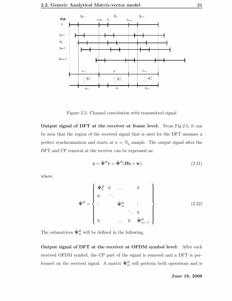
Figure 2.5: Channel convolution with transmitted signal
Output signal of DFT at the receiver at frame level: From Fig.2.5, it can
be seen that the region of the received signal that is used for the DFT assumes a
perfect synchronization and starts at n = Ng sample. The output signal after the
DFT and CP removal at the receiver can be expressed as:
z = ΨHr = ΨH(Hs + w), (2.21)
where,
ΨH =
ΨH0 0 . . . 0
0. . .
... ΨHm
.... . . 0
0 . . . 0 ΨHαf−1
. (2.22)
The submatrices ΨHm will be defined in the following.
Output signal of DFT at the receiver at OFDM symbol level: After each
received OFDM symbol, the CP part of the signal is removed and a DFT is per-
formed on the received signal. A matrix ΨHm will perform both operations and is
June 18, 2008

2.2. Generic Analytical Matrix-vector model 22
defined as:
ΨHm,k[n] =
ΨHm,n[k] if n > Ng,
0 else.
The output of the DFT can then be expressed as:
zm = ΨHmrm = ΨH
m(H1m−1sm−1 + H0msm + wm), (2.23)
where, ΨHm is equal to ΨH
m with the CP elements set equal to zero. Multiplying
the data to be transmitted by ΨHm is equal to perform an IDFT and to add a CP.
Multiplying the received signal with ΨHm is equal to remove the CP and perform a
DFT.
It is then possible to describe the received OFDM signal at symbol level in a
more intuitive way. The impact of the time and frequency selective physical channel
is given by one single equation:
zm = C1m−1dm−1 + C0mdm + ΨHmwm (2.24)
with,
C1m−1 = ΨHmH1m−1Ψm−1
C0m = ΨHmH0mΨm
The effects of the ISI (zISI,m) and the ICI (zICI,m) can then be separated from the
desired signal (zS,m) by:
zm = zISI,m + zICI,m + zS,m + ΨHmwm. (2.25)
We have:
zISI,m = C1m−1dm−1,
zICI,m = C0ICI,mdm,
zS,m = C0S,mdm,
(2.26)
where,
C0ICI,m[k′, k] =
C0m[k′, k] if k′ 6= k,
0 if k′ = k,
and
C0S,m[k′, k] =
0 if k′ 6= k,
C0m[k′, k] if k′ = k.
June 18, 2008

2.3. Classical Analytical Matrix-vector model 23
Output signal of DFT at the receiver at sample level: At sample level the
signal after the DFT can be expressed as follows:
zm[k′] =
Nofdm−1∑
k=0
C1m−1[k′, k]dm−1[k] + C0m[k′, k]dm[k] + ΨH
m,k′ [k]wm[k], (2.27)
with each element of the correlation matrices given as:
C0m[k′, k] =
Nofdm−1∑
n=0
Ψ∗m,k′[n]
n∑
i=0
lm,i[n− i]Ψm,k[n− i], (2.28)
and
C1m[k′, k] =∑Nofdm−2
n=0 Ψ∗m,k′[n]
·∑Nofdm−1
i=n+1 lm−1,i[Nofdm + n− i]Ψm−1,k[Nofdm + n− i].(2.29)
2.3 Classical Analytical Matrix-vector model
The previous general model can be brought into a more commonly used model by
assuming that the CIR is stationary during the transmission time of an OFDM
symbol and that the maximum excess delay is shorter than the CP length. These
assumptions allow a major simplification leading to the standard OFDM model
encountered for most OFDM-based publications such as [26] [27] and [28].
The received signal after the DFT can be simplified to:
zm = C0S,mdm + wm. (2.30)
By introducing the Channel Transfer Function (CTF) vector hm = Fgm, where F
is a DFT matrix of dimension (Nfft ·Nfft) and gm is the CIR vector of dimension
(Nfft · 1), we have the relationship:
C0S,m[k, k] = hm[k]. (2.31)
The received signal after DFT can the be rewritten as:
zm = Dmhm + wm, (2.32)
and at sample level gives:
zm[k] = Dm[k, k]hm[k] + wm[k]. (2.33)
June 18, 2008
2.3. Classical Analytical Matrix-vector model 24
The discrete signal after the one tap equalizer at sample level is then:
ym[k] =zm[k]
hm[k], (2.34)
with hm[k] being the CTF estimate at the mtf OFDM symbol and ktf subcarrier.
Thereby only one operation per subcarrier is needed to equalize the signal after
the CP removal and DFT. This feature is especially attractive for large bandwidths
and high throughput signals as the complexity per subcarrier remains constant and
minimized.
In the generic model, lm,p is a discrete channel tap coefficient, yet, in this classical
model a few notational difference will be noted. As in the generic model, we assume
the OFDM signal to be transmitted over a normalized multipath Rayleigh fading
channel with a Channel Impulse Response (CIR) given by:
g(τ, t) =
Nt−1∑
i=0
ai(t)δ(τ − τi) (2.35)
withNt−1∑
i=0
E{|ai(t)|2} = 1 (2.36)
where ai(t) are the different wide sense stationary, uncorrelated complex Gaussian
random path gains at time instant t, with their corresponding time delays τi and Nt
being the number of paths. For the sake of simplicity, it is assumed that the varia-
tions of the channel response over the duration of an OFDM symbol are negligible
and therefore the time index of ai(t) will be removed in the rest of this chapter.
Furthermore the maximum path delay τNt−1 is assumed to be smaller than the CP
duration of the signal, thus avoiding inter-symbol and inter-subcarrier interference.
2.3.1 Baseband Model in Full Bandwidth
The OFDM signal is generated by performing an IFFT on the modulated symbols
to be transmitted, thus mapping each of them on a different subcarrier. When the
number of symbols transmitted in each OFDM block equals the size of this IFFT,
all subcarriers in the system are occupied with modulated symbols. In the following,
this scenario will be referred to as Full Bandwidth. In this case, the received signal
June 18, 2008
2.3. Classical Analytical Matrix-vector model 25
after CP removal and FFT can be described as:
y = Dh + w (2.37)
where D ∈ CNfft×Nfft is a diagonal matrix with the complex modulated transmitted
symbols, h ∈ CNfft is the Channel Transfer Function (CTF) vector and w ∈ CNfft
is a vector with zero-mean Additive White Gaussian Noise (AWGN) of variance σ2w.
Nfft denotes the FFT size.
The CTF at the subcarrier k is related to the CIR by:
h[k] =Nt−1∑
i=0
aie−j2π
τiτs
kNfft (2.38)
where (k ∈ Z,−Nfft
2≤ k ≤
Nfft
2− 1), and τs is the receiver sampling time. This
operation can be expressed in matrix notation as:
h = Ta (2.39)
where T ∈ CNfft×Nt and a ∈ CNt are given by:
T[k, i] = e−j2π k
Nfft
τiτs (2.40)
a[i] = ai (2.41)
with (∀{k, i} ∈ Z2,−Nfft
2≤ k ≤
Nfft
2− 1, 0 ≤ i ≤ Nt − 1).
From a receiver point of view, however, it might be more appropriate to express
the CTF as a function of the equivalent sample-spaced CIR (SS-CIR) vector g ∈
CNfft, namely:
h = Fg (2.42)
with the DFT matrix F ∈ CNfft×Nfft given by:
F[k, n] = e−j2π nk
Nfft (2.43)
where (n ∈ Z; 0 ≤ n ≤ Nfft − 1).
From (2.39) and (2.42), the relationship between g and a can be found to be:
g =1
Nfft
FHTa = La (2.44)
June 18, 2008

2.3. Classical Analytical Matrix-vector model 26
where
L[n, i] =1
Nfft
sin(π τi
τs)
sin( −πNfft
(n− τi
τs))e−j π
Nfft((Nfft−1)
τiτs
+n)(2.45)
L ∈ CNfft×Nt is the leakage matrix, and represents how the complex gain ai of each
channel path is mapped to the SS-CIR.
2.3.2 Baseband Model in Partial Bandwidth
Due to some spectral constraints, many multicarrier systems make use of only a
subset of Nu < Nfft subcarriers, leaving unused the Nfft − Nu remaining ones,
usually placed at the edges of the transmission bandwidth. The latter are the so-
called virtual subcarriers, and this scenario will be referred to as Partial Bandwidth.
In such a context, the received signal at the used subcarriers can be described by:
yu = Duhu + wu = DuFug + wu (2.46)
where the CTF at the used subcarrier positions hu ∈ CNu is:
hu = Fug (2.47)
Du ∈ CNu×Nu is a diagonal matrix with the transmitted symbols at the used sub-
carriers, wu ∈ CNu is the AWGN vector corresponding to the used subcarriers, and
Fu ∈ CNu×Nfft is a subset of F with Fu[k, n] = F[k, n] for −Nu
2≤ k ≤ Nu
2− 1.
2.3.3 Received Signal at Pilot Subcarriers
In order to make channel estimation possible at the receiver, Np pilot symbols are
transmitted in some predefined subcarrier positions {pm, 0 ≤ m ≤ Np − 1}. The
received signal in these pilot subcarriers can be then written as:
yp = Dphp + wp = DpFpg + wp (2.48)
where the CTF at the pilot positions hp ∈ CNp is:
hp = Fpg (2.49)
Dp ∈ CNp×Np, hp ∈ CNp , Fp ∈ CNp×Nfft and wp ∈ CNp are subsets of the cor-
responding matrices defined in the previous section, i.e, Dp[m,m] = Du[pm, pm],
hp[m] = hu[pm], Fp[m,n] = Fu[pm, n] and wp[m] = wu[pm].
June 18, 2008

2.4. Conclusion 27
2.4 Conclusion
In this chapter, different properties of OFDM have been described. A novel generic
analytical model has been derived, taking into consideration the effects of ICI and
ISI on the received signal. This model is used for further investigations on optimal
CP length studies in chapter 4, and for an interference cancelation study in chapter 8.
The model is developed on three levels of accuracy: frame level, OFDM symbol level
and sample level, allowing to get an intuitive overview as well as high parametric
resolution.
When making the classical assumptions of channel stationarity during the trans-
mission of 1 OFDM symbol as well as a CP length larger than the CIR length, one
can simplify the generic model into a classical analytical model. This model is
used mainly for channel estimation study in chapters 5 and 6.
The main outcome of this chapter will become clearer in these upcoming chapters,
with the possibility of applying solutions on different levels of modeling.
June 18, 2008

Chapter 3
Simulator context and LTE
baseline performance
3.1 Introduction
Once the analytical background has been established, we will look closer at the simu-
lation context used for generating performance results in this thesis. Two simulators
were developed to generate the different performance investigations of this thesis.
First, a link simulator named L1-EUTRA simulator was developed together with
three other Ph.D. students in order to have a common tool for monte carlo simu-
lations for downlink LTE. The extensive software developed includes the majority
of the 3GPP LTE link chain processing modules. This goes from the generation
of transport blocks, CRC attachment, code block segmentation, channel coding,
interleaving, constellation mapping, IFFT and CP addition for the signal genera-
tion; then generating a multipath radio channel with AWGN, receiving the signal
and performing the opposite operations of the transmitter to obtain performance
measures such as BER and BLER. Secondly, another simulator named uncoded
OFDM simulator was developed for faster result generation as channel coding is
not included and as the radio channel model is based on block fading. Both simula-
tors show identical behavior in terms of uncoded BER but with a large simulation
time gain for the uncoded OFDM simulator. The LTE parameters used for the sim-
ulator are discussed with a focus on their practical design in a unicast SISO context.
28
3.2. Simulation tools 29
Finally a baseline performance evaluation is given for the chosen settings at 10MHz
bandwidth.
This chapter will first present the two simulators in section 3.2 with an empha-
sis on the L1-EUTRA link simulator and only highlighting the difference for the
uncoded OFDM simulator. A description and discussion of the key physical layer
parameters adopted for DL LTE will the be elaborated in section 3.3. This will then
set the baseline performance context in section 3.4 and a conclusion will finalize this
chapter in section 3.5.
3.2 Simulation tools
3.2.1 L1-EUTRA link simulator
The block diagram of the link chain used in the performance evaluation is depicted
in Figure 3.1. As shown, the left side models the BS transmitter, and the right
side models the Mobile Station (MS) receiver. The link adaptation module operates
as follows: it selects a Transport Format and Resource Combination (TFRC) for
transmission on the basis of Channel Quality Indication (CQI) measurement from
the MS. The TFRC decision is passed to the Transport Block Generator which
generates a packet of the requested size. It is followed by Cyclic Redundancy Check
(CRC) encoding. Then depending on the packet size and the maximum code block
size, the packet is divided into several blocks before being fed to the channel encoder.
The UTRA release 7 Turbo coding is used in this study. According to the code rate
requirement, the output coded bits are punctured/repeated by the rate matcher
(approximately from 1/6 to 1/1). The coded and interleaved bits are modulated,
and for QAM modulation, a QAM re-mapping is performed [41]. The purpose is to
put the systematic bits at more reliable constellation points as this can improve the
decoder performance. The modulated symbols are space-time processed according
to the selected MIMO scheme. For each spatial channel, an IFFT is applied and
the cyclic prefix is added. At receiver side, the MS basically performs the reverse
operations. If the CRC decoder determines the data packet to be error free, an
acknowledgement (ACK) is signalled back to the BS, otherwise, the soft bits remain
June 18, 2008
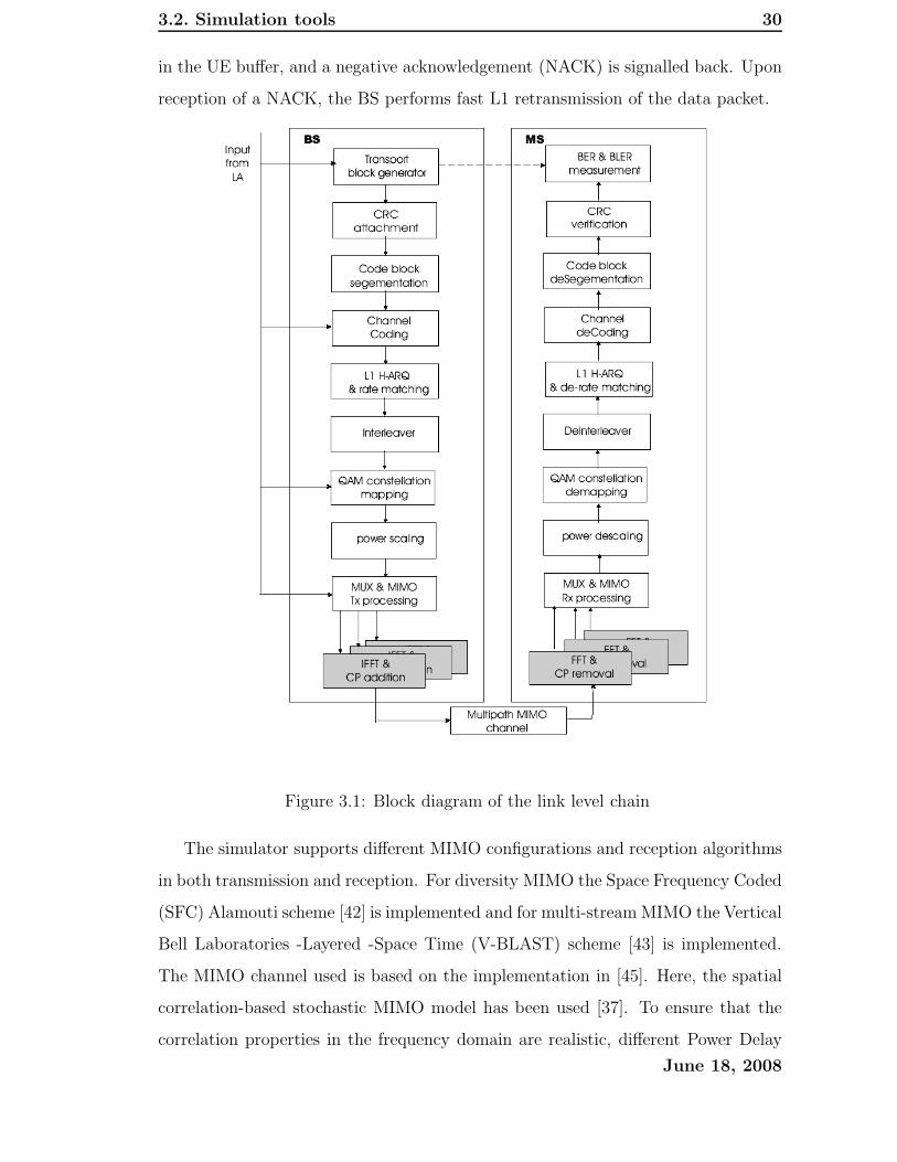
3.2. Simulation tools 30
in the UE buffer, and a negative acknowledgement (NACK) is signalled back. Upon
reception of a NACK, the BS performs fast L1 retransmission of the data packet.
Figure 3.1: Block diagram of the link level chain
The simulator supports different MIMO configurations and reception algorithms
in both transmission and reception. For diversity MIMO the Space Frequency Coded
(SFC) Alamouti scheme [42] is implemented and for multi-stream MIMO the Vertical
Bell Laboratories -Layered -Space Time (V-BLAST) scheme [43] is implemented.
The MIMO channel used is based on the implementation in [45]. Here, the spatial
correlation-based stochastic MIMO model has been used [37]. To ensure that the
correlation properties in the frequency domain are realistic, different Power Delay
June 18, 2008

3.2. Simulation tools 31
Profiles (PDP) from COST 259 [46] and ITU-R M.1225 [16] will be used in this
study. Antennas are assumed to be uncorrelated. Note that for the further chapters
of this thesis only the SISO antenna configuration will be used. Different channel
estimation algorithms, as well as pilot schemes are also implemented and will be
further elaborated in chapters 6 and 7. The PER and spectral efficiency results
provided by this simulator will be given for different Sinal to Noise Ratio (SNR)
values, where SNR is defined as the ratio between the received signal power and the
noise power. No errors are assumed in the transmission of ACK/NACK messages.
Further, the channel estimation is assumed to be ideal for the baseline results. To
allow for processing and propagation delays, the retransmission scheme is based on
the stop and wait (SAW).
3.2.2 Uncoded OFDM simulator
The second simulator was developed with the intention of obtaining results at a
highly reduced simulation time. It closely follows the block diagram of figure 2.4
where all modules related to channel coding are removed, namely: TFRC, CRC
attachment, HARQ, Interleaving, Link Adaptation. Also the MIMO module is
removed as not needed for the study. As the data of consecutive transmitted OFDM
symbols, is uncorrelated, the channel model is assumed to be uncorrelated block
fading. By this is meant that for each transmitted OFDM symbol a new CIR with
uncorrelated Rayleigh taps is generated. This setup allows the simulation time to
be strongly reduced for generation of uncoded Bit Error Rate (BER) and Mean
Squared Error (MSE) results.
The advantages of this simulator are its large flexibility in parameter settings
allowing to go beyond the settings of specified for LTE and its increased simula-
tion speed as results converge quickly because of the uncorrelated block fading.
Thereby more investigations for comparative results can be run before making a
wiser selection of parameter settings and algorithms to be run in the L1-EUTRA
link simulator.
June 18, 2008
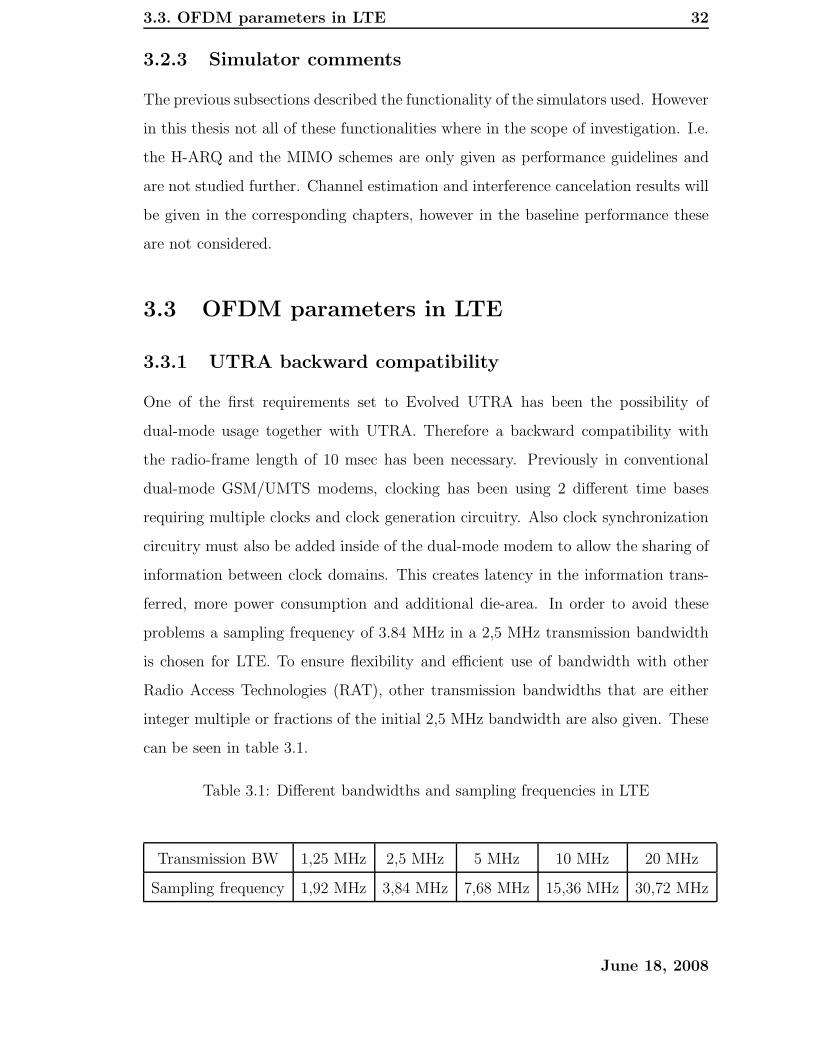
3.3. OFDM parameters in LTE 32
3.2.3 Simulator comments
The previous subsections described the functionality of the simulators used. However
in this thesis not all of these functionalities where in the scope of investigation. I.e.
the H-ARQ and the MIMO schemes are only given as performance guidelines and
are not studied further. Channel estimation and interference cancelation results will
be given in the corresponding chapters, however in the baseline performance these
are not considered.
3.3 OFDM parameters in LTE
3.3.1 UTRA backward compatibility
One of the first requirements set to Evolved UTRA has been the possibility of
dual-mode usage together with UTRA. Therefore a backward compatibility with
the radio-frame length of 10 msec has been necessary. Previously in conventional
dual-mode GSM/UMTS modems, clocking has been using 2 different time bases
requiring multiple clocks and clock generation circuitry. Also clock synchronization
circuitry must also be added inside of the dual-mode modem to allow the sharing of
information between clock domains. This creates latency in the information trans-
ferred, more power consumption and additional die-area. In order to avoid these
problems a sampling frequency of 3.84 MHz in a 2,5 MHz transmission bandwidth
is chosen for LTE. To ensure flexibility and efficient use of bandwidth with other
Radio Access Technologies (RAT), other transmission bandwidths that are either
integer multiple or fractions of the initial 2,5 MHz bandwidth are also given. These
can be seen in table 3.1.
Table 3.1: Different bandwidths and sampling frequencies in LTE
Transmission BW 1,25 MHz 2,5 MHz 5 MHz 10 MHz 20 MHz
Sampling frequency 1,92 MHz 3,84 MHz 7,68 MHz 15,36 MHz 30,72 MHz
June 18, 2008
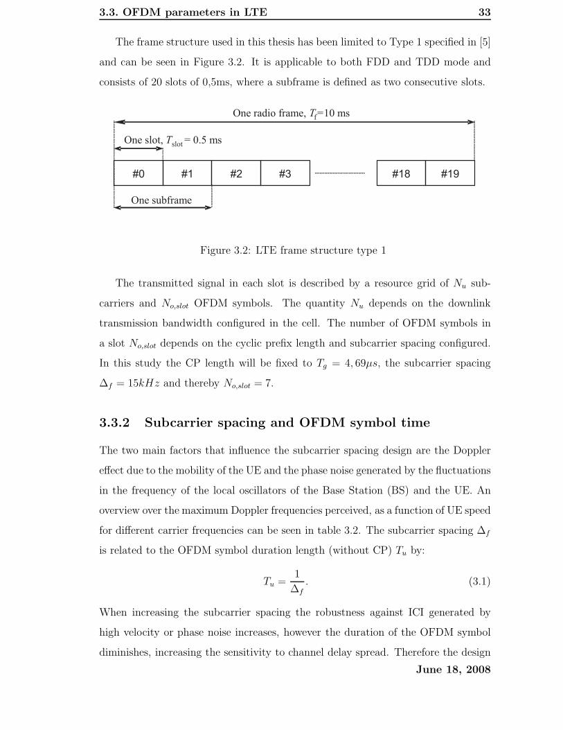
3.3. OFDM parameters in LTE 33
The frame structure used in this thesis has been limited to Type 1 specified in [5]
and can be seen in Figure 3.2. It is applicable to both FDD and TDD mode and
consists of 20 slots of 0,5ms, where a subframe is defined as two consecutive slots.
#0 #1 #2 #3 #19
One slot, Tslot= 0.5 ms
One radio frame, Tf=10 ms
#18
One subframe
Figure 3.2: LTE frame structure type 1
The transmitted signal in each slot is described by a resource grid of Nu sub-
carriers and No,slot OFDM symbols. The quantity Nu depends on the downlink
transmission bandwidth configured in the cell. The number of OFDM symbols in
a slot No,slot depends on the cyclic prefix length and subcarrier spacing configured.
In this study the CP length will be fixed to Tg = 4, 69µs, the subcarrier spacing
∆f = 15kHz and thereby No,slot = 7.
3.3.2 Subcarrier spacing and OFDM symbol time
The two main factors that influence the subcarrier spacing design are the Doppler
effect due to the mobility of the UE and the phase noise generated by the fluctuations
in the frequency of the local oscillators of the Base Station (BS) and the UE. An
overview over the maximum Doppler frequencies perceived, as a function of UE speed
for different carrier frequencies can be seen in table 3.2. The subcarrier spacing ∆f
is related to the OFDM symbol duration length (without CP) Tu by:
Tu =1
∆f
. (3.1)
When increasing the subcarrier spacing the robustness against ICI generated by
high velocity or phase noise increases, however the duration of the OFDM symbol
diminishes, increasing the sensitivity to channel delay spread. Therefore the design
June 18, 2008
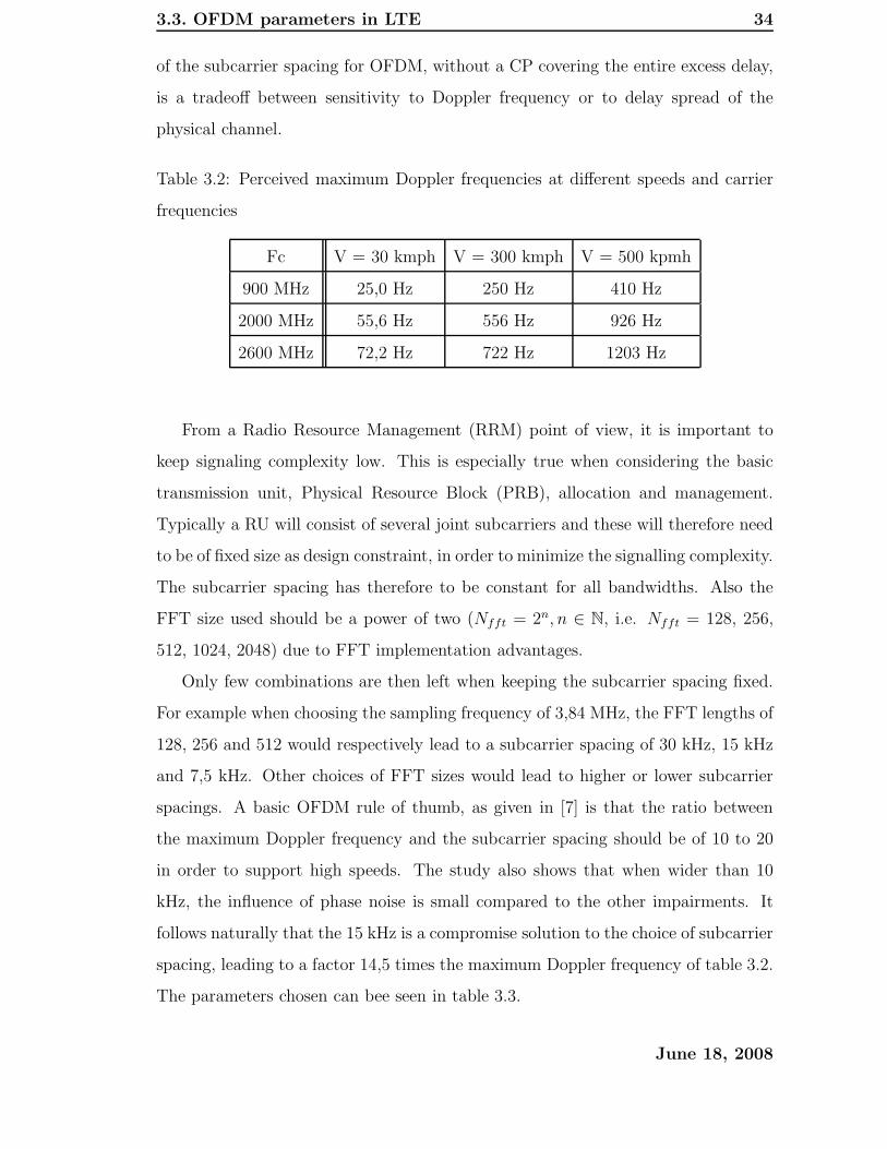
3.3. OFDM parameters in LTE 34
of the subcarrier spacing for OFDM, without a CP covering the entire excess delay,
is a tradeoff between sensitivity to Doppler frequency or to delay spread of the
physical channel.
Table 3.2: Perceived maximum Doppler frequencies at different speeds and carrier
frequencies
Fc V = 30 kmph V = 300 kmph V = 500 kpmh
900 MHz 25,0 Hz 250 Hz 410 Hz
2000 MHz 55,6 Hz 556 Hz 926 Hz
2600 MHz 72,2 Hz 722 Hz 1203 Hz
From a Radio Resource Management (RRM) point of view, it is important to
keep signaling complexity low. This is especially true when considering the basic
transmission unit, Physical Resource Block (PRB), allocation and management.
Typically a RU will consist of several joint subcarriers and these will therefore need
to be of fixed size as design constraint, in order to minimize the signalling complexity.
The subcarrier spacing has therefore to be constant for all bandwidths. Also the
FFT size used should be a power of two (Nfft = 2n, n ∈ N, i.e. Nfft = 128, 256,
512, 1024, 2048) due to FFT implementation advantages.
Only few combinations are then left when keeping the subcarrier spacing fixed.
For example when choosing the sampling frequency of 3,84 MHz, the FFT lengths of
128, 256 and 512 would respectively lead to a subcarrier spacing of 30 kHz, 15 kHz
and 7,5 kHz. Other choices of FFT sizes would lead to higher or lower subcarrier
spacings. A basic OFDM rule of thumb, as given in [7] is that the ratio between
the maximum Doppler frequency and the subcarrier spacing should be of 10 to 20
in order to support high speeds. The study also shows that when wider than 10
kHz, the influence of phase noise is small compared to the other impairments. It
follows naturally that the 15 kHz is a compromise solution to the choice of subcarrier
spacing, leading to a factor 14,5 times the maximum Doppler frequency of table 3.2.
The parameters chosen can bee seen in table 3.3.
June 18, 2008

3.4. Baseline performance 35
Table 3.3: FFT sizes for the different bandwidths
Transmission BW 1,25 MHz 2,5 MHz 5 MHz 10 MHz 20 MHz
FFT size 128 256 512 1024 2048
Subcarrier spacing 15 kHz
3.4 Baseline performance
3.4.1 Achievable peak rates in DL LTE
In the following, we propose to give a realistic estimate of the achievable maxi-
mum peak rates, just from reading the LTE specifications and assuming optimal
transmission conditions. At the moment of writing this Ph.D. thesis, the standard-
ization process is still ongoing and some of the parameters and settings given in
the following might vary from the ones that will be used ultimately. In the 3GPP
TS36 series, the LTE physical layer is specified. LTE proposes a flexible bandwidth
usage (supporting 1.25, 2.5, 5, 10 and 20 MHz) leading to a scalable number of
used subcarriers Nu ∈ {76, 151, 301, 601, 1201}. In the case of the generic down-
link frame structure proposed in TS36.211 [5], where a subframe is of duration 1
ms and contains 14 OFDM symbols, the number of OFDM symbols per second
No,sec is then 14000. A high spectral efficiency is then obtained with the use of
MIMO schemes and especially spatial multiplexing where the maximum number
of streams Nstream ∈ {1, 2, 4} mainly depends on the available antenna configura-
tion and antenna correlation. The high peak rates will then be achieved with the
20MHz bandwidth and by combining the mentioned techniques with higher order
modulation such as QPSK, 16QAM and 64QAM where the number of bits per data
symbols is Nmod ∈ {2, 4, 6}. The transmitted data is encoded with a Turbo encoder
which leads to additional redundancy. A subset of suggested ECRs is given by
Oecr ∈ { 1/6, 1/3, 1/2, 2/3, 3/4, 4/5, 5/6}. Practical issues such synchronization
and channel estimation require presence of pilot data giving a pilot loss factor of
Opilot ∈ {0.9524 0.9048 0.8571} corresponding respectively to a loss of 4.76 %, 9.52
% and 14.29 %. This pilot loss depends on the different MIMO and MBMS settings.
June 18, 2008

3.4. Baseline performance 36
Finally a protocol signalling and together with CP loss Osig = 0.70 of 30% is also
considered.
QPSK 16QAM 64QAM0
50
100
150
200
250
Est
imat
ed m
axim
um th
roug
hput
(M
bit/s
ec)
1 x 12 x 24 x 4
Figure 3.3: Maximum deliverable throughput in LTE for different physical layer
configurations
The throughput can then be expressed as:
Throughput = (No,sec ·Nu · Nmod · Nstream) · Opilot · Oecr · Osig. (3.2)
The different estimated maximum achievable throughputs in LTE are given in Figure
3.3 for a 20MHz bandwidth, for three MIMO scenarios and given an efficient code
rate of 5/6. These numbers should be seen as the ”best case” feasible scenario. By
”best case” is meant the highest effective code rate with a PER of 0, and by feasible
is meant calculations including most overhead that is present in both physical layer
and signalling. From the observed numbers it can be concluded that the LTE peak
rate objectives of 100 Mbit per second will only be achieved with multistream MIMO
combined with higher order modulation (at least 16QAM).
June 18, 2008

3.4. Baseline performance 37
3.4.2 Baseline performance
Now that the achievable peak rates in DL LTE have been described, some baseline
spectral efficiency results will be given. The L1-EUTRA simulator is used for this
performance analysis. The parameter settings used are the ones from section 3.3
for a 10 MHz scenario. No overhead due to pilot symbols is considered here as the
degradation due to channel estimation is not studied in the baseline performance.
This degradation will however be largely studied in later chapters. The set of Mod-
ulation and Code Schemes (MCS) chosen is given on table 3.4. The turbo decoder
implementation has been verified against results in [14]. The uncoded BER perfor-
mance of the link simulator has also been verified for different modulation formats.
Throughput results have also been compared to the ones from other companies in
appendix B.
Table 3.4: Used set of MCS
Modulation ECR
QPSK 1/6, 1/3, 1/2, 2/3
16QAM 1/2, 2/3, 3/4
64QAM 3/4, 4/5
In figure 3.4, the spectral efficiency, defined as useful throughput over bandwidth,
of different modulation and code sets without HARQ, in a SISO antenna configura-
tion is plotted versus SNR. The bandwidth is set to 10 MHz and the channel model
is the Typical Urban [46].
The spectral efficiency versus SNR when using HARQ is shown in figure 3.5 for 3
MCS using Incremental Redundancy (IR). Including HARQ increases performance
for all SNRs except when the PER is null. In this case there is no gain to achieve,
as no retransmissions are needed. The individual curves without HARQ have the
characteristic steep slope due to the Turbo Codes employed. When using HARQ
the BLER degradation is more gradual and the classical staircase curve is observed
with a correspondence between the number of average packet transmissions and the
different steps.
June 18, 2008

3.4. Baseline performance 38
−10 −5 0 5 10 15 20 25 300
0.5
1
1.5
2
2.5
3
3.5
4
4.5
SNR (dB)
Spe
ctra
l Effi
cien
cy (
bits
/s/H
z)
QPSK 0.17QPSK 0.33QPSK 0.50QPSK 0.6716QAM 0.5016QAM 0.6716QAM 0.7564QAM 0.6764QAM 0.80
Figure 3.4: without HARQ
−10 −5 0 5 10 15 20 25 300
0.5
1
1.5
2
2.5
3
3.5
4
4.5
SNR (dB)
Spe
ctra
l Effi
cien
cy (
bits
/s/H
z)
QPSK 0.67 HARQ16QAM 0.67 HARQ64QAM 0.80 HARQQPSK 0.67 no HARQ16QAM 0.67 no HARQ64QAM 0.80 no HARQ
Figure 3.5: HARQ vs. no HARQ
−10 0 10 20 30 400
1
2
3
4
5
6
7
8
9
SNR (dB)
Spe
ctra
l Effi
cien
cy (
b/s/
Hz)
SISO (1x1)SFC (2x2)BLAST (2x2)
Figure 3.6: Maximal Spectral Efficiency for different MIMO schemes without
HARQ in a 10 MHz bandwidth
In Figure 3.6, the spectral efficiency for the different antenna configuration and
reference MIMO schemes are shown for comparison. Three performance curves are
included. All curves represent the maximal achievable performance from adapting
to the best MCS set for a given average SNR. The first curve represents the SISO
June 18, 2008

3.5. Conclusion 39
case from figure 3.4. The second one is based on single data stream Alamouti [42]
SFC scheme with a 2 by 2 antenna configuration. The third curve represents a dual
stream, 2 by 2 antenna configuration, BLAST scheme. At SNR below 17dB, both
dual antenna schemes have similar performance with a gain of 5-7 dB over the SISO
performance. At SNR above 17dB the SFC performance is saturated and converges
towards the one from SISO. The BLAST performance however, gains from the dual
stream transmission where the spectral efficiency is doubled at SNR above 28 dB,
compared to the two other single stream schemes performance curves.
3.5 Conclusion
In this chapter the simulator context and LTE baseline performance have been
presented. The two simulators that will be used for the rest of this thesis have been
described. These are the L1-EUTRA link simulator for DL LTE and the uncoded
OFDM simulator. The L1-EUTRA was developed to generate accurate link results
according to 3GPP requirements and was verified by comparing performance against
official results from other companies. Thereby the obtained SISO simulation chain
results have been verified. The uncoded OFDM simulator only generates BER, MSE
and SINR results, but simulation time is greatly reduced as no FEC is included and
the simulated radio channel is based on block fading.
The physical layer parameters adopted for DL LTE have been described and
the reasoning behind their choice and design has been explained. With these pa-
rameters, baseline performance for 10 MHz was outlined for key reference scenarios.
First the maximum achievable peak rates were given for different antenna configura-
tions and modulation schemes (QPSK, 16QAM and 64QAM ). In the same manner,
spectral efficiency results for different SNR values were presented showing the ad-
vantages of using HARQ and MIMO schemes. More specifically the 2 by 2 antenna
Alamouti SFC and BLAST schemes advantages against simple 1 by 1 antenna SISO
configuration were drawn to light.
For the rest of this thesis the investigations carried out will however be restricted
to the SISO 1 by 1 antenna scenario without the use of HARQ.
June 18, 2008

Chapter 4
On Cyclic Prefix Length
4.1 Introduction
A CP is generally inserted in OFDM transmission. It is an additional redundant
guard period that efficiently combats interference resulting from the multipath na-
ture of the physical channel. If the CP length is larger than the length of the
Maximum Excess Delay (MED), all multipath energy resulting from delayed ver-
sions of the signal is constructively recovered [20] [21]. The CP has no influence on
the interference resulting from mobility and the resulting Doppler shift [22]. There-
fore, arbitrarily, the Doppler spectrum is considered flat in this subsection. The
introduction of CP has the drawback of reducing the overall system capacity in an
irreversible manner. This reduction can be expressed through the Spectral Efficiency
Loss (SEL): SEL = Tg
Tofdm, with Tg being the CP length, Tu the useful symbol length
and Tofdm = Tg + Tu the total OFDM symbol length. It can be see that the SEL
does not only depend on Tg but also on Tu . If Tg is fixed, the SEL diminishes when
Tu is increased. During this study Tu will be fixed to a few chosen values inspired
from previous studies [53], [54] for generic results and the LTE parameters for more
specific LTE results. On the other hand, as CP covers more and more of the PDP
length it reduces the SINR, thus enhancing the overall BLER performance of the
system. The other advantage when the CP length is larger than the MED is that
interference free reception can be achieved with a Single Tap Equalizer (STE) [55].
From a complexity point of view this STE has interesting properties and is there-
40

4.2. SINR evaluation 41
fore adopted in the following. System level CP length studies have previously been
conducted but without focusing precisely on variation of PDP. In [56] for instance,
CP length was studied in connection with synchronization.
Efficient adaptive CP length has recently been proposed by Lim [57] . The
drawback of such a solution is increased signalling overhead. In this chapter we
conduct a study giving insight on the choice of an optimal CP length. We also
evaluate and propose different fixed CP lengths and compare them to the proposed
values of LTE in [5]. In section 4.2 an analytical method for evaluating SINR in
OFDM is given leading to an evaluation of CP length in section 4.3. Finally we
conclude in 4.4.
4.2 SINR evaluation
In the following, an analytical method for evaluating SINR, inspired from [22] and
[56], is presented. This method gives an intuitive understanding of the effects of Tg,
Tu, Tofdm, the PDP and SNR on the received SINR. The method is then verified by
a statistical evaluation.
A general SINR formulation is given by:
SINR =Ps
Pi + σ2w
(4.1)
Where Ps is the ”useful” signal power, Pi is the interference power, and σ2w is the
variance of the white gaussian noise. All powers are expressed per subcarrier.
Analytical SINR evaluation
In this section the ”useful” signal and the interference signal are both calculated
from a given PDP and a weighting function called ”bias function” seen on Figure
4.1. This function was first used in [22] and extended to use timing offset in [56].
The synchronicity assumption leads to the following definition:
C(τ) =
0, τ < 0
1, 0 ≤ τ < Tg
Tu−(τ−Tg)Tu
, Tg ≤ τ < Tofdm
0, Tofdm ≤ τ
June 18, 2008
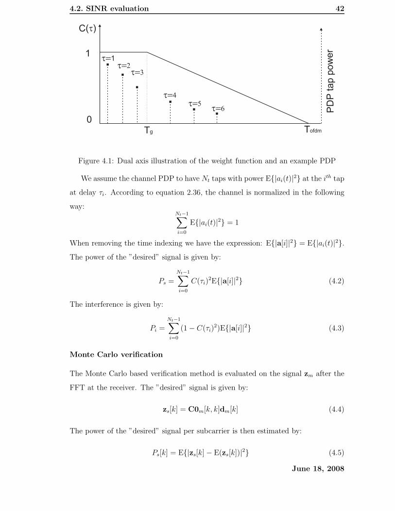
4.2. SINR evaluation 42
0
1
Tg Tofdm
PD
Pta
pp
ow
er
C( )t
t=1t=2
t=3
t=4
t=5t=6
Figure 4.1: Dual axis illustration of the weight function and an example PDP
We assume the channel PDP to have Nt taps with power E{|ai(t)|2} at the ith tap
at delay τi. According to equation 2.36, the channel is normalized in the following
way:Nt−1∑
i=0
E{|ai(t)|2} = 1
When removing the time indexing we have the expression: E{|a[i]|2} = E{|ai(t)|2}.
The power of the ”desired” signal is given by:
Ps =
Nt−1∑
i=0
C(τi)2E{|a[i]|2} (4.2)
The interference is given by:
Pi =Nt−1∑
i=0
(1 − C(τi)2)E{|a[i]|2} (4.3)
Monte Carlo verification
The Monte Carlo based verification method is evaluated on the signal zm after the
FFT at the receiver. The ”desired” signal is given by:
zs[k] = C0m[k, k]dm[k] (4.4)
The power of the ”desired” signal per subcarrier is then estimated by:
Ps[k] = E{|zs[k] − E(zs[k])|2} (4.5)
June 18, 2008
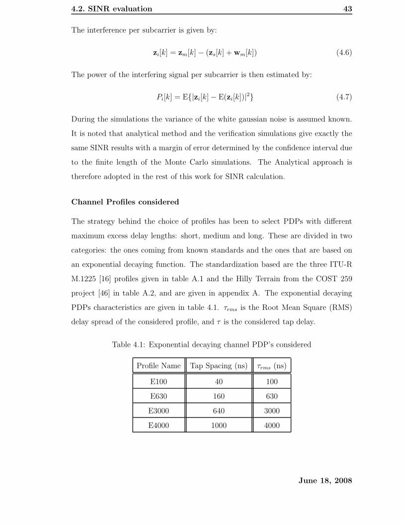
4.2. SINR evaluation 43
The interference per subcarrier is given by:
zi[k] = zm[k] − (zs[k] + wm[k]) (4.6)
The power of the interfering signal per subcarrier is then estimated by:
Pi[k] = E{|zi[k] − E(zi[k])|2} (4.7)
During the simulations the variance of the white gaussian noise is assumed known.
It is noted that analytical method and the verification simulations give exactly the
same SINR results with a margin of error determined by the confidence interval due
to the finite length of the Monte Carlo simulations. The Analytical approach is
therefore adopted in the rest of this work for SINR calculation.
Channel Profiles considered
The strategy behind the choice of profiles has been to select PDPs with different
maximum excess delay lengths: short, medium and long. These are divided in two
categories: the ones coming from known standards and the ones that are based on
an exponential decaying function. The standardization based are the three ITU-R
M.1225 [16] profiles given in table A.1 and the Hilly Terrain from the COST 259
project [46] in table A.2, and are given in appendix A. The exponential decaying
PDPs characteristics are given in table 4.1. τrms is the Root Mean Square (RMS)
delay spread of the considered profile, and τ is the considered tap delay.
Table 4.1: Exponential decaying channel PDP’s considered
Profile Name Tap Spacing (ns) τrms (ns)
E100 40 100
E630 160 630
E3000 640 3000
E4000 1000 4000
June 18, 2008
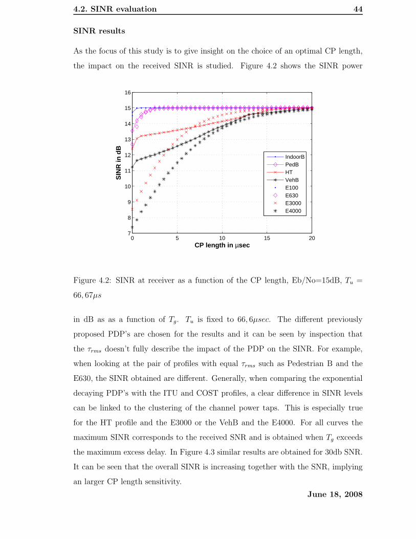
4.2. SINR evaluation 44
SINR results
As the focus of this study is to give insight on the choice of an optimal CP length,
the impact on the received SINR is studied. Figure 4.2 shows the SINR power
0 5 10 15 207
8
9
10
11
12
13
14
15
16
CP length in µsec
SIN
R in
dB
IndoorBPedBHTVehBE100E630E3000E4000
Figure 4.2: SINR at receiver as a function of the CP length, Eb/No=15dB, Tu =
66, 67µs
in dB as as a function of Tg. Tu is fixed to 66, 6µsec. The different previously
proposed PDP’s are chosen for the results and it can be seen by inspection that
the τrms doesn’t fully describe the impact of the PDP on the SINR. For example,
when looking at the pair of profiles with equal τrms such as Pedestrian B and the
E630, the SINR obtained are different. Generally, when comparing the exponential
decaying PDP’s with the ITU and COST profiles, a clear difference in SINR levels
can be linked to the clustering of the channel power taps. This is especially true
for the HT profile and the E3000 or the VehB and the E4000. For all curves the
maximum SINR corresponds to the received SNR and is obtained when Tg exceeds
the maximum excess delay. In Figure 4.3 similar results are obtained for 30db SNR.
It can be seen that the overall SINR is increasing together with the SNR, implying
an larger CP length sensitivity.
June 18, 2008
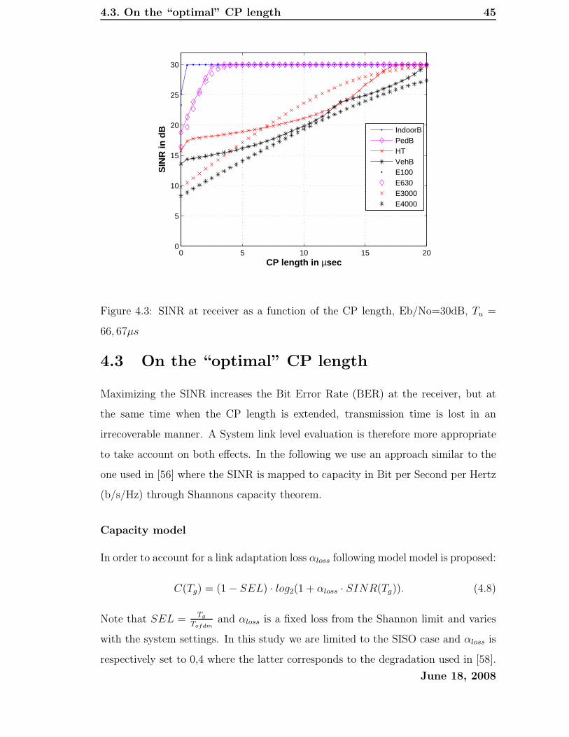
4.3. On the “optimal” CP length 45
0 5 10 15 200
5
10
15
20
25
30
CP length in µsec
SIN
R in
dB IndoorB
PedBHTVehBE100E630E3000E4000
Figure 4.3: SINR at receiver as a function of the CP length, Eb/No=30dB, Tu =
66, 67µs
4.3 On the “optimal” CP length
Maximizing the SINR increases the Bit Error Rate (BER) at the receiver, but at
the same time when the CP length is extended, transmission time is lost in an
irrecoverable manner. A System link level evaluation is therefore more appropriate
to take account on both effects. In the following we use an approach similar to the
one used in [56] where the SINR is mapped to capacity in Bit per Second per Hertz
(b/s/Hz) through Shannons capacity theorem.
Capacity model
In order to account for a link adaptation loss αloss following model model is proposed:
C(Tg) = (1 − SEL) · log2(1 + αloss · SINR(Tg)). (4.8)
Note that SEL = Tg
Tofdmand αloss is a fixed loss from the Shannon limit and varies
with the system settings. In this study we are limited to the SISO case and αloss is
respectively set to 0,4 where the latter corresponds to the degradation used in [58].
June 18, 2008

4.3. On the “optimal” CP length 46
Simulation results
0 5 10 15 200
1
2
3
4
5
6
7
8
CP length in µsec
Cap
acity
(b/
s/H
z)
26 dB21 dB16 dB11 dB6 dB1 dB
Figure 4.4: Influence of the received SNR on CP length. Capacity for different
received signal powers, PDP= PedB Tu = 66, 67µs
The SINR defined previously in equation 4.1 depends on the ”desired” SNR at
the receiver. Note that the SNR is equal to the SINR when the CP length is larger
than the maximum excess delay of the CIR. The impact of the SNR is studied in
Figure 4.4. It is observed that the receiver is more sensitive to the CP length at
high SNR, whereas at low SNR its impact is almost neglegible. I.e. at 26 dB there
is a difference of 2,2 b/s/Hz for Tu varying between 0 an 2,5µs, whereas at 1 dB the
variation is less than 0,1 b/s/Hz in the same interval. Therefore in the following
only a high midrange SNR value of 16dB is considered.
The length of the ”useful” OFDM symbol Tu is studied in Figure 4.5 where the
capacity versus the CP length is plotted for Tu varying from 10µs to 160 µs and the
PDP is PedB. It is noted that Tu only has little influence on the optimal CP length.
However the longer Tu, the less sensitive the capacity is to a non optimal CP length
(that is too short or too long). I.e. if Tg = 8µs then with Tu = 160µs the capacity
is only reduced by 0,2 b/s/Hz from the maximum achievable performance. On the
June 18, 2008

4.3. On the “optimal” CP length 47
0 2 4 6 8 102
2.5
3
3.5
4
4.5
5
CP length in µsec
Cap
acity
(b/
s/H
z)
160 µs80 µs60 µs40 µs20 µs10 µs
Figure 4.5: Influence of useful OFDM symbol length Tu on CP length Tg. Capacity
for different received signal powers, PDP= PedB, Eb/No=16dB
other hand, with Tu = 10µs the loss would be more than 1,0 b/s/Hz.
In Figure 4.6, the four exponentially decaying PDPs of table 4.1 are plotted. It
is noted that the optimal CP length increases as τrms increases. This result has
often been used as a design guideline in common literature. Yet when comparing
HT [46] and VehB [16] of respectively τrms of 3000 and 4000 ns with their exponential
decaying counterparts at same τrms , it is noted that the optimal CP length can
significantly vary from profile to profile. I.e. for the HT PDP, the optimum Tg is
1,1µs, but for the E3000 PDP it is 9,8 µs. Hence linear dependency is not always
true between optimal CP length and τrms and the entire PDP must be considered
for proper evaluation.
Discussion
In order to avoid system signaling overhead to control a variable CP length, one
single constant CP value is preferable. This length should give the best average
performance. The highest capacity is achieved with a 1 path PDP and no CP.
June 18, 2008
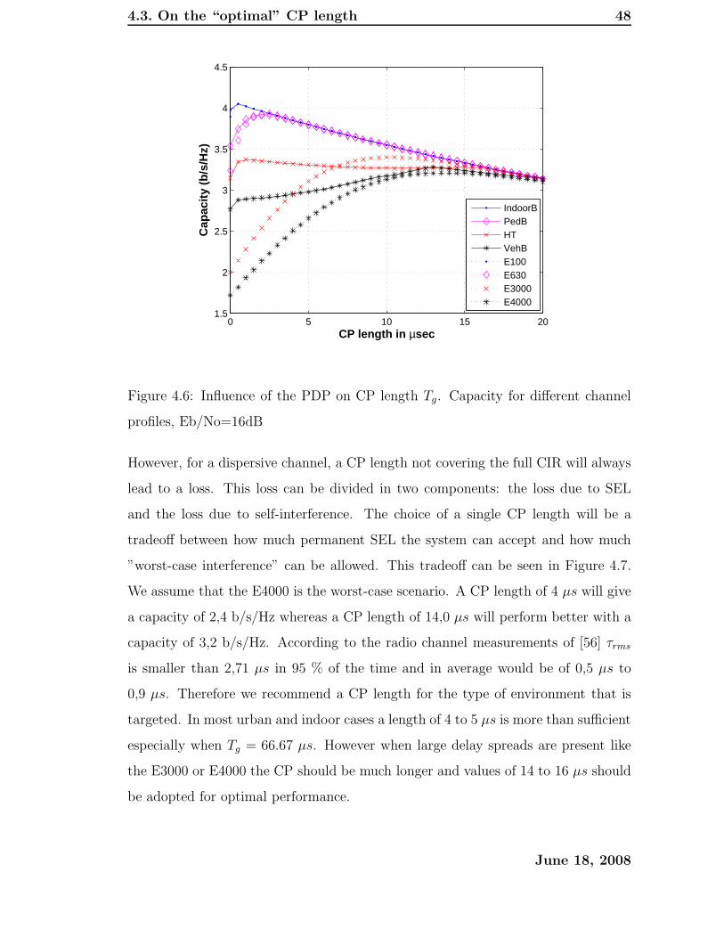
4.3. On the “optimal” CP length 48
0 5 10 15 201.5
2
2.5
3
3.5
4
4.5
CP length in µsec
Cap
acity
(b/
s/H
z)IndoorBPedBHTVehBE100E630E3000E4000
Figure 4.6: Influence of the PDP on CP length Tg. Capacity for different channel
profiles, Eb/No=16dB
However, for a dispersive channel, a CP length not covering the full CIR will always
lead to a loss. This loss can be divided in two components: the loss due to SEL
and the loss due to self-interference. The choice of a single CP length will be a
tradeoff between how much permanent SEL the system can accept and how much
”worst-case interference” can be allowed. This tradeoff can be seen in Figure 4.7.
We assume that the E4000 is the worst-case scenario. A CP length of 4 µs will give
a capacity of 2,4 b/s/Hz whereas a CP length of 14,0 µs will perform better with a
capacity of 3,2 b/s/Hz. According to the radio channel measurements of [56] τrms
is smaller than 2,71 µs in 95 % of the time and in average would be of 0,5 µs to
0,9 µs. Therefore we recommend a CP length for the type of environment that is
targeted. In most urban and indoor cases a length of 4 to 5 µs is more than sufficient
especially when Tg = 66.67 µs. However when large delay spreads are present like
the E3000 or E4000 the CP should be much longer and values of 14 to 16 µs should
be adopted for optimal performance.
June 18, 2008

4.4. Conclusion 49
2 4 6 8 10 12 14 16 18 200
1
2
3
4
5
6
CP length in µs
Cap
acity
(b/
s/H
z)
Worst Case performanceLoss due to Interferenceloss due to SEL
Figure 4.7: On the efficiency of the CP to cope with multipathTg. , Eb/No=16dB,
Tu = 66, 67µs, PDP= E4000
4.4 Conclusion
In this chapter we have studied the influence of CP length on SISO OFDM system
capacity with LTE based parameters, when using a single tap equalizer in the re-
ceiver. The results showed that if only one CP length is to be chosen, then a good
tradeoff value would be in the range 4 to 5 µs as high SNRs are mostly observed in
Urban areas and the PDP lengths are not to large. This would still give relatively
acceptable performance in long delay areas as the expected SNRs are lowered. Two
different SINR models were proposed and proved to give same results. The influence
of different parameters on the CP length design were analyzed.
First, it was shown in the study that the received SNR increased the sensitivity
of the Capacity to the CP length. This can be interpreted as: Tx power and other
cell interference affect the capacity. A higher Tx power will increase the sensitivity
to a correct CP length and thereby increase the CP length. On the other hand,
higher other cell interference will decrease the sensitivity to CP and its length could
be reduced.
June 18, 2008
4.4. Conclusion 50
Secondly, it was shown that the duration of the useful OFDM symbol didn’t
impact the optimal CP length significantly. However it impacted the capacity loss
due to a CP being too long or too short. Therefore the useful OFDM symbol should
be as long as the system design allows.
In a third step, the RMS delay spread of a PDP turns out not to be a sufficient
statistic to determine the optimal CP length. The whole PDP of the channel shall
be considered. Large variations of optimal CP length can be observed for PDPs
having equal RMS delay spread.
More areas remain for future study. Capacity analysis based on SINR analysis
for different channel environments, was used as quality measure to determine the
optimal CP length. A fixed loss from the shannon limit was adopted, yet larger and
more detailed link simulation study could increase the accuracy of the results. Also
the effect of MIMO techniques is also an important topic for further investigation
in a LTE context. Finally interference cancelation techniques should be considered.
Some of these techniques are treated in chapter 8 of this thesis.
June 18, 2008
Chapter 5
Channel Estimation in OFDM and
LTE
5.1 Introduction
In the previous chapters the OFDM signal has been modeled at different levels
and system parameter design has been studied. The simulation results assumed
the Channel Transfer Function (CTF) to be known to the receiver for equalization.
Thereby the results have been used for best-case performance evaluation. When
more realistic results are desired and receiver algorithm design is considered, chan-
nel estimation needs to be studied. In a classical CP-OFDM receiver with coherent
detection, the CTF needs to be estimated in order to compensate for channel dis-
tortion prior to demodulation. The accuracy of the estimator influences greatly the
total system performance. Particularly the sensitivity is increased with higher order
modulation schemes or higher SNR’s. Channel estimation techniques can be sepa-
rated in the ones operating on the frequency response of the OFDM symbol (signal
after receiver FFT) and the ones employing time domain correlation algorithms.
The latter will not be the scope of the study in this thesis. Among the algorithms
operating on the spectrum of the received OFDM symbol, different strategies have
been studied in literature.
Pilot based Channel Estimation (PACE), the most common technique, is based
on Pilot Symbol-Assisted Modulation (PSAM) where known information to the
51

5.2. The physical radio channel model 52
transmitter and receiver is inserted at given subcarriers. For each received pilot
subcarrier the corresponding CTF value is estimated. Then, the CTF estimate for
the information-carrying subcarriers, is derived from these pilot-based CTF esti-
mates by means of interpolation between them such as [63], [66], [72], [73], [74]
and [75].
Decision Directed Channel Estimation (DDCE) techniques, such as the ones
described by Hanzo, in [26] are based on the concept of generating an initial a
posteriori least-squares CTF estimate of remodulated subcarrier data symbols. This
estimate is then enhanced through signal processing such as 1-D Minimum Mean
Square Error (MMSE) [67], [68] or 2-D MMSE [78] estimator to give an improved
a posteriori CTF estimate. This improved a posteriori CTF estimate is then used
as an a priori channel estimate for the demodulation of the next times lot OFDM
symbol. DDCE techniques such as [86] have been studied using channel predictors
[80]. However such DDCE techniques suffer from some drawbacks that can prevent
them from being used in real life receivers. These are mainly poor compatibility
with frequency hopping schemes, discontinuous transmission and Frequency Domain
Link Adaptation (FDLA). Also and increased complexity is observed compared to
classical linear PACE techniques more especially in the case of MIMO transmission.
Different blind or semi-blind channel estimation techniques have also been stud-
ied as in [90], [91] and [92]. Although the pilot overhead is removed with these
techniques, blind estimation suffer from the need for training period or very high
computational complexity.
In this chapter the channel estimation problematic will be addressed. First
applied to the generic PSAM OFDM scenario; then more specifically elaborated for
LTE.
5.2 The physical radio channel model
5.2.1 General description and considerations
The radio propagation environment experienced by the signal transmitted from a
BS to a MS clearly places the fundamental limitations on the performance of the
June 18, 2008
5.2. The physical radio channel model 53
studied communication system. The radio wave propagation largely depends on the
frequency band of transmission. In the case of LTE the carrier frequency will be
of 2GHz order and therefore characterized as an Ultra High Frequency (UHF) [30].
In that case communication takes place via direct and reflected components of the
radio wave. The wave propagation will be affected by reflections due to both ground,
natural and man-made obstacles. Also diffraction over buildings and hilltops are to
be taken into account.
When looking at received signal strength over time one can distinguish between
long-term and short-term variations. The short term are classically described by
the multipath fading phenomena. The long term variations are described as slow
fading and correspond to gross variations in the terrain profile between BS and MS
over the MS in motion. In this thesis we restrict our work to short-term
variations.
Rayleigh distribution is usually a good approximation for the received signal
envelope. However when a strong direct path is present, the distribution departs
significantly from Rayleigh and can better be described by a Ricean distribution.
In this thesis for simplicity, we restrict our work to Rayleigh fading for
each tap of the multipath CIR.
Apart from the delay domain, signal fading description can also be done in the
frequency domain. Frequency-flat fading is said to exist if all frequency components
within the signal bandwidth behave similarly. Frequency-selective fading is said
to exist if the signal considered occupies a bandwidth larger than the bandwidth
over which spectral components are affected in a similar way. The extent of the
correlation depends on the spread of the delays in time since the phase shift arise
from the excess path delays. The bandwidth over which the spectral components
are affected in a similar way is known as the coherence bandwidth.
A time-frequency characterization of the multipath phenomena is illustrated in
Figure 5.1. The perceived channel is then described by a time varying Channel
Impulse Response (CIR) and by a time varying Channel Transfer Function (CTF).
June 18, 2008
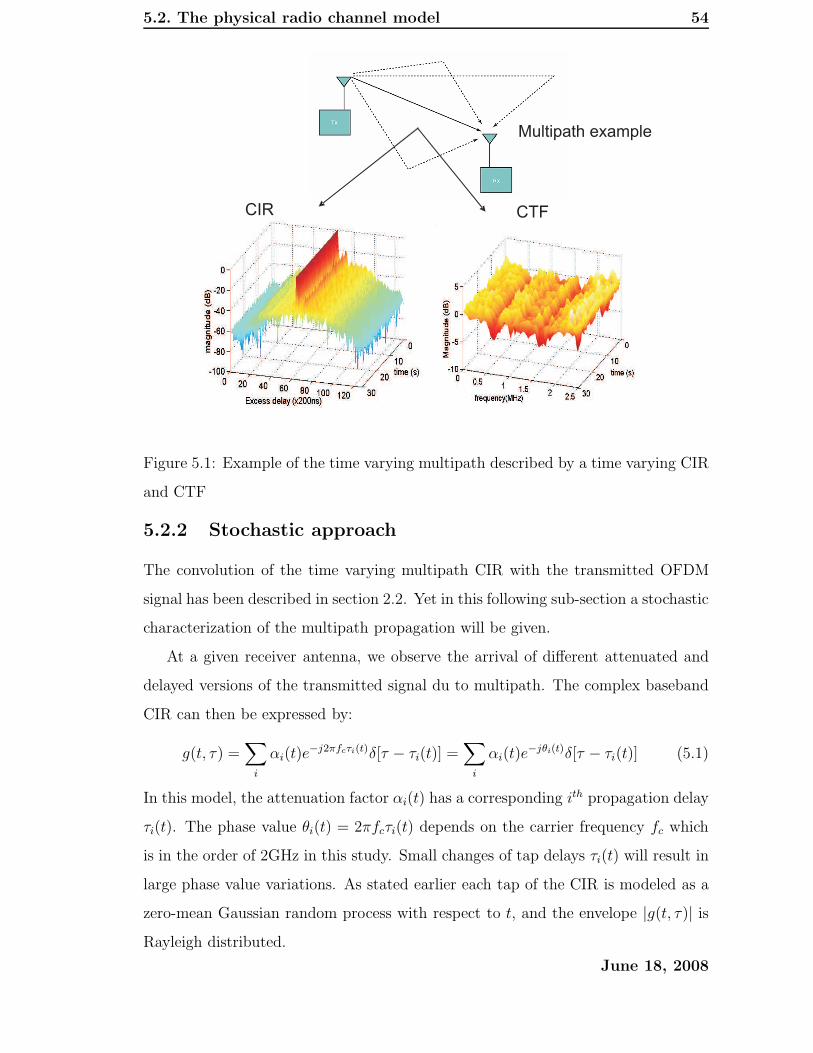
5.2. The physical radio channel model 54
Multipath example
CIR CTF
Figure 5.1: Example of the time varying multipath described by a time varying CIR
and CTF
5.2.2 Stochastic approach
The convolution of the time varying multipath CIR with the transmitted OFDM
signal has been described in section 2.2. Yet in this following sub-section a stochastic
characterization of the multipath propagation will be given.
At a given receiver antenna, we observe the arrival of different attenuated and
delayed versions of the transmitted signal du to multipath. The complex baseband
CIR can then be expressed by:
g(t, τ) =∑
i
αi(t)e−j2πfcτi(t)δ[τ − τi(t)] =
∑
i
αi(t)e−jθi(t)δ[τ − τi(t)] (5.1)
In this model, the attenuation factor αi(t) has a corresponding ith propagation delay
τi(t). The phase value θi(t) = 2πfcτi(t) depends on the carrier frequency fc which
is in the order of 2GHz in this study. Small changes of tap delays τi(t) will result in
large phase value variations. As stated earlier each tap of the CIR is modeled as a
zero-mean Gaussian random process with respect to t, and the envelope |g(t, τ)| is
Rayleigh distributed.
June 18, 2008
5.2. The physical radio channel model 55
The different correlation functions and associated fourier transforms will be given
in the following in order to describe statistically the radio channel as shown in [26].
Auto-Correlation Function (ACF) of the CIR: rg(∆t, τ)
The ACF can be expressed as:
rg(∆t, τ1, τ2) = E{g(t, τ1), g∗(t− ∆t, τ2)} (5.2)
This expression assumes that the CIR process is Wide-Sense-Stationary (WSS) [31],
meaning that the mean value of the process is time invariant and its auto-correlation
is only a function of the time difference ∆t. If the amplitudes and phase shifts of
the different time delays τ1 6= τ2 are uncorrelated, it follows:
rg(∆t, τ1, τ2) = rg(∆t, τ1)δ(τ1 − τ2) (5.3)
The PDP is then given as rg(0, τ) = rg(τ) giving the average power output channel
for a given tap delay τ .
Spaced-time spaced-frequency correlation function: rh(∆t,∆f)
The time variant CTF is denoted by h(t, f) and is obtained by taking the Fourier
transform of the CIR:
h(t, f) =
∫ ∞
−∞g(t, τ)e−j2πfτdτ (5.4)
The auto-correlation function of h(t, f), namely rh(∆t, f1, f2), is then given as the
Fourier transform of the auto-correlation function of the CIR taken with respect to
τ :
rh(∆t, f1, f2) = E{h(t, f1)h∗(t− ∆t, f2)} = Fτ→f{rg(∆t, τ)}
= rh(∆t,∆f),(5.5)
and is also known as the spaced-time spaced-frequency correlation function of the
channel. Given the assumption of WSS it comes that this function is dependent
on ∆f rather than specific frequency values. For ∆t = 0, which corresponds to
considering the CTF’s associated with a specific OFDM symbol, the ACF rh(∆t,∆f)
June 18, 2008
5.3. PACE principles 56
simplifies to rh(0,∆f) = rh(∆f), and which in turn is related to the multipath
intensity profile by:
rh(∆f) = Fτ→∆f{rg(τ)} (5.6)
A definition of the coherence bandwidth (∆f)c of the channel in the range −(∆f)c/2 ≤
∆ ≤ (∆f)c/2 of frequencies over which the CTF exhibits significant correlation, can
be given from this previous relationship. The coherence bandwidth is related to the
multipath spread (maximum excess delay )by:
(∆f)c ≈1
Tmed
(5.7)
Fourier Transform of the CIR’s ACF with respect to the multipath delay
and space-time variables: Sh(fd,∆f)
Further characterization of the channel is done by taking the Fourier transform of
rh(∆t,∆f) with respect to the time difference:
Sh(fd,∆f) = F∆t→fd{rh(∆t,∆f)} (5.8)
In the case of ∆f = 0, this function simplifies to Sh(fd, 0) = Sh(fd), known as
the Doppler power spectrum of the channel. Analogously to the definition of the
coherence bandwidth and the related multipath spread, we can define the Doppler
Spread BD of the channel as the range −BD/2 ≤ fd ≤ BD/2 of frequencies over
which Sh(fd) exhibits significant values. We can express it inverse as the coherence
time as:
tcor ≈1
BD
. (5.9)
5.3 PACE principles
The following will be dealing with Pilot-symbol Aided Channel Estimation (PACE)
in doubly selective physical channels in a downlink OFDM LTE context. Trans-
mitting a radio signal over a multipath fading channel, the receiver signal will have
unknown amplitude and phase variations. When using a classical OFDM receiver as
described in [59], coherent demodulation needs a CTF estimate at each OFDM sym-
bol. Coherent detection of the received signal requires accurate channel estimation
June 18, 2008
5.3. PACE principles 57
to be performed. When dealing with PACE a subset of transmitted subcarriers will
be used as pilot symbols. From the known received pilots, initial estimates of the
CTF at the pilot subcarriers can be obtained. However interpolation between the
initial estimates is required to obtain the full CTF, giving also a channel estimate
at the data subcarrier positions. These pilots will however occupy resources that
could be used for data transmission. Such insertion impacts directly as spectral
efficiency loss of a system. The idea is then to minimize the pilot overhead without
significantly deteriorating the CTF estimate quality. One way of seeing the pilot
spacing in time and frequency direction is a sample grid of the physical channel,
which itself can be more or less selective. The optimum spectral efficiency would
then be achieved by adapting the pilot spacing grid to the perceived physical channel
conditions as shown in [60].
In the following a signal model will first be explained to introduce the initial CTF
estimation at pilot positions. Then the optimum linear interpolator will be presented
in the form of a two dimensional Wiener filter. Finally different pilot constellations
will be discussed and the optimum constellation presented. This section will show
the need for an algorithmic study for practical interpolators as well as pilot spacings
in a LTE context elaborated in chapter 6 and chapter 7.
5.3.1 Signal model
When OFDM is ICI and ISI free it can be modeled as follows. Recalling equation
2.33 the signal after FFT is:
zm[k] = hm[k]dm[k] + wm[k],
with:
m: index for the considered OFDM symbol
k: index for the considered subcarrier
hm[k]: channel transfer function coefficient
dm[k]: transmitted symbol
wm[k]: AWGN contribution
June 18, 2008
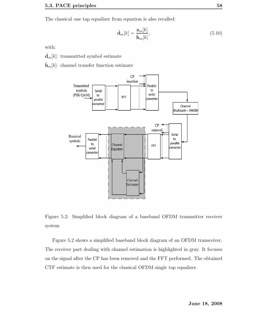
5.3. PACE principles 58
The classical one tap equalizer from equation is also recalled:
dm[k] =zm[k]
hm[k], (5.10)
with:
dm[k]: transmitted symbol estimate
hm[k]: channel transfer function estimate
Figure 5.2: Simplified block diagram of a baseband OFDM transmitter receiver
system
Figure 5.2 shows a simplified baseband block diagram of an OFDM transceiver.
The receiver part dealing with channel estimation is highlighted in gray. It focuses
on the signal after the CP has been removed and the FFT performed. The obtained
CTF estimate is then used for the classical OFDM single tap equalizer.
June 18, 2008

5.3. PACE principles 59
5.3.2 The optimum linear 2D interpolation algorithm
The optimum linear interpolator in the Minimum Mean Square Error (MMSE) sense,
has been derived for PACE by Hoeher in [63] with the 2-dimensional Wiener filter.
This a result also valid in the case when the amount of pilot symbols available for
interpolation is limited [84]. It follows that the channel estimates are computed
from a block of OFDM symbols also called the Channel Estimation Block (CEB).
The pilot of symbols will all contribute with an initial Least Squares (LS) estimate
by:
hCEB,ls[n] = zm[k]dm[k]
, n = ⌈ k∆pf
⌉ + ⌈ m∆pt
⌉ (5.11)
where, ∆pt and ∆pf are the pilot spacing in respectively the time and frequency
direction, hCEB,ls is the LS estimate vector of lengthNp = Npf ·Npt, withNpf andNpt
being the number of pilot subcarriers in respectively frequency and time direction.
Not that the set m, k are chosen only for pilot subcarrier positions. The initial LS
estimates of the channel at the pilot positions then lead to a MMSE estimate of the
CTF expressed by:
hCEB,mmse = CCEBhCEB,ls (5.12)
In this expression illustrated in figure 5.3, hCEB,mmse is the MMSE CTF estimate
for all subcarriers in the CEB, and CCEB is the Wiener interpolation matrix of
dimensions ((Nuαceb) · (Np)), where αceb is the number of OFDM symbols in one
CEB. The MMSE finite length interpolation filter can be expressed by one matrix
as derived in [26], by:
CCEB = RhCEBhCEB,lsR−1
hCEB,lshCEB,ls, (5.13)
with,
RhCEBhCEB,ls= E{hCEBhH
CEB,ls}
RhCEB,lshCEB,ls= E{hCEB,lsh
HCEB,ls}
(5.14)
The vector hCEB contains the perfect channel values at all subcarrier positions. It
is defined as hCEB[n] = hm[k] with n = k +mNu.
As previously stated the 2D wiener is the optimum linear solution. However as
the amount of pilots grow the computational complexity of the interpolation filter
June 18, 2008
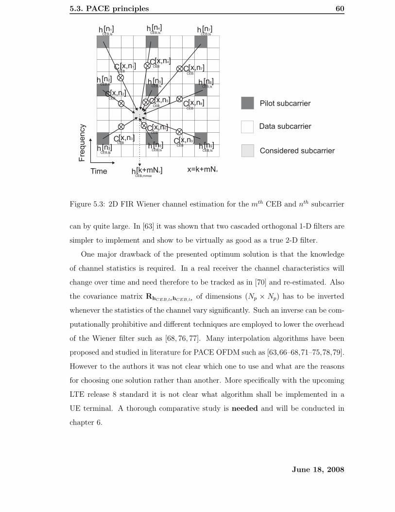
5.3. PACE principles 60
Time
Fre
quency
hCEB,mmse
[k+mN ]u
hCEB,ls
[n ]1
CCEB
[x,n ]1
C[x,n ]2
C[x,n ]3
C[x,n ]4
C[x,n ]5
C[x,n ]6
C[x,n ]7
C[x,n ]8
C[x,n ]9
Pilot subcarrier
Data subcarrier
Considered subcarrier
hCEB,ls
[n ]2
hCEB,ls
[n ]3
hCEB,ls
[n ]4
hCEB,ls
[n ]5
hCEB,ls
[n ]6
hCEB,ls
[n ]7
hCEB,ls
[n ]8
hCEB,ls
[n ]9
x=k+mNu
CEB
CEB
CEB
CEB
CEB
CEB
CEB
CEB
Figure 5.3: 2D FIR Wiener channel estimation for the mth CEB and nth subcarrier
can by quite large. In [63] it was shown that two cascaded orthogonal 1-D filters are
simpler to implement and show to be virtually as good as a true 2-D filter.
One major drawback of the presented optimum solution is that the knowledge
of channel statistics is required. In a real receiver the channel characteristics will
change over time and need therefore to be tracked as in [70] and re-estimated. Also
the covariance matrix RhCEB,lshCEB,lsof dimensions (Np × Np) has to be inverted
whenever the statistics of the channel vary significantly. Such an inverse can be com-
putationally prohibitive and different techniques are employed to lower the overhead
of the Wiener filter such as [68, 76, 77]. Many interpolation algorithms have been
proposed and studied in literature for PACE OFDM such as [63,66–68,71–75,78,79].
However to the authors it was not clear which one to use and what are the reasons
for choosing one solution rather than another. More specifically with the upcoming
LTE release 8 standard it is not clear what algorithm shall be implemented in a
UE terminal. A thorough comparative study is needed and will be conducted in
chapter 6.
June 18, 2008
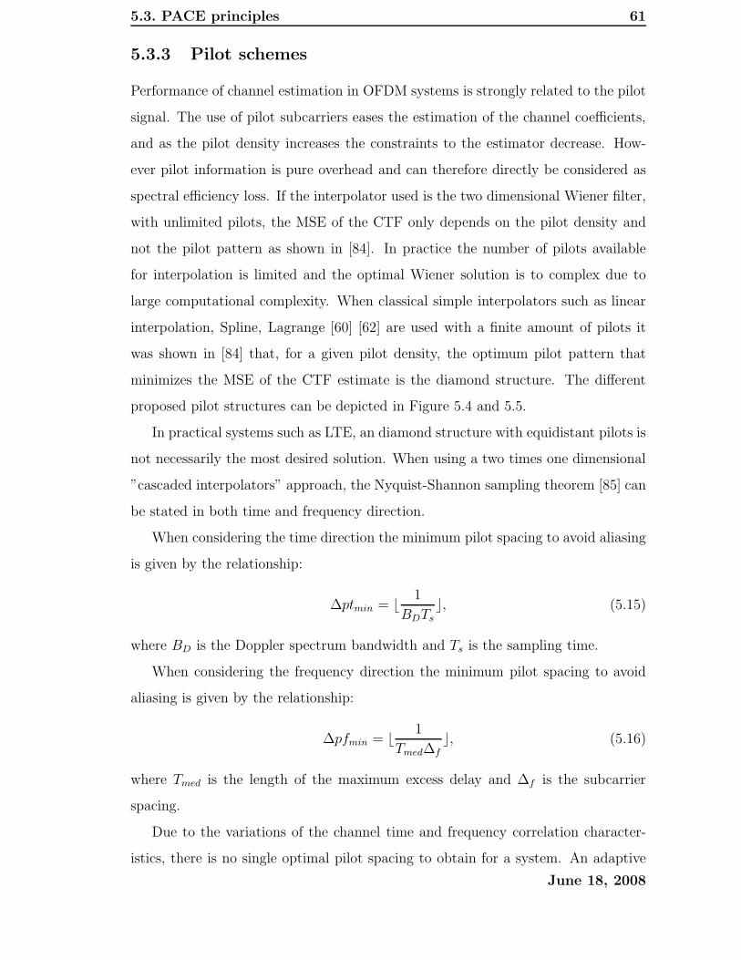
5.3. PACE principles 61
5.3.3 Pilot schemes
Performance of channel estimation in OFDM systems is strongly related to the pilot
signal. The use of pilot subcarriers eases the estimation of the channel coefficients,
and as the pilot density increases the constraints to the estimator decrease. How-
ever pilot information is pure overhead and can therefore directly be considered as
spectral efficiency loss. If the interpolator used is the two dimensional Wiener filter,
with unlimited pilots, the MSE of the CTF only depends on the pilot density and
not the pilot pattern as shown in [84]. In practice the number of pilots available
for interpolation is limited and the optimal Wiener solution is to complex due to
large computational complexity. When classical simple interpolators such as linear
interpolation, Spline, Lagrange [60] [62] are used with a finite amount of pilots it
was shown in [84] that, for a given pilot density, the optimum pilot pattern that
minimizes the MSE of the CTF estimate is the diamond structure. The different
proposed pilot structures can be depicted in Figure 5.4 and 5.5.
In practical systems such as LTE, an diamond structure with equidistant pilots is
not necessarily the most desired solution. When using a two times one dimensional
”cascaded interpolators” approach, the Nyquist-Shannon sampling theorem [85] can
be stated in both time and frequency direction.
When considering the time direction the minimum pilot spacing to avoid aliasing
is given by the relationship:
∆ptmin = ⌊1
BDTs
⌋, (5.15)
where BD is the Doppler spectrum bandwidth and Ts is the sampling time.
When considering the frequency direction the minimum pilot spacing to avoid
aliasing is given by the relationship:
∆pfmin = ⌊1
Tmed∆f
⌋, (5.16)
where Tmed is the length of the maximum excess delay and ∆f is the subcarrier
spacing.
Due to the variations of the channel time and frequency correlation character-
istics, there is no single optimal pilot spacing to obtain for a system. An adaptive
June 18, 2008
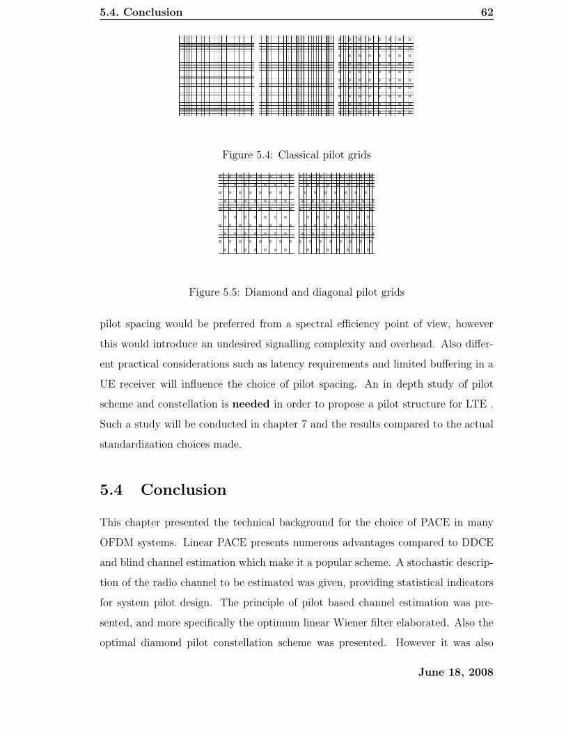
5.4. Conclusion 62
Figure 5.4: Classical pilot grids
Figure 5.5: Diamond and diagonal pilot grids
pilot spacing would be preferred from a spectral efficiency point of view, however
this would introduce an undesired signalling complexity and overhead. Also differ-
ent practical considerations such as latency requirements and limited buffering in a
UE receiver will influence the choice of pilot spacing. An in depth study of pilot
scheme and constellation is needed in order to propose a pilot structure for LTE .
Such a study will be conducted in chapter 7 and the results compared to the actual
standardization choices made.
5.4 Conclusion
This chapter presented the technical background for the choice of PACE in many
OFDM systems. Linear PACE presents numerous advantages compared to DDCE
and blind channel estimation which make it a popular scheme. A stochastic descrip-
tion of the radio channel to be estimated was given, providing statistical indicators
for system pilot design. The principle of pilot based channel estimation was pre-
sented, and more specifically the optimum linear Wiener filter elaborated. Also the
optimal diamond pilot constellation scheme was presented. However it was also
June 18, 2008

5.4. Conclusion 63
shown that for a practical system such as LTE many considerations such as system
signalling complexity, computational complexity and latency requirements had to
be taken into account. This leads to a need for thorough algorithm investigation as
well as pilot constellation and spacing studies which have respectively been carried
out in chapter 6 and chapter 7.
June 18, 2008

Chapter 6
Frequency direction interpolation
In the 3GPPP LTE specifications [4] [5] no channel interpolation algorithms are
dictated or recommended, leaving this issue open to the UE manufacturers. So
far different studies have been done for other PACE OFDM based standards such
as for the 802.11 or 802.16 families. Even though the algorithms studied in this
chapter aren’t directly novel, their behavior has not been studied previously in a
LTE context.
In this chapter, ”state-of-the-art” solutions for frequency direction PACE are
evaluated by first performing a survey of Linear algorithms. The studied solutions
are then reformulated in a discrete generic matrix-vector notation and classified ac-
cording to their a priori assumptions on channel statistics. An analytical study is
conducted leading to a generalized closed formulation. Performance is evaluated
through Monte Carlo simulations. Finally, a complexity study evaluates the com-
putational needs of the studied solutions.
6.1 Introduction
As stated in chapter 5 Hoeher showed in [63] that the two-dimensional interpolation
problem of PACE could be solved by using two cascaded orthogonal one-dimensional
filters, giving virtually no performance loss compared to the two-dimensional filter.
The latency requirements of standards such as LTE or IEEE 802.16e limit the pilot
span available for channel estimation in the time direction to a low number of
64
6.1. Introduction 65
samples. This increases the importance of the frequency-direction interpolation,
which is the focus of this chapter.
Much attention has been given to this topic showing that the performance trade-
off of the algorithms depends on the relationship between the Power Delay Profile
(PDP) properties and the frequency-domain pilot spacing. Deterministic approaches
have, so far, been separated into time- and frequency-domain solutions. Determin-
istic time-domain solutions are: the Time-Domain Least Squares (TDLS) [66, 71],
the Maximum Likelihood (ML) approach [72, 79] and the Noise Reduction Algo-
rithm (NRA) [73]. Deterministic frequency-domain methods are Spline, Gaussian
or Lagrange interpolation, and require higher pilot overhead to achieve an accept-
able performance [74]. Bayesian approaches such as the Minimum Mean Squared
Error (MMSE) estimator in time domain and/or frequency domain have been pro-
posed in [63,66], with complexity reduction by Singular Value Decomposition (SVD)
suggested in [68].
Different comparisons of these algorithms have been done. Van de Beek studies
the TDLS versus the MMSE approach in a non-sample-spaced (NSS) channel [66],
however he assumes a full bandwidth system with pilots in all subcarriers, thereby
avoiding the leakage effect on the TDLS algorithm. Edfors compares a low rank
reduction of the MMSE with a Discrete Fourier Transform (DFT) based imple-
mentation versus an SVD based [68] showing the superiority of the SVD for NSS
channels. However the MMSE can be implemented with a low complex non-DFT
based matrix, avoiding leakage, as shown by Yang [75]. Morelli compares the ML
with the MMSE approach [79] using virtual subcarriers but uses a sample-spaced
(SS) channel which favors the ML performance as no leakage is present.
In general, parameters such as the FFT size, number of virtual subcarriers, pilot
spacing, PDP and whether the channel is sample-spaced or not, have a critical
impact on formulation, performance and complexity of the studied algorithms. A
clear overview is therefore difficult to achieve from literature, and a comprehensive
comparison is needed.
The major contribution of this chapter is to provide a framework for
the choice of a channel estimation algorithm for the upcoming PACE
June 18, 2008
6.2. Classification of Channels estimation Algorithms 66
OFDM-based standards. In this study we derive a uniform algorithm and Mean
Squared Error (MSE) formulation, covering all studied algorithms and thereby fa-
cilitating a generic performance comparison. Three main effects will be studied: the
impact of a priori knowledge in a full bandwidth system with a SS channel, the effect
of virtual subcarriers and the effect of a NSS channel. Performance simulations are
conducted in a LTE context. The importance of using an interpolation algorithm
insensitive to the channel statistics at the receiver such as the Robust Wiener filter
(RW) [78] is essential to avoid the leakage effect due to NSS channel used with DFT
based solutions. However it will be demonstrated that knowledge of the exact CIR
tap delay locations is a key parameter for low MSE results.
6.2 Classification of Channels estimation Algorithms
Why doing a classification of algorithms? What is the goal and the usefulness
of such? The idea is to have a framework for a fair comparison of state of the
art solutions. This would then help to choose a channel estimation algorithm in a
system like LTE. On top of this, when new algorithms are developed, their evaluation
is eased as well as comparison with the state of art solutions. A comparison by
inspection would be sufficient to highlight the differences with the most similar
solution and thereby give an intuitive performance difference.
So far, Hanzo et. al. has made a classification of various 2D-FIR Wiener related
channel estimation approaches in [26]. These approaches use standard techniques
known from literature of multidimensional signal processing. This classification
describes complexity reduction techniques of the optimal 2D-FIR Wiener approach,
where the most relevant are:
- Hoeher proposed to select a subset of nearest pilot channel estimates based on
a derived metric [63, 64].
- Hoeher showed that ”2 times 1D” interpolation should be used instead of ”pure
2D” interpolation [63, 64].
- Edfors derived a low rank approximation technique with the aid of a Singular
June 18, 2008
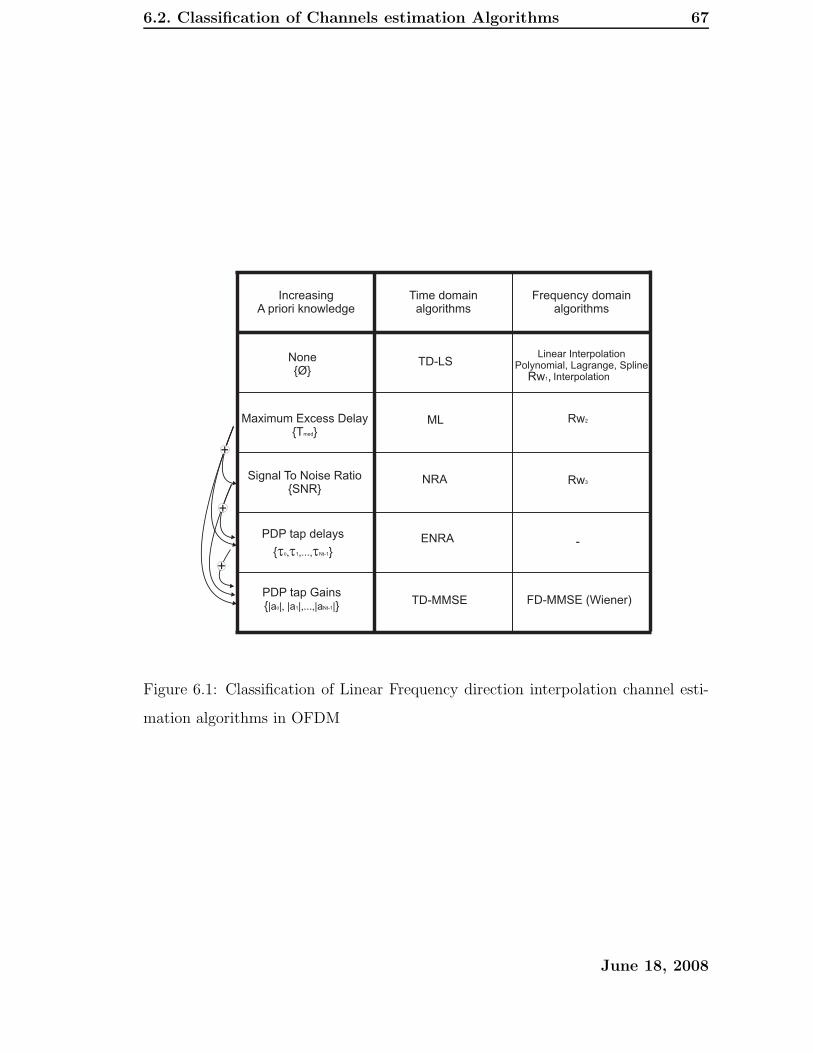
6.2. Classification of Channels estimation Algorithms 67
IncreasingA priori knowledge
Time domainalgorithms
Frequency domainalgorithms
None{Ø}
Maximum Excess Delay{T }med
Signal To Noise Ratio{SNR}
PDP tap delays
{ }...t t t0, , ,1 Nt-1
PDP tap Gains{ }|a | |a | ... |a |0 , , ,1 Nt-1
ML
TD-LS
NRA
ENRA
TD-MMSE
Linear InterpolationPolynomial, Lagrange, Spline
InterpolationRw1,
Rw3
FD-MMSE (Wiener)
+
+
+
Rw2
-
Figure 6.1: Classification of Linear Frequency direction interpolation channel esti-
mation algorithms in OFDM
June 18, 2008

6.3. Estimation Algorithms 68
Value Decomposition [68].
- Van de Beek et. al. proposed the use of a DFT instead of the unitary linear
transform employed int the SVD-based filter [66].
More recently Tolochko focused his work on MMSE based algorithms with an
emphasis on statistical parameter estimation in [69].
Despite the previous work, an in depth comparison, including time domain and
frequency domain approaches, is not known to the author. Different limited com-
parisons have been made in several publications, such as in [66, 68, 75, 79], but in
section 6.1, none of these comparisons give a clear overview over the existing linear
solutions. Other non-MMSE based techniques should therefore also be considered.
A broader classification is then needed, and will be carried out in the following. A
priori knowledge together with a separation into time domain and frequency domain
approaches will determine the ”type” of algorithm considered. Figure 6.1 illustrates
how the algorithms can be classified into time and frequency domain approaches,
also the dependency of the studied algorithms on a priori information is brought to
evidence.
6.3 Estimation Algorithms
All the different channel estimators are based on an initial Least Squares (LS) esti-
mate of the channel response at pilot positions hls ∈ CNp, which is obtained as:
hls = Dp−1yp = hp + Dp
−1wp (6.1)
It is assumed that the pilot symbols are M-PSK modulated with unit power, so
that the noise in the LS estimate Dp−1wp has the same statistical properties as
wp. Furthermore, the number of pilot symbols Np, is assumed to be larger than the
normalized maximum excess delay of the channel,τNt−1
τs.
In the following, two scenarios are considered:
Case 1 A SS-CIR scenario, where it is assumed that the delays τi are sample
spaced on the same grid as the receiver and all τi
τsare integer values.
June 18, 2008
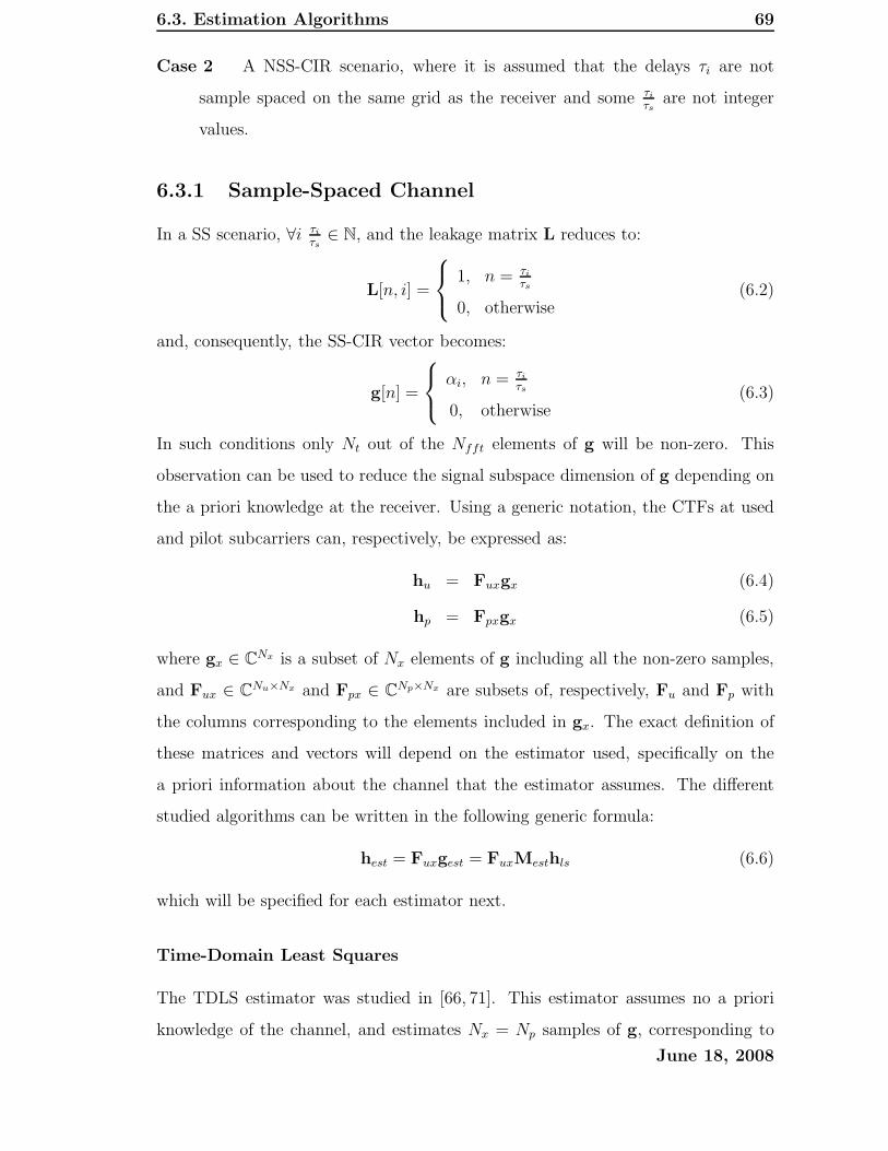
6.3. Estimation Algorithms 69
Case 2 A NSS-CIR scenario, where it is assumed that the delays τi are not
sample spaced on the same grid as the receiver and some τi
τsare not integer
values.
6.3.1 Sample-Spaced Channel
In a SS scenario, ∀i τi
τs∈ N, and the leakage matrix L reduces to:
L[n, i] =
1, n = τi
τs
0, otherwise(6.2)
and, consequently, the SS-CIR vector becomes:
g[n] =
αi, n = τi
τs
0, otherwise(6.3)
In such conditions only Nt out of the Nfft elements of g will be non-zero. This
observation can be used to reduce the signal subspace dimension of g depending on
the a priori knowledge at the receiver. Using a generic notation, the CTFs at used
and pilot subcarriers can, respectively, be expressed as:
hu = Fuxgx (6.4)
hp = Fpxgx (6.5)
where gx ∈ CNx is a subset of Nx elements of g including all the non-zero samples,
and Fux ∈ CNu×Nx and Fpx ∈ CNp×Nx are subsets of, respectively, Fu and Fp with
the columns corresponding to the elements included in gx. The exact definition of
these matrices and vectors will depend on the estimator used, specifically on the
a priori information about the channel that the estimator assumes. The different
studied algorithms can be written in the following generic formula:
hest = Fuxgest = FuxMesthls (6.6)
which will be specified for each estimator next.
Time-Domain Least Squares
The TDLS estimator was studied in [66, 71]. This estimator assumes no a priori
knowledge of the channel, and estimates Nx = Np samples of g, corresponding to
June 18, 2008
6.3. Estimation Algorithms 70
gp[n] = g[n] for 0 ≤ n ≤ Np − 1. The formulation of TDLS is:
htdls = Fupgtdls = FupF−1pp hls (6.7)
where Fpp ∈ CNp×Np and Fup ∈ CNu×Np correspond, respectively, to Fpp[m,n] =
Fp[m,n] and Fup[k, n] = Fu[k, n] for 0 ≤ n ≤ Np − 1. For the TDLS estimator,
then, Mest = F−1pp . Note that Fpp is always invertible due to the Vandermonde
structure of the DFT matrix [71]; however, in a Partial Bandwidth scenario, this
matrix can become ill-conditioned depending on the number of virtual subcarriers.
Maximum Likelihood
The ML estimator, proposed in [72, 79], assumes that the receiver knows the CIR
length, i.e, the last channel CIR tap’s delay τNt−1, and only estimates the Nx =
Ns =τNt−1
τs+ 1 first samples of the SS-CIR, corresponding to gs[n] = g[n] for
0 ≤ n ≤ Ns − 1. The ML estimator is expressed as:
hml = Fusgml = Fus(FHpsFps)
−1FHpshls (6.8)
where Fps ∈ CNp×Ns and Fus ∈ CNu×Ns correspond, respectively, to Fps[m,n] =
Fp[m,n] and Fus[k, n] = Fu[k, n] for 0 ≤ n ≤ Ns − 1. In this case, Mest =
(FHpsFps)
−1FHps. Similarly to the case of the TDLS estimator, the matrix Fps is
always of full column rank (for Np ≥ Ns), implying that FHpsFps is of full rank. How-
ever, in the presence of virtual subcarriers this matrix can become ill-conditioned, as
for the TDLS estimator. In appendix C.3 more details on the properties of FHpsFps
are given.
Noise Reduction Algorithm
As a solution to the ill-conditioning problems of the previous estimators, a small
value can be added to the diagonal of the matrix to be inverted [73], thus avoiding
numerical instability. This is also known as Tikhonov regularization [81], a method
to improve the conditioning of an ill-posed problem. This modification leads to the
following expression of the NRA:
hnra = Fusgnra = Fus(FHpsFps + γnraIs)
−1FHpshls (6.9)
June 18, 2008
6.3. Estimation Algorithms 71
where Is is the identity matrix of size Ns, and γnra is a positive scalar value. From
(6.9), it follows that Mest = (FHpsFps + γnraIs)
−1FHps. In a Full Bandwidth scenario
with evenly spaced pilot subcarriers, it can be shown that the optimum value is
γnra = Nsσ2w. Furthermore, the NRA with this value is equivalent to the robust
Wiener filter estimator proposed in [68, 78], as it is proven in appendix C.1. The
effect of variation of this value on MSE is given in appendix C.5.
Enhanced Noise Reduction Algorithm
The Enhanced Noise Reduction Algorithm (ENRA) differs from the NRA by only
estimating the Nx = Nt samples of g which are not null, i.e., gt[n] = g[τn/τs] for
0 ≤ n ≤ Nt − 1. Therefore, the knowledge of the number of CIR taps and their
corresponding delays is required. The estimator is given by:
henra = Futgenra = Fut(FHptFpt + γenraIt)
−1FHpthls (6.10)
where Fpt ∈ CNp×Nt and Fus ∈ CNu×Nt correspond, respectively, to Fpt[m,n] =
Fp[m, τn/τs] and Fut[k, n] = Fu[k, τn/τs] for 0 ≤ n ≤ Nt − 1. It denotes the identity
matrix of size Nt. Hence, for the ENRA Mest = (FHptFpt+γenraIt)
−1FHpt. Analogously
to the NRA, the value γenra = Ntσ2w is optimum in a Full Bandwidth with equally
spaced pilots scenario, and will be assumed in the following. It can be observed that
this estimator corresponds to the one proposed in [75], when the CIR tap gains’
average powers are not known and the CIR tap delays are sample-spaced.
Wiener Filter
The Wiener filter (WF) estimator minimizes the MSE of the estimate by making
use of channel and noise correlation properties, and has been broadly treated in
literature [63, 68, 75, 78]. It is classically formulated as:
hwf = Rhuhp(Rhphp
+ σ2wIp)
−1hls (6.11)
where Rhuhp= E{huh
Hp } is the correlation matrix of hu and hp, Rhphp
= E{hphHp }
is the autocorrelation matrix of hp, and Ip is the identity matrix of size Np. In the
sample spaced case, these frequency correlation matrices become:
Rhuhp= FutRgtgt
FHpt (6.12)
June 18, 2008

6.3. Estimation Algorithms 72
Rhphp= FptRgtgt
FHpt (6.13)
where Rgtgt= E{gtg
Ht } is the autocorrelation matrix of gt. Inserting (6.12) and
(6.13) in (6.11), and using the matrix relation ABH(I + BABH)−1 = (A−1 +
BHB)−1BH [25], leads to:
hwf = Futgwf = Fut(FHptFpt + σ2
wR−1gtgt
)−1FHpthls (6.14)
which is equivalent to the estimator proposed by Yang in [75] when considering
sample spaced channels. For WF, Mest = (FHptFpt + σ2
wR−1gtgt
)−1FHpt.
Note that when no information about the channel correlation is available, a
robust sample-spaced design of the wiener filter is shown in [44]. To obtain this
sample-spaced robust estimate hssrw it is assumed that the PDP is sample-spaced
with Ns samples of equal mean power in all taps. In such conditions Fut = Fus,
Fpt = Fps and Rgtgt= 1
NsIs. In [44] the authors proved that this robust WF estimate
hssrw is fully equivalent to the NRA estimate hnra given in (6.9). The mathematical
derivations are given in appendix C.1.
Generic Formulation
When observing the expressions of the studied algorithms, a general formulation
that covers all the cases can be given by:
hest = Fuxgest = Fux(FHpxFpx + γestCest)
−1FHpxhls (6.15)
An overview over the specific values taken by each element of (6.15) is given in Table
6.1.
MSE of the Estimators
The different studied estimators are all described by (6.6). It is then possible to
evaluate their respective performance by using one single generic MSE expression.
The MSE is calculated as:
MSE{hest[k]} = E{|hu[k] − hest[k]|2} (6.16)
Using (6.6), the MSE for the kth subcarrier becomes:
MSE{hest[k]} = Q[k, k] (6.17)
June 18, 2008
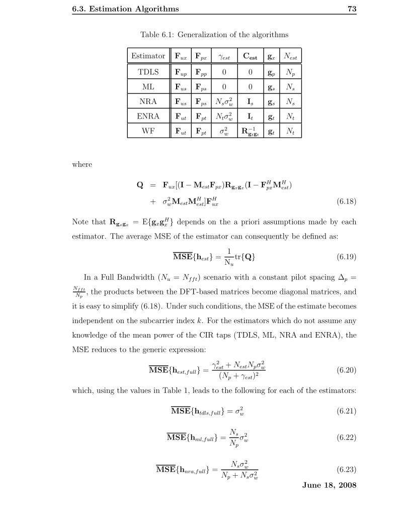
6.3. Estimation Algorithms 73
Table 6.1: Generalization of the algorithms
Estimator Fux Fpx γest Cest gx Nest
TDLS Fup Fpp 0 0 gp Np
ML Fus Fps 0 0 gs Ns
NRA Fus Fps Nsσ2w Is gs Ns
ENRA Fut Fpt Ntσ2w It gt Nt
WF Fut Fpt σ2w R−1
gtgtgt Nt
where
Q = Fux[(I − MestFpx)Rgxgx(I − FH
pxMHest)
+ σ2wMestM
Hest]F
Hux (6.18)
Note that Rgxgx= E{gxg
Hx } depends on the a priori assumptions made by each
estimator. The average MSE of the estimator can consequently be defined as:
MSE{hest} =1
Nu
tr{Q} (6.19)
In a Full Bandwidth (Nu = Nfft) scenario with a constant pilot spacing ∆p =
Nfft
Np, the products between the DFT-based matrices become diagonal matrices, and
it is easy to simplify (6.18). Under such conditions, the MSE of the estimate becomes
independent on the subcarrier index k. For the estimators which do not assume any
knowledge of the mean power of the CIR taps (TDLS, ML, NRA and ENRA), the
MSE reduces to the generic expression:
MSE{hest,full} =γ2
est +NestNpσ2w
(Np + γest)2(6.20)
which, using the values in Table 1, leads to the following for each of the estimators:
MSE{htdls,full} = σ2w (6.21)
MSE{hml,full} =Ns
Np
σ2w (6.22)
MSE{hnra,full} =Nsσ
2w
Np +Nsσ2w
(6.23)
June 18, 2008
6.3. Estimation Algorithms 74
MSE{henra,full} =Ntσ
2w
Np +Ntσ2w
(6.24)
When the mean powers of each CIR tap are known, we have for the WF estimator:
MSE{hwf,full} =∑Nt−1
i=0
{
Rgtgt[i]
(
1 −NpRgtgt [i]
σ2w+NpRgtgt [i]
)2
+σ2wNp
(
Rgtgt [i]
σ2w+NpRgtgt [i]
)2}
(6.25)
Observations
Different observations can be done for each algorithm:
i) For the TDLS estimator, no a priori channel knowledge is needed. The matrix
to be inverted, Fpp, is static, can be precalculated and stored in memory.
If the matrix is ill-conditioned, the algorithm is not usable, otherwise the
performance depends only on σ2w.
ii) For the ML estimator, knowledge of the CIR length Ns is needed. The matrix
FHpsFps is always of full rank, and can also be precalculated and stored in mem-
ory for different CIR lengths. When ill-conditioned it is also not applicable.
It outperforms the TDLS estimator unless:
{Ns = Np} ⇒ {hml = htdls}.
iii) For the NRA, knowledge of the CIR length Ns and σ2w is needed. In the
same way as for the ML approach, matrices can be precalculated and stored
in memory. The ill-conditioning effect disappears and the NRA outperforms
the ML estimator. As the SNR increases it follows that:
{σ2w → 0} ⇒ {hnra → hml}
({σ2w → 0} ∧ {Ns = Np}) ⇒ {hnra → htdls}.
iv) For the ENRA, exact tap delay and σ2w knowledge is required. The matrix
of size (Nt × Nt) to be inverted is dynamic and must therefore be computed
each time a tap delay changes. The ENRA outperforms the NRA if Nt < Ns,
otherwise:
{Nt = Ns} ⇒ {henra = hnra}.
June 18, 2008
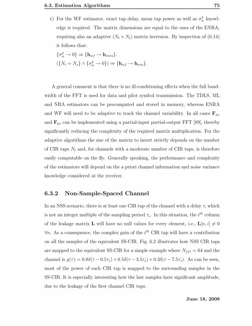
6.3. Estimation Algorithms 75
v) For the WF estimator, exact tap delay, mean tap power as well as σ2w knowl-
edge is required. The matrix dimensions are equal to the ones of the ENRA,
requiring also an adaptive (Nt ×Nt) matrix inversion. By inspection of (6.14)
it follows that:
{σ2w → 0} ⇒ {hwf → henra}.
({Nt = Ns} ∧ {σ2w → 0}) ⇒ {hwf → hnra}.
A general comment is that there is no ill-conditioning effects when the full band-
width of the FFT is used for data and pilot symbol transmission. The TDLS, ML
and NRA estimators can be precomputed and stored in memory, whereas ENRA
and WF will need to be adaptive to track the channel variability. In all cases Fux
and Fpx can be implemented using a partial-input partial-output FFT [89], thereby
significantly reducing the complexity of the required matrix multiplication. For the
adaptive algorithms the size of the matrix to invert strictly depends on the number
of CIR taps Nt and, for channels with a moderate number of CIR taps, is therefore
easily computable on the fly. Generally speaking, the performance and complexity
of the estimators will depend on the a priori channel information and noise variance
knowledge considered at the receiver.
6.3.2 Non-Sample-Spaced Channel
In an NSS scenario, there is at least one CIR tap of the channel with a delay τi which
is not an integer multiple of the sampling period τs. In this situation, the ith column
of the leakage matrix L will have no null values for every element, i.e., L[n, i] 6= 0
∀n. As a consequence, the complex gain of the ith CIR tap will have a contribution
on all the samples of the equivalent SS-CIR. Fig. 6.2 illustrates how NSS CIR taps
are mapped to the equivalent SS-CIR for a simple example where Nfft = 64 and the
channel is g(τ) = 0.8δ(τ − 0.5τs)+ 0.5δ(τ − 3.5τs)+ 0.3δ(τ − 7.5τs). As can be seen,
most of the power of each CIR tap is mapped to the surrounding samples in the
SS-CIR. It is especially interesting how the last samples have significant amplitude,
due to the leakage of the first channel CIR taps.
June 18, 2008
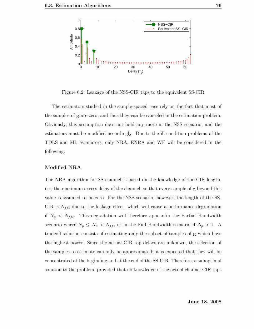
6.3. Estimation Algorithms 76
0 10 20 30 40 50 600
0.2
0.4
0.6
0.8
1
Delay (τs)
Am
plitu
de
NSS−CIREquivalent SS−CIR
Figure 6.2: Leakage of the NSS-CIR taps to the equivalent SS-CIR
The estimators studied in the sample-spaced case rely on the fact that most of
the samples of g are zero, and thus they can be canceled in the estimation problem.
Obviously, this assumption does not hold any more in the NSS scenario, and the
estimators must be modified accordingly. Due to the ill-condition problems of the
TDLS and ML estimators, only NRA, ENRA and WF will be considered in the
following.
Modified NRA
The NRA algorithm for SS channel is based on the knowledge of the CIR length,
i.e., the maximum excess delay of the channel, so that every sample of g beyond this
value is assumed to be zero. For the NSS scenario, however, the length of the SS-
CIR is Nfft due to the leakage effect, which will cause a performance degradation
if Np < Nfft. This degradation will therefore appear in the Partial Bandwidth
scenario where Np ≤ Nu < Nfft or in the Full Bandwidth scenario if ∆p > 1. A
tradeoff solution consists of estimating only the subset of samples of g which have
the highest power. Since the actual CIR tap delays are unknown, the selection of
the samples to estimate can only be approximated: it is expected that they will be
concentrated at the beginning and at the end of the SS-CIR. Therefore, a suboptimal
solution to the problem, provided that no knowledge of the actual channel CIR taps
June 18, 2008

6.3. Estimation Algorithms 77
is available, is given by the Modified NRA, (MNRA), which is formulated as:
hmnra = Fumgmnra
= Fum(FHpmFpm + γmnraIm)−1FH
pmhls
(6.26)
where the matrix Fum ∈ CNu×Nm is defined as:
Fum[k, n] =
Fu[k, n], 0 ≤ n ≤ ⌈Nm(1 − α)⌉ − 1
Fu[k,Nfft −Nm + n], ⌈Nm(1 − α)⌉ ≤ n ≤ Nm − 1
(6.27)
and Fpm ∈ CNp×Nu is defined analogously with respect to Fp. Im is the identity
matrix of size Nm. Furthermore, the parameter γmnra is selected to be γmnra =
Nmσ2w, analogously to the sample-spaced case.
Two parameters shall be adapted depending on the PDP and σ2w: Nm represent-
ing the number of samples of the equivalent SS-CIR to estimate, and α representing
the proportion of the estimated samples in the final part of the SS-CIR.
ENRA and Wiener Filter
When using the ENRA or the Wiener Filter estimator, it is assumed that the delays
of the channel are perfectly known, so that there is no need to estimate the equivalent
SS-CIR. Instead, the parameters to estimate are the complex gains ai of each of the
CIR taps, represented by the vector a. The estimators can be rewritten for the NSS
scenario as:
henra = Tuaenra = Tu(THp Tp + γenraIt)
−1THp hls (6.28)
hwf = Tuawf = Tu(THp Tp + σ2
wR−1aa )TH
p hls (6.29)
where the matrices Tu ∈ CNu×Nt and Tp ∈ C
Np×Nt are defined with respect to
T in the same way as Fu and Fp with respect to F. As in the SS case, γenra =
σ2wNt, and Raa ∈ CNt×Nt is the correlation matrix of the channel gains, i.e, Raa =
diag{E{|a0|2}, . . . ,E{|aNt−1|
2}} as we assume i.i.d. channel taps.
The formulation in 6.29 requires exact knowledge of the delay locations. When
no statistical knowledge is available from the channel this formulation is no longer
possible. It then comes naturally to use the known formulation of 6.11 and define the
June 18, 2008

6.4. Performance evaluation 78
correlation matrices according to the assumption of Non-sample-spaced PDP with
uniformly and independently distributed tap delays τi over [0, Tmed]. According to
the derivations in appendix C.4 the CTF correlation matrix can then be given by:
Rhh[k, k′] =1 − e
−j2π(k−k′)Nfft
Tmed
j2π (k−k′)Nfft
Tmed
, (6.30)
where, RhuhpRhphp
are subsets of Rhh. hu and hp are respectively defined in
equations 2.47 and 2.49. When no information is available on the CIR MED, and
Tmed is replaced by the duration of the CP length Tg we denote this estimate by
RW1. When the CIR MED is known to the receiver we denote the estimate by RW2
and finally when the SNR is also known we denote the estimate by RW3.
MSE of the Estimators
Unlike the SS scenario, it is difficult to find a general expression that includes all
the studied algorithms for an NSS channel. For this reason, we will study the
performance of a generic estimator such as:
hest = Mesthls (6.31)
which includes any linear estimator that can be expressed in matrix form. With this
formulation, the MSE over an NSS channel is:
MSE{hest} = 1Nu
tr
{
TuRaaTHu
−TuRaaTHp MH
est − MestTpRaaTHu
+MestTpRaaTHp MH
est + σ2wMestM
Hest
}
(6.32)
and the specific values of Mest for each studied algorithm are:
Mest =
Fum(FHpmFpm + γmnraIm)−1FH
pm, MNRA
Tu(THp Tp + γenraIt)
−1THp , ENRA
Tu(THp Tp + σ2
wR−1aa )TH
p , WF
(6.33)
6.4 Performance evaluation
In the following, the performance of the estimators discussed in section 6.3 will be
studied via Monte Carlo simulations. A single-input single-output OFDM system
June 18, 2008

6.4. Performance evaluation 79
with physical layer parameters proposed for the downlink of UTRA LTE will be
used [1]. These parameters are given in Table 6.2. QPSK modulation is used for
both pilot and data symbols. Evenly spaced pilot symbols with a spacing of ∆p = 6
subcarriers are transmitted in every OFDM block.
Table 6.2: Simulation parameters
Parameter Value
Sampling frequency 30.72 MHz
τs 32.552 ns
CP length 4.69 µs
Pilot spacing 6
Nfft 2048
Subcarrier spacing 15 KHz
In Table A.3 of appendix A, three channel power delay profiles with 20 taps are
given for this simulation study. The “long SS” profile is sample spaced of length
3.711 µs, the “long NSS” profile is not sample spaced differing by 0.5 Ts from the
“long SS” profile and the “short NSS” is also not sample spaced with a length of
only 0.635 µs. Results for both MSE and uncoded Bit Error Rate (BER) using the
studied estimators as a function of the Signal-to-Noise Ratio (SNR) will be given.
The SNR will be expressed as signal-to-noise ratio per bit ( Eb
N0) [31], which in the
case of QPSK modulation corresponds to:
Eb
N0
(dB) = 10 log10
(
1
2σ2w
)
(6.34)
since the symbols are assumed to have unit power.
6.4.1 Full Bandwidth and Sample-Spaced Scenario
The performance of the different studied algorithms in a Full Bandwidth system
using the “long SS” channel profile is depicted in Fig. 6.3. As can be seen in
Fig. 6.3(a), the MSE results obtained by simulation correspond to the theoretical
June 18, 2008

6.4. Performance evaluation 80
values given in section 6.3.1. TDLS has the largest MSE among the estimators. The
ML estimator performs equal to the NRA at sufficiently high SNR, and the same
effect can be seen with ENRA and WF. As a general result, the MSE’s of NRA
and ML will always be between the ones obtained with TDLS and ENRA: for short
CIRs, the MSE will approach the one of the ENRA, and it will be closer to the
TDLS for long CIRs. From the BER results shown in 6.3(b), we see that the TDLS
curve lies 3.5 dB from the known channel performance at Eb
N0=10 dB, whereas this
distance is reduced to 0.25 dB for the ENRA and WF estimators.
6.4.2 Partial Bandwidth and Sample-Spaced Scenario
The effect of introducing virtual subcarriers at the band edges will be studied in the
following. The simulations done for the full bandwidth scenario have been repeated
with the difference that Nu=1200, as suggested in the LTE standard [1]. MSE and
BER results are given in Fig. 6.4. It is noted that in this specific case the ill-
conditioning of Fpp and (FHpsFps) will lead to a BER of 0.5 for TDLS and ML, and
a very high MSE which is out of the range of Fig. 6.4(a). The performance of NRA,
ENRA and WF is slightly deteriorated compared to Full Bandwidth as the total
number of pilot subcarriers decreases due to the constant pilot spacing.
In Fig. 6.5, the MSE of the ML estimator is analyzed as a function of the as-
sumed maximum delay of the channel (Ns) using (6.19), where different number
of used subcarriers have been represented at Eb
N0=15 dB. When all the subcarriers
are used (Nu = 2048), the error of the estimate grows linearly with the assumed
channel length. When virtual subcarriers are introduced, however, the matrix to be
inverted, FHpsFps, becomes ill-conditioned after a certain channel length, yielding a
large degradation of the MSE that makes the estimator unusable. The maximum
channel excess delay before the estimator becomes unstable decreases as the number
of used subcarriers is reduced. Note that the same effect can be seen for the TDLS
estimator, which is equivalent to the ML when the assumed CIR length is set to
(Np − 1)τs.
June 18, 2008

6.4. Performance evaluation 81
−10 −5 0 5 10 15 20 25−40
−35
−30
−25
−20
−15
−10
−5
0
5
Eb/No (dB)
MS
E (
dB)
TDLSMLNRAENRAWiener
(a)
−10 −5 0 5 10 15 20 2510
−3
10−2
10−1
Eb/No (dB)
BE
R
TDLSMLNRAENRAWienerKnown Channel
(b)
Figure 6.3: Performance of the different estimators in a Full Bandwidth OFDM
system (Nu = Nfft = 2048) and a pilot spacing of 6 for the “long” SS channel. (a)
MSE. (b) BER.
June 18, 2008

6.4. Performance evaluation 82
−10 −5 0 5 10 15 20 25−40
−35
−30
−25
−20
−15
−10
−5
0
5
Eb/No (dB)
MS
E (
dB)
NRAENRAWiener
(a)
−10 −5 0 5 10 15 20 2510
−3
10−2
10−1
Eb/No (dB)
BE
R
TDLSMLNRAENRAWienerKnown Channel
(b)
Figure 6.4: Performance of the different estimators in an LTE scenario with Nu =
1200, Nfft = 2048 and a pilot spacing of 6 for the “long” SS channel. (a) MSE. (b)
BER.
June 18, 2008

6.4. Performance evaluation 83
0 0.5 1 1.5 2 2.5 3 3.5 4−40
−35
−30
−25
−20
−15
−10
Length of uniform CIR (µs)
MS
E (
dB)
Nu = 400
Nu = 800
Nu = 1200
Nu = 1600
Nu = 2048
Figure 6.5: MSE of the ML estimator for varying assumed CIR length and different
Nu, Nfft = 2048 and Eb/No = 15 dB
6.4.3 Non-Sample-Spaced Scenario
In a first step, the effect of having an NSS PDP on the classical algorithms will
be studied. The MSE and BER results are given in Fig. 6.6 for the NRA, RW,
ENRA and WF in the exact same scenario as for Fig. 6.4, but using the “long NSS”
channel profile. It is noted that the ENRA and WF have the same performance
as when employing the “long SS” PDP. The NRA, on the other hand, suffers from
significant degradation for Eb
N0≥10 dB in both MSE and BER. The RW used is
RW3 for simplicity. From these results it can be observed that the RW, ENRA and
WF are not affected by the leakage effect. The knowledge of the tap delays of the
PDP gives an advantage of the ENRA and WF over the RW of approx. 1dB in the
studied scenario for the BER plot. It is noted that varying the PDP will influence
this gain.
In Fig. 6.7 the robustness of the ENRA against delay estimation errors is studied.
A random zero-mean Gaussian error with variance σ2τ has been added to the delay’s
values to simulate imperfect delay estimates, and the MSE of the estimates has
June 18, 2008

6.4. Performance evaluation 84
−10 −5 0 5 10 15 20 25−40
−35
−30
−25
−20
−15
−10
−5
0
5
Eb/No (dB)
MS
E (
dB)
NRAENRAWienerRW (NSS)
(a)
−10 −5 0 5 10 15 20 2510
−3
10−2
10−1
Eb/No (dB)
BE
R
NRAENRAWienerKnown ChannelRW (NSS)
(b)
Figure 6.6: Effect of leakage on the classical algorithms in an LTE scenario with
Nu = 1200, Nfft = 2048 and a pilot spacing of 6 for the “long” NSS channel. (a)
MSE. (b) BER.
June 18, 2008

6.4. Performance evaluation 85
−10 −5 0 5 10 15 20 25−40
−35
−30
−25
−20
−15
−10
−5
0
5
Eb/No (dB)
MS
E (
dB)
σt2=0.01
σt2=0.001
σt2=0.0001
σt2=0
Figure 6.7: MSE of the ENRA with different delay estimation errors in an LTE
scenario with Nu = 1200, Nfft = 2048 and a pilot spacing of 6 for the “long” NSS
channel.
−10 −5 0 5 10 15 20 250
20
40
60
80
100
120
140
160
180
200
Eb/No (dB)
Nm
NSS long α = 0.33
NSS long α = 0.50
NSS short α = 0.33
NSS short α = 0.50
Figure 6.8: Optimal Nm for MNRA in a nLTE scenario with Nu = 1200, Nfft =
2048 and a pilot spacing of 6 for the “long” and “short” NSS channels.
June 18, 2008
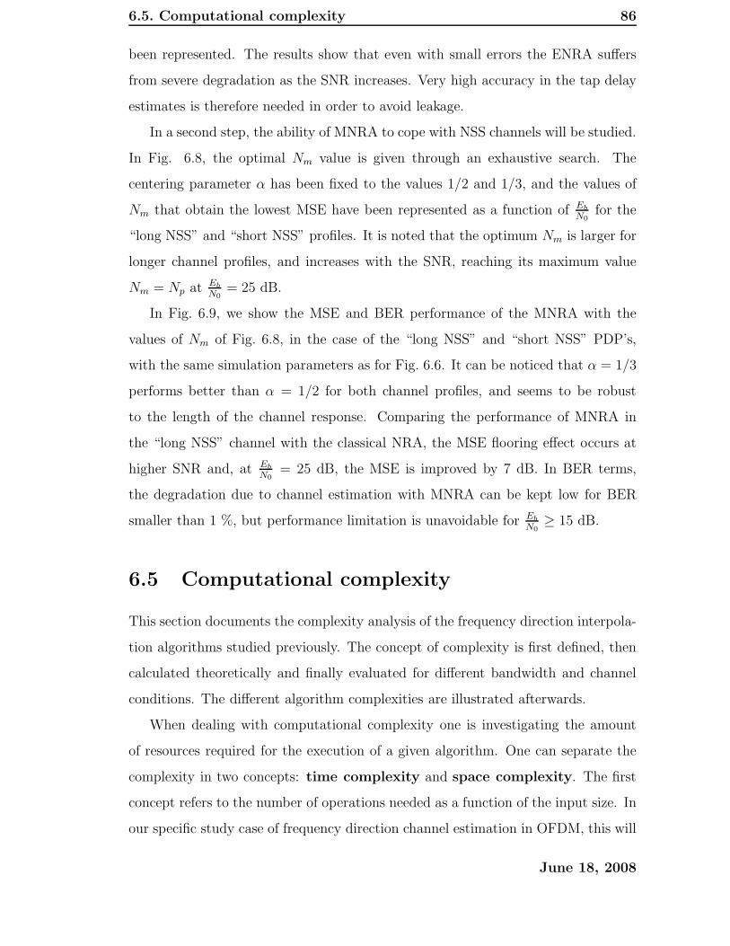
6.5. Computational complexity 86
been represented. The results show that even with small errors the ENRA suffers
from severe degradation as the SNR increases. Very high accuracy in the tap delay
estimates is therefore needed in order to avoid leakage.
In a second step, the ability of MNRA to cope with NSS channels will be studied.
In Fig. 6.8, the optimal Nm value is given through an exhaustive search. The
centering parameter α has been fixed to the values 1/2 and 1/3, and the values of
Nm that obtain the lowest MSE have been represented as a function of Eb
N0for the
“long NSS” and “short NSS” profiles. It is noted that the optimum Nm is larger for
longer channel profiles, and increases with the SNR, reaching its maximum value
Nm = Np at Eb
N0= 25 dB.
In Fig. 6.9, we show the MSE and BER performance of the MNRA with the
values of Nm of Fig. 6.8, in the case of the “long NSS” and “short NSS” PDP’s,
with the same simulation parameters as for Fig. 6.6. It can be noticed that α = 1/3
performs better than α = 1/2 for both channel profiles, and seems to be robust
to the length of the channel response. Comparing the performance of MNRA in
the “long NSS” channel with the classical NRA, the MSE flooring effect occurs at
higher SNR and, at Eb
N0= 25 dB, the MSE is improved by 7 dB. In BER terms,
the degradation due to channel estimation with MNRA can be kept low for BER
smaller than 1 %, but performance limitation is unavoidable for Eb
N0≥ 15 dB.
6.5 Computational complexity
This section documents the complexity analysis of the frequency direction interpola-
tion algorithms studied previously. The concept of complexity is first defined, then
calculated theoretically and finally evaluated for different bandwidth and channel
conditions. The different algorithm complexities are illustrated afterwards.
When dealing with computational complexity one is investigating the amount
of resources required for the execution of a given algorithm. One can separate the
complexity in two concepts: time complexity and space complexity. The first
concept refers to the number of operations needed as a function of the input size. In
our specific study case of frequency direction channel estimation in OFDM, this will
June 18, 2008
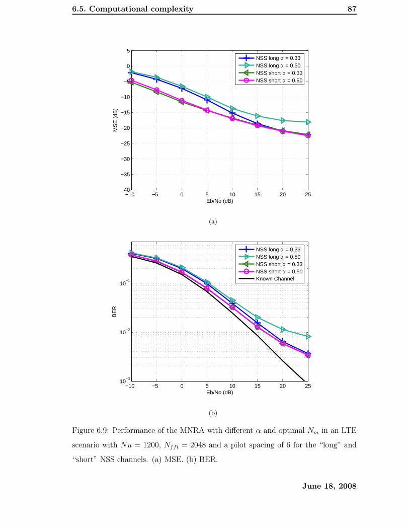
6.5. Computational complexity 87
−10 −5 0 5 10 15 20 25−40
−35
−30
−25
−20
−15
−10
−5
0
5
Eb/No (dB)
MS
E (
dB)
NSS long α = 0.33NSS long α = 0.50NSS short α = 0.33NSS short α = 0.50
(a)
−10 −5 0 5 10 15 20 2510
−3
10−2
10−1
Eb/No (dB)
BE
R
NSS long α = 0.33NSS long α = 0.50NSS short α = 0.33NSS short α = 0.50Known Channel
(b)
Figure 6.9: Performance of the MNRA with different α and optimal Nm in an LTE
scenario with Nu = 1200, Nfft = 2048 and a pilot spacing of 6 for the “long” and
“short” NSS channels. (a) MSE. (b) BER.
June 18, 2008
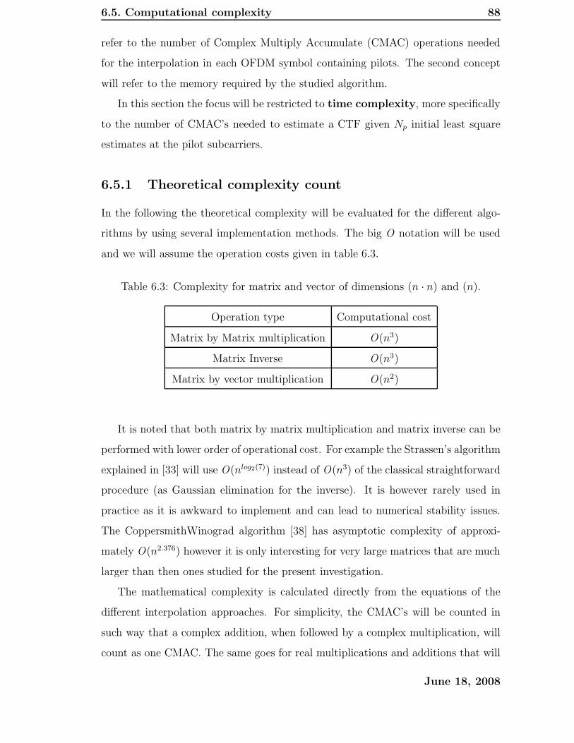
6.5. Computational complexity 88
refer to the number of Complex Multiply Accumulate (CMAC) operations needed
for the interpolation in each OFDM symbol containing pilots. The second concept
will refer to the memory required by the studied algorithm.
In this section the focus will be restricted to time complexity, more specifically
to the number of CMAC’s needed to estimate a CTF given Np initial least square
estimates at the pilot subcarriers.
6.5.1 Theoretical complexity count
In the following the theoretical complexity will be evaluated for the different algo-
rithms by using several implementation methods. The big O notation will be used
and we will assume the operation costs given in table 6.3.
Table 6.3: Complexity for matrix and vector of dimensions (n · n) and (n).
Operation type Computational cost
Matrix by Matrix multiplication O(n3)
Matrix Inverse O(n3)
Matrix by vector multiplication O(n2)
It is noted that both matrix by matrix multiplication and matrix inverse can be
performed with lower order of operational cost. For example the Strassen’s algorithm
explained in [33] will use O(nlog2(7)) instead of O(n3) of the classical straightforward
procedure (as Gaussian elimination for the inverse). It is however rarely used in
practice as it is awkward to implement and can lead to numerical stability issues.
The CoppersmithWinograd algorithm [38] has asymptotic complexity of approxi-
mately O(n2.376) however it is only interesting for very large matrices that are much
larger than then ones studied for the present investigation.
The mathematical complexity is calculated directly from the equations of the
different interpolation approaches. For simplicity, the CMAC’s will be counted in
such way that a complex addition, when followed by a complex multiplication, will
count as one CMAC. The same goes for real multiplications and additions that will
June 18, 2008

6.5. Computational complexity 89
also give a CMAC.
The different complexity orders of the different interpolation algorithms can be
appreciated in table 6.4.
Table 6.4: Complexity order of the different algorithms
Algorithm Complexity
TDLS Method 1 O(Nu ·Np)
TDLS Method 2 O(Nfft · log2(Nfft) +N2p )
TDLS Method 3 O(αu ·Nfft · log2(Nfft) +N2p )
ML/NRA Method 1 O(Nu ·Np)
ML/NRA Method 2 O(Tmed · (Nu +Np))
ML/NRA Method 3 O(αu ·Nfft · log2(Nfft) + Tmed ·Np)
ENRA/WF O(Nt · (Nu +N2t +Np))
RWF O(Nu ·Np)
SVD O(Ne · (Nu +Ne +Np))
It is noted that the complexity calculation assumes that the a priori information
on CIR length, SNR, CIR tap delays and powers are given to the receiver and not
estimated. Therefore complexity overhead due to statistics estimation has not been
included in this study.
TDLS: Method 1 is the straightforward direct matrix implementation with Np
multiplications per subcarrier. Method 2 assumes that the FHps is implemented with
an IFFT of size Nfft with null inputs corresponding to the band edges with virtual
subcarriers. Method 3 is based on the principle of using an optimized partial-input
partial-output IFFT. The operational gain is quantified by the αu factor, which is
an approximation of true gain [44, 89].
ML and NRA: Method 1 for ML and NRA is the same as the Method 1 for
TDLS. Method 2 takes advantage of the CIR length Tmed where the Np LS estimates
are first multiplied with the pre-calculated ((FHpsFps)
−1FHps) matrix and then mapped
back in the Frequency domain with the FHus matrix. Method 3 for the ML and NRA
June 18, 2008
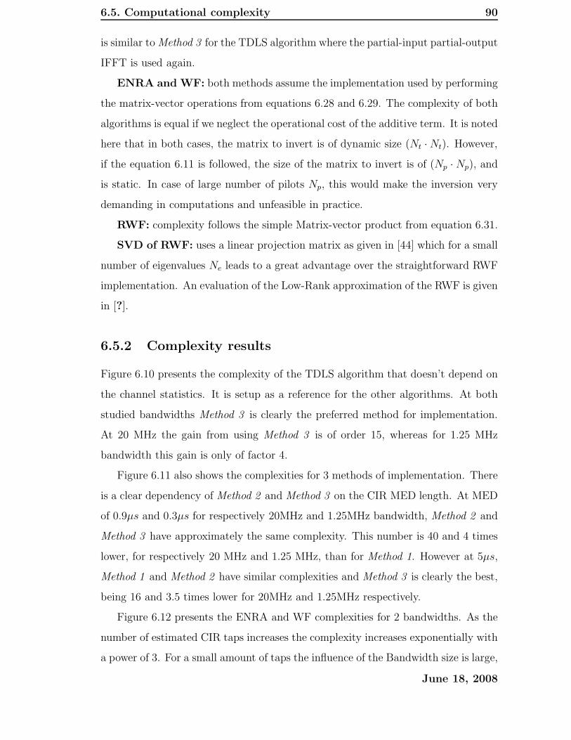
6.5. Computational complexity 90
is similar to Method 3 for the TDLS algorithm where the partial-input partial-output
IFFT is used again.
ENRA and WF: both methods assume the implementation used by performing
the matrix-vector operations from equations 6.28 and 6.29. The complexity of both
algorithms is equal if we neglect the operational cost of the additive term. It is noted
here that in both cases, the matrix to invert is of dynamic size (Nt ·Nt). However,
if the equation 6.11 is followed, the size of the matrix to invert is of (Np ·Np), and
is static. In case of large number of pilots Np, this would make the inversion very
demanding in computations and unfeasible in practice.
RWF: complexity follows the simple Matrix-vector product from equation 6.31.
SVD of RWF: uses a linear projection matrix as given in [44] which for a small
number of eigenvalues Ne leads to a great advantage over the straightforward RWF
implementation. An evaluation of the Low-Rank approximation of the RWF is given
in [?].
6.5.2 Complexity results
Figure 6.10 presents the complexity of the TDLS algorithm that doesn’t depend on
the channel statistics. It is setup as a reference for the other algorithms. At both
studied bandwidths Method 3 is clearly the preferred method for implementation.
At 20 MHz the gain from using Method 3 is of order 15, whereas for 1.25 MHz
bandwidth this gain is only of factor 4.
Figure 6.11 also shows the complexities for 3 methods of implementation. There
is a clear dependency of Method 2 and Method 3 on the CIR MED length. At MED
of 0.9µs and 0.3µs for respectively 20MHz and 1.25MHz bandwidth, Method 2 and
Method 3 have approximately the same complexity. This number is 40 and 4 times
lower, for respectively 20 MHz and 1.25 MHz, than for Method 1. However at 5µs,
Method 1 and Method 2 have similar complexities and Method 3 is clearly the best,
being 16 and 3.5 times lower for 20MHz and 1.25MHz respectively.
Figure 6.12 presents the ENRA and WF complexities for 2 bandwidths. As the
number of estimated CIR taps increases the complexity increases exponentially with
a power of 3. For a small amount of taps the influence of the Bandwidth size is large,
June 18, 2008
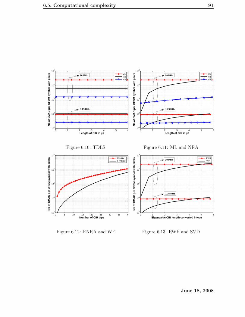
6.5. Computational complexity 91
0 1 2 3 4 5 610
2
103
104
105
106
Length of CIR in µs
Nb
of C
MA
C p
er O
FD
M s
ymbo
l with
pilo
ts
M1M2M3
20 MHz
1.25 MHz
Figure 6.10: TDLS
0 1 2 3 4 5 610
2
103
104
105
106
Length of CIR in µsN
b of
CM
AC
per
OF
DM
sym
bol w
ith p
ilots
M1M2M3
20 MHz
1.25 MHz
Figure 6.11: ML and NRA
0 5 10 15 20 25 30 35 4010
2
103
104
105
106
Number of CIR taps
Nb
of C
MA
C p
er O
FD
M s
ymbo
l with
pilo
ts
20MHz1.25MHz
Figure 6.12: ENRA and WF
0 1 2 3 4 5 610
2
103
104
105
106
Eigenvalue/CIR length converted into µs
Nb
of C
MA
C p
er O
FD
M s
ymbo
l with
pilo
ts
RWFSVD
20 MHz
1.25 MHz
Figure 6.13: RWF and SVD
June 18, 2008

6.6. Conclusion 92
however as the number of taps increases the influence of the Bandwidth tends to be
reduced.
Figure 6.13 shows the complexity gain by using an SVD approach on the RWF.
The complexity gain is especially large for cases of low number of eigenvalues. When
using an SVD of the RWF the number of eigenvalues is largely correlated to the CIR
MED (see appendix C.6). At equivalent length of 1µs, the SVD implementation
is approx 6 and 3.4 times less complex than the RWF for 20MHz and 1.25MHz
respectively.
6.6 Conclusion
This chapter is an in depth study of frequency direction linear PACE algorithms.
A framework has been provided for a choice of interpolation algorithm in upcoming
OFDM based standards. In a first step a classification has been carried out from a
state of the art survey, showing that the linear solutions provided in literature can
be classified into time and frequency domain approaches. They are also classified
according to their a priori assumptions. A comparison of classical linear PACE
OFDM algorithms using a generalized estimator formulation has been presented. It
has been shown that each algorithm is a particular case of this estimator and depends
on the a priori channel information taken into account. Analysis and simulation
results are first given for a sample-spaced channel and Full Bandwidth, showing
that the performance is improved as the amount of a priori information increases.
The effects of introducing virtual subcarriers as well as a non-sample-spaced channel
are then studied. When Partial Bandwidth is used, the TDLS and ML algorithms
suffer from severe ill-conditioned matrices and cannot be used as such if the number
of virtual subcarriers is too large.
When discarding the leakage effect due to non sample spaced CIR and when
looking at SNR values in the range -10dB to 10 dB, the optimized partial-input
partial-output FFT based implementation of the NRA has the lowest complexity and
doesn’t deteriorate the CTF estimate significantly. However, at SNR values above
10dB the leakage effect renders the NRA solution unusable and only the ENRA, WF
June 18, 2008

6.6. Conclusion 93
and RWF for non sample spaced channels should be used. The complexity of this
RWF can be lowered by SVD based low rank approximation and is especially efficient
for ”short” channel profiles with MED in the order 1 µs. However at MED of around
4-5 µs very little computational gain can be gained by this low rank technique as the
number of singular values with significant value is quite high. Therefore for larger
bandwidths of 20 MHz the complexity of the RWF is fairly high.
On the other hand, the true WF and the ENRA provide lower complexities than
the RWF even for channels with up to 40 taps and MED of 4-5 µs. The WF and
ENRA clearly give the best performances as long as the CIR delays are accurate.
From this analysis we conclude that the WF and ENRA are the most suitable
algorithms from both performance and complexity point of view as long as accurate
CIR delays are provided. CIR delay tracking for OFDM has been studied in [70,75].
The accuracy and complexity of this methods depend on richness and the variability
over time of the delay subspace. In practice it is therefore not trivial to determine
the best solution. The RWF will ”work” in all cases, within the assumptions and
gives a fixed degradation from known channel performance, depending on the MED
of the CIR. The ENRA/WF solutions will be able to perform up to 1-2 dB better
than this depending on the channel scenario but their reliability is determined by
the CIR delay estimate accuracy. In a first release of LTE the RWF solution with
low rank precalculated filter is therefore recommended. For further performance
improvements, low complex and accurate delay tracking will be needed.
June 18, 2008
Chapter 7
Pilot pattern and pilot density
evaluation
7.1 Introduction
In order to perform coherent detection, reliable channel estimates are required.
When dealing with a PACE OFDM based system, these initial estimates are ob-
tained from transmitting known data symbols, also called pilot symbols. As previ-
ously shown in chapter 5 and chapter 6, the receiver interpolates from the initial
channel information at the pilot position to obtain the channel estimate for the data
signal. One of the classical problems of designing a PACE-OFDM system is to de-
cide where and how often to insert pilot symbols. As the pilots are pure overhead
consuming system resources, the spacing should be large enough not to increase this
overhead too much. At the same time the spacing should be small enough to enable
reliable channel estimates.
This chapter proposes several objectives. First, we propose to investigate the
different interpolation algorithms robustness against varying pilot spacing, also in
the case of aliasing due to under-sampled channels. Secondly, a methodology to be
used for pilot design is discussed based on a tradeoff between algorithmic complexity,
pilot overhead and MSE performance. Finally, a proposal for the pilot distribution
and density is made for the studied downlink LTE scenario.
The Nyquist-Shannon sampling theorem is a fundamental result in the field of
94
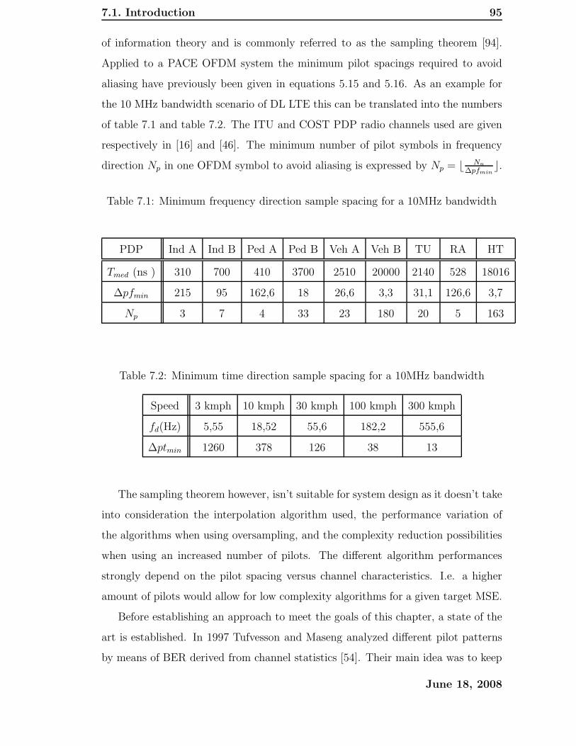
7.1. Introduction 95
of information theory and is commonly referred to as the sampling theorem [94].
Applied to a PACE OFDM system the minimum pilot spacings required to avoid
aliasing have previously been given in equations 5.15 and 5.16. As an example for
the 10 MHz bandwidth scenario of DL LTE this can be translated into the numbers
of table 7.1 and table 7.2. The ITU and COST PDP radio channels used are given
respectively in [16] and [46]. The minimum number of pilot symbols in frequency
direction Np in one OFDM symbol to avoid aliasing is expressed by Np = ⌊ Nu
∆pfmin⌋.
Table 7.1: Minimum frequency direction sample spacing for a 10MHz bandwidth
PDP Ind A Ind B Ped A Ped B Veh A Veh B TU RA HT
Tmed (ns ) 310 700 410 3700 2510 20000 2140 528 18016
∆pfmin 215 95 162,6 18 26,6 3,3 31,1 126,6 3,7
Np 3 7 4 33 23 180 20 5 163
Table 7.2: Minimum time direction sample spacing for a 10MHz bandwidth
Speed 3 kmph 10 kmph 30 kmph 100 kmph 300 kmph
fd(Hz) 5,55 18,52 55,6 182,2 555,6
∆ptmin 1260 378 126 38 13
The sampling theorem however, isn’t suitable for system design as it doesn’t take
into consideration the interpolation algorithm used, the performance variation of
the algorithms when using oversampling, and the complexity reduction possibilities
when using an increased number of pilots. The different algorithm performances
strongly depend on the pilot spacing versus channel characteristics. I.e. a higher
amount of pilots would allow for low complexity algorithms for a given target MSE.
Before establishing an approach to meet the goals of this chapter, a state of the
art is established. In 1997 Tufvesson and Maseng analyzed different pilot patterns
by means of BER derived from channel statistics [54]. Their main idea was to keep
June 18, 2008

7.1. Introduction 96
the number of pilots to a minimum and thereby reduce the system overhead. Hoeher
used a rectangular equispaced pilot grid [63] in his fundamental 2D versus 2 times
1D interpolation comparison. Negi proved analytically in [71] that the optimal
selection of pilot symbols was based on equispaced non-clustered pilot symbols.
Here, it is noted that he assumed a full bandwidth OFDM system (with Nu =
Nfft) and the TDLS algorithm for his work. In the case of partial bandwidth
OFDM with virtual subcarriers (where Nu < Nfft), Morelli then showed in [79] that
equispaced pilots is not an optimal distribution. He showed better MSE performance
with non-uniformly spaced pilots. However this behavior is channel specific and
exhaustive search is needed for each channel realization to obtain the optimal pilot
spacing arrangement. Gracia proposed in [82] a novel hexagonal pilot geometry
optimal in sampling efficiency. His work is limited to the case of an optimal 2D
Wiener interpolator and purely relies on the sampling theorem. Zhang proposed a
novel method of deciding on the number of pilots in [83]. This method is based
on analytical uncoded BER calculation as a function of channel statistics and lacks
effect of forward error coding (such a Turbo Coding), thereby lacking usefulness for
a practical system design. Finally, Choi proposed the optimum pilot pattern that
minimizes the MSE for given pilot density and channel statistics in [84]. It was
demonstrated that a diamond pilot shape provides estimation performance better
than any other shape. Also he stated that the optimum pilot spacing was directly
a function of the PDP and Doppler spectrum.
An analytical model of the received OFDM baseband signal has been derived in
section 2.2 and is used to further derive a loss model. This model separates channel
estimation inaccuracy, pilot overhead and ICI losses. A classical OFDM single tap
equalizer is assumed throughout this chapter. Channel estimation efficiency is there-
fore a tradeoff between pilot spacing and estimation accuracy and has previously
been studied in OFDM with ICI [87], and advanced receivers have been derived to
cope with ICI. However, these receiver types are excessively demanding in compu-
tational complexity [88]. From the above, it may be seen that there are three main
mechanisms that will cause a spectral efficiency loss in the system performance:
Ltotal = Lalgo + Lpilot + Lici. (7.1)
June 18, 2008

7.2. Channel estimation approach 97
In 7.1 the loss is measured in dB relative to optimal performance. Lalgo represents the
loss due to the inaccuracy of the channel transfer function estimation, and depends
on the algorithm as well as the pilot pattern used. Lpilot is the loss due to overhead of
pilot symbols, which will decrease the amount of available user information symbols.
Lpilot is solely dependent on the pilot scheme. Finally, Lici is the loss due to ICI
from Doppler distortion of the transmitted signal at high speeds.
In the rest of this chapter we will first establish the channel estimation strategy
to be adopted in a LTE receiver based on previous work stated in the state of the art.
Secondly the behavior of the frequency and time direction interpolation algorithm
will be be investigated. A subset of proposed algorithms are selected for frequency
direction interpolation from the early study in chapter 6 and time direction from
the work in [52]. Based on this we will end up with a pilot scheme proposal for the
downlink LTE SISO scenario.
7.2 Channel estimation approach
Form the results of Hoeher in [63] the 2D interpolation problem is separated into
2 times 1D successive interpolations, as the loss by adopting this method is quasi
negligible and the computational complexity gains considerable. An adaptive pilot
structure would lead to better performance, however such a solution is not desirable
as it would lead to increased signalling complexity. Therefore, a fixed ”worst-case”
design is adopted with one single pilot scheme covering all channel scenarios. The
optimum pilot pattern has been shown to be the ”diamond” structure in [84]. Un-
fortunately the LTE frame structure doesn’t allow such an accurate pattern. In
figure 7.2 we approximate the diamond structure and use the proposed patterns
for performance evaluation. As mobile PACE OFDM systems have high latency
requirements, the pilot span available in time direction is considerably limited. It
follows naturally to perform a stepwise interpolation by starting with the frequency
direction interpolation. Then from these full bandwidth estimates at the OFDM
symbols containing pilots, we interpolate in a second step in the time direction as
shown in figure 7.1.
June 18, 2008
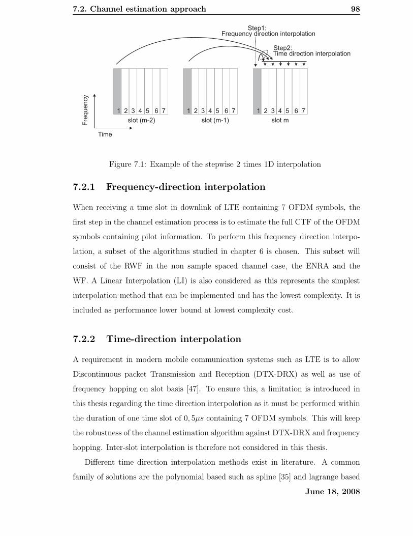
7.2. Channel estimation approach 98
Time
Fre
qu
en
cy
slot mslot (m-1)slot (m-2)
Frequency direction interpolationStep1:
Step2:Time direction interpolation
1 2 3 4 5 6 7 1 2 3 4 5 6 7 1 2 3 4 5 6 7
Figure 7.1: Example of the stepwise 2 times 1D interpolation
7.2.1 Frequency-direction interpolation
When receiving a time slot in downlink of LTE containing 7 OFDM symbols, the
first step in the channel estimation process is to estimate the full CTF of the OFDM
symbols containing pilot information. To perform this frequency direction interpo-
lation, a subset of the algorithms studied in chapter 6 is chosen. This subset will
consist of the RWF in the non sample spaced channel case, the ENRA and the
WF. A Linear Interpolation (LI) is also considered as this represents the simplest
interpolation method that can be implemented and has the lowest complexity. It is
included as performance lower bound at lowest complexity cost.
7.2.2 Time-direction interpolation
A requirement in modern mobile communication systems such as LTE is to allow
Discontinuous packet Transmission and Reception (DTX-DRX) as well as use of
frequency hopping on slot basis [47]. To ensure this, a limitation is introduced in
this thesis regarding the time direction interpolation as it must be performed within
the duration of one time slot of 0, 5µs containing 7 OFDM symbols. This will keep
the robustness of the channel estimation algorithm against DTX-DRX and frequency
hopping. Inter-slot interpolation is therefore not considered in this thesis.
Different time direction interpolation methods exist in literature. A common
family of solutions are the polynomial based such as spline [35] and lagrange based
June 18, 2008
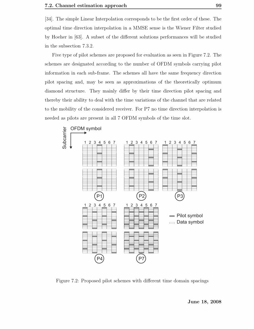
7.2. Channel estimation approach 99
[34]. The simple Linear Interpolation corresponds to be the first order of these. The
optimal time direction interpolation in a MMSE sense is the Wiener Filter studied
by Hoeher in [63]. A subset of the different solutions performances will be studied
in the subsection 7.3.2.
Five type of pilot schemes are proposed for evaluation as seen in Figure 7.2. The
schemes are designated according to the number of OFDM symbols carrying pilot
information in each sub-frame. The schemes all have the same frequency direction
pilot spacing and, may be seen as approximations of the theoretically optimum
diamond structure. They mainly differ by their time direction pilot spacing and
thereby their ability to deal with the time variations of the channel that are related
to the mobility of the considered receiver. For P7 no time direction interpolation is
needed as pilots are present in all 7 OFDM symbols of the time slot.
P1 P2 P3
P4 P7
OFDM symbol
Subcarr
ier
1 2 3 4 5 6 7 1 2 3 4 5 6 7 1 2 3 4 5 6 7
1 2 3 4 5 6 7 1 2 3 4 5 6 7
Pilot symbol
Data symbol
Figure 7.2: Proposed pilot schemes with different time domain spacings
June 18, 2008
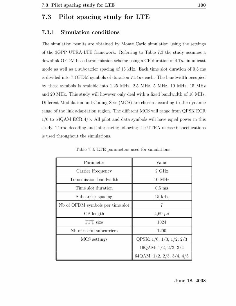
7.3. Pilot spacing study for LTE 100
7.3 Pilot spacing study for LTE
7.3.1 Simulation conditions
The simulation results are obtained by Monte Carlo simulation using the settings
of the 3GPP UTRA-LTE framework. Referring to Table 7.3 the study assumes a
downlink OFDM based transmission scheme using a CP duration of 4.7µs in unicast
mode as well as a subcarrier spacing of 15 kHz. Each time slot duration of 0,5 ms
is divided into 7 OFDM symbols of duration 71.4µs each. The bandwidth occupied
by these symbols is scalable into 1.25 MHz, 2.5 MHz, 5 MHz, 10 MHz, 15 MHz
and 20 MHz. This study will however only deal with a fixed bandwidth of 10 MHz.
Different Modulation and Coding Sets (MCS) are chosen according to the dynamic
range of the link adaptation region. The different MCS will range from QPSK ECR
1/6 to 64QAM ECR 4/5. All pilot and data symbols will have equal power in this
study. Turbo decoding and interleaving following the UTRA release 6 specifications
is used throughout the simulations.
Table 7.3: LTE parameters used for simulations
Parameter Value
Carrier Frequency 2 GHz
Transmission bandwidth 10 MHz
Time slot duration 0,5 ms
Subcarrier spacing 15 kHz
Nb of OFDM symbols per time slot 7
CP length 4,69 µs
FFT size 1024
Nb of useful subcarriers 1200
MCS settings QPSK: 1/6, 1/3, 1/2, 2/3
16QAM: 1/2, 2/3, 3/4
64QAM: 1/2, 2/3, 3/4, 4/5
June 18, 2008
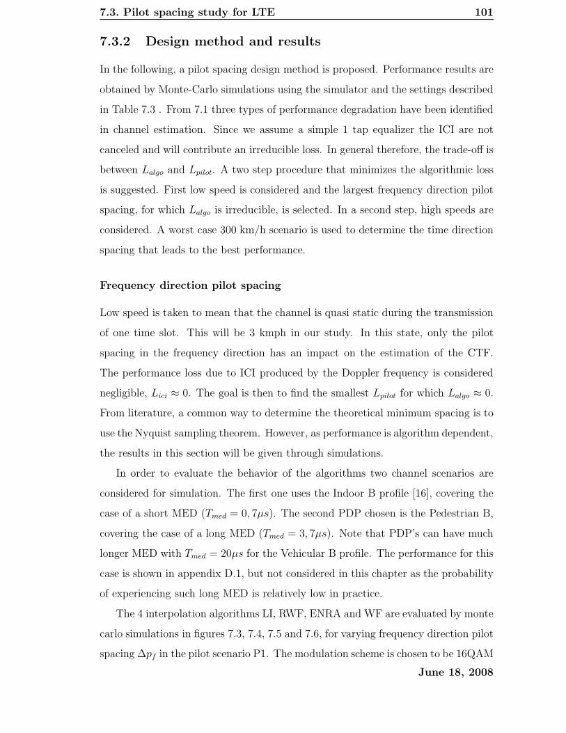
7.3. Pilot spacing study for LTE 101
7.3.2 Design method and results
In the following, a pilot spacing design method is proposed. Performance results are
obtained by Monte-Carlo simulations using the simulator and the settings described
in Table 7.3 . From 7.1 three types of performance degradation have been identified
in channel estimation. Since we assume a simple 1 tap equalizer the ICI are not
canceled and will contribute an irreducible loss. In general therefore, the trade-off is
between Lalgo and Lpilot. A two step procedure that minimizes the algorithmic loss
is suggested. First low speed is considered and the largest frequency direction pilot
spacing, for which Lalgo is irreducible, is selected. In a second step, high speeds are
considered. A worst case 300 km/h scenario is used to determine the time direction
spacing that leads to the best performance.
Frequency direction pilot spacing
Low speed is taken to mean that the channel is quasi static during the transmission
of one time slot. This will be 3 kmph in our study. In this state, only the pilot
spacing in the frequency direction has an impact on the estimation of the CTF.
The performance loss due to ICI produced by the Doppler frequency is considered
negligible, Lici ≈ 0. The goal is then to find the smallest Lpilot for which Lalgo ≈ 0.
From literature, a common way to determine the theoretical minimum spacing is to
use the Nyquist sampling theorem. However, as performance is algorithm dependent,
the results in this section will be given through simulations.
In order to evaluate the behavior of the algorithms two channel scenarios are
considered for simulation. The first one uses the Indoor B profile [16], covering the
case of a short MED (Tmed = 0, 7µs). The second PDP chosen is the Pedestrian B,
covering the case of a long MED (Tmed = 3, 7µs). Note that PDP’s can have much
longer MED with Tmed = 20µs for the Vehicular B profile. The performance for this
case is shown in appendix D.1, but not considered in this chapter as the probability
of experiencing such long MED is relatively low in practice.
The 4 interpolation algorithms LI, RWF, ENRA and WF are evaluated by monte
carlo simulations in figures 7.3, 7.4, 7.5 and 7.6, for varying frequency direction pilot
spacing ∆pf in the pilot scenario P1. The modulation scheme is chosen to be 16QAM
June 18, 2008
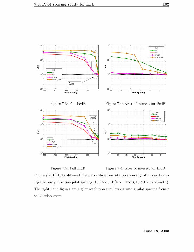
7.3. Pilot spacing study for LTE 102
010020030040050010
−3
10−2
10−1
100
Pilot Spacing
BE
R
KCLIWFENRARWF (NSS)
Area ofinterest
Figure 7.3: Full PedB
5101520253010
−3
10−2
10−1
100
Pilot Spacing
BE
R
KCLIWFENRARW (NSS)
Figure 7.4: Area of interest for PedB
010020030040050010
−3
10−2
10−1
100
Pilot Spacing
BE
R
KCLIWFENRARWF (NSS)
Area ofinterest
Figure 7.5: Full IndB
5101520253010
−3
10−2
10−1
100
Pilot Spacing
BE
R
KCLIWFENRARW (NSS)
Figure 7.6: Area of interest for IndB
Figure 7.7: BER for different Frequency direction interpolation algorithms and vary-
ing frequency direction pilot spacing (16QAM, Eb/No = 17dB, 10 MHz bandwidth).
The right hand figures are higher resolution simulations with a pilot spacing from 2
to 30 subcarriers.
June 18, 2008

7.3. Pilot spacing study for LTE 103
and the uncoded BER versus ∆pf are chosen as evaluation criterion.
The pilot spacings simulated are ∆pf ∈ {2, 4, 8, 16, 32, 64, 128, 256, 512} in figure
7.3 and 7.5. When looking into the areas of interest with reduced performance
degradation, we notice that the pilot spacing is low. The pilot spacing resolution is
then increased in the area of interest for the right hand figures 7.4 and 7.6. In the
case of PedB it is observed that the ENRA and WF are robust to the pilot spacing
variation whereas LI and even RWF quickly degrade in BER as the pilot spacing
is increased. In the case of IndB it is observed that all the algorithms seem robust
to a variation of pilot spacing in the range of [2 30]. The LI has clearly the worst
BER as expected. We also note that for low pilot spacing of ∆pf ≤ 10, the RWF
performs quasi optimally. For further results a pilot spacing of ∆pf = 8 is chosen
as average value.
Time direction pilot spacing
At high velocities the channel varies significantly during the transmission of one
time slot. In this state, Lici > 0, since with a classical single tap equalizer the ICI
cannot be canceled. However, by choosing pilot scheme P7, pilots will be present in
each OFDM symbol and it is possible to obtain Lalgo ≈ 0 without the use of time
direction interpolation. Consequently, by looking at Packet Error Rate (PER) we
can quantify the degradation due to ICI. The PER for three different MCS and two
different speeds is shown in Figure 7.8.
Assuming a link adaptation operating point at a PER of 20 %, the loss due to
ICI is given in Table 7.4. At 100 kmph the loss due to ICI is minimal, whereas it
can be as high as 1,5 dB at 300 kmph for 64QAM ECR 2/3.
Table 7.4: Performance loss due to ICI and estimation inaccuracy at 20 % PER
Velocity 100 kmph 300 kmph
QPSK, ECR 2/3 0,1 dB 0,3 dB
16QAM, ECR 2/3 0,4 dB 0,5 dB
64QAM, ECR 2/3 0,5 dB 1,5 dB
June 18, 2008
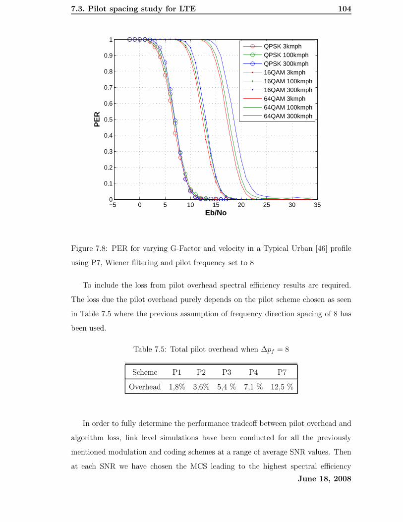
7.3. Pilot spacing study for LTE 104
−5 0 5 10 15 20 25 30 350
0.1
0.2
0.3
0.4
0.5
0.6
0.7
0.8
0.9
1
Eb/No
PE
R
QPSK 3kmphQPSK 100kmphQPSK 300kmph16QAM 3kmph16QAM 100kmph16QAM 300kmph64QAM 3kmph64QAM 100kmph64QAM 300kmph
Figure 7.8: PER for varying G-Factor and velocity in a Typical Urban [46] profile
using P7, Wiener filtering and pilot frequency set to 8
To include the loss from pilot overhead spectral efficiency results are required.
The loss due the pilot overhead purely depends on the pilot scheme chosen as seen
in Table 7.5 where the previous assumption of frequency direction spacing of 8 has
been used.
Table 7.5: Total pilot overhead when ∆pf = 8
Scheme P1 P2 P3 P4 P7
Overhead 1,8% 3,6% 5,4 % 7,1 % 12,5 %
In order to fully determine the performance tradeoff between pilot overhead and
algorithm loss, link level simulations have been conducted for all the previously
mentioned modulation and coding schemes at a range of average SNR values. Then
at each SNR we have chosen the MCS leading to the highest spectral efficiency
June 18, 2008
7.3. Pilot spacing study for LTE 105
−10 0 10 20 30 400
0.5
1
1.5
2
2.5
3
3.5
4
SNR (dB)
Spe
ctra
l Effi
cien
cy (
b/s/
Hz)
P1 3kmphP1 300kmphP2 300kpmhP3 300kmphP4 300kpmhP7 300kmph
Figure 7.9: Spectral Efficiency in DL LTE, Typical Urban [46], 10MHz
so as to obtain an ideal link adaptation curve. Because of the large bandwidth
assumption, which stabilizes the SNR, this result is almost identical to real time
domain link adaptation as shown in [95]. The link curves for the different pilot
schemes and different speeds are shown in Figure 7.9, including the low speed case
with P1. This latter shows the upper performance bound achievable for a LTE
system, as in this case Lici ≈ 0 and Lalgo ≈ 0, leaving only degradation to pilot
overhead of 1.8%.
At 300 kmph there is similar Spectral Efficiency using the pilot schemes P2, P3,
P4 and P7 with SNR ranging from -10 dB up to 20dB. However when going above 20
dB of SNR P2 and P7 perform with around 0,3 bits per second per Hertz less spectral
efficiency. In the case of P1 at 300kmph the achievable efficiency is limited to around
17 % of the low speed performance. The choice of one single pilot scheme to cover
all channel scenarios boils down to choosing between P2 and P3. P2 has a lower
high speed worst case performance in the area of high SNR compared to P3. From
June 18, 2008

7.4. Conclusion 106
the requirements of [2] the LTE system should be optimized for low mobile speed
but also support high mobile speed. Therefore the scheme P2 will be chosen, as it
optimizes the systems at low speed by having less pilot overhead but still provides
sufficient performance at high speeds. This will give a time direction spacing set
to 3,5 OFDM symbols in average and with the frequency direction spacing set to 8
subcarriers, corresponding respectively to 0.25 ms and 120 kHz. The pilot overhead
will be 3.6%.
7.4 Conclusion
The purpose of this chapter has been to give an estimate of performance degradation
due to channel estimation as well as to propose a suitable pilot distribution in a
downlink context. This work has differed from previous similar studies as it targets
the UTRA-LTE context, with practical constraints considered. Notably, these are
low latency, optimized low speed performance, improved spectral efficiency, low
terminal complexity, and support for high mobile speed. Different objectives were
proposed.
First the robustness of different interpolation algorithms against variation of
pilot spacing was investigated. In the frequency direction the RWF and LI turned
out to be very sensitive to minor changes in pilot spacing in the case of PDP with
long delays. When the delays are short, sensitivity to varying frequency direction
pilots spacing is quasi-insignificant. The ENRA and WF using a priori knowledge
of tap delay location turned out to be very robust to pilot spacing variation even
in the case of large PDP delays. In the time direction the importance of algorithm
choice is of little relevance in the low speed scenario as the channel is quasi-static
over the duration of one time slot. At very high speeds up to 300 kmph worst-case
scenario, LI can still be used but leads to performance degradation at high SNR
using a 64QAM modulation. The overall importance of time direction interpolation
is however reduced as ICI is irreducible when using a classical OFDM 1 tap equalizer.
Also DRX-DTX, and latency requirements force the estimation to be done within
the duration of one time slot estimation, and inter-slot interpolation is undesirable.
June 18, 2008

7.4. Conclusion 107
Secondly, a methodology for pilot distribution design based on LTE system spe-
cific requirements has been proposed, leading to a two step strategy. Step one de-
termines the largest frequency direction pilot spacing that keeps the estimation loss
low. This is done in a low speed scenario where the channel is stationary during one
time slot transmission. Step two evaluates the largest time direction pilot spacing
leading to acceptable performance in a worst-case 300 kmph high speed scenario.
Thirdly, one fixed pilot pattern is proposed for downlink LTE from the previously
derived method. The pilot scheme will have an overhead of 3,6 %, cover all consid-
ered channel scenarios and will have support for high mobile speeds up to 300kmph.
Spectral efficiency results are shown for a wide range of proposed modulation and
coding schemes going from -10 dB to +40 dB SNR, and confirm the validity of the
proposed distribution.
Finally, future perspectives would be to investigate the feasibility of frequency di-
rection interpolation algorithm using a priori tap delay knowledge, thereby allowing
very low pilot overhead. Also the scenario of single frequency network MBMS trans-
mitting continuous data would increase the importance of time averaging, filtering
and predictive algorithms.
June 18, 2008

Chapter 8
Self-induced interference
cancelation
8.1 Introduction
One of the main assumptions for the studies carried out in chapters 5, 6 and 7
is to assume a PDP MED duration smaller than the CP duration of the OFDM
symbol. Unfortunately this assumption doesn’t always hold true in which case
the receiver signal quality is degraded by the resulting interference. The classical
characterization of self induced interference in OFDM is modeled by Inter OFDM-
Symbol Interference (ISI) and Inter Carrier Interference (ICI). The insertion of the
CP cancels the interference as long as the CP is sufficiently long, but with larger
fading delays, the CP can only mitigate this interference. A serious drawback of
introducing a CP is the linear reduction of spectral efficiency of the system by a
factor of Tg
Tofdm, as the CP is pure overhead and doesn’t contain any additional data
information. Another source of ICI is the time variation of the radio channel when
appreciable changes occur during one symbol period as studied in [22], [23] and [24].
The effect of ICI due to time variation of the radio channel will not be the focus of
this chapter. Proposal of an adaptive CP length technique has been made in [98].
The downside of this proposal is the increased system signalling complexity when
the solution has to adjust to different radio scenarios as the receiver experiences
different radio propagation environments.
108
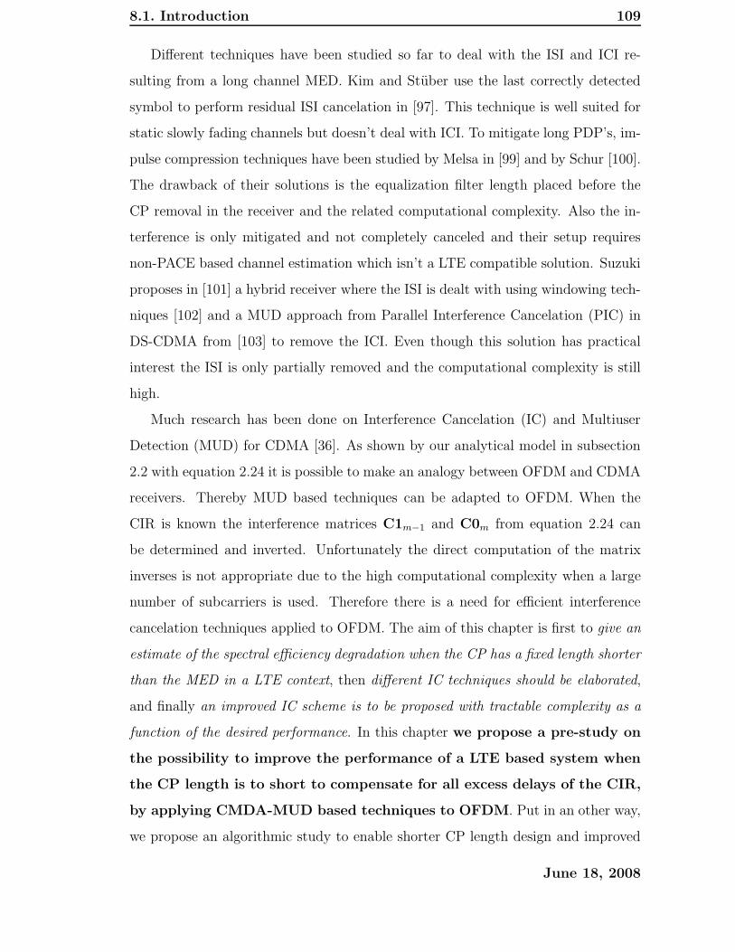
8.1. Introduction 109
Different techniques have been studied so far to deal with the ISI and ICI re-
sulting from a long channel MED. Kim and Stuber use the last correctly detected
symbol to perform residual ISI cancelation in [97]. This technique is well suited for
static slowly fading channels but doesn’t deal with ICI. To mitigate long PDP’s, im-
pulse compression techniques have been studied by Melsa in [99] and by Schur [100].
The drawback of their solutions is the equalization filter length placed before the
CP removal in the receiver and the related computational complexity. Also the in-
terference is only mitigated and not completely canceled and their setup requires
non-PACE based channel estimation which isn’t a LTE compatible solution. Suzuki
proposes in [101] a hybrid receiver where the ISI is dealt with using windowing tech-
niques [102] and a MUD approach from Parallel Interference Cancelation (PIC) in
DS-CDMA from [103] to remove the ICI. Even though this solution has practical
interest the ISI is only partially removed and the computational complexity is still
high.
Much research has been done on Interference Cancelation (IC) and Multiuser
Detection (MUD) for CDMA [36]. As shown by our analytical model in subsection
2.2 with equation 2.24 it is possible to make an analogy between OFDM and CDMA
receivers. Thereby MUD based techniques can be adapted to OFDM. When the
CIR is known the interference matrices C1m−1 and C0m from equation 2.24 can
be determined and inverted. Unfortunately the direct computation of the matrix
inverses is not appropriate due to the high computational complexity when a large
number of subcarriers is used. Therefore there is a need for efficient interference
cancelation techniques applied to OFDM. The aim of this chapter is first to give an
estimate of the spectral efficiency degradation when the CP has a fixed length shorter
than the MED in a LTE context, then different IC techniques should be elaborated,
and finally an improved IC scheme is to be proposed with tractable complexity as a
function of the desired performance. In this chapter we propose a pre-study on
the possibility to improve the performance of a LTE based system when
the CP length is to short to compensate for all excess delays of the CIR,
by applying CMDA-MUD based techniques to OFDM. Put in an other way,
we propose an algorithmic study to enable shorter CP length design and improved
June 18, 2008

8.2. Analysis 110
interference reduction in OFDM systems, by means of IC in the receiver.
Section 8.2 sets the scene by introducing ISI and ICI problematic, as well as
showing the impact of a long MED channel profiles on spectral efficiency in a short
CP scenario. Different classical IC techniques are also presented and performance
is given in a LTE context. Section 8.3 discusses the novel LCIC algorithm. Section
8.4 evaluates the feasibility of the LCIC algorithm in LTE through a complexity
analysis. Finally section 8.5 discusses the obtained results.
8.2 Analysis
As stated in chapter 4, it is beneficial to only have one fixed CP length in a OFDM
system. Thereby reducing the system signalling complexity and the related infor-
mation overhead to be transmitted instead of data information. When only one CP
length is to be chosen for a system, it is not possible both to have a short CP to
reduce the CP overhead, and a long CP to limit the interference created by long
PDP delays. A tradeoff solution must be chosen. In figure 8.1 the spectral efficiency
versus SNR is shown in the case of three channel PDP, namely Typical Urban (TU),
Vehicular B (VehB) and Hilly Terrain (HT) (presented in Appendix A). The ICI
and ISI resulting from a channel MED longer than the CP length of 4, 69µs degrades
tremendously the achievable performance. At low SNR the degradation is not so
significant, however at high SNR a performance floor is observed for VehB and HT,
where the spectral efficiency is limited to 1,9 and 2,4 Bit/s/Hz respectively.
The idea is to apply DS-CDMA MUD principles to OFDM when interference
such as ISI and ICI corrupts the signal. In a first step we recall, from section 2.2,
equation 2.24:
zm = C0mdm + C1m−1dm−1 + ΨHmwm
and equation 2.25:
zm = zS,m + zICI,m + zISI,m + ΨHmwm.
The dimensions of C0m are (Nu.Nu), which gives for a LTE 20MHz scenario,
Nu = 1200. The inversion of such a large matrix is computationally prohibitive
June 18, 2008
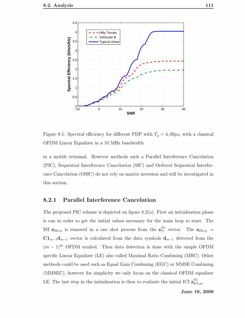
8.2. Analysis 111
−10 0 10 20 30 400
0.5
1
1.5
2
2.5
3
3.5
4
4.5
SNR
Spe
ctra
l Effi
cien
cy (
bits
/s/H
z)
Hilly TerrainVehicular BTypical Urban
Figure 8.1: Spectral efficiency for different PDP with Tg = 4, 69µs, with a classical
OFDM Linear Equalizer in a 10 MHz bandwidth
in a mobile terminal. However methods such a Parallel Interference Cancelation
(PIC), Sequential Interference Cancelation (SIC) and Ordered Sequential Interfer-
ence Cancelation (OSIC) do not rely on matrix inversion and will be investigated in
this section.
8.2.1 Parallel Interference Cancelation
The proposed PIC scheme is depicted on figure 8.2(a). First an initialization phase
is run in order to get the initial values necessary for the main loop to start. The
ISI zISI,m is removed in a one shot process from the z(0)m vector. The zISI,m =
C1m−1dm−1 vector is calculated from the data symbols dm−1 detected from the
(m − 1)th OFDM symbol. Then data detection is done with the simple OFDM
specific Linear Equalizer (LE) also called Maximal Ratio Combining (MRC). Other
methods could be used such as Equal Gain Combining (EGC) or MMSE Combining
(MMSEC), however for simplicity we only focus on the classical OFDM equalizer
LE. The last step in the initialization is then to evaluate the initial ICI z(0)ICI,m.
June 18, 2008

8.2. Analysis 112
Once the initialization is complete the iterative phase can start. In a first step,
the ICI z(s)ICI,mis removed from the ISI free received signal zm. In a second step,
the symbol detection is performed using the LE with known C0S,m (containing the
diagonal elements of C0m) equivalent to the CTF. In a third step, symbol decision
is performed based on minimal Euclidean distance. Finally the fourth step, tests
if the number of iterations s is larger than the maximal number of iterations S. If
s ≥ S the loop ends and the latest updated d(s)m is used as detected data symbols,
else if s < S the loop continues and the ICI is updated with newly detected symbol
vector d(s)m .
8.2.2 Sequential Interference Cancelation
The proposed SIC scheme is depicted on figure 8.2(b). The initialization phase for
both SIC and OSIC schemes is the same as for the PIC scheme. The iterative phase
is however different. It is built as two concatenated loops. The inner loop removes
ICI z(s)ICI,m[k] row by row considering only one subcarrier at the time for each iteration
k. At each inner iteration a new symbol detection is performed giving d(s)m [k]. This
symbol is then used to update the ICI if the symbol has changed from the previous
outer iteration. This entire procedure is repeated until the iteration counter k is
incremented to Nu. When k = Nu the outer loop iteration counter s is incremented
by 1. This procedure is then repeated until the outer loop counter is equal to S,
where both loops end and the latest updated d(s)m is used as detected data symbols.
The proposed OSIC scheme is depicted on figure 8.2(c). The OSIC scheme is
almost identical with the SIC scheme with the difference that it orders the sequence
of received signal subcarriers z(s)ICI,m[k] at the beginning in each iteration of the outer
loop. Then at the end of both loops the original subcarrier order is restored.
June 18, 2008
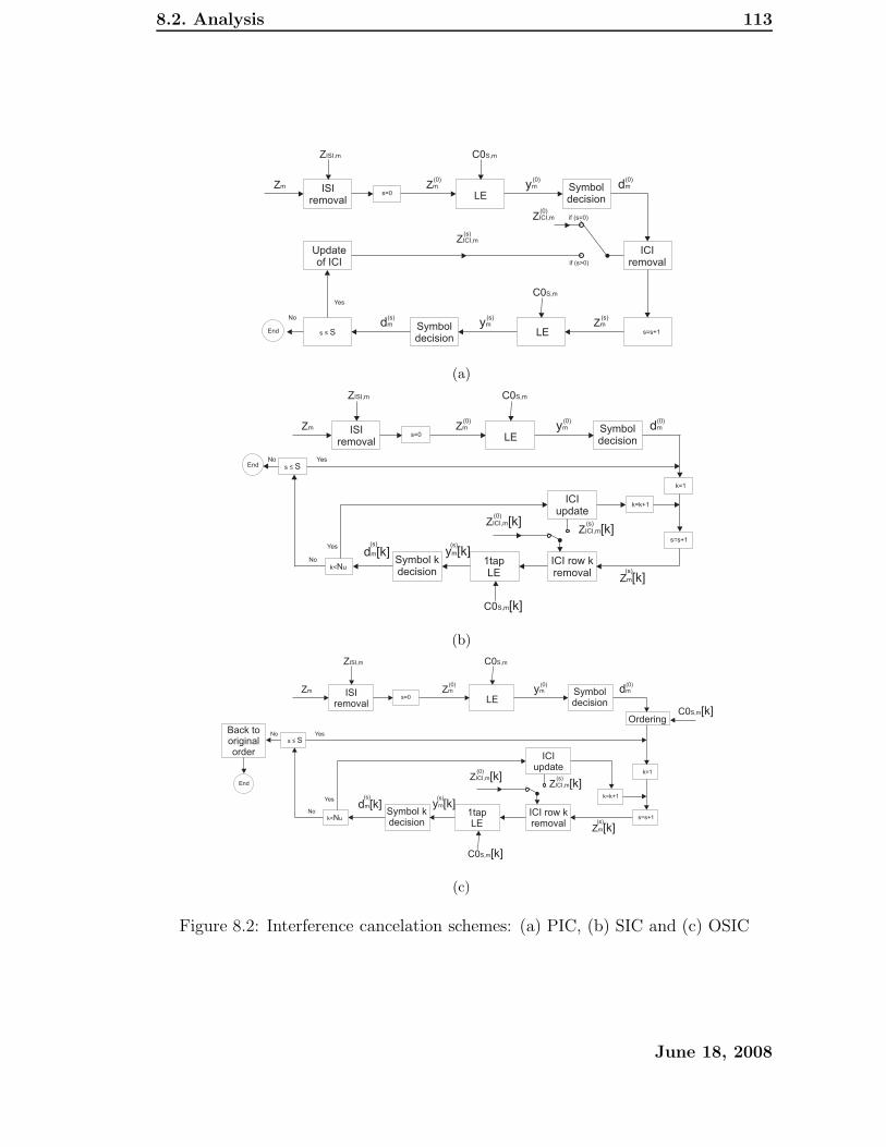
8.2. Analysis 113
ZICI,m(0)
ZICI,m(s)
Zm(s)
ym(s)
dm(s)
Yes
No
s ≤ SEnd
ICIremoval
Updateof ICI
Symboldecision
LE s=s+1
C0S,m
if (s=0)
if (s>0)
ZISI,m C0S,m
Zm ym(0)
dm(0)
ISIremoval LE
Symboldecision
s=0Zm
(0)
(a)
ZISI,m C0S,m
Zm ym(0)
dm(0)
End
ISIremoval LE
Symboldecision
k=k+1
k=1
s=s+1
ICI row kremoval
ICIupdate
s S≤
Yes
Yes
k< uN
No
No
s=0
1tapLE
Symbol kdecision
d [k]m
(s)
C0S,m[k]
y [k]m
(s)
Zm[k](s)
ZICI,m[k](0)
ZICI,m[k](s)
Zm(0)
(b)
k=k+1
k=1
s=s+1ICI row kremoval
ICIupdate
s ≤ SYes
Yes
k< uN
No
No 1tapLE
Symbol kdecision
d [k]m
(s)
C0S,m[k]
y [k]m
(s)
Zm[k](s)
ZICI,m[k](0)
ZICI,m[k](s)
OrderingC0S,m[k]
Back tooriginalorder
End
ZISI,m C0S,m
Zm ym(0)
dm(0)
ISIremoval LE
Symboldecision
s=0Zm
(0)
(c)
Figure 8.2: Interference cancelation schemes: (a) PIC, (b) SIC and (c) OSIC
June 18, 2008

8.2. Analysis 114
8.2.3 Performance analysis
In order to evaluate and compare the performance of the three proposed classical
IC schemes, a simulation scenario of Nfft = 512, Ts = 7, 68ns, QPSK modulation
scheme and a VehB PDP is proposed in figure 8.7. In a first step the effect of varying
the length of the CP on the uncoded BER when using a simple Linear Equalizer
(LE) is given on figure 8.3. As the CP length increases, the uncoded BER is lowered
until it achieves the theoretical bound where no interference is present (Tg > Tmed).
Figures 8.4, 8.5 and 8.7 correspond respectively to PIC, SIC and OSIC, where the
simulations are conducted with a very short CP of Tg = 0, 13µs. For all three
schemes there is a large BER gain already at S = 1. However even at S = 4 the
optimal performance isn’t achieved. In figure 8.8 the convergence rate of the three
classical schemes is studied. The difference between PIC, SIC and OSIC is that
OSIC has almost reached is optimal point after only S = 2, whereas PIC and SIC
need S = 4 iterations. Also the OSIC has a lower performance bound than PIC and
SIC.
All three schemes have the same initialization with the simple low complex LE.
This initialization could be improved with more advanced solutions such as ZF or
MMSE. Unfortunately such approaches are too computationally expensive . Another
way of improving the initial estimate would be to slightly increase the CP length up
to a reasonable value of 1µs or 2µs.
June 18, 2008
8.2. Analysis 115
5 10 15 20 25 30 35 40
10−4
10−3
10−2
10−1
100
Eb/N
o
BE
R
No Interference
LE, Tg = 0,13 µs
LE, Tg = 7,8 µs
LE, Tg = 15,6 µs
LE, Tg = 23,4 µs
Figure 8.3: LE
5 10 15 20 25 30 35 40
10−4
10−3
10−2
10−1
100
Eb/N
o
BE
R
No InterferencePIC S=1PIC S=2PIC S=3PIC S=4
LE, Tg = 0,13 µs
Figure 8.4: PIC
5 10 15 20 25 30 35 40
10−4
10−3
10−2
10−1
100
Eb/N
o
BE
R
OptimalSIC S=1SIC S=2SIC S=3SIC S=4
LE Tg = 0,13 µs
Figure 8.5: SIC
5 10 15 20 25 30 35 40
10−4
10−3
10−2
10−1
100
Eb/N
o
BE
R
No InterferenceOSIC S=1OSIC S=2OSIC S=3OSIC S=4
LE Tg = 0,13 µs
Figure 8.6: OSIC
Figure 8.7: Uncoded BER vs. Eb/No with Ts = 7, 68ns, Nu = Nfft = 512, VehB
June 18, 2008

8.3. The LCIC algorithm 116
1 2 3 4 510
−4
10−3
10−2
Iterations s
BE
R
PIC 26dBPIC 31dBSIC 26dBSIC 31dBOSIC 26dBOSIC 31dB
Figure 8.8: BER comparison of classical schemes for increasing iterations s
8.3 The LCIC algorithm
The OSIC scheme has the best performance of the three previously studied IC
cancelation schemes. However at each outer iteration s, N2u complex operations are
required to cancel the ICI as well as N2u complex operations are required at the
initialization to cancel the ISI. When looking closer at the correlation matrices C0m
and C1m in figure 8.13, where a 2D and 3D representation of log(arg(C0m[k′, k]))
and log(arg(C1m[k′, k])) give a snapshot example of the interference distribution
within the given matrices, {k′, k} ∈ [1, 128]2 and {k′, k} ∈ N2.
The figure can be interpreted as: strong interference comes from nearby subcarri-
ers, whereas distant subcarriers only interfere little the desired signal. The strongest
components are mostly to be found in the diagonal of C0m.
From these practical observations it would makes sense only to consider a limited
amount of subcarriers for IC, namely the ones with the strongest variance. By
choosing the Ith closest subcarriers the complexity can be reduced by a factor Nu
I.
The LCIC algorithms pseudo code is given in the following.
June 18, 2008
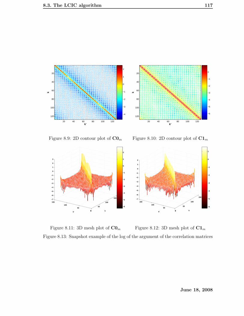
8.3. The LCIC algorithm 117
k’
k
20 40 60 80 100 120
20
40
60
80
100
120−4
−3
−2
−1
0
1
2
Figure 8.9: 2D contour plot of C0m
k’
k
20 40 60 80 100 120
20
40
60
80
100
120−6
−5
−4
−3
−2
−1
0
Figure 8.10: 2D contour plot of C1m
0
50
100
150
0
50
100
150
−7
−6
−5
−4
−3
−2
−1
0
1
2
3
kk’
−6
−5
−4
−3
−2
−1
0
1
2
Figure 8.11: 3D mesh plot of C0m
0
50
100
150
0
50
100
150
−7
−6
−5
−4
−3
−2
−1
0
1
2
kk’
−6
−5
−4
−3
−2
−1
0
1
Figure 8.12: 3D mesh plot of C1m
Figure 8.13: Snapshot example of the log of the argument of the correlation matrices
June 18, 2008

8.3. The LCIC algorithm 118
LCIC pseudo code:
Initialization phase :
s = 0
z(0)m = zm − C1band,m−1dm−1
y(0)m = C0−1
S,mz(0)m
d(0)m = csgn{y(0)
m }
Iterative phase :
Step1 : Matrix-Vector Ordering
Step2 : k = 1
Step3 : s = s+ 1
d(s)m = d(s−1)
m
Step4 : while(k ≤ Nu)
z(s)m [k] = z(s−1)
m [k] − C0band,m[k, (k − I, ..., k + I)]d(s)m [k − I, ..., k + I]
y(s)m [k] = C0−1
S,m[k, k]z(s)m [k]
d(s)m [k] = csgn{y(s)
m [k]}
k = k + 1
endwhile
Step5 : if(s ≤ S)goto Step2
else Reorder d(s)m and y(s)
m
endif
A graphical explanation of the initial ISI removal phase and a single iteration of ICI
canceling in Step 4 of the LCIC algorithm is given in figure 8.14. From this pseudo
code and figure the data flow of the LCIC unfolds naturally. When comparing this
targeted interference removal tot the graphical representation of C0m and C1m in
figure 8.13, the complexity reduction becomes straightforward.
The performance of the LCIC for varying initial estimate qualities is given in fig-
ure 8.15. Both sub-figures show that the the steepness of the uncoded BER curve is
highest for rather small values of I. Also the performance gain by increasing the CP
June 18, 2008

8.3. The LCIC algorithm 119
= - .
0
0
zm zm C1band,m-1 dm-1
(0)
I+1
I+1
(a)
= - .
0
0
zm zm C0band,m dm
(s)
I
I
(s)(s-1)
(b)
Figure 8.14: Matrix-vector illustration of two key steps in the LCIC algorithm: (a)
Initial one shot ISI removal, (b) Inner iteration k with ICI row removal
June 18, 2008
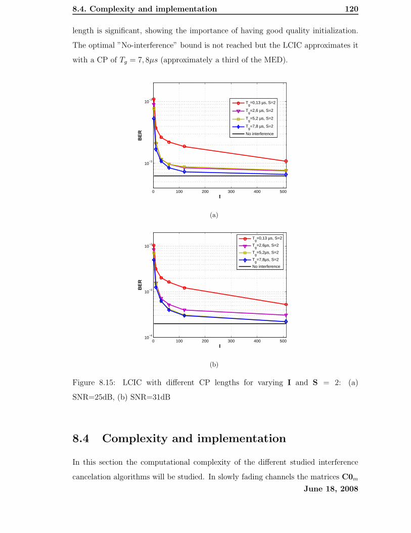
8.4. Complexity and implementation 120
length is significant, showing the importance of having good quality initialization.
The optimal ”No-interference” bound is not reached but the LCIC approximates it
with a CP of Tg = 7, 8µs (approximately a third of the MED).
0 100 200 300 400 500
10−3
10−2
I
BE
R
Tg=0,13 µs, S=2
Tg=2,6 µs, S=2
Tg=5,2 µs, S=2
Tg=7,8 µs, S=2
No interference
(a)
0 100 200 300 400 50010
−4
10−3
10−2
I
BE
R
Tg=0,13 µs, S=2
Tg=2,6µs, S=2
Tg=5,2µs, S=2
Tg=7,8µs, S=2
No interference
(b)
Figure 8.15: LCIC with different CP lengths for varying I and S = 2: (a)
SNR=25dB, (b) SNR=31dB
8.4 Complexity and implementation
In this section the computational complexity of the different studied interference
cancelation algorithms will be studied. In slowly fading channels the matrices C0m
June 18, 2008
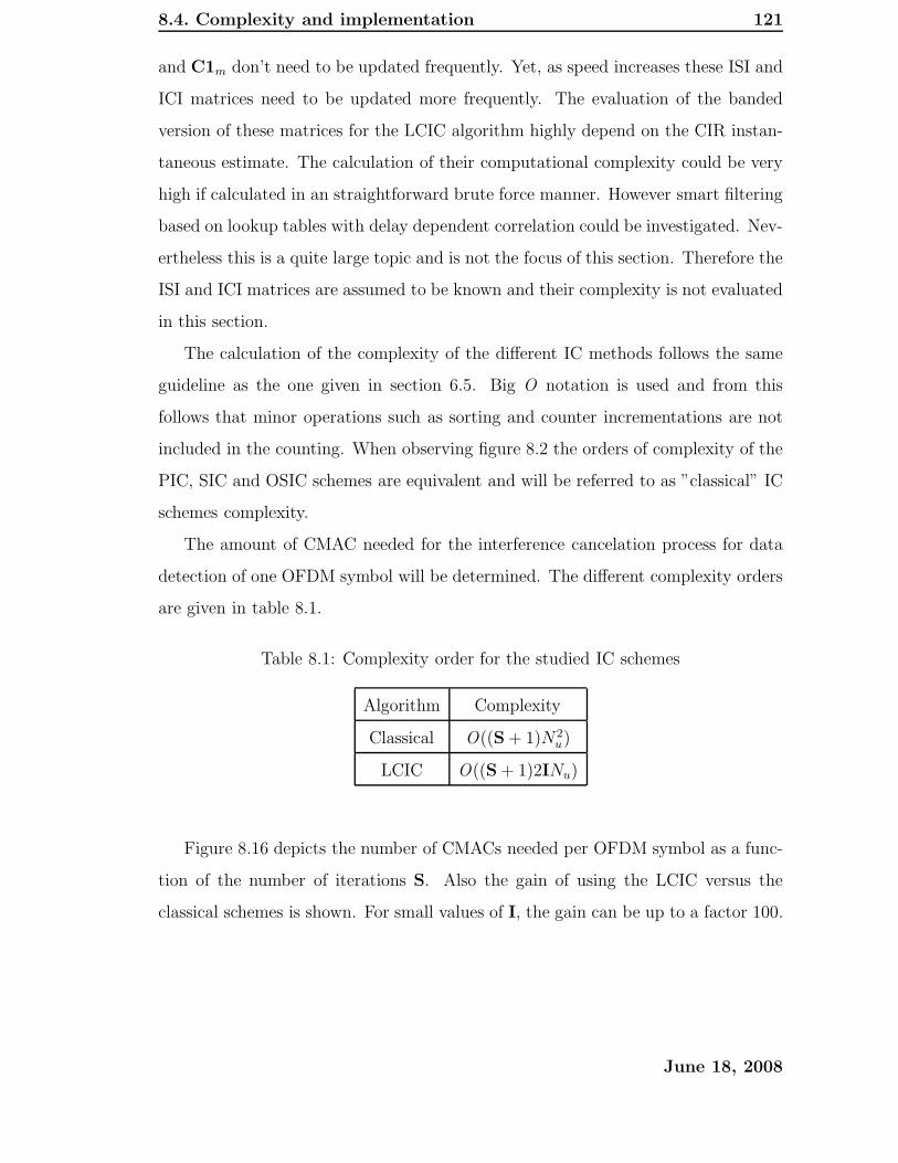
8.4. Complexity and implementation 121
and C1m don’t need to be updated frequently. Yet, as speed increases these ISI and
ICI matrices need to be updated more frequently. The evaluation of the banded
version of these matrices for the LCIC algorithm highly depend on the CIR instan-
taneous estimate. The calculation of their computational complexity could be very
high if calculated in an straightforward brute force manner. However smart filtering
based on lookup tables with delay dependent correlation could be investigated. Nev-
ertheless this is a quite large topic and is not the focus of this section. Therefore the
ISI and ICI matrices are assumed to be known and their complexity is not evaluated
in this section.
The calculation of the complexity of the different IC methods follows the same
guideline as the one given in section 6.5. Big O notation is used and from this
follows that minor operations such as sorting and counter incrementations are not
included in the counting. When observing figure 8.2 the orders of complexity of the
PIC, SIC and OSIC schemes are equivalent and will be referred to as ”classical” IC
schemes complexity.
The amount of CMAC needed for the interference cancelation process for data
detection of one OFDM symbol will be determined. The different complexity orders
are given in table 8.1.
Table 8.1: Complexity order for the studied IC schemes
Algorithm Complexity
Classical O((S + 1)N2u)
LCIC O((S + 1)2INu)
Figure 8.16 depicts the number of CMACs needed per OFDM symbol as a func-
tion of the number of iterations S. Also the gain of using the LCIC versus the
classical schemes is shown. For small values of I, the gain can be up to a factor 100.
June 18, 2008
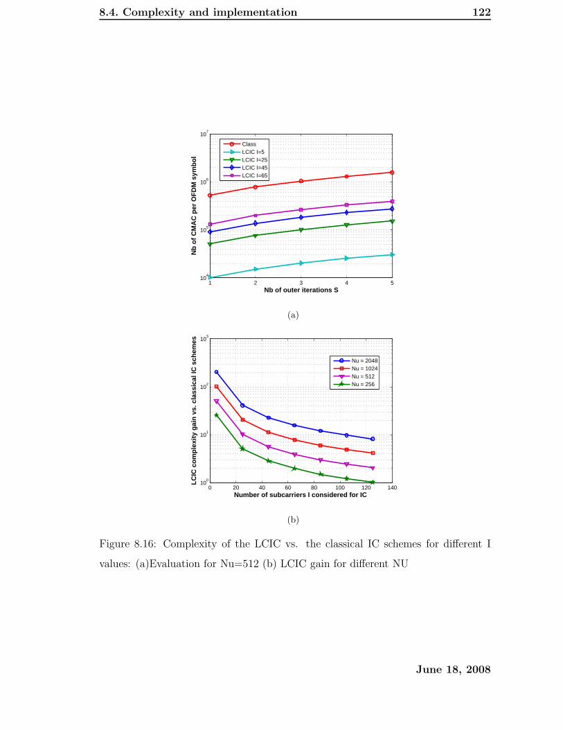
8.4. Complexity and implementation 122
1 2 3 4 510
4
105
106
107
Nb of outer iterations S
Nb
of C
MA
C p
er O
FD
M s
ymbo
l
ClassLCIC I=5LCIC I=25LCIC I=45LCIC I=65
(a)
0 20 40 60 80 100 120 14010
0
101
102
103
Number of subcarriers I considered for IC
LCIC
com
plex
ity g
ain
vs. c
lass
ical
IC s
chem
es
Nu = 2048Nu = 1024Nu = 512Nu = 256
(b)
Figure 8.16: Complexity of the LCIC vs. the classical IC schemes for different I
values: (a)Evaluation for Nu=512 (b) LCIC gain for different NU
June 18, 2008
8.5. Conclusion 123
8.5 Conclusion
In this chapter, it was shown how IC schemes could deal with short CP lengths.
Classical IC schemes were analyzed and led to the development of a novel reduced
complexity IC algorithm: the Low Complex Interference Cancelation scheme. The
use of the LCIC enables a considerable shortening of the CP length, and presents
itself as a tradeoff between affordable computational complexity and desired perfor-
mance.
Further investigations shall however be done before practical implementation
could be considered. Smarter evaluation of the ICI and ISI matrix bands is highly
relevant, as direct brute force computation would create a complexity bottleneck.
The interaction with channel estimation should also be investigated, more specifi-
cally an iterative joint channel estimation and IC would be of high relevance. The
estimation of the CIR tap phases, amplitudes and delays are a necessity to evaluate
C0m and C1m.
Finally, the developed analytical model of the received signal after the FFT has
been restricted to one single user using the full OFDM signal bandwidth. Yet, it
could be extended to a multiuser scenario using a similar approach as the LCIC. In
this case the algorithm would help in removing interference from an asynchronous
interferer and not from a to short CP. This could potentially be very beneficial,
increasing the frequency reuse of a system by lowering interference form other cells.
June 18, 2008

Chapter 9
Conclusions
9.1 Thesis summary
In this thesis a deep and careful study was carried out, based on mathematical anal-
ysis and simulations using Matlab, to understand the interaction between OFDM
parameter design and receiver algorithm choice.
This study was conducted in a physical layer, SISO OFDM, downlink LTE
generic frame structure context. As a result a CP length was proposed, two channel
estimation algorithms recommended for LTE UE receivers, a pilot scheme suggested
and a low complex interference cancelation algorithm developed.
The influence of CP length on SISO OFDM system capacity with LTE based
parameters was studied. The results showed that if only one CP length is to be
chosen, then a good tradeoff value would be in the range 4 to 5 µs. The received
SNR increased the sensitivity of the Capacity to the CP length. On the other hand,
higher other-cell interference will decrease the sensitivity to CP and its length could
be reduced. The useful OFDM symbol should be as long as the system design allows.
It was shown that the RMS delay spread of a PDP turns out not to be a sufficient
statistic to determine the optimal CP length as large variations of optimal CP length
can be observed for different PDPs having equal RMS delay spread. Thereby, the
whole PDP of the channel shall be considered when conducting CP design.
A framework has been provided for a choice of PACE frequency direction in-
terpolation algorithm in upcoming OFDM based standards. A classification has
124
9.1. Thesis summary 125
been carried out from a state of the art survey, showing that the linear solutions
provided in literature can be grouped into time and frequency domain approaches,
and categorized according to their a priori assumptions. A generalized estimator
formulation for linear PACE OFDM was derived, showing that each algorithm is
a particular case of this estimator and depends on the a priori channel informa-
tion taken into account. The effects of introducing virtual subcarriers as well as a
non-sample-spaced channel are studied and show that when Partial Bandwidth is
used, the TDLS and ML algorithms suffer from severe ill-conditioned matrices and
cannot be used as such if the number of virtual subcarriers is too large. From a com-
plexity point of view the FFT based algorithms showed their benefits compared to
RW, ENRA and WF. However the leakage effect due to non-sample-spaced channels
renders them unusable at higher SNRs than 10 dB. From the studied algorithms,
only the RW, ENRA an WF are robust to this leakage effect. We conclude that
the WF and ENRA are the most suitable algorithms from both performance and
complexity point of view as long as accurate CIR delays are provided. The accuracy
and complexity of this methods depend on richness and the variability over time
of the delay subspace. In practice it is therefore not trivial to determine the best
solution. The RWF will work in all cases, within the assumptions and gives a fixed
degradation from known channel performance, depending on the MED of the CIR.
The ENRA/WF solutions will be able to perform up to 1-2 dB better than this
depending on the channel scenario but their reliability is determined by the CIR
delay estimate accuracy. Therefore, in a first release of LTE, the RWF solution with
low rank precalculated filter is recommended. If better performance is needed, the
ENRA should then be considered with optimized delay tracking. The WF is not
that interesting, as the ENRA gives almost same performance without having to
track the different CIR tap powers.
A suitable pilot distribution for downlink LTE has been proposed by simulation
approach taking into considerations the practical constraints that this implies. First
the robustness of different interpolation algorithms against variation of pilot spacing
was investigated. In the frequency direction the RWF and LI turned to be very
sensitive to minor changes in pilot spacing in the case of CIR with long delays.
June 18, 2008

9.2. Future work 126
When the CIR delays are short, sensitivity to varying frequency direction pilots
spacing is quasi-insignificant. The ENRA and WF using a priori knowledge of
tap delay location, turned to be very robust to pilot spacing variation even in the
case of large CIR delays. In the time direction the importance of algorithm choice
is little relevant in the low speed scenario as the channel is quasi-static over the
duration of one time slot. The overall importance of time direction interpolation is
however reduced as ICI is irreducible when using a classical OFDM1 tap equalizer.
Also DRX-DTX, and latency requirements force the estimation to be done within
the duration of one time slot estimation, and inter-slot interpolation is undesirable.
One fixed pilot pattern is proposed for downlink LTE from the derived method. The
pilot scheme will have an overhead of 3,6%, cover all considered channel scenarios
and will have support for high mobile speeds up to 300kmph. Spectral efficiency
results are shown for a wide range of proposed modulation and coding schemes going
from -10 dB to 40 dB SNR, and confirm the validity of the proposed distribution.
Finally, it was shown how IC schemes could deal with scenarios where the CIR
tap delays are longer than the CP length. Classical IC schemes were analyzed
and led to the development of a novel reduced complexity IC algorithm: the LCIC
scheme. The use of the LCIC enables a considerable shortening of the CP length,
and presents itself as a tradeoff between affordable computational complexity and
desired performance.
9.2 Future work
Regarding PACE, future perspectives would be to investigate the feasibility of fre-
quency direction interpolation algorithm using a priori tap delay knowledge such as
ENRA, thereby enhancing the BLER performance and allowing lower pilot overhead
than in current PSAM OFDM systems. More specifically low complex and accurate
tap delay tracking in UE terminals would be the key for this to be done. The scenario
of single frequency network MBMS transmitting continuous data would increase the
importance of time averaging, filtering and predictive algorithms. Adaptive PACE
algorithms in UE terminals supporting both one shot estimators and averaging esti-
June 18, 2008
9.2. Future work 127
mators should be investigated. The correlation properties in MIMO channels should
be used for further improvements of channel estimation accuracy and complexity re-
duction.
Regarding the LCIC algorithm, further investigations shall be done before prac-
tical implementation could be considered. Smart computation and estimation of the
ICI and ISI matrix bands is highly relevant, as direct brute force computation would
create a complexity bottleneck. The interaction with channel estimation should also
be elaborated, more specifically an iterative joint channel estimation and IC would
be of high relevance. The estimation of the CIR tap phases, amplitudes and delays
are a necessity to evaluate C0m and C1m. The developed analytical model of the
received signal after the FFT has been restricted to one single user using the full
OFDM signal bandwidth. Yet, it could be extended to a multiuser scenario using
a similar approach as the LCIC. In this case the algorithm would help in removing
interference from an asynchronous interferer and not from a to short CP. This could
potentially be very beneficial, increasing the frequency reuse of a system by lowering
interference form other cells.
As a final comment to this thesis, one is lead to observe following. Standardiza-
tion of future mobile wireless systems will most likely continue to have requirements
on increasing spectral efficiency and in the same time on limiting terminal compu-
tational complexity and power consumption. These requirements work against each
other and even though technical solutions exist for increasing the spectral efficiency,
these can’t be to expensive. Thereby one can state that solutions to increase system
spectral efficiency must be cheap from a computational complexity and the related
power consumption.
June 18, 2008

Bibliography
[1] 3GPP TR 25.814 V2.0.0 (2006), ”Physical Layer Aspects for evolved Universal
Terrestrial Radio Access (UTRA)”
[2] 3GPP TR 25.913 V7.3.0 (2006-03), ”Requirements for Evolved UTRA (E-
UTRA) and Evolved UTRAN (E-UTRAN)”
[3] 3GPP TR 25.892 V6.0.0 (2004). ”Feasability Study for Orthogonal Frequency
Division Multiplexing (OFDM) for UTRAN enhancement”
[4] 3GPP TS 36.201 V0.2.0 (2006-11), ”Technical Specification Group Radio Access
Network; LTE Physical Layer - General Description (Release 8)”
[5] 3GPP TS 36.211 V1.1.0 (2007-05), ”Technical Specification Group Radio Access
Network; Physical Channels and Modulation (Release 8)”
[6] 3GPP TS 36.212 V0.2.1 (2006-11), ”Technical Specification Group Radio Access
Network; Multiplexing and channel coding (Release 8)”
[7] 3GPP TSG RAN WG1 Meeting 41 R1-050386 (May 2005), ”Views on OFDM
Parameter Set for Evolved UTRA Downlink”
[8] ANSI/IEEE Std 802.11, 1999 Edition (R2003) Information technology - Telecom-
munications and information exchange between systems - Local and metropolitan
area networks - Specific requirements. Part 11: Wireless LAN Medium Access
Control (MAC) and Physical Layer (PHY) Specifications
[9] IEEE Std 802.11a-1999(R2003) Supplement to IEEE Standard for Information
technology - Telecommunications and information exchange between systems -
128
Bibliography 129
Local and metropolitan area networks - Specific requirements. Part 11: Wireless
LAN Medium Access Control (MAC) and Physical Layer (PHY) Specifications.
High-speed Physical Layer in the 5 GHz band.
[10] IEEE Std 802.11gTM -R2003 IEEE Standard for Information technology -
Telecommunications and information exchange between systems - Local and
metropolitan area networks - Specific requirements. Part 11: Wireless LAN
Medium Access Control (MAC) and Physical Layer (PHY) Specifications. Fur-
ther Higher Data Rate Extension in the 2.4 GHz band.
[11] Final draft ETSI EN 300 401 v1.4.1 (2006-01) Radio Broadcasting Systems;
Digital Audio Broadcasting (DAB) to mobile, protable and fixed receivers.
[12] ETSI EN 300 744 V1.5.1 (2004-11) Digital Video Broadcasting (DVB);Framing
structure, channel coding and modulation for digital terrestrial television
[13] ETSI EN 302 304 V1.1.1 (2004-11) Digital Video Broadcasting
(DVB);Transmission System for Handheld Terminals (DVB-H)
[14] IEEE Std 802.16-2004 (Revision of IEEE Std 802.16-2001) IEEE Standard for
Local and Metropolitan Area Networks Part 16: Air Interface for Fixed Broad-
band Wireless Access Systems
[15] 802.16e-2005 and IEEE Std 802.16-2004/Cor1-2005 IEEE Standard for Local
and metropolitan area networks Part 16: Air Interface for Fixed and Mobile
Broadband Wireless Access Systems Amendment 2: Physical and Medium Ac-
cess Control Layers for Combined Fixed and Mobile Operation in Licensed Bands
and Corrigendum 1
[16] Recommendation ITU-R M.1225, ”Guidelines for evaluation of radio transmis-
sion technologies for IMT-2000,” 1997
[17] G. E. Moore, ”Cramming more components onto integrated circuits” McGraw-
Hill, Electronics Magazine, Volume 38, Number 8, April 19, 1965
[18] R.W. Chang , Synthesis of Band-Limited Orthogonal Signals for Multichannel
Data Transmission, Bell System Technical Journal, 45, pp. 1775-1796, 1966
June 18, 2008

Bibliography 130
[19] L.J. Cimini, Analysis and Simulation of a Digital Mobile Channel Using Or-
thogonal Frequency-Division Multiplexing, IEEE Transactions on Communica-
tions, 33, 7, pp. 665-675, 1985
[20] J. A. C. Bingham, ”Multicarrier Modulation for Data Transmission: An Idea
Whose Time Has Come,” IEEE Commun. Mag. vol. 31, pp 5-14, May 1990.
[21] C. Rom, T.B. Sørensen, P.E. Mogensen and B. Vejlgaard, ”Impact of Cyclic
Prefix length on OFDM system Capacity”, Proceedings of the WPMC’05 Vol.3,
pp. 1871-1875, 18-22 September 2005
[22] H. Steendam, M. Moenclaey, ”Analysis and Optimization of the Performance of
OFDM on Frequency-Selective Time-Selective Fading Channels,” IEEE Trans.
Commun. vol. 47, pp. 1811-1819, dec. 1999
[23] J. Li, M. Kavehrad, Effect of Time Selective Multipath Fading on OFDM
Systems for Broadband Mobile Applications, IEEE Com. Letters, vol. 3, no. 12,
Dec. 1999.
[24] M. Russel, G. L. Stuber, Interchannel Interference Analysis of OFDM in a
Mobile Environment, Proc. VTC 95, p. 820, 1995.
[25] S.R. Searle, Matrix Algebra Useful for Statistics. New York: Wiley, 1982.
[26] L. Hanzo, M. Mnster, B. J. Choi, T. Keller, OFDM and MC-CDMA for
Broadband Multi-User Communications, WLANs and Broadcasting, Wiley, 2003
[27] R. Van Nee, R. Prasad, OFDM for Wireless Multimedia Communications,
Artech House, 2000
[28] A. R. S. Bahai, B. R. Saltzberg, M. Ergen, Multi-Carrier Digital Communi-
cations Theory and Applications of OFDM, Second Edition, Springer, 2004
[29] A. V. Oppenheim and R. W. Schafer, Discrete-Time Signal Processing (2nd
Edition), Prentice Hall, 1999, ISBN-13: 978-0-137-54920-7
[30] J. D. Parsons, The mobile radio propagation channel (2nd Edition), Wiley,
2000, ISBN-13: 978-0-471-98857-1
June 18, 2008

Bibliography 131
[31] J. Proakis, Digital Communications (4th edition), Mc Graw Hill, 2001, ISBN-
10: 0072321113
[32] T. Moon, W. Stirling, ”Mathematical Mehtods and Algorithms for Signal
Processing”. Prentice Hall, 2000
[33] Thomas H. Cormen, Charles E. Leiserson, Ronald L. Rivest, and Clifford Stein,
”Introduction to Algorithms”. Second Edition, MIT Press and McGraw-Hill,
2001. ISBN 0-262-03293-7
[34] Harold Jeffreys and Bertha Jeffreys, ” Methods of Mathematical Physics
(Third Edition)” Cambridge University Press, 1999, ISBN: 0521664020
[35] J. Harold. Ahlberg, ”The Theory of Splines and Their Applications ”, Academic
Pr (June 1967), ISBN: 0120447509
[36] Sergio Verdu, ”Multiuser detection”, Cambridge University Press, 1998, ISBN
0-521-59373-5
[37] Na Wei, ”MIMO Techniques in UTRA Long Term Evolution”, Ph.D. thesis,
Department of Electronic Systems, Aalborg University, Denmark, June 2007.
[38] D. Coppersmith and S. Winograd. ”Matrix multiplication via arithmetic pro-
gressions.” In Proc. Nineteenth ACM Symp. Theory of Computing, pages 1-6,
1987
[39] Kaare Brandt Pedersen and Michael Syskind Pedersen, ”The Matrix Cook-
book.” Version: Fbruary 16, 2006
[40] Max Welling, ”The Kalman Filter,” Lecture Note.
[41] 3GPP TR 25.848, Physical Layer Aspects of UTRA High Speed Downlink
Packet Access.
[42] S. M. Alamouti, ”A simple transmit diversity technique for wireless communi-
cation” IEEE Journal on Selected Areas in Communications, Volume 16, Issue
8, Oct. 1998 Page(s):1451 - 1458
June 18, 2008
Bibliography 132
[43] G. J. Foschini, ”Layered Space-Time Architecture for Wireless Communication
in a Fading Environment When Using Multiple Antennas” Bell Labs Technical
Journal, Vol. 1, No. 2, Autumn 1996, pp 41-59.
[44] C. Rom, C. N. Manchon, T.B. Sørensen, P.E. Mogensen and Luc Deneire,
”Analysis of Time and Frequency Domain PACE Algorithms for OFDM with
Virtual Subcarriers” Personal, Indoor and Mobile Radio Communications, 2007
IEEE 18th International Symposium Sept. 2007 Pages: 1-5
[45] L. Schumacher, J. P. Kermoal, F. Frederiksen, K. I. Pedersen, A. Algans and
P. E. Mogensen, MIMO Channel Characterisation, IST Project IST- 1999-11729
METRA Deliverable 2, February 2001.
[46] 3GPP TR 25.943, Deployment aspects.
[47] 3GPP TS 36.300, v8.2.0 (2007-09), ”E-UTRA and E-UTRAN Overall descrtip-
tion, stage2”
[48] H. Holma and A. Toskala, Eds., WCDMA for UMTS, Radio Access For Third
Generation Mobile Communications, Wiley, Chichester, UK, second edition,
2002.
[49] T. E. Kolding, F. Frederiksen, P. E. Mogensen, Performance aspects of
WCDMA systems with High Speed Downlink Packet Access (HSDPA), VTC
Fall, July, 2002.
[50] P. O. Vidal, ”Analysis of OFDM for UTRAN enhancement,” Master thesis for
Aalborg University, Institute of Electronic Systems, Departement of Communi-
cation Technology, Cellular Systems.
[51] G. Monghal and Y. Malidor, ”PSAM-Based Channel Estimation applied on a
novel OFDM Downlink Equalization technique”, Master thesis for Aalborg Uni-
versity, Institute of Electronic Systems, Departement of Communication Tech-
nology, Cellular Systems, June 2005
June 18, 2008
Bibliography 133
[52] C. N. Manchon, ”Next Generation of Mobile Systems: The Channel Estimation
Problematic in Downlink OFDM”, Master Thesis, Department of Communica-
tion Technology, Aalborg University, May 15, 2006
[53] H. Yaghoobi, ”Scalable OFDMA Physical Layer in IEEE 802.16 Wireless
MAN,” Intel Technology Journal, Volume8, Issue3, 2004
[54] F. Tufvesson, T. Maeseng ”Optimization of Sub-Channel Bandwidth for mo-
bile OFDM systems,” MMT’97, Melbourne, Australia, dec. 1997
[55] J. L. Seoane, S. K. Wilson, S. Gelfand, ”Analysis of Intertone and Interblock
Interference in OFDM when the length of the Cyclic Prefix is shorter than the
length of the Channel Impulse Response,” Globecom 97, Pheonix Arizona, Nov
1997.
[56] M. Batariere, K. Braum, T. P. Krauss ”Cyclic Prefix Length Analysis for 4G
OFDM Systems,” VTC’04, Los Angeles, USA, sept. 2004
[57] C. Lim, Y. Chang, J. Cho, P. Joo, H. Lee, ”Novel OFDM Transmission
Scheme to Overcome ISI Caused by Multipath Delay Longer than Cyclic Prefix,”
VTC’05, Stockholm, Sweeden, May. 2005.
[58] K. L. Baum, T. A. Kostas, P. J. Sartori, B. K. Classon, ”Performance Charac-
teristics of Cellular Systems with Different Link Adaptation Strategies,” IEEE
Trans. Vehicular Technology, Vol. 52, No. 6, November 2003.
[59] L.J. Cimini, Jr., Analysis and Simulation of a Digital Mobile Channel Using Or-
thogonal Frequency-Division Multiplexing. IEEE Trans. Commun., vol.33, no.7,
pp. 665-675, July 1985.
[60] R. Gonzlez and F. Bader ”Time-Frequency Spacing Design for PACE in OFDM
Systems,” IST 14th Summit, Dresden 19-23 June 2005
[61] S. Coleri, M. Ergen, A. Puri and A. Bahai, ”Channel estimation techniques
based on pilot arrangement in OFDM systems,” IEEE Trans. Broadcasting, vol
48, pp. 223-229, Sept. 2002.
June 18, 2008
Bibliography 134
[62] K. F. Lee and D. B. Williams, ”Pilot-symbol-assisted channel estimation for
space-time coded OFDM systmes,” EURASIP J. Applied Signal Process., vol. 5,
pp. 507-516, May 2002.
[63] P. Hoeher,S. Kaiser and I. Robertson, ”Two-dimensional pilot-symbol-aided
channel estimation by wiener filtering,” in Proc. Int. Conf. Acoustics Speech and
Signal Processing (ICASSP), 1997, pp. 1845-1848.
[64] P. Hoeher, S. Kaiser and I. Robertson, ”Pilot-symbol-aided channel estimation
in time and frequency”, in Proc. Sixth Communication Theory Mini-Conference
in conjunction with IEEE GLOBECOM 97, Phoenix, Arizona, pp. 90-96, Novem-
ber 1997
[65] P. Hoeher, ”TCM on frquency-selective land-mobile fading channels,” in Inter-
national Workshop on Digital Communications, (Tirrenia, Italy), pp. 317-328,
September 1991.
[66] J.-J. van de Beek,O. Edfors, M. Sandell, S. K. Wilson and P.O. Borjesson ”On
channel estimation in OFDM systems,” in Proc. IEEE VTC’96,, Nov. 1996, pp.
815-819.
[67] O. Edfors, M. Sandell, J. van de Beek, S. K. Wilson, and P. O. Borjesson,
”OFDM channel estimation by singular value decomposition,” in Proceedings
of Vehicular Technology Conference, vol. 2, (Atlanta, GA USA) pp. 923-927,
April-May 1996
[68] O. Edfors, M. Sandell, J. van de Beek, S. K. Wilson, and P. O. Borjesson,
”OFDM channel estimation by singular value decomposition,” in IEEE Trans.
Commun., vol. 46, pp. 931-939, July 1998
[69] Igor A. Tolochko, ”Channel estimation for OFDM systems with transmitter
diversity”, Doctor of Philosophy, Centre for Telecommunications and Micro-
Electronics, Victoria University of Technology, August 2005
June 18, 2008
Bibliography 135
[70] O. Simeone, Y. Bar-Ness, U. Spagnolini, ”Pilot-Based Channel Estimation
for OFDM Systems by Tracking the Delay-Subspace” in IEEE Trans. Wireless.
Comm., vol. 3, no. 1, jan 2004
[71] R. Negi and J. Cioffi, ”Pilot tone Selection for channel estimation in a mobile
OFDM system,” in IEEE Trans. Consumer Electron., vol. 44, pp. 1122-1128.
[72] L. Deneire, P. Vandenameele, L. van der Pierre, B. Gyselinckx, and M. Engels
”A low Complexity ML channel estimator for OFDM,” in IEEE Trans. Commun,
vol. 51, no.2, pp 135-140, February 2003.
[73] H. Schmidt, V. Khn, K.D. Kammeyer, R. Rueckriem, and S. Fechtel,
”Channel tracking in wireless OFDM systems,” in SCI 2001, Orlando, Florida,
USA, 22-25 July 2001.
[74] M.H. Hsieh and C.H. Wei, ”Channel estimation for OFDM systems based
on comb-type pilot arrangement in frequency selective fading channels,” IEEE
Trans. Consumer Electronics, vol.44, pp. 217-225, Feb. 1998.
[75] B. Yang, K.B. Letaief, R.S. Cheng and Z. Cao, ”Channel estimation for OFDM
transmission in multipath fading channels based on parameteric channel mod-
elling,” in IEEE Trans. Commun., vol. 49, pp. 467-479, March 2001.
[76] D. Schafhuber, G. Matz and F. Hlawatsch ”Adaptive Wiener Filters for
Time-Varying Channel Estimation in OFDM Systems” 2003 IEEE International
Conference on Acoustics, Speech, and Signal Processing, (ICASSP ’03), vol.4,
pp. 688-91, 6-10 April 2003
[77] G. Auer, S. Sand and A. Dammann, ”Comparison of Low Complexity OFDM
Channel Estimation Techniques” In Proc. of Int OFDM Workshop, Hamburg,
Germany, September 2003
[78] Y. Li, L. J. Cimini, and N. R. Sollenberger, ”Robust channel estimation for
OFDM systems with rapid dispersive fading,” in IEEE Trans. Commun., vol.
46, pp. 902-915, July 1998
June 18, 2008
Bibliography 136
[79] M. Morelli and U. Mengali, ”A Comparison of Pilot-Aided Channel Estimation
Methods for OFDM Systems,” in IEEE Trans. Signal Proc., vol. 49, pp. 3065-
3073, December 2001
[80] F. Tufvesson, M. Faulkner, and T. Maseng, ”Pre-Compensation for Rayleigh
Fading Channels in Time Divisoin Duplex OFDM Systems,” in Proceedings of
6th International Workshop on Intelligent Signal Processing and Communication
Systems, (Melbourne, Australia), pp. 57-33, IEEE, November 5-6 1998.
[81] A. Tikhonov and V. Arsenin, Solutions of Ill-Posed Problems. Washington:
Winston, 1977.
[82] M.J. Frenandez-Getino Garcia, S. Zazo and J.M. Paez-Borrallo, ”Pilot pat-
terns for channel estimation in OFDM” Electronic Letters, Vol.36, No.12 ,pp.
1049-1050, 8th of June 2000
[83] W. Zhang, X.G. Xia, P.C. Ching and W.K. Ma, ”On the number of pilots
for OFDM system in multipath fading channels” ICASSP 2004, Volume 4, 17-21
May 2004 Page(s):iv-381 - iv-384
[84] J.W. Choi and Y.H. Lee, ”Desing of the Optimum Pilot Pattern for Channel
Estimation in OFDM Systems,” Global Telecommunications Conference, 2004,
GLOBECOM04, pp. 3661- 3665 Vol.6, IEEE, 29 Nov.-3 Dec. 2004.
[85] H. Nyquist, ”Certain topics in telegraph transmission theory”, Trans. AIEE,
vol. 47, pp. 617-644, Apr. 1928
[86] E. Al-Susa and R. Ormondroyd ”A Predictor-Based Decision Feedback
Channel Estimation Method for COFDM with High Resilience to Rapid Time-
Variations,” in Proceedings of Vehicular Conference, vol. 1, (Amsterdam, Nether-
lands), pp. 273-278, IEEE, September 19-22 1999
[87] A. Stamoulis, S.N. Diggavi, N. Al-Dhahir, ”Intercarrier interference in MIMO
OFDM”, in IEEE Transactions, vol. 50, issue 10, pp 2451-2464 Oct. 2002
[88] P. Schniter, ”Low-Complexity Equalization of OFDM in Doubly Selective
Channels”, IEEE Trans. On Signal Processing, Vol. 52, No. 4, apr. 2004
June 18, 2008

Bibliography 137
[89] T. V. Sreenivas adn P. V. S. Rao, ”High-Resolution Narrow-Band Spectra by
FFT Prunning,” in IEEE Trans. on Acoustics Speech and Signal Processing, vol.
assp-28, pp. 254-257, No.2, April 1980
[90] B. Lu and X. Wang, ”Bayesian Blind Turbo Reciever for Coded OFDM
Systems with Frequency Offset and Frequency-Selective Fading,” IEEE Journal
on Selected Areas in Communications, vol. 19, pp. 2516-2527, December 2001.
[91] Chengyang Li and Sumit Roy, ”Subspace-Based Blind Channel Estimation
for OFDM by Explointing Virtual Carriers,” in IEEE Trans. Commun., vol. 2,
pp. 141-150, Jan 2003
[92] Marc C. Necker and Gordon L. Stuber ”Totally Blind Channel Estimation
for OFDM on Fast Varying Mobile Radio Channels” in IEEE Trans. Commun.,
vol. 3, pp. 1514-1524
[93] M Munster and L. Hanzo ”Second-order channel parameter estimation assisted
cancellation of channel variation-induced inter-subcarrier interference in OFDM
systems,” EURCON 2001, Volume 1, 4-7 July 2001 Page(s):1 - 5
[94] A. J. Jerri. ”The Shannon sampling theoremIts various extensions and appli-
cations: A tutorial review” Proceedings of the IEEE, Volume 65, Issue 11, Nov.
1977 Page(s):1565 - 1596
[95] N. Wei, A. Pokhariyal, C. Rom, B.E. Priyanto, F. Frederiksen, C. Rosa, T.
B. Srensen, T. Kolding, P.E. Mogensen, ”Baseline E-UTRA Spectral Efficiency
Evaluation,” IEEE Vehic. Technol. Conf., Montreal, Canada, October 2006
[96] ”Matlab, The Language of Technical Computing”, version 7.0.4.365 (R14), Ser-
vice Pack 2. Copyright 1984-2005, the Mathworks, Inc.
[97] D. Kim, G. L. Stuber, Residual ISI Canccllation for OFDM with Application
to HDTV Broadcasting, IEEE J. Select. Areas in Conim., vol. 16, no. 8, Oct.
1998.
June 18, 2008
Bibliography 138
[98] C. Lim, Y. Chang, J. Cho, P. Joo, H. Lee, Novel OFDM Transmission
Scheme to Overcome ISI Caused by Multipath Delay Longer than Cyclic Prefix,
VTC05, Stockholm, Sweeden, May. 2005
[99] P. J. W. Melsa, R. C. Younce, C. E. Rohrs, ”Impulse response shortening
for discrete multitone transceivers,” IEEE Trans. Commun., vol. 44, no.12, pp.
1662-1672, Dec. 1996.
[100] R. Schur, Impulse Compression for OFDM Transmission over Time-Varying
Multipath Channels, Proc. IEEE VTC 2002-fall, vol.2, pp.1074-1076, September
2002.
[101] N. Suzuki, H. Uehara, M. Yokoyama, A New OFDM Demodulation Method
with Variable Length Effective Symbol and ICI Canceller., IEICE Trans Funda-
mentals, vol.E85-A, no.12, December 2002.
[102] N. Suzuki, T. Shibata, N. Itoh and M. Yokoyama, ”OFDM demodulation
method with variable effective symbol duration”,IEICE Trans. Fundamentals,
vol. E85-A, no.7, pp. 1665-1674, July 2002.
[103] Y. C. Yoon, R Kohno and H. Imai, ”A spread-spectrum multiacces system
with cochannel interference cancellation for mulitpath fading channels”, IEEE
Journal Sel. Areas Commun., vol.11, no.7, pp.1067-1075, Sep. 1993
[104] R4-071135, Agreed LTE UE demodulation performance simulation assump-
tions, Motorola
[105] R4-071297 LTE UE demodulation results, Ericsson
[106] R4-071325 Ideal simulations results for E-UTRA PDSCH with Rel-7 coding
chain, NEC
June 18, 2008
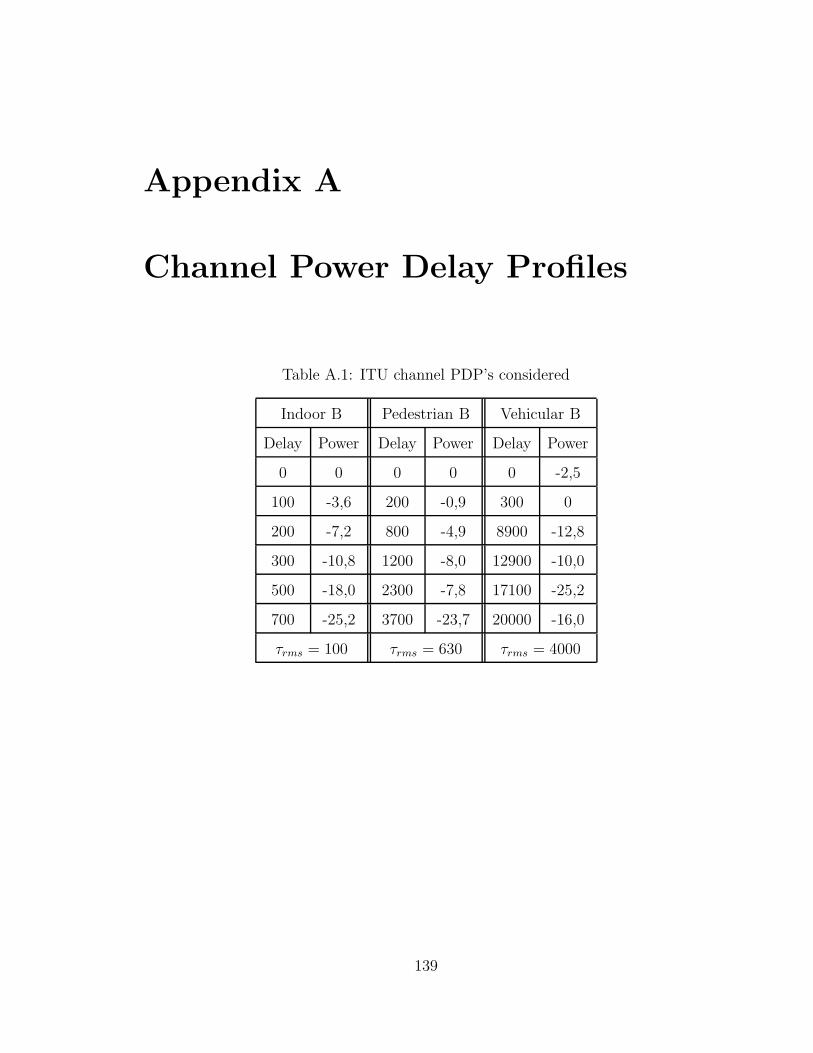
Appendix A
Channel Power Delay Profiles
Table A.1: ITU channel PDP’s considered
Indoor B Pedestrian B Vehicular B
Delay Power Delay Power Delay Power
0 0 0 0 0 -2,5
100 -3,6 200 -0,9 300 0
200 -7,2 800 -4,9 8900 -12,8
300 -10,8 1200 -8,0 12900 -10,0
500 -18,0 2300 -7,8 17100 -25,2
700 -25,2 3700 -23,7 20000 -16,0
τrms = 100 τrms = 630 τrms = 4000
139
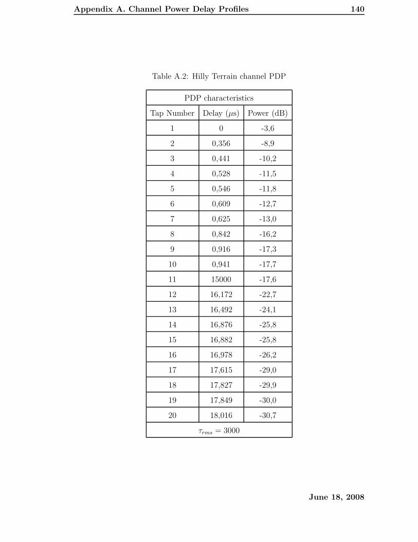
Appendix A. Channel Power Delay Profiles 140
Table A.2: Hilly Terrain channel PDP
PDP characteristics
Tap Number Delay (µs) Power (dB)
1 0 -3,6
2 0,356 -8,9
3 0,441 -10,2
4 0,528 -11,5
5 0,546 -11,8
6 0,609 -12,7
7 0,625 -13,0
8 0,842 -16,2
9 0,916 -17,3
10 0,941 -17,7
11 15000 -17,6
12 16,172 -22,7
13 16,492 -24,1
14 16,876 -25,8
15 16,882 -25,8
16 16,978 -26,2
17 17,615 -29,0
18 17,827 -29,9
19 17,849 -30,0
20 18,016 -30,7
τrms = 3000
June 18, 2008
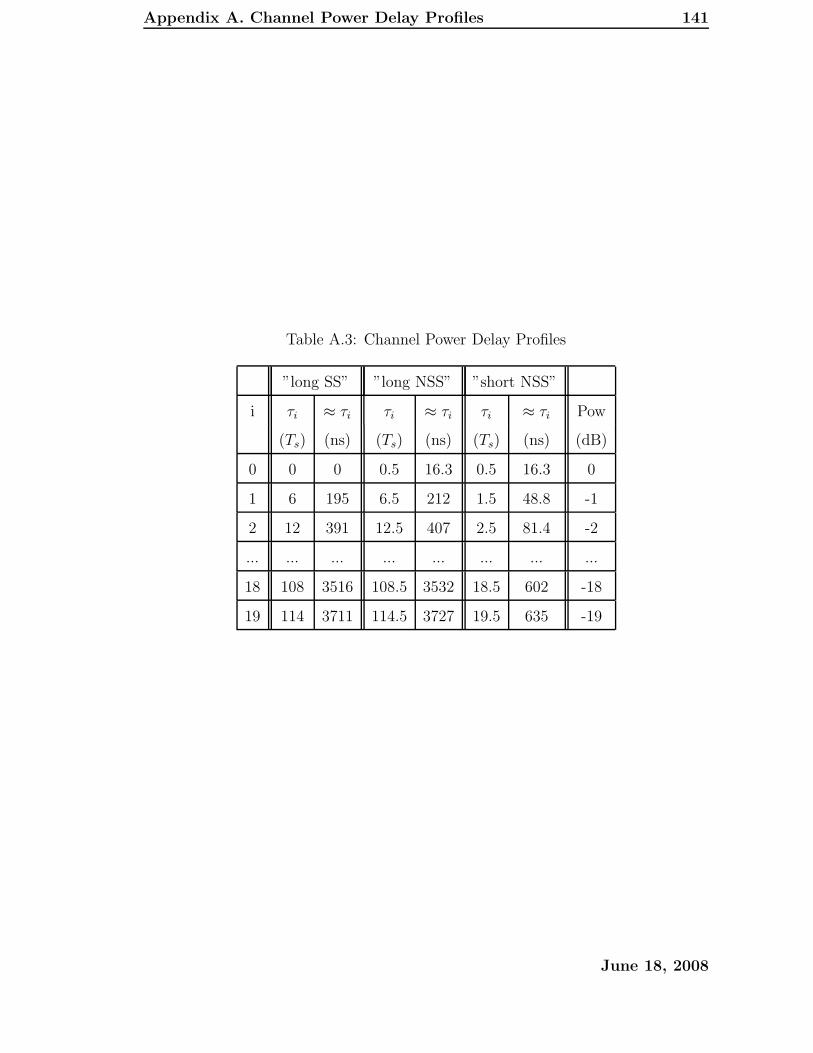
Appendix A. Channel Power Delay Profiles 141
Table A.3: Channel Power Delay Profiles
”long SS” ”long NSS” ”short NSS”
i τi ≈ τi τi ≈ τi τi ≈ τi Pow
(Ts) (ns) (Ts) (ns) (Ts) (ns) (dB)
0 0 0 0.5 16.3 0.5 16.3 0
1 6 195 6.5 212 1.5 48.8 -1
2 12 391 12.5 407 2.5 81.4 -2
... ... ... ... ... ... ... ...
18 108 3516 108.5 3532 18.5 602 -18
19 114 3711 114.5 3727 19.5 635 -19
June 18, 2008
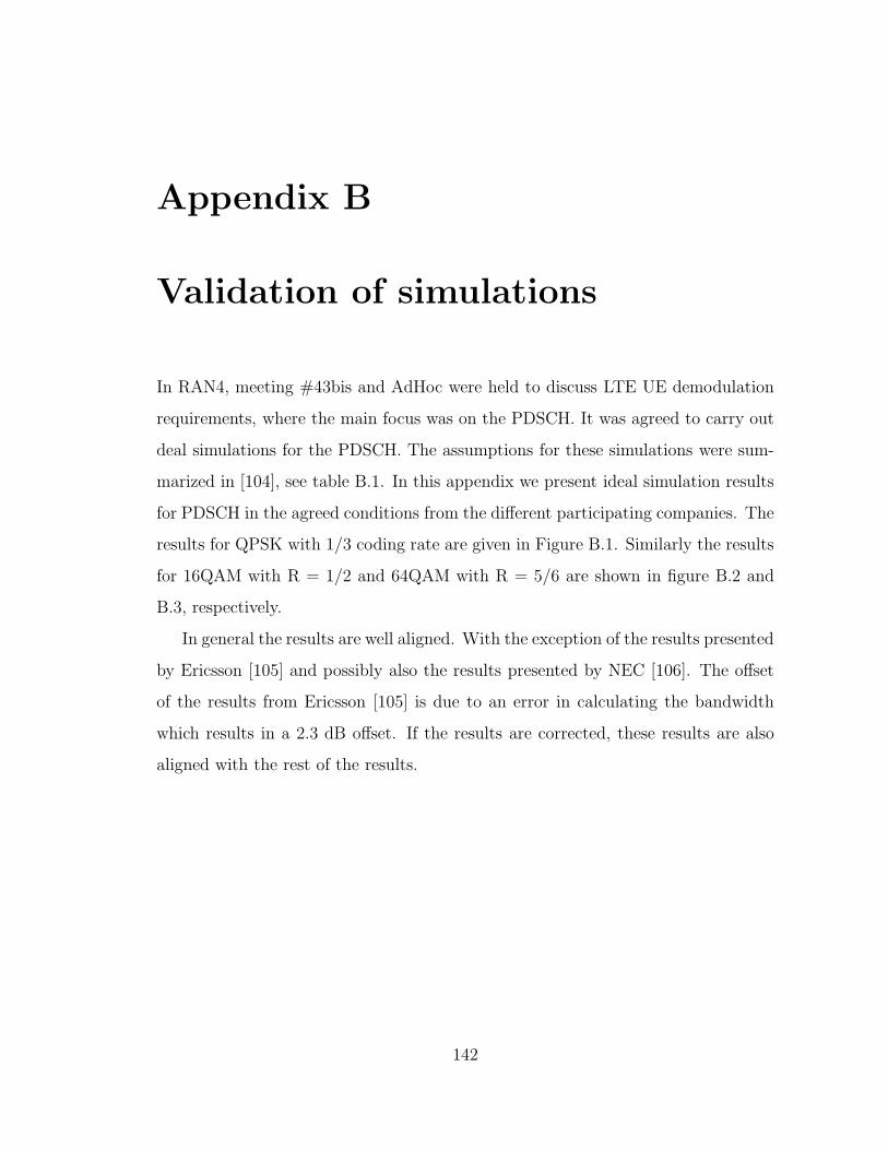
Appendix B
Validation of simulations
In RAN4, meeting #43bis and AdHoc were held to discuss LTE UE demodulation
requirements, where the main focus was on the PDSCH. It was agreed to carry out
deal simulations for the PDSCH. The assumptions for these simulations were sum-
marized in [104], see table B.1. In this appendix we present ideal simulation results
for PDSCH in the agreed conditions from the different participating companies. The
results for QPSK with 1/3 coding rate are given in Figure B.1. Similarly the results
for 16QAM with R = 1/2 and 64QAM with R = 5/6 are shown in figure B.2 and
B.3, respectively.
In general the results are well aligned. With the exception of the results presented
by Ericsson [105] and possibly also the results presented by NEC [106]. The offset
of the results from Ericsson [105] is due to an error in calculating the bandwidth
which results in a 2.3 dB offset. If the results are corrected, these results are also
aligned with the rest of the results.
142
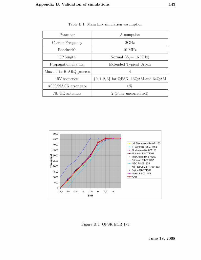
Appendix B. Validation of simulations 143
Table B.1: Main link simulation assumption
Paramter Assumption
Carrier Frequency 2GHz
Bandwidth 10 MHz
CP length Normal (∆f= 15 KHz)
Propagation channel Extended Typical Urban
Max nb tx H-ARQ process 4
RV sequence {0, 1, 2, 3} for QPSK, 16QAM and 64QAM
ACK/NACK error rate 0%
Nb UE antennas 2 (Fully uncorrelated)
0
500
1000
1500
2000
2500
3000
3500
4000
4500
5000
-12,5 -10 -7,5 -5 -2,5 0 2,5 5
SNR
Throughput
LG Electronics R4-071153
IP Wireless R4-071162
Qualcomm R4-071199
Motorola R4-071261
InterDigital R4-071262
Ericsson R4-071297
NEC R4-071325
NTT DoCoMo R4-071363
FujitsuR4-071387
Nokia R4-071405
AAU
Figure B.1: QPSK ECR 1/3
June 18, 2008
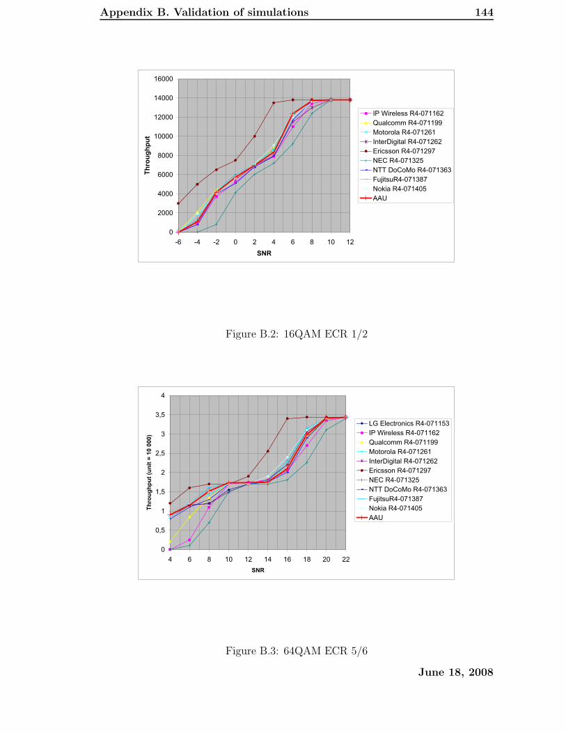
Appendix B. Validation of simulations 144
0
2000
4000
6000
8000
10000
12000
14000
16000
-6 -4 -2 0 2 4 6 8 10 12
SNR
Throughput
IP Wireless R4-071162
Qualcomm R4-071199
Motorola R4-071261
InterDigital R4-071262
Ericsson R4-071297
NEC R4-071325
NTT DoCoMo R4-071363
FujitsuR4-071387
Nokia R4-071405
AAU
Figure B.2: 16QAM ECR 1/2
0
0,5
1
1,5
2
2,5
3
3,5
4
4 6 8 10 12 14 16 18 20 22
SNR
Th
rou
gh
pu
t (u
nit
= 1
0 0
00)
LG Electronics R4-071153
IP Wireless R4-071162
Qualcomm R4-071199
Motorola R4-071261
InterDigital R4-071262
Ericsson R4-071297
NEC R4-071325
NTT DoCoMo R4-071363
FujitsuR4-071387
Nokia R4-071405
AAU
Figure B.3: 64QAM ECR 5/6
June 18, 2008
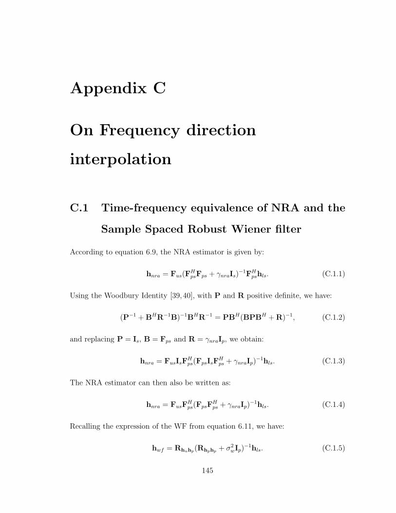
Appendix C
On Frequency direction
interpolation
C.1 Time-frequency equivalence of NRA and the
Sample Spaced Robust Wiener filter
According to equation 6.9, the NRA estimator is given by:
hnra = Fus(FHpsFps + γnraIs)
−1FHpshls. (C.1.1)
Using the Woodbury Identity [39, 40], with P and R positive definite, we have:
(P−1 + BHR−1B)−1BHR−1 = PBH(BPBH + R)−1, (C.1.2)
and replacing P = Is, B = Fps and R = γnraIp, we obtain:
hnra = FusIsFHps(FpsIsF
Hps + γnraIp)
−1hls. (C.1.3)
The NRA estimator can then also be written as:
hnra = FusFHps(FpsF
Hps + γnraIp)
−1hls. (C.1.4)
Recalling the expression of the WF from equation 6.11, we have:
hwf = Rhuhp(Rhphp
+ σ2wIp)
−1hls. (C.1.5)
145
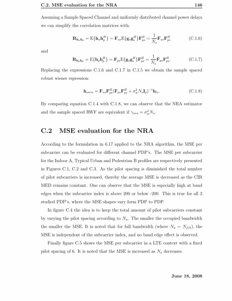
C.2. MSE evaluation for the NRA 146
Assuming a Sample Spaced Channel and uniformly distributed channel power delays
we can simplify the correlation matrices with:
Rhuhp= E{huh
Hp } = FusE{gsg
Hs }FH
ps =1
Ns
FusFHps (C.1.6)
and
Rhphp= E{hph
Hp } = FpsE{gsg
Hs }FH
ps =1
Ns
FpsFHps. (C.1.7)
Replacing the expressions C.1.6 and C.1.7 in C.1.5 we obtain the sample spaced
robust wiener espression:
hssrw = FusFHps(FpsF
Hps + σ2
wNsIp)−1hls. (C.1.8)
By comparing equation C.1.4 with C.1.8, we can observe that the NRA estimator
and the sample spaced RWF are equivalent if γnra = σ2wNs.
C.2 MSE evaluation for the NRA
According to the formulation in 6.17 applied to the NRA algorithm, the MSE per
subcarrier can be evaluated for different channel PDP’s. The MSE per subcarrier
for the Indoor A, Typical Urban and Pedestrian B profiles are respectively presented
in Figures C.1, C.2 and C.3. As the pilot spacing is diminished the total number
of pilot subcarriers is increased, thereby the average MSE is decreased as the CIR
MED remains constant. One can observe that the MSE is especially high at band
edges when the subcarrier index is above 200 or below -200. This is true for all 3
studied PDP’s, where the MSE shapes vary form PDP to PDP.
In figure C.4 the idea is to keep the total amount of pilot subcarriers constant
by varying the pilot spacing according to Nu. The smaller the occupied bandwidth
the smaller the MSE. It is noted that for full bandwidth (where Nu = Nfft), the
MSE is independent of the subcarrier index, and no band edge effect is observed.
Finally figure C.5 shows the MSE per subcarrier in a LTE context with a fixed
pilot spacing of 6. It is noted that the MSE is increased as Nu decreases.
June 18, 2008
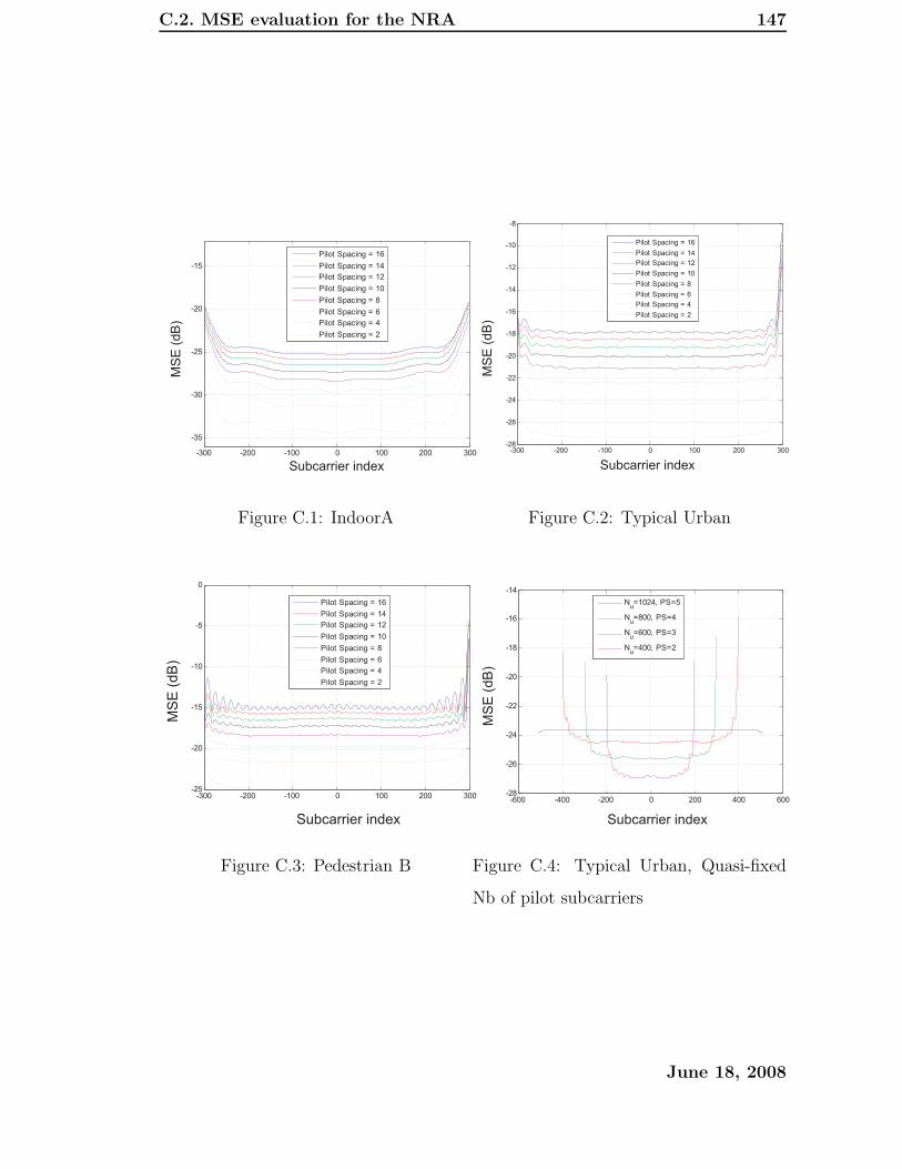
C.2. MSE evaluation for the NRA 147
-300 -200 -100 0 100 200 300
-35
-30
-25
-20
-15
MML 16QAM Nfft=1024 Nu=600 PPat=1
POff=2 SNR=10 dB gamma=wiener Chan=5 Ng=opt
Subcarrier Index
MS
E(d
B)
Pilot Spacing = 16
Pilot Spacing = 14
Pilot Spacing = 12
Pilot Spacing = 10
Pilot Spacing = 8
Pilot Spacing = 6
Pilot Spacing = 4
Pilot Spacing = 2
Subcarrier index
MS
E(d
B)
Figure C.1: IndoorA
Subcarrier index
MS
E(d
B)
-300 -200 -100 0 100 200 300-28
-26
-24
-22
-20
-18
-16
-14
-12
-10
-8
Subcarrier Index
MS
E(d
B)
MML 16QAM Nfft=1024 Nu=600 PPat=1
POff=0 SNR=10 dB gamma=wiener Chan=8 Ng=opt
Pilot Spacing = 16
Pilot Spacing = 14
Pilot Spacing = 12
Pilot Spacing = 10
Pilot Spacing = 8
Pilot Spacing = 6
Pilot Spacing = 4
Pilot Spacing = 2
Figure C.2: Typical Urban
Subcarrier index
MS
E(d
B)
-300 -200 -100 0 100 200 300-25
-20
-15
-10
-5
0
Subcarrier Index
MS
E(d
B)
MML 16QAM Nfft=1024 Nu=600 PPat=1
POff=0 SNR=10 dB gamma=wiener Chan=2 Ng=opt
Pilot Spacing = 16
Pilot Spacing = 14
Pilot Spacing = 12
Pilot Spacing = 10
Pilot Spacing = 8
Pilot Spacing = 6
Pilot Spacing = 4
Pilot Spacing = 2
Figure C.3: Pedestrian B
Subcarrier index
MS
E(d
B)
-600 -400 -200 0 200 400 600-28
-26
-24
-22
-20
-18
-16
-14
Subcarrier Index
MS
E(d
B)
MML 16QAM Nfft=1024 Nu=400 PPat=1 PSpac=2
POff=0 SNR=10 dB gamma=wiener Chan=8 Ng=opt
Nu=1024, PS=5
Nu=800, PS=4
Nu=600, PS=3
Nu=400, PS=2
Figure C.4: Typical Urban, Quasi-fixed
Nb of pilot subcarriers
June 18, 2008
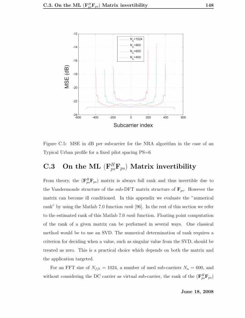
C.3. On the ML (FHpsFps) Matrix invertibility 148
Subcarrier index
MS
E(d
B)
-600 -400 -200 0 200 400 600-24
-22
-20
-18
-16
-14
-12
Subcarrier Index
MS
E(d
B)
MML 16QAM Nfft=1024 PPat=1 PSpac=6
POff=0 SNR=10 dB gamma=wiener Chan=8 Ng=opt
Nu=1024
Nu=800
Nu=600
Nu=400
Figure C.5: MSE in dB per subcarrier for the NRA algorithm in the case of an
Typical Urban profile for a fixed pilot spacing PS=6
C.3 On the ML (FHpsFps) Matrix invertibility
From theory, the (FHpsFps) matrix is always full rank and thus invertible due to
the Vandermonde structure of the sub-DFT matrix structure of Fps. However the
matrix can become ill conditioned. In this appendix we evaluate the ”numerical
rank” by using the Matlab 7.0 function rank [96]. In the rest of this section we refer
to the estimated rank of this Matlab 7.0 rank function. Floating point computation
of the rank of a given matrix can be performed in several ways. One classical
method would be to use an SVD. The numerical determination of rank requires a
criterion for deciding when a value, such as singular value from the SVD, should be
treated as zero. This is a practical choice which depends on both the matrix and
the application targeted.
For an FFT size of Nfft = 1024, a number of used sub-carriers Nu = 600, and
without considering the DC carrier as virtual sub-carrier, the rank of the (FHpsFps)
June 18, 2008
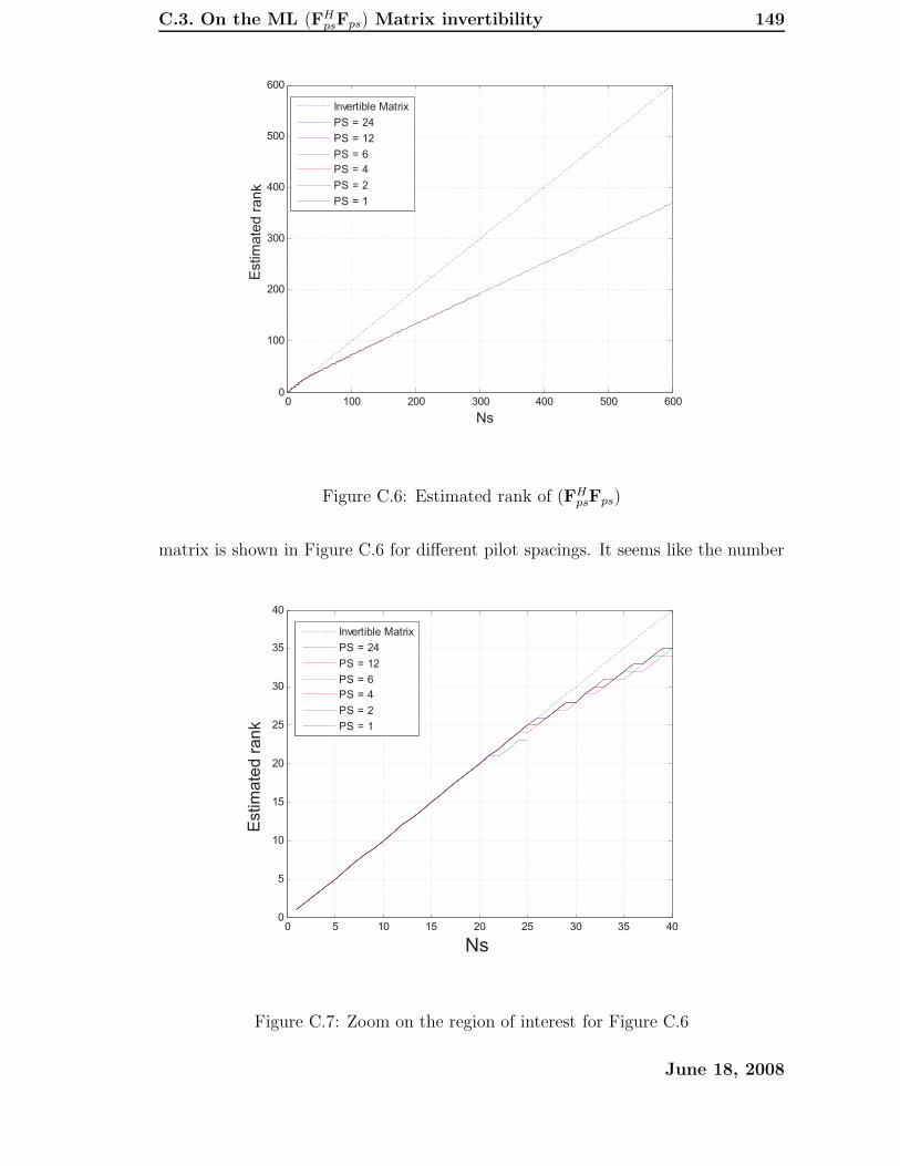
C.3. On the ML (FHpsFps) Matrix invertibility 149
0 100 200 300 400 500 6000
100
200
300
400
500
600
CIR length (samples)
Rank
Rank of FpgH
? Fpg. Nf f t
= 1024, Nu
= 600, DC carrier Used
Invertible Matrix
PS = 24
PS = 12
PS = 6
PS = 4
PS = 2
PS = 1
Ns
Estim
ate
dra
nk
Figure C.6: Estimated rank of (FHpsFps)
matrix is shown in Figure C.6 for different pilot spacings. It seems like the number
0 5 10 15 20 25 30 35 400
5
10
15
20
25
30
35
40
CIR length (samples)
Rank
Rank of FpgH
? Fpg. Nff t
= 1024, Nu
= 600, DC carrier Used
Invertible Matrix
PS = 24
PS = 12
PS = 6
PS = 4
PS = 2
PS = 1
Estim
ate
d r
ank
Ns
Figure C.7: Zoom on the region of interest for Figure C.6
June 18, 2008
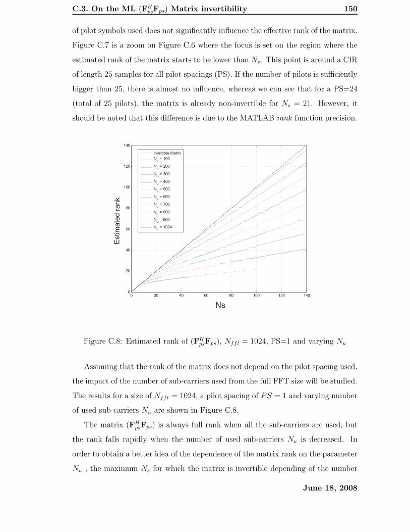
C.3. On the ML (FHpsFps) Matrix invertibility 150
of pilot symbols used does not significantly influence the effective rank of the matrix.
Figure C.7 is a zoom on Figure C.6 where the focus is set on the region where the
estimated rank of the matrix starts to be lower than Ns. This point is around a CIR
of length 25 samples for all pilot spacings (PS). If the number of pilots is sufficiently
bigger than 25, there is almost no influence, whereas we can see that for a PS=24
(total of 25 pilots), the matrix is already non-invertible for Ns = 21. However, it
should be noted that this difference is due to the MATLAB rank function precision.
0 20 40 60 80 100 120 1400
20
40
60
80
100
120
140
CIR Length (samples)
Rank
Rank of FpgH
?Fpg
. Nf f t
= 1024, Pilot Spacing = 1, DC carrier used
Invertible Matrix
Nu
= 100
Nu
= 200
Nu
= 300
Nu
= 400
Nu
= 500
Nu
= 600
Nu
= 700
Nu
= 800
Nu
= 900
Nu
= 1024
Estim
ate
d r
an
k
Ns
Figure C.8: Estimated rank of (FHpsFps), Nfft = 1024, PS=1 and varying Nu
Assuming that the rank of the matrix does not depend on the pilot spacing used,
the impact of the number of sub-carriers used from the full FFT size will be studied.
The results for a size of Nfft = 1024, a pilot spacing of PS = 1 and varying number
of used sub-carriers Nu are shown in Figure C.8.
The matrix (FHpsFps) is always full rank when all the sub-carriers are used, but
the rank falls rapidly when the number of used sub-carriers Nu is decreased. In
order to obtain a better idea of the dependence of the matrix rank on the parameter
Nu , the maximum Ns for which the matrix is invertible depending of the number
June 18, 2008
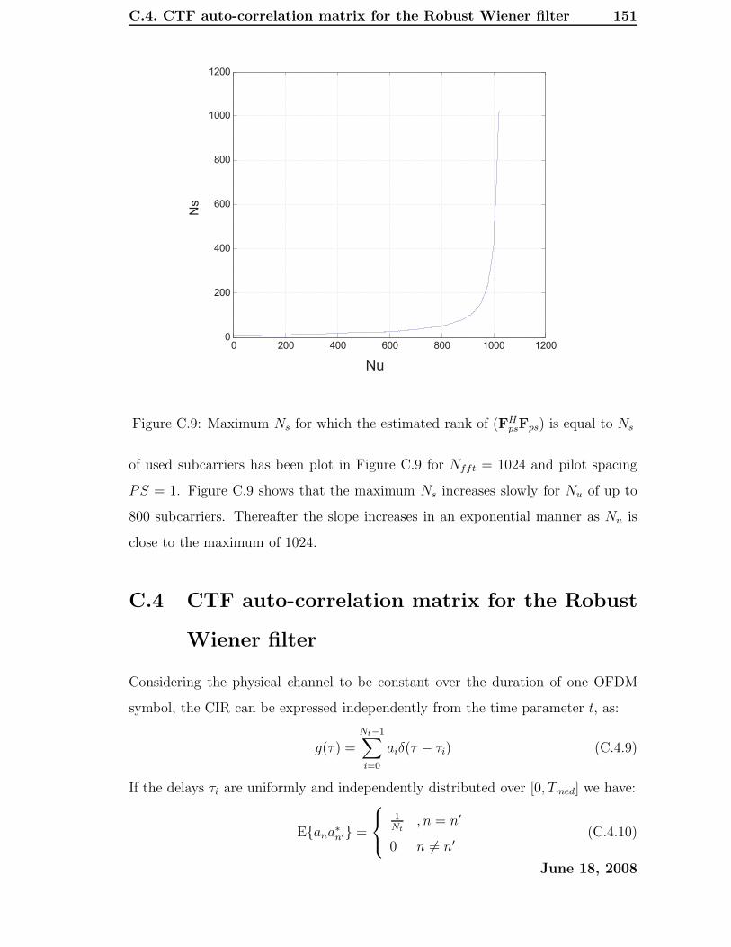
C.4. CTF auto-correlation matrix for the Robust Wiener filter 151
0 200 400 600 800 1000 12000
200
400
600
800
1000
1200
Nu
Ng
Maximum Ng
for invertible FpgH
?Fpg
Ns
Nu
Figure C.9: Maximum Ns for which the estimated rank of (FHpsFps) is equal to Ns
of used subcarriers has been plot in Figure C.9 for Nfft = 1024 and pilot spacing
PS = 1. Figure C.9 shows that the maximum Ns increases slowly for Nu of up to
800 subcarriers. Thereafter the slope increases in an exponential manner as Nu is
close to the maximum of 1024.
C.4 CTF auto-correlation matrix for the Robust
Wiener filter
Considering the physical channel to be constant over the duration of one OFDM
symbol, the CIR can be expressed independently from the time parameter t, as:
g(τ) =Nt−1∑
i=0
aiδ(τ − τi) (C.4.9)
If the delays τi are uniformly and independently distributed over [0, Tmed] we have:
E{ana∗n′} =
1Nt
, n = n′
0 n 6= n′(C.4.10)
June 18, 2008

C.5. On the optimal choice of γ for the NRA 152
The CTF is defined as:
h[k] =
Nt−1∑
i=0
aie−j2π k
Nfftτi
(C.4.11)
The CTF auto-correlation matrix is expressed as:
Rhh[k, k′] = E{h[k]h∗[k′]} (C.4.12)
= E{
Nt−1∑
i1=0
ai1e−j2π k
Nfftτi1
Nt−1∑
i2=0
a∗i2ej2π k′
Nfftτi2} (C.4.13)
=1
Nt
Nt−1∑
i=0
E{e−j2π
(k−k′)Nfft
τi} (C.4.14)
We observe that the probability density function of τi is:
f(τi) =
1Tmed
, τi ∈ [0, Tmed]
0 , else.(C.4.15)
It follows,
Rhh[k, k′] =1
Nt
Nt−1∑
i=0
∫ Tmed
0
e−j2π k−k′
Nfftτi
Tmed
dτi (C.4.16)
=1
Nt
Nt−1∑
i=0
[
−Nffte−j2π k−k′
Nfftτi
j2π(k − k′)Tmed
]Tmed
0
(C.4.17)
=1
Nt
Nt−1∑
i=0
[
−Nffte−j2π k−k′
NfftTmed
j2π(k − k′)Tmed
+Nfft
j2π(k − k′)Tmed
]
(C.4.18)
=Nfft
j2π(k − k′)Tmed
(1 − e−j2π k−k′
NfftTmed
) (C.4.19)
(C.4.20)
Finally we have:
Rhh[k, k′] =1 − e
−j2π(k−k′)Nfft
Tmed
j2π (k−k′)Nfft
Tmed
. (C.4.21)
C.5 On the optimal choice of γ for the NRA
According to the formulation of equation 6.9 we have:
hnra = Fus(FHpsFps + γIs)
−1FHpshls. (C.5.22)
June 18, 2008
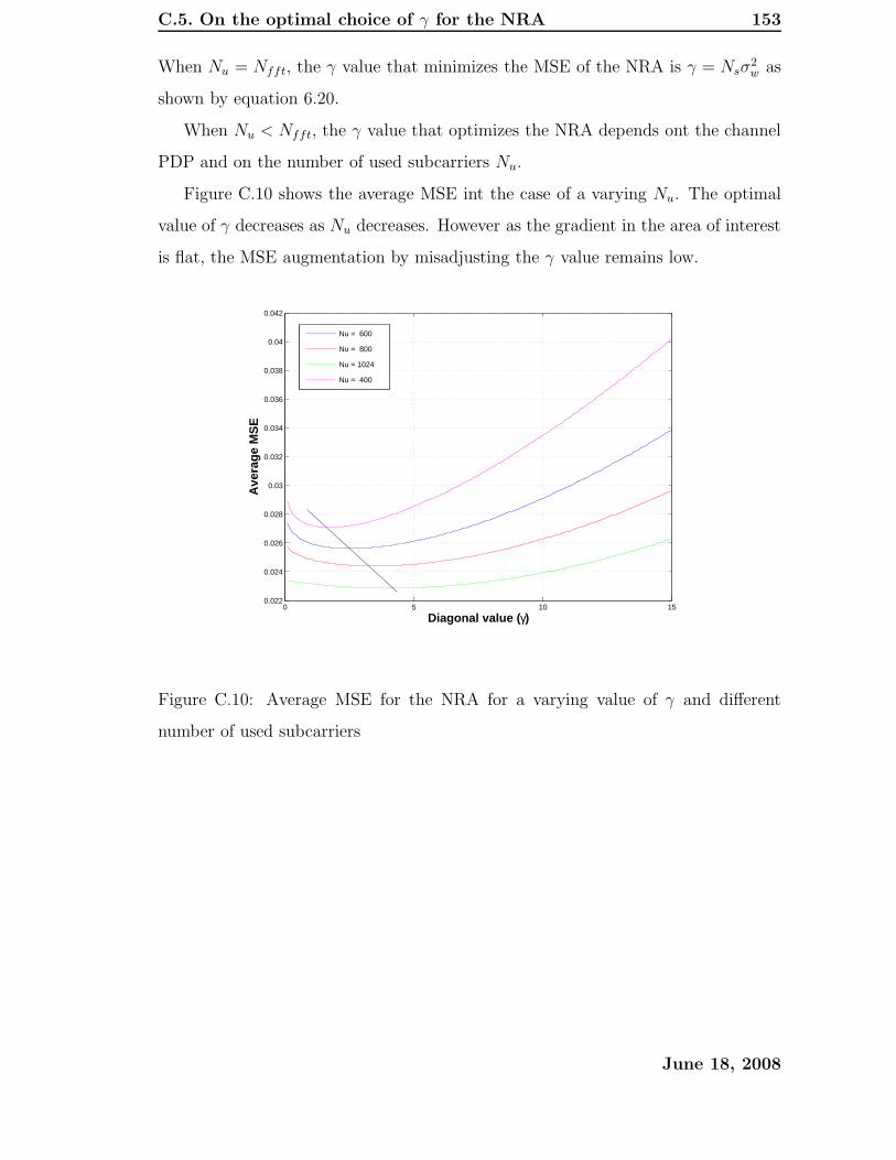
C.5. On the optimal choice of γ for the NRA 153
When Nu = Nfft, the γ value that minimizes the MSE of the NRA is γ = Nsσ2w as
shown by equation 6.20.
When Nu < Nfft, the γ value that optimizes the NRA depends ont the channel
PDP and on the number of used subcarriers Nu.
Figure C.10 shows the average MSE int the case of a varying Nu. The optimal
value of γ decreases as Nu decreases. However as the gradient in the area of interest
is flat, the MSE augmentation by misadjusting the γ value remains low.
0 5 10 150.022
0.024
0.026
0.028
0.03
0.032
0.034
0.036
0.038
0.04
0.042
Diagonal value ( γ)
Ave
rage
MS
E
Nu = 600
Nu = 800
Nu = 1024
Nu = 400
Figure C.10: Average MSE for the NRA for a varying value of γ and different
number of used subcarriers
June 18, 2008

C.6. Evaluation of the Low-Rank approximation of the Robust Wienerfilter for different PDPs 154
C.6 Evaluation of the Low-Rank approximation
of the Robust Wiener filter for different PDPs
The Singular Value Decomposition of the channel auto-covariance matrix Rhh of
the RWF from equation 6.30 is given by:
Rhh = UΛUH , (C.6.23)
with U being an (Nfft · Nfft) unitary matrix containing the singular vectors. The
Λ diagonal matrix of dimension (Nfft ·Nfft) contains the singular values λ1 ≥ λ2 ≥
λ3... ≥ λNfftof Rhh.
The rank-e estimator from [68] is given by:
h(e)svd = U∆eU
Hhls. (C.6.24)
∆e is a diagonal matrix with entries given by:
∆e[n, n′] =
λn
λn+βσ2w
{n = n′} ∧ {n = 1, 2, ..., Ne}
0 {n = n′} ∧ {n ≥ Ne + 1}
0 n 6= n′,
(C.6.25)
where β is modulation dependent (i.e. for 16QAM β = 179), and λn is the nth singular
value.
The complexity of this rank-e estimator is of the order O(Ne · (2Nfft + Ne))
however in a system with Nu used subcarriers and Np pilot subcarriers this becomes
O(Ne · (Nu +Ne +Np)). This shows a strong dependency on the rank Ne chosen for
the estimator.
In order to quantify the rank order to be chosen, different CIR MED length
are chosen for the RWF. The magnitude of the ordered singular values of Rhh are
depicted in Figures C.11 and C.12.
The blue circles represent the CIR MED length in samples. It is clear to see a
strong drop of the singular values as soon as the index n is slightly larger than the
CIR MED.
June 18, 2008
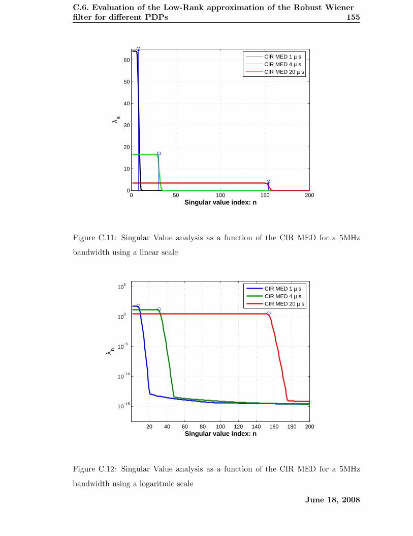
C.6. Evaluation of the Low-Rank approximation of the Robust Wienerfilter for different PDPs 155
0 50 100 150 2000
10
20
30
40
50
60
Singular value index: n
λ n
CIR MED 1 µ sCIR MED 4 µ sCIR MED 20 µ s
Figure C.11: Singular Value analysis as a function of the CIR MED for a 5MHz
bandwidth using a linear scale
20 40 60 80 100 120 140 160 180 200
10−15
10−10
10−5
100
105
Singular value index: n
λ n
CIR MED 1 µ sCIR MED 4 µ sCIR MED 20 µ s
Figure C.12: Singular Value analysis as a function of the CIR MED for a 5MHz
bandwidth using a logaritmic scale
June 18, 2008
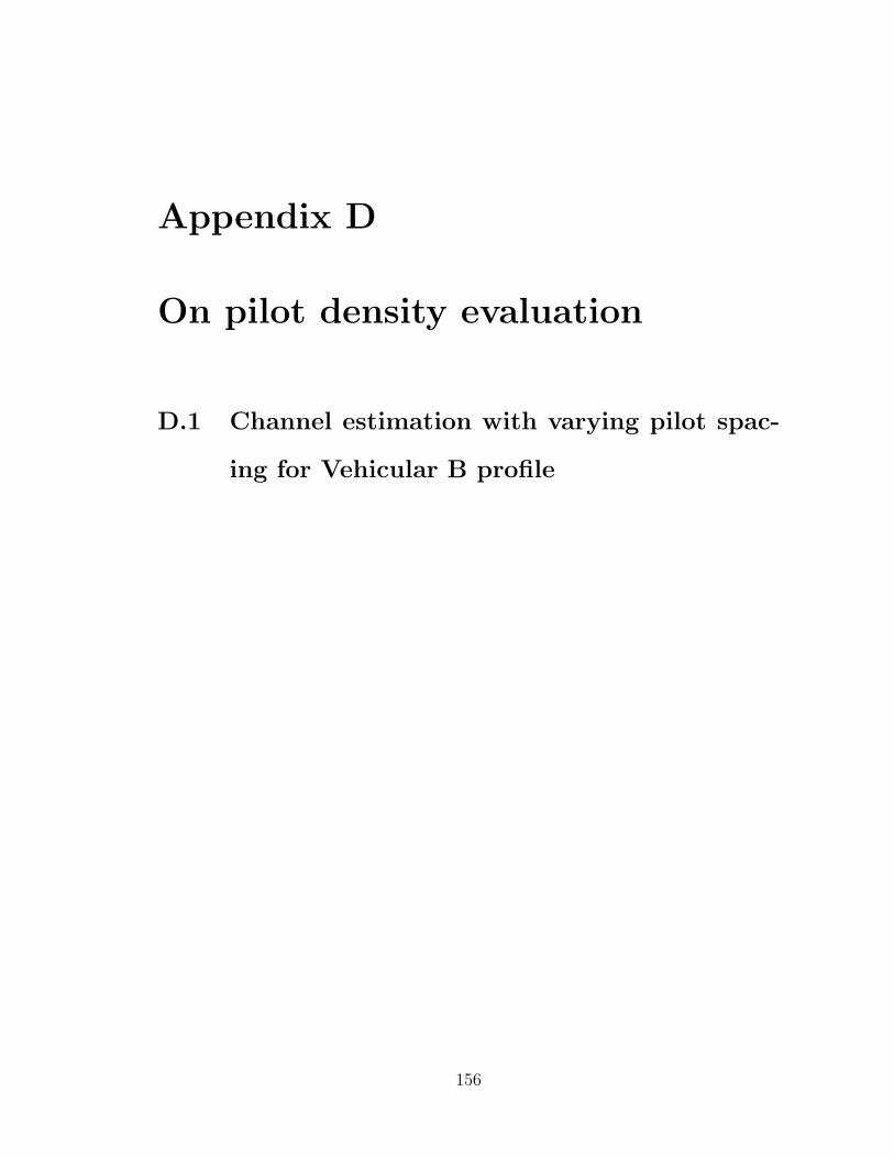
Appendix D
On pilot density evaluation
D.1 Channel estimation with varying pilot spac-
ing for Vehicular B profile
156
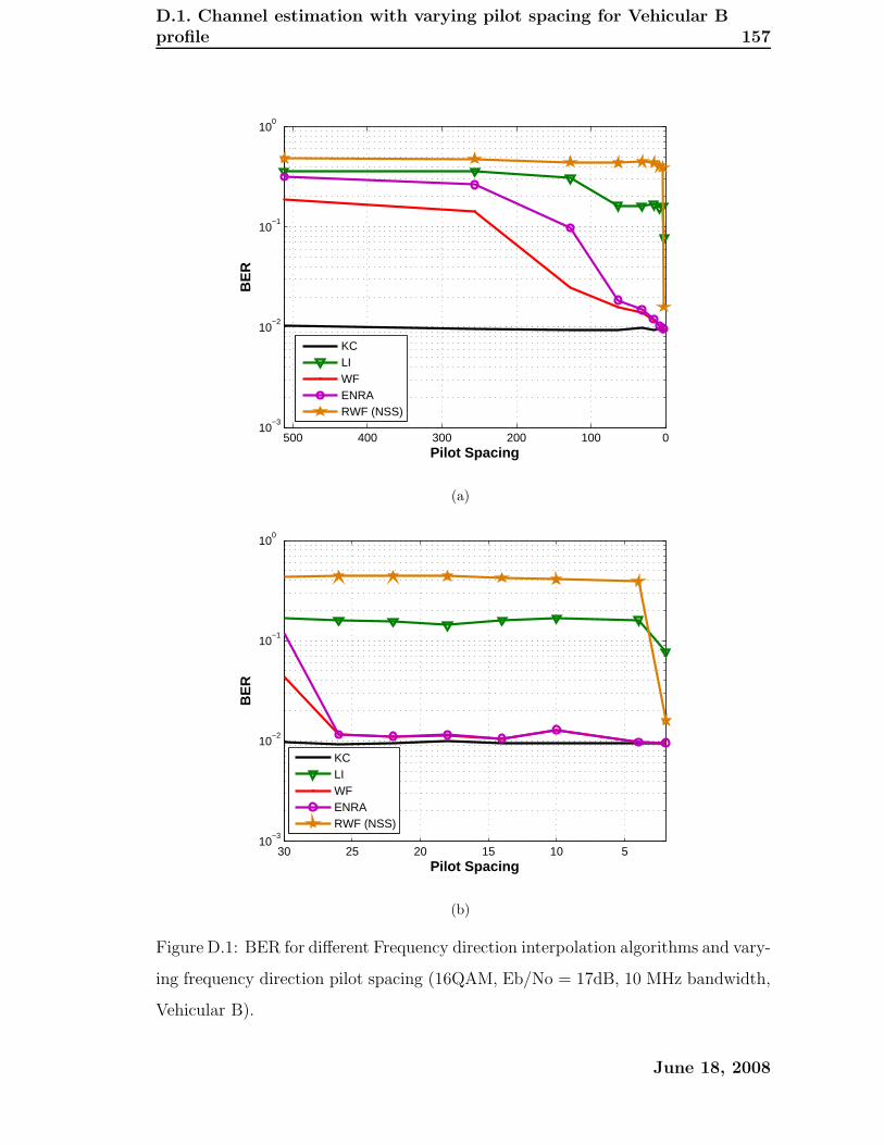
D.1. Channel estimation with varying pilot spacing for Vehicular Bprofile 157
010020030040050010
−3
10−2
10−1
100
Pilot Spacing
BE
R
KCLIWFENRARWF (NSS)
(a)
5101520253010
−3
10−2
10−1
100
Pilot Spacing
BE
R
KCLIWFENRARWF (NSS)
(b)
Figure D.1: BER for different Frequency direction interpolation algorithms and vary-
ing frequency direction pilot spacing (16QAM, Eb/No = 17dB, 10 MHz bandwidth,
Vehicular B).
June 18, 2008

D.2. Spectral Efficiency evaluation for different pilot schemes 158
D.2 Spectral Efficiency evaluation for different pi-
lot schemes
−10 −5 0 5 10 15 20 25 300
0.5
1
1.5
2
2.5
3
3.5
4
SNR (dB)
Spe
ctra
l Effi
cien
cy (
bits
/s/H
z)
QPSK 0.17QPSK 0.33QPSK 0.50QPSK 0.6716QAM 0.5016QAM 0.6716QAM 0.7564QAM 0.5064QAM 0.6764QAM 0.7564QAM 0.80
Figure D.2: Spectral efficiency for a 10 MHz bandwidth, Typical Urban PDP, dif-
ferent ECR, Pilot scheme P1 at 3kmph, WF in frequency direction and LI in time
direction interpolation
−10 −5 0 5 10 15 20 25 30 350
0.1
0.2
0.3
0.4
0.5
0.6
0.7
0.8
SNR (dB)
Spe
ctra
l Effi
cien
cy (
bits
/s/H
z)
QPSK 0.17QPSK 0.33QPSK 0.50QPSK 0.6716QAM 0.5016QAM 0.6716QAM 0.7564QAM 0.5064QAM 0.6764QAM 0.7564QAM 0.80
Figure D.3: Spectral efficiency for a 10 MHz bandwidth, Typical Urban PDP, dif-
ferent ECR, Pilot scheme P1 at 300kmph, WF in frequency direction and LI in time
direction interpolation
June 18, 2008
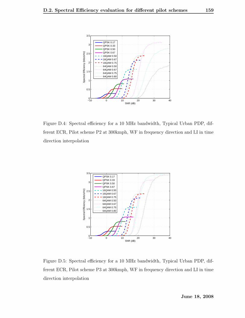
D.2. Spectral Efficiency evaluation for different pilot schemes 159
−10 0 10 20 30 400
0.5
1
1.5
2
2.5
3
3.5
SNR (dB)
Spe
ctra
l Effi
cien
cy (
bits
/s/H
z)
QPSK 0.17QPSK 0.33QPSK 0.50QPSK 0.6716QAM 0.5016QAM 0.6716QAM 0.7564QAM 0.5064QAM 0.6764QAM 0.7564QAM 0.80
Figure D.4: Spectral efficiency for a 10 MHz bandwidth, Typical Urban PDP, dif-
ferent ECR, Pilot scheme P2 at 300kmph, WF in frequency direction and LI in time
direction interpolation
−10 0 10 20 30 400
0.5
1
1.5
2
2.5
3
3.5
SNR (dB)
Spe
ctra
l Effi
cien
cy (
bits
/s/H
z)
QPSK 0.17QPSK 0.33QPSK 0.50QPSK 0.6716QAM 0.5016QAM 0.6716QAM 0.7564QAM 0.5064QAM 0.6764QAM 0.7564QAM 0.80
Figure D.5: Spectral efficiency for a 10 MHz bandwidth, Typical Urban PDP, dif-
ferent ECR, Pilot scheme P3 at 300kmph, WF in frequency direction and LI in time
direction interpolation
June 18, 2008
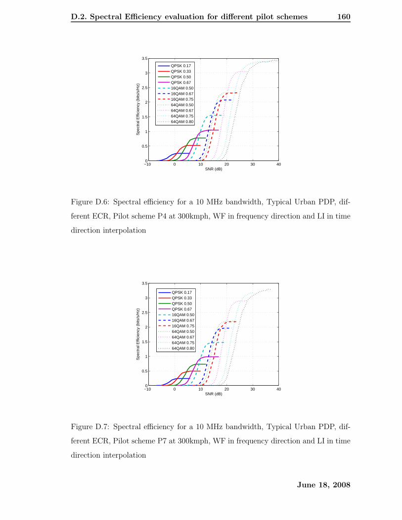
D.2. Spectral Efficiency evaluation for different pilot schemes 160
−10 0 10 20 30 400
0.5
1
1.5
2
2.5
3
3.5
SNR (dB)
Spe
ctra
l Effi
cien
cy (
bits
/s/H
z)
QPSK 0.17QPSK 0.33QPSK 0.50QPSK 0.6716QAM 0.5016QAM 0.6716QAM 0.7564QAM 0.5064QAM 0.6764QAM 0.7564QAM 0.80
Figure D.6: Spectral efficiency for a 10 MHz bandwidth, Typical Urban PDP, dif-
ferent ECR, Pilot scheme P4 at 300kmph, WF in frequency direction and LI in time
direction interpolation
−10 0 10 20 30 400
0.5
1
1.5
2
2.5
3
3.5
SNR (dB)
Spe
ctra
l Effi
cien
cy (
bits
/s/H
z)
QPSK 0.17QPSK 0.33QPSK 0.50QPSK 0.6716QAM 0.5016QAM 0.6716QAM 0.7564QAM 0.5064QAM 0.6764QAM 0.7564QAM 0.80
Figure D.7: Spectral efficiency for a 10 MHz bandwidth, Typical Urban PDP, dif-
ferent ECR, Pilot scheme P7 at 300kmph, WF in frequency direction and LI in time
direction interpolation
June 18, 2008