GEOPHYSICAL RESEARCH LETTERS, VOL. 35, L09301, DOI:10.1029/2008GL033256, 2008

An improved neighborhood algorithm: parameter conditions

and dynamic scaling

M. WatheletLGIT, IRD, CNRS, Universite Joseph Fourier, BP 53, 38041 Grenoble Cedex 9, France.

The Neighborhood Algorithm (NA) is a popular di-rect search inversion technique. For dispersion curve in-version, physical conditions between parameters Vs andVp (linked by Poisson’s ratio) may limit the parameterspace with complex boundaries. Other conditions maycome from prior information about the geological struc-ture. Irregular limits are not natively handled by classi-cal search algorithms. In this paper, we extend the NAformulation to such parameter spaces. For problems af-fected by non-uniqueness, the ideal solution is made ofthe ensemble of all models that equally fits the data andprior information. Hence, a powerful exploration tool isrequired. Exploiting the properties of the Voronoi cells,we show that a dynamic scaling of the parameters duringthe convergence to the solutions drastically improves theexploration.

1. Introduction

Inversion techniques are widespread in geophysics asattested by the number of scientific activities dealing withtheir development and their application, mostly sincethe beginning of the computer era. Inversion tools in-clude linearized methods (Nolet [1981]; Tarantola [1987])and direct search techniques (Sen and Stoffa [1991]; Lo-max and Snieder [1994]) that gained success during thenineties parallel to the development of the power of deskcomputers. For inversion problems with a reduced num-ber of unknowns, direct search methods are probably bestsuited because of their ability to correctly map the un-certainties of the problem in the case of non-uniqueness(distinct equivalent solutions).

The Neighborhood Algorithm (NA, Sambridge [1999])is a stochastic direct search method that belongs to thesame familly as Genetic Algorithms (GA, Lomax andSnieder [1994]) or Simulated Annealing (SA, Sen andStoffa [1991]). Compared to a basic Monte Carlo sam-pling, these approaches try to guide the random genera-tion of samples by the results obtained so far on previ-ous samples. The areas of the parameter space whereno interesting solution can be found are less sampledthan promising areas. All methods require several tuningparameters to control the balance between exploitationand exploration, i.e. between a quick convergence to aminimum of the misfit function and slow investigation ofnearly all local minima to find the global one or identifyequivalent minima.

NA makes use of Voronoi cells to model the misfitfunction across the parameter space. The misfit func-tion is supposed to be known for ns0 samples randomlydistributed or not over the parameter space. A Voronoi

Copyright 2008 by the American Geophysical Union.0094-8276/08/2008GL033256$5.00

cell centered around one of these samples is the nearestneighbor region defined under a suitable distance norm(usually Euclidean). The union of all cells with a low mis-fit is the area of interest where new samples with smallmisfits are expected. The size of this ensemble is de-fined by the tuning parameter nr (number of best cellsto consider). Sambridge [1999] proposed a simple butvery efficient way to generate new random samples in-side a Voronoi cell based on a Gibbs sampler. ns (secondtuning parameter) new samples are generated and addedto the original population (ns/nr samples per cell areadded). The geometry of the initial Voronoi cells aremodified to include these new ns samples. The processis repeated itmax (last tuning parameter) times until anacceptable sampling of the solution is obtained.

We take the classical inversion of shear wave velocityprofiles from surface wave dipersion curves as an exam-ple. We first show that a good parameterization requiresa parameter space with irregular conditions whereas theoriginal NA is limited to an hyper-box. A suitable mod-ification of the NA kernel is proposed. Secondly, we im-prove the exploration capabilities of NA by playing onparameter scales. It is particulary usefull for inversionproblems affected by non-uniqueness.

2. Searching inside irregular boundaries

In tabular ground structures (made of homogeneousand horizontal layers), typically used for the computationof dispersion curves, four parameters can fully describe anelastic layer: Vs, H (thickness), Vp, and ρ (density). Theyare given by decreasing influence, especially the densitycan be considered as constant. Vs and Vp are directlyrelated through the Poisson’s Ratio(ν) which generallyranges from 0.2 to 0.5 in the nature. Historically, theeffect of Vp over the dispersion curve has been consideredas negligible. Nevertheless, Wathelet [2005] showed thatthis is not true for all Poisson’s ratio values, particularlyfor those encountered for hard rocks (below 0.3).

2.1. Parameters of a layer: Vp, Vs, or ν?

The usual approach, designed for linearized methods,divides the tabular structure into homogeneous layerswith fixed thicknesses. Inside each layer, two options aregenerally available (Herrmann [1994]): fixing Vp or ν. Vs

is left as the unique free parameter in all cases. Vp pro-files measured by refraction experiments have their ownuncertainties as recently recalled by Ivanov et al. [2006],and fixing definitively Vp to some arbitrary value mayartificially reduce the range of possible solutions. ThusWathelet et al. [2004] introduced another parameteriza-tion with two free parameters per layer: Vp and the ratioVs/Vp, that has the advantage to keep all parameters tophysically acceptable ranges. However, Vs is the most im-portant parameter for surface wave problems. Not havinga direct control over this parameter during the inversionis penalizing in most situations. Furthermore, in the con-text of stochastic inversion schemes, Vs is obtained bya non-linear combination of two random variables withuniform distributions (Vp and Vs/Vp). Hence, the prior

1

X - 2 WATHELET: PARAMETER CONDITIONS AND DYNAMIC SCALING

distribution of Vs is not uniform. Though uniform distri-butions cannot be considered as the total absence of priorinformation about a parameter value (Edwards [1992]), itis certainly closer to our prior knowledge than any uncon-trolled and non uniform distribution (i.e. that supportssome particular values rather than others) introduced bythis non-linear combination used for computing Vs. Theoptimum parameterization would be Vs and Vp as freeparameters compatible with Poisson’s ratio conditions.

2.2. Freeing thicknesses

With the increasing success of stochastic inversionmethods, velocities and thicknesses are both set as freeparameters (e.g. Wathelet et al. [2004], Picozzi et al.[2005]), which greatly helps reducing the number of de-grees of freedom (Scherbaum et al. [2003]). Nevertheless,in a stack of N layers, the depth of the half-space top isthus the sum of N random variables with a uniform dis-tribution and a finite variance. Using the Central LimitTheorem, the prior distribution of the bottom of the N th

layer tends towards a Gaussian. Hence, considering alarge number of layers leads to generate models stick-ing around a median depth and not exploring any otherdepths for the deeper layers. For instance, with four lay-ers above a half-space, the top of the half-space has only5% chance to lie out of 4 standard deviations (from 85to 315 m if the total possible range is from 0 to 400 m, areduction of 42.5%). A possible solution would be to setup depth rather than thickness parameters. To generatevalid ground models, the depth parameters must havegreater values for deeper layers than for shallow ones,requiring some additional conditions.

2.3. Low velocity zones (LVZ)

Surface wave methods, especially for active source ex-periments, are usually appreciated because they can in-vestigate soft layers covered by stiffer ones (e.g. Rydenand Park [2004]). LVZs may induce problems in the for-ward computation of the dispersion curve at high fre-quency (relative to the model structure): crossing modescan be encountered. Quick and straightforward algo-rithms are usually not suitable. Hence, during the ran-dom generation of models, the dispersion curve may beimpossible to compute for some particular Vs profileswith LVZs. It defines an irregular limit to the param-eter space that we can only estimate by trial and error.Lack of precision defining this complex boundary mayeventually shadow parts of the parameter space contain-ing low misfit solutions. Another aspect of LVZs is thatthey can potentially increase the number of possible so-lutions and the non-uniqueness of the problem. If ourprior knowledge about the geological structure does notjustify the presence of any LVZ, it would be interestingto generate random Vs profiles without LVZ, requiring asimple condition at each interface.

2.4. Implementation

In the above discussion, reviewing three aspects ofthe parameterization of tabular ground structures clearlyshows the need for an inversion algorithm confined in aparameter space with complex boundaries. We assumethe parameter space bounded by an hyper-box (classicallimits) and by irregular limits, due to physical conditions,numerical limitations or prior information (Fig. 1). Themisfit computation is possible only inside the intersec-tion of these two ensembles. By contrast with the hyper-

box, the irregular limits may have no explicit definition(e.g. failure of the dispersion curve computation in caseof strong LVZs).

At the beginning of each iteration, the original NAgenerates ns new models inside nr cells. The corre-sponding misfits are computed in a second step by auser-provided function returning a floating-point value(implementation of the forward problem). To correctlyhandle failures of the misfit computation, we propose afunction which returns an additional boolean value (trueif it is a valid model). The generation of models by theGibbs sampler must be integrated with the computationof misfits. nc = ns/nr new samples are produced for eachcell of the active region (union of all best nr cells). If nc

is not an integer, it is rounded down and the remainingmodels are randomly distributed on the active cells. Foreach cell (repeated nc times), the Gibbs sampler is usedto generate a model and its misfit is directly computed.In case of success, the model is accepted the same wayas in the original algorithm. If not, the returned misfitis ignored (it can be 0) and another model is randomlygenerated inside the cell until success. The original rigidconcept of iterations has also been modified in a recentparallelization of the NA core (Rickwood and Sambridge[2006]). Our conditional solution could be also developedfor the parallel algorithm.

When the active region is close to one of the complexboundaries, Voronoi cells where new samples are gener-ated can be cut by one of them and only a small percent-age of their multi-dimensional volume may be includedinside the valid region (e.g. cell l in Fig. 1). Thus,there might be only very little chance to generate onegood sample even after a lot of trials. A way of solvingthis problem is to count all accepted and rejected modelsper cell. If the proportion of rejected models exceed athreshold (e.g. 90%), the cell is thrown away from theactive region and replaced by the cell with the best misfitcurrently outside the active region.

When there are a lot of conditions to satisfy, this ran-dom generator is not very efficient. A lot of invalid mod-els must be rejected before accepting just one. If an ex-plicit definition of the conditions is available, the Gibbssampler can be modified to always return a valid model.For each parameter we define a list of conditions. A con-dition is a C++ object (a data structure with dedicatedfunctions) that links several parameters together (it canbe as simple as p1 < p2). It has a mandatory functionthat returns the admissible range for each of its parame-ters, keeping all others constant. We assume that at leastone model has successfully passed all conditions (modelA in Fig. 1). According to the original NA, to stay withincell k, parameter i can take any value from xj to xl. Tofulfill the complex conditions xl is replaced by xb. xb

is computed exactly by the intersection of all admissibleranges given by all conditions available for parameter ikeeping all other parameters constant. Hence, model Acan be perturbed along axis i and the obtained model Bis also satisfying all conditions. It is correct even if theadmissible region is not convex. The process is repeatedfor all axes as in the original algorithm.

Contrary to the original NA, even the initial popu-lation of samples (ns0) is generated by a Markov-Chainrandom walk based on a first valid model. The latteris obtained after a few iterations with an approximatedefinition of the complex boundary (because the currentmodel is still outside the valid region).

Thanks to this generic definition of conditions, we wereable to introduce a new flexible parameterization that de-

WATHELET: PARAMETER CONDITIONS AND DYNAMIC SCALING X - 3

couples all profiles of a tabular ground structure: Vp andVs are defined separately with any kind of velocity vari-ation inside the layers (uniform, linear, or power law).Prior information on Vp profile from refraction experi-ments can be introduced without constraining the layer-ing for Vs profile. Poisson’s ratio can be kept to reason-able values and LVZs are under control.

3. Exploration capabilities of parameterscales

Sambridge [1999] showed that one of the striking fea-tures of the Neighborhood algorithm is its ability to adaptthe sampling density and the center of sampling whenbetter data-fitting models are discovered. The NA canjump out of local minima thanks to the randomness ofthe process and it can quickly evolve to a better solu-tion. These properties are only meaningful for difficultinversion problems where the misfit function has multipleminima (e.g. the dispersion curve inversion).

The fast escape comes directly from the geometricalproperties of the Voronoi cells as illustrated in Fig. 2a.For instance, we assume that at the end of n iterationsthe best sample is A, the dark gray cell defines the regionof best interest (nr = 1). If point B (white dot) is a newsample drawn randomly inside the dark gray cell, theVoronoi geometry at iteration n + 1, associated with thetotal population (first 10 samples and the new one), isthe one shown with the dotted lines in Fig. 2a. If themisfit in point B is better than the misfit in point A,the region of interest clearly extends beyond its previouslimits.

Based on distances between sample points, the Voronoigeometry is not invariant to axis scaling factors. InFig. 2b, the sample points are plotted with a differ-ent scale for the horizontal axis (factor 10 compared toFig. 2a). The cell limits calculated for this second con-figuration are mostly aligned parallel to X axis. In such ascaled space, an equivalent process to the one presentedfor Fig. 2a would generate point B′ whose associated cellhas a totally different shape than the one related to pointB. Cell B covers 31% of the total Y range whereas cellB′ covers only 8%. On the contrary, for X axis, cell Bcovers only 22% whereas cell B′ covers 100%. Hence, cellB′ can potentially explore all values of parameter X andhas a strongly limited search interval for parameter Y.By contrast, cell B explores all parameters with approx-imatively the same weight.

The influence of scaling factors may also be esti-mated from the number of inter-connections betweencells, which supports the exploration behavior of the NA.If we consider two neighbor samples (light and dark graycells) in Fig. 2a, we observe that they are not neighborsin the same parameter space stretched along Y axis. Inthe second case, the region of interest cannot move to-wards lower Y values, blocked by previously generatedsamples with a higher misfit.

If the parameter space contains parameters withstrongly different sensibilities (e.g. Vs at differentdepths), the shape of the active region (union of all bestnr cells) may evolve during the inversion. Its size alongwell resolved axes is shortened and remains almost con-stant for poorly resolved parameters. From the results ofFig. 2, as the number of iterations increases, this elon-gation leads to a better exploration of the already wellresolved parameters. To the contrary, an efficient inver-sion process must be more exploratory for less resolved

parameters. In the original NA, the parameters are even-tually scaled to [0, 1] at the beginning of the inversion(called herein ’static scaling’). By contrast, we proposea ’dynamic scaling’ to maintain the exploration as con-stant as possible during the inversion. At the end of eachNA iteration, the hyper-box surrounding the active re-gion is computed. Each parameter is scaled by the sizeof the hyper-box along the corresponding axis. Scalingfactors are tracked from the beginning to map scaled toreal values and vice-versa.

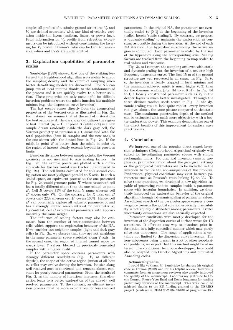
Fig. 3a to f compare the sampling achieved with staticand dynamic scaling for the inversion of a realistic highfrequency dispersion curve. The first 15 m of the groundstructure are well recovered in all cases. In Fig. 3a toc, the inversion is clearly trapped in local minima andthe minimum achieved misfit is much higher (0.2) thanfor the dynamic scaling (Fig. 3d to e, 0.01). In Fig. 3dto f, a loosely constrained parameter such as Vs in thedeeper layers is much better investigated. Through thethree distinct random seeds tested in Fig. 3, the dy-namic scaling results look quite robust: every inversionrun gives almost the same picture compared to the staticcase. The maximum penetration depth of the methodcan be estimated with much more objectivity with a bet-ter exploration power. This example demonstrates one ofthe direct benefits of this improvement for surface wavepractitioners.

4. Conclusion

We improved one of the popular direct search inver-sion techniques (Neighborhood Algorithm) originaly wellsuited for investigating parameter spaces with simplerectangular limits. For practical inversion cases in geo-physics, prior information about the geological settingsor the geophysical parameters are to be included in theinversion to reduce the non-uniqueness of the problem.Futhermore, physical conditions may exist between pa-rameters such as Poisson’s ratio linking Vp to Vs. Tosolve these questions, we developed a new algorithm ca-pable of generating random samples inside a parameterspace with irregular boundaries. In addition, we dras-ticaly improved the exploration behavior of the originalalgorithm through a dynamic scaling of parameter values.An efficient search of the parameter space ensures a con-vergence towards the global solution especially if sensibil-ity is not equally distributed among parameters. Betteruncertainty estimations are also naturally expected.

Parameter conditions were mostly developed for theinversion of the dispersion curves of surface waves for 1Dstructures. It offers an easy way to introduce prior in-formation in a fully controlled manner which may partlysolve non-uniqueness. The range of applications is cer-tainly not limited to the dispersion curve inversion. Thenon-uniqueness being present in a lot of other geophysi-cal problems, we expect that this method might be of in-terest. The conditional technique developped here couldalso be adapted into Genetic Algorithms and SimulatedAnnealing codes.

Acknowledgments.I would like to thank M. Sambridge for sharing his original

code in Fortran (2002) and for his helpful review. Interestingcomments from an anonymous reviewer also greatly improvedthe quality of the manuscript. I address my gratitude to Ce-cile Cornou, Pierre-Yves Bard and Denis Jongmans for readingpreliminary versions of the manuscript. This work could beachieved thanks to the EU funding granted to the NERIESproject (contract n RII3-CT-2006-026130 of programme I3 -

X - 4 WATHELET: PARAMETER CONDITIONS AND DYNAMIC SCALING

Integrated Infrastructure Initiative). The complete code de-scribed herein is available at http://www.geopsy.org under aGPL license.

References

A. W. F. Edwards. Likelihood, expanded edition. John Hop-kins, 1992.

R. B. Herrmann. Computer programs in seismology, vol IV,St Louis University, 1994.

Julian Ivanov, Richard D. Miller, Jianghai Xia, Don Steeples,and Choon B. Park. Joint analysis of refractions with sur-face waves: An inverse solution to the refraction-traveltimeproblem. Geophysics, 71:R131–R138, 2006.

A. J. Lomax and R. Snieder. Finding sets of acceptable solu-tions with a genetic algorithm with application to surfacewave group dispersion in Europe. Geophysical ResearchLetters, 21(24):2617–2620, 1994.

G. Nolet. Linearized inversion of (teleseismic) data. InR. Cassinis (ed.), editor, The solution of the inverse prob-lem in geophysical interpretation, pages 9–37. PlenumPress, 1981.

M. Picozzi, S. Parolai, and S. M. Richwalski. Joint inversionof H/V ratios and dispersion curves from seismic noise:Estimating the S-wave velocity of bedrock. GeophysicalResearch Letters, 32:L11308, doi:10.1029/2005GL022878,2005.

P. Rickwood and M. Sambridge. Efficient parallel inversionusing the Neighbourhood Algorithm. Geochemistry Geo-physics Geosystems, 7:doi:10.1029/2006GC001246, 2006.

N. Ryden and C.B. Park. Surface waves in inversely dispersivemedia. Near Surface Geophysics, 2:187–197, 2004.

M. Sambridge. Geophysical inversion with a neighbourhoodalgorithm: I. Searching a parameter space. Geophys. J.Int., 138:479–494, 1999.

F. Scherbaum, K.-G. Hinzen, and M. Ohrnberger. Deter-mination of shallow shear wave velocity profiles in theCologne/Germany area using ambient vibrations. Geophys.J. Int., 152:597–612, 2003.

M. K. Sen and P. L. Stoffa. Nonlinear one-dimensional seismicwaveform inversion using simulated annealing. Geophysics,56:1624–1638, 1991.

A. Tarantola. Inverse Problem Theory. Elsevier, Amsterdam,1987.

M. Wathelet. Array recordings of ambient vibrations: surface-wave inversion. PhD thesis, Universite de Liege, Belgium,2005.

M. Wathelet, D. Jongmans, and M. Ohrnberger. Surface waveinversion using a direct search algorithm and its applicationto ambient vibration measurements. Near Surface Geo-physics, 2:211–221, 2004.

M. Wathelet, LGIT, IRD, CNRS, Universit Joseph Fourier,Grenoble, France BP 53, 38041 Grenoble Cedex 9, France.(marc.wathelet@ujf-grenoble.fr)

Figure 1. A uniform random walk restricted to aVoronoi cell and by complex boundaries (modified afterSambridge [1999], Fig. 3). Starting from a sample insidethe cell (A), a Markov-Chain random walk is achievedby introducing random perturbations along all axes suc-cessively. Each random perturbation (for instance alongaxis i) is bounded by the rectangular boundary (li andui), by the limits of the Voronoi cells (xj and xl) and bythe intersection of axis i passing by A with the complexboundary (xb). Asymptotically the samples produced bythese walks are uniformly distributed inside the cell re-gardless of its shape (Sambridge [1999]). The light grayedarea is the region outside the parameter space still insidethe rectangular boundary.

WATHELET: PARAMETER CONDITIONS AND DYNAMIC SCALING X - 5

Figure 2. Effects of the axis scaling on cell connectivityfor a 2D Voronoi geometry. In Fig. a, the two axes havethe same scale (from -0.5 to 0.5). The light gray andthe dark gray cells are neighbors. In Fig. b, X axis isscaled by a factor 10 (from -0.05 to 0.05). The two cellsare not neighbors any longer. The dotted lines depict themodified Voronoi geometry after the addition of a pointB (or B′) at the limit of the cell centered around pointA.

0

10

20Depth (m)

0 1000 2000

Vs (m/s)

0

10

20Depth (m)

0 1000 2000

Vs (m/s)

0 1000 2000

Vs (m/s)

Misfit0.010 0.024 0.057 0.136 0.500

(a) (b) (c)

(d) (e) (f)

Figure 3. Effects of the parameter scaling on the searchcapabilities. The same high frequency dispersion curve(from 10 to 40 Hz) is inverted with the same parameter-ization (4 layers, 11 variable parameters). In all cases,10050 samples are generated by a NA sampler (200 it-erations with ns and nr set to 50). All Vs profiles witha misfit less than 1 are systematically shown. In Fig. ato c, the parameter space is scaled only at the begin-ning of the inversion process (static scaling, see text). InFig. d to f, it is continuously scaled after each iteration(dynamic scaling, see text). Inside each group, three dis-tinct seeds are randomly chosen to check the robustnessof the results. The black curve is the true Vs profile.