aa241x problem set 2 report team chimera - stanford …web.stanford.edu/~rsur/chimera...
TRANSCRIPT
Team Chimera – PS2
Page 1 of 79
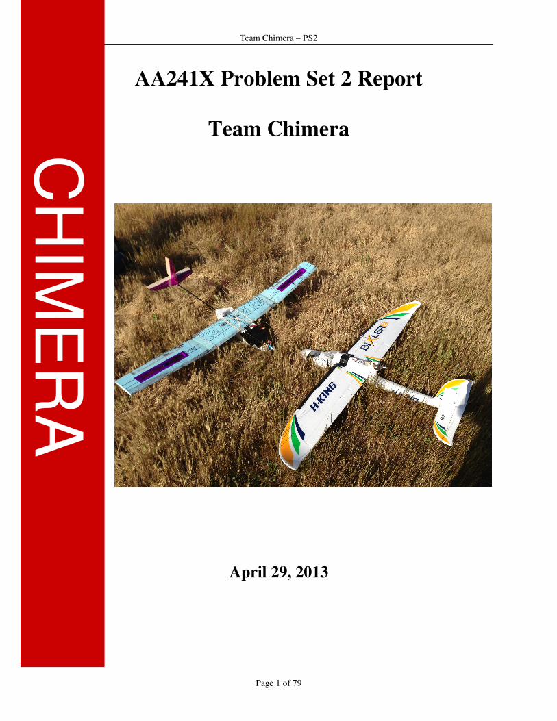
AA241X Problem Set 2 Report
Team Chimera
April 29, 2013
CH
IME
RA
Team Chimera – PS2
Page 2 of 79
Table of Contents
Listing of Tables ___________________________________________________ 3
Task 1: Experimental Determination of Trims for Bixler 2 _________________ 6
Task 2: Identification of Aircraft System Parameters _____________________ 9
Bixler 2 ________________________________________________________ 9
Chimera 1 and 2 ________________________________________________ 18
Task 3: Updated Mission Plan and Strategy ____________________________ 27
Task 4: Construction and Flight Testing of Chimera 1 ___________________ 31
Design and Construction of Chimera 1 _____________________________ 31
Construction Highlights for the Chimera 1 __________________________ 33
Aerodynamic Performance Estimations ____________________________ 39
Notes from RC Flight Testing & Considerations for Future Design
Iterations ______________________________________________________ 40
Task 5: Closing Control Loops ______________________________________ 42
Appendix A: Flight Data for Autonomous Flight (Day 1) _________________ 55
Appendix B: Flight Data for Autonomous Flight (Day 2) _________________ 65
Team Chimera – PS2
Page 3 of 79
Listing of Tables
Table 1: Mass estimation for Bixler 2. ____________________________________________ 11
Table 2: Inertia estimates for Bixler 2. ____________________________________________ 11
Table 3: Flight dynamics of the Bixler 2. __________________________________________ 14
Table 4: Stability analysis of aileron and rudder gains. ______________________________ 15
Table 5: Stability derivatives for Bixler 2. _________________________________________ 17
Table 6: Weight estimation for the Chimera 1 and Chimera 2__________________________ 20
Table 7: Interia estimates for the Chimera 1 and Chimera 2 ___________________________ 20
Table 8: Flight dynamics of Chimera 1. ___________________________________________ 24
Table 9: Stability analysis of rudder gains. ________________________________________ 25
Table 10: Stability analysis of aileron gains. _______________________________________ 25
Table 11: Stability derivatives for Chimera 1. ______________________________________ 26
Listing of Figures
Figure 1: Variation of airspeed during a sample autopilot run. _________________________ 6
Figure 2: Variation of deflection angles at different airspeeds. __________________________ 7
Figure 3: Variation of the throttle setting at different airspeeds._________________________ 8
Figure 4: Aerodynamic model of the Bixler 2 (isometric view).__________________________ 9
Figure 5: Aerodynamic model of the Bixler 2 (top view). _____________________________ 10
Figure 6: Lift coefficient vs. angle of attack for Bixler 2. ______________________________ 12
Figure 7: Drag polar for Bixler 2. _______________________________________________ 12
Figure 8: CL/CD vs. angle of attack for Bixler 2. ____________________________________ 13
Figure 9: Longitudinal modes for Bixler 2. ________________________________________ 13
Figure 10: Lateral modes for Bixler 2. ____________________________________________ 14
Figure 11: Flight dynamics of Bixler 2. ___________________________________________ 15
Figure 12: Analysis images, distributed point mass is added along the body axis to account for
the fuselage. ________________________________________________________________ 16
Figure 13: Chimera 1 aerodynamic model (isometric view). ___________________________ 18
Figure 14: Chimera 1 aerodynamic model (top view). ________________________________ 18
Figure 15: Design of the Chimera 2 (isometric view). ________________________________ 19
Figure 16: Design of the Chimera 2 (top and front views). ____________________________ 19
Figure 17: CL vs. alpha for Chimera 1. ___________________________________________ 21
Figure 18: Drag polar for Chimera 1. ____________________________________________ 22
Figure 19: CL/CD vs. alpha for Chimera 1. ________________________________________ 22
Figure 20: Longitudinal modes for Chimera 1. _____________________________________ 23
Team Chimera – PS2
Page 4 of 79
Figure 21: Lateral modes for Chimera 1. __________________________________________ 23
Figure 22: Flight dynamics of Chimera 1. _________________________________________ 24
Figure 23: Analysis images for the Chimera 1. _____________________________________ 25
Figure 24: Sample run 1 of the simulation. The plane starts at the outside of the field. In this run,
the score was 25. The time it took to find all three beacons was 78 seconds. The sum of the norms
of the estimation errors was 11.6 meters. Large blue circle: field; green circles: Field of View
when snapshot was taken; magenta circles: location of the plane; red circles: target position
estimate returned by snapshot; blue dots: estimates of the locations of the beacons; blue
asterisks (not easily visible, as they are covered by other lines): beacon locations. _________ 27
Figure 25: Sample run 2 of the simulation. The plane starts at the outside of the field. In this run,
the score was 33. The time it took to find all three beacons was 160 seconds. The sum of the
norms of the estimation errors was 9 meters (the minimum achievable value). Large blue circle:
field; green circles: Field of View when snapshot was taken; magenta circles: location of the
plane; red circles: target position estimate returned by snapshot; blue dots: estimates of the
locations of the beacons; blue asterisks (not easily visible, as they are covered by other lines):
beacon locations. ____________________________________________________________ 28
Figure 26: Score distribution for all simulations. Average score: 29.64. Standard Deviation:
4.83._______________________________________________________________________ 29
Figure 27: Time to find all beacons for all simulations. Average time: 162 seconds. Standard
Deviation: 83 seconds. ________________________________________________________ 29
Figure 28: Sum of the norms of the estimation errors. Average value of the sum: 10.5 meters.
Standard Deviation: 2.31 meters. ________________________________________________ 30
Figure 29: Chimera 1 assembled and ready to fly. Motor mount allows airflow to cool onboard
electronics and rubber band-secured wing provides easy access to flight hardware. ________ 31
Figure 30: The foam tail mount is designed for easy assembly, but made the tail less torsionally
rigid. ______________________________________________________________________ 33
Figure 31: First generation avionics chassis. ______________________________________ 34
Figure 32: Foam cutting of the two dihedral sections. ________________________________ 34
Figure 33: Vacuum bagging the five wing pieces. ___________________________________ 35
Figure 34: Cured wing pieces (after much sanding). _________________________________ 36
Figure 35: Alignment and curing set-up for joining wing segments. _____________________ 36
Figure 36: Joined wing piece. __________________________________________________ 37
Figure 37: Milling slots for servo installation. ______________________________________ 37
Figure 38: Fixturing for wing machining. _________________________________________ 38
Figure 39: Cutting the external shape of the fuselage. ________________________________ 38
Figure 40: Milling the internal cavity of the fuselage. ________________________________ 39
Figure 41: Chimera 1 on its virgin flight! _________________________________________ 41
Figure 42: Root locus of the pitch rate loop. _______________________________________ 43
Figure 43: Negative root locus of the pitch rate loop. ________________________________ 44
Figure 44: Block diagram of the pitch control loop. _________________________________ 45

Team Chimera – PS2
Page 5 of 79
Figure 45: Block diagram of altitude hold control. __________________________________ 45
Figure 46: Simulink model for pitch control loop. ___________________________________ 46
Figure 47: Output of theta for a reference command of 26.25°. ________________________ 46
Figure 48: Simulink model for altitude control loop. _________________________________ 47
Figure 49: Output of altitude holding for a reference command to descend 3 meters. _______ 47
Figure 50: Block diagram of airspeed hold. ________________________________________ 48
Figure 51: Block diagram of the roll control loop. __________________________________ 49
Figure 52: Block diagram of the yaw loop. ________________________________________ 49
Figure 53: Block diagram of the sideslip loop. _____________________________________ 50
Figure 54: Simulink model for the roll control loop. _________________________________ 50
Figure 55: Simulink response of bank angle for reference command of 60° (alternating every 5
seconds). ___________________________________________________________________ 51
Figure 56: Simulink model for yaw loop. __________________________________________ 51
Figure 57: Simulink response of yaw angle for a refrence command of 30° (alternating every 25
seconds). ___________________________________________________________________ 52
Figure 58: First autopilot trial __________________________________________________ 52
Figure 59: Second autopilot trial. _______________________________________________ 53
Figure 60: Third autopilot trial. _________________________________________________ 53

Team Chimera – PS2
Page 6 of 79
Task 1: Experimental Determination of Trims for Bixler 2 Primary contributors: Ritobrata Sur, Manuel Lopez, and Jack Tsai
The trim settings for the Bixler 2 were experimentally determined from the autopilot portions of
the flight where it held a straight course across Lake Lagunita at relatively uniform airspeed. A
sample plot of airspeed measurements from one of the autopilot sections is show below.
604 606 608 610 612 614 61613
14
15
16
17
18
19
20
Time [s]
Air
spee
d [
m/s
]
Figure 1: Variation of airspeed during a sample autopilot run.
Clearly it can be seen that the airspeed had a significant variation during this process and would
lead to significant uncertainties in these measurements. The mean deflection in the servo angles
were estimated from the log files of the Ardupilot. A large error (standard deviation of about
40% in some cases) in these measurements indicates that these obtained values are only valid up
to an order of magnitude.
Team Chimera – PS2
Page 7 of 79
6 8 10 12 14 16 18
-5
0
5
Aileron Elevator Rudder
Trim
angle
s [d
egre
es]
Air speed [m/s]
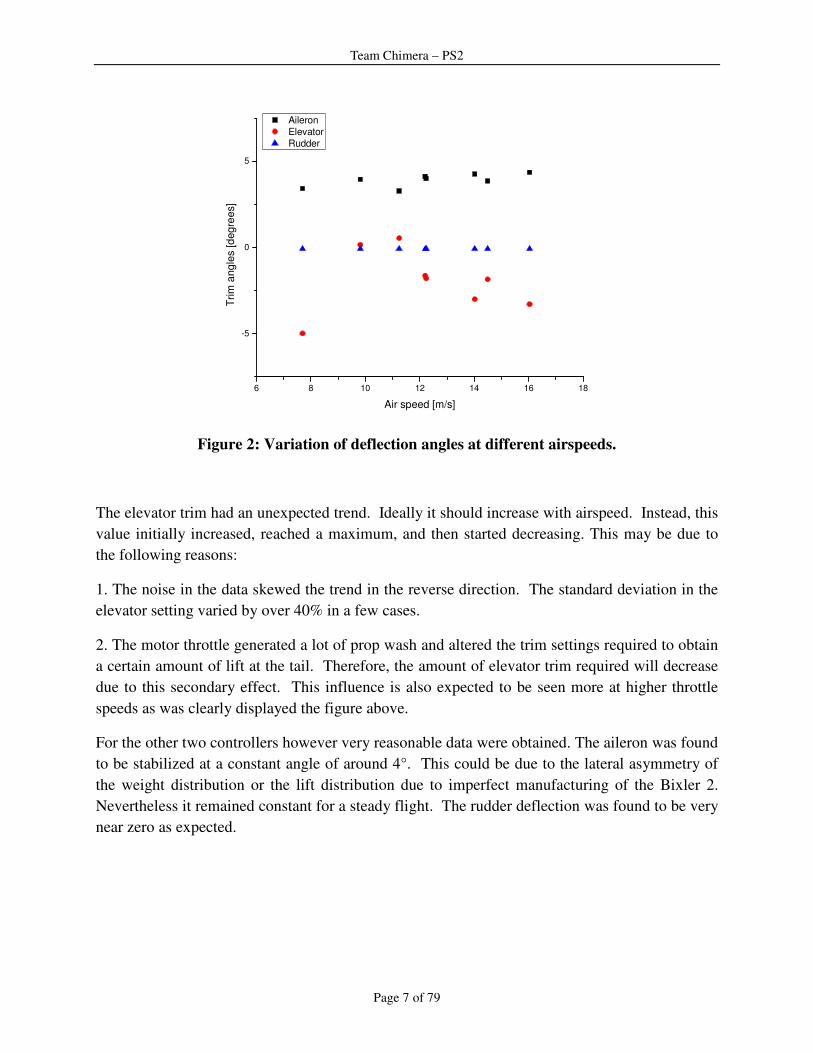
Figure 2: Variation of deflection angles at different airspeeds.
The elevator trim had an unexpected trend. Ideally it should increase with airspeed. Instead, this
value initially increased, reached a maximum, and then started decreasing. This may be due to
the following reasons:
1. The noise in the data skewed the trend in the reverse direction. The standard deviation in the
elevator setting varied by over 40% in a few cases.
2. The motor throttle generated a lot of prop wash and altered the trim settings required to obtain
a certain amount of lift at the tail. Therefore, the amount of elevator trim required will decrease
due to this secondary effect. This influence is also expected to be seen more at higher throttle
speeds as was clearly displayed the figure above.
For the other two controllers however very reasonable data were obtained. The aileron was found
to be stabilized at a constant angle of around 4°. This could be due to the lateral asymmetry of
the weight distribution or the lift distribution due to imperfect manufacturing of the Bixler 2.
Nevertheless it remained constant for a steady flight. The rudder deflection was found to be very
near zero as expected.

Team Chimera – PS2
Page 8 of 79
6 8 10 12 14 16 18
40
50
60
70
80
Th
rottle
settin
g [%
]
Air speed [m/s]
Figure 3: Variation of the throttle setting at different airspeeds.
The variation in the throttle settings followed a near to linear trend as expected. The first point
was close to stalling and hence may be ignored.
According to these measurements we can conclude that the following order may be followed for
a stable flight. First, the throttle setting must be fixed, then followed by the elevator. The
ailerons must be maintained at the trim settings when holding course. These settings may be
changed as and when necessary to balance the effects of wind, etc. The rudder may be the final
knob that we can change to fine tune the plane's orientation.

Team Chimera – PS2
Page 9 of 79
Task 2: Identification of Aircraft System Parameters Primary contributor: Hao Dong and Marcel Nations
Bixler 2
1. Aerodynamic Modeling of Bixler2 in XFLR5
The Bixler 2 was modeled and analyzed using the XFLR5 software package. AVL and Vlaero
were also considered as analysis tools, but XFLR5 was selected as the most straightforward one
to use. Based on measured geometry from the Bixler 2, MM 300 was selected as the most
similar airfoil for analysis. The horizontal and vertical tail are modeled as NACA 0006 airfoils.
The wing, vertical tail (VT), and horizontal tail (HT) were modeled as trapezoidal sections. Each
section of the wing was defined by the root and tip chord, dihedral, and offset based on
measurements of the Bixler 2. Aileron, rudder, elevator are also defined according to measured
dimensions.
Figure 4: Aerodynamic model of the Bixler 2 (isometric view).

Team Chimera – PS2
Page 10 of 79
Figure 5: Aerodynamic model of the Bixler 2 (top view).
2. Weight and Inertia Estimates
Weight and inertia estimation is very important for properly trimming the controls of an aircraft.
Without a proper estimation of these parameters, the stability derivatives cannot be accurately
calculated. In the case of the Bixler 2, it was possible to measure each component separately
using a digital balance. The propulsion hardware and avionics were then treated as point masses
in XFLR5.

Team Chimera – PS2
Page 11 of 79
Table 1: Mass estimation for Bixler 2. Table 2: Inertia estimates for Bixler 2.
Mass Estimation (g)
Wing 250
Fuselage VT&HT 150
Propulsion 156
Motor 24
Propeller 18
Battery 118
Avionics 209
GPS 17
Pitot Tube 11
Servos (QTY. 4) 36
Transmitter 11
Autopilot
Transmitter 17
Votage Regulator 21
Autopilot Board 28
Speed Controller 38
Wiring 30
Total Mass (g) 765
3. Aerodynamic Performance Analysis
The analysis was performed in XFLR5. The XFLR5 analysis combines a three-dimensional
panel method and a vortex lattice method (VLM). Although VLM usually neglects viscosity,
XFLR5 has the viscous analysis function which interpolates from the airfoil analysis in 2D
viscous flow. The Reynolds number of the analysis ranges from 80,000 to 210,000 which
corresponds to a velocity of 6 to 15 m/s. The CL curve is treated as independent of velocity.
XFLR5 cannot interpolate beyond an angle of attack of 11.3 ; this indicates a stall angle of 11.3 .
The following diagrams plot CL as a function of angle of attack, the CL/CD polar, and CL/CD
versus angle of attack at different velocities.
Dimensions
Mass 765 g
Wing area 0.25 m^2
Wing span 1.48 m
HT area 0.05 m^2
VT area 0.02 m^2
X_CoG 0.085 m
Y_CoG 0
Z_CoG - 0.03
-
Ixx 0.028 kg-m2
Iyy 0.026 kg-m2
Izz 0.053 kg-m2
Ixz 0

Team Chimera – PS2
Page 12 of 79
Figure 6: Lift coefficient vs. angle of attack for Bixler 2.
Figure 7: Drag polar for Bixler 2.

Team Chimera – PS2
Page 13 of 79
Figure 8: CL/CD vs. angle of attack for Bixler 2.
4. Stability Analysis
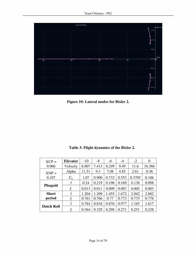
The stability analysis is performed in XFLR5. The following diagrams show the eigenvalues of
longitudinal and lateral modes as a function of velocity (from 6.8 m/s to 16.4 m/s corresponding
to elevator angles of -10 to 0 ). The two longitudinal modes and dutch roll mode are
underdamped. The Spiral mode and rolling mode are overdamped.
Figure 9: Longitudinal modes for Bixler 2.
Team Chimera – PS2
Page 14 of 79
Figure 10: Lateral modes for Bixler 2.
Table 3: Flight dynamics of the Bixler 2.
XCP =
0.066
Elevator -10 -8 -6 -4 -2 0
Velocity 6.807 7.413 8.249 9.49 11.6 16.366
XNP =
0.107
Alpha 11.51 9.3 7.08 4.85 2.61 0.36
CL 1.07 0.906 0.732 0.553 0.3705 0.186
Phugoid f 0.24 0.219 0.196 0.169 0.138 0.098
� 0.013 0.011 0.009 0.007 0.005 0.003
Short
period f 1.204 1.309 1.455 1.672 2.042 2.882
� 0.761 0.766 0.77 0.773 0.775 0.776
Dutch Roll f 0.784 0.818 0.876 0.977 1.165 1.617
� 0.364 0.329 0.298 0.271 0.251 0.238
Team Chimera – PS2
Page 15 of 79
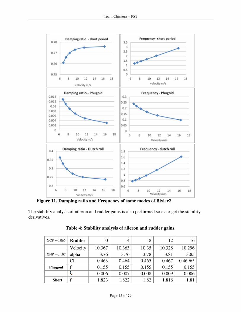
Figure 11. Damping ratio and Frequency of some modes of Bixler2
The stability analysis of aileron and rudder gains is also performed so as to get the stability
derivatives.
Table 4: Stability analysis of aileron and rudder gains.
XCP = 0.066 Rudder 0 4 8 12 16
Velocity 10.367 10.363 10.35 10.328 10.296
XNP = 0.107 alpha 3.76 3.76 3.78 3.81 3.85
Cl 0.463 0.464 0.465 0.467 0.46965
Phugoid f 0.155 0.155 0.155 0.155 0.155
0.006 0.007 0.008 0.009 0.006
Short f 1.823 1.822 1.82 1.816 1.81
Team Chimera – PS2
Page 16 of 79
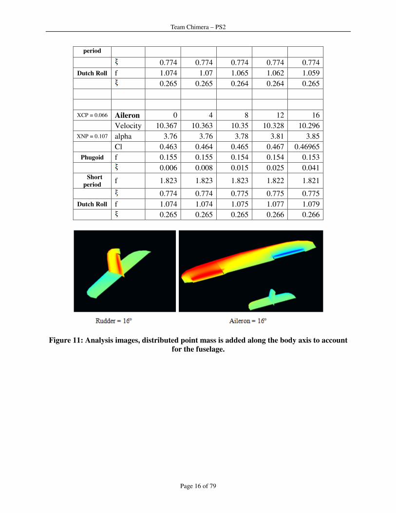
period
0.774 0.774 0.774 0.774 0.774
Dutch Roll f 1.074 1.07 1.065 1.062 1.059
0.265 0.265 0.264 0.264 0.265
XCP = 0.066 Aileron 0 4 8 12 16
Velocity 10.367 10.363 10.35 10.328 10.296
XNP = 0.107 alpha 3.76 3.76 3.78 3.81 3.85
Cl 0.463 0.464 0.465 0.467 0.46965
Phugoid f 0.155 0.155 0.154 0.154 0.153
0.006 0.008 0.015 0.025 0.041
Short
period f 1.823 1.823 1.823 1.822 1.821
0.774 0.774 0.775 0.775 0.775
Dutch Roll f 1.074 1.074 1.075 1.077 1.079
0.265 0.265 0.265 0.266 0.266
Figure 11: Analysis images, distributed point mass is added along the body axis to account
for the fuselage.

Team Chimera – PS2
Page 17 of 79
5. Stability Derivatives
The stability derivatives for trim conditions in responses to changes of elevator angle are shown
below.
Table 5: Stability derivatives for Bixler 2.
Velocity
(m/s) 6.8070 7.4130 8.2490 9.4900 11.6000 16.3660
Elevator
-
10.0000 -8.0000 -6.0000 -4.0000 -2.0000 0.0000
Cla 4.8343 4.9479 5.0436 5.1199 5.1757 5.2101
CLq 9.4416 9.5599 9.6573 9.7327 9.7853 9.8146
Cma -1.4639 -1.4688 -1.4730 -1.4766 -1.4797 -1.4821
Cmq
-
16.6345
-
16.8134
-
16.9630
-
17.0822
-
17.1703
-
17.2268
CYb -0.2545 -0.2554 -0.2561 -0.2563 -0.2562 -0.2556
Cyp 0.0642 0.0443 0.0243 0.0044 -0.0153 -0.0347
CYr 0.2332 0.2347 0.2348 0.2333 0.2303 0.2256
Clb -0.0701 -0.0660 -0.0620 -0.0582 -0.0545 -0.0510
Clp -0.4906 -0.4930 -0.4949 -0.4963 -0.4974 -0.4980
Clr 0.2556 0.2161 0.1762 0.1361 0.0958 0.0555
Cnb 0.0866 0.0881 0.0898 0.0919 0.0943 0.0969
Cnp -0.1863 -0.1594 -0.1320 -0.1040 -0.0756 -0.0469
Cnr -0.0800 -0.0832 -0.0861 -0.0886 -0.0907 -0.0923
Cxe -0.0374 -0.0312 -0.0247 -0.0181 -0.0114 -0.0046
CYe 0.0000 0.0000 0.0000 0.0000 0.0000 0.0000
Cze -0.5271 -0.5305 -0.5332 -0.5351 -0.5362 -0.5365
CLe 0.0000 0.0000 0.0000 0.0000 0.0000 0.0000
Cme -1.6279 -1.6382 -1.6468 -1.6538 -1.6591 -1.6627
CNe 0.0000 0.0000 0.0000 0.0000 0.0000 0.0000
Team Chimera – PS2
Page 18 of 79
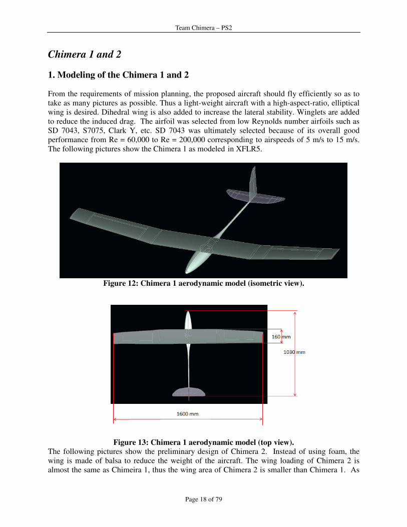
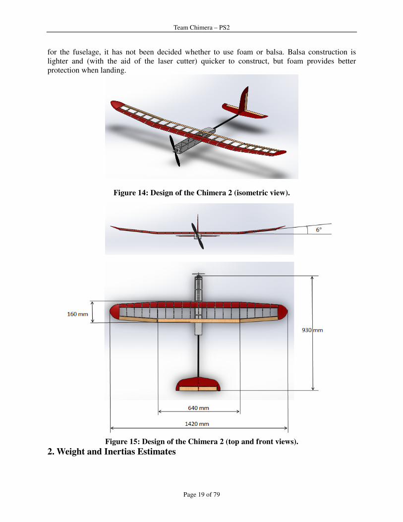
Chimera 1 and 2
1. Modeling of the Chimera 1 and 2
From the requirements of mission planning, the proposed aircraft should fly efficiently so as to
take as many pictures as possible. Thus a light-weight aircraft with a high-aspect-ratio, elliptical
wing is desired. Dihedral wing is also added to increase the lateral stability. Winglets are added
to reduce the induced drag. The airfoil was selected from low Reynolds number airfoils such as
SD 7043, S7075, Clark Y, etc. SD 7043 was ultimately selected because of its overall good
performance from Re = 60,000 to Re = 200,000 corresponding to airspeeds of 5 m/s to 15 m/s.
The following pictures show the Chimera 1 as modeled in XFLR5.
Figure 12: Chimera 1 aerodynamic model (isometric view).
Figure 13: Chimera 1 aerodynamic model (top view).
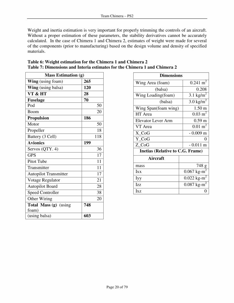
The following pictures show the preliminary design of Chimera 2. Instead of using foam, the
wing is made of balsa to reduce the weight of the aircraft. The wing loading of Chimera 2 is
almost the same as Chimeira 1, thus the wing area of Chimera 2 is smaller than Chimera 1. As
Team Chimera – PS2
Page 19 of 79
for the fuselage, it has not been decided whether to use foam or balsa. Balsa construction is
lighter and (with the aid of the laser cutter) quicker to construct, but foam provides better
protection when landing.
Figure 14: Design of the Chimera 2 (isometric view).
Figure 15: Design of the Chimera 2 (top and front views).
2. Weight and Inertias Estimates
Team Chimera – PS2
Page 20 of 79
Weight and inertia estimation is very important for properly trimming the controls of an aircraft.
Without a proper estimation of these parameters, the stability derivatives cannot be accurately
calculated. In the case of Chimera 1 and Chimera 2, estimates of weight were made for several
of the components (prior to manufacturing) based on the design volume and density of specified
materials.
Table 6: Weight estimation for the Chimera 1 and Chimera 2
Table 7: Dimensions and Interia estimates for the Chimera 1 and Chimera 2
Mass Estimation (g)
Wing (using foam) 265
Wing (using balsa) 120
VT & HT 28
Fuselage 70
Pod 50
Boom 20
Propulsion 186
Motor 50
Propeller 18
Battery (3 Cell) 118
Avionics 199
Servos (QTY. 4) 36
GPS 17
Pitot Tube 11
Transmitter 11
Autopilot Transmitter 17
Votage Regulator 21
Autopilot Board 28
Speed Controller 38
Other Wiring 20
Total Mass (g) (using
foam) 748
(using balsa) 603
Dimensions
Wing Area (foam) 0.241 m2
(balsa) 0.208
Wing Loading(foam) 3.1 kg/m2
(balsa) 3.0 kg/m2
Wing Span(foam wing) 1.50 m
HT Area 0.03 m2
Elevator Lever Arm 0.59 m
VT Area 0.01 m2
X_CoG - 0.009 m
Y_CoG 0
Z_CoG - 0.011 m
Inetias (Relative to C.G. Frame)
Aircraft
mass 748 g
Ixx 0.067 kg-m2
Iyy 0.022 kg-m2
Izz 0.087 kg-m2
Ixz 0
Team Chimera – PS2
Page 21 of 79
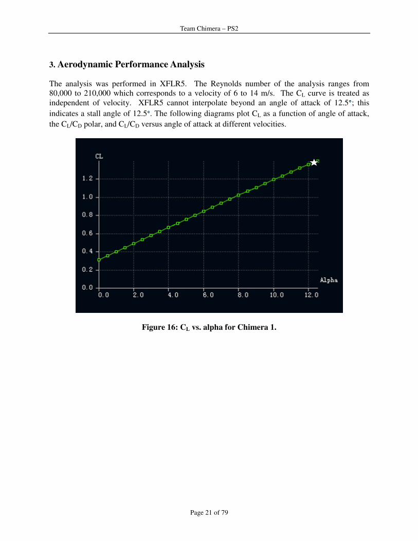
3. Aerodynamic Performance Analysis
The analysis was performed in XFLR5. The Reynolds number of the analysis ranges from
80,000 to 210,000 which corresponds to a velocity of 6 to 14 m/s. The CL curve is treated as
independent of velocity. XFLR5 cannot interpolate beyond an angle of attack of 12.5 ; this
indicates a stall angle of 12.5 . The following diagrams plot CL as a function of angle of attack,
the CL/CD polar, and CL/CD versus angle of attack at different velocities.
Figure 16: CL vs. alpha for Chimera 1.

Team Chimera – PS2
Page 22 of 79
Figure 17: Drag polar for Chimera 1.
Figure 18: CL/CD vs. alpha for Chimera 1.
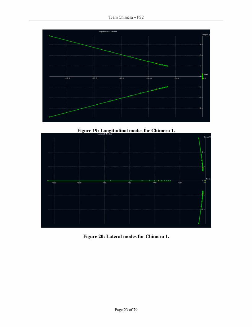
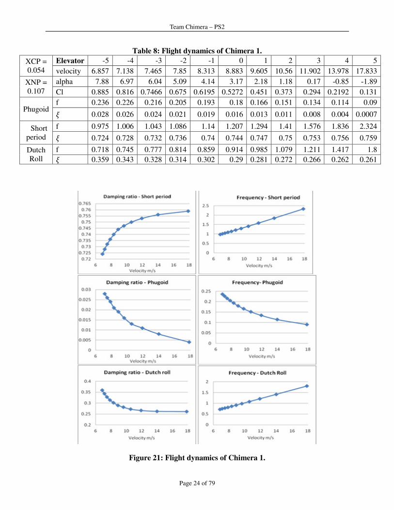
4. Stability Analysis
The stability analysis is performed in XFLR5. The following diagrams show the eigenvalues of
longitudinal and lateral modes as a function of velocity (from 6.8 m/s to 16.4m/s corresponding
to elevator angles of -10 to 0 ). The two longitudinal modes and dutch roll mode are
underdamped. The Spiral mode and rolling mode are overdamped.
Team Chimera – PS2
Page 23 of 79
Figure 19: Longitudinal modes for Chimera 1.
Figure 20: Lateral modes for Chimera 1.
Team Chimera – PS2
Page 24 of 79
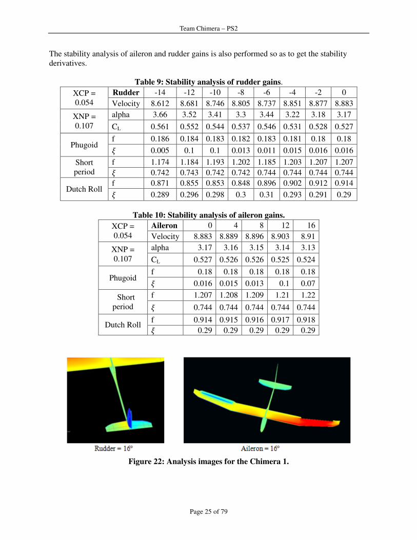
Table 8: Flight dynamics of Chimera 1.
XCP =
0.054
Elevator -5 -4 -3 -2 -1 0 1 2 3 4 5
velocity 6.857 7.138 7.465 7.85 8.313 8.883 9.605 10.56 11.902 13.978 17.833
XNP =
0.107
alpha 7.88 6.97 6.04 5.09 4.14 3.17 2.18 1.18 0.17 -0.85 -1.89
Cl 0.885 0.816 0.7466 0.675 0.6195 0.5272 0.451 0.373 0.294 0.2192 0.131
Phugoid f 0.236 0.226 0.216 0.205 0.193 0.18 0.166 0.151 0.134 0.114 0.09
� 0.028 0.026 0.024 0.021 0.019 0.016 0.013 0.011 0.008 0.004 0.0007
Short
period
f 0.975 1.006 1.043 1.086 1.14 1.207 1.294 1.41 1.576 1.836 2.324
� 0.724 0.728 0.732 0.736 0.74 0.744 0.747 0.75 0.753 0.756 0.759
Dutch
Roll
f 0.718 0.745 0.777 0.814 0.859 0.914 0.985 1.079 1.211 1.417 1.8
� 0.359 0.343 0.328 0.314 0.302 0.29 0.281 0.272 0.266 0.262 0.261
Figure 21: Flight dynamics of Chimera 1.
Team Chimera – PS2
Page 25 of 79
The stability analysis of aileron and rudder gains is also performed so as to get the stability
derivatives.
Table 9: Stability analysis of rudder gains.
XCP =
0.054
Rudder -14 -12 -10 -8 -6 -4 -2 0
Velocity 8.612 8.681 8.746 8.805 8.737 8.851 8.877 8.883
XNP =
0.107
alpha 3.66 3.52 3.41 3.3 3.44 3.22 3.18 3.17
CL 0.561 0.552 0.544 0.537 0.546 0.531 0.528 0.527
Phugoid f 0.186 0.184 0.183 0.182 0.183 0.181 0.18 0.18
� 0.005 0.1 0.1 0.013 0.011 0.015 0.016 0.016
Short
period
f 1.174 1.184 1.193 1.202 1.185 1.203 1.207 1.207
� 0.742 0.743 0.742 0.742 0.744 0.744 0.744 0.744
Dutch Roll f 0.871 0.855 0.853 0.848 0.896 0.902 0.912 0.914
� 0.289 0.296 0.298 0.3 0.31 0.293 0.291 0.29
Table 10: Stability analysis of aileron gains.
XCP =
0.054
Aileron 0 4 8 12 16
Velocity 8.883 8.889 8.896 8.903 8.91
XNP =
0.107
alpha 3.17 3.16 3.15 3.14 3.13
CL 0.527 0.526 0.526 0.525 0.524
Phugoid f 0.18 0.18 0.18 0.18 0.18
� 0.016 0.015 0.013 0.1 0.07
Short
period
f 1.207 1.208 1.209 1.21 1.22
� 0.744 0.744 0.744 0.744 0.744
Dutch Roll f 0.914 0.915 0.916 0.917 0.918
� 0.29 0.29 0.29 0.29 0.29
Figure 22: Analysis images for the Chimera 1.
Team Chimera – PS2
Page 26 of 79
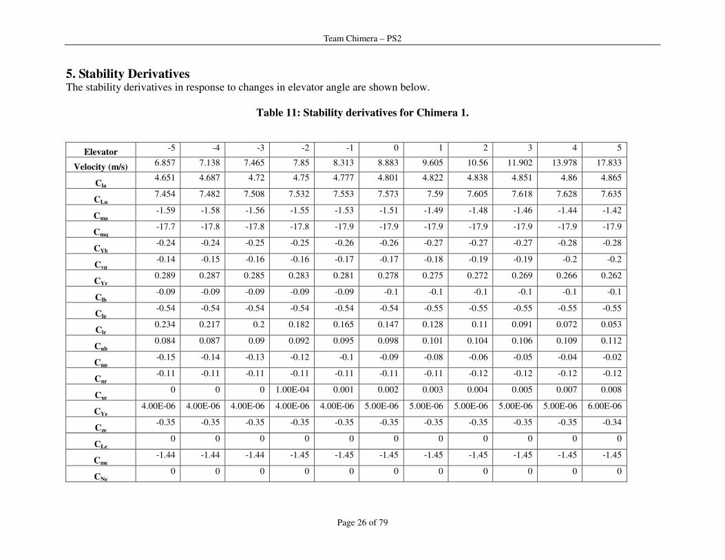
5. Stability Derivatives The stability derivatives in response to changes in elevator angle are shown below.
Table 11: Stability derivatives for Chimera 1.
Elevator -5 -4 -3 -2 -1 0 1 2 3 4 5
Velocity (m/s) 6.857 7.138 7.465 7.85 8.313 8.883 9.605 10.56 11.902 13.978 17.833
Cla 4.651 4.687 4.72 4.75 4.777 4.801 4.822 4.838 4.851 4.86 4.865
CLq 7.454 7.482 7.508 7.532 7.553 7.573 7.59 7.605 7.618 7.628 7.635
Cma -1.59 -1.58 -1.56 -1.55 -1.53 -1.51 -1.49 -1.48 -1.46 -1.44 -1.42
Cmq -17.7 -17.8 -17.8 -17.8 -17.9 -17.9 -17.9 -17.9 -17.9 -17.9 -17.9
CYb -0.24 -0.24 -0.25 -0.25 -0.26 -0.26 -0.27 -0.27 -0.27 -0.28 -0.28
Cyp -0.14 -0.15 -0.16 -0.16 -0.17 -0.17 -0.18 -0.19 -0.19 -0.2 -0.2
CYr 0.289 0.287 0.285 0.283 0.281 0.278 0.275 0.272 0.269 0.266 0.262
Clb -0.09 -0.09 -0.09 -0.09 -0.09 -0.1 -0.1 -0.1 -0.1 -0.1 -0.1
Clp -0.54 -0.54 -0.54 -0.54 -0.54 -0.54 -0.55 -0.55 -0.55 -0.55 -0.55
Clr 0.234 0.217 0.2 0.182 0.165 0.147 0.128 0.11 0.091 0.072 0.053
Cnb 0.084 0.087 0.09 0.092 0.095 0.098 0.101 0.104 0.106 0.109 0.112
Cnp -0.15 -0.14 -0.13 -0.12 -0.1 -0.09 -0.08 -0.06 -0.05 -0.04 -0.02
Cnr -0.11 -0.11 -0.11 -0.11 -0.11 -0.11 -0.11 -0.12 -0.12 -0.12 -0.12
Cxe 0 0 0 1.00E-04 0.001 0.002 0.003 0.004 0.005 0.007 0.008
CYe 4.00E-06 4.00E-06 4.00E-06 4.00E-06 4.00E-06 5.00E-06 5.00E-06 5.00E-06 5.00E-06 5.00E-06 6.00E-06
Cze -0.35 -0.35 -0.35 -0.35 -0.35 -0.35 -0.35 -0.35 -0.35 -0.35 -0.34
CLe 0 0 0 0 0 0 0 0 0 0 0
Cme -1.44 -1.44 -1.44 -1.45 -1.45 -1.45 -1.45 -1.45 -1.45 -1.45 -1.45
CNe 0 0 0 0 0 0 0 0 0 0 0
Team Chimera – PS2
Page 27 of 79
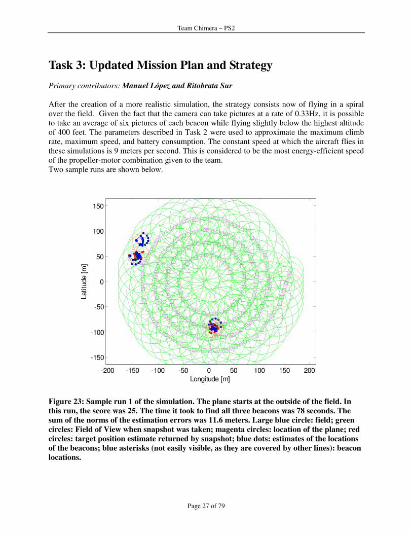
Task 3: Updated Mission Plan and Strategy
Primary contributors: Manuel López and Ritobrata Sur
After the creation of a more realistic simulation, the strategy consists now of flying in a spiral
over the field. Given the fact that the camera can take pictures at a rate of 0.33Hz, it is possible
to take an average of six pictures of each beacon while flying slightly below the highest altitude
of 400 feet. The parameters described in Task 2 were used to approximate the maximum climb
rate, maximum speed, and battery consumption. The constant speed at which the aircraft flies in
these simulations is 9 meters per second. This is considered to be the most energy-efficient speed
of the propeller-motor combination given to the team.
Two sample runs are shown below.
-200 -150 -100 -50 0 50 100 150 200
-150
-100
-50
0
50
100
150
Longitude [m]
Latitu
de [
m]
Figure 23: Sample run 1 of the simulation. The plane starts at the outside of the field. In
this run, the score was 25. The time it took to find all three beacons was 78 seconds. The
sum of the norms of the estimation errors was 11.6 meters. Large blue circle: field; green
circles: Field of View when snapshot was taken; magenta circles: location of the plane; red
circles: target position estimate returned by snapshot; blue dots: estimates of the locations
of the beacons; blue asterisks (not easily visible, as they are covered by other lines): beacon
locations.

Team Chimera – PS2
Page 28 of 79
In sample run 1, the strategy found all three beacons very quickly, but could not create a very
good estimate on the location of the beacons. Below is a sample run in which almost the
opposite happens: it takes a long time to find the beacons, but their location is estimated with
high accuracy.
-200 -150 -100 -50 0 50 100 150 200
-150
-100
-50
0
50
100
150
Longitude [m]
Latitu
de [
m]
Figure 24: Sample run 2 of the simulation. The plane starts at the outside of the field. In
this run, the score was 33. The time it took to find all three beacons was 160 seconds. The
sum of the norms of the estimation errors was 9 meters (the minimum achievable value).
Large blue circle: field; green circles: Field of View when snapshot was taken; magenta
circles: location of the plane; red circles: target position estimate returned by snapshot;
blue dots: estimates of the locations of the beacons; blue asterisks (not easily visible, as they
are covered by other lines): beacon locations.
To estimate the performance of the strategy, we ran the simulation 2,445 times. Below are the
results.
Team Chimera – PS2
Page 29 of 79
Figure 25: Score distribution for all simulations. Average score: 29.64. Standard
Deviation: 4.83.
Figure 26: Time to find all beacons for all simulations. Average time: 162 seconds.
Standard Deviation: 83 seconds.

Team Chimera – PS2
Page 30 of 79
Figure 27: Sum of the norms of the estimation errors. Average value of the sum: 10.5
meters. Standard Deviation: 2.31 meters.
It is important to note that the time it takes to find the beacons is more dependent on the
maximum speed of the aircraft than on any other factor. The accuracy of the estimated beacon
locations is on average fairly good, as the minimum value achievable here is 9 meters. Another
interesting observation is that the score hits a ceiling value of 33.5. This can be caused by the
fact that there is a ceiling in the accuracy with which we can estimate the location of the beacons
and a minimum amount of time necessary to find all beacons.
The simulation does not yet take into account the following:
1. The physics of the plane and the implemented control law
2. Constraints in the turning radius (with the strategy of flying in a spiral, the turning radius
is not so important in the simulation)
3. Constraints in the climb rate; the current model assumes the plane climbs at a constant
angle, which was measured during the test flights
4. Wind gusts
5. Accurate estimates of battery consumption; right now the simulation uses a drag
coefficient and the height to calculate the energy necessary to move the airplane. It would
be good to implement measurements of the real battery consumption in the simulation.
In conclusion, the simulations show that for a spiral flight, the accuracy with which the beacon
locations is estimated is very good, while the time it takes to find all of them depends strongly on
the speed of the aircraft. The next step in the devising of the strategy is to assess how beneficial
it would be to increase the speed of the aircraft. Even though higher speeds would help us attain
a higher score, the battery consumption limits would make it risky to try to fly the plane at high
but sub-optimal speeds.
Team Chimera – PS2
Page 31 of 79
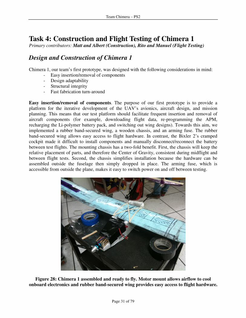
Task 4: Construction and Flight Testing of Chimera 1 Primary contributors: Matt and Albert (Construction), Rito and Manuel (Flight Testing)
Design and Construction of Chimera 1
Chimera 1, our team’s first prototype, was designed with the following considerations in mind:
- Easy insertion/removal of components
- Design adaptability
- Structural integrity
- Fast fabrication turn-around
Easy insertion/removal of components. The purpose of our first prototype is to provide a
platform for the iterative development of the UAV’s avionics, aircraft design, and mission
planning. This means that our test platform should facilitate frequent insertion and removal of
aircraft components (for example, downloading flight data, re-programming the APM,
recharging the Li-polymer battery pack, and switching out wing designs). Towards this aim, we
implemented a rubber band-secured wing, a wooden chassis, and an arming fuse. The rubber
band-secured wing allows easy access to flight hardware. In contrast, the Bixler 2’s cramped
cockpit made it difficult to install components and manually disconnect/reconnect the battery
between test flights. The mounting chassis has a two-fold benefit. First, the chassis will keep the
relative placement of parts, and therefore the Center of Gravity, consistent during midflight and
between flight tests. Second, the chassis simplifies installation because the hardware can be
assembled outside the fuselage then simply dropped in place. The arming fuse, which is
accessible from outside the plane, makes it easy to switch power on and off between testing.
Figure 28: Chimera 1 assembled and ready to fly. Motor mount allows airflow to cool
onboard electronics and rubber band-secured wing provides easy access to flight hardware.

Team Chimera – PS2
Page 32 of 79
Adaptability. There is always imprecision between designs on the screen and dimensions that
are obtained in fabrication. For this reason, Chimera 1 was designed with adaptability in mind.
For example, the motor mount bulkhead is an open frame that allows air into the fuselage
because we experienced overheating issues with Bixler 2. The flat surfaces allow the bulkhead
to be easily Monokoted if this design proved to be aerodynamically unfavorable. Also, we were
concerned about cross-talk between the receiver, telemetry link, and high current near the
battery. So far, interference does not appear to be an issue after using the new receiver which
operates in the GHz range. However, a chassis that is separate from the fuselage allows us to
rearrange the flight hardware relative to the battery and/or motor controller if interference
becomes an issue. We can also reposition the hardware to adjust the Center of Gravity, in case
the fabricated plane differs from design specifications. A third example is our rubber band
harness system which allows us to test the same hardware and fuselage while modifying the
wing. This may prove especially helpful after we transition to a balsa wing to reduce the weight
of our next iteration. A fourth example is our control surface hinges. Tape allows us to easily
install larger control surfaces if the initial surfaces provide insufficient control authority.
Structural Integrity. It is critical for Chimera 1 to be durable, not only for the convenience of a
reusable test vehicle, but more importantly to protect the expensive flight hardware during
landing. Expanded polystyrene is used in the fuselage for impact absorption and flotation.
Likewise, the fiberglass-reinforced foam wing is also tough. By using a two-ply layup of
fiberglass (one lay at 0-90°, another at 45°-45° orientation), a study wing was produced that did
not require integration of a spar. After the autopilot on Chimera has matured to fly and land
autonomously, it would be safe to optimize aerodynamic considerations (e.g., smaller cross-
sectional area, and lighter construction) at the expense of durability. However, durability is only
one aspect of structural integrity. It is also critical for aircraft to be rigid so as to maximize the
responsiveness and consistency of the control inputs. The double-ply fiberglass proved to be
effective in maintaining the delicate trailing edge of our SD 7043 airfoil wing. The carbon fiber
rod used for the boom is very stiff in resisting bending, but we did not anticipate the rod to be
pliant in torsion. To exacerbate the situation, we did not realize that the expanded polystyrene
foam tail block is also pliant in torsion. This issue will be addressed later in this report.

Team Chimera – PS2
Page 33 of 79
Figure 29: The foam tail mount is designed for easy assembly, but made the tail less
torsionally rigid.
Fast Fabrication. Almost immediately after the manufacturing training sessions, we began to
fabricate aircraft components with the CNC hot wire and laser cutter. To facilitate quick
fabrication, we always considered manufacturability in our designs. An obvious example of this
is the polygonal shape of the fuselage. A curved shape would be more aerodynamic and
aesthetically pleasing, but difficult to accomplish with the hot wire.
Summary of Chimera 1 Specifications:
- Tractor propelled glider
- 265g fiberglass-reinforced foam wing, 1.6 meter wingspan, 10 degree dihedral angle
- Laser-cut balsa and heat-shrink Monokote tail
- 7mm OD, carbon fiber boom
- Expanded polystyrene foam fuselage, wooden chassis, Velcro mounting
- Control surfaces: ailerons, rudder, and elevator
Construction Highlights for the Chimera 1
Avionics Chassis. The first generation avionics chassis was constructed out of 1/8” plywood
that assembled in a “puzzle-piece” fashion. A SolidWorks model was used to generate DXF
files for the laser cutter and to check for component interference before fabrication.
Cyanoacrylate (CA) was used to join the wooden pieces, and velco tape was used to mount the
avionics. This first attempt at a chassis has served its purpose well, but it could be optimized for
reduced weight on Chimera 2. First, the material will be changed to 1/8” balsa; plywood was

Team Chimera – PS2
Page 34 of 79
used because that was the only material on-hand at time of fabrication. Design-wise, cut-outs
will be added to the roof and floor panels to remove material.
Figure 30: First generation avionics chassis.
Wing Assembly. Construction of the wing was by far the most complicated and time-
consuming process that went into creating Chimera 1. To start, a center span and two dihedral
segments were cut from blue foam using the CNC hot-wire foam cutter.
Figure 31: Foam cutting of the two dihedral sections.
Team Chimera – PS2
Page 35 of 79
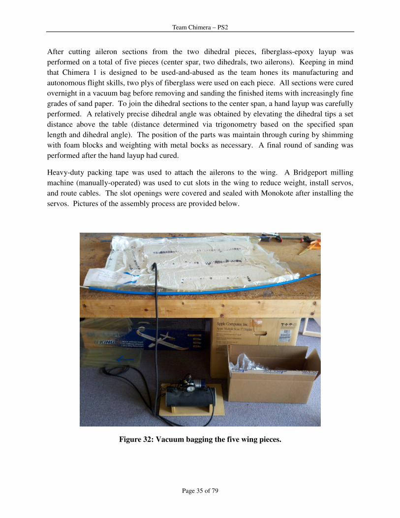
After cutting aileron sections from the two dihedral pieces, fiberglass-epoxy layup was
performed on a total of five pieces (center spar, two dihedrals, two ailerons). Keeping in mind
that Chimera 1 is designed to be used-and-abused as the team hones its manufacturing and
autonomous flight skills, two plys of fiberglass were used on each piece. All sections were cured
overnight in a vacuum bag before removing and sanding the finished items with increasingly fine
grades of sand paper. To join the dihedral sections to the center span, a hand layup was carefully
performed. A relatively precise dihedral angle was obtained by elevating the dihedral tips a set
distance above the table (distance determined via trigonometry based on the specified span
length and dihedral angle). The position of the parts was maintain through curing by shimming
with foam blocks and weighting with metal bocks as necessary. A final round of sanding was
performed after the hand layup had cured.
Heavy-duty packing tape was used to attach the ailerons to the wing. A Bridgeport milling
machine (manually-operated) was used to cut slots in the wing to reduce weight, install servos,
and route cables. The slot openings were covered and sealed with Monokote after installing the
servos. Pictures of the assembly process are provided below.
Figure 32: Vacuum bagging the five wing pieces.
Team Chimera – PS2
Page 36 of 79
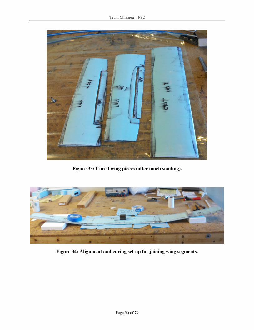
Figure 33: Cured wing pieces (after much sanding).
Figure 34: Alignment and curing set-up for joining wing segments.

Team Chimera – PS2
Page 37 of 79
Figure 35: Joined wing piece.
Figure 36: Milling slots for servo installation.

Team Chimera – PS2
Page 38 of 79
Figure 37: Fixturing for wing machining.
Fuselage. The fuselage external shape was cut from expanded polystyrene using the foam
cutter. The same milling machine that was used on the wing was then used to hollow out an
internal cavity to make room for avionics, servos, batteries, and propulsion hardware. Additional
modifications were made by hand using hobby knives and drill bits.
Figure 38: Cutting the external shape of the fuselage.
Team Chimera – PS2
Page 39 of 79
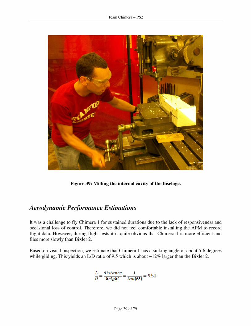
Figure 39: Milling the internal cavity of the fuselage.
Aerodynamic Performance Estimations
It was a challenge to fly Chimera 1 for sustained durations due to the lack of responsiveness and
occasional loss of control. Therefore, we did not feel comfortable installing the APM to record
flight data. However, during flight tests it is quite obvious that Chimera 1 is more efficient and
flies more slowly than Bixler 2.
Based on visual inspection, we estimate that Chimera 1 has a sinking angle of about 5-6 degrees
while gliding. This yields an L/D ratio of 9.5 which is about ~12% larger than the Bixler 2.

Team Chimera – PS2
Page 40 of 79
We are fortunate to have an experienced RC pilot on the team and he estimated Chimera 1’s stall
speed to be about 5.5 m/s.
For 15 °C, ρ = 1.225 kg/m3, S=0.266, W=0.748 kg *9.8=7.33 N, we estimate Chimera 1’s CL,max
to be about 1.48
Notes from RC Flight Testing & Considerations for Future Design
Iterations
The most noticeable observation from Chimera 1 flight tests was its lack of responsiveness and
the difficulty to make turns. This may be due to a combination of factors which include: (a) too
large of a dihedral that resists banking, (b) ailerons being too small, (c) pliant tail wings and
boom in the propeller wake, (d) wind gusts, and (e) trimming the neutral positions for the control
surface servos.
During the first few flights before setting the trims, Chimera 1 kept banking to the left and was
not responsive to RC commands to turn bank right. Out of curiosity, we shifted the rubber band-
mounted wing off center about 1 or 2 cm to the left so that more lift generated on the left wing
would oppose this tendency to bank left. This proved somewhat successful to cause Chimera 1 to
fly straight. Interestingly, at low speeds Chimera 1 would revert to its left banking tendencies but
at higher speeds the plane was more controllable, though it still lacked responsiveness. This is
due to the velocity dependence of lift.
After re-centering the wing and adjusting the trims, Chimera 1 was able to fly straight again
albeit still lacking responsiveness. It is worthwhile to mention that getting Chimera 1 to turn
involved moving the ailerons to maximum deflection. We did not try turning with the rudder
because on the Futaba controller, it is difficult to move the rudder without affecting the throttle.
Occasionally we would lose control of Chimera 1 for a few moments. We think this could be due
to separation due to maxing out the ailerons or gusts of wind.
To improve the responsiveness and turning radius of Chimera, we plan to implement a smaller
dihedral on the next wing design iteration. The dihedral will be reduced from 50cm dihedral
sections at a 10 degree angle to 30cm sections at a 6 degree angle. We plan to transition to balsa
wood construction for significant weight savings. As delineated in Task 2, we estimate a balsa
wing of the same design as Chimera 1 to be 120 grams. This would be less than half the weight
of our current 265 gram fiberglass-reinforced foam wing. During construction, we also plan to
add winglets for reduced drag.

Team Chimera – PS2
Page 41 of 79
The new balsa wing will include longer ailerons, extended from 2.5cm ailerons on a 18cm chord
to 3cm ailerons on a 16cm chord. This should improve responsiveness as well as prevent
separation around the wing, because the ailerons will not need to be actuated as extremely.
Meanwhile a quick fix for more flight testing with Chimera 1 would be to extend the ailerons
with tape and balsa wood.
Chimera 2 will feature a redesign of horizontal and vertical tails. We are still debating between
materials selection. A balsa tail would prove to be lighter weight, whereas a foam wing would
allow us to use a NACA 0008 symmetric airfoil for reduced drag. The vibrational and torsional
rigidity of the boom and tail wings will be addressed in our next prototype in the following two
ways. First, our boom will employ a square carbon fiber rod that has a larger moment of inertia.
Second, we will avoid expanded polystyrene foam because the square rod provides a flat
mounting surface. Alternatively will use extruded polystyrene, which is more dimensionally
stable, should we choose to include a mounting block.
Figure 40: Chimera 1 on its virgin flight!
Team Chimera – PS2
Page 42 of 79
Task 5: Closing Control Loops Primary contributors: Jack Tsai and Norman Wong
Before we derive a control law for altitude, heading and airspeed hold, we must obtain the
equations of motion for the aircraft. Having the equations, we can form the transfer function
between control surface displacement and attitude change.
Longitudinal Motion
The stick-fixed linearized longitudinal equation of motion can be represented in the state-space
form:
� Altitude Hold
We make the following assumption to derive a control law that maintains a desired altitude:
1. Altitude is a function of elevator input only, we decouple the input of the throttle
for the sake of simplicity.
2. Neglect the longitudinal-lateral coupling motion; that is, we restrict out aircraft
motion to the vertical plane.
For short period dynamics,
Taking the Laplace transform and dividing by yields our transfer function from elevator
input to pitch rate :
Team Chimera – PS2
Page 43 of 79
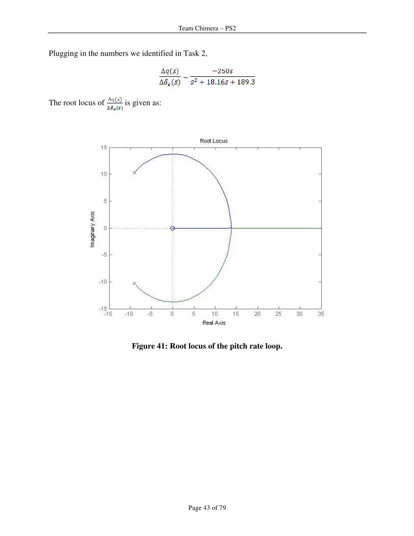
Plugging in the numbers we identified in Task 2,
The root locus of is given as:
Figure 41: Root locus of the pitch rate loop.

Team Chimera – PS2
Page 44 of 79
Since the DC gain is already negative, we apply a negative proportional gain to make the
closed loop stable for all gains. This modified root locus is shown below.
Figure 42: Negative root locus of the pitch rate loop.
Since ,
Our block diagram for the pitch feedback loops is shown as:
Team Chimera – PS2
Page 45 of 79
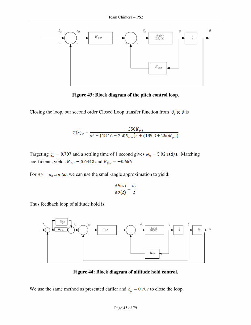
Figure 43: Block diagram of the pitch control loop.
Closing the loop, our second order Closed Loop transfer function from is
Targeting and a settling time of 1 second gives . Matching
coefficients yields and .
For , we can use the small-angle approximation to yield:
Thus feedback loop of altitude hold is:
Figure 44: Block diagram of altitude hold control.
We use the same method as presented earlier and to close the loop.
Team Chimera – PS2
Page 46 of 79
Simulation in SIMULINK:
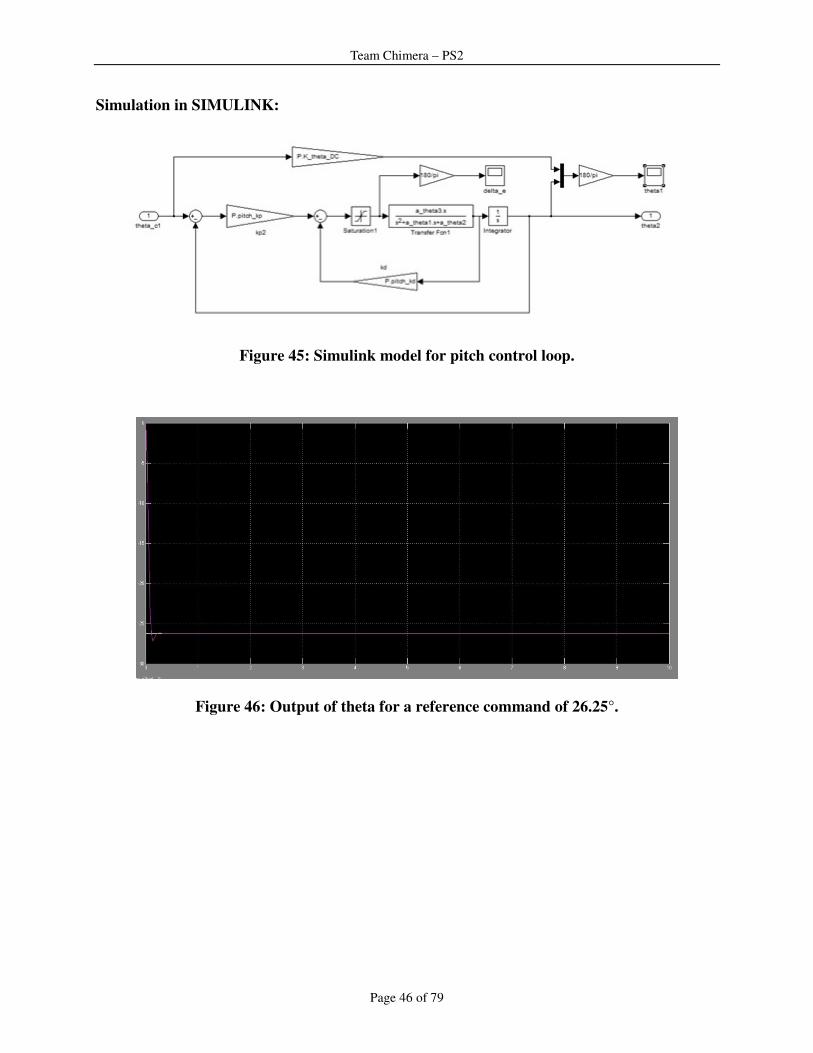
Figure 45: Simulink model for pitch control loop.
Figure 46: Output of theta for a reference command of 26.25°.
Team Chimera – PS2
Page 47 of 79
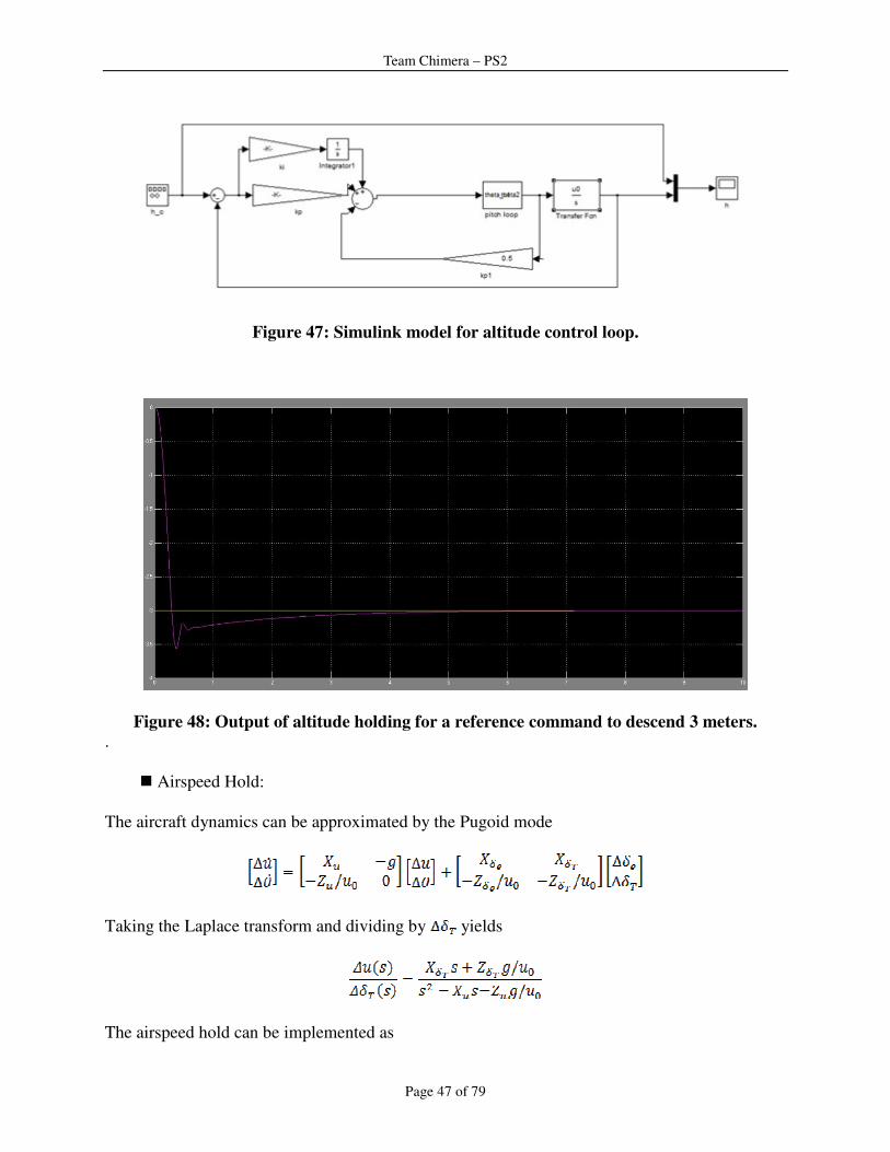
Figure 47: Simulink model for altitude control loop.
Figure 48: Output of altitude holding for a reference command to descend 3 meters.
.
� Airspeed Hold:
The aircraft dynamics can be approximated by the Pugoid mode
Taking the Laplace transform and dividing by yields
The airspeed hold can be implemented as
Team Chimera – PS2
Page 48 of 79
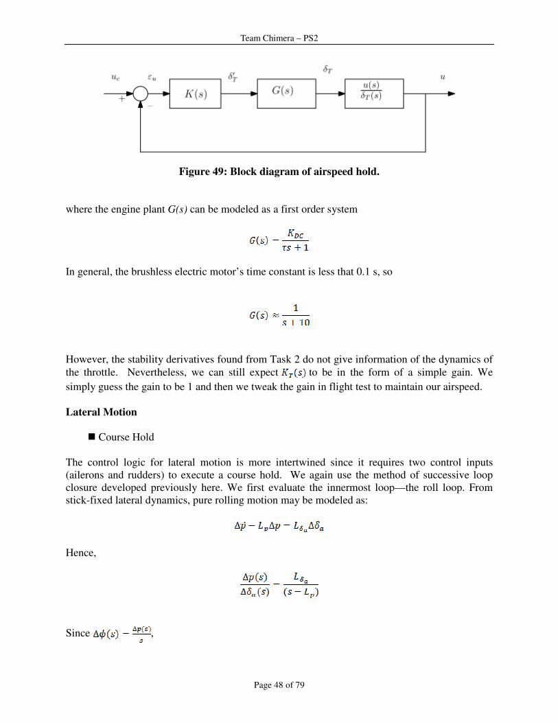
Figure 49: Block diagram of airspeed hold.
where the engine plant G(s) can be modeled as a first order system
In general, the brushless electric motor’s time constant is less that 0.1 s, so
However, the stability derivatives found from Task 2 do not give information of the dynamics of
the throttle. Nevertheless, we can still expect to be in the form of a simple gain. We
simply guess the gain to be 1 and then we tweak the gain in flight test to maintain our airspeed.
Lateral Motion
� Course Hold
The control logic for lateral motion is more intertwined since it requires two control inputs
(ailerons and rudders) to execute a course hold. We again use the method of successive loop
closure developed previously here. We first evaluate the innermost loop—the roll loop. From
stick-fixed lateral dynamics, pure rolling motion may be modeled as:
Hence,
Since ,
Team Chimera – PS2
Page 49 of 79
From Task 2, the dimensional stability and control derivatives are found and the transfer function
is :
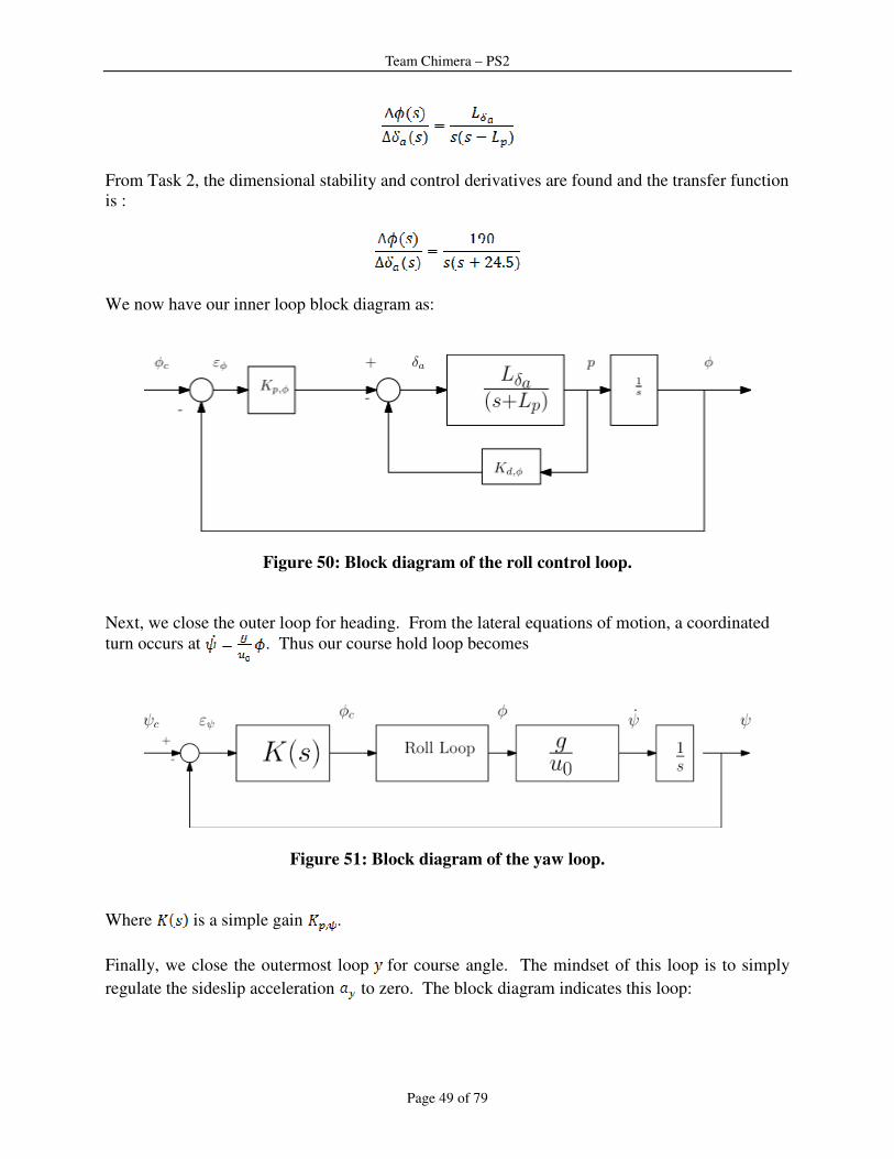
We now have our inner loop block diagram as:
Figure 50: Block diagram of the roll control loop.
Next, we close the outer loop for heading. From the lateral equations of motion, a coordinated
turn occurs at . Thus our course hold loop becomes
Figure 51: Block diagram of the yaw loop.
Where is a simple gain .
Finally, we close the outermost loop for course angle. The mindset of this loop is to simply
regulate the sideslip acceleration to zero. The block diagram indicates this loop:
Team Chimera – PS2
Page 50 of 79
Figure 52: Block diagram of the sideslip loop.
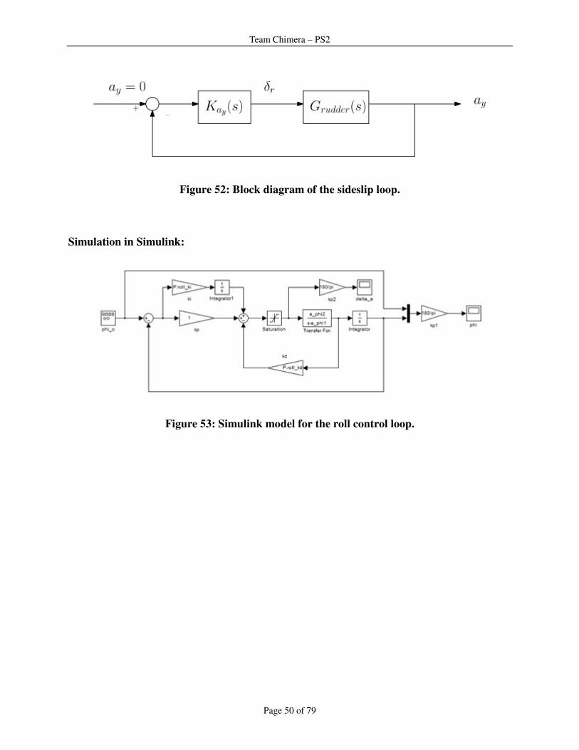
Simulation in Simulink:
Figure 53: Simulink model for the roll control loop.
Team Chimera – PS2
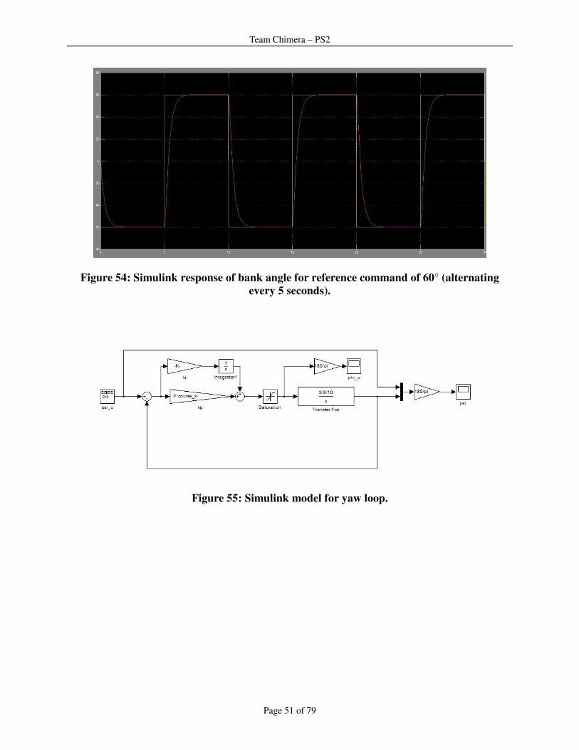
Page 51 of 79
Figure 54: Simulink response of bank angle for reference command of 60° (alternating
every 5 seconds).
Figure 55: Simulink model for yaw loop.
Team Chimera – PS2
Page 52 of 79
Figure 56: Simulink response of yaw angle for a refrence command of 30° (alternating
every 25 seconds).
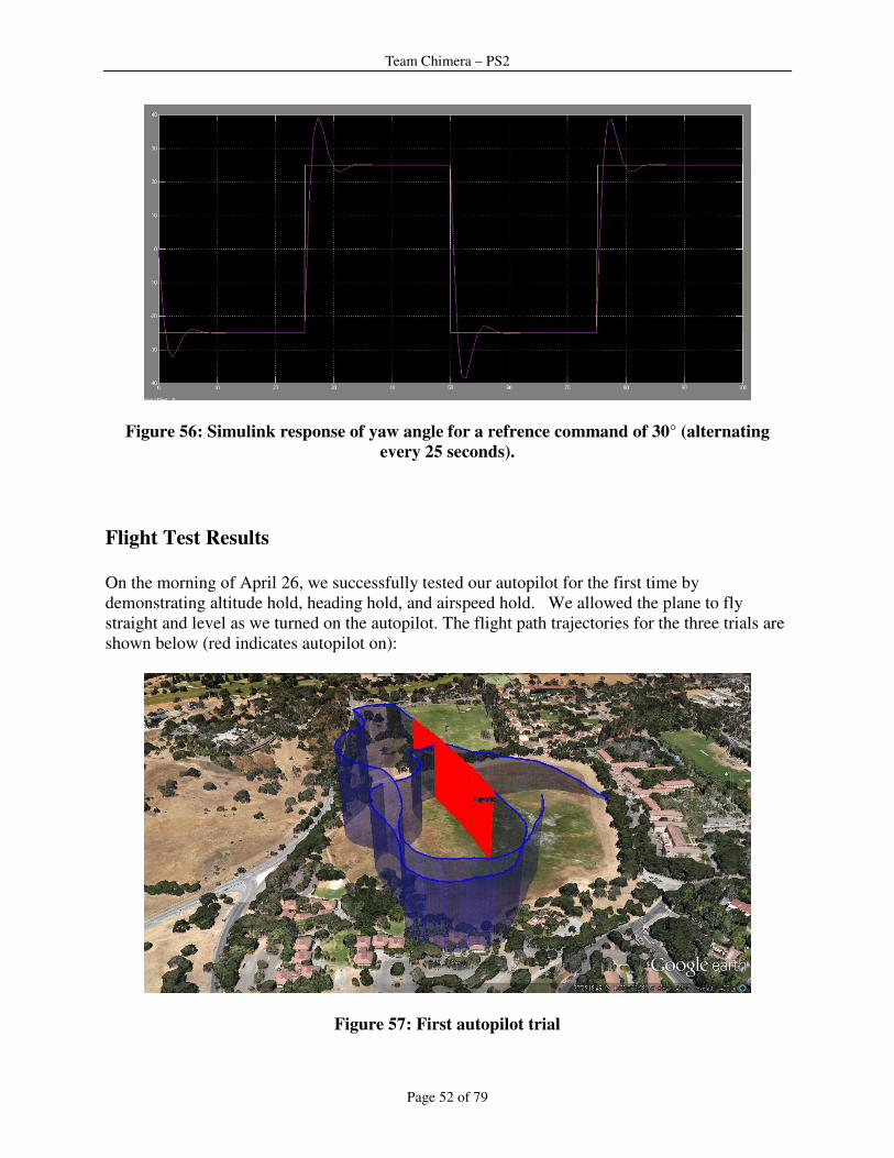
Flight Test Results
On the morning of April 26, we successfully tested our autopilot for the first time by
demonstrating altitude hold, heading hold, and airspeed hold. We allowed the plane to fly
straight and level as we turned on the autopilot. The flight path trajectories for the three trials are
shown below (red indicates autopilot on):
Figure 57: First autopilot trial
Team Chimera – PS2
Page 53 of 79
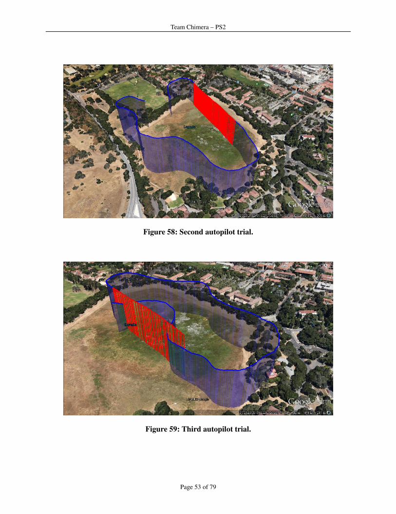
Figure 58: Second autopilot trial.
Figure 59: Third autopilot trial.
Team Chimera – PS2
Page 54 of 79
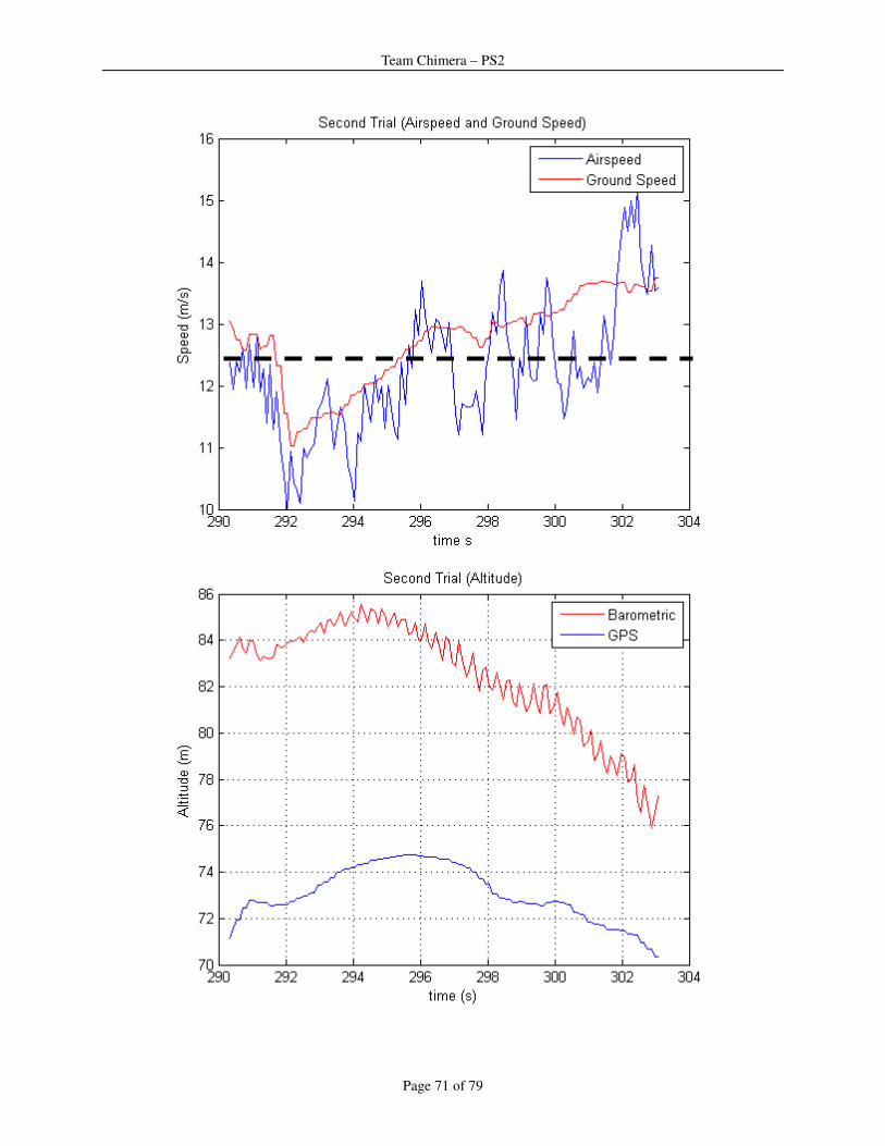
The altitude and airspeed for these flight trials is provided as Appendix A. Although the lateral
autopilot works perfectly, the longitudinal motion seems a slightly underdamped; the elevator
fluctuated severely which caused the tail to wobble far too much. After decreasing the gain of
the pitch loop, the wobbling of the tail was mitigated in the afternoon trial. Generally speaking,
the three trials for autonomous control were successful.
In the afternoon of April 26, the autopilot was tested for the second time to demonstrate the altitude hold,
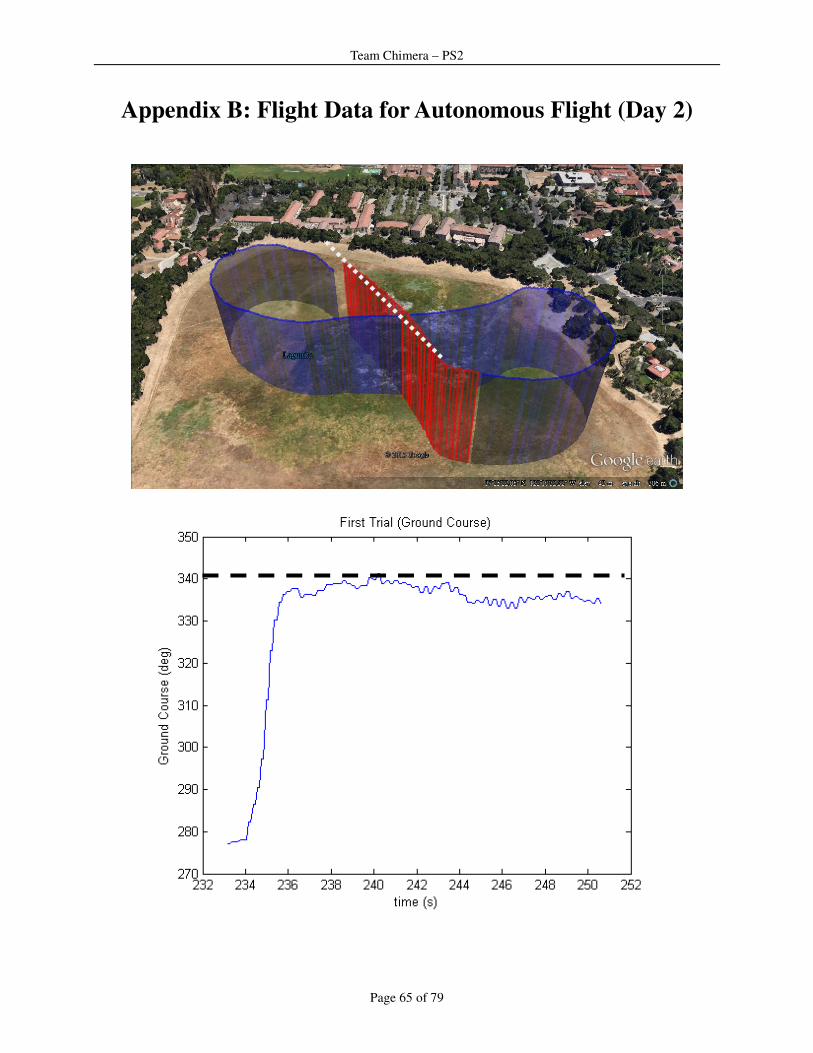
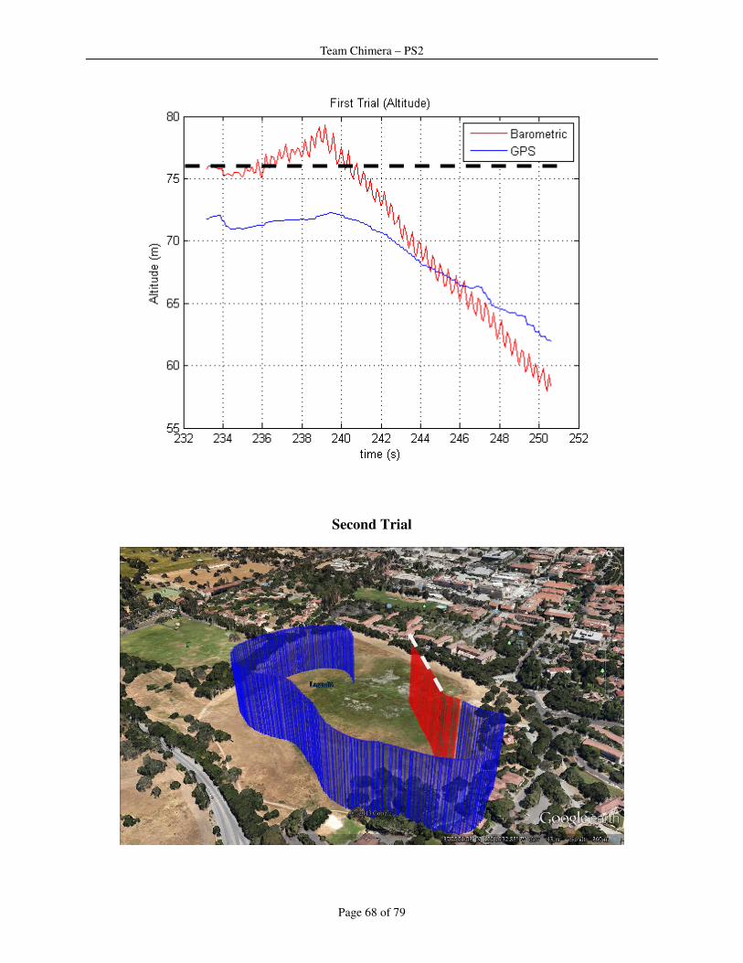
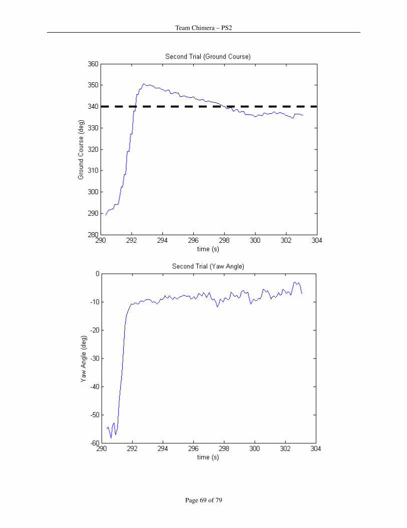
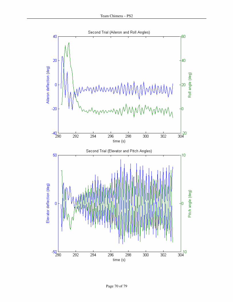
course hold (reference course angle 340°), and airspeed hold. The plane was allowed to fly straight and
level before turning on the autopilot. The flight path trajectory of the three trials along with plots of
control input/output data are provided as Appendix B.
As can be seen from the altitude plot, the altitude continues to decrease after turning. Therefore, the Kp,h
should be increased in future flight tests. Also, the fluctuations in the elevator are decreased in the last
trial, so there is still need to modify the gains in the pitch loop to smooth out the response. However, the
course angle was successfully held at 340°.
References:
[1] Robert C. Nelson, Flight stability and automatic control, McGraw-Hill Ryerson, Limited, 1989.
[2] Bernard Etkin, Lloyd Duff Reid, Dynamics of Flight: Stability and Control, Wiley, Oct 31, 1995.
Team Chimera – PS2
Page 55 of 79
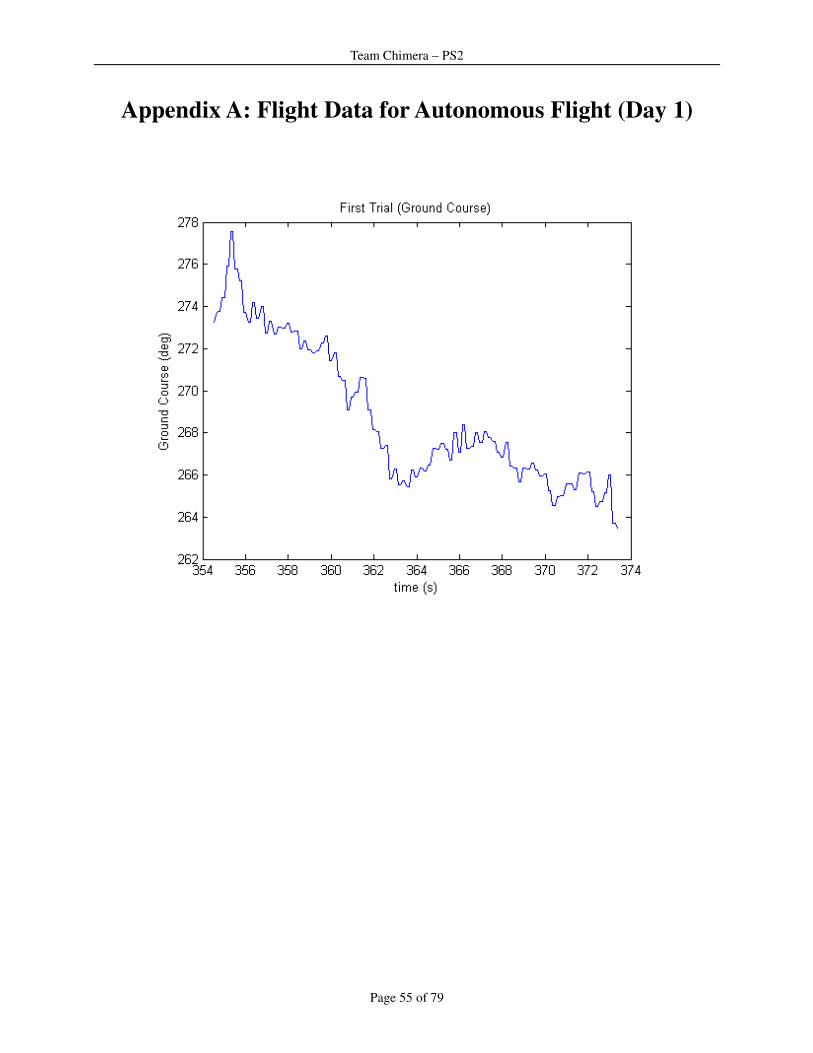
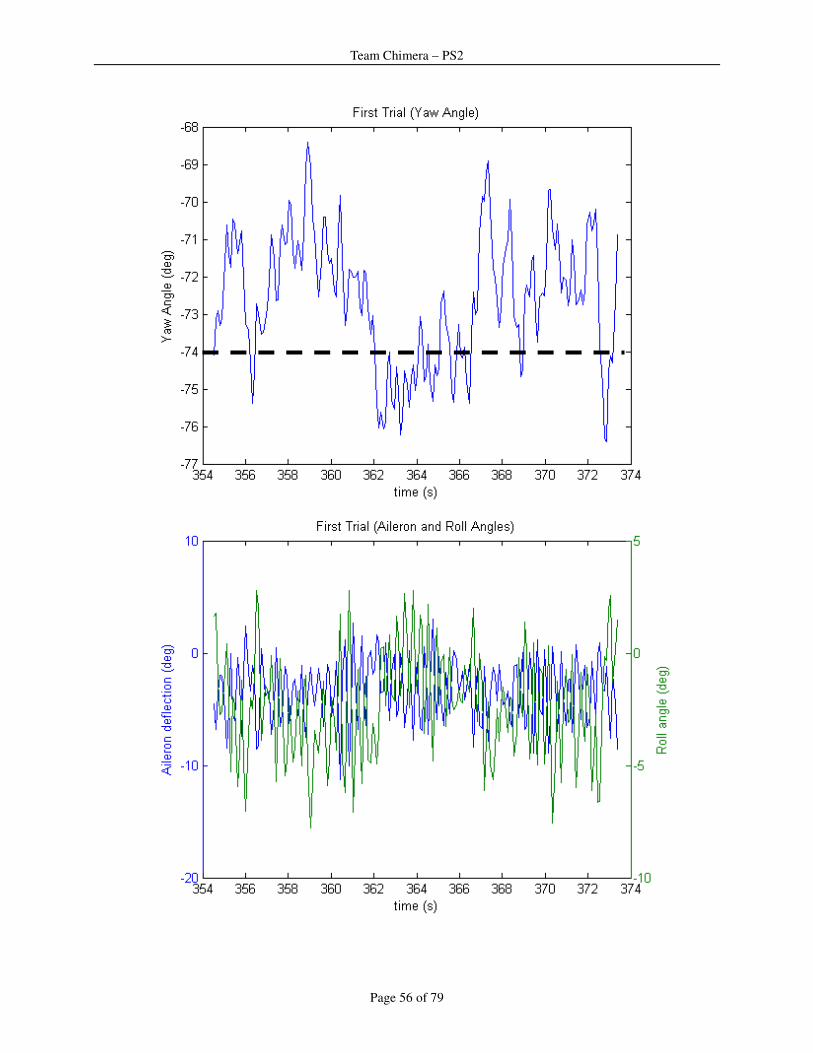
Appendix A: Flight Data for Autonomous Flight (Day 1)
Team Chimera – PS2
Page 56 of 79

Team Chimera – PS2
Page 57 of 79

Team Chimera – PS2
Page 58 of 79

Team Chimera – PS2
Page 59 of 79
Team Chimera – PS2
Page 60 of 79
Team Chimera – PS2
Page 61 of 79
Team Chimera – PS2
Page 62 of 79

Team Chimera – PS2
Page 63 of 79
Team Chimera – PS2
Page 64 of 79
Team Chimera – PS2
Page 65 of 79
Appendix B: Flight Data for Autonomous Flight (Day 2)

Team Chimera – PS2
Page 66 of 79

Team Chimera – PS2
Page 67 of 79
Team Chimera – PS2
Page 68 of 79
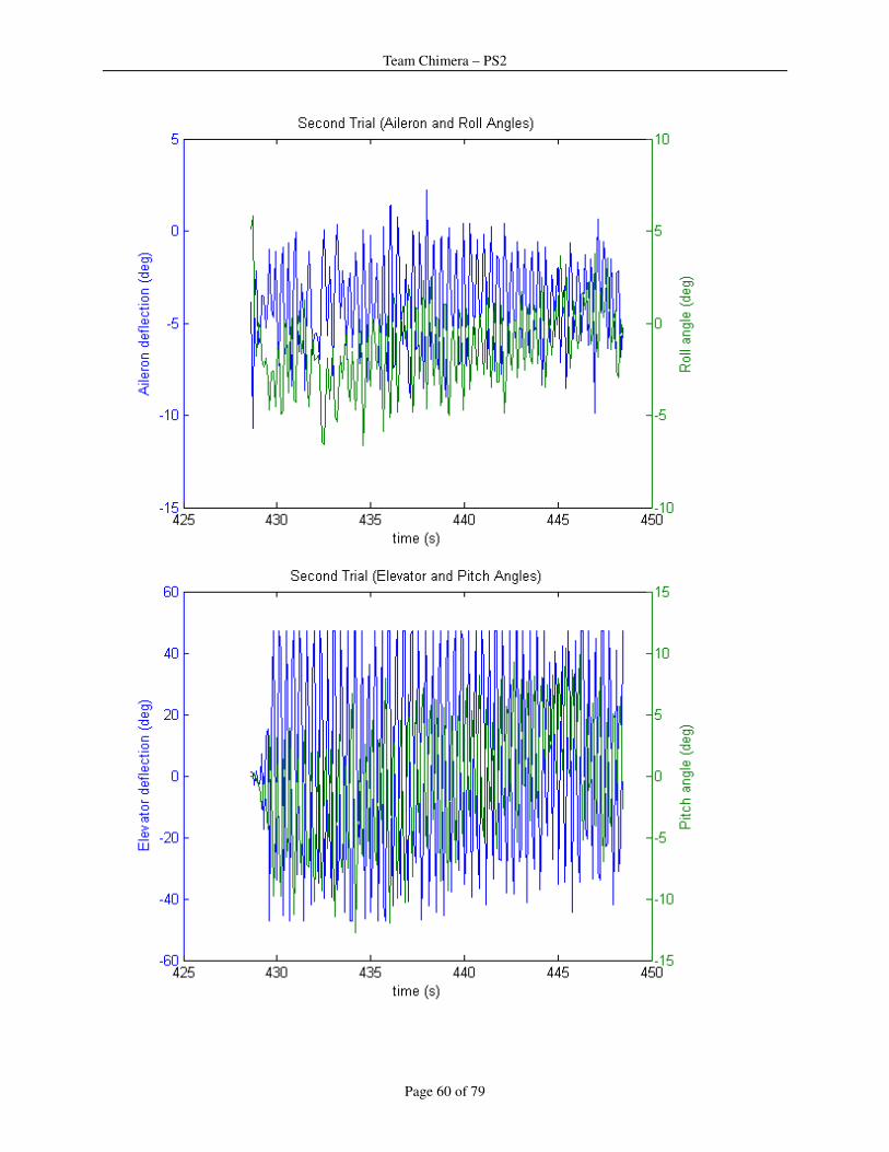
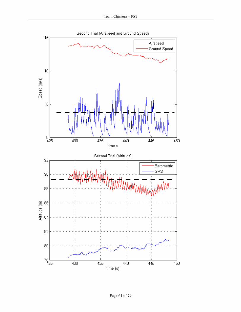
Second Trial
Team Chimera – PS2
Page 69 of 79
Team Chimera – PS2
Page 70 of 79
Team Chimera – PS2
Page 71 of 79
Team Chimera – PS2
Page 72 of 79
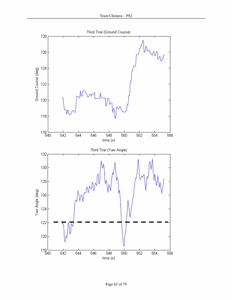
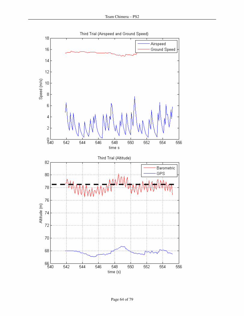
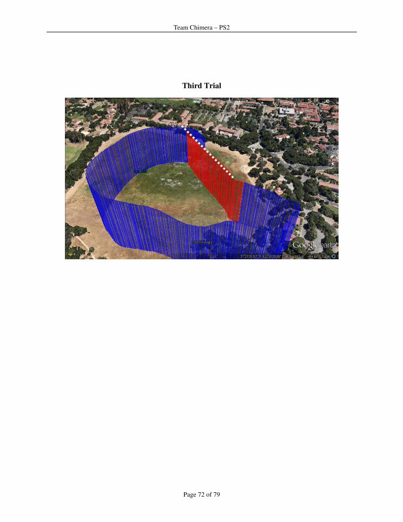
Third Trial

Team Chimera – PS2
Page 73 of 79
Team Chimera – PS2
Page 74 of 79
Team Chimera – PS2
Page 75 of 79
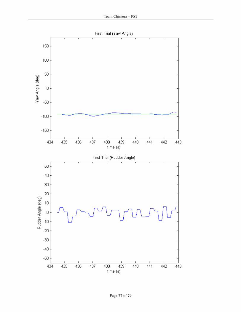
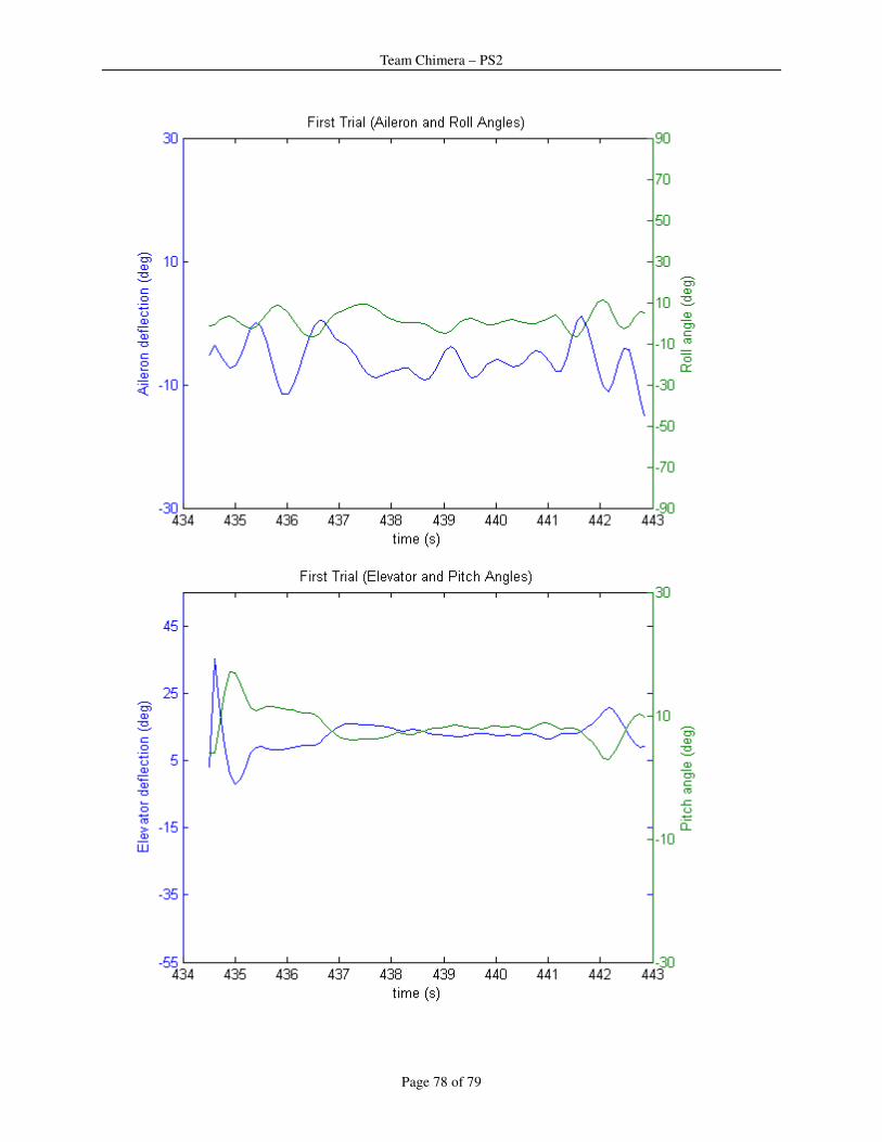
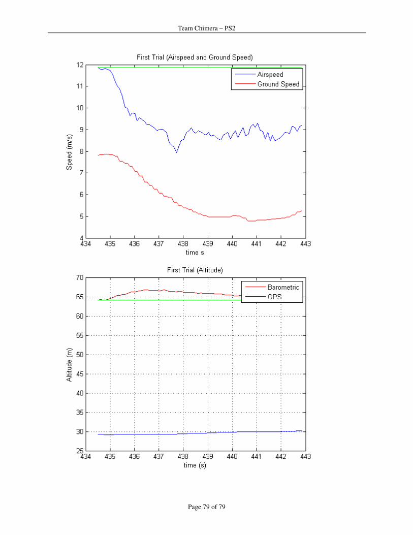
Team Chimera – PS2
Page 76 of 79
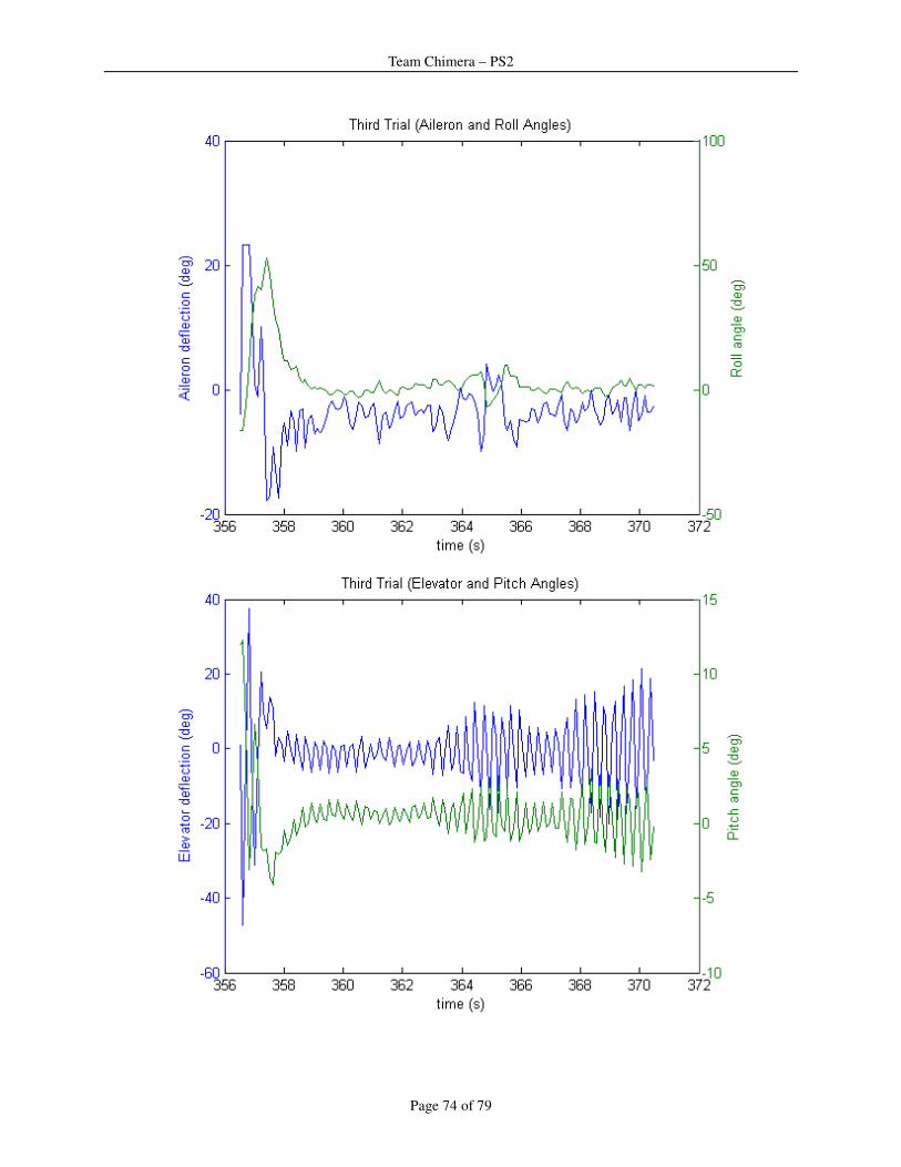
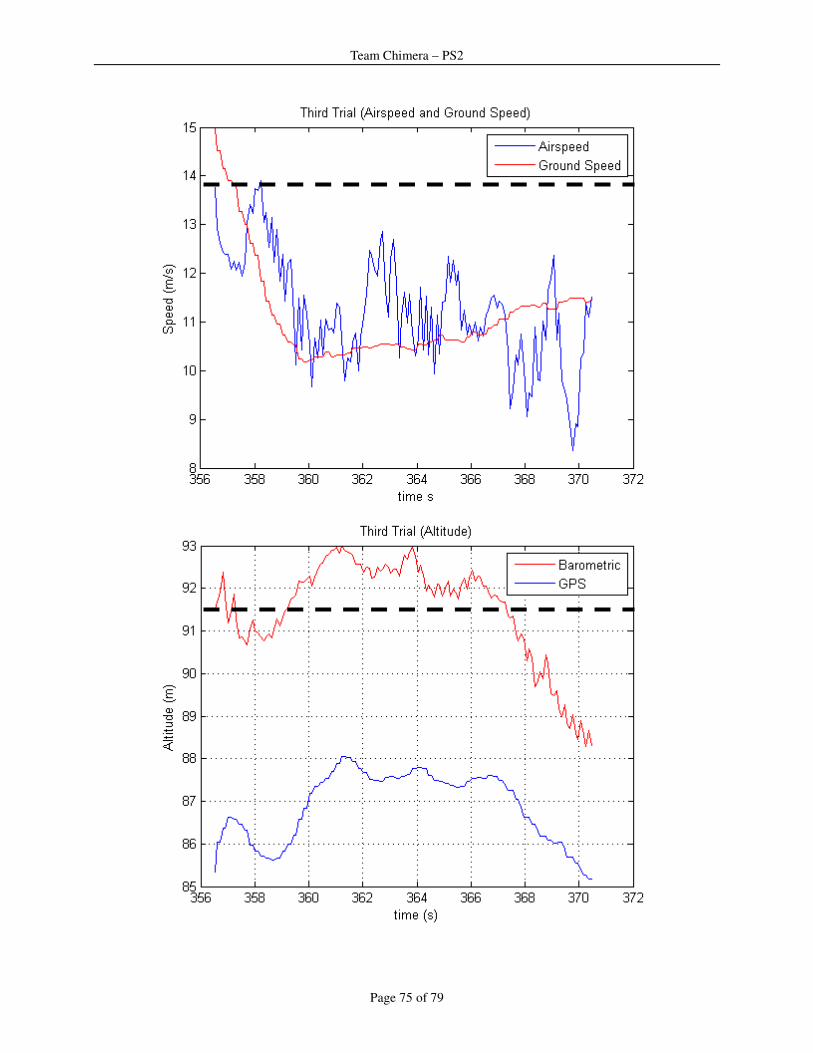
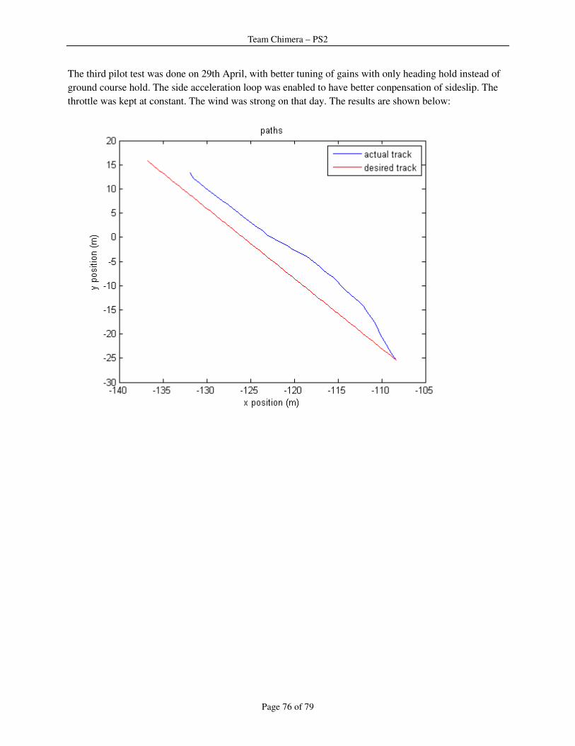
The third pilot test was done on 29th April, with better tuning of gains with only heading hold instead of
ground course hold. The side acceleration loop was enabled to have better conpensation of sideslip. The
throttle was kept at constant. The wind was strong on that day. The results are shown below:
Team Chimera – PS2
Page 77 of 79
Team Chimera – PS2
Page 78 of 79
Team Chimera – PS2
Page 79 of 79