a uniform geometrical theory of diffraction for an---1.pdf

$: A Uniform Geometrical Theory of Diffraction for an---1.pdf$
1448 PROCEEDINGS OF THE IEEE, VOL. 62, NO. 11, NOVEMBER 1974

A Unifm Geometrical Theory of Diffraction for an Edge in a Perfectly Conducting Surface

Abrmct-A compact dyadic diffraction coefficient for electromagnetic wnea oblique& incident on a cauved fmned by perfectly conducting c w e d or plane dace4 is obtained. This diffraction coefficient rem& VW in the trrnsition regions adjacent to shadow and reflection boundnies, where the diffhction d s c i e n t s of Kella’s originrl theory fail. Our method is based on Keller’s method of the anonid problem, which in this case is the perfectly conducting wedge illuminated by plpne, cylindrical, conical, md sphedcrl waves When the p m p r ray-ked coordinate system is introduced, the dyrdic diffraction d i c i e n t for the wedge is found to betheaunofoalytwody.ds,anditislown(hrtthisisrlsotmefor the dyadic diffraction coefficients of higher order edges One dyad contains the acoustic soft diffraction coef f int ; the other dyad contains the acoustic hard diffraction coefficient The expressions for the amustic wedge diffraction coefficients contain Fremelintegrds,which ensure that the total field is continuous at shadow and reflection bou- The diffraction coeffiiients have the same form for the different types of edge illumination; only the arguments of the Fresnel integrals are different Since diffraction is a l d phenomenon, and locally the curved edge structure is wedge shaped, this result is readily extended to the curved wedge. It is interesting that wen though the polntivtions pnd the wavefront curvatures of the incident, reflected, and diffracted waves are markedly different, the total field calculated from this high-frequency solution for the curved wedge is continuous at shadow and reflection boundaries.

I. INTRODUCTION HIS PAPER is concerned with the construction of a high-frequency solution for the diffraction of an electromagnetic wave obliquely incident on an edge in an

otherwise smooth curved perfectly conducting surface sur- rounded by an isotropic homogeneous medium. The surface normal is discontinuous at the edge, and the two surfaces forming the edge may be convex, concave, or plane. The solution is developed within the context of Keller’s geometrical theory of diffraction (GTD) [ 11 -[3] so the dyadic diffraction coefficient is of interest. Particular emphasis is placed on finding a compact accurate form of the diffraction coefficient valid in the transition regions adjacent to shadow and reflection boundaries and useful in practical applications. In treating this problem the wedge was considered f i t ; its solution was extended later to the curved wedge.’

According to the GTD, a high-frequency electromagnetic wave incident on an edge in a curved surface gives rise to a reflected wave, an edge diffracted wave, and an edge excited wave which‘ propagates along a surface ray. Such surface ray

initial work on the solutions of the canonical problems was sup Manuscript received July 3, 1974; revised August 1, 1974. The

ported in part by Contract AF 19(628)-5929 between Air Force

search Foundation; the subsequent work on the generalization of these Cambridge Research Laboratories and The Ohio State University Re-

solutio^ was supported in part by Grant NGR 36-008-144 between NASA and The Ohio State Univmity Research Foundation.

The authors are with the ElectroScience Laboratory and the De- partment of Electrical Engineering, Ohio State University, Columbus, Ohio 43212.

the edge is curved. ‘ The t a m ‘‘curved wedge” is used when one of the surfaces forming

sr

EDGE E< ft” (SURFACE NORMAL

Sd DISCONTINUOUS)

Fig. 1. Incident, reflected, and diffkacted rays and their associaqd shadow and reflection boundaries projected onto the plane normal to the edge at the point of diffraction QE.

fields may also be excited at shadow boundaries of the curved surface. The problem is easily visualized with the aid of Fig. 1, which shows a plane perpendicular to the edge at the point of diffraction QE. The pertinent rays and boundaries are projected onto this plane. To simplify the discussion of the reflected field, we have assumed that the local interior wedge angle is < A. According to Keller’s generalized Fermat’s principle, the ray incident on the edge QE produces edge diffracted rays ed and surface diffracted rays sr. In the case of convex surfaces, the surface ray sheds a surface diffracted ray sd from each point Q on its path. ES is the boundary between the edge diffracted rays and the surface diffracted rays; it is tangent to the surface at QE. SB is the shadow boundary of the incident field and RB is the shadow boundary of the reflected field, referred to, henceforth, simply as the reflection boundary. If both surfaces are illuminated, then there is no shadow boundary at the edge; instead there are two reflection boundaries for the problem considered here. Since the behavior of the ray optics field is different in the two regions separated by a boundary, there is a transition region adjacent to each boundary within which there is a rapid variation of the field between the two regions. In the present analysis it is assumed that the sources and

field point are sufficiently removed from the surface and the boundary ES so that the contributions from the surface ray field can be neglected. The total electric field may then be represented as

E = E i u i + E ’ u ’ + E d . (1)

In which E‘ is the electric field of the source in the absence of the surface, E‘ is the electric field reflected from the surface with the edge ignored,. and Ed is the edge diffracted electric field. The functions u’ and U‘ are unit step functions. which are equal to one in the regions illuminated by the incident and reflected fields and to zero in their shadow regions. The extent of these regions is determined by geometrical optics. The step functions are shown explicitly in (1) to em- phasize the discontinuity in the incident and reflected fields at

KOUYOUMJIAN AND PATHAK: GEOMETRICAL THEORY OF EDGE DIFFRACTION 1449

the shadow and reflection boundaries, respectively. They are not included in subsequent equations for reasons of notational economy.

The diffracted field as defined by (1) penetrates the shadow region, which according to geometrical optics, has a zero field to account for the nonvanishing fields known to exist there. But the correct high-frequency field must be continuous at the shadow and reflection boundaries; hence the diffracted field must also compensate for the discontinuities in the incident and reflected fields there. In other words, the diffracted field must provide the correct transition between the illuminated regions and the regions shadowed by the edge.

The high-frequency solution described in the next sections is obtained in the following way. A Luneberg-Kline expansion [41 for the incident field is assumed to be given. The reflected field is expanded similarly and related to the incident field by imposing the boundary condition at the perfectly conducting surface. Only the leading term is retained. Next the general form of the leading term in the high-frequency solution for the edge diffracted electromagnetic field is determined. The wedge (formed by the intersection of two plane surfaces) is treated first; its dyadic diffraction coefficient is deduced from the asymptotic solution of several canonical problems. Some parameters in this diffraction coefficient are seen to depend on the type of edge illumination. They are determined for an arbitrary incident wavefront by requiring the leading term in the total field to be continuous at the shadow and reflection boundary. It is found that only a slight extension of the solution for the wedge is needed to treat the more general problem posed by the curved edge. This paper follows in a natural way from some earlier work.

In [SI the Pauli-Clemmow method of steepest descent was employed in a manner different from that employed by Pauli [61 to obtain a more accurate asymptotic solution for the field diffracted by a wedge. We showed that our generalized Pauli expansion can be transformed term by term into a generalized form of the asymptotic expansion given by Ober- hettinger [71. The leading term in our expansion was found to be more accurate than the leading term in Oberhettinger's expansion; furthermore, our leading term for the diffracted field contains a simple correction factor, which permits the field to be calculated easily in the transition region. This property is of considerable practical importance, because it enables one to use the GTD in the transition regions without introducing a supplementary solution. The correction factors, referred to here as transition functions, are simply included with the diffraction coefficient.

In [SI only the scalar problem of plane waves normally incident of the edge of the wedge is considered. In [ 8 ] , this work is extended to obtain a dyadic diffraction coefficient for a perfectly conducting wedge illuminated by obliquely incident plane, conical, and spherical waves. By introducing the natural ray-fixed coordinates, the dyadic diffraction coefficient obtained from each of these canonical problems is reduced to the sum of two dyads. In other words, the matrix formed by the elements of the dyadic diffraction coefficient is a two by two diagonal matrix. The diagonal elements of this matrix are simply the scalar diffraction coefficients Dh and D, for the Neumann (hard) and Dirichlet (soft) boundary conditions, respectively. The transition functions appearing in D, and D h have the same form for the four types of illumination; in each case only a Fresnel integral is involved. However, the argument of the Fresnel integral depends upon the type of illu-

mination. Outside of the transition regions these factors are approximately one, and Keller's expressions for the diffraction coefficients are obtained. The asymptotic solutions described in this paragraph help us formulate the solution for a more general type of illumination of the wedge, as noted earlier.

The analysis of wedge diffraction has had a lengthy history. Only a few of the reports and papers have been mentioned thus far. Many of the more important papers on this subject may be found in [ 91 and [ 101 . A good review of wedge diffraction and the special case of half-plane diffraction is given in [9, chs. 6 and 81. Recently, Ahluwalia, Boersma, and Lewis have written some papers [11]-[ 131 of special rele- vance to the work described here. In [ 111 and [ 121 high- frequency asymptotic expansions for scalar waves diffracted by curved edges in plane and curved screens are described, and this work is extended to a curved edge in a curved surface in [ 131. The authors make use of ray coordinates, and some of their results dealing with rays and wavefronts have been help- ful in the development of our solution. Nevertheless, there are some noteworthy differences between their solutions and ours, apart from the fact that their problem is scalar instead of the vectorial problem treated here. Their formulation or ansatz begins with the total field, and the resulting correction of the ordinary GTD solution in the transition region is different from ours. Our result is related more directly to the form of the GTD solution; furthermore, it appears to be more accurate when only the leading term in the two asymptotic expansions is retained.

11. THE GEOMETRICAL-~PTICS FIELD The geometrical-optics field, which is the sum of the leading

terms in the asymptotic expansions for the incident and reflected fields, is a part of our high-frequency solution for edge diffraction. The incident and reflected electric fields are expanded in Luneberg-Kline series

where an exp (jut) time dependence is assumed and k is the wavenumber of the medium. Substituting the preceding expansion into the vector wave equation for the electric field and integrating the resulting transport equation for m = 0 [ 141, [ 151, the leading term in (2) is

E(s) - ~ X P [-jkJl(s)l Eo(s) = Eo (0)

which is recognized as the geometrical-optics field. Here s is the distance along the ray path and pl , p z are the principal radii of curvature of the wavefront at the reference point s = 0. In Fig. 2, p1 and p z are shown in relationship to the rays and wavefronts

It is apparent that when s = -pl or - p z , (3) becomes infinite so' that it is no longer a valid approximation. The intersection of the rays at the lines 1-2 and 3-4 of the astigmatic tube of rays is called a caustic. As we pass through a caustic in the direction of propagation the sign of p + s changes and the correct phase shift of +n/2 is introduced naturally. Equation (3) is a valid high-frequency approximation on either side of the caustic; the field at a caustic must be found from separate considerations [ 161 , [ 171 .

1450 PROCEEDINGS OF THE IEEE, NOVEMBER 1974

Fig. 2. Astigmatic t u b of nyr.

Fw. 3. Reflection at (I curved surface.

Employing the Maxwell curl equation V X E = -jam, it follows from (2) that the leading term in the asymptotic approximation for the magnetic field is

H-Yc?XE (4)

where Yc = is the characteristic admittance of the medium, ? is a unit vector in the direction of the ray path, and E is given by (3). From V * E = 0 one obtains

A s ' E o = o . ( 5 )

Let a high-frequency electromagnetic wave be incident on a smooth curved perfectly conducting surface S, which is part of our curved edge structure. The geometricalaptics electric field reflected at QR on S (see Fig. 3) has the form given by (3). Choosing QR to be the reference point, it follows from the boundary condition for the total electric field on S that

G ( o ) exp [ - ~ W ( O ) I = E'(QR) * E = E'(QR) * [ ell ell el ell

(6) in which Ei(QR) is the electric field incident at QR and Eis the dyadic reflection coefficient with gl the unit vector perpendicular to the plane of incidence and $/, g i the unit vectors parallel to the plane of incidence as shown in Fig. 3. In matrix notation

Ai A? - A A

From (3) and (6),

in which p i and p i are the principal radii of curvature of the reflected wavefront at the point of reflection Q R . The dependence of p i and p i on the incident wavefront curvature, the aspect of incidence and the curvature of S at QR is given in Appendix I.

In principle, the geometricalaptics approximations can be improved by finding the higher order termsE:(R), E;(R), - * , in the reflected field, but in general it is not easy to obtain

these from the higher order transport equations. Further- more, these terms do not correct the serious errors in the geometrical-optics field resulting from the discontinuities at reflection and shadow boundaries.

111. THE EDGE DIFFRACTED FIELD The smooth surface S has a curved edge formed by a discon-

tinuity in its unit normal vector. Equation (3) can be obtained in a quite different way which shows that it is also the leading term in the asymptotic approximation of the diffracted field. Using the method of stationary phase to evaluate the integral representation of the edge diffracted field over its wavefront one obtains

It is convenient to locate the reference point 0' at the edge point QE from which the diffracted ray emanates, see Fig. 4; however, the edge is a caustic of the diffracted field. On the other hand, it is clear that Ed($) given by (9) must be independent of the location of 0', hence, l h ~ , , l - , ~ Ed(O') f l ex- ists. Since the diffracted field is proportional to the field incident at Q E ,

lim ~ ~ ( 0 ' ) @ = E'(QE) - ii (10) p'+ 0

where 5 is the dyadic edge diffraction coefficient, which is analogous to the dyadic reflection coefficient of the preceding section. It is assumed here that E' is not rapidly varying at QE, except possibly for its phase variation along the incident ray.

Thus the edge diffracted electric field r

in which p is the distance between the caustic at the edge and the second caustic of the diffracted ray.

In 125, appendix 111, it is shown that

wherein p', is the radius of curvature of the incident wavefront at QE taken in the plane containing the incident ray and i: the unit vector tangent to the edge at QE, i& is the associated unit normal vector to the edge directed away from the center of curvature, 4 > 0 is the radius of curvature of the edge at QE, and 00 is the angle between the incident ray and the tangent to the edge as shown in Fig. 5(a). The unit vectors ?' and s ̂ are in the directions of incidence and diffraction, respectively. Equation (12) is seen to have the form of the elementary mirror and lens formulas in which fis the focal distance. if p is positive, there is no caustic along the diffracted ray path; however the caustic distance p is negative if the (second) caustic lies between QE and the observation point. The diffracted field calculated from (1 1) is not valid at a caustic, but as one moves outward from QE along the diffracted ray, a phase shift of + r / 2 is introduced naturally after the caustic is passed as in the case of the geometrid-optia field.

Since the high-frequency diffracted field has a caustic at the edge, (1 1) is not vali&there, and we cannot impose a condition at QE to determine D in a manner similar to that used to find


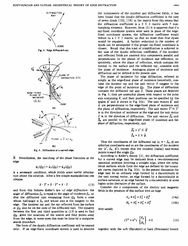
Fig. 4. Edge diffracted ray.

e

EDGE- FIXED

'ION

EDGE

(a)

n n

(b) Fig. 5. Diftkaction at a curved edge.

E. Nevertheless, the matching of the phase functions at the edge

$ i ( Q E ) = $ A Q E ) = $ ~ ( Q E )

is a necessary condition, which yields some useful informa- tion about the solution. After a few simple manipulations one obtains

3 . 3 ' = f . P ' = ^ e * s (1 3)

and from this follows Keller's law of edge diffraction: the angle of diffraction Pd is equal to the angle of incidence P O , so that the diffracted rays emanating from QE form a cone whose half-angle is Po and whose axis is the tangent to the edge. The incident ray and the ray reflected from the surface at QE also lie on the cone of the diffracted rays. The equality between the first and third quantities in (1 3) is used to fiid QE, given the locations of the source and field points away from the edge; in some cases this must be done by a computer search procedure.

The form of the dyadic diffraction coefficient will be treated next. If an edge-fixed coordinate system is used to describe

the components of the incident and diffracted fields, it has been found that the dyadic diffraction coefficient is the sum of seven dyads [ 181, [ 19 ] in the matrix form this means that the diffraction coefficient is a 3 X 3 matrix with 7 nonvanishing elements. However, from (5) it is apparent that if a ray-fixed coordinate system were used in place of the edge- fixed coordinate system, the diffraction coefficient would reduce to a 2 X 2 matrix, so that no more than four dyads would be required. A further reduction in the number of dyads can be anticipated if the proper ray-fixed coordinate is chosen. Recall that this kind of simplification is achieved in the case of the dyadic reflection coefficient, if the incident and reflected fields are resolved into components parallel and perpendicular to the planes of incidence and reflection, respectively, where the plane of reflection, which contains the normal to the surface and the reflected ray, coincides with the plane of incidence. Analogous planes of incidence and diffraction can be defined in the present case.

The plane of incidence for edge diffraction, referred to simply as the edge-fixed plane of incidence henceforth, contains the incident ray and the unit vector i: tangent to the edge of the point of incidence Q E . The plane of diffraction contains the diffracted ray and 3. These planes are depicted in Fig. 5 ; they are azimuthal planes with respect to the polar axis containing f , and their positions can be specified by the a$es 9' and $ shown in Fig. 5(b). The unit vectors 6' and 9 are perpendicular to the edge-fixed plane of incidence and the plane of diffraction, respectively. The unit vector 0' ?' is in the direction of incidence at the edge and the unit vector

is in the direction of diffraction. The unit vectors 8; and Po are parallel to the edge-fixed plane of incidence and the plane of diffraction, respectively, and

Thus the coordinates of the diffracted ray (s, A - P o , 9) are spherical coordinates and so are the coordinates of the incident ray (s', P o , $'), except that the incident (radial) unit vector points toward the origin QE .

According to Keller's theory [ 31, the diffraction coefficient for a curved edge may be deduced from a two-dimensional canonical problem involving a straight edge, where the cylindrical surfaces which form the edge are defined by the boundary curves depicted in Fig. 5(b). In the present discussion the edge may be an ordinary edge formed by a discontinuity in the unit normal vector, an edge formed by a discontinuity in surface curvature, or an edge formed by a discontinuity in some higher order derivative of the surface.

Consider the z components of the electric and magnetic fields in the presence of this surface with an edge

they satisfy

together with the soft (Dirichlet) or hard (Neumann) bound-

PROCEEDINGS OF THE IEEE, NOVEMBER 1974 1452

ary conditions

E, = 0 (16)

or

- = o an

respectively, on the boundary curve and the radiation condition at infinity. The a/an is the derivative along the normal to the boundary curve.

Starting with the high-frequency solutions for the z components of the diffracted field, substituting these into. (151, and employing the methods described earlier, the asymptotic solutions may be put into the form

in which D, is referred to as the soft scalar diffraction coefficient obtained when the soft boundary condition is used, and Dh is referred to as the hard scalar diffraction coefficient obtained when the hard boundary condition is used.

Since Ef = E;; sin 00 ( 1 W

and similarly for the z components of the diffracted field, it follows from (1 8) and (1 9) that

consequently, the dyadic diffraction coefficient for an ordinary (or higher order) edge in a perfectly conducting surface can be expressed simply as the sum of two dyads -

D = - $OD, - $ I $ & (21)

to fmt order. Since D, and Dh are the ordinary scalar diffraction coefficients which occur in the diffraction of acoustic waves which encounter soft or hard boundaries, we see the close connection between electromagnetics and acoustics at high frequencies. Also, it follows that the high-frequency diffraction by more general edge structures, and by thin curved wires can be described in the form given by (1 1) and (2 1).

The balance of this paper is concerned with finding expressions for D, and Dh which can be used in the transition regions adjacent to shadow and reflection boundaries in the case of diffraction by an ordinaIy edge. Recently, Keller and Kaminetzky [20] and Senior [21 I have obtained expressions for the scalar diffraction coefficients in the case of diffraction by an edge formed by a discontinuity in surface curvature, and Senior [22] has given the dyadic (or matrix) diffraction coefficient in an edge-fixed coordinate system. Keller and Kaminetzkey [201 also have given expressions for the scalar diffraction coefficients in the case of higher order edges.

The diffraction by a wedge will be considered first; the straight edge serves as a good introduction to the more difficult subject of diffraction by a curved edge. As noted earlier, the dyadic diffraction coefficient can be found from the asymptotic solution of several canonical problems, which involve the illumination of the edge by different wavefronts. It is not

difficult to generalize the resulting expressions for the scalar diffraction coefficients to the case of illumination by an arbitrary wavefront.

IV. THE WEDGE When a plane, cylindrical, or conical electromagnetic wave is

incident on a perfectly conducting wedge, the solution may be formulated in terms of the components of the electric and magnetic field parallel to the edge; we will take these to be the z components. In the case of a spherical wave it is convenient to use the z components of the electric and magnetic vector potentials. These z components may be represented by eigenfunction series obtained by the method of Green's functions. The Bessel and Hankel functions in the eigenfunction series are replaced by their integral representations and the series are then summed leaving the integral representations. Integral representations for the other field components in the edge-fixed coordinate system are then found from the z (or edge) components, except in the case of the incident spherical wave, where the integral representations of the field components are obtained from the z components of the vector potentials. These integrals are approximated asymptotically by the Pauli-Clemmow method of steepest descent [231, and the leading terms are retained. The field components are then transformed to the ray-fixed coordinate system described pre- viously. The resulting expression for the diffracted field can be written in the form of (1 1) which r@es it possible to deduce the dyadic diffraction coefficient D . The asymptotic solutions outlined in this paragraph are presented in detail [81.

- E'(Q=) E(?, f') A($) exp (-jks) (22)

in which A(s ) describes how the amplitude of the field varies along the diffracted ray;

1

Summarizing the results given in [ 8 I

for plane, cylindrical, and conical wave

incidence, s is replaced by r = s sin 00, the perpendicular distance to the edge) (23)

6' incidence (in the case of cylindrical wave

A($) =

d- , for spherical wave incidence.

It follows from (12) that p = p i for the. wedge. In the case of plane, cylindrical, and conical waves p: is infinite and in the case of2pherical waves pf = s'. The dyadic diffraction coefficient D(p, ? I ) has the form given in (21), which supports the assumptions leading to that equation.

If the field point is not close to a shadow or reflection boundary, the scalar diffraction coefficients [ 31

for all four types of illumination, which is important, because the diffraction coefficient should be independent of the edge illumination away from shadow and reflection boundaries where the plane surfaces forming the wedge are 4 = 0 and 4 = nn. The wedge angle is (2 - n) n; see Fig. 5(b). This ex-


pression becomes singular as shadow or reflection boundaries are approached, which further aggravates the difficulties at these boundaries resulting from the discontinuities in the incident or reflected fields. Combining (1 l ) , (2 l) , and (24), it is seen that outside the transition regions the diffracted field is of order k-lIz with respect to the incident and reflected fields. In (24) and in equations to follow the upper sign applies to

Grazing incidence, where 9’ = 0 or nn mist be considered separately. In this case Ds = 0, and the expression for Dh given by (24) must be multiplied by a factor of 1/2. The need for the factor of 1/2 may be seen by considering grazing incidence to be the limit of oblique incidence. At grazing incidence the incident and reflected fields merge, so that one- half the total field propagating along the face of the wedge toward the edge is the incident field and the other half is the reflected field. Nevertheless in this Mse it is clearly more convenient to regard the total field as the “incident” field. The factor of 1/2 is also apparent if the analysis is carried out with 9’ = o or nn.

To simplify the discussion, the wedge angle has been re- stricted so that 1 < n < 2; however, the solution for the diffracted field may be applied to an interior wedge where 0 < n < 1. The diffraction coefficient vanishes when sin n/n = 0; hence for n = 1, the entire plane, n = 1/2, the interior right angle, n = 1/M, M = 3 ,4 , 5, * - ,interior acute angles, the boundary value problem can be solved exactly in terms of the incident field and a finite number of reflected fields, which may be determined from image theory. More- over as n + 0, even with the presence of a nonvanishing diffracted field, the phenomenon is increasingly dominated by the incident and reflected fields.

Returning now to the subject of exterior edge diffraction, the regions of rapid field change adjacent to the shadow and reflection boundaries are referred to as transition regions. In the transition regions the magnitude of the diffracted field is comparable with the incident or reflected field, and since these fields are discontinuous at their boundaries, the diffracted fields must be discontinuous at shadow and reflection boundaries for the total field to be continuous there.

An expression for the dyadic diffraction coefficient of a perfectly conducting wedge which is valid both within and outside the transition regions [ 81 is provided by (21) with

D, and the lower to Dh .

where

F(X) = 2j fi exp (iX) exp (-i7’) d~ (26) J,

- 3s ;

0.6 - w - 30 2 5 E 0 -

KLO

Fig. 6. Transition function.

in which one takes the principal (positive) branch of the square root, and

U*(P) = 2 cosz ( - (8)) 2nnN’

in which N* are the integers which most nearly satisfy the equations

2nnN’ - (0) = 71 (284

and 2nnN- - (8) = -n (28b)

with

p = ( b * J . It is apparent that N’, N- each have two values.

The preceding expression for the soft (s) and hard ( h ) diffraction coefficients contains a transition function F(X) de- f i e d by (26), where it is seen that F(X) involves a Fresnel integral. The magnitude and phase of F ( X ) are shown in Fig. 6, where X = kLa. When X is small

and when X is large

If the arguments of the four transition functions in (25) ex- ceed 10, it follows from the above equation that the transition functions can be replaced by unity, and (25) reduces to (24).

L is a distance parameter, which was determined for several types of illumination. It was found that

i J s-hlz P o , for plane-wave incidence

- rr’ L = r + r ” (32)

- sinz 00, for conical- and spherical-wave ss’

s+s’

for cylindrical-wave incidence

incidences

where the cylindrical wave of radius r’ is normally incident on the edge, and r is the perpendicular distance of the field point from the edge. A more general expression for L , valid for an


(b) Fig. 7. N+, N- as functions of fl and n.

TABLE I i

The cotangent i s singular when

value of N a t the boundary

surface p0 i s shadowed + = $ ' - r . a S B

reflection fm surface PO N- = 0 p~ - $', a RB I

arbitrary wavefront incident on the straight edge, will be determined later.

The large parameter in the asymptotic approximation used to frnd Ds,h is kL. For incident plane waves the approximation has been found to be accurate if kL > 1.0, unless n is close to one, then kL should be > 3.

a'(P) is a measure of the angular separation between the field point and a shadow or reflection boundary. The plus and minus superscripts are associated with the integers N + and N - , respectively, which are defiied by (28a, b). For exterior edge diffraction N* = 0 or 1 and N - = - 1 , 0, or 1. The values of N* as functions of n and P = r#J f 9' are depicted in Figs. 7(a) and 7(b); these integers are particularly important near the shadow and reflection boundaries shown as dotted lines in the figures. It is seen that N' do not change abruptly with aspect $ near these boundaries, which is a desirable property.

The trapezoidal regions bounded by the solid straight lines represent the permissible values of p for 0 Q 4, $' Q nn with 1 < n < 2 .

At a shadow or reflection boundary of the cotangent functions in the expression for Ds,h given by ( 2 5 ) becomes singular; the other three remain bounded. The location of each boundary at which each cotangent becomes singular is presented compactly in Table I. In the neighborhood of the shadow or reflection boundary

P = 2 m N f T ( n - e) (33)

where e is positive in the region illuminated by the incident or reflected field. The f superscript of N is directly associated with the T sign in (33) and the f sign in the argument of the cotangent in (34). Employing (301, it can be shown that

- 2kLe exp (i :)] exP ( i f ) (34)

for e small. It is clear that the preceding expression is f i i t e but discontinuous at the shadow and reflection boundaries. These discontinuities compensate the discontinuity in the incident or reflected field at these boundaries, as will be shown in the paragraphs to follow.

Since the discontinuity in the geometrical-optics field at a shadow or reflection boundary is compensated separately by one of the four terms in the diffraction coefficient, there is no problem in calculating the field when two boundaries are close to each othpr or coincide. This occurs when 9' = 0 or nn and when $ is close to nn/2 with n N 1. The shadow and reflection boundaries are real if they occur in physical space, which is in the angular range from 0 to nn; outside this range they are virtual boundaries. If a virtual boundary is close to the surface of the wedge, as it is when 9' is close to n or (n - 1) n, its transition region may extend into physical space near the wedge and significantly affect the calculation of the field there. The value of N + or N - at each boundary is included in Table I for convenience as noted earlier, this is a stable quantity in the transition regions.

The high-frequency approximation for the total field being considered here is the sum of the geometrical-optics field and asymptotic approximation of the diffracted field. It is convenient to give the components of these fields in the ray-fixed coordinate system described earlier; hence it will be necessary to transform the components of the reflected field given in the f i t section to this coordinate system. We will begin by carrying out this transformation, which is facilitated by employing matrix notation.

From (7) and (8) the reflected electric field

where the subscripts 11 and 1 denote components parallel and perpendicular to the ordinary plane of incidence, respectively, and


REFLECTED

EDGE FIXED INCIDENT RAY

PLANE OF INCIDENCE x

Fig. 8. Edge-fixed planes of incidence and reflection.

Note that for the plane surfaces forming the wedge p: = pf , p: = p i , where pf , p i are the principal radii of curvature of the incident wavefront at the point of reflection. Equation (35) may be written more compactly as

E' RE'f (s ) . (37)

The ordinary plane of incidence and the edge-fixed plane of incidence intersect along the incident ray passing through QE. The ordinary plane of incidence, the edge-fixed plane of reflection, and the cone of diffracted rays intersect at the ray reflected from QE. The edge-fixed plane of reflection contains the tangent to the edge and the ray reflected from QE. These planes and their lines of intersection are depicted in Fig. 8.

Let the angle between the edge-fixed plane of incidence and the ordinary plane of incidence be -a. It is easily shown that the angle between the edge-fixed plane of reflection and the ordinary plane of incidence is a. The components of the incident electric field parallel and perpendicular to the edge- fixed plane of incidence are given by

E" = T(- a) E' (38)

where the components of E' are parallel and perpendicular to the ordinary plane of incidence and

(39)

From (37), the reflected electric field

E' - RE' f (s) H(E) (40)

in the neighborhood of the reflection boundary, where

H(E) = 3 (1 + sgn E ) (41 1 is the unit step function.

dicular to the edge-fixed plane of reflection are given by The components of the reflected field parallel and perpen-

T(a) E ' = [ T ( a ) R T ( - a ) - ' ] [T ( -a )E' ] f ( s ) H ( ~ ) . (42)

From (37) and R as given in (7),

T(a) RT(- a)-' = R (43)

hence from (38), (411, (421, and (43)

The diffraction field close to the reflection boundaryat 4 = n - 4' is given by (1 1) together with (25) and (34)

. d x exp (- jks) sgn f

+terms which are continuous at this boundary. (45)

For the total field to be continuous at the reflection boundary, the sum of the discontinuous terms in (44) and (45) must vanish; hence

sin Po s(p: +s)

so that the distance parameter

(47)

The behavior of the incident and diffracted fields at the shadow boundary $I = A + 9' may be treated in the same manner. After passing beyond QE, the electric field of the incident ray in the neighborhood of the shadow boundary is

The diffracted field close to this shadow boundary is

-K d X exp (-jh) sga E sin Po dP: + $1

+ terms which are continuous at this boundary. (49)

For the total field to be continuous at the shadow boundary, the sum of the discontinuous terms in (48) and (49) must vanish, and again it is seen that L is given by (47). Equation (47) is also obtained when the leading term in the high- frequency approximation for the total field is made to be continuous at the other shadow and reflection boundaries. Also (47) reduces to (32) for the several types of incident waves for which formal asymptotic solutions were derived. We conclude, therefore, that the expression for L given by (47) is correct when the wedge is illuminated by an incident field with .an arbitrary wavefront whose principal radii of cwature are p i and p i .

Since kL is the large parameter in the asymptotic approximation, PO cannot be arbitrarily smal l , which precludes grazing and near grazing incidence along the edge.

The commentary on (24) in the case of grazing incidence along the surface of the wedge also applies to (251, Le., the diffraction coefficient Dh is multiplied by a factor of 1/2 and the diffraction coefficient D, = 0.

If n = 1 or 2, it is apparent from (27) and the integral values of Nf that

U * ( P ) = a ( P ) = 2 cosz 8/2. (50)


Thus

The edge vanishes for n = 1 and the boundary surface is simply a perfectly conducting plane of infinite extent. It is Seen that the diffraction coefficients and diffracted field vanish for this case as expected. If n = 2 the wedge becomes a half-plane and

which can be written in the form

T f ( k L , q5 + 4’) exp j2kL cos’ - 2

where

f ( k L , 8) = J exp (- jr’ ) dT (54) &ElcosBl2I

is a Fresnel integral. When the diffraction coefficients given by (53) are used to

calculate the fields diffracted by hard or soft half-planes illuminated by a plane waw, L = s sin’ Po and the result is in agreement with a solution obtained by Sommerfeld [241. Since Sommerfeld’s solution is an exact solution, we know that our solution is exact for this case too. If these half- planes are illuminated by a cylindrical wave whose radius of curvature is r’, L = d / ( r + r‘) in which r is the perpendicular distance from the field point to the edge, and our solution reduces to an approximate solution deduced by Rudduck 1261 from the work of Obha [ 27 ] and Nomura [ 28 1 . Rudduck and his coworkers have applied this solution to a number of two- dimensional antenna and scattering problems with good accuracy.

In this section on diffraction by wedges, diffraction coefficients have been obtained which may be used at all aspects surrounding the wedge, including its surfaces and the transition regions adjacent to shadow and reflection boundaries.

V. GENERAL WEDGE CONFIGURATIONS The treatment of wedge diffraction in the preceding section

is extended to more general edge configurations here. Our construction of the solution is again based on Keller’s method

of the canonical problem. The justification of the method is that high-frequency diffraction like high-frequency reflection is a local phenomenon, and locally one can approximate an edge geometry by a wedge whose surfaces are tangent to the surfaces forming the edge at the point of diffraction. We note that the reflection coefficient for a curved surface derived in Section I could have been found by this method, choosing as the canonical problem the reflection of plane waves from a plane surface, which is tangent to the curved surface at the reflection point. With these assumptions, the results of the preceding section can be applied directly to the general edge problem which may involve both curved edges and curved surfaces. It will be seen that it is only necessary to modify the expressions for the distance parameter L , which appear in the arguments of the transition functions.

In the present treatment we do not show that our solution can be matched to a boundary layer solution valid at and near the edge. It would be desirable to carry this out to confirm the validity of our solution and possibly to obtain additional terms in the asymptotic approximation. Ahluwalia [ 131 has used a boundary layer solution in this way to obtain an asymptotic expansion for the scalar field diffracted by a curved edge; however his representation of the total field differs from the one given here. It does not appear as separate contributions from the incident, reflected, and diffracted fields.

A. Plune and Curved Screens The diffraction by a curved edge in a plane screen affords

the simplest example of curved edge diffraction. The scalar diffraction coefficients are given by (52) or (53) and since p = p i on both the shadow and reflection boundaries, L is the distance parameter given by (47). At aspects other than incidence and reflection, p within the square root term of (1 1) is calculated from (1 2). As in the case of the wedge, we obtain a high-frequency approximation at all points surrounding the edge, which are not too close to the edge or to caustics of the diffracted field.

The diffraction by a straight or curved edge in a curved screen (n = 2) is next in the order of increasing difficulty. Whenever the surface forming the edge is curved, the region near it is dominated by surface diffraction phenomena, which is particularly important on the convex side. On the convex side of the curved screen there are surface ray modes, also known as creeping waves, which shed energy tangentially as they propagate along the surface. As a result of this, the radiation leakage is significant in a considerable region near the surface. On the concave side of the curved screen, we have bound modes that do not attenuate as they propagate; these modes are known as whispering-gallery modes. Both types of modes are excited by an illuminated edge in a curved surface; however the creeping waves also may be excited at grazing ingdence. As mentioned earlier, surface diffraction phenomena have been neglected in the present treatment; hence the region between the convex surface and the boundary ES between the edge diffracted and surface diffracted rays must be excluded. The boundary ES is formed by the intersection of the cone of diffracted rays and the plane tangent to the surface at QE; in general it does not lie in the ordinary plane of incidence. In addition, the transition region adjacent to the boundary must be excluded. This region from which the field and source points are to be excluded appears as the shaded portion of Fig. 9, where all rays and boundaries are shown projected on the plane perpendicular to the

KOWOUMJIAN AND PATHAK: GEOMETRICAL THEORY OF EDGE DIFFRACTION 1457

\ SB

5 1

CONVEX SIDE

(a)

c /

/ - - -_ /

SB

SHADOW AND REFLECTION BOUNDARY'S FOR A SOURCE AT P

Fig. 10. Grazing incidence on the edge of a curved screen.

CONCAVE SIDE

(b 1 Fig. 9. Diffraction at the edge of a curved screen.

edge at QE. It should be noted that in general the projection of the surface ray sr does not coincide with the intersection of the boundary surface S and the plane of projection.

On the concave side the whisperingdery effect can be described approximately by geometrical optics in the form of a series of reflected waves whose rays form cords along the concave reflecting surface as indicated in Fig. 9. Note that there is a caustic .on each cord. As glancing incidence is approached, the cord length diminishes and the description of the phenomenon in terms of a sequence of reflections breaks down; the geometrical-optics analysis must be truncated at this point. If the errors resulting from this truncation are not serious, the radiation from the concave side can be included in the present analysis.

In this case n = 2, and the scalar diffraction coefficients in (21) are given by

in which the f i t term is discontinuous at the shadow boundary, whereas the second is discontinuous at the reflection boundary. Unlike the reflection from a plane surface, the divergence or spreading of the wave reflected from a curved surface is different from that of the incidence wave; hence the radii of curvature of the reflected and diffracted wavefronts at the reflection boundary are distinct from the radii of curvature of the incident and diffracted wavefronts at the shadow boundary. Employing arguments similar to those used to find the distance parameter for the wedge

where p i , p i , p$ are defined as before, p: and p ; are the principal radii of curvature of the reflected wavefront at QE, and from (1 2)

As 4' approaches A we approach grazing incidence as shown in Fig. 10. Then since p : p : -* 0, L' + 0 and ( 5 5 ) can no longer be used to calculate the scalar diffraction coefficients. Under these circumstances the shadow and reflection boundaries usually lie within the shaded region in Fig. 10, and the transition regions associated with edge diffraction overlap those associated with surface diffraction. If the field and source points are both sufficiently far from the edge, we may set the transition functions in ( 5 5 ) equal to unity. On the other hand, for the field point or source point close to the edge or for both points close to the edge, we may be able to use reciprocity (see [25 I ) to calculate the field at P in Fig. 10, if the distance parameters for a unit source located at P are large enough.

B. Curved Wedges We conclude by finding the scalar diffraction coefficients

for a curved (or straight) edge in an otherwise smooth curved surface. Again we seek diffraction coefficients which can be used in the transition regions associated with the shadow and reflection boundaries of this structure. Both surfaces forming the edge may be convex, both surfaces may be concave, one surface may be convex and the other concave, or one surface may be plane and the other convex or concave.

First, let us consider the simple case which occurs when the illuminated surface forming the curved edge is plane, as it may be at the base of a cylinder or cone. For this configuration the reflected field is found directly from the incident field, as it is in the case of the wedge, e.g., it may be easily deduced from image theory. Thus the scalar diffraction coefficients are found directly from (25) and the distance parameter from (47). The calculated diffracted field may not be accurate close to the shadowed surface if surface diffraction phenomena are significant.

The more general problem where the illuminated surface is curved is closely related to the diffraction by an edge in a curved screen which has just been discussed; for example, the field point and source point must not be too close to a convex surface and the case of grazing incidence must be treated separately.

We introduce the wedge tangent to the boundary surfaces of the curved edge at QE. The boundary ES is formed by the intersection of this wedge with the cone of diffracted rays. Away from the boundary ES on the cone of diffracted rays the scalar diffraction coefficients are given by (25), except


that distance parameter L in the argument of each of the four transition functions may be different. As before, L is found in each case by requiring the total field to be continuous at each shadow and reflection boundary.

It is seen from Figs. 7(a) and (b) that N + , N - associated with the shadow boundaries at @' - n, @' + a are different from zero only at angular distances greater than n from these boundaries. When this angular distance exceeds n the field point is usually outside the transition region in question, unless kL is small. In view of the assumptions involved in extending the wedge solution to the curved edge, the validity of the approximation is in question for such s m a l l values of kL, so they are excluded here. These considerations and analogous considerations lead us to set the N* equal to the values they have in Table I.

Then

f {cot (n+(;n+$')) F[kL'"a+($+$')]

in which u ( P ) = 2 cos' P/2 and a*(@) = 2 cosz (2nn - P ) / 2 . Again employing arguments similar to those used in the pre-

ceding section to find the distance parameters for the wedge, one finds that L' is given by (56a), and that L'O, L'" are given by (56b). The additional superscripts 0 and n denote that the radii of curvature are calculated at the reflection boundaries n - 9' and (2n - 1) n - @', respectively.

Although the reasoning employed to find the distance parameters is the same as that used in the preceding cases, namely, that the total field be continuous at the shadow and reflection boundaries, a problem arises which was not en- countered earlier. For a given aspect of incidence it is clear that only two of the boundaries associated with the three transition functions exist, the other boundary is outside real space. Since neither the field or source points are permitted close to grazing incidence at 4' = 0 or nn, it is reasonable to set the transition function, which is associated with the boundary located outside the interval 0 < @ < nn, equal to one.

At grazing incidence $' = n or (n - 1) n for which L'O or Lm vanish, the scalar diffraction coefficients are calculated by the same procedure used for the curved screen at grazing incidence $' = A.

In the far zone where s >> the principal radii of curvature p l , pz of the incident and reflected wavefronts at QE and the radius of curvature p of the diffracted wavefront at QE in the directions of incidence and reflection, (471, (56a), and (56b) simplify to the form

P1 Pz Po

Pe L = (59)

the appropriate superscripts are omitted here for notational simplicity.

An interesting case occurs if there is a caustic of the incident, reflected or diffracted wave on a shadow or reflection boundary. The radii of curvature p1 , pz , or p associated with such a caustic are negative, and L may be either negative or positive. If L is positive, the presence of caustics at these boundaries presents no difficulty, except at points near the caustic itself. On the

other hand if L is negative, there is a problem because the transition function has two branches each with an imaginary argument. We will restrict our attention to the situation where all the caustics on the boundary lie between the field point and the edge; this may occur in far-zone field calculations for example.

It can be shown (see [ 2 5 , appendix 111) that i f L is negative the incident (or reflected) field has one more caustic on the shadow (or reflection) boundary than does the diffracted field. This means that the phase of the transition function must change by an additional n / 2 as one moves from a point outside the transition region to the boundary, so that the transition function must have a total phase variation of 3n/4 instead of the n/4 phase variation shown in Fig. 6. An examination of the two branches of the transition function at the boundary and outside the transition region reveals that they do not have the proper behavior.

When a curved strip is illuminated by a plane wave from its concave side, there is a caustic of the reflected field on the reflection boundaries. In treating the scattering from this strip we have found that an adequate function is provided by

IF(klLla)l exp {j3[phase of F ( k l L l a ) ] }

in which F(klLla) is the ordinary transition function given by (26). (Note that L and a may have superscripts.) In spite of the fact that the preceding expression has the proper behavior outside transition regions and at shadow or reflection boundaries and also appears to yield good numerical results, it lacks theoretical justification. A satisfactory derivation of the transition function for L negative is being sought.

VI. DISCUSSION A dyadic diffraction coefficient has been obtained for an

electromagnetic wave obliquely incident on a curved edge formed by perfectly conducting curved or plane surfaces. Unlike the edge diffraction coefficient of Keller's original theory, this diffraction coefficient is valid in the transition regions of the shadow and reflection boundaries. Although the diffraction coefficient has been given in dyadic form in the earlier sections, it can also be represented in matrix form, so that the high-frequency diffracted electric field can be written

with the high-frequency diffracted magnetic field

H d = Yc? X Ed (61)

in which D,, Dh are given by 1) (58) for the curved wedge (general case), 2 ) (55) for an edge in a curved screen, 3) ( 5 2 ) or (53) for a curved or straight edge in a plane screen

4) ( 2 5 ) for the wedge. It is pointed out in Section IV that the scalar diffraction

coefficients in cases 1) and 2 ) are not valid at aspects of incidence and diffraction close to grazing on a convex surface forming the edge at the point of diffraction. Work is in prog- ress to remove this limitation. Also grazing incidence on a plane surface is a special case which requires the introduction of a factor of 1 / 2 when calculating the diffracted field.

with p given by (1 2)


/ - - - -Intersection o f a principal

/ -----Intersection of the plane o f plane of S a t QR with 5

incidence with the plane tangent to 5 at 9 below s. e;; - ---- -Extension of the kcflected ray

Fig. 1 1 . Geometry for the description of the wavefront reflected from the curved surface S.

The large parameters (in the asymptotic approximation) are kL or kL', kL'; hence when these are small our GTD representation of the diffracted field is no longer valid. Thus source or field points close to the edge (s or s' small) must be excluded; also aspects of incidence close to edge-on incidence ( B O small) must be excluded. Edge-on incidence is a separate phenomenon, which has been discussed in [291 and [301.

Outside of the transition regions where the arguments of the transition functions are greater than 10, the expressions for the scalar diffraction coefficients a l l simplify to (24). Usually the field point is only in one transition region at a time, so that the calculation of the diffracted field is simplified because only one of the transition functions is significantly different from unity.

One would expect the diffraction coefficients for the wedge to be more accurate than those for geometries with curved edges or surfaces because the canonical problems involve wedge diffraction. If the canonical problem involved a curved edge, one would anticipate the presence of additional terms in the asymptotic solution for the diffracted field; these higher order terms would depend upon the radius of curvature of the edge at the point of diffraction and its derivatives with respect to distance along the edge. This is verified by the work of Buchal and Keller [ 3 11 and Wolfe [ 321, who treated the diffraction of a scalar plane wave normally incident on a plane screen with a curved edge.

In calculating the diffracted field, it is assumed that the incident field is slowly varying at the point of diffraction, except for its phase variation along the incident ray. If the incident field is rapidly varying at the point of diffraction, it may be possible to express it as a sum of slowly varying component fields, so that the diffracted field of each component can be calculated in the usual way and the total diffracted field obtained by superposition. Alternatively, in calculating the diffracted field, one could introduce higher order terms which depend upon the spatial derivatives of the incident field a t the point of diffraction. Expressions of this type were obtained by Zitron and Karp [33] in their treatment of the scattering from cylinders; they are also derived in [ 1 1 ] .

Equation (60) cannot be used to calculate the field at a caustic of the diffracted ray. At such a caustic it is convenient

to use a supplementary solution in the form of an integral representation of the field. The equivalent sources in this representation are determined from a suitable high-frequency approximation, such as geometrical optics or the GTD. In the case of an axial caustic, it is convenient to employ equivalent electric and magnetic edge currents introduced by Ryan and Peters [34 1 ; the use of edge currents is also described in [351.

In conclusion, we note that the geometrical-optics field and our expression for the edge diffracted field are both asymptotic solutions of Maxwell's equations. The total high-frequency field is the sum of these two fields, and away from the edge it is everywhere continuous, except at caustics. Our solution reduces to known asymptotic solutions for the wedge, and it has been found to yield the f i s t two or three terms in the asymptotic expansion of the diffracted fields of problems which can be solved differently. Furthermore, the numerical results obtained by its application to a number of examples are found to be in excellent agreement with rigorously calculated and measured values. Also we have been able to show [ 251 that our solution is consistent with the reciprocity principle.

APPENDIX I THE CAUSTIC DISTANCE FOR REFLECTION

The principal radii of curvature of the reflected wavefront p: , p i , and the principal directions (axes) of the wavefront are given in this Appendix. The plane of incidence may be different from the principal planes of the reflecting surface, so that the principal directions of the incident wavefront are quite distinct from those of the reflecting surface.

Let a wavefront be incident on a curved surface S at QR as shown in Fig. 11. o,, 0, are unit vectors in the principal di- r e c t i p of S at QR with principal radii of curvature R 1 , R2. fy , X$ are the principal directions of @e ecident wavefront at QR with principal radii of curvature p: , p i . a { , are unit vectors perpendicular to the reflected ray; they are determined by reflecting the unit vectors fi in the plane tangent to S at QR, i.e.,

9:,2 =.9:,? - 2(G * i y J ) f i (A-1 1 (see Fig. 1 1). As will be seen, P:, x̂ ; are not in the principal di-

1460 PROCEEDINGS O F THE IEEE, NOVEMBER 1974

rections of the reflected wavefront. We now define

and

Deschamps [361 has shown that the curvature matrix for the reflected wavefront

g = + 2 (e-l fcoe-l COS ei (A-5

in which the superscript - 1 denotes the inverse.matrix, the superscript T denotes the transpose matrix, and 8’ is the angle of incidence:

Qr=[ e i 2 e i l a2 6 2 ] where

(Ad)

(A-7 a)

(A-7 b)

(A-7~)

(A-7 d)

in which the plus sign is associated with p: and the minus sign with p ; . This equation has the fonn of an elementary mirror formula, except that the reciprocal of the object distance is replaced by the mean curvature of the incident wavefront.

The incident spherical wavefront is frequently of interest; for this case it can be shown that

1 1 1 -- --+- P : , ~ st cos ei + ““I Rz

in which s‘ is the radius of curvature of the incident wavefront at QR, e l is the angle between the direction of the incidznt ray ai and 8, and e2 is the angle between ? and U2. Equation (A-9) was obtained by Kouyoumjian several years earlier using a different method.

We conclude this section by giving the eigenvectors of Q r ; these yield the principal directions of the reflected wavefront with respect to the x< x$ coordinates;

[ ( Q : 2 - ~ / P I ) X I - Q ‘ l z % I I A?

(A-10)

8 = - Y x li”,. (A-1 1)

It should be noted that the principal directions of the wavefront are distinct from the principal directions associated with the reflection matrix; as pointed out in the text the latter are parallel and perpendicular to the plane of incidence.

ACKNOWLEDGMENT The authors wish to express their thanks to Prof. L. B. Felsen

for his careful review of this paper.

REFERENCES

[ 11 J. B. Keller, “The geometric optics theory of diffraction,” presented at the 1953 McGill Symp. Microwave Optics, A.F.

[2] -, “A geometrical theory of diffraction,” in chlculus of Varh- Cambridge Res. Cent., Rep. TR-59-118 @I), pp. 207-210. 1959.

tions and its Applications, L. M. Graves, Ed. New York:

[3] -, “Geometrical theory of diffraction,” J. Opt. SOC. Amer., McGraw-Hill, 1958, pp. 27-52.

[4 ] M. Kline, “An asymptotic solution of Maxwell’s equations,” Commun. Pure AppL Math., vol. 4, pp. 225-262, 1951.

[SI D. L. Hutchins and R. G. Kouyoumjian, “Asymptotic series describing the diffraction of a plane wave by a wedge,” Ohio State Univ., Columbus, Rep. 2183-3, Dec. 15, 1969, ElectroScience

for A.F. Cambridge Res. Labs, (AFCRL-69-0412). also ASTIA Lab., Dep. Elec. Eng., prepared under Contract AF 19(628)-5929

~ 0 1 . 5 2 , ~ ~ . 116-130, 1962.

Doc. AD 699 228.- 61 W. Pauli, “On asymptotic series for functions in the theory of

7) F. Oberhettinger, “On asymptotic series for functions occurring diffraction of light,” Phys. Rev., vol. 54, pp. 924-931, 1938.

in the theory of diffraction of waves by wedges,” J. Madh. Phys.,

8) P. H. Pathak and R. G. Kouyoumjian, “The dyadic diffraction coefficient for a perfectly-conducting wedge,” ElectroScience Lab., Dep. Elec. Eng., Ohio State Univ., Columbus, Rep. 2 1834, June 5, 1970, prepared under Contract AF 19(628)-5929 for AF. Cambridge Res. Labs. (AFCRL-69-0546), also ASTIA Doc. AD 707 827.

. . ..

~01 . 34, pp. 245-255, 1956.

J. J. Bowman, T. B. k Senior, and P. L. E. Uslenghi, Electro- magnetic and Acoustic Scattering by Simple Shapes. Amster- dam, The Netherlands: North-Holland Pub., 1969. D. S. Jones, The Theory of Electromagnetism. New York:

[ 11 ] D. S. Ahluwalia, R. M. Lewis, and I . Boersma, “Uniform asymp- Macmillan, 1964.

totic theory of diffraction by a plane screen,” SIAM J. Appl.

[ 121 R. M. Lewis and J . Boersma, “Uniform asymptotic theory of edge

[ 131 D. S. Ahluwalia, “Uniform asymptotic theory of diffraction by

Math., V O ~ . 16, pp. 783-801, 1968.

diffraction,” J. Math. Phys., vol. 10, pp. 2291-2305.


the edge of a three-dimensional body,” SZAM J. Appl. Math.,

[ 14) J. B. Keller, R. M. Lewis, and B. D. Seckler, “Asymptotic solution of some diffraction problems,” Commun. Pure Appl. Math.,

[ 1 5 ) R. G. Kouyoumjian, “Asymptotic high frequency methods,”

[ 161 I. Kay and J. B. Keller, “Asymptotic evaluation of the field at a

[ 171 D. Ludwig, “Uniform asymptotic expansions at a caustic,” caustic,” J. Appl. Phyr , vol. 25, pp. 876-883, 1954.

[ l a ] 1. B. Keller, “Diffraction by an aperture,” J. Appl. Phys., vol. 28, Commun. Pure AppL Math., vol. 19, pp. 215-250, 1966.

[ 191 T. B. A. Senior and P. L. E. Uslenghi, “High-frequency back- pp. 426-444, Apr. 1957.

scattering from a finite cone,” Radio Sci., vol. 6, pp. 393-406, 1971.

[20] L. Kaminetsky and 1. B. Kelle;, “Diffraction coefficients for higher order edges and vertices, SIAM J. AppL Math., vol. 22,

[ 2 11 T. B. A. Senior, “Diffraction coefficients for a discontinuity in curvature,” Electron L e t t , vol. 7, no. 10, pp. 249-250, May 20, 1971.

[22 ] T. B. A. Senior, “The diffraction matrix for a diacontinuity in curvature,”ZEEE Trans. AntennasPropagat., vol. AP-20,pp. 326- 333, May 1972.

[23 ] P. C. Clemmow, “Some extensions to the method of integration by steepest descents,” Quart. J. Mech. Appl. Math., vol. 3,

[ 24) A. Sommerfeld, “Mathematische Theorie der Diffraktion,” Math. Ann., vol. 47, pp. 317-374, 1896.

[25] R. G. Kouyoumjian and P. H. Pathak, “The dyadic diffraction coefficient for a curved edge,” ElectroSdence Laboratory, Dep. Elec. Eng., Ohio State Univ., Columbus, Rep. 3001-3, Aug. 1973, prepared under Grant NGR 36-008-144 for NASA, Langley Re-

18, pp. 287-301, 1970.

V O ~ . 9, pp. 207-265, 1956.

ROC. IEEE, VOI. 53, pp. 864-876, Aug. 1965.

pp. 109-134, 1972.

pp. 241-256, 1950.

[26] R. C. Rudduck, “Application of wedge diffraction to antenna search Center, Hampton, Va., (see Appendix 111).

Columbus, Rep. 1691-13, June 30, 1965, prepared under Grant theory,” ElectroScience Lab., Dep. Elec. Eng., Ohio State Univ.,

NsG-448 for NASA. [27] Y. Obha, “On the radiation patterns of a corner reflector,” IRE

[28] Y. Nomura, “On the diffraction of electromagnetic waves by a Tmns. AntennusRopagat., vol. AP-11, pp. 127-132, Mar. 1963.

Japan, Sci. Reps., Series B, vol. 1 and 2 , no. 1 , pp. 1-24, 1951. perfectly reflecting wedge,” Res. Znst., Tohoku Univ., Sendai,

[29] C. E. Ryan and L. Peters, Jr., “A creeping-wave analysis of the edge-on echo area of discs,” ZEEE Trans. Antennas Propagat. (Lett.), vol. AP-16, pp. 274-275, Mar. 1968.

301 T. B. A. Senior, “Disc scattering at edgeon incidence,’’ ZEEE Trans. Antennas Propagat., vol. AP-17, pp. 751-756, Nov. 1969.

311 R. N. Buchal and J. B. Keller, “Boundary layer problems in diffraction theory,” Commun. Pure Appl. Math., vol. 13, pp. 85- 114, 1960.

32) P. Wolfe, “Diffraction of a scalar wave by a plane screen,” SZAM

33) N. Zitron and S. N. Karp, “Higher-order approximation in J. Appl. Math., vol. 14, pp. 577-599, 1966.

multiple scattering. I. Two-dimensional scalar case,” J. Marh.

341 C. E. Ryan, Jr., and L. Peters, Jr., “Evaluation of edge-diffracted Phyr , vol. 2 , pp. 394-406, 1961.

fields including equivalent currents for the caustic regions.” ZEEE

351 P. A. J. Ratnasiri, R. G. Kouyoumjian, and P. H. Pathak, “The Trans. AntennasRopagat.,vol. AP-17, pp. 292-299, May 1969.

wide angle side lobes of reflector antennas,” Report 2183-1, 23 March 1970, ElectroScience Lab., Dep. Elec. Eng., Ohio State Univ., Columbus, prepared under Contract AF 19(628>5929 for A.F. Cambridge Res. Labs. (AFCRL-69-0413), also ASTIA Doc. AD 707 105.

[36 ] G. A. Deschamps, “Ray techniques in electrornagnetia,” Roc. ~ . . ..._

ZEEE, VOI. 60, pp. 1022-1035, Sept. 1972.

a uniform geometrical theory of diffraction for an---1.pdf

Documents