IEEE TRANSACTIONS ON ANTENNAS AND PROPAGATION, VOL. 62, NO. 12, DECEMBER 2014 6337

Double Tip Diffraction Modeling: Finite DifferenceTime Domain vs. Method of Moments

Mehmet Alper Uslu, Graduate Student Member, IEEE, Gökhan Apaydin, Senior Member, IEEE, andLevent Sevgi, Fellow, IEEE

Abstract—Discontinuities such as tips and edges cause diffractedfields when electromagnetic waves interact with objects. Two-di-mensional (2D) wedge with non-penetrable boundaries is a canon-ical structure which has long been investigated analytically and nu-merically for the understanding and extraction of diffractedwaves.Multiple-diffraction has also been investigated. Here, double tipdiffraction is modeled with both finite-difference time-domain andmethod of moments and reference data are generated.

Index Terms—Diffraction, double diffraction, double tips, fi-nite difference time domain (FDTD), high frequency asymtotics,method of moments (MoM).

I. INTRODUCTION

E LECTROMAGNETIC (EM) waves interact with ob-jects and scatter. Major scattered field components are

reflected, refracted, and diffracted fields. High frequencyasymptotic (HFA) methods, such as geometric optics (GO),physical optics (PO), geometric theory of diffraction (GTD),uniform theory of diffraction (UTD), and physical theory ofdiffraction (PTD) have long been used to analyze scatteredfields when the wavelength is small compared to object size[1]–[6]. A useful MATLAB based virtual tool has also beenintroduced for the use of HFA modeling in the classical wedgeproblem [7]. Fringe waves excited by a finite-distance linesource are extracted in [8]. Backscattering from a wedge withdifferent boundary conditions is also modeled analytically [9].An interesting discussion on the diffraction modeling can befound in [10].Diffraction modeling has also been investigated numerically

[11]–[15]. Diffracted waves and diffraction coefficients are ex-tracted with the finite-difference time-domain (FDTD) methodusing time-gating in [11]. A more general multi-step FDTD ap-proach is also used in diffraction modeling [12], [13]. Similarly,

Manuscript received July 02, 2014; revised September 14, 2014; acceptedSeptember 22, 2014. Date of publication October 08, 2014; date of current ver-sion November 25, 2014.M. A. Uslu is with the Department of Electronics and Communications En-

gineering, Dogus University, Istanbul 34722, Turkey (e-mail: alpuslu@gmail.com).G. Apaydin is with the Department of Electrical-Electronics Engineering,

Zirve University, Gaziantep 27260, Turkey (e-mail: gokhan.apaydin@zirve.edu.tr).L. Sevgi is with the Department of Electrical and Electronics Engineering,

Okan University, Tuzla Campus, Akfirat, Istanbul 34959, Turkey (e-mail:levent.sevgi@okan.edu.tr).Color versions of one or more of the figures in this paper are available online

at http://ieeexplore.ieee.org.Digital Object Identifier 10.1109/TAP.2014.2361898

it is shown in [14], [15] that the method of moments (MoM) isalso successful in diffraction modeling.Double diffraction has also been investigated analytically

and numerically [16]–[25]. The double wedge or double tipis a canonical geometry which arises in many practical struc-tures. The analysis via a spectral extension of the UTD hasbeen described, which yields closed-form expressions for thefield doubly diffracted in the far zone by the edges of twointeracting wedges illuminated by a plane wave in [17], [18].The UTD has been extended to include double diffraction byan arbitrary configuration of two wedges and a scalar doublediffraction coefficient is defined in [19]. An HFA analysis ofthe scattering by a double impedance wedge via the extendedspectral ray method and diffraction coefficients were derivedfor up to and including the triple diffraction mechanism in[23]. A time domain single-diffraction solution of a wedgetype obstacle is extended to double-diffraction and the resultedwaveform is compared with the corresponding solution in thefrequency domain by applying the inverse Fourier transform ofthe waveform in [25].In this study, novel double tip diffraction modeling ap-

proaches are introduced by using both FDTD and MoM. Ananalytical solution using a spectral approach for the problemof scattering by two-dimensional (2D) semi-infinite or finitepolygonal objects with an imperfectly reflective surface, illu-minated by a plane wave can be found in [26].

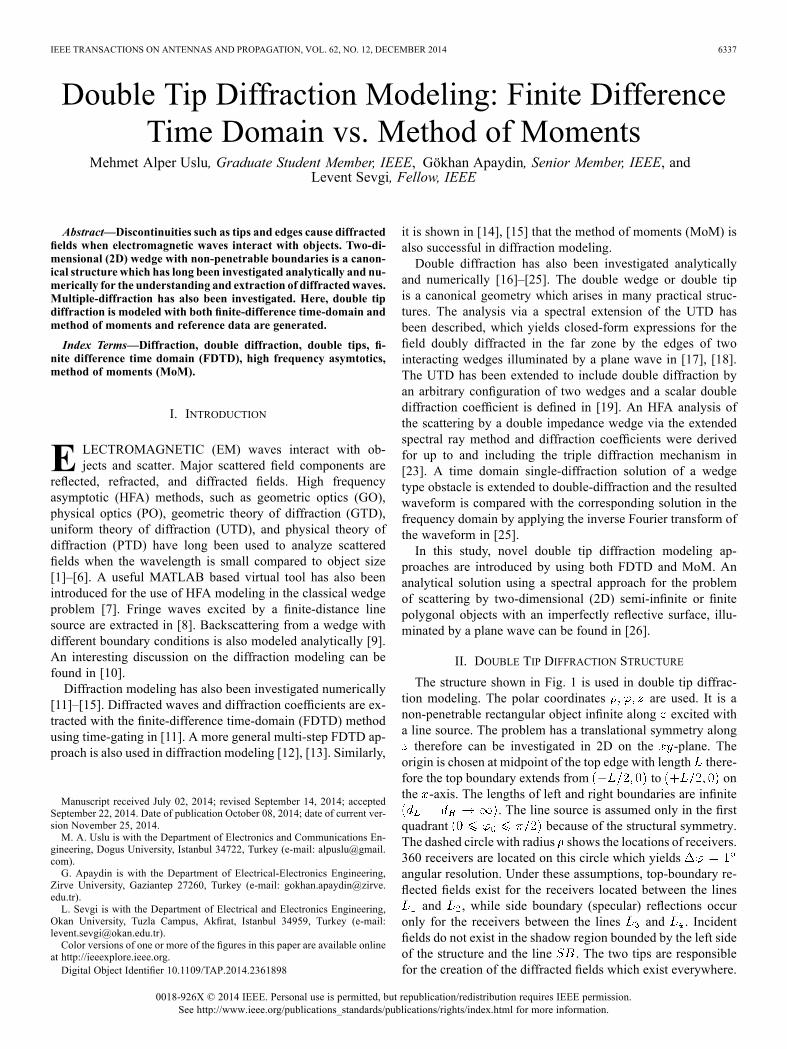
II. DOUBLE TIP DIFFRACTION STRUCTURE

The structure shown in Fig. 1 is used in double tip diffrac-tion modeling. The polar coordinates are used. It is anon-penetrable rectangular object infinite along excited witha line source. The problem has a translational symmetry alongtherefore can be investigated in 2D on the -plane. The

origin is chosen at midpoint of the top edge with length there-fore the top boundary extends from to onthe -axis. The lengths of left and right boundaries are infinite

. The line source is assumed only in the firstquadrant because of the structural symmetry.The dashed circle with radius shows the locations of receivers.360 receivers are located on this circle which yieldsangular resolution. Under these assumptions, top-boundary re-flected fields exist for the receivers located between the lines

and , while side boundary (specular) reflections occuronly for the receivers between the lines and . Incidentfields do not exist in the shadow region bounded by the left sideof the structure and the line . The two tips are responsiblefor the creation of the diffracted fields which exist everywhere.

0018-926X © 2014 IEEE. Personal use is permitted, but republication/redistribution requires IEEE permission.See http://www.ieee.org/publications_standards/publications/rights/index.html for more information.

6338 IEEE TRANSACTIONS ON ANTENNAS AND PROPAGATION, VOL. 62, NO. 12, DECEMBER 2014

Fig. 1. Double tip structure (Structure-1).

Note that Fig. 1 shows the reflection and shadow regions for.

Mathematically, the problem is postulated via the 2D waveequation in polar coordinates

(1)where is the wave-number, is the line current amplitude,

and specify the source and the observationpoints, respectively, is the Dirac delta function. The relatednon-penetrable boundary conditions (BCs) are (TMcase) or (TE case) on the structure. Radiationcondition also applies.In the limit when the lengths of left and right boundaries goes

to zero the structure yields another canonicalscattering problem; the infinite strip problem. This is pictured inFig. 2. The tips marked with number 1 and 2 are responsible forthe creation of the diffracted fields. In this case, reflected fieldsonly exist for the receivers located between the lines and. The region between the lines and is the shadow

region where no incident field exists. The incident, scattered,and diffracted field components all exist elsewhere.Note also that, the structure in Fig. 1 also reduces to (ver-

tical) half-plane problem when meaning that three im-portant canonical problems can be investigated at the same timeonce numerical models are established for the Structure-1 in thefigure.Electromagnetic line source may be the -component of ei-

ther electric field intensity ( , TM case) or magnetic fieldintensity ( , TE case). In the case of acoustic waves,these conditions refer to acoustically soft andhard boundary conditions, respectively.Note that, the word scattering represents all types of waves

generated from EM (incident) wave-object interaction (e.g., re-flections, refractions, diffractions, creeping waves, whisperinggallery waves, etc.). The addition of scattered and incident fieldsyields total fields. Diffractions occur from edge and/or tip typediscontinuities.

Fig. 2. Infinite strip problem (Structure-2).

III. FDTD-BASED DIFFRACTION MODELING

The FDTDmethod is one of themost popular andwidely usedmodels used in electromagnetics [27]. It has been widely usedin variety of EM problems, from radiation, propagation, scat-tering to microstrip circuit design, from subsurface imaging toantenna design, etc. The FDTDmethod has also been used in thecalculation of diffraction coefficients and there are many studiesin modeling diffraction from various wedges [11]–[13]. Notethat, the incident field is a pulse in time therefore broad banddiffraction characteristic can be obtained via a single FDTDsimulation. Once incident and diffracted pulses are recorded,discrete/fast Fourier transform (DFT/FFT) can be applied anddiffraction coefficient vs. frequency and/or diffraction coeffi-cients vs. angle variations can be obtained.The 2D FDTD models used for TM and TE polarizations on

the -plane contain sets of , , and , , com-ponents, respectively. The update equations for polariza-tion and polarization are shown as

(2a)

(2b)

(2c)

(3a)

USLU et al.: DOUBLE TIP DIFFRACTION MODELING: FINITE DIFFERENCE TIME DOMAIN VS. METHOD OF MOMENTS 6339

(3b)

(3c)

The multi-step FDTD approach introduced in [13] is ex-tended here for the calculation of double tip diffractions. Theincident, reflected, and diffracted fields are separated in the timeand then total and/or diffracted fields vs. angle are obtained bythe application of FFT. For the structure in Fig. 1, diffractedfields are extracted with the following 4 steps:1) Run the FDTD simulation with the structure and recordtransient responses at the specified number of receivers onthe observation circle. This will yield total fields.

2) Remove the structure, re-run the FDTD simulation in free-space and record transient responses at the same receivers.This will yield incident fields.

3) Replace the structure with infinite-plane (in other words,extend the top edge of the structure infinitely on the hor-izontal axis) and re-run the FDTD simulations. Recordedfields will include only incident and reflected fields on theupper half plane. Use them only for the receivers locatedbetween the lines and .

4) Extend the right side of the structure infinitely on the ver-tical direction and repeat step 3. Recorded fields will in-clude only incident and reflected fields on the right halfplane. Use them only for the receivers located between thelines and .

Once time variations of the fields for the 4 steps are obtainedincident and reflected fields are extracted in regions where theyexist and only time variations of diffracted fields are left at thereceivers on the observation circle. Diffracted fields at a speci-fied frequency can then be extracted by the application of FFTon all receivers’ data.Note that, only the first 3 steps are enough to extract diffracted

field data for the infinite strip shown in Fig. 2. Moreover, onlythe first 2 steps are enough to obtain scattered field.

IV. MOM-BASED DIFFRACTION MODELING

A similar multi-step MoM is also used in diffraction mod-eling as described in [14], [15]. Here, the method is extended todouble tip diffraction problem.In this model, the three boundaries of Structure-1 in Fig. 1 are

divided into small segments (where segment lengths are muchsmaller than the wavelength). Although , theyhave to be finite in numerical algorithms. Side-boundary lengthsbetween are enough depending on the parametersof the problem at hand. The length of top-boundary is finite.The currents on each segment are assumed to be constant. In

the standard MoM, the source-excited segment fields are calcu-lated, the matrix system is built, and the segment currents arecalculated numerically from the solution of the derived systemof equations [14]. The segment-scattered fields at the observerare then accumulated.Necessary MoM equations (with the time depen-

dence) in this procedure are

(4a)

(4b)

where denotes the field at matching points on eachsegment and the impedance matrix is obtained

(5a)

(5b)

where is the segment length, is the intrinsicimpedance of free space, and are the first kind Hankelfunctions with order zero and one, respectively, is theexponential of the Euler constant, denotes the unit normalvector of the segment at , and is the unit vector in thedirection from source to the receiving element . Whileconsidering the effects of segment currents, the scattered fieldsare

(6a)

(6b)

The MoM procedure is implemented as follows: The fieldsupon segments in (4) are calculated by using the free-spaceGreen’s function. The impedance matrix in (5) is formed. Then,the source-induced segment currents are obtained. Finally, scat-tered fields in (6) on the chosen observation points are calculatedfrom the superposition of segment radiations using the Green’sfunction.The direct wave from the source to the receiver and scattered

waves from all segments to the receiver are added and total waveat the receiver is obtained.For the structure in Fig. 1, MoM computed diffracted fields

are extracted with the following 3 steps:1) Run the MoM simulation with the structure and record thescattered fields at the specified number of receivers on theobservation circle.

2) Replace the structure with infinite-plane (in other words,extend the top edge of the structure infinitely on the hor-izontal axis) and re-run the MoM simulations. Recordedscattered fields will include only reflected fields on the

6340 IEEE TRANSACTIONS ON ANTENNAS AND PROPAGATION, VOL. 62, NO. 12, DECEMBER 2014

Fig. 3. Single and double tip diffractions; (a) single diffraction from right tip,(b) double diffractions from RL-tips, (c) single diffraction from left tip, (d)double diffractions from LR-tips.

upper half plane. Use them only for the receivers locatedbetween the lines and .

3) Extend the right side of the structure infinitely in the ver-tical direction and repeat step 2. Recorded scattered fieldswill include only reflected fields on the right half plane.Use them only for the receivers located between the linesand .

Only the first 2 steps are enough to extract diffracted field datafor the infinite strip (Structure-2) shown in Fig. 2. MoM directlyyields scattered fields therefore only the first step is enough forthe extraction of scattered fields.MATLAB algorithms are developed for both FDTD—and

MoM-based diffraction modeling. The next section presentsseveral comparisons. Note that, diffracted fields presented in thefollowing examples contain single and double tip diffractionsfrom both tips. Fig. 3 illustrates single and double diffractedwaves from the left tip. The right tip also contributes the samesingle and double diffracted waves.Note that, standard free-space FDTD and MoM algorithms

are used here. The FDTD space is terminated with absorbingboundary layers and edges are directly extended into theselayers. This is how infinite length structure issimulated. On the other hand, edges are truncated in MoM sothat and are finite, but the lengths of the truncated edgesare long enough to simulate . One needs tocheck if the first segment beyond the truncation has negligibleinduced current. Beyond the truncation, this (i.e., the simulationof the infinite edges) is achieved if the scattered field at thenearest receiver, caused by the segment currents is less thana specified value corresponding to the stated accuracy and/orerror. Relative accuracy of 1% or less is used to generate all theexamples presented in the next section.

Fig. 4. Total, diffracted, and scattered fields around Structure-1; ,, , , , TM/SBC case, Solid: MoM,

Dashed: FDTD.

V. EXAMPLES AND COMPARISONS

The examples given in this section present total, diffracted,and scattered fields around Structure-1, Structure-2, and for thevertical half-plane for a given line source at 30MHz. Source andobserver radial distances are 100 m and 80 m, respectively. The polarizations and angle of incidences are

mentioned in figure captions.In Fig. 4; total, diffracted, and scattered fields around the tip

of a vertical half-plane, simulated with both FDTD and MoMapproaches, are given. Here, the angle of incidence is .The top side of Structure-1 is taken as . As ob-served in the total field plot, the ripples in the angular region

correspond the interference of incidentand diffracted fields, the ripples in the angular region

correspond the interference of incident, diffracted,and reflected fields. The dominant diffraction occurs along thetwo critical boundaries incident shadow boundary (ISB) and re-flection shadow boundary (RSB). On the other hand, forwardscattering and specular reflections dominate the scattered fields.Figs. 5–7 belong to scattering from Structure-1. Total, dif-

fracted and scattered fields, simulated with both FDTD andMoM approaches for different illumination angles and topsurface lengths are shown in Figs. 5 and 6. Only total anddiffracted fields are given in Fig. 7. Note that, there are twotips and four critical boundaries. The diffracted fields alongthese boundaries and their interference for different top surfacelengths are observed.Figs. 8–10 belong to the FDTD and MoM simulation results

for the Structure-2 (infinite strip). Scattered fields are also in-cluded in Figs. 9 and 10. As observed angular variations of total,scattered, and diffracted fields for different angles of illumina-tion with different top surface lengths, the forward scattering

USLU et al.: DOUBLE TIP DIFFRACTION MODELING: FINITE DIFFERENCE TIME DOMAIN VS. METHOD OF MOMENTS 6341

Fig. 5. Total, diffracted, and scattered fields around Structure-1; ,, , , , TE/HBC case, Solid: MoM, Dashed:

FDTD.

Fig. 6. Total, diffracted, and scattered fields around Structure-1; ,, , , , TM/SBC case, Solid: MoM, Dashed:

FDTD.

and specular reflections dominate the scattering fields, but, asmentioned above, dominant diffractions are observed along crit-ical boundaries. On the other hand, interference of the doublediffractions may change the picture significantly depending onthe angle of illumination and top surface lengths.Note that, different discretizations are required in MoM sim-

ulations for the TM (SBC) and TE (HBC) polarizations. Infinite

Fig. 7. Total (Left) and diffracted (Right) fields around Structure-1; ,, , , , TM/SBC case, Solid: MoM,

Dashed: FDTD.

Fig. 8. Total (Left) and diffracted (Right) fields around Structure-2; ,, , , , TM/SBC case, Solid: MoM,

Dashed: FDTD.

sides of Structure-1 are approximated by 10 -long finite sidesfor the TM polarization. On the other hand, up to 100 -longside-lengths may be required for the TE polarization (becauseill-conditioned matrices may be obtained in this polarization).The segment lengths are chosen to be /20. The FDTD cell sizesare taken as /20.The source is above the horizontal plane in these examples,

but it can be located arbitrarily anywhere in the angular domain.In this case, one has to pay attention to the infinite boundaries inboth FDTD and MoM procedures. In other words, when a plane(or cylindrical) wave of incidence below the horizontal plane isconsidered, the infinite boundaries must extend well beyond thesource.Note also that, there are highly effective commercial FDTD

and MoM packages that can be used in numerical simulationof broad range of EM problems. Unfortunately, they cannot beused in solving the problems discussed in this paper. By usinga commercial package, total fields can be reproduced, but scat-tered and/or diffracted fields cannot be discriminated using themulti-step approach introduced here.

6342 IEEE TRANSACTIONS ON ANTENNAS AND PROPAGATION, VOL. 62, NO. 12, DECEMBER 2014

Fig. 9. Total, diffracted, and scattered fields around Structure-2; ,, , , , TM/SBC case, Solid: MoM, Dashed:

FDTD.

Fig. 10. Total, diffracted, and scattered fields around Structure-2; ,, , , , TM/SBC case, Solid: MoM,

Dashed: FDTD.

VI. CONCLUSION

Double tip diffraction modeling using multi-step FDTD andMoM approaches in 2D is discussed. MATLAB-based diffrac-tion algorithms are developed and numerical results are pre-sented. Very good agreement between the results shows thatboth FDTD and MoM can be used effectively in diffractionmodeling.

The novel multi-step multi-tip diffraction modeling intro-duced here is highly effective for the numerical models suchas FDTD and MoM. Its extension to 3D is straightforward.Since the power and beauty of these numerical models istheir application capability directly in 3D, distinguishing anddiscriminating scattered and diffracted fields for the realisticobjects in 3D would be very helpful in understanding anddesigning low-visible objects.Note that, the reader is referred to [28]–[31] for indoor, ane-

choic chamber measurement results which belong to 2D prop-agation above flat, perfectly reflecting surface with single anddouble diffractive obstacles.

REFERENCES

[1] P. Y. Ufimtsev, Fundamentals of the Physical Theory of Diffraction (inRussian). Hoboken, NJ, USA: Wiley, 2007.

[2] C. A. Balanis, L. Sevgi, and P. Y. Ufimtsev, “Fifty years of high fre-quency diffraction,” Int. J. RF Microw. Comput.-Aided Engrg., vol. 23,no. 4, pp. 394–402, Jul. 2013.

[3] G. Pelosi, Y. Rahmat-Samii, and J. L. Volakis, “High-frequency tech-niques in diffraction theory: 50 years of achievements in GTD, PTD,related approaches,” IEEE Antennas Propag. Mag., vol. 55, no. 4, pp.17–19, Aug. 2013.

[4] P. Y. Ufimtsev, “The 50-year anniversary of the PTD: Comments onthe PTD’s origin and development,” IEEE Antennas Propag.Mag., vol.55, no. 3, pp. 18–28, Jun. 2013.

[5] Y. Rahmat-Samii, “GTD, UTD, UAT, STD: A historical revisit andpersonal observations,” IEEE Antennas Propag. Mag., vol. 55, no. 3,pp. 29–40, Jun. 2013.

[6] G. Pelosi and S. Selleri, “The wedge-type problem: The building brickin high-frequency scattering from complex objects,” IEEE AntennasPropag. Mag., vol. 55, no. 3, pp. 41–58, Jun. 2013.

[7] F. Hacivelioglu, M. A. Uslu, and L. Sevgi, “A Matlab-based virtualtool for the electromagnetic wave scattering from a perfectly reflectingwedge,” IEEE Antennas Propag. Mag., vol. 53, no. 6, pp. 234–243,Dec. 2011.

[8] F. Hacivelioglu, L. Sevgi, and P. Y. Ufimtsev, “Wedge diffractedwavesexcited by a line source: Exact and asymptotic forms of fringe waves,”IEEE Trans. Antennas Propag., vol. 61, no. 9, pp. 4705–4712, Sept.2013.

[9] F. Hacivelioglu, L. Sevgi, and P. Y. Ufimtsev, “Backscattering from asoft-hard strip: Primary edge waves approximations,” IEEE AntennasWireless Propag. Lett., vol. 12, pp. 249–252, 2013.

[10] F. Hacivelioglu, L. Sevgi, and P. Y. Ufimtsev, “On the modified theoryof physical optics,” IEEE Trans. Antennas Propag., vol. 61, no. 12, pp.6115–6119, Dec. 2013.

[11] G. Stratis, V. Anantha, and A. Taflove, “Numerical calculation ofdiffraction coefficients of generic conducting and dielectric wedgesusing FDTD,” IEEE Trans. Antennas Propag., vol. 45, no. 10, pp.1525–1529, Oct. 1997.

[12] G. Cakir, L. Sevgi, and P. Y. Ufimtsev, “FDTD modeling of elec-tromagnetic wave scattering from a wedge with perfectly reflectingboundaries: Comparisons against analytical models and calibration,”IEEE Trans. Antennas Propag., vol. 60, no. 7, pp. 3336–3342, Jul.2012.

[13] M. A. Uslu and L. Sevgi, “Matlab-based virtual wedge scattering toolfor the comparison of high frequency asymptotics and FDTDmethod,”App. Comp. Electromagn. Soc. J., vol. 27, no. 9, pp. 697–705, Sep.2012.

[14] G. Apaydin and L. Sevgi, “A novel wedge diffraction modeling usingmethod of moments,” App. Comp. Electromagn. Soc. J., submitted forpublication.

[15] G. Apaydin, F. Hacivelioglu, L. Sevgi, and P. Y. Ufimtsev, “Wedgediffracted waves excited by a line source: Method of moments (MoM)modeling of fringe waves,” IEEE Trans. Antennas Propag., vol. 62, no.8, pp. 4368–4371, Aug. 2014.

[16] R. Tiberio, G. Manara, G. Pelosi, and R. G. Kouyoumjian, “Scatteringby a strip with 2 face impedances at edge-on incidence,” Radio Sci.,vol. 17, no. 5, pp. 1199–1210, 1982.

[17] R. Tiberio, G. Manara, G. Pelosi, and R. G. Kouyoumjian, “High fre-quency diffraction by a double wedge,” presented at the IEEE Int.Symp. on Antennas Propag., Vancouver, Canada, Jun. 1985.

USLU et al.: DOUBLE TIP DIFFRACTION MODELING: FINITE DIFFERENCE TIME DOMAIN VS. METHOD OF MOMENTS 6343

[18] R. Tiberio, G. Manara, G. Pelosi, and R. G. Kouyoumjian, “High-fre-quency electromagnetic scattering of plane-waves from doublewedges,” IEEE Trans. Antennas Propag., vol. 37, no. 9, pp. 1172–1180,Sep. 1989.

[19] M. Schneider and R. Luebbers, “A general uniform double wedgediffraction coefficient,” IEEE Trans. Antennas Propag., vol. 39, no. 1,pp. 8–14, Jan. 1991.

[20] L. P. Ivrissimtzis and R. J. Marhefka, “A note on double edge-diffrac-tion for parallel wedges,” IEEE Trans. Antennas Propag., vol. 39, no.10, pp. 1532–1537, Oct. 1991.

[21] M. Albani, F. Capolino, S. Maci, and R. Tiberio, “Double diffrac-tion coefficients for source and observer at finite distance for a pairof wedges,” in Proc. IEEE Int. Symp. on Antennas and Propagation,1995, vol. 2, pp. 1352–1352.

[22] F. Capolino and S. Maci, “Uniform high-frequency description ofsingly, doubly, vertex diffracted rays for a plane angular sector,” J.Electromagn. Waves Applicat., vol. 10, no. 9, pp. 1175–1197, Oct.1996.

[23] M. I. Herman and J. L. Volakis, “High-frequency scattering by a doubleimpedance wedge,” IEEE Trans. Antennas Propag., vol. 36, no. 5, pp.664–678, May 1988.

[24] M. Albani, “A uniform double diffraction coefficient for a pair ofwedges in arbitrary configuration,” IEEE Trans. Antennas Propag.,vol. 53, no. 2, pp. 702–710, Feb. 2005.

[25] A. Karousos and C. Tzaras, “Time-domain diffraction for a doublewedge obstruction,” in Proc. IEEE Int. Symp. on Antennas Propag.,Hawaii, Jun. 2007, pp. 4153–4156.

[26] J. M. L. Bernard, “A spectral approach for scattering by impedancepolygons,”Quart. J. Mechan. Appl. Math., vol. 59, no. 4, pp. 517–550,Nov. 2006.

[27] K. S. Yee, “Numerical solution of initial boundary value problemsinvolving Maxwell’s equations in isotropic media,” IEEE Trans. An-tennas Propag., vol. 14, no. 3, pp. 302–307, May 1966.

[28] D. Erricolo, U. G. Crovella, and P. L. E. Uslenghi, “Time-domain anal-ysis of measurements on scaled urban models with comparisons toray-tracing propagation simulation,” IEEE Trans. Antennas Propag.,vol. 50, no. 5, pp. 736–741, May 2002.

[29] D. Erricolo, G. D’Elia, and P. L. E. Uslenghi, “Measurements on scaledmodels of urban environments and comparisons with ray-tracing prop-agation simulation,” IEEE Trans. Antennas Propag., vol. 50, no. 5, pp.727–735, May 2002.

[30] D. Erricolo, “Experimental validation of second order diffraction coef-ficients for computation of path-loss past buildings,” IEEE Trans. Elec-tromagn. Compat., vol. 44, no. 1, pp. 272–273, Feb. 2002.

[31] T. Negishi, V. Picco, D. Spitzer, D. Erricolo, G. Carluccio, F. Puggelli,and M. Albani, “Measurements to validate the UTD triple diffrac-tion coefficient,” IEEE Trans. Antennas Propag., vol. 62, no. 7, pp.3723–3730, Jul. 2014.

Mehmet Alper Uslu (M’14) was born in Turkey,in 1986. He received B.S. and M.S. degrees in elec-tronics and communication engineering from DogusUniversity, Turkey, in 2010 and 2012, respectively,where he is currently working toward the Ph.D.degree.His research interests are diffraction theory, com-

putational electrodynamics, RF Microwave circuitsand systems, EMC and Digital signal processing al-gorithms.Mr. Uslu is one of the two recipients of Dogus Uni-

versity–Felsen Fund Excellence in Electromagnetics 2011 award.

Gökhan Apaydin (M’08–SM’11) received the B.S.,M.S., and Ph.D. degrees in electrical and electronicsengineering from Bogazici University, Istanbul,Turkey, in 2001, 2003, and 2007, respectively.From 2001 to 2005, he was a Teaching and

Research Assistant with Bogazici University. From2005 to 2010, he was a Project and Research Engi-neer with the Applied Research and Development,University of Technology Zurich, Zurich, Switzer-land. Since 2010, he has been with Zirve University,Gaziantep, Turkey. He has been working on several

research projects on analytical and numerical methods (FEM, MoM, FDTD,SSPE) in electromagnetic propagation, radiowave propagation modeling,diffraction modeling, positioning, filter design, waveguides, and related areas.

Levent Sevgi (M’99–SM’02–F’09) received theB.S.E.E., M.S.E.E., and Ph.D. degrees in electronicengineering from Istanbul Technical University(ITU), Istanbul, Turkey, in 1982, 1984, and 1990,respectively. While working on his Ph.D. in 1987 hewas awarded a fellowship that allowed him to workfor two years with Prof. L. B. Felsen at the WeberResearch Institute/New York Polytechnic UniversityYork, Brooklyn, NY, USA.Since September 2014, he has been with the Elec-

trical and Electronics Engineering Department, Fac-ulty of Engineering and Architecture, OkanUniversity. He has beenwith severalinstitutions for the last two decades: Istanbul Technical University (1991–1998),The Scientific and Technological Council of Turkey–Marmara Research Insti-tute (1999–2000), as the Chair of Electronics Systems Department, Weber Re-search Institute/Polytechnic University in New York (1988–1990), the Scien-tific Research Group of Raytheon Systems, Canada (1998–1999) during Cana-dian East Coast Integrated Surveillance System trials, with Center for DefenseStudies, ITUV-SAM (1993–1998) during large scale system designs for TurkishNavy and (2000–2002) during Maritime Vessel Traffic Monitoring System de-sign for Turkish Straights, with Dogus University (2001–2014), and with theDepartment of ECE, UMASS Lowell, MA, USA (2012–2013) for his sabbat-ical term. He has been involved with complex electromagnetic problems andsystems for more than two decades. His research study has focused on analyticaland numerical methods in electromagnetics, high frequency asymptotic (HFA)approaches, FDTD, TLM, FEM, SSPE, and MoM techniques and their applica-tions, propagation in complex environments, diffraction modeling, Microwavecircuit design, EMC/EMI modeling and measurement, sensors and integratedsurveillance systems, surface wave HF radars, RCS modeling and bio-electro-magnetics. He is also interested in novel approaches in engineering educationand popular science topics such as science, technology and society and publicunderstanding of science. He has published many books/book chapters in Eng-lish and Turkish, including the two books Complex Electromagnetic Problemsand Numerical Simulation Approaches (IEEE Press-Wiley, 2003) and Electro-magnetic Modeling and Simulation (IEEE Press-Wiley, 2014), over 150 journal/magazine papers/tutorials, and has attended nearly 100 international confer-ences/symposiums.Prof. Sevgi is a Fellow of the IEEE, Associate Editor of the IEEE Antennas

and Propagation Magazine, and is the writer/editor of the “Testing ourselves”Column, and a member of the IEEE Antennas and Propagation Society AdCom(2013–2015) and Education Committee.