a theory of wage determination - a training model …etheses.lse.ac.uk/1488/1/u109685.pdf · a...
TRANSCRIPT

A THEORY OF WAGE DETERMINATION
- A Training Model with Heterogeneous Labour Approach -
Yasushi Tanaka
Ph.D, LSE

UMI Number: U109685
All rights reserved
INFORMATION TO ALL USERS The quality of this reproduction is dependent upon the quality of the copy submitted.
In the unlikely event that the author did not send a com plete manuscript and there are missing pages, th ese will be noted. Also, if material had to be removed,
a note will indicate the deletion.
Dissertation Publishing
UMI U109685Published by ProQuest LLC 2014. Copyright in the Dissertation held by the Author.
Microform Edition © ProQuest LLC.All rights reserved. This work is protected against
unauthorized copying under Title 17, United States Code.
ProQuest LLC 789 East Eisenhower Parkway
P.O. Box 1346 Ann Arbor, Ml 48106-1346

T\^s^s
f
7/ffcS
biziuz
ABSTRACT
This thesis offers an alternative approach to the theory of wage determination, producing new and interesting interpretations to labour market phenomena. Based on the assumption of heterogeneous labour, a training model based on the concept of adverse selection is introduced. The unique feature of this model is that the heterogeneity is expressed in terms of the cost of OJT as well as the opportunity wage of the potential workers. The model suggests that the existence of unemployment and the downward wage rigidity are conditional upon the market characteristics and that the unemployment can not be eliminated by lowering the wage. It also suggests that policies to control the demand side of the market such as accepting of immigration of able workers, raising the educational standard of the domestic workers, or subsidizing the firm's OJT would be more effective.
Also as a training model, the analysis includes a two-period model, in which the upward-sloping wage profile is derived.
The analysis is extended to the idea of multiple wage equilibrium in one market, which in turn offers a new dimension to the analysis of income distribution. One important result here is that whatever happens in the society will first affect the weakest, to whom therefore the policy makers need to pay greater attention. The derivation of a skewed distribution of wage offers yet one more explanation to the Pigou paradox.
The model attempts also to explain how firms choose workers in the real world job offers usually states a minimum hiring standard as well as the offer wage, and how they react to economic fluctuations — would they, for example, reduce the wage or raise the minimum hiring standard when the demand for the product falls. The analysis suggests that the weaker members of the society are more prone to exogeneous shocks.

CONTENTS
CHAPTER I : INTRODUCTION.............................................................................. 6(1) Efficiency Wage Hypothesis............................................................................7(2) Adverse Selection Model of Labour Market................................................ 12(3) Limitations of the EWH Models.................................................................... 16(4) Thurow’s Job Competition Model................................................................. 25(5) Towards a More General Model of a Labour Market..................................27
CHAPTER I I : A SURVEY OF LITERATURE ON THEORIES OF WAGE DETERMINATION...................................................................................................36
(1) The Overall V iew ............................................................................................ 36(2) The Theories .................................................................................................. 39(3) Training Models of a Labour M arket........................................................... 55(4) Towards the Training Model of Heterogeneous Labour Market............... 68
CHAPTER I I I : THE M ODEL................................................................................ 72(1) Assumptions.....................................................................................................74(2) The Model.........................................................................................................76(3) Equilibrium.......................................................................................................85
CHAPTER IV : THE VALIDITY OF UNIFORM WAGE................................. 94(1) Possible Reasons for the Uniform Wage : the Weiss Model......................95(2) Uniform Wage and OJT.................................................................................. 97(3) Pooling Equilibrium and Its Robustness...................................................... 98(4) An Application to the Case Where Ability Is Continuous....................... 110
CHAPTER V : TWO-PERIOD MODELS...........................................................114(1) The Basic Framework................................................................................... 114(2) Case I : Optimizing At Each Period............................................................117(3) Case I I : Optimizing Over Two Periods..................................................... 120
-3 -

CHAPTER V I : MONOPSONY AND COMPETITION IN HETEROGENEOUS LABOUR MARKETS...................................................... 135
(1) The Lagrangian and the Constraints............................................................136(2) The Cases........................................................................................................138
CHAPTER V II : COMPARATIVE STATICS.................................................... 146(1) The Functions................................................................................................ 147(2) Comparative Statics.......................................................................................155(3) Policy Implications........................................................................................161
CHAPTER V III : HETEROGENEOUS FIRMS.................................................168(1) Equilibrium.................................................................................................... 168(2) Training Cost Function and Multiple Wage Equilibrium......................... 177(3) Comparative Statics.......................................................................................178(5) Statistical Discrimination.............................................................................185(6) Policy Implications........................................................................................186
CHAPTER IX : OBSERVATIONALLY DISTINGUISHABLE WORKERS.......................................................................................................................................190
(1) Introduction ......................................................................................190(2) The Model.......................................................................................................195(3) Comparative Statics ........................................................................... 200(4) Policy Implications....................................................................................... 211
CHAPTER X : CONCLUSION............................................................................ 215
BIBLIOGRAPHY 221

ACKNOWLEDGEMENTS
I am indebted to many people, without whose suggestions, encouragement and patience this thesis would not have been completed.
Firstly the greatest debt is due to Frank A. Cowell, who has provided me in the beginning with the original idea and throughout the process with many suggestions for corrections and improvements, and above all has spared me his great patience.
Secondly, discussions with a following list of people were invaluable not only as contributions to my thesis but also for my better understanding of economics as a whole. Without them I would probably not have appreciated and enjoyed this discipline in such a great depth. This list must include, but in no particular order, Michio Morishima, Oliver Hart, John Moore, Keiichiro Obi, Takamitsu Sawa, Haruo Shimada, Masahiro Okuno, Yusaku Kataoka, Haruo Imai, Jun Iritani, Yoshio Higuchi. It goes without saying, however, that all responsibility for errors lies with the author.
I would also like to thank the Economic Department at London School of Economics and the Faculty of Economics at Kyoto Sangyo University for their kindness in allowing me to use their facilities.
Finally, for her support in forms of constant encouragement and patience I owe an irredeemable debt to my wife, Mari-cruz.
CHAPTER I : INTRODUCTION
Traditional analyses of the labour market, in which the equilibrium is achieved
when the supply equals the demand at a certain wage level, invariably have two
apparent implications among others: i) there exists no involuntary unemploy
ment and ii) the wage paid for a given grade of labour is uniform. The validity
of the first has been a focus of discussion for some time and in great depth, as
every economist would know. And among these are a significant number of
attempts by Neo-classical economists to explain what should be described as a
discrepancy between this Neo-classical implication and the reality that tends to
support the existence of involuntary unemployment (See, for example, Clower
(1965), and Barro & Grossman (1971)).
However, there have been few discussions as to why a uniform wage should be
paid within the competitive market framework, despite the fact that workers are
not necessarily identical even within a single market. The idea behind it is that
labour service offered to perform the job in question is assumed to be homoge
neous, which is a quite separate issue from whether the workers themselves are
homogeneous. Hence, on one hand, the workers may be paid differently in an
alternative job, due to their heterogeneous productivity — this makes aggregate
labour supply upward-sloping. On the other hand, the uniform wage would be
paid to all workers, as they perform identically what they are asked to do. And
there is nothing new in this argument. Simply, we need to add that homoge-
-6 -

neous labour service and heterogeneous labour force are compatible.
But if workers are really identical with respect to the job in question, for
which a uniform wage is paid, how can we possibly explain the very common
phenomenon of employers having clear preference over potential workers?
Given that employers' decisions are rational, it must be that some workers are
more beneficial to the employers than other workers. The offer of a uniform
wage to a heterogeneous labour force suggests that such an offer is made not
because of the homogeneity of their labour service but because of a lack of
information to employers due to its high costs, for example, about the heter
ogeneity of the labour force when offering wages.
(1) The Efficiency Wage Hypothesis
This type of an alternative model of labour market has been developed often
under the name of the "Efficiency Wage Hypothesis". The fundamental feature
of the hypothesis is that, with every worker endowed with some Efficiency
Units (EUs), a level of wage offer affects the EU's of workers in production.
This concept could already be found in the early literature of economics. For
example, Adam Smith wrote:
"The wages of labour are the encouragement of industry, which, like
every other human quality, improves in proportion to the encourage
ment it receives. A plentiful subsistence increases the bodily strength
-7 -

of the labourer, and the comfortable hope of bettering his condition,
and of ending his days perhaps in ease and plenty, animates him to
exert that strength to the utmost. Where wages are high, accordingly,
we shall always find the workmen more active, diligent, and expedi
tious than where they are lo w ”, A.Smith 'Wealth of Nations'(1776)
(p. 184 in reprinted Smith (1977))
In other words, he argued that a higher wage could cause higher productivity
through higher morale and better nutrition. In the current literature there are
several types of models based on the efficiency wage hypothesis, known as the
efficiency wage models. Here we group the main models into four types and
introduce them briefly in turn.
(a) The Nutritional Model
This is the original type of the efficiency wage model. The concept may be
found as early as in the writing of Adam Smith, as pointed out above. The basic
idea is that a higher wage allows a greater level of nutritional intake, which in
turn makes a worker more productive. Attention was more recently drawn to
the concept by Leibenstein (1957), when he discussed about a case of develop
ing economies and it was further developed into more rigorous analyses by
Mirrlees (1975) and Stiglitz (1976). It goes without saying that labour produc
tivity is expressed in terms of efficiency units for this type of model.
(b) The Shirking Model (or The Incentive Model)
-8 -
With this type of model, a worker is assumed to be able to control the amount
of EU to exert in production — the EU input would be small if he shirks or he is
not motivated to work and vice versa. His employer, on the other hand, being
unable to directly control the workers' EU input i.e. the effort, uses the wage
offer as the indirect control device. "Moral hazard" or "Principal-and-Agent
problem" is the terminology given to this kind of situation, which is not con
fined to labour markets. This type of efficiency wage model can be found in
Bowles (1981) & (1983), Calvo (1979), or Shapiro & Stiglitz (1982). The
labour turnover model, as found in Salop (1979) or Stiglitz (1974), may also be
included in this category. In this model a wage offer by a firm is set above the
market-clearing wage in order to reduce labour turnover. As turnover is an act
of lost incentive to work at the workplace, it is equivalent to full shirking.
Consequently, the model can be thought of as having basically the same formal
structure as the shirking model.
(c) The Adverse Selection Model
This type of model is found in Stiglitz (1976), Weiss (1980), or Malcomson
(1981). Unlike the nutritional model or the shirking model, the efficiency unit
endowment of every worker is fixed in the adverse selection model. Given a
heterogeneous work force in terms of efficiency unit endowment, the wage level
determines the composition of the workers willing to work — a higher wage
attracts better workers, i.e. workers with a greater efficiency unit endowment
and vice versa. Note that the heterogeneity of workers is a necessary assump
tion of this model, while in the previous two types of models the work force
-9 -
does not have to be heterogeneous.
(d) Sociological Model
Akerlof (1982) argues that each worker's effort is determined by the work
norms of his work group rather than as a result of neo-classical individual utility
maximization. The model is a sociological one in that it calls for social conven
tions to explain phenomena which seem inexplicable in neo-classical terms.
The common result of all the efficiency wage models is that at the equilibrium
the market may not clear— in fact the equilibrium wage can be higher than the
market-clearing wage, implying an excess supply of labour. This also causes
wage rigidity, when the market faces a change in demand for labour. It is
crucial to the analysis that the endowment of each worker is not known ex-ante
to the employer. If the endowments were known, then the marginal productivi
ty of an efficiency unit (M P^) would be equated to a wage per efficiency unit
(Wgj) at the equilibrium and thus the workers would be paid proportionally to
their EU endowments, resulting in differentiated wages. The analysis then
would not differ much from our usual Neo-classical analysis, except for replac
ing "labour" by "efficiency unit". And in particular there would be market
clearing in terms of supply of and demand for efficiency units. Indeed, the
efficiency wage models base their distinctive results on an assumption that the
efficiency units actually exerted in production is unobservable. This would
mean, for example, that the effort is unobservable in the shirking model or that
the workers are indistinguishable in the adverse selection model. This latter
-10-

assumption clearly needs some justification. (See Chapter IV for extended
discussions on this point)
A higher wage offer attracts a group of workers of better quality "on the
whole" (i.e. of a larger expected efficiency unit endowments). Firms, then, may
choose not to lower the wage when it is faced to an excess supply of labour,
since doing so will lower the expected efficiency unit endowment of the work
ers and may well lower the profit by a reduction in output level. It turns out that
the optimal wage, to be called the Efficiency Wage, is the wage level which
minimizes the labour cost per efficiency unit (See, for, example, Malcomson
(1981)).
The idea of price affecting the quality as well as quantity of the traded good
can be found in other markets, too. Stiglitz & Weiss (1981) point out that the
interest rate a bank charges may itself affect the riskiness of the pool of loans by
either 1) an adverse selection effect, sorting potential borrowers or 2) an incen
tive effect, affecting the actions of borrowers. And it goes without saying that
their two types of effects are analogous to the adverse selection model and the
shirking model of labour market respectively.
This concept of quality dependence on price, though not an established one in
the modem economic theory as a standard assumption, is well-supported by
various observations in the real world not confined only to these two markets.
One may purchase a second-hand car from a well-established firm for a higher
-1 1 -

price rather than from an unknown firm offering a lower price, because he
expects that the former sells a second-hand car of a better quality — this would
be an example of the adverse selection mechanism, or because he expects that
the after-sales services by the former is better — this would be an example of the
incentive mechanism. In both cases the consumer's choice does not depend
solely on the price but also on other conditions of the purchase, i.e. consumers
may not always choose the cheapest good even as a result of rational behaviour.
Typically the dependence of quality on price takes place when the goods are
heterogeneous and yet the heterogeneity can not be perceived accurately or at a
low cost before trading occurs.
Let us now go back to the original question as to why employers have a clear
preference amongst workers. To explain this, we require the labour force to be
heterogeneous, for if workers were truly homogeneous the choice amongst them
would be at random. Of course, what matters here is the perception of the
workers by the firms rather than whether the labour force is indeed heter
ogeneous. However, we appeal to a rational expectations argument that the
firms' perceptions are basically correct. Although all of the efficiency wage
models illustrated above can incorporate the heterogeneity of the labour force,
the adverse selection model is the one that illustrates the issue most clearly for
the heterogeneity is the necessary assumption of the model. So we proceed our
discussion with this type of the efficiency wage model.
(2) The Adverse Selection Model of the Labour Market
-12-
To illustrate the efficiency wage model in a little more rigorous manner, let us
consider a model of Weiss (1980).
Each worker is endowed with labour endowment 0, which determines his
reservation wage — the reservation wage w is derived from one's marginal
productivity in an alternative job. A representative firm, being competitive,
can not control the supply of labour but knows a functional relationship 0=q(w)
and a distribution function of the workers in terms of w, F(w). Although it has
this information on the workers, the firm may be defined as competitive to the
extent that they compete using a wage offer and a volume of labour input (See
Stiglitz & Weiss (1981)).
The firm is assumed to maximize its expected profit n
7i = pg(L)-wx (1-1)
where p is the product price
w is the wage
x is the labour input in terms of number of workers
g(*) is the production function, whose sole input is EU
L is the total number of EU
L, the total amount of EU, is a function of w and we can write it as,
-13 -
L = q(w)x (1-2)
q(z)dF(z)
where q(w)= J0 mVJ---------- (1-3)
dF(z)
/ .
In words, L, the total number of EU, is a product of x, the number of workers
employed and q(w), the expected EU endowment of those workers willing to
work at a wage offer w.
Note that adverse selection implies
q'(w)>0 (1-4)
i.e. the average quality of labour, in terms of EU endowment, rises with the
wage rate.
Maximizing (1-1) w.r.t. w and x, we obtain the following set of equations.
pg'(L)q'(w) = 1 (1-5)
pg'(L)q(w) = w (1-6)
from which we obtain the third equation
-14-

which is also the solution to a problem "min w/q(w)" i.e. "minimize wage per
EU" when its interior solution exists. And this is where the name of the hypoth
esis — the efficiency wage hypothesis — comes from.
Note that w*, the efficiency wage (EW), is derived solely from (1-7), indepen
dent of x*, the employment level. The solution set (w*, x*) of the profit max
imizing problem does not give us a conventional demand schedule of the market
where, to each employment level, there is a corresponding wage when it is
aggregated over all the firms. This also implies that market clearing is not a
necessary condition for the market equilibrium — as long as the quantity de
manded is no greater than the quantity supplied, the equilibrium wage and
employment level of each firm will be established from (1-6) and (1-7) above.
In other words, an equilibrium may be derived, that is locally independent of
the supply condition.
Thus equilibrium is characterized either by excess supply or by market clear
ing, the former presenting a persistent job queue. There will be no "excess
demand" equilibrium since when the demanders find that their demand is not
satisfied, competition will drive up the wage until all the demand is met. Fur
thermore, no worker will acquire a job by compromising to lower his wage
offer, since this would merely single him out as a below-average worker among
those willing to work at that wage.
(3) Theoretical Difficulties and Limitations of the Efficiency Wage Models
As we have seen, the efficiency wage models in general have intuitively
appealing features. However, there are some theoretical difficulties and
limitations related to the models. Some of the extensive arguments on the
theoretical difficulties are found in Akerlof & Yellen (1986) and Weiss (1991).
Here I illustrate their arguments briefly.
For those efficiency wage models in which the workers’ effort levels are the
missing information to the employer, a low wage at the initial apprenticeship
period (Carmichael (1985)), or either a bond payment (Becker & Stigler (1974))
or an employment fee (Eaton & White (1982)) at the beginning of the contract
might act to eliminate the involuntary unemployment. What is common here is
the idea that the workers are paid below their marginal productivity in the initial
period but there will be an compensation in the next period, which acts to
stimulate the incentives of the workers. As a consequence, the offer of an
efficiency wag above the market clearing wage to increase the workers’ effort
becomes redundant. The concept can also be applied to explain the rationale for
the use of seniority wage or the reason why the age-earnings profile is upward-
sloping.(Lazear (1979) & (1981))
The validity of the adverse selection models depends crucially on the
assumption that the firm never finds out about the ability of each worker. If the
-16-

firm did, it could then pay the workers by piece rate. It has also been suggested
that a firm might devise a self-selection scheme or a screening scheme (Guasch
& Weiss (1980), (1981), or (1982)) to differentiate the heterogeneous workers.
However, the real world employment contracts are not always characterized by
a performance bond, an employment fee, or a piece rate, or some type of self
selection or screening scheme. There are several reasons for this. First, with an
imperfect capital market the underpayment in the initial period would not make
the labour market efficient — it is more likely to give a favourable treatment to
those with wealth rather than selecting more productive workers. Second, it is
not easy to measure the precise level of productivity and thus to derive the
corresponding wage that both the employer and the workers accept. When there
is a disagreement between the agents, it is said that there is positive
“transactions cost”, which is the cost of agreeing with each other. And finally, a
well-constructed self-selection or screening devise may be too complicated for
the workers to comprehend or too costly to operate for the employer. A more
formal discussion on this last issue about screening with cost is found in
Chapter IV. While most of these arguments are descriptive rather than
presented within a theoretical framework, their basic arguments do offer
sufficient defence for the efficiency wage models.
The efficiency wage models are based on the concept of efficiency units. But
this fundamental concept itself limits a scope of the models. Here we illustrate
the limitations within the framework of the Weiss model presented in the
-17-

previous section. Weiss (1980) states in the introduction that the existences of
job queues and wage rigidity can be explained if two critical assumptions are
made : (1) The wage received by workers are not proportional to their
productivity, i.e. a uniform wage is paid to workers of heterogeneous
productivity, and (2) the acceptance wages of workers are an increasing
function of their productivity — this also means its inverse exists. While we
leave the discussion on (1) to Chapter IV, consider the validity of (2). There are
at least three limitations brought about by this fundamental assumption of the
efficiency wage model.
Firstly, there is only one efficiency wage for all sorts of labour markets. The
efficiency wage is derived from (1-7), which is a composite function of q(w),
the functional relationship between the labour endowment and the reservation
wage, and F(w), the distribution of workers by the reservation wage but indepen
dent of g(L), the production function. This means that there is a unique efficien
cy wage for all markets, if the idiosyncratic aspect of a particular labour market
in this framework is expressed in terms of g(L). On one hand, to be fair to the
efficiency unit framework, its original intention probably was not meant to
extend the analysis to cover several labour markets. On the other hand, it would
be a useful extension to the model if we can somehow relate the level of efficien
cy wage and the type of labour market. One might attempt to do this by allow
ing the form of 0=q(w) to vary for each labour market so that, for example, the
function for skilled labour market is different from that for unskilled labour
market, resulting in different efficiency wages. However, this would be theoret-
-18-
ical incorrect, as 0 is by definition a parameter attached to each worker rather
than to each labour market.
The second limitation has to do with the existence of the efficiency wage.
Many of the efficiency wage models seem to assume often implicitly that the
efficiency wage always exists. However, it is not necessarily the case. The
equilibrium condition (1-7) is also known as the Solow condition, where the
elasticity of the average labour endowment with respect to wage is unity, since
rearranging (1-7) gives,
dq(w) w r =l . (1-7)
dw q
And as the only assumption concerning q(w) is the adverse selection condition
(1-4), the efficiency wage model does not guarantee the existence of an efficien
cy wage, let alone the excess supply on the wage rigidity.
Fig.I--l(a) supplements the argument. The minimand w/q(w) is an inverse of a
slope of a line through the origin to a point w* on q(w). The function q(w) is
drawn here to have a "convex-concave" shape. Mathematical reason for this is
not difficult to see. Firstly, the second order condition for min {w/q(w)} is
d2/d2w{w/q(w)}=d/dw{(q(w))'2[q(w)-wq’ (w)]}=(q(w))'2{-w(q’,(w)}
Thus the second order condition dictates that it is concave at w*. And the
-19-

concavity for smaller values of w ensures that the solution does not degenerate
to zero.
However, for the efficiency wage to be economically meaningful, these condi
tions have to be justified in economic terms. Noting that q(w) is a composite
function of q(w) and f(w), it is easier to consider the effects of these two compo
nents separately. We may assume that q(w) is a monotonically increasing
function, as it is the inverse of w(0), the reservation wage function, and thus it is
not likely to generate the convex-concave shape alone. As for the frequency
distribution f(w), we may assume it "bell-shaped", with both ends of the distribu
tion having low frequency values. Then, for a given form of q(#), as the pop
ulation is sparse around the both tails, q(w) does not increase at the very low
and very high values of w as much as around the middle range. This would
generate the convexity for the smaller values and the concavity for the larger
values of w in q(*). Alternatively, there may exist a positive value of w, w0, say,
below which no worker is attracted — such as an initial expense for starting out
a new life. This is indicated in Fig.I-l(b) by zero average quality until w0. The
concavity to follow can be explained as the result of the quality of labour eventu
ally approaching some upper bound.
Fig.I-l(c) illustrates a special case where the average quality is invariant across
the workers with different acceptance wages. This can be considered as a case
of "homogeneous" labour force with respect to the job in the market. Note that
the kink at w0=0 of this function helps to maintain the "convexity-concavity"
-20-

characteristics required of q(*). Note that in these realistic cases their character
istics is of a weaker version, i.e. "weak-convexity/weak-concavity". Although
the case of Fig.I-1(c) does not accord with the standard first order derivative
conditions for minimizing w/q(w), the wage may still be defined as an efficien
cy wage in that it is the solution to the minimization problem.
q(w) q(w) q(w)
(b)(a) (c)
Fig.I-1
Of course, more complex shapes are possible. However, as far as the existence
of an efficiency wage is concerned, the "concave-convex" shape is a sufficient
condition. While the existence of an efficiency wage may be justified, there is
no reason to leave out a possibility that an efficiency wage does not exist.
Indeed, in theory if the function were convex (concave) throughout, the objec
tive function would be minimized at w=0 ( at the maximum value of w). How
ever, the economic interpretation presented above in on the shape of q(w) is too
convincing to consider the case that an efficiency wage does not exists. This
argument suggests that the adverse selection models usually analyze the special
cases where the existence of an efficiency wage is the necessary consequence of- 21 -

the adverse selection mechanism.
Thirdly, the adverse selection does not require a one-to-one functional relation
ship between w and 0, which is the consequence of the assumption of efficiency
units (EUs). This, together with a production function g(*) being cumulative in
EU, leads to a situation of "all-round productive ability" among jobs i.e. if a
worker has a higher 0 than another worker then he is more productive in al[
jobs. This, however, is not a necessary condition for an adverse selection
mechanism nor for excess supply equilibrium to occur. For the adverse selec
tion phenomenon implies,
q'(w)>0 and not q'(w)>0 (1-8)
It is easy to give an example where q(w) is an increasing function of w while
q(w) is not. Consider, for example, a discrete case with three workers whose
opportunity wages are w,<w2<w3, and q(w,)=l q(w2)=5 and q(w3)=4. In this
case, q'(w) is an increasing function of w as q(w,)=q(w,)=l, q(w2)=(l/2)
{q(w1)+q(w2)}=3, and q(w3)=(l/3){q(w,)+q(w2)+q(w3)}=10/3, while q(w) is
not. In fact the condition that q(w) and q(w) are both increasing in w is ap
propriate for the early efficiency wage models where an increase in w means an
increase in the productivity of everyone in the homogeneous labour force since
in this case q(w) = q(w). Therefore, for the adverse selection model, the assump
tion that w(0) is monotionic is not an economic argument but is a technical one
in a sense that without this its inverse q(w) may not be defined and this would
-22-
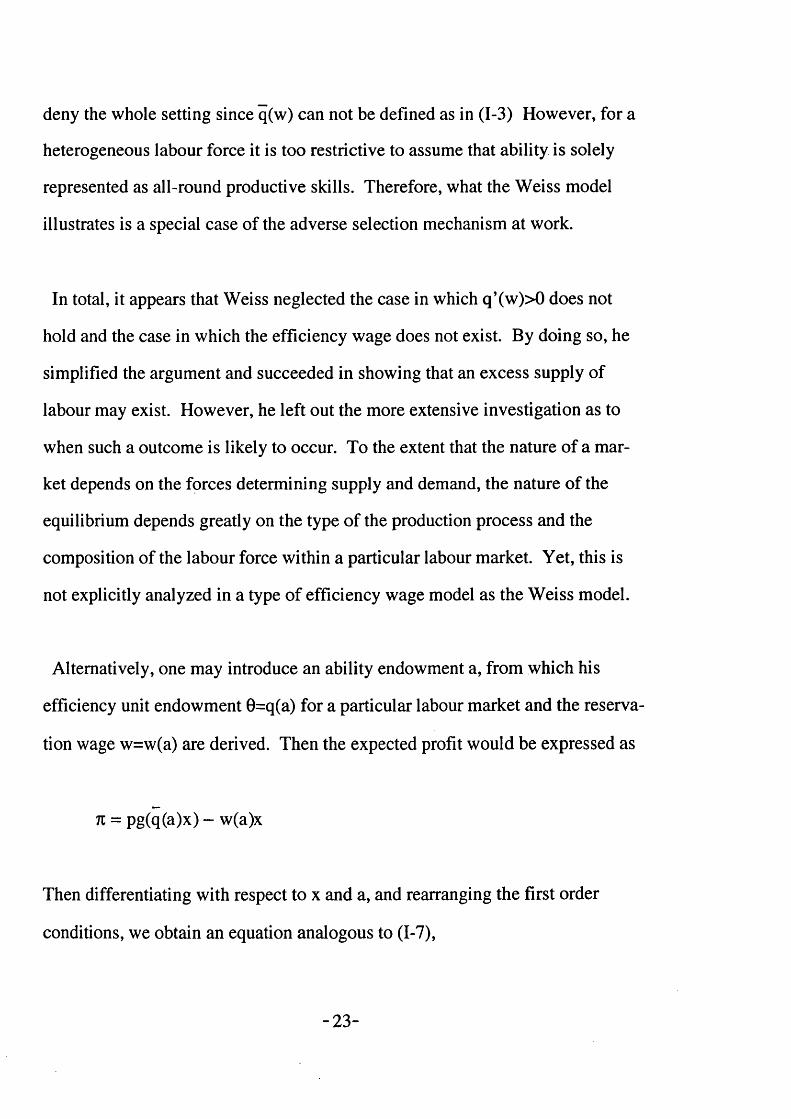
deny the whole setting since q(w) can not be defined as in (1-3) However, for a
heterogeneous labour force it is too restrictive to assume that ability is solely
represented as all-round productive skills. Therefore, what the Weiss model
illustrates is a special case of the adverse selection mechanism at work.
In total, it appears that Weiss neglected the case in which q ’(w)>0 does not
hold and the case in which the efficiency wage does not exist. By doing so, he
simplified the argument and succeeded in showing that an excess supply of
labour may exist. However, he left out the more extensive investigation as to
when such a outcome is likely to occur. To the extent that the nature of a mar
ket depends on the forces determining supply and demand, the nature of the
equilibrium depends greatly on the type of the production process and the
composition of the labour force within a particular labour market. Yet, this is
not explicitly analyzed in a type of efficiency wage model as the Weiss model.
Alternatively, one may introduce an ability endowment a, from which his
efficiency unit endowment 0=q(a) for a particular labour market and the reserva
tion wage w=w(a) are derived. Then the expected profit would be expressed as
n - Pg(q(a)x) - w(a)x
Then differentiating with respect to x and a, and rearranging the first order
conditions, we obtain an equation analogous to (1-7),
-23 -

w(a) w' (a)q(a) q '(a)
and this is also the solution to the analogous problem “min w(a)/q(a)”. Thus the
efficiency wage may depend on the characteristics of the function q(a), which
takes an idiosyncratic form of a particular labour market. This is a possible
extension to the efficiency wage models but is not suggested in the literature —
in fact, Weiss (1991) considers different q(w)’s but they are for different co
horts rather than for different labour markets. This is probably because such an
extension would make the model unnecessarily complicated and the model
could lose its intuitively appealing features.
Table 1-1 summarizes the three limitations : (1) q’(w)>0, the all-round produc
tive ability — this is not a critical assumption for the adverse selection mech
anism, (2) The adverse selection q’(w)>0 implies an existence of an efficiency
wage — this is not necessarily true, and (3) The efficiency wage is invariant
across all jobs — this would treat all the labour markets in the same way so that
we can not analyse the nature of the equilibrium in terms of the market charac
teristics. While the efficiency wage models can claim success in showing that
an excess supply is consistent with competitive equilibrium, there is a need to
The Weiss Model
q ’(w)>0 -> q ’(w)>0 3 Efficiency Wage—> Excess supply or Market Clearing(1) (2) (3)
Table 1-1
-24-
set up a model that can pick up those aspects of the heterogeneous labour mar
ket analysis which the efficiency wage models have not dealt with.
(4) Thurow’s Job Competition Model
Discrepancies that exist between what the economic theory predicts and what
we observe in the real world were the starting point of the analysis of labour
market in Thurow (1975). For him these “deviant observations” in the labour
market included the existence of unemployment and the consequent wage
rigidity, the Pigou paradox, the phenomenon that the distribution of earnings is
skewed despite the allegedly normally distributed abiliiy distribution, and the
observation that the wage payments are not always equalized for homogeneous
labour.
He introduced a concept of “job competition” to explain these deviant observa
tions in a theoretically acceptable manner. As these concerns of his overlap
with our interest, let us briefly introduce his job competition here. The basic
premise of the idea is that labour markets are essentially training markets in the
sense that firms recruit workers in a labour market to train them to perform the
required job. This contrasts with a more orthodox concept of labour market that
workers bring with them the required skills.
In the job competition model, therefore, workers are allocated into job slots
and wages are paid according to the job characteristics rather than the worker’s
-25-
personal characteristics. Furthermore, Thurow’s workers are assumed to be
heterogeneous as opposed to the usual assumption of homogeneous labour force
in the neo-classical model. Thus after recruiting the heterogeneous workers, the
firm offers training to standardize the labour force so that they can all perform
the required job. The workers’ heterogeneity is reflected in their ability to
complete the training — some workers find the training easier than others and
thus they may cost less to train to the firm. As a result, the firms have prefer
ence about the workers and rank them in order of the preference to form a
“labour queue” using educational credentials as a screening device. The prefer
ence about workers do exist also for Weiss (1980). However, his preferred
workers are endowed with more efficiency units, while Thurow preferred
workers have lower training cost than the less preferred ones. Furthermore,
unlike in a neo-classical model of a labour market, the wage in the job competi
tion model is determined outside of the market rather than by the supply and
demand interaction. And this explains the deviant observations of wage rigidity
and unemployment.
The crucial assumption in the Thurow’s model is that the training cost is paid
by the training firm — otherwise, the firm would be indifferent about the work
ers even if they are heterogeneous. The incidence of training cost was discussed
earlier on in Becker (1964), in which he distinguished “general” and “specific”
training. General training is relevant to all jobs and thus acquiring such skill
would increase the productivity of the trainee by exactly the same amount in the
training firm and in other firms, while specific training has relevance only to the
-26-

job of the training firm and the productivity of the trainee in other firms does
not change. Consequently, the Thurow’s training firm would pay for the train
ing since it is specific and not general.
Thurow (1975) contrasts the job competition model with what he calls the
wage competition model. In the latter, firms do not have preference about the
workers even if they are heterogeneous, since the training are general and thus
the cost does not incur to the training firm. These two types of competitions
co-exist in the real world according to Thurow. The way Thurow incorporates
the human investment aspect into the labour market mechanism is rather intrigu
ing. The firm pays to train the workers, and as the workers are heterogeneous in
the training cost the firm has a preference among the workers. This means that
the characteristics of a job competition of a particular labour market depend on
the training cost heterogeneity — for example, if the training cost is uniform,
then the firm will be indifferent about the workers. However, Thurow does not
offer a theoretical model of a job competition nor does he explain how the wage
is determined. This is our starting point and we use the Thurow’s concept of
training market to build a more theoretically rigorous model.
(5) Towards a More General Model of Labour Market
The labour service has a very high degree of heterogeneity, while many types
of goods and services are supplied in relatively homogeneous forms. Hence, it
would be difficult to find two workers with exactly the same level of productivi-
-27 -

job of the training firm and the productivity of the trainee in other firms does
not change. Consequently, the Thurow’s training firm would pay for the train
ing since it is specific and not general.
Thurow (1975) contrasts the job competition model with what he calls the
wage competition model. In the latter, firms do not have preference about the
workers even if they are heterogeneous, since the training are general and thus
the cost does not incur to the training firm. These two types of competitions
co-exist in the real world according to Thurow. The way Thurow incorporates
the human investment aspect into the labour market mechanism is rather intrigu
ing. The firm pays to train the workers, and as the workers are heterogeneous in
the training cost the firm has a preference among the workers. This means that
the characteristics of a job competition of a particular labour market depend on
the training cost heterogeneity — for example, if the training cost is uniform,
then the firm will be indifferent about the workers. However, Thurow does not
offer a theoretical model of a job competition nor does he explain how the wage
is determined. This is our starting point and we use the Thurow’s concept of
training market to build a more theoretically rigorous model.
(5) Towards a More General Model of Labour Market
The labour service has a very high degree of heterogeneity, while many types
of goods and services are supplied in relatively homogeneous forms. Hence, it
would be difficult to find two workers with exactly the same level of productivi-
-27-

ty, while you can find many pencils, say, of the same quality. The reason is
simply that while the quality of labour service depends a lot on the characteris
tics of each individual worker (Nobody is bom identical to anyone else!), many
goods and services are produced as homogeneous products (which makes the
production easier). However, once labour service is to be used as a factor of
production it requires a certain level of homogeneity. In that sense acquiring of
knowledge and skills helps to standardize the innately heterogeneous labour
force. The simplest example of such is language, without which no collective
work is possible. Thus while the human capital theorists argue for the invest
ment aspect of education, where education defined as acquiring of knowledge
and skills also acts to standardize the labour force,
Such a standardization of labour force exists even after the employment con
tract is signed. Training signifies precisely this post-educational standardization
process as much as the post-educational investment, although training may be
more specific to the job than education. The actual training may take place
alongside production i.e. on-the-job training, or at different occasions i.e. off-
the-job training. Its cost consists of the opportunity cost due to the lost produc
tion during the training and the actual cost of training, as in the human capital
model of education. With the introduction of the heterogeneous labour force, it
is reasonable to assume that the amount of training required for a particular job
and thus its cost differ among the labour force. Furthermore, the training cost
differential among the workers may not be the same for all jobs. Take, for
example, a university graduate and a high school leaver for a skilled job and an
-28-

unskilled job. While for the skilled job the graduate may require considerably
less amount of training and thus of its cost than the school leaver, for the un
skilled job the gap may not be great.
Let us assume, therefore, that a production process consists of production and
training. Then the value of net output of a firm may be defined by the value of
total output minus the total cost of training and be written as
i i
py(2 xi)-2 cix‘ a-9)i=l i=l
where p is the product price
y(*) is a production function whose sole argument is labour, i.e. the
number of workers
i is a group of workers with the same training cost and there are I groups
Xj is the number of workers in group i
Cj is the training cost of each worker in group i
and we have assumed that all workers pursue the same type of job. A similar
concept of production and training is employed in Salop (1979), in which the
workers must be trained at the outset of employment. Thus the first term may
be interpreted as what trained workers produce while the second term refers to
what costs the firm to train the newly recruited workers. Particular characteris
tics of a firm or of a labour market would be expressed by different forms of Cj.
On the supply side of the labour market, the workers are distributed according
-29-
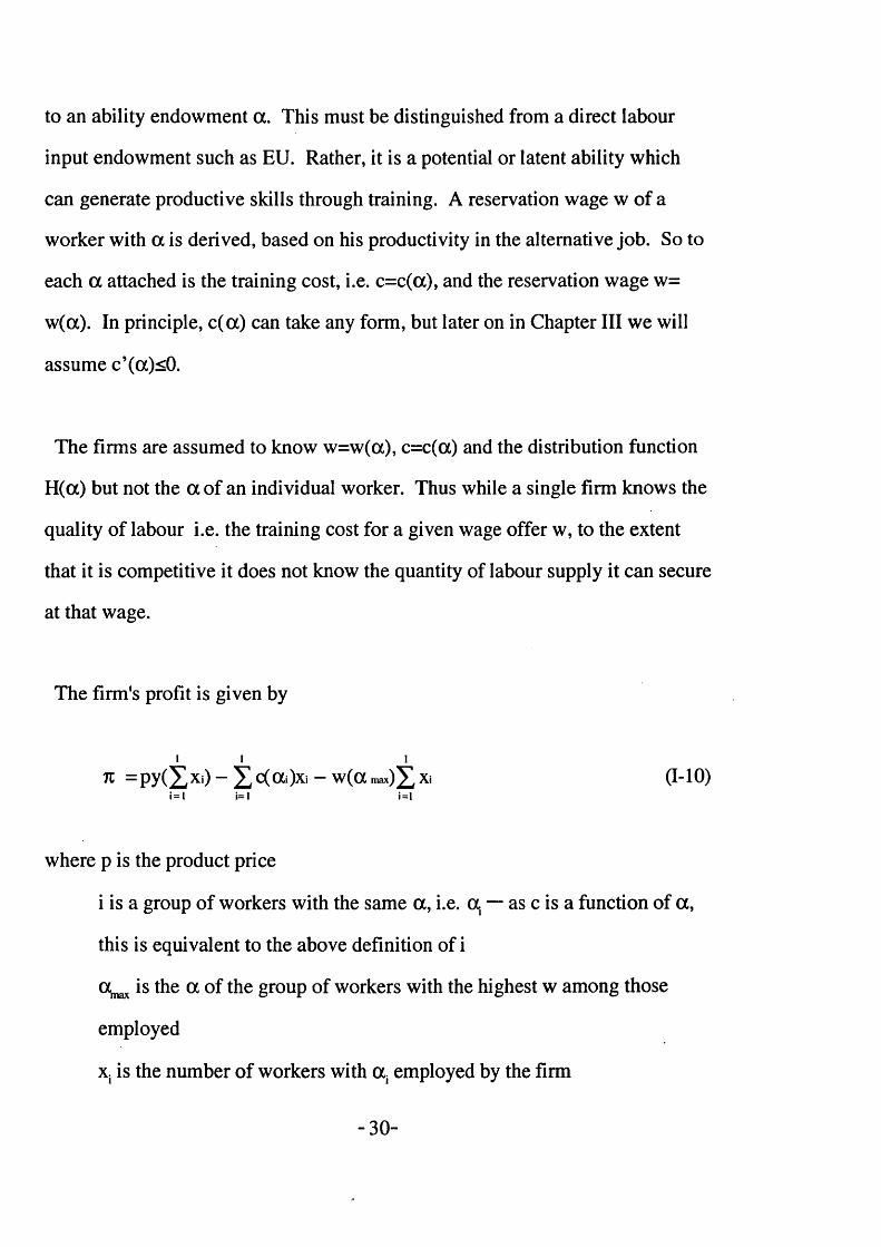
to an ability endowment a . This must be distinguished from a direct labour
input endowment such as EU. Rather, it is a potential or latent ability which
can generate productive skills through training. A reservation wage w of a
worker with a is derived, based on his productivity in the alternative job. So to
each a attached is the training cost, i.e. c=c(a), and the reservation wage w=
w(a). In principle, c(a) can take any form, but later on in Chapter III we will
assume c’(oc)<0.
The firms are assumed to know w=w(a), c=c(a) and the distribution function
H(a) but not the a of an individual worker. Thus while a single firm knows the
quality of labour i.e. the training cost for a given wage offer w, to the extent
that it is competitive it does not know the quantity of labour supply it can secure
at that wage.
The firm's profit is given by
i i i
rc =py ( £ Xi) _ X ° ( a 0Xi - w(ama*)XXi (I-10)i = l i = l i = l
where p is the product price
i is a group of workers with the same a , i.e. a, — as c is a function of a ,
this is equivalent to the above definition of i
ocmax *s a ° f group of workers with the highest w among those
employed
Xj is the number of workers with c l . employed by the firm
-30-

In continuous form
7c=py(x)-c(a)x-w(a)x (I-H)
where x is now the total labour input
w(a) is the reservation wage of the workers with a — the workers of the
highest ability, which is equivalent to in (1-10)
endowment range between 0 and a
The firm is, then, to maximize n with respect to a and x. The formal analysis
will be given in Chapter III and thus I only point out here that the firm quotes
the wage offer and the number of workers it wishes to employ — so it is not a
price taker in the perfect competition sense, but whether this demand is met
depends on the supply condition — so it acts as a competitive firm.
Thus what we attempt to introduce here is a model of heterogeneous labour
market with training. Its basic premises are that a labour market is essentially a
training market, to which workers without skills enter to receive training and
then work, and that the workers are heterogeneous in some innate ability, which
generates the heterogeneity in the training cost as well as in the reservation
Jc(z)dH(z)i.e. the average training cost of the workers with the
-31-

wage. A competitive firm needs to offer a wage to minimize the labour cost
which consists of wage cost and training cost.
This model differs from the Thurow’s job competition model and the Weiss’s
adverse selection model in several ways. As pointed out earlier on, our model
follows the concept of a labour market as a training market employed by
Thurow (1975). But it is more theoretically rigorous than the Thurow’s model.
In particular, the wage is endogeneously determined within the theoretical
framework rather than exogeneously given.
As with Weiss (1980), its limitations discussed in the earlier part of this
chapter are cleared by using an innate ability a rather than the efficiency unit 0.
This is brought about by the use of a function c(a) instead of q(w). For exam
ple, it was explained that as w(0) is assumed to be monotonically increasing if a
worker is more productive in the present firm i.e. high 0, he is also more produc
tive in the alternative sector i.e. high w, but this does not always have to hold.
For our model, c(a) is not required to be a monotonic function so that we do not
have to limit our analysis to the “all-round productive ability” cases. For our
model the adverse selection implies an increase in wage to cause a decrease in
c(a), i.e. c ‘(oc)<0. But there is no guarantee that the total labour cost will be
reduced or equivalently, that the “efficiency wage” always exists. While for the
Weiss model the existence of the efficiency wage was not questioned for the
reason given in the earlier part of this chapter. Finally, we would like to know
how the market characteristics determine the level of efficiency wage. While
-32-

Weiss (1980) offers no suggestion on this issue — the efficiency wage is invari
ant across all jobs, we attempt to relate the training aspect of a labour market to
the wage levels as well as to the characteristics of the market equilibrium.
In this chapter we have discussed the following:
Firstly, the efficiency wage hypothesis (EWH) and the four types of labour
market models based on this hypothesis, namely, the nutritional model, the
shirking model, the adverse selection model and the sociological model, were
introduced and their mechanisms were briefly described. With the adverse
selection effect or the incentive effect as the key concept, these models help to
explain the existence of wage rigidity and involuntary unemployment.
Secondly, the model by Weiss (1980) was examined in detail. Theoretical
difficulties and limitations of the efficiency wage models were discussed. One
such difficulty is that the involuntary unemployment may be eliminated by an
alternative contract characterized by a performance bond, an employment fee or
a piece rate payment or a self-selection or screening device, though this could
be counterargued. It was also shown that the fundamental assumption of ef
ficiency unit restricts the operation of the efficiency wage models in several
ways. First, it restricts the workers to be all-round productive. Second, the
adverse selection is treated as if it is the sufficient condition for the existence of
an efficiency wage. And thirdly, no analysis is given to explain when the
excess supply of labour is likely to occur.
-33-
Thirdly, a job competition model by Thurow (1975) was introduced and its
mechanism, in which training plays an important role, was described. And
finally, a training model based on the concept of Thurow (1975) as well as that
of the efficiency wage was introduced.
The remaining chapters are organized as follows:
Chapter II offers a selected survey of the literature on theories of wage determi
nation and a more detailed survey on training models. It is intended to give
readers some comparative perspectives of this issue and in particular the reasons
why the training model is offered in this work. In Chapter III the model is
presented formally and the labour market equilibrium is established Chapter IV
gives some space to the explanation of why the uniform wage may be assumed;
or, in other words, to examine the conditions in which the equilibrium so estab
lished in the previous chapter is robust. Chapter V offers a two-period model of
training with heterogeneous labour, in which an upward-sloping wage profile is
derived. Chapter VI looks at this competitive equilibrium of the heterogeneous
labour market in comparison with monopsony equilibrium, using the
Lagrangian multiplier method. Comparative static analysis appears in Chapter
VII, in which several policy implications are discussed. Chapters VIII and IX
look at slightly different models of labour market by modifying some of the
assumptions of the original model — Chapter VIII looks at a case of heter
ogeneous firms as well as workers, which is then followed in Chapter IX by a
- 3 4 -

case of observationally distinguishable workers. In both cases, the equilibrium
is established and the comparative static analysis is offered in an analogous
manner to that of the original model. Each chapter ends with a brief summary
of the results established in that chapter. And finally the conclusion appears in
Chapter X.

CHAPTER I I : A SURVEY OF LITERATURE ON THEORIES OF WAGE
DETERMINATION
In this chapter we survey the literature on wage determination theories. The
theories are presented in a basically chronological manner to illustrate a brief
history of the theories of wage determination mechanism. There is a wide
variety of approaches offering explanations of wage determination mechanism.
And this chapter intends to contrast them and offer comparative perspectives to
this issue.
The chapter proceeds as follows. Firstly the overall view is presented to
describe how the issue of wage determination has been tackled in the past.
Secondly the theories are grouped into 'approaches' in terms of assumptions and
basic framework of models. Here the focus of each approach is clarified and its
merits and demerits in employing as a model to describe the labour market
mechanism are assessed in turn. Then we have a closer look at theoretical and
empirical works on economics of training. Finally, these are contrasted with the
approach followed in this work.
(1) The Overall View
One way to systematically survey the literature on the theories of wage determi
nation is to categorize them into the following three groups; (a) a determination
-36-

of wage level, (b) a determination of wage differentials, and (c) a determination
of wage distribution. Each group pursues the analysis of the labour market
from a slightly different angle from the others. The orthodox neo-classical
income distribution approach falls into (a), the first group. The approach pre
sents a labour market within an overall picture of economy in terms of general
equilibrium analysis. It shows how the wage level is determined in relation to
other prices. However, when one wishes to investigate the reason for the exist
ence of wage differentials i.e. ( b ) , the second group, one needs a more detailed
analysis within one labour market. Thus the human capital approach serves to
explain how and why an individual with particular characteristics earns a wage
different from others. The institutional approach also shows how persons with
different attributes obtain employment in different sectors, thus generating a
structure of wage differentials. As for the question of the shape of a wage
distribution i.e. (c), the third group, some have been puzzled by its lognormal
shape. The statistical/mathematical approach was presented in 1950’s, which
was then followed by the more economically meaningful job matching ap
proach.
All these approaches assume perfect information. However, with a growing
interest in the economics of information since Stigler (1961) through Akerlof
(1970), there has been a line of approaches in the field of wage determination
parallel to those presented above but with an assumption of imperfect informa
tion. Thus the implicit contract approach attempts to explain how a wage is
determined — i.e. (a) — when the level of output is not known with certainty in
-37-
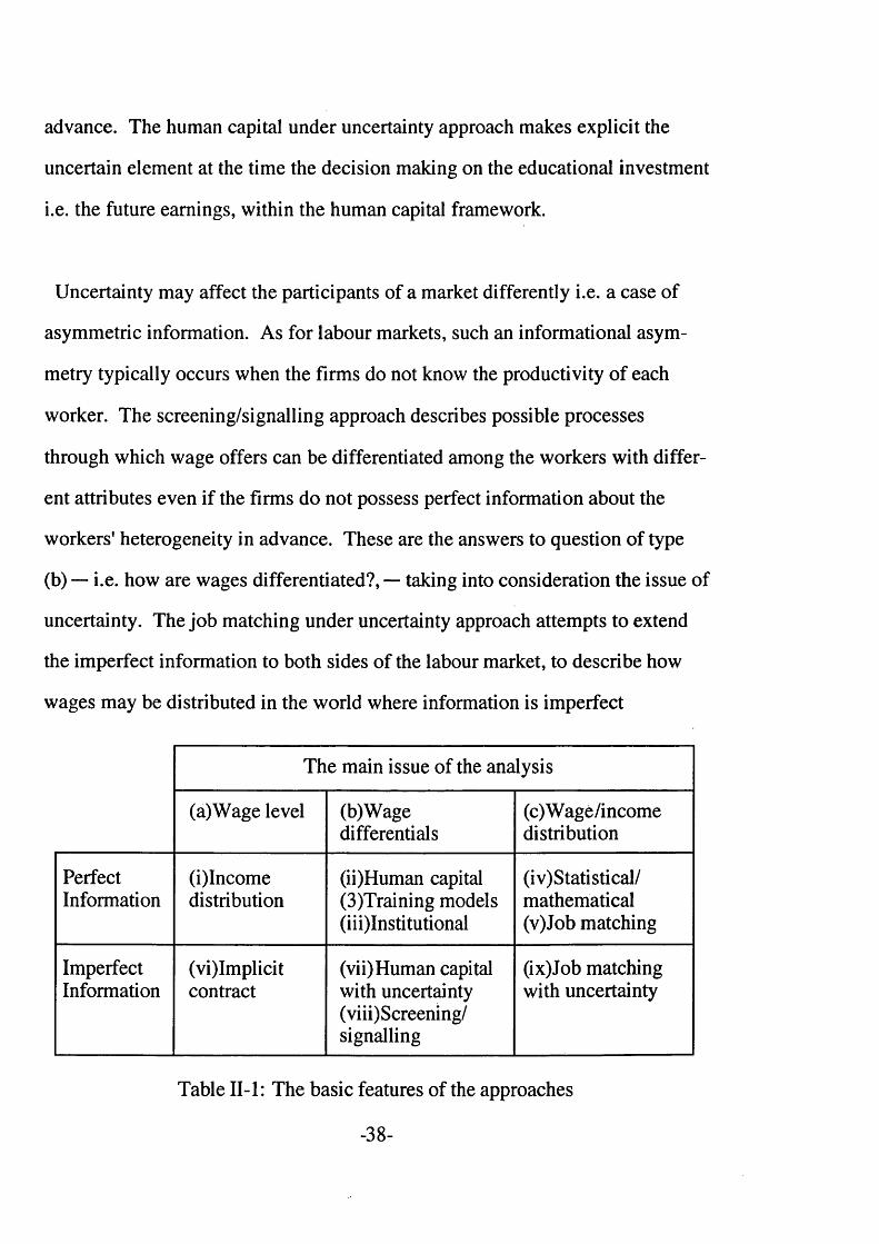
advance. The human capital under uncertainty approach makes explicit the
uncertain element at the time the decision making on the educational investment
i.e. the future earnings, within the human capital framework.
Uncertainty may affect the participants of a market differently i.e. a case of
asymmetric information. As for labour markets, such an informational asym
metry typically occurs when the firms do not know the productivity of each
worker. The screening/signalling approach describes possible processes
through which wage offers can be differentiated among the workers with differ
ent attributes even if the firms do not possess perfect information about the
workers' heterogeneity in advance. These are the answers to question of type
(b) —■ i.e. how are wages differentiated?, — taking into consideration the issue of
uncertainty. The job matching under uncertainty approach attempts to extend
the imperfect information to both sides of the labour market, to describe how
wages may be distributed in the world where information is imperfect
The main issue of the analysis
(a)Wage level (b)Wagedifferentials
(c)Wage/incomedistribution
PerfectInformation
(i)Incomedistribution
(ii)Human capital (3)Training models(iii)Institutional
(iv)Statistical/ mathematical(v)Job matching
ImperfectInformation
(vi)Implicitcontract
(vii)Human capital with uncertainty(viii)Screening/ signalling
(ix)Job matching with uncertainty
Table II-1: The basic features of the approaches
-38-

i.e. the question of type (c). Table II-l illustrates the grouping discussed above
and each approach is explained in the next section in turn..
(2) The Theories
(A) Perfect Information
(i) The Neo-classical Income Distribution Approach
Within a general equilibrium framework, labour demand exists as a derived
demand alongside demand for capital for the production of goods. The wage is
a remuneration for labour service, being determined simultaneously with inter
est as a payment for capital. The firm's profit maximization implies that the
marginal productivity of the each factor is equated to the corresponding remu
neration. The equilibrium wage is determined by the interaction of supply of
and demand for labour as well as that of supply of and demand for capital.
In general, a traded commodity in any one market is assumed to be homoge
neous within this framework. And it is this homogeneity assumption that limits
this type of approach to construct a comprehensive model of a labour market, to
describe a process of wage determination for the following reason. The assump
tion of homogeneity of labour allows only a single wage in the labour market.
Thus, if we wish to describe a labour market in the real world, in which there
are more than one wage, we would need to assume that there is a complete set
of markets for several different types of labour — for example, a skilled labour
-39-
market and an unskilled labour market. In turn, their wages are determined by
the corresponding supply and demand conditions. And while theoretically this
does not restrict the range of wage level in any market, we see in reality that a
wage in some market is most of the time, if not always, higher than in other
market, such as a case of a skilled labour market and an unskilled labour mar
ket. One may argue that a wage of skilled labour tends to be higher than that of
unskilled labour because there is always a shortage of skilled labour relative to
unskilled labour. But then we must answer the next question as to why such a
difference in labour supply exists. It would be necessary to say something
about the way by which one decides to supply his labour service to one market
rather than another. Within the general equilibrium framework, such an exten
sion could make the analysis too complicated to produce some simple and clear
results.
Therefore, while this approach ought to be credited for its focus on the analysis
of an overall picture of an economy and hence the analysis of a labour market in
relation to other markets in the economy, it cannot go very far in explaining the
pronounced phenomena in labour markets such as the existence of wage dif
ferentials.
(ii) The Human Capital Approach
The labour earnings of a worker may be found to be correlated with his at
tributes such as years of schooling, sex, race or the amount of working experi
ence. Human capital theorists argue that education is an investment that gener
-40-
ates higher earnings as a return in the future, so that the educational decision is
analogous to investment decisions of capital. (See, for example, Shultz (1965),
Mincer (1974), Becker (1975)) They maintain also that such an investment
extends into one’s working life in the form of 'On-the-Job Training (OJT)\ This
training aspect is dealt with in the nest section in detail.
This approach has three main contributions to the understanding of labour
market operations. Firstly, by treating an educational decision as an economic
issue, it has questioned the orthodox educational philosophy and the one that
many people hold namely that the value of education cannot be rightly mea
sured in monetary terms alone. Secondly, the OJT hypothesis gives an explana
tion to an upward-sloping shape of a typical age-earning profile. And thirdly it
is important to point out that many empirical works have been done based on
the human capital theory, using an "earnings equation" of the form : lnYs=
lnY0+rs, where s is years of education, Y. is the earnings of a person with i years
of education, and r is a rate of return. I would like to emphasize it here because
many theories in this field of labour economics are interesting but difficult to
test empirically.
As for our immediate concern, this approach can deal with the issue of how
wages are determined and differentiated in terms of the level of investment in
education and OJT. By giving some insight into decision making on education
and/or OJT, it attempts to rationalize observed wage differentials in terms of an
optimization process. It thus solves the problem faced in the neo-classical
4 1 -

income distribution approach as a result of having to set up one labour market
for each wage to be determined. In fact, the human capital theory is a labour
supply analysis, since it describes how a potential supplier of labour determines
the amount of investment in himself by examining how much earnings can be
generated in the future. However, as an educational investment requires some
time to generate its return, the future earnings is likely to bear a considerable
degree of uncertainty in two ways — namely, uncertainty about the successful
educational achievement and uncertainty about the condition of the demand for
the type of labour. The approach could reflect the reality more by taking these
uncertainties into the model (See (vii)).
(iii) The Institutional Approach
The models in this group all have quite intuitively appealing features, as their
structures are based on historical, institutional or qualitative aspects of labour
markets. At the same time, however, their assumptions in some cases do appear
to be rather ad hoc to Neo-classical economists. In fact the works we refer to in
this category follow the line of what is often called the segmented labour market
theories. Their starting point is the questioning of the neo-classical theory of
labour markets. For example, they point out that the persistence of poverty and
income inequality despite the long-standing policies to eliminate them can not
be explained by the neo-classical theory. Cain (1976) offers an extensive
survey on the segmented labour market theories.
Two of the more notable works on these theories are the dual labour market
-42-

theory of Doeringer & Piore (1971) and the job competition theory of Thurow
(1975). The dual labour market consists of a primary labour market offering a
job with a higher wage, better working conditions, more promotion possibilities
and more stable work, and a secondary market offering the opposite of what the
primary market is offering. While workers in the primary market have no
intention to leave for the secondary market, workers in the secondary market
become accustomed to the working patterns of that sector and find it difficult to
move out of this inferior sector of the society and thus these two types of labour
markets continue to coexist. With the job competition theory, there are two
types of market mechanisms called Job Competition and Wage Competition.
Under job competition numbers and types of job slots are technologically
determined. Wages are not principally determined by market forces. In fact
there said to be a persistent job queue, from which firms choose the better
workers. Consequently firms use some screening device to select better work
ers. In contrast, wage competition is what is normally known as a neo-classical
market-clearing case. By pointing out that workers of different abilities may
receive the same wage under the job competition, Thurow suggests that a wage
is paid according to productivity required for the job rather than productivity of
the worker. As a consequence, workers are recruited to receive OJT to be able
to perform the required jobs.
The main difficulty with these theories is that their presentations are rather
descriptive. For example, in the dual labour market analysis it does not explain
how one market comes to be considered as a secondary rather than a primary
4 3 -

market. Or there is no clear explanation in the job competition theory as to how
the wage was determined in the first place. Because of this, as Cain (1976)
points out, their criticisms of the neo-classical theory are not substantial.
Bhagwati (1977) and Fields (1974) both attempt to model a theory of ed
ucation in LDC economy, in which the supply of and demand for the educated
workers do not always match. In particular, they describe as 'Job Ladder and
Faimess-in-hiring1 and 'Bumping' respectively a phenomenon of hiring the
better workers first when there is an excess supply of workers. The focus of
these works is, however, on the social efficiency/inefficiency of education
rather than how the wages are determined and as a result they do not offer a
convincing mechanism of wage determination. Similarly the system of labour
market, i.e. the job ladder model, the flexible wage model, or the social opti
mum model for Bhagwati (1977) or the bumping model, the stratification mod
el, or the pooling model for Fields (1974) is a 'choice variable'. Thus, for exam
ple, Fields (1974) does recommend one system as the socially most efficient
one but can not guarantee that the efficient system prevails as a stable or robust
equilibrium.
(iv) The Statistical/Mathematical Approach
At the end of the last century, Pareto (1897) observed that the distribution of
income was not symmetric around its mean but rather it is skewed to the right.
He derived what is now known as a Pareto distribution to fit this right-skewed
income distribution data. It was realized later, however, that this theoretical
-44-

distribution does not fit well the lower end of the actual income distribution.
Gibrat (1931) presented a lognormal distribution as an improved version of the
Pareto model, to fit well the lower end of the actual income distribution. Var
ious attempts to explain this skewness of the distribution to this day include
Champemowne (1953) and Roy (1950).
Champernowne (1953) employed a theory of stochastic process of the Markov
chain type. Given continuous flows of income, he assumed that a probability of
falling into a certain income group as a result of an annual change of income
follows a certain pattern. He concluded that in a steady state the distribution of
income becomes Pareto or lognormal irrespective of the initial state of the
distribution. In other words, the Pareto or lognormal shape of the income
distribution is the result of continuous income changes that occur following
some probabilistic laws. This theory seems to offer a very simple and yet
appealing explanation to the observed skewness of the income distribution. His
argument relies heavily on his two basic assumptions. Firstly, the presently
observed distribution is assumed to be in the steady state. However, as Lydall
(1968) pointed out, one's life may not be sufficiently long to generate the steady
state and thus his income is more likely to be conditional upon his initial endow
ment at the beginning of his life. Secondly, the annual income change is as
sumed to follow a certain pattern of stochastic process. However, no economic
interpretation is given in the specification of this process. Although one needs
not deny the stochastic factor in the income generating mechanism, it is hard to
believe that such a mechanism operates independently of economic factors.

Thus the theory would have been more convincing if its stochastic process had
been constructed explicitly on the concept of economic rationality.
Others attributed the cause of income differentials to the ability distribution.
To them, however, the crucial issue was to explain what is called the Pigou
paradox, that is, a paradox that despite the normally distributed ability the
distribution of its derivative i.e. income, is not. (See, for example, Pigou (1932))
Roy (1950) suggested that ability has several dimensions such as intelligence,
physical strength, decisiveness and leadership, and showed that when these
normally distributed dimensions are multiplicatively combined it produces a
lognormal distribution of income. The criticism of this approach is two-fold.
Firstly, what we define here as ability are difficult to quantify and consequently
it is difficult to actually prove that they are all normally distributed, let alone the
determination of its multiplicative distribution. Secondly, it faces the same
criticism as that of the Pareto model and the Champemowne model, in that it
does not take into consideration the complex interaction of market forces.
(v) The Job Matching Approach
The models of this approach assume heterogeneities of both workers and jobs
within a single market. Tinbergen (1951) & (1956) and Lucas (1977) consider
continuous heterogeneity in both workers ability and job type. The equilibrium
then entails a wage equation, a continuous functional relationship between wage
and job/worker attribute. (See Tinbergen (1951) & (1956)) And the wage per
unit of attribute is often called a Hedonic Wage. (See Lucas (1977)) The idea of
-46-
attaching some monetary value to each attribute of a traded commodity is the
concept of Hedonic Price and a more general model of this type is found in
Rosen (1974). Such a concept is useful for analyzing a market for commodities
of a high degree of heterogeneity such as houses or cars as well as labour ser
vice. For purchasing a house, for example, one takes into consideration many
of its attributes as well as the price itself such as a condition of the house, its
size and of its garden, a number of rooms, and its geographical characteristics
e.g. its distance to the workplace, or natural and social environment. And the
hedonic price of an attribute is the market value attached to a unit of each
attribute.
Tinbergen (1956) considered the matching of a demand distribution for labour
and a supply distribution of labour. A job in the demand distribution or a
worker in the supply distribution is characterized by several attributes by means
of its degree. Thus, for example, a worker may possess a high degree of intel
ligence and yet a low degree of ability to deal with others, or a job may be
described by a low degree of precision and a high degree of cooperation among
fellow workers. The degrees are measured on a continuous scale of each at
tribute. His argument is that because these two multivariate distributions on the
continuous scale are not necessarily identical, there is a need for what he calls
an income scale to match these distributions, through which the income distribu
tion may be determined. Assuming that the supply and demand distributions to
be bivariate normal distributions and that the supply is wage elastic and the
demand is not, he solves the problem as a workers’ utility maximization to
-47-
obtain the income scale, with the additional condition that supply and demand
for each job are equated. He then attempts to generalize the result for the case
where the demand distribution is also wage elastic. However, he points out that
such a generalization would be possible but extremely complicated and does not
present a general solution.
As for the hedonic theories, their contributions to empirical studies have been
considerable as the concept of hedonic price/wage is appealing. The human
capital model may fall under this category as far as its empirical aspect is con
cerned. At the theoretical level, attempts have been concentrated on investigat
ing whether the standard results of general equilibrium analysis are valid in the
hedonic or implicit market cases. What appears to be missed out in this ap
proach, however, is the issue of imperfect information about the heterogeneities
of firms and workers. The equilibrium wage in this model of labour market
corresponds to a set of continuous values of wages known as a wage equation.
And to each wage level on this wage equation there is a pair of a firm and a
worker at the equilibrium. With the full information every agent in the labour
market may be able to find his best partner. However, it would be difficult to
see that this result holds when the information is less than perfect. And this is
the issue we turn to in the next section.
(B) Imperfect Information
(vi) The Implicit Contract Approach
The original idea of the implicit contract was due to Baily (1974), Gordon
4 8 -
(1974) and Azariadis (1975) in the mid 70’s. The approach attempted to find an
answer to the real world observations that the competitive labour market anal
ysis could not explain the — namely, the wage rigidity and an existence of
involuntary unemployment. Consider a risk-neutral firm and homogeneous
risk-averse workers in a situation of uncertain demand for products. Acting also
as an insurer, the employer is more likely to offer a labour contract with a
somewhat lower but fixed wage irrespective of the state of world that would
actually occur. However, the models do not always generate involuntary unem
ployment.
More recently, asymmetric information is introduced into the analysis, while
the earlier models assumed symmetric information about the state of world as
both firm and workers can observe it. Hence, a firm and workers do not have
the same degree of access to information on, for example, the state of world
the firms are more informed (See Grossman & Hart (1983)), or the reservation
wages — the workers are more informed (See Moore (1985)). For surveys, see
Rosen (1985) and Manning (1990).
There is no doubt that the approach has given a further insight into understand
ing of the wage determination by taking into account the aspect of uncertainty.
However, to the extent that most of results here do not depend on the assump
tion of heterogeneous labour, it is not quite the ideal approach for understanding
the reason for the observed wide variety of wage levels in reality.
-49-

(vii) The Human Capital under Uncertainty Approach
In its simplest form human capital models do not usually assume that risks are
involved in the investment. It goes without saying, however, that the risk
element is the important factor in anyone's educational decision making. There
are two types of risks in human capital investment. One is the risk involved in
how well the investment programme goes. And the other is how well the prod
uct i.e. labour after human capital investment, will be valued in the labour
market.
Levhari & Weiss (1974) define the two types of risk or uncertainty — input
uncertainty and output uncertainty. The former is due to uncertainty about one's
own ability to follow the education or about the quality of the education. The
latter refers to uncertainty about future supply and demand conditions in the
labour market. Their theoretical work concludes among other things that; (i) the
optimal level of educational investment is higher for a higher level of inherited
wealth, (ii) the increase in the degree of uncertainty reduces the investment, but
(iii) the effect of the level of interest rate on the investment level is ambiguous
in fact this depends on whether the investor is a net borrower or net lender.
One of the empirical works on the human capital investment with uncertainty is
given in 01 son,White & Shefrin (1979). They examine the degree of income
variation in relation to the attributes of workers such as years of schooling. For
those potential students, a large income variation in the future given a certain
level of education means a high degree of uncertainty for receiving that level of
education. They conclude, 'Our empirical results indicate that college should be
-50-

taken as a package or not at all, due to the large positive effect of the fourth year
of college', as income variation for those with less than four full years of college
education is found to be larger than those with the full four years.
This approach is much more realistic than the human capital approach de
scribed earlier, as the risks in human capital investment are taken into consider
ation. However, the approach does not go beyond the analysis of labour supply.
As for our principal interest lies in the wage determination mechanism and in
particular the wage differential mechanism, we need to look more into the
interaction of supply and demand.
(viii) The Screening/Signalling Approach
Educational achievement may be used by firms to "screen" the heterogeneous
labour force, when the firms do not have information about productivity of each
individual worker. With an assumption that a worker with higher productivity
does better in education also, a higher educational achievement implies a higher
wage. Contrast this with the human capital theory — educational achievement
as a screening device merely raises one's earnings relative to others' without
raising productivity, while if it is human capital investment it would raise the
earnings through an increase in productivity. (Note here that they both imply a
positive relationship between educational achievement and earnings.) Stiglitz
(1975) shows that there may be multiple equilibria and an equilibrium with
screening may be Pareto inferior to others, implying that such an equilibrium
may not be socially desirable.
-51-

Signalling is another term often used when a market is characterized by infor
mational asymmetry. The distinction between signalling and screening is not
exactly an established concept. To some it is the order of move that matters — it
is screening if the uninformed player moves first and signalling if the informed
player moves first. (See Rasmusen (1989), Stiglitz & Weiss (1994)). To others
such as Kreps (1990) the situation is defined as screening if the uninformed side
proposes a menu of contracts among which the informed side selects, while it
would be signalling if informed side takes the active role. Here we avoid the
discussion to be too technical and merely mention that in a labour market the
workers i.e. the informed players, obtain education to signal, while the firms i.e.
the uninformed players, use the education to screen. Signalling may be also
used in a more general sense to describe the informational equilibrium, since the
introduction of the term by Spence (1973).
A firm may attempt to acquire information on worker's productive ability
using a "self-selection" device upon their application. A self-selection device is
a scheme that causes the worker to reveal truthful information about oneself.
Such a device may be an application fee (See Guasch & Weiss (1981)), a wage
schedule contingent upon a test result (See Guasch & Weiss (1980)), or the both
and a test with a cutoff level (See Guasch & Weiss (1982)). One of the earlier
discussions on the self-selection mechanism was presented by Rothschild &
Stiglitz (1976). They modelled the imperfect information in an insurance
market. An insurance firm offers a set of contracts to heterogeneous customers.
-52-
The equilibrium may be characterized as a pooling equilibrium in which custom
ers all buy the same contract or as a separating equilibrium in which different
customers buy different contracts or there may not be an equilibrium at all.
This idea is also used in the field of labour economics when, for example, the
firm does not know the productive ability of each worker drawn form a heter
ogeneous labour force. A pooling equilibrium would be the equilibrium in
which all the workers are paid the uniform wage, while a separating equilibrium
is characterized by wage differentials based on the heterogeneity of the workers.
(See Chapter IV, in which the argument is employed to derive a condition for
the uniform wage system of payment.)
This approach explicitly analyses the consequences of imperfect information,
while such was not explicitly taken into consideration with the model of a
heterogeneous labour market described earlier in this chapter such as those of
the job matching approach. It is also worth mentioning that this approach
explicitly examines the robustness of an equilibrium. My objection to this
approach are two-fold. Firstly, the analysis has become quite technical as more
emphasis is placed on the nature of equilibrium. And it is doubtful that the
suggested set of contracts is actually implementable in the real world — in
reality such detailed and explicitly stated contracts are quite rare. That is proba
bly because such a system of employment contract can be extremely complex
and thus costly and time consuming to create and implement in the real world of
high degree of worker's heterogeneity. Secondly, firms might be more interest
ed in devoting time for training the workers to perform the job rather than for
-53-

selecting the optimal workers. This is consistent with the basic concept of OJT,
as described in Thurow (1975).
(ix) The Job Matching under Uncertainty Approach
Here heterogeneity is assumed on the both sides of the market. The firms do
not possess information on the productivity of each worker as in the models
discussed earlier on in this chapter. What makes this approach different is the
assumption that the workers' productivity depends on the job, or, to put it differ
ently, there are better matching and worse matching of workers and firms. The
main result is that as long as there are no workers who have an absolute advan
tage in all jobs, accurate information is beneficial. (See MacDonald (1980))
Jovanovic (1979) relates job matching and turnover in such a way that higher
productivity generating job matching tends to give a lower turnover rate. With
this approach, the emphasis lies on seeking the most efficient matching possible
within this framework. Consequently, as the production function takes the
simplest form, how wages are determined is not the main issue in this approach.
The main difficulty with job matching models in general lies in the treatment
of heterogeneities. The more sophisticated we assume the heterogeneity to be,
the more complicated the operation of the model will be. If the uncertainty is
further assumed, its analysis would be extremely complicated.
(3) Training Models of a Labour Market
-54-

So far we have been assuming the labour market as a market for trained labour
so that the newly recruited workers can fully participate in the production right
away. However, many dispute this proposition and argue that labour needs
further adjustment to perform the required job. They maintain that training of a
worker exits as a process of human capital formation which continues through
out one’s working life and put much more emphasis on the nature of training
than on the supply and demand interaction of the labour market. This section is
intended to introduce the basic concepts as well as theoretical models and
empirical evidence of training.
Training is an investment in human capital in the same way as education is.
Thus, the more training one receives the more productive he will be. The
obvious difference between the two is that training is usually given after the
labour contract is agreed while education takes place before the employment.
More importantly, training is more purpose-specific in a sense that a worker
usually receives training with some specific job in mind while education tends
to serve for a more general purpose. Training may be categorized into “off-the-
job”, which is given to workers when they are not engaged in production, and
“on-the-job”, which is said to take place alongside the production. Much empha
sis is given to this latter type of training for at least two reasons. Firstly, many
labour economists, for example Becker (1964), believe that the best training is
“leaming-by-doing,” or “leaming-through-experience,” in a sense that although
theories may be taught at school, practice is best acquired at the workplace.
Secondly, this idea of leaming-by-doing helps to explains the observed upward-
-55-
sloping wage profile — one’s wage rises by experience because productivity
increases through this learning-by-doing.
On of the early works on the economic analysis of training was Becker (1964).
He argued that there are two types of OJT; general and specific. General train
ing increases the productivity of the trainee at the training firm and at any other
firm to exactly the same extent, while specific training does not raise the train
ee’s productivity except in the training firm. Becker (1964) illustrated his
argument by referring to various types of training given to military officers in
the U.S. At one end of the spectrum learning how to fly an aircraft is fully
general training since the skill can be used in the civilian sector. The author
referred to the fact that “well over 90% of the U.S. commercial airline pilots
received much of their training in the armed force.” On the other hand, if one is
trained to be an astronaut, a fighter pilot or a missile man, there is not much that
he can do to increase his productivity in the civilian sector and this would be a
fully specific training. In general, however, the most types of training have both
aspects. He then argued that the cost of general training is bom by the trainee,
since it is an investment that the training firm can not secure its return. His
argument for the cost of specific training is that it would be shared by both
parties as they both try to take a precautionary step to a possible turnover — the
firm would fail to capture the return if the worker quits and the worker fails to
capture the return if he is fired.
A more explicit argument on the incidence of specific training cost is found in
-56-

the transactions cost model of Hashimoto (1981). When there exist some values
that the both the firm and the worker can not agree costlessly, such as the value
of the marginal product of the worker in the training firm or in the alternative
firm, a positive transactions cost is said to exist. This in turn could cause the
separation of the worker and the firm, even if this means making the both worse
off. And in such a case the cost of as well as the return to the specific training
are likely to be shared. Katz & Ziderman (1990) questioned the Beckerian
preposition on the incidence of general training cost. Their argument is that due
to an informational asymmetry between a training firm and a recruiting firm
about the extent and the type of the training the latter does not value the worker
as high as the former and this discourages the trainee to pay for the general
training. The interesting point in their argument is that the distinction between
general and specific training lies greatly on the informational asymmetry rather
than the actual nature of the training.
Stevens (1994) also reconsidered the Beckerian classification of general vs.
specific OJT, of which most types of training are said to be combinations of the
two with differing degrees. Her argument is that while specific training is
useful to the training firm alone, which corresponds to pure monopsony, and
general training is useful to all the firms, which corresponds to perfect competi
tion, other types of training are useful to some firms, which corresponds to the
imperfect competition. In this last case, the training is defined as “transferable”
and the firm may finance it, as they hold monopsonic power to capture the
return to the training. And this explains the observation that firms pay for
-57-

training even if it does not appear to be specific — it is then transferable rather
than general. Stevens( 1994c) points out that there could be two types of inef
ficiency when a firm provides training to workers. As in Stevens( 1994b), she
defines training as transferable and argues that the imperfect competition among
the firms in the labour market causes inefficiency while the information asym
metry concerning the value of the trained worker also causes an allocation
inefficiency. With a simple example of two firms and one worker, she suggests
that the inefficiency may be reduced if the participants of the market follow a
labour contract in which firms set a wage offer after the training is completed as
opposed to contracts with a predetermined wage or in which a worker sets the
wage.
Specificity of training is also questioned by Acemoglu (1997). He argues that
a large portion of the investment in training in Japan and Germany, where the
level of training is high, is general rather than firm-specific and yet it is fi
nanced by the training firm rather than by the workers. In his model, workers
and firms have costly search to find a partner, or the labour market is said to be
‘frictional’ as opposed to a frictionless competitive market. Then some of the
return to training is captured by the future employer firm rather than by the
training firm or the worker and this causes underinvestment of the training. As
for the reason why the training firm pays for the general training, he explains
that this costly search allows the training firm to capture some of the return to
the training and thus it does not lose by financing the general training. Put it
differently, the general training becomes specific to the extent that the workers
-58-
can not costly change the employer because of the friction. He further argues
that the workers would invest in their skills and accept to receive a low wage
today to receive a higher wage tomorrow if the firms are more willing to in
novate, since innovations raises their return to training. Turnover also is ex
plained within the framework of general training rather than specific training in
his model.
A few training models have also been developed by those who consider that
labour markets are essentially markets for training. The job competition model
of Thurow (1976) was mentioned in Chapter I as one of these approaches.
Ishikawa (1981) constructed a model of dual labour market, in which he offered
a generalization of Thurow’s job competition. He pointed out that the “ed
ucational paradox” of the 60’s and 70’s U.S., the occurrence that education
functioned neither as human capital nor screening — a general increase in the
educational level of the nation did not affect the size distribution of income
significantly, can be explained by characterizing the U.S. labour market as a job
competition model. Here the emphasis of the analysis is on the macroeconomic
dynamics of the labour market rather than how a particular training scheme
affect the equilibrium of a labour market. Bosworth, Wilson & Assefa (1993)
argued that the employment relationship between a worker and a firm is a
dynamic relationship through which continuous investment on labour is made in
the form of training. Thus we may talk of a “market for training” rather than a
market for trained labour, in which the extent and nature of the training activity
to be given to workers are determined from the demand for and supply of

trained individuals. They offer the general direction in the labour market anal
ysis — a dynamic model of a market for training is necessary to understand
training investment behaviour, but fail to offer a specific model.
A more rigorous and theoretical model is found in Felli & Harris(1996), who
introduces a dynamic model of training behaviour with specific training generat
ing an upward-sloping wage profile. Every wage along the equilibrium wage
profile consists of three components — the opportunity wage, a premium reflect
ing what the worker would have accumulated if he was in the alternative job,
and a reduction reflecting what the worker would have lost if he was in the
alternative job. It is shown that along the time path the wage rises, implying
that there are positive returns to tenure i.e. the wage profile is upward-sloping.
The intuition behind this result is that the human capital is interpreted as infor
mation and thus accumulates over time, causing the value of the specific human
capital i.e. wage to rise along the time path.
Salop (1979) offered a unique model of training within the efficiency wage
framework. Although it was introduced in Chapter I as a turnover model, I
mention it again as it is also one of the well-known training model. His workers
are required to be trained at the initial period, while their turnover rate is neg
atively related to the wage offer. Thus the higher wage implies a group of
workers with a generally lower incentive to quit and this means a less number of
new workers to train and so a lower training cost to the training firm. As a
result there exists a wage that maximizes that profit, as opposed to a usual profit
-60-

maximizing problem in which the wage is exogeneously given. Salop (1979)
assumed the training cost is paid by the training firm and there is no explicit
discussion about the incidence as in Becker (1964), Hashimoto (1981), Katz &
Ziderman (1990) or Stevens (1994). The incidence of training cost is discussed
in Salop & Salop (1976) within a basically same framework as in Salop
(1979)’s. But with the cost of training invariant across workers, the detailed
analysis on how the training cost could affect the equilibrium of the labour
market is not given in either of them.
A list of empirical works on the training issue is far more extensive than that
of the theoretical counterpart illustrated above. The type of training varies
between on-the-job and off-the-job, formal and informal, privately given and
publicly given, or general and specific, but the most of these empirical investiga
tions focus on the two issues, the upward-sloping wage profile or positive return
to tenure, and the job mobility or turnover. Recall the Beckerian classification
of general and specific training. If training is general, the worker pays for the
training to acquire higher productivity after the training to earn a wage increase.
As a result, we observe an upward-sloping wage profile. If, on the other hand,
the training is specific, the wage profile can still be upward-sloping but not for
the productivity increase. In this case, such a wage profile is set by the training
firm to keep the trainee after the training, as the trained worker has added
productivity for the training firm while the trained worker has no merit to stay
on. With the specific training, the turnover is said to decrease for the same
reason — the longer the worker stays in the firm the greater his productivity
-61-

contribution will be and thus the firm makes more effort to keep him.
Barron, Black & Loewenstein (1989) examined the U.S. survey on the OJT
activities in 1982 and observed that “on average a new worker spends over 150
hours in OJT during the first three months of employment.” They suggested
with the same data that there is a direct relation between the level of training
and productivity growth and that at least a half of training is specific because
about a half of the returns to training is received by a worker. A word of cau
tion is found in Ashenfelter & Card (1985) for dealing with actual data to esti
mate the effect of training programme on earnings. Using the U.S. data of the
Continuous Longitudinal Manpower Survey, they estimated the wage return to
training of the Comprehensive Employment Act training programme. The
results were in general supportive of the positive effect of training. However, it
was pointed out that those who received the training tended to have a low
income in the period immediately before the programme — in fact, it is not
surprising since the progremme was geared towards those in most need, and
thus had to be corrected against the overestimation .
Clearly, not everyone in the society receives the training, or to the same extent
even if they receive one. The recipients of training are described in Greenhalgh
& Stewart (1987), Altonji & Spletzer (1991), and Booth (1991). In Greenhalgh
& Stewart (1987), the British data of the National Training Survey was used to
show who received training. They found that in general women receive signif
icantly less full-time training than men, and more specifically the higher oc-
-62-
cupational status means more full-time training for men and single women
while for married women the higher status implies more evening training. One
more interesting finding is that the acquired skills depreciates within about a
decade. Data from the National Longitudinal Survey of the High School Class
of 1972 was used in Altonji & Spletzer (1991) to show the link between work
ers’ characteristics and the levels of training. They found, for example, that
women receive less training but happen to pay more than men and that blacks
receive more training than whites. The gender difference in the provision of
training is also pointed out in Booth (1991), who uses the British Social At
titudes Survey of 1987. She finds that the women are less likely to receive
formal training than men of the identical characteristics. Her findings also show
that the levels of general education and training offered are complementary and
that public sector is more likely to offer training than private sector.
Studies in the British apprenticeship were conducted by Booth & Satchell
(1994), Chapman (1993), and Stevens (1994d). Their common concern was the
decline of the number of apprenticeships particularly in the 1980’s. Booth &
Satchell (1994) shows that those with higher educational achievement, with
higher employment status of the father, and who work in large firms, are more
likely to receive apprenticeships. And on the whole the completion of the
apprenticeship makes both workers and firms favour continuing employment
relation. Chapman (1993) offered the evidence of training schemes in the U.K.
For example, in the late 1980’s between a quarter to a third of all 16-18years old
received some training scheme such as the Youth Training Scheme or apprentic-
-63-

es, although an international comparison shows the U.K. has a relatively large
number of workers receiving no training or training of very low quality. He
also suggested that the problem of employers poaching trained workers is cased
by training firms having no property right over the human capital of the trained
workers. And this in turn weakens their incentive to pay for the training and
thus might have been the cause of the insufficient level of training observed in
U.K. Stevens (1994d) searched the reasons for the decline using an investment
model. Skilled labour may be acquired either by training workers or by recruit
ing already skilled workers. She concluded that the hue drop in the apprentice
ships in 89’s Britain was the result of a high interest rate and relaxed supply
condition of skilled labour in the external labour market.
Two main topics of empirical work in the training models are the estimations
of upward-sloping wage slope and the negative relationship between the level
of training and the turnover, as mentioned earlier. Both Topel (1991) and
Mincer (1993) use the U.S. longitudinal data of the Panel Study of Income
Dynamics. Topel (1993) attempts to eliminate some sources of bias when
estimating the wage and seniority relationship. For example, abler persons may
be less mobile and thus the wage rises with seniority not because of the ac
cumulation of the human capital but because they are simply more productive.
After adjusting for several sources of bias, he confirms that there is a strong
positive relationship between wage and seniority — 10 years of job seniority
raises the wage by over 25%. Mincer (1993) gives the rate of return to training,
which is larger than the return to schooling suggesting the relative underinvest-
-64-

ment in training, and the total annual costs of job training in the economy,
which adds up to a half of the costs of school education for 1976. Bartel (1992)
looks at a large manufacturing company and its professional employees. The
training programmes are categorized into ‘Core Programme’ to improve super
vising skills, ‘Corporate Employee Development’ to improve general working
skills such as problem solving and oral and written communication, and ‘Other
Programmes’ which are more specific to the skill. Their rate of return are
calculated as 25%, 17%, and 13% respectively. She also introduced a ‘job
performance’ as a dependent variable in the estimation and found that it is
improved by training. In Lynch (1990) formal training in U.S. is found to be
specific and the wage is raised only in the training firm and not in any subse
quent firm.
On labour turnover and training, Lynch (1991) examined the socioeconomic
factors influencing the turnover among women using the U.S. data of the Nation
al Longitudinal Survey Youth and found the probability of leaving job to be low
and significant for those who have received the training. This conclusion is
supported by Elias (1994), who found that employer-provided formal training
has a negative effect on the turnover for both male and female. However, his
estimates are significant for women but not for men. Levine (1993) presents a
rather controversial result. With the U.S. and Japanese data obtained form
surveys of manufacturing establishments, he found no evidence of training
generating an upward-sloping wage profile or lowering the turnover. Thus he
concludes that the data are not supportive of human capital theory and the
-65-

specificity of the training in particular in explaining the mechanism of training.
An extensive international comparison on training is found in Shackleton
(1995). The comparison is made among the U.S., the U.K., Germany and
France. Young people in the U.S. tend to receive job-related vocational training
in a typically private full-time institution rather than at the job entry. And
employer-provided training tends to be focused on white-collar, better educated,
established workers. On the whole, the amount of training appears to be insuf
ficient. In the U.K. educational institutions tend to provide academic rather
than vocational education, and the employers are not the major providers of
training either. He thus followed Chapman (1993)’s argument that the workers
receive insufficient levels of training in the U.K. and suggested that the training
system in the U.K. has to be reformed to reflect the need of the labour market,
have more direct involvement of employers, and to offer more vocational qual
ifications and skills. In the continental Europe, the governments play a more
active role than the American or British counterparts. Germany offers a “dual
system”, in which an apprentice is to receive firm-based training to learn gener
al work skills and knowledge as well as college-based education to learn general
education and theoretical basis for occupational practice. In France, initial
vocational education is the responsibility of the government and is offered at
schools, while training is the responsibility of employers. And the government
support the both via levies and taxes. On the whole, however, the recent trend
is, according to him, that training is receiving much greater attention than
before. Shackleton (1995) pointed out that the Japanese economic success is

often explain by a high level of educational achievement of the students and a
high degree of vocational training provided by employers. Training to that
extent is made possible because of Japan’s well-developed system of internal
labour market, which often leads to the life-time employment. However, he is
rather sceptical about introducing the Japanese system of training, as it is large
ly based on the idiosyncratic nature of the Japanese society and is not easily
transferable to other countries.
To Higuchi & Mincer (1988) the observed intensity of human capital forma
tion though training of largely firm-specific skills in Japan is caused by the
necessity of the firm as well as workers to cope with her rapid technological
changes. Carmichael & MacLeod (1993) argued that a cooperation of rather
than a resistance by workers when a firm faces technical changes is a major
reason for the success of Japanese firms and they attribute this to the multi
skilling of the Japanese workers. However, they do not see this as the unique
feature of Japanese labour market but as some characteristics that may be found
in the West at some point in time. Abe (1994) extends an adverse selection
model of Greenwald (1986) to explain the observation that labour mobility is
higher in the U.S. than in Japan. The main argument is that the relatively low
labour turnover in Japan is the result of rather thin external labour market, as
this helps to develop the internal labour market and the lifetime employment.
Hence, the American and Japanese outcomes are interpreted as outcomes of
multiple equilibria of the same system. It might be necessary, however, for the
author to show the reason why the external labour market is thinner in Japan
-67-

than in the U.S. in the first place.
Somewhat more descriptive but extensive analysis on the importance of OJT
was discussed in Koike (1991). He pointed out that a quite extended OJT is
given to newly recruited workers at large-sized firms in the U.S. as well as in
Japan — this was contrary to a general belief by labour economists in Japan that
Japan has a well-organized internal labour market while the market is largely
external in the U.S. Rather, the difference between the two countries is the
extent of on-the-job in that Japanese firms offer a wide range of working experi
ence while it is much narrower for American firms. This wide range of working
experience complements with a long-term employment, lifetime employment
being the longest, through which what he called a “career formation” takes
place. The employees acquire largely firm-specific skills through this process
in terms of recruitment, placement, OJT, promotion and transfer. Furthermore,
according to Koike (1991) the training is more likely to be on-the-job rather
than off-the-job for three reasons — (i) OJT is cheaper than off-the-job, (ii) OJT
can adjust more easily to the need of each individual trainee, and (iii) OJT fits
better for trainees to acquire what Koike calls “tacit knowledge.” The wide
range of working skills may be less important for smaller firms. But Koike
(1191) pointed that such a career formation does take place in the medium- and
small-sized firms in Japan, though it is to a lesser extent.
(4) Towards the Training Model of Heterogeneous Labour
The investigation into a wage determination mechanism in the present work
-68-

was started by presenting some empirical observations that seem inconsistent
with the neo-classical framework such as a uniformity of wage and firm's
preference about certain workers. To develop any model to investigate such a
mechanism, it seems essential to assume heterogeneity of labour and this will
create the informational asymmetry about the heterogeneity. This rules out the
approaches such as the income distribution approach, the human capital ap
proach, the statistical/mathematical approach, the job matching approach, the
implicit contract approach, and the human capital with uncertainty approach, as
the heterogeneity of labour is not a necessary assumption for these approaches.
Of course, it is not to deny that they can incorporate an element of heterogeneity
but such an attempt will make the model unnecessarily complicated, which in
turn could obscure the main argument. The signalling/screening approach and
the job matching with uncertainly approach do take these issues into consider
ation. However, the analyses can get rather technical and less intuitive. The
institutional approach offers an interesting attempt to formalize those somewhat
“informal” i.e. historical, institutional or qualitative phenomena in labour mar
kets. The main weakness of this approach is, as pointed out earlier, that its
rather descriptive presentation makes it difficult to prove right or wrong and in
particular it fails to point out theoretically how the system has come into exist
ence in the first place.
The training models, by contrast, give a rather different view of labour market.
They see an employment contract as a relatively long-term relationship between
a contracting firm and a worker. In particular, it introduces a dynamic element
-69-
to the operation of labour market. As discussed in Chapter I, the efficiency
wage approach does not only assume the heterogeneity of labour and the infor
mational imperfection resulting from it, but also it offers an explanation as to
how an offer wage is determined and in particular how it could be affected by
the market interaction of demand for and supply of labour. It also maintains an
intuitive appeal, for example, in the concept of adverse selection. Indeed the
training model of heterogeneous labour as presented in Chapter I was developed
along the line of formalizing the job competition theory of Thurow (1975)
what this intriguing model by Thurow missed out was to offer an explanation as
to how the wage was determined in the first place. Thus what is presented here
is a synthesis of the intuitively appealing aspects of the institutional approach
and the theoretical rigour of other approaches without losing a simplicity of a
model.
In this chapter we have established the following:
Firstly, various approaches to explain the wage determination mechanism were
presented in a manner of an overall view of the subject, in which they were
categorized in terms of the particular aspect of the wage determination mech
anism that each approach is focused on — the wage level, the wage differentials
and the wage/income distribution. The approaches range in their style from a
socioeconomic type i.e. the institutional approach, which emphasizes the impor
tance of the social structure in determining the wages, through various econom
ic types to quantitative types i.e. the mathematical/statistical approach, which
-70-

offers highly theoretical models.
Secondly, the approaches were grouped into the “perfect information” group
and the “imperfect information” group and the basic features of each approach
were briefly analyzed and the limitations discussed in turn. The main limitation
of the approaches with an emphasis on the wage level is to leave out the discus
sions on the cause of wage differentials. And those with an emphasis on the
wage differentials tend to leave out the discussions on the market interactions,
while the distributional approaches tend to leave out the explanation for the way
in which the wages are determined in the first place.
Thirdly, various training models were introduced. They put more emphasis on
the way the human capital is formed through training rather than the timeless
interaction of supply and demand of labour market. At the same time the empir
ical works show that training indeed plays a very important role in the employ
ment.
Finally, the reasons for employing the training model of heterogeneous labour
were given. Our model as illustrated in Chapter I contains intuitively appealing
feature of the institutional approach, such as Thurow’s job competition, and at
the same time the wage is determined by the supply and demand interaction in
the labour market. And furthermore it considers the labour market as a market
for training, in which human capital formation takes place over a period of time.
-71-
CHAPTER I I I : THE MODEL
This chapter presents formally the model of a labour market suggested at the
end of Chapter I. But before the formal presentation, a brief outline of the
model may be useful. The firms are assumed to be homogeneous and maximize
profit. They are engaged in a production process consisting of training of
workers as well .as production. As the workers receive training during the
production, it is best described as on-the-job training. The profit of a firm is
defined as the revenue minus labour cost consisting of wage cost as well as
training cost. The training cost may be actual cost or opportunity cost. An
example of the former could be the money value of raw material wasted in the
production process due to the incompetence of the trainees, while the money
value of the difference between what the trainees have produced and what
trained workers could have produced could be an example of the opportunity
cost.
The training cost of a worker is a function of a , which means that the heter
ogeneity of the workers is reflected in the cost of training them, and expressed
by c(a). The heterogeneity of the workers also affects their productivity in the
alternative sector and this in turn generates the reservation wage as a function of
cc, i.e.w(a). Contrast this with the Weiss model or any of the efficiency wage
models for that matter. For the efficiency wage models, the reservation wage
and the productivity in the job are positively related because as Weiss (1980)
-72-

assumes “the acceptance wages of workers are an increasing function of their
productivity” and thus the workers possess all-round productive ability. Our
present model, on the other hand, allows other conditions and can show that an
adverse selection exists.
With the assumption of homogeneous firms, all firms have the same produc
tion process, i.e. production as well as training, within one market. This assump
tion will be relaxed in the later chapter when the firm becomes heterogeneous
within one labour market. Rather, the different training cost functions reflect
the characteristics of firms among different labour markets. As a consequence,
the equilibrium outcome of a particular labour market is characterized to a large
extent by the form of the firm’s training cost function. At the end of the train
ing they will all become equally productive and require no more OJT. The
heterogeneous workers also have different productivity in the alternative sector,
and this is expressed by w(a), the reservation (or opportunity) wage. Initially,
we do not impose c ’(a)<0, while by assumption w’(a)>0. And thus we are not
restricting the model to a case of all-round productive ability as in the Weiss
model.
The use of the concept of OJT in this model is based on the author's belief that
wages in reality are related to job characteristics to which workers with certain
characteristics are allotted — marginal productivity resides with each job and
not with each worker, to use a phrase coined by Thurow (1975). The same type
of argument appears in Manning (1994), in which he calls such a payment
-73-

scheme as a "Company Wage Policy". This also implies the payment of a
uniform wage, despite the heterogeneous productive ability among the workers.
Equally important is its further implication that the cost of OJT does not incur
directly to each worker in the form of wage differentials. And the OJT is as
sumed to be "general" in Becker (1975)'s terminology. This set of issues i.e. the
validity of uniform wage and the nature of OJT and its cost, receive an extended
treatment in Chapter IV.
The model implicitly assumes that participating in the production process does
increase one's productivity to match the level required by the job, while the
workers' own characteristics may help to sort them into different labour mar
kets. That is to say the efficiency wage models are pure screening models, in
the sense that the hypothesis mainly deals with the way in which the issue of
imperfect information is tackled, while the present model more appropriately,
for analyzing the real world, that is, combines aspects of the screening model
and the human capital (or the OJT model).
(1) Assumptions
(Workers)
W1 Workers are heterogeneous in ability with a single index a , which is
distributed according to a density function h(oc), where the range of a is
normalized, i.e. 0<oc<l s.t.
-74-
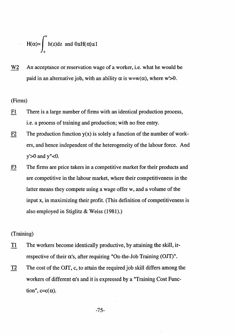
H(a)= I h(z)dz and 0<H (a)^l J 0
W2 An acceptance or reservation wage of a worker, i.e. what he would be
paid in an alternative job, with an ability a is w=w(a), where w’>0.
(Firms)
FI There is a large number of firms with an identical production process,
i.e. a process of training and production; with no free entry.
F2 The production function y(x) is solely a function of the number of work
ers, and hence independent of the heterogeneity of the labour force. And
y'>0 and y"<0.
F3 The firms are price takers in a competitive market for their products and
are competitive in the labour market, where their competitiveness in the
latter means they compete using a wage offer w, and a volume of the
input x, in maximizing their profit. (This definition of competitiveness is
also employed in Stiglitz & Weiss (1981).)
(Training)
T1 The workers become identically productive, by attaining the skill, ir
respective of their a 's, after requiring "On-the-Job Training (OJT)".
T2 The cost of the OJT, c, to attain the required job skill differs among the
workers of different a 's and it is expressed by a "Training Cost Func
tion", c=c(a).
-75-

(Information)
11 Every worker knows his own ability a and opportunity wage w=w(a).
12 Every firm knows h(a), c(a) and w(a) given a , but is not able to distin
guish one worker from another.
(Employment Contract)
El Employment contracts are negotiated in advance, last for one period and
specify a wage to be paid.
(2) The model
In this competitive labour market, as defined in F3, consider a representative
firm which faces a proportion of the aggregate labour supply. Let us construct
the supply of and demand for labour of the firm and then analyze the market
equilibrium.
(a) The supply of labour
Suppose there are n workers and m firms in the market. Then the supply of
labour available to the firm, xs say, is expressed as,
(n/m)h(z)dz = xs(w) (III-D
For the sake of simplicity, let us assume m=n, i.e. each firm faces a "normal
ized" potential labour supply. Note that since m and n are exogeneous to the
-76-

model, and in particular m is fixed due to no free entry (cf. FI), there would be
no loss of generality with this simplification.
This means in particular,
xs(w)=l when a(w )=l or equivalently w=w(l) (III-2)
xs(w)=0 when oc(w)=0 or equivalently w=w(0) (HI-3)
where a=a(w ) is the inverse of w=w(a), which exists by w'>0 (cf. W2). And
note that xs(w)>0 is a cumulative function. (See Fig.III-1 for how the supply
curve is constructed from w=w(a) and h(a))
w(a) h(a)w(a)
0
(a) (b)Fig.III-1
(b) The demand for labour
In constructing the demand function, note that a uniform wage is offered to the
workers of the heterogeneous ability since they are observationally indistinguish-
-77-

able. (For more extensive arguments on the uniformity of the wage, see Chapter
VI)
Being competitive, a firm can not control the supply quality of labour it faces
by varying the wage. However, it can control the quality by varying the wage
as it knows w(a), c(a), and h(a). Namely, the firm knows that a change in
wage affects the expected training cost c(a) through a change in the maximum
ability available.
And we can see that c ’(cc)<0 is a sufficient and not necessary condition for dc(a)- —7T -0- We will assume c’(a)<0 from here, emphasizing that it is not a dw(a)necessary condition for the model, as in the Weiss model. Therefore,
T3 c’(a)<0 V0<a<l
The firm is to maximize expected profit n with respect to w and xd, the demand
i.e. dc(oQ _dc(q) d a dw(a) d a dw(a)
where c(a)=
h(a) I [c(a)-c(z)]h(z)dz
(HI-5)[H(<x)]2w'(<x)
-78-

for labour, or equivalently a and xd, where
7C= py(xd)-c(a)xd-w(a)xd (III-6)
It should be noted that the difference between choosing (w,xd) and (a ,xd) as the
variables to maximize n is a practical one. In theory, w and c are functions of a
so that it would be more appropriate to use a and xd. In practice, however,
workers and firms are more likely to negotiate with w rather than with a . One
reason is that even if a worker is endowed with a certain a , a firm may not
accept it and in such a case the agreement is difficult to reach about the ability
endowment between the two. If they negotiate with w, on the other hand, there
is no ambiguity about w.
Here for an analytical purpose, we employ (oc,xd) instead of (w,xd). Then the
first order conditions give us
py'(xd)=c(a)+w(a) (III-7)
c'(oc)+w'(a)=0 (III-8)
It shows that a may be determined independently from (III-8), which then can
be substituted into (III-7) to obtain xd. Note that (III-7) resembles a convention
al demand function of a price-taking firm, since by rearranging it will give us,
w(a)=py'(xd)-c(a) (III-9)
-79-
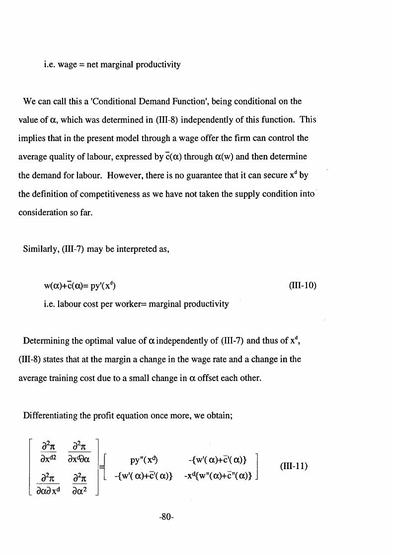
i.e. wage = net marginal productivity
We can call this a 'Conditional Demand Function', being conditional on the
value of a , which was determined in (III-8) independently of this function. This
implies that in the present model through a wage offer the firm can control the
average quality of labour, expressed by c(a) through a(w) and then determine
the demand for labour. However, there is no guarantee that it can secure xd by
the definition of competitiveness as we have not taken the supply condition into
consideration so far.
Similarly, (III-7) may be interpreted as,
w(a)+c( a)= py'(xd) (III-10)
i.e. labour cost per worker= marginal productivity
Determining the optimal value of a independently of (III-7) and thus of xd,
(III-8) states that at the margin a change in the wage rate and a change in the
average training cost due to a small change in a offset each other.
Differentiating the profit equation once more, we obtain;
d2n d2ndxd2 dx^a
d2n d2ndadxd d a 2
py»(xd) _{w»( oc)+c'( a)}
-{w'( oc)+c'( a)} -xd{w"(a)+c"(a)}(III-ll)
-80-
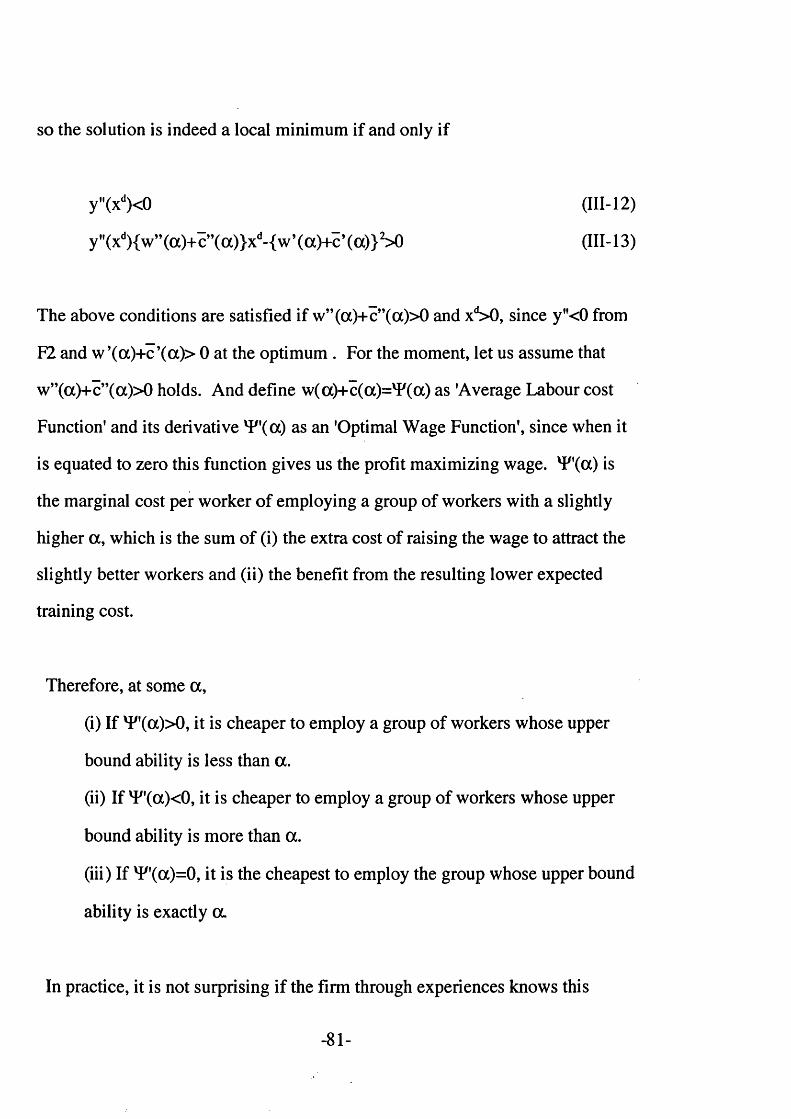
so the solution is indeed a local minimum if and only if
y"(xd)<0 (III-12)
y^x 'X w ’XaJ+c’XocWx^wXaJ+cXa)}2 (HI-13)
The above conditions are satisfied if w”(oc)+c”(oc)> 0 and xd>0, since y"<0 from
F2 and w ,(oc)+c’(ot)> 0 at the optimum . For the moment, let us assume that
w”(oc)+c”(oc)>0 holds. And define w (a)+c(a)=¥(a) as 'Average Labour cost
Function' and its derivative ¥'(oc) as an 'Optimal Wage Function', since when it
is equated to zero this function gives us the profit maximizing wage, ¥'(00 is
the marginal cost per worker of employing a group of workers with a slightly
higher a , which is the sum of (i) the extra cost of raising the wage to attract the
slightly better workers and (ii) the benefit from the resulting lower expected
training cost.
Therefore, at some a ,
(i) If ¥ '(a)> 0 , it is cheaper to employ a group of workers whose upper
bound ability is less than a .
(ii) If ¥ (a )< 0 , it is cheaper to employ a group of workers whose upper
bound ability is more than a .
(iii) If ¥'(00=0, it is the cheapest to employ the group whose upper bound
ability is exactly a
In practice, it is not surprising if the firm through experiences knows this
-81-
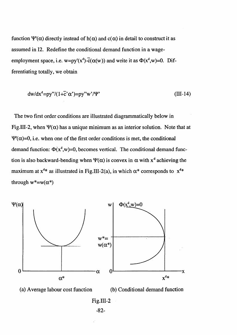
function ^'(oc) directly instead of h(a) and c(a) in detail to construct it as
assumed in 12. Redefine the conditional demand function in a wage-
employment space, i.e. w=py'(xd)-c(a(w)) and write it as O(xd,w)=0. Dif
ferentiating totally, we obtain
dw/dxd=py’7(l+c’a ,)=py”w7l /, (111-14)
The two first order conditions are illustrated diagrammatically below in
Fig.III-2, when xF(a) has a unique minimum as an interior solution. Note that at
'FCa^O, i.e. when one of the first order conditions is met, the conditional
demand function: O(xd,w)=0, becomes vertical. The conditional demand func
tion is also backward-bending when 'R(a) is convex in a with xd achieving the
maximum at xd* as illustrated in Fig.III-2(a), in which a* corresponds to xd*
through w*=w(a*)
w*=w(a*)
ar*
(a) Average labour cost function (b) Conditional demand function
Fig.III-2
-82-

So far we have assumed xF”(oc)>0 in order to derive these results. The techni
cal reason is that given that the optimal a exists s.t. lF,(oc)=0, ^ ( a ) > 0 ensures
that it is indeed the minimum. But what is the economic argument for 'F ”(oc)=
w”(oc)+c”(a)>0. Let us examine the two functions separately. As for the
reservation wage w(a), it is difficult to determine the sign of the second deriv
ative on a purely theoretical ground. Then, given w’(oc)>0, a linear function
would be the best approximation, i.e. w”(oc)=0. On an empirical ground, howev
er, we may refer to the Pigou paradox that the normally distributed ability,
which is a in our model,, generates a skewedly distributed earnings, which is w
in our model. This would mean w”(oc)>0, since the skewedness often described
as lognormal requires that a=logw and thus w”(oc)>0. We do not want to be too
optimistic about it, since the normally distributed ability is another controversial
issue. However, we accept the both arguments and assume w”(oc)>0. As c(a) is
a composite function of c(a) and h(a), they have to be treated separately. Giv
en c’(ot)^0 it is reasonably to assume c”(a)>0, since this means an increase of a
does not reduce c so much, as a becomes larger. If h(a) is “bell-shaped”,
c”(oc)>0 will be even more pronounced at higher values of oc, while at the low
values c”(cx)>0 might be less pronounced. However, on the whole, because of
c”(oc)>0, we assume c”(a)>0. Consequently, 'F ”(a)= w”(oc)+c”(a)>0. We
might point out, however, that “w”(a)>0 and c”(a)>0” is a sufficient but not
necessary condition.
Even if /”(a)= w”(a)+c”(a)>0 does not hold , all is not lost. In such a case,
-83-
as long as 'F(a) is a monotonic function, the solution may be found in a follow
ing way.
(1) If T 'X a)^ V a, the optimal ability to minimize 'F (a) is Gfc=0
(2) If T'XaKO V a, the optimal ability to minimize TXa) is a?=l
(3) If T'Xa^O V a, the firm would be indifferent among the workers.
And in these cases the corresponding conditional demand function: O(xd,w)=0
will be (1) downward sloping, (2) upward sloping or (3) vertical respectively.
This analysis shows that the adverse selection does not necessarily imply the
existence of an optimal wage. Adverse selection in this model means a negative
ly sloped c(a) for a positively sloped w(a) but this will not guarantee xF ’(cc)>0-
In fact any of the above cases of the monotonic T^a) could result with the
assumption of adverse selection. Hence, the shape of T^a) depends on the
relative shapes of w (a) and c(a). In particular, note that the assumptions w’>0
and c'<0 do not always guarantee the existence of a local minimum, i.e. the
existence of an optimal wage, at which vF’(a)=0, while it does guarantee an
existence of an adverse selection problem — adverse selection means a negative
correlation between w and c in this model. Hence, in this model adverse selec
tion does not necessarily imply an existence of a profit maximizing wage solely
determined by each firm, as in the case of the efficiency wage models. Note
also that the workers are not necessarily assumed to be all-round productive
this would mean c’(a)>0. But what we assume here is c’(a)>0, the adverse
selection condition and not c ’(oc)>0. Here the same logic as the numerical
example of (1-8) should apply. Technically as there is no need to inverse c(a),
-84-

we do not have to restrict this to a monotonic function.
Therefore, profit is maximized as long as the supply of labour is not binding,
by employing xd* workers at w*, for whom the expected training cost is c(cc*)
such that w*=w(a*). And this is equivalent to choosing a point on O(xd,w)=0
with the largest xd. Consequently the firm's demand for labour is a "single
point". In the conventional neo-classical competition, on the other hand, the
demand schedule is a locus because along the demand curve n monotonically
increases with x.
(3) The equilibrium
Here we analyze the market equilibrium of the present model in comparison
with a market equilibrium usually described in perfect competition with its
agents acting as mere price-takers. It can be seen that our equilibrium, though
competitive in its nature, does not always coincide with the market-clearing
equilibrium of a perfect competition. The reason is that in our model the firm
can obtain some information about the nature of the labour supply through an
"adverse selection" mechanism.
With our definition of competitiveness, at the equilibrium the aggregate supply
SL and demand DL would be
SL: Ns(w)=mxs(w)=nH(oc(w)) (III-15)

Dl : Nd(w) s.t. w+c(cx(w))=py,(Nd/m) (III-16)
where xs(w) is defined in (III-l).
For each firm the following holds at the market clearing equilibrium, where
(w+, x \ a +=oc(w+)) is its solution.
xs(w)=H(a(w)) (111-17)
py'(xd)=w+c(a(w)) (III-18)
xd=xs (III-19)
On the other hand, let (w*, x*, a*) be the solution to the firm's profit max
imizing problem, as derived in the previous sections. Then by our definition of
competitiveness, the solution of the present competitive model (w**, N**,
a**), where N**=mx** and cc**=oc(w**), is given by;
(I) if '(oO^O, then (w**, N**, a**) = (w+, N+, a +)
(II) if T'XoOcO, then (w**, N**, a**) = (w*, N*, a*)
We can interpret this in the following way : If 'Ff(cx+)>0, the market clearing
wage w (a+) is greater than the optimal wage w(oc*) so that at w(a*) the firm
can not secure the desirable number of workers and there will be an excess
demand, which will in turn raise the equilibrium wage as far as the market
clearing wage. If, on the other hand, xF '(a+)<0, the market clearing wage is
-86-
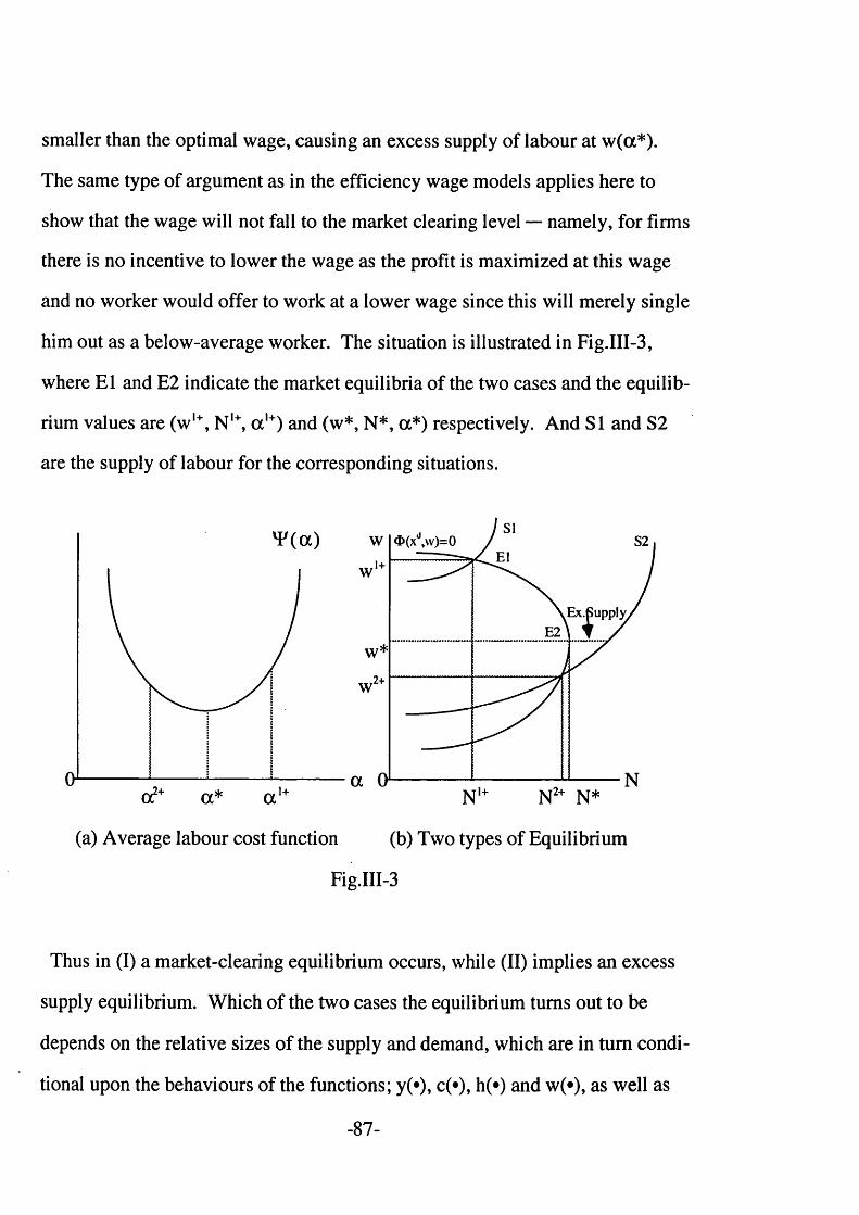
smaller than the optimal wage, causing an excess supply of labour at w(a*).
The same type of argument as in the efficiency wage models applies here to
show that the wage will not fall to the market clearing level — namely, for firms
there is no incentive to lower the wage as the profit is maximized at this wage
and no worker would offer to work at a lower wage since this will merely single
him out as a below-average worker. The situation is illustrated in Fig.III-3,
where El and E2 indicate the market equilibria of the two cases and the equilib
rium values are (wl+, N l+, a ,+) and (w*, N*, a*) respectively. And SI and S2
are the supply of labour for the corresponding situations.
Ex.Supply
E2
(a) Average labour cost function (b) Two types of Equilibrium
Fig.III-3
Thus in (I) a market-clearing equilibrium occurs, while (II) implies an excess
supply equilibrium. Which of the two cases the equilibrium turns out to be
depends on the relative sizes of the supply and demand, which are in turn condi
tional upon the behaviours of the functions; y(*), c(*), h(*) and w(»), as well as
-87-

upon p. These function reflect the aspects of the market from different angles.
While h(*) and w(«) reflect the characteristics of the society in which the eco
nomic mechanism operates, y(*) and c(*) reflect the idiosyncratic nature of the
production technology of the market and p that of a product market from which
the labour demand is derived.
Fig.III-4 shows various equilibrium outcomes for different VF(*). In each
figure the direction of arrows along the conditional demand function: O(xd,w)=0
indicates higher profit and E's the equilibrium points. To see how ¥ (•) affects
the behaviour of <b(xd,w)=0, one may refer to (111-14): dw/dxd= py"w74/' Mar
ket clearing occurs in (a) (b) (c) (d) and (f) corresponding to the equilibrium
condition (I), while excess supply occurs in (e) and (g), corresponding to the
equilibrium condition (II). (a) shows a demand function of homogeneous
labour force in the sense that the labour cost of every worker is equivalent from
the firm’s point of view. The equilibrium wage then becomes supply deter
mined. (b) includes cases of both homogeneous labour force in the sense of
perfect competition i.e. c=constant, and heterogeneous labour force i.e. c=c(a).
Note that being expressed in this way the homogeneous case does not seem
particularly different from other heterogeneous cases.
We might also mention another reason for a constant c(«) — it is possible that
the firm does not have enough information to construct c(») even if the labour
force is known to be heterogeneous, if the market is relatively new. In such a
case, we might expect that market-clearing is a temporary outcome, since when
-88-

and if more information on the heterogeneity is made known the equilibrium
may be characterized by an excess supply as in (e). In other words, more
information acquired by firms about the workers’ ability distribution means
unemployment. As this is involuntary unemployment, it is not good news for
the workers. However, as far as the firms are concerned, this does not imply
inefficiency, since they are able to recruit workers with better quality with this
information than otherwise.
With no information on supply quantity the aggregate demand price and
quantity would be where the quantity is maximum along the conditional de
mand function: O(xd,w)=0. In cases (a) (b) (c) and (f), this would means an
excess demand at the initial value of w. This will have to be revised since the
demand cannot be met and consequently each firm will have to raise its wage
offer to attract more workers until supply and demand match, (d) also is charac
terized by a market clearing equilibrium but its path to the equilibrium does not
require a tatonnement process since the demanders' initial position already
matches with the market clearing position.
On the other hand, in (e) and (g), excess supply would persist — there will be
no tatonnement process, since supply is not binding at the aggregate demand
price and hence this will be a market equilibrium. In (g), the equilibrium wage
will be set at the acceptance wage of the best worker i.e. w=w(l). Furthermore,
-89-

'Fta) w CDF S
w CDF
w CDF CDF w CDF
Ex.S
NO
Fig.III-4
where CDF: Conditional demand function S: Supply
E: Equilibrium 'F(a): Average labour cost function
-90-

no single unemployed worker can increase his probability of obtaining a job, by
reducing his acceptance wage i.e. by agreeing to reduce the economic rent,
since this would merely result in indicating to the firms that his value to them is
lower than the average worker's.
A level of the product demand expressed as a level of p affects the equilibrium
through a shift in the conditional demand function. A rise in p shifts this func
tion to the right, analogous to the case of perfect competition. In particular,
when the average labour cost function: 'F(a) has a local minimum, as in (c) (d)
and (e), a change in p could alter the nature of the equilibrium from excess
supply to market clearing and vice versa. Thus these two types of equilibrium
are compatible outcomes for a single market with firms of given characteristics.
So the competitive equilibrium may be characterized as either market-clearing
or excess-supply depending on the nature of the conditional demand function.
And there are some markets which possess both features: the equilibrium that
emerges depends on the level of the product demand.
In this chapter we have established the following :
Firstly, by introducing a heterogeneity in a , of which w and c are functions,
the assumption of all-round productive ability — that a good worker is a good
worker in all jobs — was relaxed. This helps to clarify that the assumption of
all-rounder productive ability, i.e. w ’(0)>O, is not a critical condition as stated in
-91-

Weiss (1980), for modelling an adverse selection mechanism. In our model, the
equivalent assumption is c’(a)<0 and even if we do not assume this the model is
not invalidated.
Secondly, the introduction of c(*) to reflect the heterogeneity among the work
ers for training gives a set of first order conditions consistent with marginal
productivity theory ( i.e. O(xd,w)=0: w(oc)+c(a)=py'(xs)) and with individual
labour cost minimization (i.e. 4/'(a)=w'(oc)+ c '(a)= 0 ) (See Fig.III-2) Unlike in
the efficiency wage models, this latter condition may not be satisfied for some
form of c(a), in which case the optimal wage does not exists.
Thirdly, excess supply was shown to be consistent with competitive equilibri
um. Furthermore, it was pointed out that the nature of production process i.e.
the training cost function, c, influences the existence of excess supply in the
same way as the product price does. It also showed that our competitive equilib
rium sometimes coincides with the orthodox type of competitive equilibrium
with market clearing feature.
Finally, recall that we have opted for this type of alternative models including
the family of efficiency wage models to explain the existence of firm's prefer
ence over workers. It might seem inconsistent that in our equilibrium, the
selection of Nd workers out of Ns workers when the supply exceeds the demand
at the equilibrium, is made at random, despite the firm's preference. But this is
not because the firm's preference does not exist over the Ns workers but because
-92-

the firm is unable to distinguish the workers once they have ’’self-selected".
Thus, there is naturally a tendency for the firms to improve the recruitment
process by some other measure of selection. As to the workers, those left out
are likely to be unemployed rather than taking an alternative job, since a non
negative economic rent is attached to the wage in the labour market, which
cannot be found in the alternative job.

CHAPTER IV : THE VALIDITY OF THE UNIFORM WAGE
So far in our analysis, we have been assuming that the uniform wage would be
paid to the workers of heterogeneous ability at the equilibrium. This is an
assumption common to the family of efficiency wage models.
On one hand, in practice it is not rare to observe a payment of a uniform wage
for performing an identical job even if the workers have different performance
levels. One may counterargue that the payment is uniform since each worker
would adjust his performance level so that the performance levels of all the
workers are equalized. But if it were the case, then one would not observe the
employer's preference among the potential workers, as pointed out at the begin
ning of Chapter I. Weiss (1980) refers to some empirical finding that "within
the same pay group there were very minor pay differences (among the workers)
On the other hand, the output of the most productive worker was often
more than three times as great as the output of the least productive worker
among fewer than 20 workers doing the same job with the same supervisor." In
other words, common practice seems to support the assumption of a uniform
payment to workers of different ability.
On the other hand, within the theoretical framework of a competitive analysis
one may argue that there exists a non-uniform wage payment that is preferred
by all the agents in the market and thus establishes itself as the equilibrium
-94-
contracts. To see this, recall the equilibrium we described in Chapter III. At the
equilibrium the workers of the ability range Q<a<a* were employed at
w*=w(a*). Now if a new firm enters and offers to the workers of the highest
ability among those attracted by w*, i.e. the workers with ability a* , a wage
marginally above the market wage, w*+£, say, then those workers would be
attracted by the offer and leave the existing firm. The new firm can do this
without reducing the profit by reducing marginally, for example, the wage offer
to the workers of the lowest ability, i.e. those with oc=0. For as long as there is
an excess supply at the equilibrium, this can attract those workers with the
lowest ability level. Thus this non-uniform contract is capable of disturbing the
uniform wage equilibrium. Of course, in the efficiency wage models, such a
possibility is usually ruled out with the assumption that the workers are indistin
guishable. This suggests that the uniform wage equilibrium may be disturbed if
some monitoring device is made available to distinguish the workers.
This chapter examines whether the uniform wage assumption has a theoretical
ly sound underpinning consistent with a competitive market framework. In
doing so, we will examine the arguments by Weiss (1980) and the arguments
based on the nature of OJT and then employ the concept of a pooling equilibri
um to verify the validity of the assumption.
(1) Possible Reasons for the Uniform Wage : the Weiss model
Weiss (1980) argues that there are several reasons why a firm may not offer,
-95-
instead, wages proportionate to productivity. The most obvious reason accord
ing to him is that the cost of precise information on the productivity of individu
al workers may exceed its benefit. This seems to be a rather intuitively appeal
ing argument. The paper, however, does not describe precise conditions under
which acquiring the information is not worthwhile for the firm. In fact the
natural extension of this line of argument is found in the literature on the infor
mational equilibrium, where there is a monitoring device with a cost on heter
ogeneous commodities in the market concerned. A large volume of works on
this topic is found in the analysis of an insurance market, of which Stiglitz &
Weiss (1976) is one offering a simple and yet clear argument. For the case of a
labour market, we find this type of argument in, for example, Guasch & Weiss
(1980) (1981) or (1982) or Clemenz (1986). In this chapter we will employ the
type of argument employed in Clemenz (1986) to verify the validity of the
uniform wage assumption.
Another reason for the uniform wage assumption in Weiss (1980) is that risk
aversion on the part of workers induces a wage payment not proportionate to
output or expected output at the equilibrium. The idea is that even if the produc
tivity of each worker is known, it does not necessarily imply that the value of
actual output can be known with certainty because of the demand uncertainty of
the product. However, the issue of adverse selection is essentially concerned
with asymmetric information between the firms and the workers, while output
uncertainty generates imperfect information to the agents of the both sides of a
labour market. Thus this argument does not depend directly on the heter-
-96-

ogeneity of the work force as the fundamental assumption of our model and
thus on the existence of the adverse selection in turn.
Weiss (1980) also argues that a payment proportionate to productivity or
expected productivity may not be realized as this scheme can cause friction
among workers, thereby lowering the morale of the workers. It needs to be
pointed out, however, that the moral issue is a question of workers' incentives
rather than of heterogeneous work force. While such a reasoning may be valid
for the incentive models of the efficiency wage hypothesis, this argument is not
appropriate here as the present model and the Weiss model alike are the adverse
selection models of and not the incentive models of the efficiency wage hypothe
sis.
(2) Uniform wage and OJT
According to Becker (1975), OJT may be either "firm-specific" or "general",
and this determines the incidence of its costs in a following manner. If OJT is
general, its cost will be paid by the worker as he collects the return for himself.
On the other hand, the cost as well as return of specific OJT are shared by the
two parties conditional upon the likelihood of labour turnover. Turning to our
model, if the training is general, then the workers would receive non-uniform
wages net of the training cost. Thus the training in our model that offers a
uniform wage must be specific.
-97-
There is some theoretical difficulty with this line of argument — namely,
according to this logic the training that each of the homogeneous firms offer s to
the workers is specific and yet has the identical training cost function c(®) One
can argue that some OJT cost may be paid by a firm even if it is not specific to
that firm. As was briefly mentioned in Chapter III, Manning (1994) also argues
for the uniform wage, or the company wage policy. He points out that the firms
do not use the information about worker characteristics in wage determination
and offer an individualistic wage policy, since it would be difficult to derive
such a complex policy that satisfies everyone in the labour market. Consequent
ly, the firms end up with providing, i.e. paying for, general training of the
workers. Stevens (1993) also shows the empirical support for and justifies
theoretically the idea that firms do invest in apparently general training of its
workers and are concerned with "poaching" at the same time. But again it is
difficult to determine the circumstance for such a wage offer within their ap
proaches.
In the next section, therefore, we develop the first argument for the uniform
wage assumption — the validity of the uniform wage payment as the equilibri
um contract when there exists a possibility of monitoring the workers.
(3) Pooling Equilibrium and Its Robustness
In order to simplify our argument, we specify our model to the case where
workers are characterized by one of only two ability types; each type has cor-
-98-

responding reservation wages and training costs. A similar type of model for
the adverse selection model of the efficiency wage hypothesis is found in Clem-
enz (1986). The basic result in his paper is that two types of equilibria are
possible in the labour market — a pooling equilibrium, in which the two types of
workers are offered a uniform wage contract, and a separating equilibrium with
monitoring, in which the two types of workers are employed with different
contracts from each other, making it a non-uniform wage contract. In the latter
case, the firms employ a monitoring device to distinguish the two types of
workers. And in both cases, the analyses examine the conditions in which
either or none of the equilibria exists.
The basic argument of this type of analysis is as follows. Given that firms in
the labour market are planning to offer the efficiency wage to all the workers
uniformly at the pooling equilibrium, the analysis asks whether there exists
some other labour contract preferred by all the agents in the market which offers
differentiated wages to the workers of different ability. In the latter type of
contract the firms are assumed to employ some monitoring device, which is
costly and inaccurate, in order to distinguish the workers. The particular form
of the non-uniform wage contract is not given, as it would depend on the specif
ic natures of the supply and demand conditions in the labour market. Rather, it
merely asks whether there exists any non-uniform wage contract based on the
monitoring mechanism, which is preferred by all the agents in the market and
thus invalidates the uniform wage contract as the equilibrium wage contract.
Having determined the conditions in which the pooling equilibrium does not
-99-
exist, the analysis then asks whether a separating equilibrium exists.
Here, to employ a similar type of argument for our model, we need to alter
slightly the assumptions made in Chapter III in the following way, where the
modified assumptions are indicated by primes.
(Workers)
W l1 There are two types of workers, Type I and Type II, whose ability levels
are and a 2, such that a ,< a 2, and their proportions in the total work
force are (3, and p2, such that P,+P2=l
W2' Acceptance or reservation wages of each type of workers, are and w2,
such that w,<w2.
(Firms)
FI There is a large number of firms with an identical production process,
i.e. a process of training and production; with free entry.
F2 The production function y(x) is solely a function of the number of work
ersers, and hence independent of the heterogeneity of the labour force.
And y'>0 and y"<0.
F3 The firms are price takers in a competitive market for their products and
are competitive in the labour market, where their competitiveness in the
latter means they compete using a wage offer w, and a volume of the
input x, in maximizing their profit. (This definition of competitiveness is
also employed in Stiglitz & Weiss (1981).)
-100-

(Training)
T1 The workers become identically productive, by attaining the skill, ir
respective of their a 's, after requiring "On-the-Job Training (OJT)".
T2* The cost of the OJT, c, to attain the required job skill differs for the two
types of workers are c, and c2, such that C j>c2.
(Information)
IT Every worker knows his own ability i.e. a , or a 2 and opportunity wage
i.e.w, or w2.
12* Every firm knows Pp Cj and ws of Type i workers, for i= 1,2, but is not
able to distinguish one worker from another.
13' The firm has a monitoring device which costs ji per worker and is
imperfect in such a way that n.. is the probability that it monitors a Type
i worker as a Type j worker i,j=l,2, with n n+II12= l, n ^ + n ^ l & n u,
n ^ i / 2 .
(Employment Contract)
El Employment contracts are negotiated in advance, last for one period and
specify a wage, or a set of wages to be paid according to the workers'
types.
(Treatment of risk)
RT Workers are risk averse and have an identical utility function of the von
-101-

Neumann-Morgenstem type, whose only factor is wage, i.e. u(w), such
that u’>0 and u"<0.
R21 The firms are risk neutral and maximize expected profits.
(a) Pooling equilibrium with a uniform wage contract
At w,, the firm attracts only Type I workers so that its expected profit is,
E^pytxM W j+c^x (IV-1)
while at w2, it attracts the both types of workers so that its expected profit is,
E(it)=py(x)-(w2+Plc,+P2c2)x (IV-2)
And w2 will be the equilibrium wage, if
W .+ C ^ W j+ ftc .+ p jC j
i.e. w2-w,<p2(c,-c2)
(IV-3)
(IV-3)’
provided that there exists an excess supply of labour. We define this as a pool
ing equilibrium as with this wage offer the firm is able to attract the both types
of workers with the same condition. In terms of our continuous model of Chap
ter III, this would be equivalent to saying that at w2=w(a2), w (a)+c(a) is min
imized or equally w '(a)+cf(a)=0
-102-
(b) A non-uniform wage contract as an alternative
Now introduce a two-wage contract WM=(w,,w2), with an imperfect and costly
monitoring device, where a worker monitored as Type I receives w, and a
worker monitored as Type II receives w2. Then the uniform wage contract may
be upset if;
(i) one or the both types of workers prefer this contract to the uniform
wage contract.
& (ii) the firm can generate profits with this contract that are at least as
large as with the uniform wage contract.
The first condition implies that at least one of the following conditions is met.
uf e ) <^ i iu(w i)+ ^ i 2u(w2) for Type I workers (IV-4)
u(w2)< n 2Iu(w,)+II22u(w2) for Type II workers (IV-5)
Fig.IV-1 illustrates this set of constraints with the assumptions that workers are
risk averse and n n, Il22>l/2. The curves I and II are the indifference curves of
the two types of workers i.e. (IV-4) and (IV-5) with equality, so that (IV-4) and
(IV-5) hold to the right of the indifference curves I and II respectively. Our
interest lies in the area below the 45° line since w,<w2. Any contract in the
area A is preferred by the both types of workers to the uniform wage contract
indicated as W , while any contract in the area B attracts Type II workers only
away from the uniform wage contract W . And no contract in the area C can
attract any worker away from the uniform wage contract. The both curves are
-103-

0 w2 w2
convex to the origin due to the assumption of the risk-averse workers, while the
indifference curve I is drawn above the indifference curve II to the right of the
45° line because at W p the absolute slope of the indifference curve I, n i2/ n n is
smaller than the absolute slope of II, I l 22II\2X because of n ,p IX ^ l/2 . As for
the second condition, the firm's expected profit depends on the type or types of
workers it can attract by the wage contract. First, if the firm can attract the both
types of workers, which implies that the contract must lie in the area A, its
expected profit would be
7cM=py(x)-{(pln l]+p2n2,)wl+(pln,2+p2n22)w2+p1c1+p2c2}x-^x (iv-6)
where P ^ is the proportion of the workers of Type i monitored as Type j over
the whole labour force, with i,j=l,2. It is assumed here that the required labour
demand x is satisfied by the labour supply. Here the second condition may be
expressed as,
-104-

(Pin M+P2n 2|)Wl+(Pin i2+P2n 22)W2+PlCl+P2C2-|X5W2+P|C|+p2C2 (IV-7)
i.e. ( p ,n ll+p2n 21)w1+(p1n l2+p2n 22)w2sw 2-n (iv-71)
However, we can show that such a contract does not exists.
(Proposition IV-1) There is no WM=(w,,w2) that satisfies (IV-4) (IV-5) and
(IV-7') simultaneously.
(Proof)
The risk-averse workers means
uf e ) <n„u(w1)+ni2u(w2)<u(niIw1+ni2w2) for Type I workers
u(w2)<n 21u(w1)+n22u(w2)<u(n2Iw ,+II22w2) for Type II workers
and they mean in turn
w2<n, ,w,+ni2w2 for Type I workers (IV-4’)
w .cIT^w.+n^w, for Type II workers (IV-5')
Now with (IV-4') and (IV-5'), the right hand side of (IV-7') will be such that
(Pini,+p2n2|)Wl+(Pini2+P2n22)W2>W2>W2-|i
which contradicts (IV-7')
Q.E.D.
-105-
Next, if the firm attracts Type II workers only, which implies that the contract
must lie in the area B, the expected profit would be
7tM=py(x)-(n2|w|+n22w2+P2c2)x-|!x (IV-8)
assuming that the required demand x is satisfied by the supply of Type II work
ers alone. And this means that the second condition is expressed as,
Here we can show that such a contract does not exist if Pj(c,-c2)<p,
(Proposition IV-2) There is no WM=(w,,w2) that satisfies (IV-5') and (IV-91) if
p,(c,-c2)<^.
(Proof)
Given Pj(c,-c2)<ii, (IV-9') implies n^Wj+II^Wj^cw^. However, this contra
dicts (IV-51), the condition derived from the risk-averse Type II workers.
As for the area C, there could be no production as no worker can ever be
attracted away from the uniform wage contract Wp=(w2,w2).
n2,wi+n22w2+P2c2-mw2+PIc1+P2c2i.e.r^w, +n22w2 w2+p, (c, ■-c2)- \i (IV-9')
(IV-9)
Q.E.D.
-106-
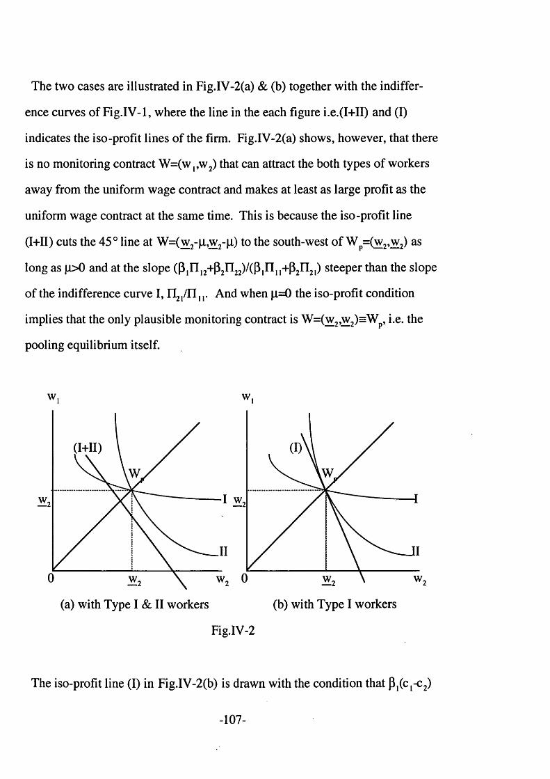
The two cases are illustrated in Fig.IV-2(a) & (b) together with the indiffer
ence curves of Fig.IV-1, where the line in the each figure i.e.(I+II) and (I)
indicates the iso-profit lines of the firm. Fig.IV-2(a) shows, however, that there
is no monitoring contract W=(w,,w2) that can attract the both types of workers
away from the uniform wage contract and makes at least as large profit as the
uniform wage contract at the same time. This is because the iso-profit line
(I+II) cuts the 45° line at W=(w2-|i,w2-|i) to the south-west of W p=(w2,w2) as
long as j l i >0 and at the slope (Pin i2+P2n22)/(Pin il+P2n21) steeper than the slope
of the indifference curve I, FL^/IIn. And when p=0 the iso-profit condition
implies that the only plausible monitoring contract is W=(w2,w2)=Wp, i.e. the
pooling equilibrium itself.
w, w,
(I+II)
— 2
2 '
(b) with Type I workers(a) with Type I & II workers
Fig.IV-2
The iso-profit line (I) in Fig.IV-2(b) is drawn with the condition that P ^ - c ^
-107-
=p,. Note here that the iso-profit line (I) is tangential to the indifference curve II
at W . (I) would shift to the left if P,(c,-c2)<|i and to the right if p,(c,-c2)>|i. As
in the above case, therefore, no alternative monitoring contract exists if P,(c,-c2)
3 1 .
Thus together with (IV-3?), the condition for w2 as the pooling equilibrium, the
uniform wage contract exists as the equilibrium contract if,
^ - ^ c p iC e ,- ^ ) & (IV-10)
In (IV-10), P^Cj-Cj) is the difference in the average training cost per worker
between the two uniform wage contracts, i.e. w, and w2, while P,(c,-c2) is the
difference in the average training cost per worker between the uniform wage
contract Wp=(w2,w2) and an monitoring contract W M=(w,,w2) which attracts
only Type II workers. Thus these inequalities simply state that in order for the
uniform wage offer w2 to be an equilibrium,
(i) for the two uniform wage offers, w, and w2, the difference in average
training cost per worker must be greater than the difference in the wage
cost per worker.
(ii) for the uniform wage offer w2, or Wp=( w2,w2) equivalently and a
monitoring contract W=(w,,w2), the reduction in average training cost per
worker when the latter is considered must not exceed the cost of mon
itoring.
-108-
In terms of the values of |i, (3,, c,, c2, w f, and w2, this means that the uniform
wage assumption is valid when,
(i) (I is sufficiently large, i.e. monitoring cost is large
(ii) (3, is sufficiently small, i.e. Type II is a large group
(iii) c,-c2 cannot be too large or too small, i.e. it needs to be large enough
to make w2 as the pooling equilibrium rather than w,, but at the same
time it needs to be not too large to make an alternative contract with
monitoring upset w2 as the equilibrium wage.
This result helps to clarify the first argument by Weiss (1980) for the assump
tion of uniform wage that the cost of precise information on the productivity of
individual workers may exceed its benefit. While (i) states that acquiring the
information may not be worthwhile when its cost is high, (ii) states that a gain
in monitoring is small because Type II workers already constitute a large part of
the labour force without monitoring, (iii) states that a gain in monitoring is
small because the training costs of the two groups of workers are not large
enough to offset the cost of monitoring. But at the same time if it is too small
this could make the wage offer w, more profitable than w2 to the firm.
At this point, it needs to be mentioned that the next step in a standard informa
tional equilibrium literature is to see if any other type of equilibrium exists
when the pooling equilibrium fails to exists. A separating equilibrium is the
alternative equilibrium, at which there is a set of contracts, W,=(wn,w12) and
W2=(w21,w22), say. And each contract is preferred by one type of workers. We
-109-

do not go further into the discussion on the separating equilibrium here, since
our aim of this chapter is to verify whether the assumption of uniform wage is a
valid one by examining the conditions in which the pooling equilibrium with
the wage offer w2 is likely to occur.
(4) An Application To The Case Where Ability Is Continuous
The argument for the continuous ability case is far more complex and the
intuitive reasoning with a help of figures such as Fig.IV-1 & 2 for the two-
ability case discussed above is no longer applicable. In this section I merely
intend to show that the fundamental approach would remain unchanged when
the two-ability case is generalized to the continuous case.
When the heterogeneity of the workers is assumed as in Chapter III, the alterna
tive monitoring contract would take a form WM={co(a)} with 0 < a^ l. Assum
ing that the labour demand were fulfilled by Type a* workers alone, (IV-9), i.e.
the condition that it is worthwhile for a firm to offer this monitoring contract,
may be expressed as,
where II(a*,cx) is the probability of a Type a* worker being monitored as Typera , such that I I I(a* ,a )d a = l and 00(a) is the wage offer to Type a workers.
However, the assumption that all the labour demand would be satisfied by Type
n(a*,a)co(a)da+c(a*)+(x<w(a*)+c(a*) (IV-11)
-110-

a workers clearly is not plausible as the supply of labour of Type a workers
alone is zero in the continuous case. Rather, the left hand side of (IV-11)
should be taken as the lower bound of the average training cost, for employing
the workers with a< a* would result in an increase in the average labour cost.
Of course, W M={co(a)} also has to meet the condition that this will only attract
Type a* workers only away form the pooling contract with the uniform wage
w*=w(a*). Let us assume that this is also met.
Then no monitoring contract can attract away the workers from the pooling
contract if the lower bound of its average labour cost, i.e. wage cost and training
cost per worker, is greater than the corresponding cost for the pooling contract.
By rearranging (IV-12), we can obtain the analogous condition to (IV-9’) as,
Here the same argument as Proposition IV-2 may be applied to state that the
pooling equilibrium exists if c(cc*)-c(a*)<ji. And this holds if,
(i) |i is sufficiently large
(ii) c(oc*)-c(oc*) is sufficiently small
Here the first condition is identical to the case of the two-type ability case. The
second condition says that the difference between the average training cost
n(a*,a)w(a)da+c(a*)+|i>w(oc*)+c(a*) (IV-12)
n(cc* ,a)co (a)da>w(a*)+c(a*)-c(a*)-p (IV-13)
among the workers with Q^a^a* and the training cost of the workers with a* is
very small. It is easy to deduce here that this difference is small when c(a) is
relatively flat since this would imply that c(a) does not differ much from c(a)
for all values of a and for a* in particular, and when the workers are concentrat
ed at the higher values of a since this would imply a generally low level of
c(a). And again these conditions are the same as the conditions derived for the
two-ability case.
In this chapter we have established the following;
First, we examined the reasons put forward by Weiss (1980) for the validity of
the uniform wage assumption in the adverse selection model of the efficiency
wage hypothesis. Of the three reasons we examined, it was concluded that the
only valid reason was the first argument that the cost of precise information on
the productivity of individual workers may exceed its benefit. However, it was
pointed out that there is a need to offer a more theoretically rigorous argument.
The other two reasons were ruled out as they are not necessarily based on the
adverse selection mechanism.
Secondly, the model in Chapter III was slightly modified to apply the argu
ment in the informational equilibrium literature to offer the more theoretical
approach of the Weiss's first argument. Using a two-type ability worker model,
our equilibrium was established and defined as the pooling equilibrium.
-112-

Thirdly, the robustness of the pooling equilibrium was discussed against other
alternative wage contracts with imperfect and costly monitoring. And it was
concluded that the pooling equilibrium exists and thus the uniform wage equilib
rium derived in Chapter III is valid when the monitoring cost is high, the propor
tion of the workers with high ability is high, and/or the training cost difference
among the workers of different ability level is neither too small or too large.
And finally, an attempt was made to generalize these results to the case of the
continuous ability, in which it was found that the same line of argument may be
applied and that the conditions for the pooling equilibrium to be robust were the
same as in the case of the two-ability worker case.
-113-
CHAPTER V : TWO-PERIOD MODELS OF TRAINING
In this chapter, we add one more period to our analysis of the training model
This would be a reasonable extension, as training is essentially a dynamic issue.
However, the main purpose of this extension here is to contrast our training
model of heterogeneous labour with the adverse selection models based on the
efficiency unit assumption such as Weiss (1980), so that the model is kept as
simple as possible. The discussions proceed in three steps. First, the general
framework of the model is briefly explained in relation to the Weiss model as
well as other training models. Then a two-period model is introduced, in which
the firm maximizes its profit for each period. And finally, we consider the
two-period model with the firm maximizing the present value of the profit
stream.
(1) The Basic Framework
The basic framework of the model remains unchanged in this two period case.
Thus in the period I the workers receive the training alongside production. In
the period II the workers are assumed to become equally productive and need
no more OJT. Thus in the period II the firm does not have preference among its
work force, while the Weiss’ firm was never indifferent about its work force. In
fact the assumption in the adverse selection model that the firm never learns
about the heterogeneous productivity of its workers is often called into question.
-114-
This becomes even more questionable when the model has to operate several
periods. Besides, it would be difficult to model the upward-sloping wage
profile within the Weiss’ framework.
Indeed, one of the main features of the labour models with specific training
See, for example, Donaldson & Eaton (1976), Nickell (1976), Ohashi (1983),
or Felli & Harris (1996), is the derivation of an upward-sloping wage profile.
The firm invests in workers by training them in the first period to receive the
return in the second period. However, if the worker quits it can not procure the
return. As a result the firm sets the wage lower in the first and higher in the
second periods, to prevent the premature quitting by the trained workers. Note
that this OJT has to be specific for this result to hold, since the standard view is
that the firm is not going to pay for general training. The incidence of training
cost was discussed with the survey on training models in Chapter II. As pointed
out, the distinction between general training and specific training is not the core
assumption in some of the recent models such as Stevens (1994c) and Acemo-
glu (1997).
Most of the training models assume homogeneous labour and consequently
there is no adverse selection, let alone the existence of unemployment. The
exception is Salop & Salop (1976), who assume that the quit rate is a negative
function of wage offer. When new workers are recruited in place of the quitters,
there is a fixed cost of training them. There is an adverse selection in the sense
that the higher the wage offer is the more reliable the type of labour will be
-115-

reducing the average quit rate and hence the lower the total training cost will be.
Hence the firm has to weigh the wage cost and the training cost, to determine
the wage offer. Salop & Salop (1976)’s modelling of a labour market with
training and heterogeneous aspects is very similar to ours. However, the heter
ogeneity is not as explicit as ours with c(*) and thus can not relate easily the
degree of heterogeneity and the nature of equilibrium.
We assume that the firm always “pays” for the training whether it is general or
specific. This is because with heterogeneous labour it is costly for the firm to
determine the training cost of each worker to charge them individually. Instead,
the firm prefers to pay the total training cost. This assumption is supported by
the descriptive arguments by Weiss (1980) and Manning (1994) as well as the
pooling equilibrium analysis in Chapter IV that monitoring of the individual
training cost itself is costly because of the heterogeneity of the work force.
Acemoglu (1997) argues that the training is general and yet the training firms
do pay for it in some countries where the level of training is high such as in
Germany and Japan and thus sets up his model accordingly. However, it goes
without saying that the real incidence of the training cost is likely to be shared
between the two, as in a typical tax incidence argument. In the multi-period, the
nature of training plays an important role in determining the opportunity wage
of the post-training periods. This is because the more general the training is the
higher the productivity in an alternative job will be. Thus his opportunity wage
i.e. the wage he can demand in the alternative job will rise with the degree of
generality of the training In the present model we will assume that the training
-116-

has both general and specific elements in such a way that the opportunity wage
of the trained worker in the post-training period is w(a,*)+kc(a,*), where
0<k<l is a parameter of general applicability of the training. Thus if k=0 it is
completely specific, while k=l implies a fully general type of training.
(2) Case I : Optimizing At Each Period
First, assume that every firm maximizes the profit in the each period. Then for
the period I, the firm maximizes the profit n with respect to the employment
level x, and the ability index a ,, with the subscript signifying the period I,
rc pyO MwCcg+cCogix, (v-i)
This is equivalent to the optimization problem in Chapter III of the single
period case and the corresponding first order conditions are
d7c1/dx1=py’(x1)-[w (a1)+c(a1)]=0 (V-2)
drc/da^-Iw^a^+cXc^XIXpO (V-3)
Then the solution {0Cj*, Wj*, Xj*} could cause either excess supply or market
clearing in the labour market, depending on the supply availability. As for the
incidence of the training cost, (V -l) simply repeats our assumption that the firm
pays for the training i.e. c(a,)x, irrespective of the type of training. Also note
that from (V-2) the wage is equated to the net marginal productivity, i.e. net of
-117-

training cost, and consequently there is no discrepancy between the wage and
the marginal productivity. This point is worth mentioning since the discrepancy
is a much-discussed issue in the training literature in relation to the labour
turnover.
In the period II, with x,* workers already needing no more training the firm
maximizes the profit n 2 by choosing the levels of wage offer w2, through deter
mination of a 2, and of employment x2, given oq* and x,*, where
7c2=py(x2)-[w(a2)+c(a2)](x2-x1*)-[w(a,*)+kc(a,*)]xI* (V-4)
The second term refers to the labour cost i.e. wage and training, of new workers
and the third to the wage cost i.e. the opportunity wage, of the existing workers.
And the first order conditions are,
djt2/dx2=pyXx2)-[w (a2)+c(a2)]= 0
drc2/d a 2=-[w’ ( a 2)+c’ (a 2)]x2= 0
which are in fact identical to the first order conditions for the period I.
Thus, a 2*=a,*, w2*=w,*, and x2*=xt* and the firm repeats his action in the
period II. This rather trivial result is due to the fact that the reduction in the
total cost of training x}* workers in the period II i.e. c(a,*)x1*, is a fixed sum by
the time x,* is decided and thus does not affect the firm’s decision in the period
-118-
(V-5)
(V-6 )

II. (V-6 ) implies that the optimal wage is unaffected and neither is the best
group of workers for the firm. And this in turn means that with (V-5) the de
mand for labour remains as before. This generates an upward-sloping wage
profile over the periods with w,*=w(a,*) and w2*=w(a,*)+kc(a,*). And the
profile becomes steeper as the degree of generality i.e. k rises. This is true as
long as the excess supply condition holds. Note also that there will be no more
recruitment as long as 0<k<l, since for the period II the existing worker costs
w2*=w(a,*)+kc(a1*), while the new worker would cost w2*=w(a,*)+c(a1*),
and w (a,*)+kc(a1*)<w(a1*)+c(a1*). When k=l, on the other hand, the firm
becomes indifferent between the two groups of workers in the period II. For
example, the firm could lay off all the existing workers and employ totally new
labour force. This can be interpreted as not following a seniority rule, with the
seniority rule being defined as giving a priority of employment to the longer
serving workers. It goes without saying that when 0<k<l the rule holds as no
new worker is employed. If more workers are needed in the period II due to an
exogeneous increase in the product demand, the firm will still seek for the same
type of workers by offering the same optimal wage as long as the excess supply
exists. The new workers would then receive w ^ * ) in the period II, i.e. what
the existing workers received in the period I, while the latter will have a wage
increased to w(a,*)+kc(a,*).
We may contrast this result with how the Weiss model would perform in the
two period case. If the profit maximization is done at each period as in our
model, the Weiss model would produce the identical equilibria in the two
-119-
periods. As a consequence, the wage profile will always be flat and there will
be no seniority rule concerning who is to employ first. Considering the fact that
the formation of human capital over time may play an important role in the
operation of a labour market, these results require some justifications. Further
more, the Weiss’ firm would remain ignorant about the productivity of each
worker over two periods i.e. even after the production is completed. It is dif
ficult to imagine that the firm continues to turn the blind eye to the information
on the true productivity of the heterogeneous workers.
(3) Case I I : Optimizing Over Two Periods
So far the firm was assumed to act as a profit maximizer in each period. How
ever, it is probably more realistic to assume that it maximizes the profit stream
over time, as it takes time to generate the return on the training. Therefore, the
firm would maximize, by setting the wage offer {w,, w2} and the employment
levels x, and x2, the present value of the profit stream PV(7t),
PV(K)=py(x,)-[w1+c(a)]x1+ (l+ r)l[py(x2)-w2x2] (V-7)
where r is the discount rate. Before we move on to the firm’s optimization, note
that it has to offer an attractive wage profile to the workers as well as max
imizing its own present value. We tackle this by two steps. First list up all the
wage profiles {Wj,w2} that gives the same labour cost to the firm. Then the
worker’s utility maximizing wage profile is derived given some constraints on
-120-

the profile. As c(a) appears in (V-7), w , & w 2 must attract those workers with
the ability below a , one of the wage profiles being w,=w(a) & w 2=w(a)+kc(a).
Then the firm could give any other wage profile as long as labour cost remains
unchanged. Therefore, for the given values of a , x,, and x2, w, & w 2 will satisfy
the following condition,
[w1+c(a)]xl+(l+r)'lw2x2=[w(a)+c(a)]x,+(l+r)'1[w(a)+kc(a)]x2 (V-8 )
i.e. w ,x1+(l+r)‘,w2x2=w(a)xI+ (l+ r)1[w(a)+kc(a)]x2 (V-8 )’
Assume further that there is no turnover, i.e. no worker quits or is laid off, and
thus x,=x2=x. A typical specific training model — see, for example, Hashimoto
(1981), Nickell (1976), Donaldson & Eaton (1976), or Ohashi (1983), would
assume the turnover rate to be determined within the model. And in particular,
a quit rate is generally assumed to be a positive function of the period II wage,
with the rationale that the partly deferred payment reduces their incentive to
quit, and this is the reason for the upward-sloping wage profile in general. In
the present model, we do not have to worry about the deferment since the
productivity rises over time at the firm as well as outside in our model as long
as k>l. On the whole, it is not intuitively appealing to assume that the firm sets
the quit rate above zero by setting the wage profile, unless this is done to screen
the workers.
This assumption sets ranges to the values of w, & w2. First, observe that
x,=x2=x changes (V-8 )’ to,
-121-

wI+(l+r)‘,w2=w (a)+(l+r) '1 [w(a)+kc(a)] (V-8 )”
Suppose now that w,>w(a). Then by (V-8 )”, w2<w(a)+kc(a). The workers
would find it to their benefit to quit the firm at the end of the period I, since they
can earn w(a)+kc(a) elsewhere by definition. Thus, in order to keep the trained
workers for the period II, the firm needs to set the wages to the ranges of
w,<w(a) & w 2>w(a)+kc(a) (V-9)
If, on the other hand, the wage in the period I is too low, the workers might
find it difficult to believe the firm’s no-layoff policy. Thus the firm has to offer
a wage profile which shows that laying off the trained workers to replace them
with the new workers is more costly than keeping the existing labour force and
thus it has no intension to do so.
i.e. w 1+ c(a)+ (l+ r)1[w(a)+c(a)]>w 1+c(a)+(l+r)'1w2 (V-10)
i.e. w(a)+c(a)>w2
And with (V-8 )” , the workers believe that there is no lay off, if
w ,>w(a)-[(l-k)/(l+r)]c(a) & w 2 w(a)+c(a) (V-l 1)
(V-9) and (V-l 1) together set the ranges of wt & w2 as,
-122-

w(a)-[(l-k)/(l+r)]c(a)^w ,^w (a) & w(a)+kc(a)^w 2 w(a)+c(a)
(V-12)
a quick glance at which tells us W j<w(a)<w(a)+kc(a)<w2, i.e. w,<w2, with the
equality holding when k=0. So the wage profile is either flat or upward-sloping.
Given (V-12), the firm would set the wages to attract the workers. If the
workers are assumed to be risk-averse following the analysis of Chapter V, the
firm needs to offer a wage profile that maximizes the present value of the work
er’s utility, PV(U)
PV(U)=u(wI)+(l+r)_lu(w2)
s.t. w ,>w (a)-[(l-k)/(l+ r)]c(a): Xx (V-13)
w ,<w (a): X2 (V-14)
W j+Q+ryV^wCaHG+ry’lwtoO+kcCa)]: p (V-15)
where the X} and are the multipliers for the w , constraints on the lower bound
and the upper bound respectively, while p is for the iso-labour cost condition of
the firm so that this with (V13) & (V-14) will set the lower and the upper
bounds of w2. Then the Lagrangian L is;
Z^=u(w1)+(l+r)'1u(w2)+X,1[w1-w(a)-[(l-k)/(l+r)]c(a)]+A,2[w1-w(a)]
+p[w (a)+(l+r) 1 [w^+kc^oOJ-Wj-U+r) '1 w2] (V-16)

Note that the multipliers are set so that they become either zero if the constraint
is not binding or positive if binding. In particular, \ and \ will have to satisfy
one of the three conditions ; (1) ^ > 0 & A,2=0, i.e. Wj=w(a)-[(l-k)/(l+r)]c(a),
which means from (V-8 )” , w2=w(oc)+c(a), (2) A,j=0 & A,2=0, i.e. w (a)-[(l-
k)/(l+r)]c(a)<w,<w(a), which means from (V-8 )” , w(a)+kc(a)<w2<
w(a)+c(a), or (3) A,,=0 & ^ 2>0, i.e. w,=w(a), which means from (V-8 )” ,
w2=w(a)+kc(a) Then the first order conditions imply the following,
as well as the constraints. Eliminating p from (V-17) and (V-18), we obtain,
uXw^-uXWjHXj-A^O
If (1) ^ > 0 & ^ 2=0, then u ’(w,)-u’(w2)<0 and thus w t>w2. This is not consistent
with (V-12). If (2) ^ = 0 & X,2=0, then u^w ^-uX w ^O and thus w,=w2. But it
only holds when k=0. It turns out (3) ^= 0 & X2>0 is the solution, when
W j=w(oc) and w2=w(a)+kc(a) from (V-8 )”.
Fig.V-1 illustrates the optimization on the w,-w2 wage space. The negatively-
sloped line AD indicates the firm’s iso-wage cost line (V-8 )”, while the segment
BC on the line AD is derived from the no-tumover condition (V-12). Note that
uXw^+^-^-p^O
u ’(w 2) -p = 0 (V-18)
(V-17)
-124-
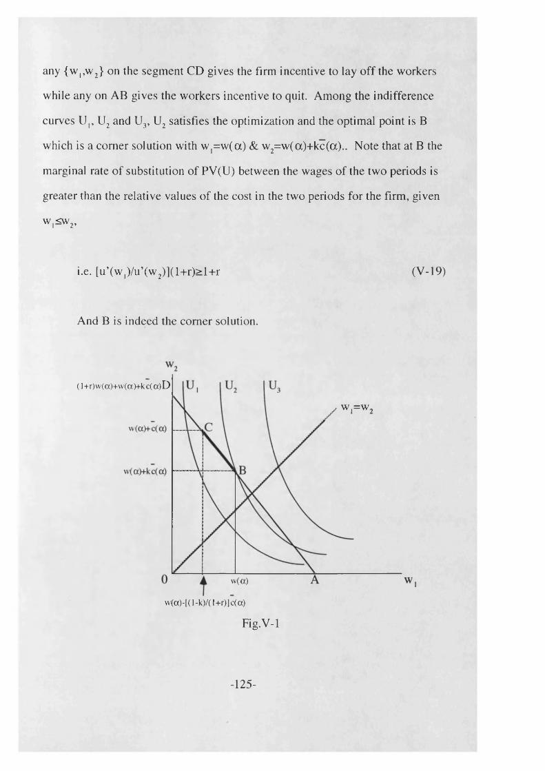
any {w ,,w 2} on the segment CD gives the firm incentive to lay o ff the workers
while any on AB gives the workers incentive to quit. Among the indifference
curves U,, U 2 and U3, U 2 satisfies the optimization and the optimal point is B
which is a comer solution with w ,= w (a) & w2=w (a)+kc(a).. Note that at B the
marginal rate o f substitution o f PV(U) between the wages o f the two periods is
greater than the relative values o f the cost in the two periods for the firm, given
w,<w2,
i.e. [u’(wj)/u’(w 2)]( 1 +r)> 1 +r (V-19)
And B is indeed the comer solution.
( l+ r)v v (a )+ \v (a )+ k c (a )D
w ,=w
w (a )
v v (a )-[(l-k )/( l+ r)]c (a )
Fig.V-1
-125-
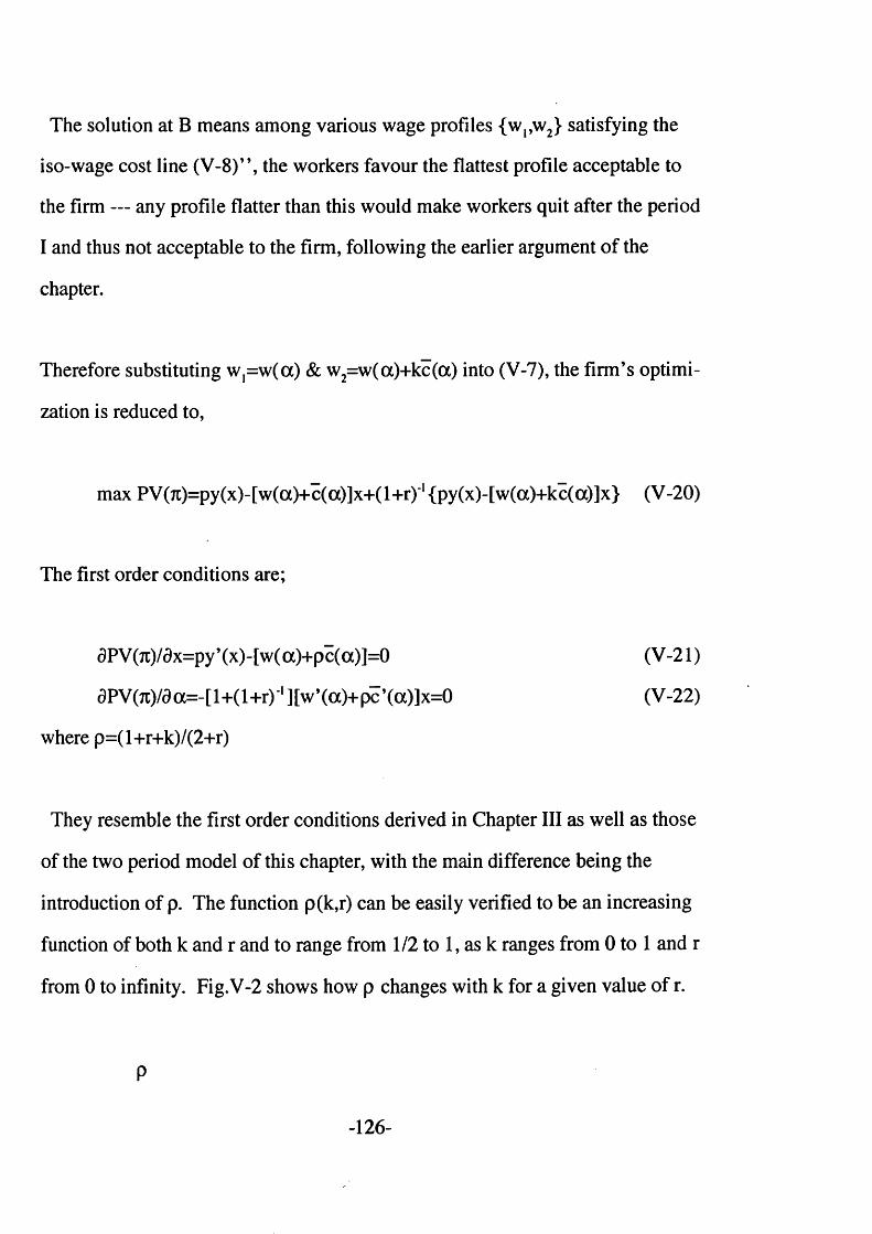
The solution at B means among various wage profiles {w,,w2} satisfying the
iso-wage cost line (V-8 )” , the workers favour the flattest profile acceptable to
the firm — any profile flatter than this would make workers quit after the period
I and thus not acceptable to the firm, following the earlier argument of the
chapter.
Therefore substituting w,=w(a) & w2=w(a)+kc(a) into (V-7), the firm’s optimi
zation is reduced to,
max PV(7c)=py(x)-[w(a)+c(a)]x+(l+r) '1 {py(x)-[w(a)+kc(a)]x} (V-20)
The first order conditions are;
dPV (rc)/dx=py ’ (x)- [ w( a)+p c( a)]=0
dPV (7t)/d a=- [ 1+(1 +r) 1 ] [w ’ (a)+ pc ’ (a)] x=0
where p=(l+r+k)/(2 +r)
They resemble the first order conditions derived in Chapter III as well as those
of the two period model of this chapter, with the main difference being the
introduction of p. The function p(k,r) can be easily verified to be an increasing
function of both k and r and to range from 1 /2 to 1 , as k ranges from 0 to 1 and r
from 0 to infinity. Fig.V-2 shows how p changes with k for a given value of r.
P
(V-21)
(V-22)
-126-
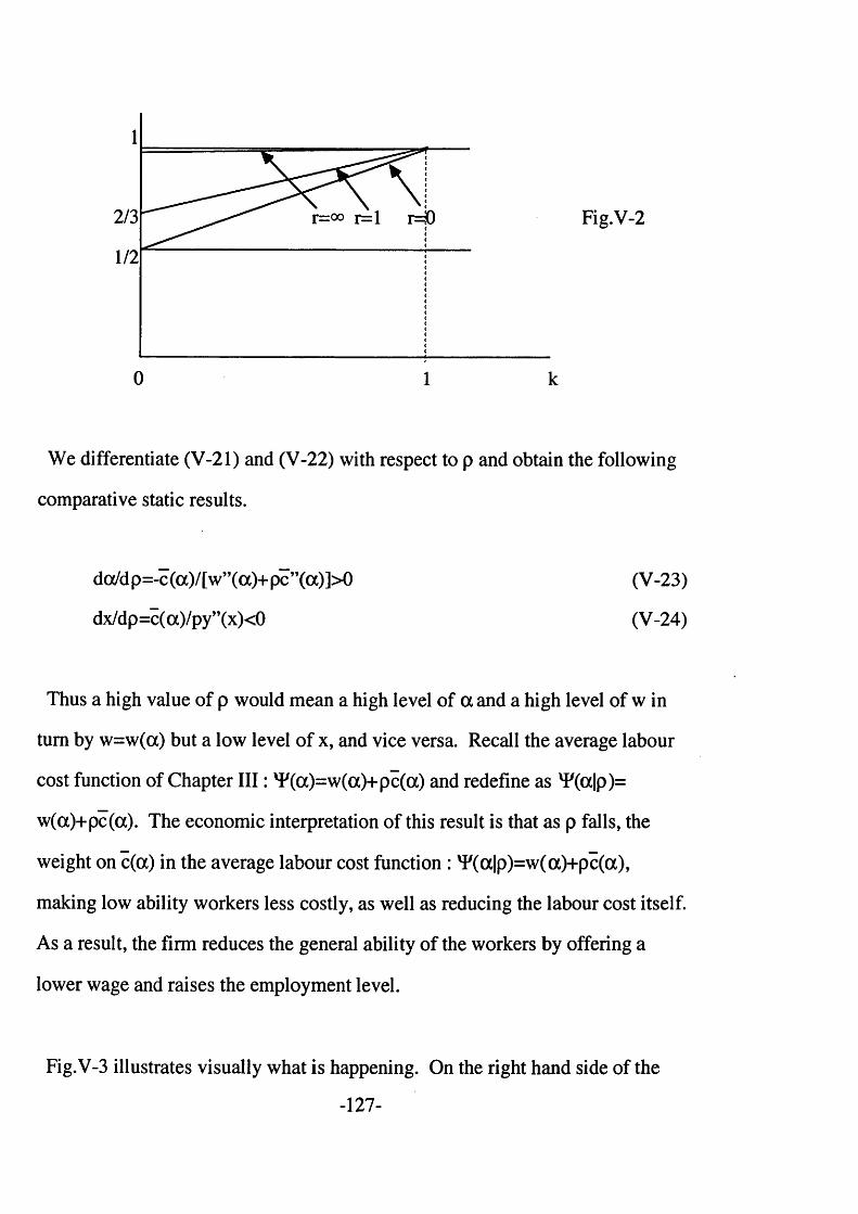
1
2/3 l*=rOO r=l HO
1/2
Fig.V-2
0
We differentiate (V-21) and (V-22) with respect to p and obtain the following
comparative static results.
da/dp=-c(a)/[w”(a)+pc”(a)]>0 (V-23)
dx/dp=c(cc)/py”(x)<0 (V-24)
Thus a high value of p would mean a high level of a and a high level of w in
turn by w=w(a) but a low level of x, and vice versa. Recall the average labour
cost function of Chapter I I I : vF(a)=w(oc)+pc(a) and redefine as 'F(a|p)=
w(a)+pc(a). The economic interpretation of this result is that as p falls, the
weight on c(a) in the average labour cost function : xF(a|p)=w(a)+pc(a),
making low ability workers less costly, as well as reducing the labour cost itself.
As a result, the firm reduces the general ability of the workers by offering a
lower wage and raises the employment level.
Fig.V-3 illustrates visually what is happening. On the right hand side of the
-127-
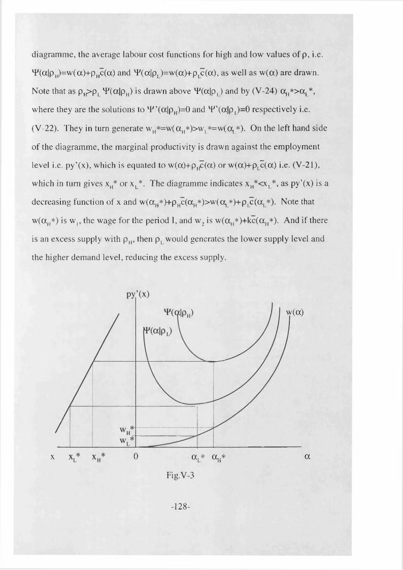
diagramme, the average labour cost functions for high and low values o f p, i.e.
4/ (a |p H)= w (a)+ p Hc(a) and T/(a |p L)=w(oc)+pLc(a), as well as w (a ) are drawn.
Note that as p H> p l ^ (a lp ^ is drawn above ^ (a lp ,) and by (V-24) (^*>0^*,
where they are the solutions to ^ ’(c lpH)=0 and vF’(o lpL)=0 respectively i.e.
(V-22). They in turn generate w H*= w (aH*)>wL*=w((XL*). On the left hand side
o f the diagramme, the marginal productivity is drawn against the employment
level i.e. py’(x), which is equated to wCcO+p^cCa) or w (a)+ p Lc(a ) i.e. (V-21),
which in turn gives xH* or x L*. The diagramme indicates x H*<xL*, as py’(x) is a
decreasing function of x and w (a H*)+pHc(otH*)>w(o(L*)+pLc (a L*). Note that
w (a H*) is w ,, the wage for the period I, and w 2 is w(otH*)+kc(cxH*). And if there
is an excess supply with pH, then pL would generates the lower supply level and
the higher demand level, reducing the excess supply.
w (a)
0 ocL* <V ax
Fig.V-3
- 128 -
Let us verify this result in terms of r, the discount rate and k, the parameter of
general applicability of the training. Firstly, the higher the discount rate is the
closer p becomes to one and the more it resembles to the one-period case. This
is not surprising since a high discount rate means less importance attached to
the future activities. Because the training cost incurs in the period I and the
benefit of training is generated in the period II, the firm would put more on
reducing the cost than when the discount rate is high i.e. r is large. To see this
consider (V-20) when r=0 and r— i.e. 2{py(x)-[w(a)+(l/2)(l+k)c(oc)]x} and
py(x)-[w(a)+c(a)]x respectively. The coefficient c(a) is larger relative to the
coefficients of w(a) in the latter case. As a result the firm would quote a higher
wage to attract workers with lower training cost i.e. abler workers, and the
employment level will be lower because of the higher labour cost. As for the
market equilibrium, an increase in the supply of labour as a result of the wage
increase and a decrease in the demand for labour as a result of the labour cost
increase will make the excess supply more likely, as long as the supply condi
tions remains unchanged.
Secondly, a large value of k has essentially the same effect on the firm’s
behaviour as well as on the labour market equilibrium as that of r through p.
Consider two types of training with one being more specific than the other and
call them specific training and general training with parameters ks<kg respective
ly. By the analogous argument to those of pH>pL, the optimal wages will be
such that ws*=w(as*)<wg*=w(ocg*) since a s*<ag*. Thus the period I wage is
higher for the job offering general training than specific training. In order to see
-129-

the way the generality of training affects the period I wage, rewrite (V-20) as
PV(tu)={ 1+(1 +r)-‘ }{py(x)-[w( a)+( 1 +r+k)(2+k) ',c(a)]x} (V-20) ’
The more general the training is, the higher k and thus the opportunity wage
will be. This makes the coefficient on c(a) larger and the optimal wage will be
larger, as an increase in a reduces the training cost term (l+r+k)(2 +k)'lc(a)
more than it raises the wage cost term w(a) with higher k. Note that the de
mand for labour i.e. x, will be lower for the general training as high k means
generally high labour cost w(a)+(l+r+k)(2+k)‘1c(a). This together with larger
labour supply due to a higher wage offer means that the excess supply is more
likely for general training at the equilibrium. ( See Fig.V-3)
The wage profiles will be {w(as*), w (as*)+ksc(as*)} for the specific training
and {w(ag*), w (ag*)+ kgc(ag*)} for the general training, where
w(as*)+ksc(as*)< w (ag*)+kgc(ag*) can be shown with some extra calculations.
We need to determine the sign of
(d/dk)[w(a)+kc(a)] given w ’(oc)+(l+r+k)/(2 +r)c’(cx)= 0
Now (d/dk)[w(a)+kc(a)]=[w’(oc)+kc,(oc)](da/dk)+c(a)
But w’(a)+pc’(oc)=0 implies w ,(oc)+(k-k+p)c’(oc)=0. Thus,
-130-

w,(ot)+kc’(oc)=(k-p)c,(oc)=[(l+r)(k-l)/(2 +r)]c,(oc)> 0
since k<l & c’(oc)<0. And differentiating w’(cc)+(l+r+k)/(2+r)c’(cc)=0 with
respect to k, we obtain,
w”(oc)(da/dk)+(2 +r) A c ,(a)+[(l+r+k)/(2 + r)]?’(a)(da/dk )= 0
da/dk=- c’(oc)/(2 +r){w”(oc)+[(l+r+k)/(2 +r)]c”(oc)} > 0
since c’(oc)<0 & w”(oc)+[(l+r+k)/(2+r)]c”(oc)>0. Thus
(d/dk) [w(a)+kc(a)]=[w ’ (ot)+kc’(oc)](d a/dk)+c(a)> 0
Therefore if ks<kg, w (as*)+ksc(as*)< w (ag*)+kgc(ag*) i.e. the more general the
training is, the higher the wage profile will be. Furthermore, as k increases
from 0 to 1 , the difference between the wages of the two periods i.e. kc(a)
increases from 0 to c(a). Thus the wage profile becomes steeper with the
generality of training between the two polar cases. ( The rate of wage increase
from the period I to the period II can be defined by kc(a)/w(a). And widening
of the difference by the generality of training would mean d/dk{kc(oc)/w(oc)}>0 .
However, without specifying the functional forms of c(a) and w(a), this sign is
indeterminate for 0<k<l.) On the other hand, the demand for labour is higher
for the specific training i.e. xs*>xg*, while each firm receives less workers for
the specific training case as ws*<wg*. Then the excess supply in the labour
market will be reduced and the possibility of market clearing will emerge.
-131-

These results are summarized in Table V-l and Fig.V-4
The last result does not seem convincing at the first glance. One may expect
that relatively general training creates a fairly competitive atmosphere, as the
acquired skill itself is applicable in all the firms. However, what really happens
here is that a higher opportunity wage in the period II raises the average labour
cost over the two periods and as a result the labour demand is reduced. At the
same time the increased weight on the training cost i.e. kc(a) raises the optimal
wage and that attracts more workers. Together, they are more likely to generate
an excess supply equilibrium than with relatively specific training in the labour
market.
Type of training
k
Optimal wage
Wage profile: w,
:w 2
Labour demand
Market equilibrium is more likely to be;
More specific
K
ws*=w(as*)
w (a * )
w (as*)+ksc (a s*)
xs*
Market clearing
Table V-l
More general
< k 8
< wg*=w (ag*)
< w (a g*)
< w (ag*)+kgc(ag*)
> VExcess supply
-132-

w (a g*)+c(ag* ) : kg=l
w (a g*)
w(oc*)
w (a*)
w (a*)+kc(a*): 0 <k<l
w (a *): k = 0
Period I Period II
Fig.V-4 : The wage profile
In this chapter we have established the following;
Firstly, a two-period training model of heterogeneous labour was introduced
and contrasted with the adverse selection model of Weiss (1980) as well as the
training models such as Donaldson & Eaton (1976), Nickell (1976), and Ohashi
(1983). The model presented in this Chapter has several unique features com
pared with these models. For example, it can be more easily extended to a
multi-period case than the Weiss model, in which an upward-sloping wage
profile can be derived. But unlike most of the training models the introduction
of heterogeneity of labour in terms of training cost means that the firm initially
pays for the training whether it is general or specific, although, as in the stan
dard theory of tax incidence, the actual incidence would depend on the elastic
ities of supply of and demand for labour. The training type instead affects the
alternative wage of the period II.
-133-
Secondly, the firm maximized the profit for each period. It turned out that the
firm’s first order conditions were identical in the two periods. They were also
equivalent to those of Chapter III except that the period II wage was higher due
to the higher alternative wage.
Finally, we assumed that the firm maximized the present value of the profit
stream. With no turnover an upward-sloping wage profile was derived. The
firm’s decision and the consequent market equilibrium depended in particular
on the generality of training. On the whole, the more general the training is, the
higher the wage profile will be, the lower the employment level will be, and the
more likely that the equilibrium entails the excess supply.
-134-

CHAPTER V I : MONOPSONY AND COMPETITION IN
HETEROGENEOUS LABOUR MARKETS
We have established earlier on in Chapter III that in a heterogeneous labour
market, where workers differ in the training costs, a competitive equilibrium
does not always imply market clearing unlike in the case of a homogeneous
labour market. One might, then, wonder whether there are similar irregularities
when the heterogeneous labour market is not competitive.
Consider monopsony, as a typical form of non-competitiveness in labour
markets. It will be shown that the set of profit maximizing conditions of a
monopsony firm is identical to that of a competitive firm in certain cases. The
rationale behind this result is that if the supply of labour is not binding in the
competitive equilibrium, i.e. if there is an excess supply, then this information
about the supply , which a monopsony firm has an access to, becomes redun
dant.
Consider a heterogeneous labour market of the type described in the earlier
chapter, where the workers are heterogeneous in a and consequently in w(a),
the acceptance wage and in c(a), the cost of OJT. As the difference between
competitive equilibrium and monopsony in a labour market lies in the availabili
ty of information on the supply of labour to the firm/firms, we may illustrate
this formally by using the Lagrangian method, for which the supply information
-135-

acts as a constraint. We also extend the Lagrangian method to analyse within
the same framework the homogeneous case, in which there is a well-established
result that monopsony always produces lower levels of wage and employment
than competitive equilibrium.
(1) The Lagrangian and the Constraint
Define the profit equation in the following form.
tv= py(xd)-wxd-Cxd (VI-1)
This is identical to (III-6 ) of Chapter III except that w and C are not the func
tions of a . And we introduce constraints, with X's being the multipliers, as
(i) ^,:w=w(a)
(ii) ^ 2:C=c(a)
(iii) ^ 3:w>Ws(xd)
so that the Lagrangian is given by
L=py(xd)-(w+C)xd+X1((w-w(a))+A,2(C-c(a))+A,3(w-Ws(xd)) (VI-2)
(i) and (ii) express the heterogeneity of the labour force through the reservation
wage and the average cost of OJT, both of which vary with a . Note that (VI-1)
with these constraints is (III-6 ), i.e. 7t= py(xd)-c(Gc)xd-w(a)xd, or it is identical to
optimize (VI-2) with being restricted to zero. In the following discussion we
-136-
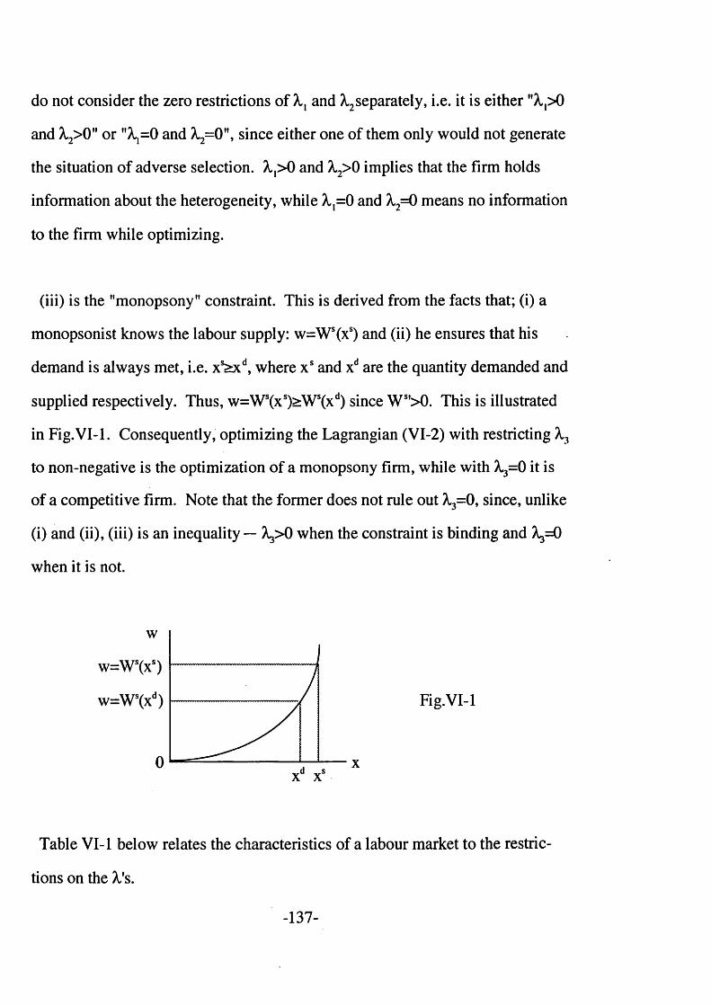
do not consider the zero restrictions of X { and ^separately, i.e. it is either "A,,> 0
and X.2>0 " or " ^ = 0 and ^ 2=0 ", since either one of them only would not generate
the situation of adverse selection. A, ,> 0 and A,2> 0 implies that the firm holds
information about the heterogeneity, while A, ,= 0 and A,2= 0 means no information
to the firm while optimizing.
(iii) is the "monopsony" constraint. This is derived from the facts that; (i) a
monopsonist knows the labour supply: w=Ws(xs) and (ii) he ensures that his
demand is always met, i.e. x*>xd, where x s and xd are the quantity demanded and
supplied respectively. Thus, w=Ws(xs)>Ws(xd) since W s,>0. This is illustrated
in Fig.VI-1. Consequently, optimizing the Lagrangian (VI-2) with restricting
to non-negative is the optimization of a monopsony firm, while with ^ = 0 it is
of a competitive firm. Note that the former does not rule out X,3=0, since, unlike
(i) and (ii), (iii) is an inequality — ^ > 0 when the constraint is binding and ^ = 0
when it is not.
w
w=Ws(xs)
w=Ws(xd) Fig.VI-1
0 x
Table VI-1 below relates the characteristics of a labour market to the restric
tions on the X's.
-137-
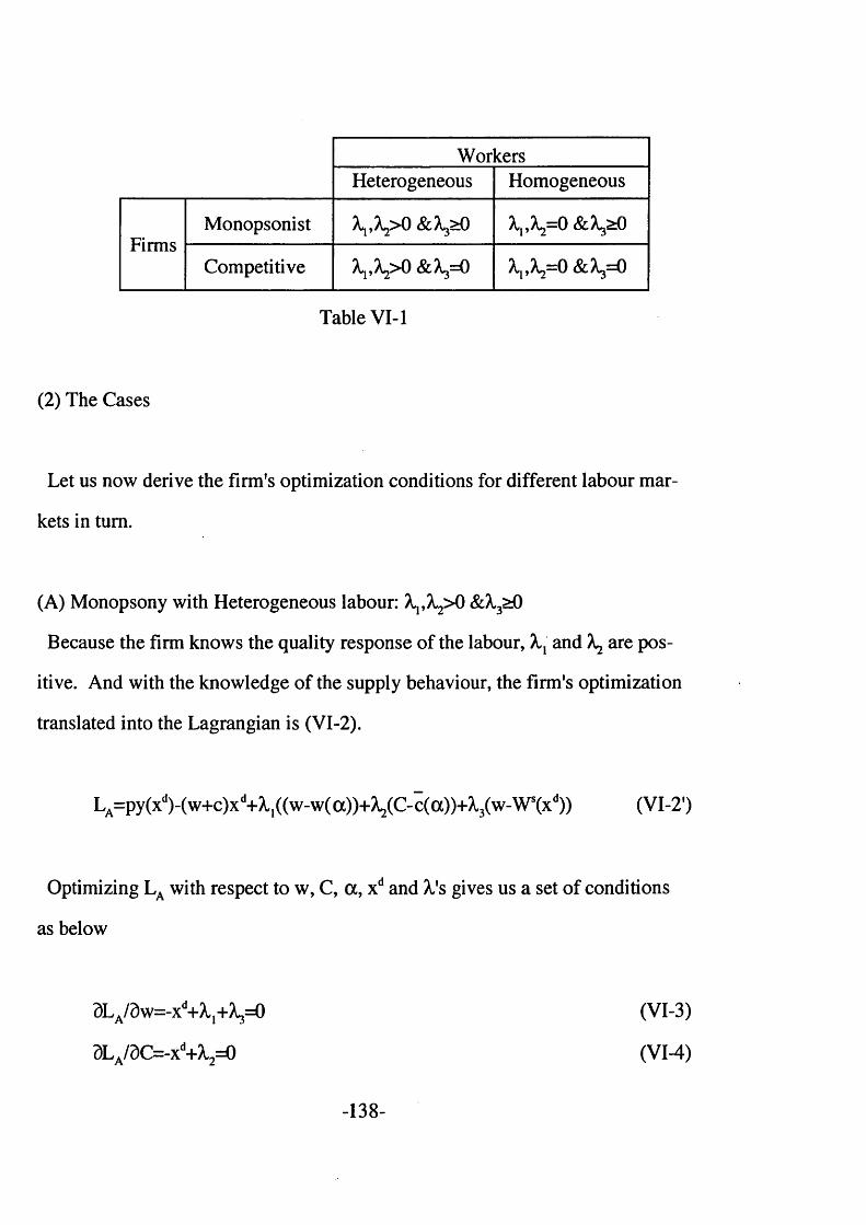
Wor cersHeterogeneous Homogeneous
FirmsMonopsonist A,j,A2>0 ^ ,^ = 0 & ^>0
Competitive Xp \ > 0 & x = $ ^ ,^ = 0
Table VI-1
(2) The Cases
Let us now derive the firm's optimization conditions for different labour mar
kets in turn.
(A) Monopsony with Heterogeneous labour: X-pX2>0 &X,3>0
Because the firm knows the quality response of the labour, and 7 are pos
itive. And with the knowledge of the supply behaviour, the firm's optimization
translated into the Lagrangian is (VI-2).
LA=py(xd)-(w+c)xd+A,1((w-w(a))+A2(C-c(a))+^3(w-Ws(xd)) (VI-2')
Optimizing LA with respect to w, C, a , xd and X's gives us a set of conditions
as below
dL^Sw^x^A.j+AysO
dLA/dC=-xd+A,2=0
(VI-3)
(VI-4)
dLA/da^-A y(a)-A ,2c '(a )= 0 (VI-5)
^/dx^pyX x^-C w +cJ-^W 'C x^O (VI-6 )
dLA/dA,,=w-w( oc)=0 (VI-7)
dl^/dA^C-ctcc^O (VI-8 )
3LA/dX3=w-Ws(xd)=0 (VI-9)
From (VI-3) (VI-4) and (VI-5), from (VI-6 ) (VI-7) and (VI-8 ) and from (VI-
7) and (VI-9) respectively,
(xd-X,3)w'(a)+xdc,(oc)=0 (VI-10)
py’(xd)=w(a)+c(a)+X3W s,(xd) (VI-11)
w(a)=Ws(xd) (VI-12)
From (VI-10) and (VI-11), by eliminating A3, we obtain,
py’(xd)=w(a)+c(a)+(xd/wf(a))(w '(a)+c,(a))W s'(xd) (VI-13)
This is consistent with the usual monopsony condition in a labour market that
at the equilibrium marginal productivity of labour (i.e. LHS of (VI-13)) is
equated to marginal cost of labour (i.e. RHS of (VI-13)), since the marginal cost
of labour is,
d/dxd(total cost)=d/dxd{(w(a)+c(a))xd}
=w(a)+c(a)+x d{ w'(oc)+c'( cx)}(da/dxd)
-139-

=w(a)+ c(a)+xd{ w'(oc)+c'( a)}(Ws,(xd)/w'( a))
where, from totally differentiating (VI-12), w’(oc)da=Ws,(xd)dxd
(B) Competitive market with Heterogeneous labour: A,j,A,2>0 &^3=0
As the firm does not know the supply response of the workers, it maximizes
profit in the absence of constraint (iii). Thus the Lagrangian is,
LB=py(xd)-(w+C)xd+X,1((w-w(a))+X2(C-c(a)) (VI-14)
and this is optimized with respect to w, C, a , xd, and so that we obtain
dLB/dw=-xd+A,,=0 (VI-15)
d L B/d C = -x d+X2=0 (VI-16)
d L g /S a ^ ^ w X ^ -^ c ^ a )^ (VI-17)
dLB/dxd=pyf(xd)-(w+C)=0 (VI-18)
dLB/dA,=w-w(oc)=0 (VI-19)
d h B/dX2= C -c ( a)=0 (VI-20)
From (VI-15) (VI-16) and (VI-17), and from (VI-18) (VI-19) and (VI-20)
respectively,
w’(a)+c'(cx)=0 (VI-21)
py'(xd)=w(a)+c(a) (VI-22)
-140-
which are the optimization conditions derived in Chapter III for a competitive
firm, i.e. (III-8 ) and (III-7) respectively. In order to make comparable the
market demand in monopsony and competitive equilibrium, we let xd be the
market demand by letting n= l, where n is the number of firms. Note that we do
not lose generality by doing so, as we assume the lack of information to mean
the competitiveness.
The optimization conditions (VI-10) (VI-11) and (VI-12) of monopsony would
be equivalent to those of a competitive firm i.e. (VI-21) and (VI-22) if X3=0,
since, with ^= 0 , (VI-12) disappears. Furthermore, when X,3=0 holds for monop
sony, competitive equilibrium exhibits an excess supply of labour since the
equilibrium conditions for monopsony are those of competitive equilibrium i.e.
w'(oc)+cf(oc)= 0
py' (xd)=w(a)+c (a)
w(a)>Ws(xd)
It needs to be pointed out that in the case A, i.e. the case of monopsony with
heterogeneous labour, the possibility of 3= 0 can not be ruled out a priori — it
will be shown later that in the case of monopsony with homogeneous labour
^3= 0 holds only at zero production. For, from (VI-3), X,3=xd-^ 1, and ^ > 0 by
assumption so that is non-negative rather than strictly positive. Therefore,
when a competitive equilibrium is characterized by an excess supply or equally
-141-

non-binding labour supply, it is indistinguishable from monopsony. Whether
^ = 0 holds or not depends on the exogeneously given functions y(#), w(*), c(*)
and h(*) and product price p in a similar manner to the one described earlier in
determining whether an excess supply exists with competitive equilibrium.
When X3>0, on the other hand, the supply condition is binding and from (VI-
10),
w'(a)+c'( a)=( Xi/x d)wX a)>0 (VI-1 O')
which means that the equilibrium wage is above the optimum wage. In this
case, competitive equilibrium exhibits market clearing i.e. the labour supply is
binding, since ^ > 0 means that the profit a competitive firm would be increased
if the supply information was available. Therefore, when X3> 0 , monopsony and
competitive equilibrium are distinct and both are characterized by the binding
labour supply.
Fig.VI-2 shows the comparison of the two equilibria for different values of Xy
Note in particular that X,3=0 holds as long as competitive equilibrium (CE) is
characterized by an excess supply of labour, where the two equilibria are identi
cal (See Fig.VI-2(a) and (b)). But once competitive equilibrium exhibits market
clearing, the two equilibria become distinct with monopsony (M) offering lower
levels of wage and employment than competitive equilibrium (See Fig.VI-2(c)).
-142-

CDF MC
S=AC
CE
x
CDFw
CE=
0 x
CDFw
CE=
0
Fig. VI-2
(C) Monopsony with Homogeneous labour: A,j=0 and ^= 0 &X3>0
In maximizing the profit, the firm knows the supply of labour i.e. X3>0. How
ever, for the moment we allow X to be non-negative. Then the Lagrangian is
Lc= py(xd)-(w+C)xd+X3(w-Ws(xd)) (VI-23)
Optimizing with respect to w, xd and X3, we obtain
d L J d w = - x d+ \ = 0 (VI-24)
dLc/dxd=py,(xd)-(w+C)-X3Ws,(xd)=0 (VI-25)
(VI-26)
It can be seen from (VI-24) that X3 is zero only when xd is zero — in other
words, when production takes place the firm always makes use of the supply
-143-
information, unlike in the heterogeneous case we have just discussed. Elim
inating X3 from (VI-25) and (VI-26), we obtain the usual monopsonist’s equilibri
um condition
py'(Xd)=(w+C)+XdWs,(xd) (VI-27)
This is the optimization condition in monopsony that marginal productivity of
labour is equated to marginal cost of labour.
(D) Competitive market:A,,=0 and A,2=0 &X,3=0
The firm has to maximize the profit with w as given so ^3=0 . Thus the
Lagrangian is
Note that the optimization condition of monopsony (VI-25) would be equiv
alent to that of a competitive firm (VI-28) if X,3=0, analogous to the heter
ogeneous cases described earlier. However, in the homogeneous case ^ 3=0
implies no production by (VI-24). Hence competitive equilibrium and monopso
ny are always distinct as long as there is production.
LD=py(xd)-(w+C)xd (VI-28)
Optimizing with respect to xd will give us a condition
py'(xd)=w+C (VI-29)
-144-

In this chapter we have established that in a heterogeneous labour market an
equilibrium in monopsony and competitive equilibrium are not necessarily
distinct states as is the case in a homogeneous labour market. Using the
Lagrangian approach, they are shown to be indistinguishable when the compet
itive equilibrium is characterized by an excess supply of labour. This is the case
where w=Ws(x) is not binding. And they are distinct as in the homogeneous
case when competitive equilibrium is characterized by market clearing. Wheth
er this occurs, of course, depends on the relative natures of the functions y(*),
w(*), c(*) and h(*) and the level of product price.
-145-

CHAPTER V I I : COMPARATIVE STATICS
We have so far argued that the nature of a competitive equilibrium of a heter
ogeneous labour market depends on the behaviour of the following functions;
production function :y(*), opportunity wage function :w(*), training cost func
tion :c(«) and distribution function of ability :h(«), as well as on the level of
product price, p. Together they determine whether the equilibrium is character
ized by market clearing or an excess supply of labour through the supply of and
demand for labour. This can be seen by recalling how they were defined in
Chapter III. The supply was defined by;
a(w) is an inverse function of w(a).
On the other hand, the demand of each firm was derived in Chapter III from a
set of conditions; the conditional demand function (CDF) and the optimal wage
function (OWF);
SL: Ns(w)=mxs(w)=nH(a(w)) (III-15)
where Ns is the aggregate labour supply
m is the number of firms
xs is the labour supply that each firm faces
-146-

CDF:0(xd,w)=(|) i.e. w=py’(xd)-c(oc(w))
OWF:vi/ '(a)=w'(a)+c'(a)=0 (VII-2)
(VIM )
And for the market as a whole, (VII-1) may be written in terms of Nd, so that
Thus from (111-15) (VIM ') and (VII-2), we see that;
(i) a shift in y(*) affects CDF only.
(ii) a shift in w(*) affects the supply, CDF and OWF.
(iii) a shift in c(*) affects CDF and OWF.
(iv) a shift in h(*) affects the supply, CDF and OWF.
(v) a change in p affects CDF only.
In this chapter before considering the precise effects of these functions and the
price levels on the equilibrium levels of wage and employment, let us describe
the effects of these on the demand and the supply sides of the market separately.
(1) The functions
(a) Production function : y(»)
We assume y(*) to be identical to all firms since for each production process
its particular characteristics is assumed to be expressed by c(#).
CDF:0(Nd,w)=(t) i.e. w=py'(Nd/m)-c(a(w))
OWF:vF'(a)=w'(a)+c'(a)=0
(VII-1')
(VII-2)
-147-
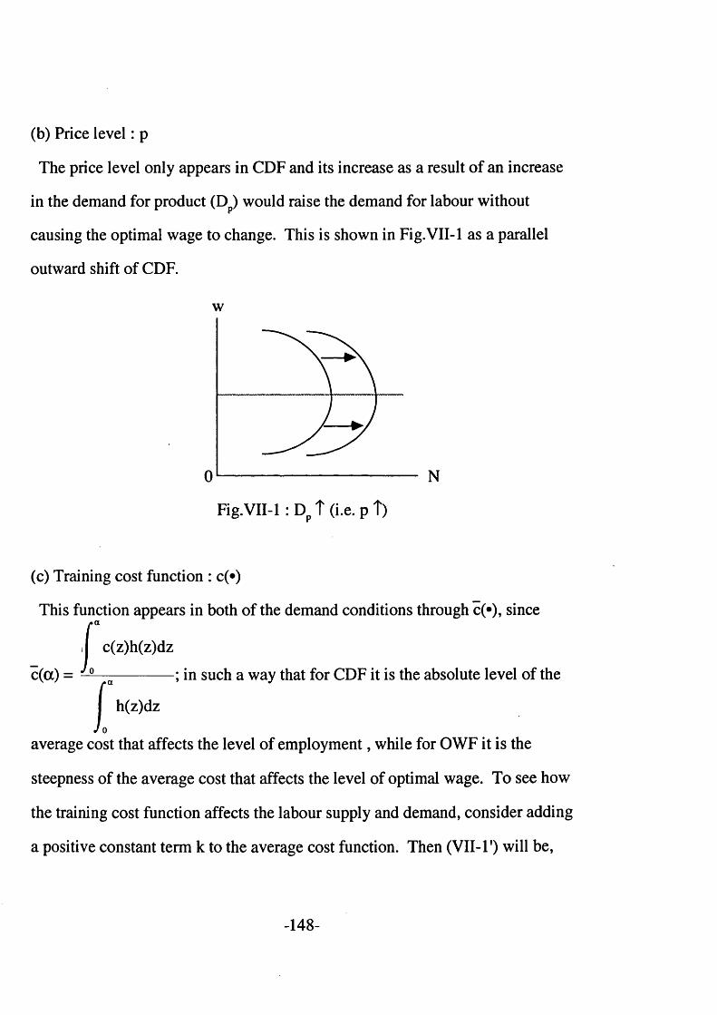
(b) Price level: p
The price level only appears in CDF and its increase as a result of an increase
in the demand for product (Dp) would raise the demand for labour without
causing the optimal wage to change. This is shown in Fig.VII-1 as a parallel
outward shift of CDF.
w
0
Fig.VII-1: Dp T (i.e. p T)
(c) Training cost function : c(»)
This function appears in both of the demand conditions through c(«), sincer11 c(z)h(z)dz
c(a) = -------------; in such a way that for CDF it is the absolute level of the
I h(z)dz J 0
average cost that affects the level of employment, while for OWF it is the
steepness of the average cost that affects the level of optimal wage. To see how
the training cost function affects the labour supply and demand, consider adding
a positive constant term k to the average cost function. Then (VII-1') will be,
-148-

w=py’(Nd/m)-c(a(w))-k (VII-1")
This means a general increase in labour cost, which results in the reduction of
the labour demand. Note that this does not affect the optimal wage since the
optimal wage is solely determined by OWF. (See Fig.VII-2(a)) Now suppose
c(a) is replaced by kc(a) where k> l. The new OWF will be,
w'(a)+kc'(oc)=0 (VII-2')
or w'(a)+c'( a)=( 1 -k) c'(a)>0
Thus at the ability level that satisfies (VII-2') the original OWF is positive.
Because both w(«)+c(*) and w(*)+kc(*) have a single local minimum, a steeper
c(#) implies an increased optimum value of a and thus of w. On the other hand,
how this affects the optimal quantity is indeterminate since the change of the
slope can not be separately analysed from the change of the absolute level of
c(*). This is illustrated as an upward shift of the original OWF in Fig.VII-2(b).
We still need to see how c(*) and c(«) are related. Suppose c(*) is increased by
k, then
/ * a
(c(z)+k)h(z)dz
= c(a)+k (VII-3)• a
h(z)dz0
-149-

implying that c(a) will equally be increased by k. Now suppose c(*) is in
creased to kc(*) s.t. k>l, i.e. c(*) is steeper for all values of a , then
kc(z)h(z)dz
0 = kc(a)
h(z)dz
(VIM)
implying that c(a) will also be steeper by k. Thus (i) a generally high valued
c(*) generates lower labour demand and thus the demand function i.e. CDF
nearer to the vertical axis and (ii) a steeper c(«) implies a higher optimal wage,
which means the demand function away from the horizontal axis.
w w
0
(a) a high valued c(a)
N 0 N
(b) a steeper c(a)
Fig. VII-2
(d) Distribution of ability : h(a)
If a is the sole and innate ability of each individual worker, then this distribu
tion is exogeneous to the model. There are at least three cases in which a
-150-

change of h(a) may be taken into consideration. Firstly, a may be an observ
able part of the innate ability, in which case a different type of observation or
screening could generate a different distribution, d((3) say. Secondly, a may be
achieved through educational investment, in which case more education would
mean that the distribution is more concentrated at higher values of a . The
government may be interested in such a policy to raise the general standard of
education. Thirdly, a demographic change could cause the distribution to
change its shape. For example, immigration of workers with relatively high a
into the country or emigration of workers with relatively low a from the country
would again generate h(a) with relatively high density at higher values of a .
Here, consider what will happen to the supply and demand conditions when
the distribution h(a) becomes high density at higher values of a , as a result of
the government policy to raise the educational level of the population or to
allow in the immigration of workers with relatively high level of ability. Note
that a difficulty arises when the effect of a change in h(a) is discussed, since
this function appears in all of the three conditions of the supply and demand.
The supply response to a change in the distribution h(*) differs between (i)
when the quality of the existing population improves and (ii) when extra supply
of the high quality workers is added. In (i) as the total quantity is unchanged,
there will be equal or less number of workers willing to work than before at all
wage and this causes the supply to shift to left. In (ii) the high quality workers
from outside are added to the domestic supply at the corresponding wage levels
and this causes the supply to shift to right. This is shown in Fig.VII-3(a).
-151-
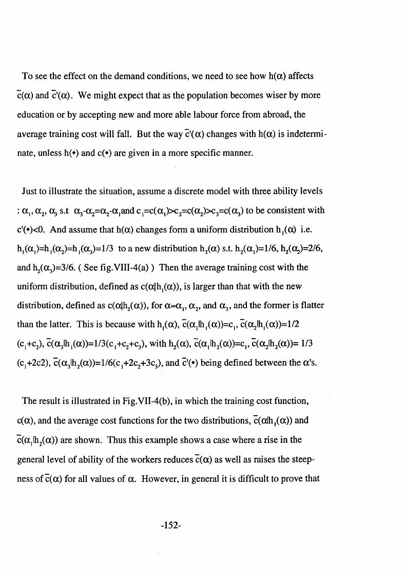
To see the effect on the demand conditions, we need to see how h(a) affects
c(a) and c'(oc). We might expect that as the population becomes wiser by more
education or by accepting new and more able labour force from abroad, the
average training cost will fall. But the way c'(oc) changes with h(a) is indetermi
nate, unless h(*) and c(*) are given in a more specific manner.
Just to illustrate the situation, assume a discrete model with three ability levels
: a ,, a 2,0Cj s.t a 3-a2= a 2-a,and Cj=c(a,)>c2=c(a2)>c3=c(a3) to be consistent with
c'(*)<0. And assume that h(a) changes form a uniform distribution h,(a) i.e.
h ,(a1)=hl(a 2)=hI(a 3)=l/3 to a new distribution h2(a) s.t. h2(a,)= l/6 , h2(a^)=2l6,
and h2( a 3)=3/6. ( See fig.VIII-4(a)) Then the average training cost with the
uniform distribution, defined as c(oc|h,(a)), is larger than that with the new
distribution, defined as c(oc|h2(a)), for a = a p a 2, and oc3, and the former is flatter
than the latter. This is because with h,(a), cCcXjIh^a))^,, c (a2lh,(a))=l/2
(c,+c2), c (a3lh1(a))= l/3(c1+c2+c3), with h2(a), c ta jh ^ a ) ) ^ , , c (a2lh2(a))= 1/3
(c,+2c2), c (a 3lh2(a))= l/6(c1+2c2+3c3), and c'(#) being defined between the a's.
The result is illustrated in Fig.VII-4(b), in which the training cost function,
c(a), and the average cost functions for the two distributions, c(odh,(a)) and
c(ajlh2(a)) are shown. Thus this example shows a case where a rise in the
general level of ability of the workers reduces c(a) as well as raises the steep
ness of c(a) for all values of a . However, in general it is difficult to prove that
-152-
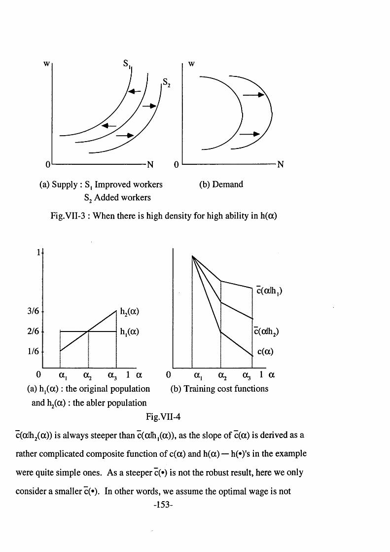
w
0
S2
0
(a) Supply : S, Improved workers (b) DemandS2 Added workers
Fig.VII-3 : When there is high density for high ability in h(a)
c(alh2)
, c(a)
0 a '2
3/6
2/6
1/6
0 a 3 1 aa 2(a) h j( a ) : the original population (b) Training cost functions
and h ^ a ) : the abler population
Fig.VII-4
c(alh2(a)) is always steeper than c(alh,(a)), as the slope of c(a) is derived as a
rather complicated composite function of c(a) and h(a) — h(*)’s in the example
were quite simple ones. As a steeper c(») is not the robust result, here we only
consider a smaller c(*). In other words, we assume the optimal wage is not-153-

affected by the change of h(*). This is illustrated in Fig.VII-3(b) by a parallel
outward shift.
(d) Opportunity wage function : w(a)
This function also appears in all of the supply and demand conditions. If
productivity in the alternative job changes, there will be a shift in w(a). For
example, as in Weiss (1980) if the alternative job exhibits diminishing returns
to scale then a reduction in the employment level in the market in question will
in turn induce a fall in the productivity in the alternative sector and hence w(a)
will shift down. This will shift the supply to the right. At the same time this
change in w(a), i.e. jower and flatter w(a) causes a shift in the demand condi
tion in a way similar to that of c(a). ( See Fig.VII-5 ) Under constant returns
to scale, on the other hand, w(a) will be unaltered by the employment level in
the alternative sector. In this model we assume constant returns to scale so that
neither supply nor demand would shifts by a change in the opportunity wage,
w w
0 N 0 N
(a) Supply (b) Demand
Fig.VII-5 : When w(a) shifts downwards
-154-
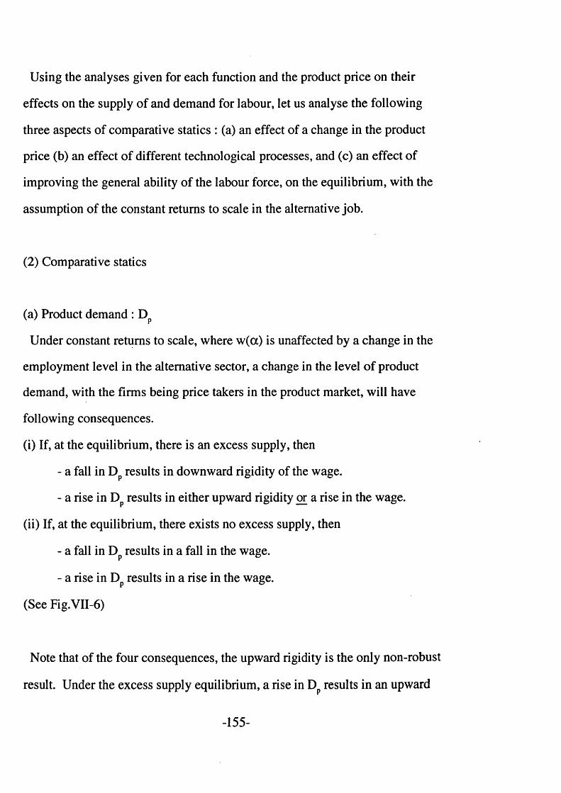
Using the analyses given for each function and the product price on their
effects on the supply of and demand for labour, let us analyse the following
three aspects of comparative statics : (a) an effect of a change in the product
price (b) an effect of different technological processes, and (c) an effect of
improving the general ability of the labour force, on the equilibrium, with the
assumption of the constant returns to scale in the alternative job.
(2) Comparative statics
(a) Product demand : Dp
Under constant returns to scale, where w(a) is unaffected by a change in the
employment level in the alternative sector, a change in the level of product
demand, with the firms being price takers in the product market, will have
following consequences.
(i) If, at the equilibrium, there is an excess supply, then
- a fall in Dp results in downward rigidity of the wage.
- a rise in Dp results in either upward rigidity or a rise in the wage.
(ii) If, at the equilibrium, there exists no excess supply, then
- a fall in Dp results in a fall in the wage.
- a rise in Dp results in a rise in the wage.
(See Fig.VII-6)
Note that of the four consequences, the upward rigidity is the only non-robust
result. Under the excess supply equilibrium, a rise in Dp results in an upward
-155-
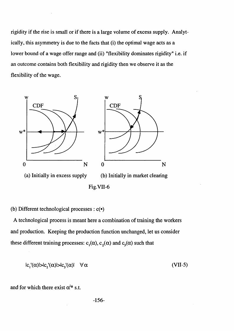
rigidity if the rise is small or if there is a large volume of excess supply. Analyt
ically, this asymmetry is due to the facts that (i) the optimal wage acts as a
lower bound of a wage offer range and (ii) "flexibility dominates rigidity" i.e. if
an outcome contains both flexibility and rigidity then we observe it as the
flexibility of the wage.
CDF
w
0 N
CDF
w
0 N
(a) Initially in excess supply (b) Initially in market clearing
Fig.VII-6
(b) Different technological processes : c(*)
A technological process is meant here a combination of training the workers
and production. Keeping the production function unchanged, let us consider
these different training processes: c,(a), c2(a) and c3(a) such that
Ic,,(a)l>lc2'(a)l>lc3'(a)l V a (VII-5)
and for which there exist a'* s.t.
-156-
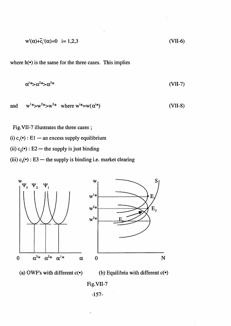
w'CcO+c^oc^O i= 1,2,3 (VII-6)
where h(*) is the same for the three cases. This implies
a 1 *>a2*>a3*
and w'*>w2*>w3* where w'*=w(a'*)
Fig.VII-7 illustrates the three cases ;
(i) c^* ): El — an excess supply equilibrium
(ii) c2(*): E2 — the supply is just binding
(iii) c3(*): E3 — the supply is binding i.e. market clearing
N0a 3* a 2* a 1*0 a
(a) OWF’s with different c(#) (b) Equilibria with different c(#)
Fig.VII-7
-157-
(VII-7)
(VII-8)
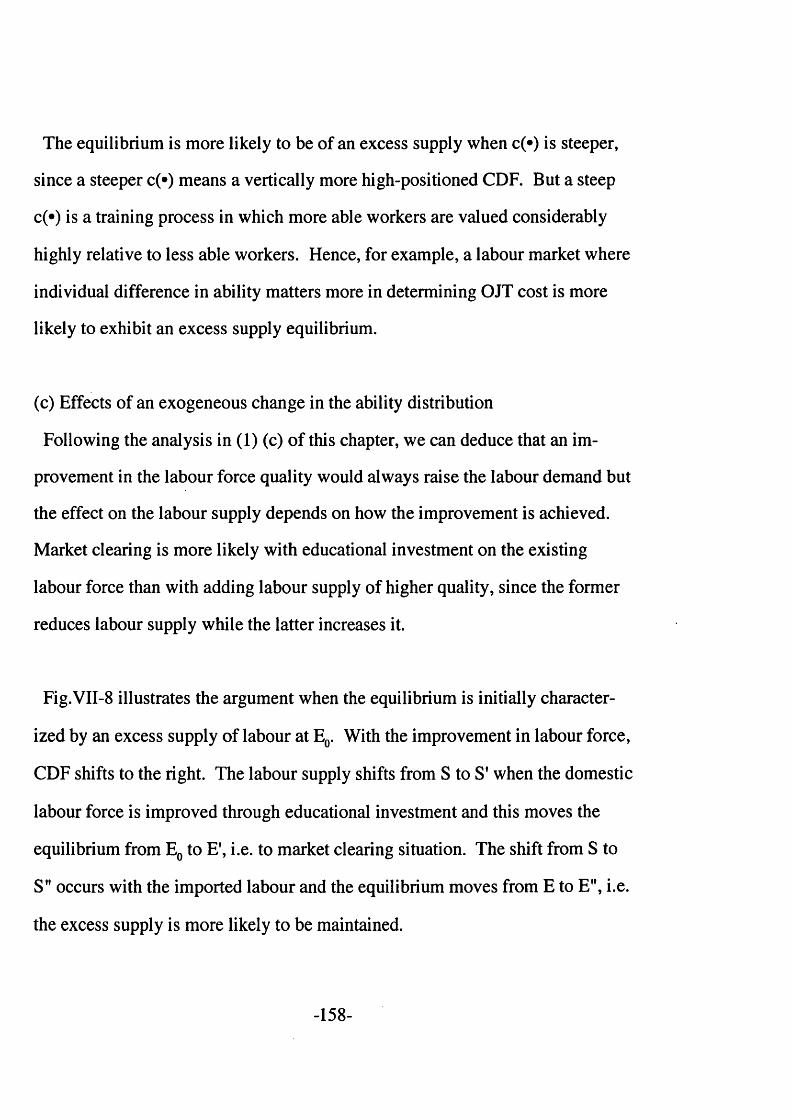
The equilibrium is more likely to be of an excess supply when c(*) is steeper,
since a steeper c(*) means a vertically more high-positioned CDF. But a steep
c(«) is a training process in which more able workers are valued considerably
highly relative to less able workers. Hence, for example, a labour market where
individual difference in ability matters more in determining OJT cost is more
likely to exhibit an excess supply equilibrium.
(c) Effects of an exogeneous change in the ability distribution
Following the analysis in (1) (c) of this chapter, we can deduce that an im
provement in the labour force quality would always raise the labour demand but
the effect on the labour supply depends on how the improvement is achieved.
Market clearing is more likely with educational investment on the existing
labour force than with adding labour supply of higher quality, since the former
reduces labour supply while the latter increases it.
Fig.VII-8 illustrates the argument when the equilibrium is initially character
ized by an excess supply of labour at E0. With the improvement in labour force,
CDF shifts to the right. The labour supply shifts from S to S' when the domestic
labour force is improved through educational investment and this moves the
equilibrium from E0 to E', i.e. to market clearing situation. The shift from S to
S" occurs with the imported labour and the equilibrium moves from E to E", i.e.
the excess supply is more likely to be maintained.
-158-
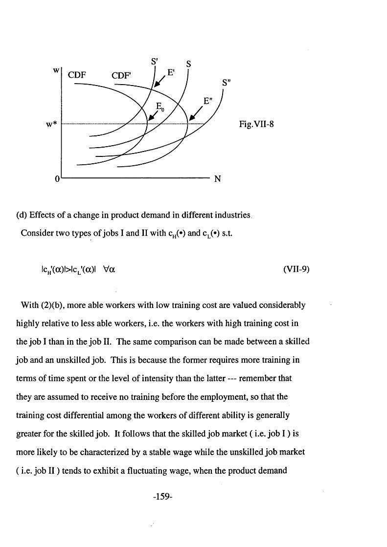
w CDF CDF
w*
0
Fig.VII-8
(d) Effects of a change in product demand in different industries
Consider two types of jobs I and II with cH(*) and cL(*) s.t.
ICnXoOWcjGOI Voc (VII-9)
With (2)(b), more able workers with low training cost are valued considerably
highly relative to less able workers, i.e. the workers with high training cost in
the job I than in the job II. The same comparison can be made between a skilled
job and an unskilled job. This is because the former requires more training in
terms of time spent or the level of intensity than the latter — remember that
they are assumed to receive no training before the employment, so that the
training cost differential among the workers of different ability is generally
greater for the skilled job. It follows that the skilled job market ( i.e. job I ) is
more likely to be characterized by a stable wage while the unskilled job market
( i.e. job I I ) tends to exhibit a fluctuating wage, when the product demand
-159-

changes. Also note the optimal wage i.e. the wage s.t. ^ ’=0 for the skilled job
is higher than for the unskilled job. ( See Fig.VII-9 ) As for the employment
level, this model suggests that the skilled job market tends to have excess sup
ply, while the unskilled job market tends to be in market clearing.
It should be noted here that this result, though it may appear to be contrary, is
compatible with an empirical finding that a skilled labour sector is generally
characterized by a lower level of unemployment. There are two reasons for
this. Firstly, a longer job queue in the skilled sector would imply a higher level
of unemployment in that sector only if the skilled workers are confined to the
skilled labour market. But as various models attempt to show, the skilled
workers are accessible to the unskilled market as well. (See, for example, Fields
(1974) and Bhagwati & Srinivasan (1977)). Under such an assumption the
excess supply figure does not appear as an unemployment figure. Rather the
excess supply becomes an issue of underemployment. This issue is analysed in
the next chapter in the form of heterogeneous firms within one market.
Secondly, a job queue does not necessarily imply unemployment because what
we consider here are "potentially" skilled and unskilled workers. If they had
already been skilled or unskilled by the time they enter the market, they would
have been distinguishable, which does not accord with our assumption. Our
workers are unskilled before the OJT so that if not selected they will still be
unskilled whichever market they apply to.
-160-
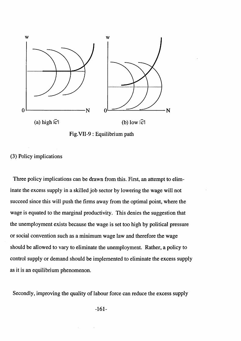
w w
0 N 0 N
(a) high Id (b) low Id
Fig.VII-9: Equilibrium path
(3) Policy implications
Three policy implications can be drawn from this. First, an attempt to elim
inate the excess supply in a skilled job sector by lowering the wage will not
succeed since this will push the firms away from the optimal point, where the
wage is equated to the marginal productivity. This denies the suggestion that
the unemployment exists because the wage is set too high by political pressure
or social convention such as a minimum wage law and therefore the wage
should be allowed to vary to eliminate the unemployment. Rather, a policy to
control supply or demand should be implemented to eliminate the excess supply
as it is an equilibrium phenomenon.
Secondly, improving the quality of labour force can reduce the excess supply
-161-
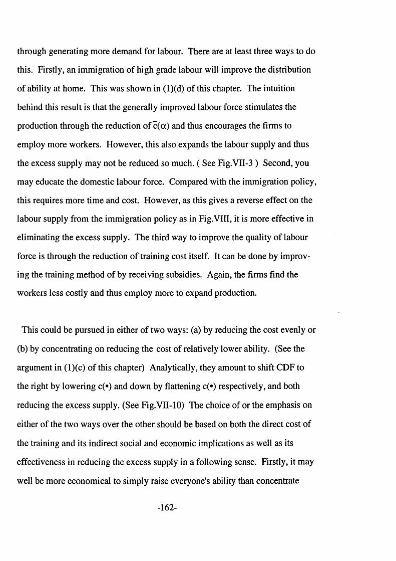
through generating more demand for labour. There are at least three ways to do
this. Firstly, an immigration of high grade labour will improve the distribution
of ability at home. This was shown in (l)(d) of this chapter. The intuition
behind this result is that the generally improved labour force stimulates the
production through the reduction of c(a) and thus encourages the firms to
employ more workers. However, this also expands the labour supply and thus
the excess supply may not be reduced so much. ( See Fig.VII-3 ) Second, you
may educate the domestic labour force. Compared with the immigration policy,
this requires more time and cost. However, as this gives a reverse effect on the
labour supply from the immigration policy as in Fig.VIII, it is more effective in
eliminating the excess supply. The third way to improve the quality of labour
force is through the reduction of training cost itself. It can be done by improv
ing the training method of by receiving subsidies. Again, the firms find the
workers less costly and thus employ more to expand production.
This could be pursued in either of two ways: (a) by reducing the cost evenly or
(b) by concentrating on reducing the cost of relatively lower ability. (See the
argument in (l)(c) of this chapter) Analytically, they amount to shift CDF to
the right by lowering c(*) and down by flattening c(*) respectively, and both
reducing the excess supply. (See Fig.VII-10) The choice of or the emphasis on
either of the two ways over the other should be based on both the direct cost of
the training and its indirect social and economic implications as well as its
effectiveness in reducing the excess supply in a following sense. Firstly, it may
well be more economical to simply raise everyone's ability than concentrate
-162-

CDFCDFCDFw
CDF
NN 0
(a) Lower c(*) (b) Flatter c(*)
Fig.VII-10
on raising the ability of a particular group of workers. Secondly, 'a uniformaliza
tion' of the workers' ability through raising more the ability of the relatively
lower ability workers may act to give equal opportunity to everyone in the
society, but at the expense of the more able group. Thirdly, in a long run it
might contribute more to the economic growth if an effort is made to raise even
further the ability of the more able group. Although these are highly important
issues in educational planning, within the present model they are much outside
of the scope of the present paper.
Thirdly, under the excess supply equilibrium an introduction of a minimum
wage gives a different result from what one usually expects. The standard result
of an effect on a minimum wage based on a two-market analysis —
-163-
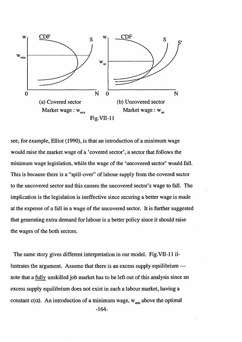
CDF CDFS
min
uc
N0 N 0(a) Covered sector (b) Uncovered sector
Market wage : wmin Market wage : w^Fig. VII-11
see, for example, Elliot (1990), is that an introduction of a minimum wage
would raise the market wage of a ‘covered sector’, a sector that follows the
minimum wage legislation, while the wage of the ‘uncovered sector’ would fall.
This is because there is a “spill-over” of labour supply from the covered sector
to the uncovered sector and this causes the uncovered sector’s wage to fall. The
implication is the legislation is ineffective since securing a better wage is made
at the expense of a fall in a wage of the uncovered sector. It is further suggested
that generating extra demand for labour is a better policy since it should raise
the wages of the both sectors.
The same story gives different interpretation in our model. Fig.VII-11 il
lustrates the argument. Assume that there is an excess supply equilibrium —
note that a fully unskilled job market has to be left out of this analysis since an
excess supply equilibrium does not exist in such a labour market, having a
constant c(a). An introduction of a minimum wage, wmin above the optimal
-164-

wage in the covered sector would initially drive those unemployed to the uncov
ered sector — a shift from S to S’. However, their search of job would be
unsuccessful since the optimal wage in the uncovered sector w^ stays un
changed i.e. the group of workers attracted by the optimal wage still remains the
best choice for the firm. Thus the effect of the legislation is simply to increase
the total excess supply of labour over the two sectors. Hence, while the uncov
ered sector clears with the wage below the minimum wage for the standard
analysis, our model predicts that the wage in the uncovered sector will not be
affected. Also in our model, an increase in the demand for labour may not
result in an immediate increase in the wage as long as an excess supply exists in
that sector. It might be more effective to raise the optimal wage itself. This can
be done by reducing the training cost of relatively able workers, as the firm
would find the able workers less expensive and decide to raise the optimal
wage. Following the argument in (l)(c), one could do so by subsidizing the
training cost of relatively abler workers and thereby reducing their training cost.
( See Fig.VII-lO(b))
In this chapter we have established the following ;
Firstly, we looked at the effects on the market supply and demand of changes
in the forms of exogeneously given functions and the product price. The main
results are th a t: (1) an increase in p shifts the CDF to the right without affecting
the optimum wage, (2) an uniform increase in c(*) shifts CDF to the right with
out affecting the optimum wage, (3) an increase in the steepness of c(») shifts up
-165-
CDF, raising the optimum wage.
Secondly, a downward rigidity of wage is more likely to be observed than an
upward rigidity of wage. This is because the optimum wage acts as a lower
bound of the wage offer range.
Thirdly, a labour market with a steeper c(*), which may represent a relatively
skilled labour market, is more likely to exhibit an excess supply equilibrium and
thus a downward wage rigidity and vice versa.
Fourthly, the theoretical finding of the present model that an excess supply
phenomenon is attributed to skilled labour markets is compatible with an empir
ical finding that the problem of unemployment is more serious in unskilled
labour markets. This is due to two reasons : (1) the excess supply being derived
in the present model ought to be considered as underemployment rather than
unemployment —* in reality, the unemployed skilled workers are also accessible
to unskilled labour market but not vice versa, (2) in the view of the fact that
there is OJT, the workers are all "unskilled" without joining the production
process.
Finally, the policy implications to be drawn from this are:
(1) lowering the wage will not solve the problem of excess supply.
(2) three ways to eliminate the excess supply are;
(i) an immigration of the high ability labour force
-166-

(ii) educational investment on the existing labour force
(iii) a reduction of training cost
(3) an introduction of a minimum wage will not cause the wage of the uncov
ered sector to fall as long as there is excess supply.
-167-
CHAPTER V III: HETEROGENEOUS FIRMS
In the previous chapters we have characterized labour markets in terms of the
nature of OJT, i.e. training cost function, c(»). It was shown that a labour mar
ket in which relatively unskilled labour is demanded tends to be characterized
by market clearing equilibrium and thus by a flexible wage when faced to a
change in the product demand, while that of skilled labour tends to be character
ized by excess supply equilibrium and thus by a downwardly rigid wage.
In this chapter we assume that within a single market firms as well as the
labour force are heterogeneous by allowing the firms to have different c(«)'s.
After the equilibrium is established for this heterogeneous firm case, compar
ative static analyses are given and the chapter is concluded with some policy
implications.
(1) Equilibrium
Assume that there are two groups of identical firms, A and B, within one
market with their types differing merely in the form of c(*); cA and cB, in such a
way that their optimal wages are wA*>wB*. Or formally,
3 optimal wages, wA* and wB*
s.t. *FA'(aA*) =w'(ocA*)+cA(ocA*)=0 & wA*=w(aA*)
-168-

S W f( (XB *)+C B ,( a B* ) = 0 & W b * ^ 0^ * )
and wA*=w( ocA*)>w B*=w( ccB*) (VIII-1)
These are the same functions as those appeared in Chapter III and thus have
the characteristics described in the assumptions. Note, however, that cA and cB
differ in cA(*) and cB(*) but share the same h(*). As for the difference of cA(*)
and cB(*), we assume the single-crossing property, i.e. that cA(*) is always steep
er than cB(*). Or formally,
ICa’OW Cb’O 1 V(koc<l (VIII-2)
Following the argument in Chapter VI about the relationship between c(*) and
c(*), this in turn implies
lcA*(•)!>'^b’W V (k a< l (VIII-3)
and consequently (VIII-1) holds. Fig.VIII-1 illustrates this. Notice that because
of (VIII-3) *Fa lies to the right of 'Fg generating a A* greater than a B* and thus
wA* greater than w B*. We will see later on in this chapter that two distinct wage
offers can exist within a single market as long as the sum of the labour demand
of the two groups of the firms does not exhaust the available labour supply. The
multiplicity of the equilibrium wage can be best understood as these wages
being on what is called as an "offer curve" in Rosen (1974) in his ambitious
attempt to analyse an equilibrium of a heterogeneous labour market. The
-169-
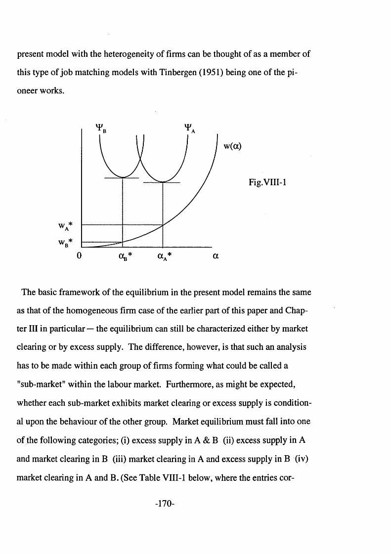
present model with the heterogeneity of firms can be thought of as a member of
this type of job matching models with Tinbergen (1951) being one of the pi
oneer works.
WA*W * B
0 a * a
w(a)
Fig. VIII-1
The basic framework of the equilibrium in the present model remains the same
as that of the homogeneous firm case of the earlier part of this paper and Chap
ter III in particular — the equilibrium can still be characterized either by market
clearing or by excess supply. The difference, however, is that such an analysis
has to be made within each group of firms forming what could be called a
"sub-market" within the labour market. Furthermore, as might be expected,
whether each sub-market exhibits market clearing or excess supply is condition
al upon the behaviour of the other group. Market equilibrium must fall into one
of the following categories; (i) excess supply in A & B (ii) excess supply in A
and market clearing in B (iii) market clearing in A and excess supply in B (iv)
market clearing in A and B. (See Table VIII-1 below, where the entries cor-
-170-

respond to the supply and demand situations of the whole market.)
Sub-market B inS>D S=D
Sub-market A in
S>D (i) S>D (ii) S=DS=D (iii) Not defined (iv) S=D
Table VIII-1 : The characteristics of the market equilibrium
Let us consider these market equilibria in turn. In the following analysis we
define;
Wj** : the equilibrium level of wage for the group i firms
a.** : the ability level at the equilibrium wage, W;** i.e. wi**=w(ai**)
x ** : the equilibrium level of employment of an individual firm in the
group i
n : a number of firms in the group i
Nj** : the total level of employment for the group i at the equilibrium s.t.
Nj’ n x * * with i=A and B
(i) Excess supply in A & B
As the both sub-markets exhibit an excess supply, their optimal wages are the
equilibrium wages. And the equilibrium levels of ability wage and employment
for the two groups, (wA**,NA**,ocA**,) and (wB**,NB**,(XB**), must satisfy the
following;
py'(xA**)=w( a A* *)+cA( aA* *) (VIII-4)
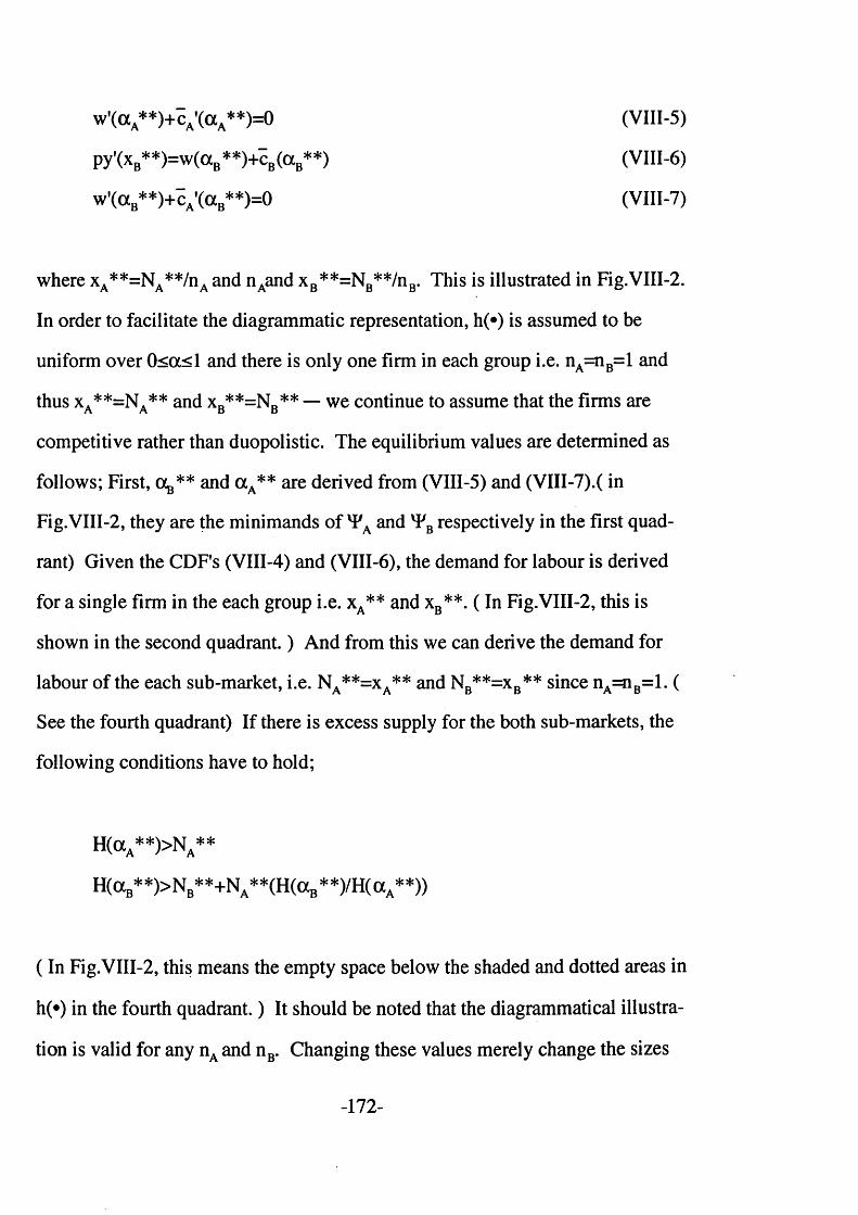
w '(aA**)+cA’(a A**)=0
py’(xB**)=w(aB**)+cB(aB**)
w '(aB* *)+cA’(a B**)=0
(VIII-5)
where xA**=NA**/nA and nAand x B**=NB**/nB. This is illustrated in Fig.VIII-2.
In order to facilitate the diagrammatic representation, h(*) is assumed to be
uniform over 0<oc<l and there is only one firm in each group i.e. nA=nB=l and
thus xa* * = N a ** and xB**=NB** — we continue to assume that the firms are
competitive rather than duopolistic. The equilibrium values are determined as
follows; First, o^** and ocA** are derived from (VIII-5) and (VIII-7).( in
Fig.VIII-2, they are the minimands of *FA and *FB respectively in the first quad
rant) Given the CDF’s (VIII-4) and (VIII-6), the demand for labour is derived
for a single firm in the each group i.e. xA** and xB**. ( In Fig.VIII-2, this is
shown in the second quadrant.) And from this we can derive the demand for
labour of the each sub-market, i.e. NA**=xA** and NB**=xB** since nA i B= l. (
See the fourth quadrant) If there is excess supply for the both sub-markets, the
following conditions have to hold;
( In Fig.VIII-2, this means the empty space below the shaded and dotted areas in
h(*) in the fourth quadrant.) It should be noted that the diagrammatical illustra
tion is valid for any nA and nB. Changing these values merely change the sizes
H(oca**)>Na**
H(ocb* *)>Nb* *+Na* *(H(ccb * *)/H( a A* *))
-172-
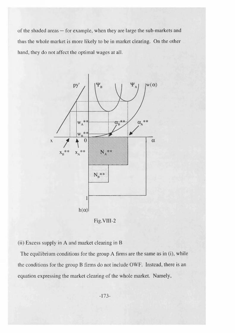
of the shaded areas — for example, when they are large the sub-markets and
thus the whole market is more likely to be in market clearing. On the other
hand, they do not affect the optimal wages at all.
|w (a)
x
h(a)
Fig.VIII-2
(ii) Excess supply in A and market clearing in B
The equilibrium conditions for the group A firms are the same as in (i), while
the conditions for the group B firms do not include OWF. Instead, there is an
equation expressing the market clearing o f the whole market. Namely,
-173-

py'(xA**)=w(aA**)+cA(aA**)
w’(a A**)+cA'(aA**)=0
py'(xB**)=w(aB**)+cB(aB**)
H (aB**)=NB**+NA**(H(aB**)/H(aA**)) (VIII-8)
where xA**=NA**/nA and nAand xB**=NB**/nB Fig.VIII-3 shows how the
equilibrium is reached. Suppose first that the two groups of firms offer their
optimal wages i.e. the group A firms offering wA** and the group B firms
offering wB*, the optimal wage(cf. the first quadrant). This will generate the
labour demand of xA** and xB° for a single firm in each group, (cf. the second
quadrant). This means in turn for the each sub-market the labour demand of
Na** and Nb°. However, this gives excess demand for labour for the whole
market for the wage below wB* — this is indicated by the "double shaded" area
in the fourth quadrant. The excess demand causes the group B firms' wage offer
to rise above their optimal wage wB* as far as wB**, at which the supply equals
the demand through an increase in the supply (cf. the fourth quadrant) and a
decrease in the demand (cf. the second quadrant). Note here that the equilibri
um in the sub-market A is not affected at all, since its higher wage offer means
no worker chooses a group B firm when he faces the two different wage offers.
(iii) Market clearing in A and excess supply in B
This is not plausible since if the group A firms can clear the market with the
wage wA**, which is above their optimal wage by definition, then no group B
firm can attract any worker with their optimal wage, which is their offer wage
-174-

with excess supply. This is indicated by "Not defined" in Table VIII-1.
|w(a)
W,B
N **
Fig.VIII-3
(iv) Market clearing in A and B
Suppose first that the sub-market A is in market clearing at wage wA+, which
is higher than the optimal wage wA* by definition. Then no group B firm can
attract any worker at its optimal wage wB*, since w A+>wA*>wB* and whoever
willing to work at w B* is already employed by a group A firm as there is no
-175-
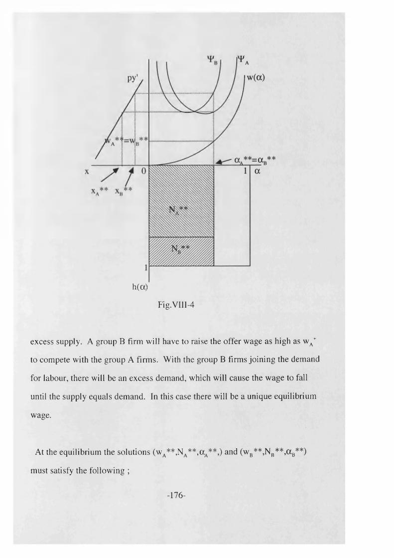
h(a)
Fig.VIII-4
excess supply. A group B firm will have to raise the offer wage as high as wA+
to compete with the group A firms. With the group B firms joining the demand
for labour, there will be an excess demand, which will cause the wage to fall
until the supply equals demand. In this case there will be a unique equilibrium
wage.
At the equilibrium the solutions (w A**,NA**,ccA**,) and (w B**,NB**,ocB**)
must satisfy the following ;
-176-
py'(xA**)=w(aA**)+cA(aA**)
py'(xB**)=w(aB**)+cB(aB**)Na* *+Nb **=H(aA**)
(VIII-10)
where xA**=NA**/nA and nAand xB**=NB**/nB and (VIII-10) indicates a single
equilibrium wage. This is illustrated in Fig.VIII-4. Note that at a A** *FA and
*FB are positively sloped (cf. the first quadrant), implying that no excess supply
exists. This also means NA**+NB**=H(ocA**) (cf. the fourth quadrant)
(2) The Training Cost Function and Multiple Wage Equilibrium
In Chapter VII, we have shown that a steeper c( •) and thus a steeper c (#) tends
to cause the market equilibrium to be characterized with the excess supply of
labour under the assumption of homogeneous firms i.e. uniform c(*). What
effects could generally steeper c(*)'s and thus c(*)'s have on the market equilibri
um when firms are heterogeneous within a market, i.e. when c(*) differs among
the firms ?
We can answer this question in two ways, both of which would simply be
derived as corollaries to what we have just found. Firstly, there is a question
concerning each group of firms within a market. It was shown that the steeper
c(*) is relative to others the higher the optimal wage would be and thus the more
-177-

likely it is to have a job queue i.e. excess supply.
Secondly, let us consider two different markets each of which consists of
heterogeneous firms in the present sense. A market whose firms are generally
characterized by steep c(*) is more likely to be in excess supply equilibrium and
hence to be characterized by a multiple wage equilibrium, the wage being the
optimal wages of each firm. On the other hand, a market whose firms are
generally characterized by flatter c(*) is more likely to be in a market clearing
and single wage equilibrium.
(3) Comparative statics
We shall examine the effect of a change in product demand on the levels of
equilibrium wage and employment by looking at two types of price change.
Firstly, we look at the effect of the product price change on equilibrium in a
market with two groups of firms, who are competitors in the same product
market, i.e. there is a unique product price p, that changes. Secondly, we allow
the two groups to be suppliers of different products, whose prices are pA and pB.
In this latter case, our aim is to examine the comparative statics of a change in
only one of the two product prices.
(a) The effect of a product price change in a single industry case
It was shown that the market equilibrium for the two-group case is character
ized by one of the following.
-178-
(i) Excess supply equilibrium with both firms facing an excess supply.
(ii) Market clearing equilibrium with the group A firm facing excess
supply and the group B firm facing market clearing.
(iii) Market clearing equilibrium with both firms facing market clearing.
In terms of the product price, (i) is likely to occur with relatively low p, (iii)
with relatively high p, while (ii) is the intermediate case. An equilibrium wage
locus in terms of the product price p is illustrated in Fig.VIII-5(a), with the areas
with numbers corresponding to the above three types of the equilibrium, and p,
and p2 signifying the product prices above which the group B firms and the
group A firms face market clearing levels of labour supply respectively. It is
worthwhile mentioning that as the product demand increases the wage dif
ferential, wA**-wB** narrows down, with its upper and lower bounds being
w a* " w b * anc*zero respectively and with the wage offer of the steeper c(*) group
being more rigid. Furthermore, the closer the slopes of cA(*) and cB(*) are, the
closer wA* and w B* are, and the more rigid wB* is. (i.e. (ii) is less likely to
occur) ( See Fig.VIII-5(b) in comparison with (a ) ).
The argument may be extended to a case of multiple optimal wage equilibri
um. (Fig.VIII-6(a) illustrates a case of five groups of firms with each having
distinct optimal wage Wj* with i=A,B,C,D,& E s.t. wA*> wB*>wc*>wD*>wE*)
Again they are assumed to be competitive. The loci are derived in a following
manner. Suppose first that at 0<p<pj the level of labour demand is low enough
for all of the five groups of the firms to be in excess supply in their sub-markets.
-179-
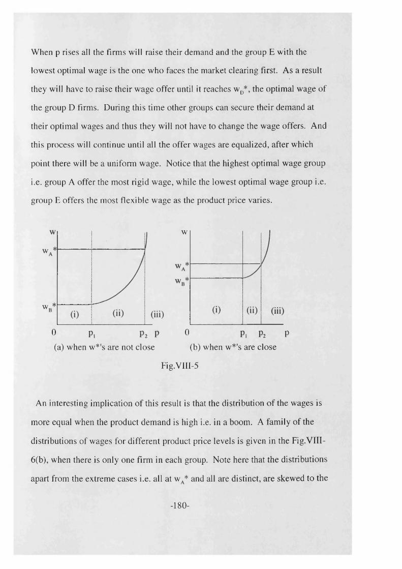
When p rises all the firms will raise their demand and the group E with the
lowest optimal wage is the one who faces the market clearing first. As a result
they will have to raise their wage offer until it reaches w D*, the optimal wage o f
the group D firms. During this time other groups can secure their demand at
their optimal wages and thus they will not have to change the wage offers. And
this process will continue until all the offer wages are equalized, after which
point there will be a uniform wage. Notice that the highest optimal wage group
i.e. group A offer the most rigid wage, while the lowest optimal wage group i.e.
group E offers the most flexible wage as the product price varies.
w
w
w
0 0 P(a) when w*'s are not close (b) when w*'s are close
Fig.VIII-5
An interesting implication o f this result is that the distribution o f the wages is
more equal when the product demand is high i.e. in a boom. A family o f the
distributions o f wages for different product price levels is given in the Fig.VIII-
6(b), when there is only one firm in each group. Note here that the distributions
apart from the extreme cases i.e. all at wA* and all are distinct, are skewed to the
-180-

right. Although one has to be careful when deriving a hypothesis to explain the
real world phenomenon from a simplified model, it is worthwhile noting that a
similar skewness is observed with the distribution of personal income in the real
world. The skewness is often explained in relation to a normally distributed
ability — what is known as "Pigou paradox" that a normally distributed ability
does not generate a normally distributed income but a Pareto or lognormal
distribution o f income. In the present model the skewness came from a uniform
ly distributed optimal wages as opposed to Roy(1950) but with more elements
of econom ics than Champernowne(1953). (See Chapter II(2)(iv)) Indeed it is
important because this derivation takes into consideration the demand side o f
the market.
w
w
w
W,
W
w
(a) Equilibrium wage loci
firms
P
(b) Equilibrium wage distribution
Fig.VIII-6
So far we have not specified which equilibrium among the three (i.e. (i) (ii)
and (iii)) a market is actually in. This can only be determined ex post by observ
ing the behaviour o f the wage when the product price change actually occurs.
-181-
However, it is plausible to state that in the market where c(*) is generally steep
the market is more likely to be in the excess supply equilibrium and vice versa.
Within the same industry, the different steepness of c(*)'s among the firms is
best interpreted as the difference of the system of training workers of the firms.
Firms with steep c(*)'s think that the opportunity wage of a worker (defined as
his productivity in an alternative job such as in a self-employment sector) is a
quite reliable proxy to his training cost and vice versa. The following example
might help the reader to verify this point. Assume that the opportunity wage
reflects one's productivity in a self-employed sector, in which strong individuali
ty rather than conformity counts. Then a firm in which workers are trained
individually may be categorized as having a steep c(*) since it means to value
workers with high opportunity wages highly, while a firm with a mass training
scheme may be categorized as having a flatter c(#). We might label the former
a "specialist firm" and the latter a "generalist firm" — here we do not employ the
terms skilled and unskilled labour as in the previous chapter, to illustrate that
the difference of c(*) is due to difference in OJT process rather than that in skill
level.
With these labelling, the results in the section can be rephrased as;
(1) Generalist firms offer lower wages than specialist firms.
(2) A wage offer of generalist firms is more flexible.
It should be noted that whether these two types of firms co-exist depends on
two things. At a theoretical level, their profit levels must be such that it does
-182-

not pay a firm to change its OJT method because of a certain fixed cost of
starting a new OJT scheme, as different OJT method could mean different profit
level. At a more practical level, they often co-exist as the values that workers
put on the work, be it monetary or non-monetary, differ among them. We do
not analyse in detail this latter aspect in the present paper, since here the utility
functions of workers are assumed to be identical and are functions of the present
wage only.
(b) The effects of a product price change in a multi-industry case
So far we have limited our analysis to a labour market for one industry or
firms competing in the same product market. In this section we consider a
labour market where the demand comes from more than one industry. Conse
quently, the different c(*) may be the result of different types of skills required
in different industries. It also needs to be pointed out that there are more than
one product price that could change when considering comparative statics. We
examine the effect of a change in product prices pA and pB on equilibrium in
turn.
(i) A change in pA
Assume that the both groups are facing excess supply. An increased labour
demand for the group A firms will be met initially by using up the excess sup
ply at the beginning without a wage increase. Once the excess supply is exhaust
ed, wA** starts attracting the workers who would otherwise work for a group B
firm. This will cause the group B firms to raise their wage offer above their
optimal wage wB*.
-183-
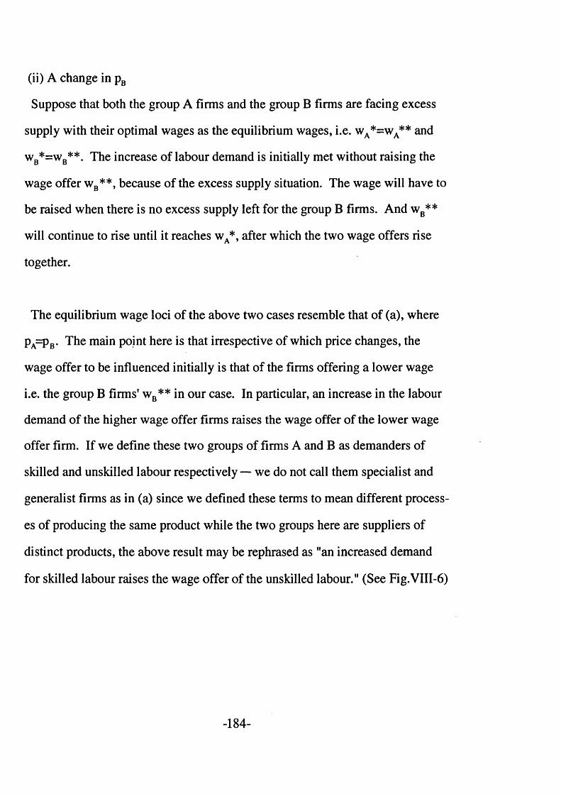
(ii) A change in pB
Suppose that both the group A firms and the group B firms are facing excess
supply with their optimal wages as the equilibrium wages, i.e. wA*=wA** and
wB*=wB**. The increase of labour demand is initially met without raising the
wage offer wB**, because of the excess supply situation. The wage will have to
be raised when there is no excess supply left for the group B firms. And wB**
will continue to rise until it reaches wA*, after which the two wage offers rise
together.
The equilibrium wage loci of the above two cases resemble that of (a), where
pA=pB. The main point here is that irrespective of which price changes, the
wage offer to be influenced initially is that of the firms offering a lower wage
i.e. the group B firms' wB** in our case. In particular, an increase in the labour
demand of the higher wage offer firms raises the wage offer of the lower wage
offer firm. If we define these two groups of firms A and B as demanders of
skilled and unskilled labour respectively —■ we do not call them specialist and
generalist firms as in (a) since we defined these terms to mean different process
es of producing the same product while the two groups here are suppliers of
distinct products, the above result may be rephrased as "an increased demand
for skilled labour raises the wage offer of the unskilled labour." (See Fig.VIII-6)
-184-
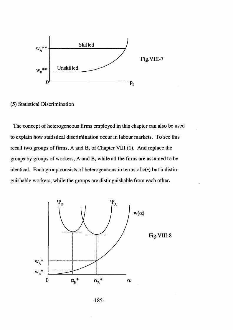
w ** Unskilled
Skilled
Fig.VIII-7
B
0
(5) Statistical Discrimination
The concept of heterogeneous firms employed in this chapter can also be used
to explain how statistical discrimination occur in labour markets. To see this
recall two groups of firms, A and B, of Chapter VIII (1). And replace the
groups by groups of workers, A and B, while all the firms are assumed to be
identical. Each group consists of heterogeneous in terms of c(*) but indistin
guishable workers, while the groups are distinguishable from each other.
w *B
wA*
w(a)
Fig.VIII-8
0 (Xb* aA* a
-185-

Fig.VIII-8 illustrates how the discrimination would take place. The firm faces
two groups of workers whose average labour cost are given by
vFA(a)= w(a)+cA(a) and 'F B(a)=w(a)+cB(a)
The firm would offer the wage that minimizes the labour cost i.e. wA*. Howev
er, in order to secure the minimum labour cost it needs to refuse all the group B
applicants, since a typical group B worker attracted by wA* has a much higher
expected labour cost. This is the case of statistical discrimination, since not all
workers in the group B are less productive than those in the group A and yet
they are refused. Such discrimination may be dealt with by an anti-
discri mi nation legislation appealing for an equal opportunity to all. However,
this will force the firms away from the optimal point. The better remedy lies in
the change of ability distribution of the group B through education so that the
firms do not find it profitable to discriminate against the group B.
(6) Policy Implications
There are three main policy implications that can be drawn from the results
obtained in this section. The first is concerned with non-uniformity of the
equilibrium wage. In a simple neo-classical framework, the existence of multi
ple wage may be explained as a result of a luck of information on the wage
variation or a lack of competition among the firms to eliminate the variation. In
the present approach, instead, it was shown that multiple wage is possible at the
equilibrium, when the firms are heterogeneous, with the heterogeneity being
expressed here in terms of different OJT cost among the firms. It was also
-186-

noted that the multiplicity would be more likely in a market where labour traded
is mostly skilled. Hence the resulting unequal distribution of labour earnings
can not be eliminated by making available the information on the wage vari
ation or by encouraging the competition among the firms. As the multiplicity
comes from the heterogeneities in both workers and the firms, the most effec
tive policy to eliminate the inequality would be to eliminate the heterogeneities
themselves. As for the firms, this means for all the firms to have an identical
training cost function so that the optimal wage is unique to all the firms. Or the
government may be able to tax or subsidize the firms on their training cost to
uniformalize the optimal wage. As for the firms, this would mean to, for exam
ple, recommend to all the firms to pursue the same OJT. As for the workers, the
opportunity wage has to be uniformalized among the potential workers by
means of educational planning. This would supplement the training as post-
educational investment. .
The second is concerned with the distribution of labour earnings and business
cycle. The labour earnings are distributed more equally during booms with high
labour demand and more unequally during slumps with low labour demand
— the second part of Kuznet's Reversed U shape hypothesis i.e. after some spell
of income unequalization, economic growth will eventually bring about the
equality. (See Kuznets (1963)) Thus the redistribution of income through
taxation is most needed when it would hurt the economy most, rather than when
the economy can afford to be generous to the less fortunate members of the
society.
-187-

Thirdly, the wages are not determined by equating supply and demand unless
the market is in market clearing equilibrium and hence the wage differential is
the direct result of the production process and in particular of the OJT. There
fore those wage differentials can not be eliminated or eased by controlling the
supply of or demand for various types of labour, as is the case for neo-classical
models of labour markets. So, for example, a rise in demand for skilled labour
raises the wage of unskilled labour first and thus reduces the wage differential,
while in a neo-classical model this would widen the wage differential.
In this chapter, we have established the following ;
Firstly, we have shown that when firms are heterogeneous within a market in
terms of c(*) a multiple wage equilibrium is possible. The necessary condition
for the multiple wage equilibrium to occur is that the firm with the highest wage
offer faces an excess supply of labour. Conversely for the highest wage offer
firm to be in market clearing means that the whole market is in market clearing
equilibrium and with its wage being the single equilibrium wage.
Secondly, with comparative static analysis it was shown that in a multiple
equilibrium situation, the lower the wage is relative to other offers the more
flexible it is as the product demand fluctuates. Also the theoretical model
suggests that the distribution of wages is skewed to left just as the real world
income distribution shows, with it becoming more equal in booms and less
-188-
equal in slumps.
Thirdly, with different types of industries acting as demanders of labour in the
same labour market, wage offers for skilled labour tends to be more rigid than
those for unskilled labour. Whichever product it may be, a change in its de
mand affects most the wage offer of the most unskilled labour. In particular, a
rise in demand for products for which a skilled labour is required will first raise
the offer wage of unskilled labour. The rational behind this result is that the
demanders of the unskilled labour have to raise the wage to make up for the
labour supply taken away by the skilled labour demanders.
Fourthly, the model was used to explain how statistical discrimination could
occur. It was pointed out that an anti-discrimination legislation to give equal
opportunity to all would force the firms away from the optimal point and thus
some other policy to change the ability distribution of the discriminated group
would be more advisable.
Finally, some policy implications were drawn. The multiple wage is not a
market failure and thus the policy to eliminate it would require basic revisions
of supply of and /or demand for labour. The equity measure is more important
in slump than in booms. And lastly the wage of unskilled labour is affected and
is so first by a change in demand for any type of labour.
-189-

CHAPTER IX OBSERVATIONALLY DISTINGUISHABLE WORKERS
(1) Introduction
So far we have been assuming that ability of each worker is not observable to
the firm at the time of contract. Indeed, this was the crucial assumption in
explaining as to why the workers are paid uniformly despite their heterogeneity
in the earlier model. In reality, however, it is more likely that the ability of each
applicant is known to the recruiting firm at least partially. Recall the excess
supply equilibrium we have described earlier on. If a firm can select workers
from those willing to work at the optimal wage rather than picking them at
random, it will rank and recruit workers according to the ability level, because
the total training cost would be reduced. This in turn raises the employment
level.. Thus it is the interest of the recruiting firm to know the ability levels of
the applicants.
Typically, a job opening specifies an offer wage and a minimum hiring stan
dard as well as other aspects of working conditions. This also prompts the
potential workers to reveal their ability — otherwise, they may be considered as
not satisfying the standard and fail to get the job. Hence the distinguishability
becomes an important element for both sides of the labour market. In this
chapter, we examine the mechanism of a labour market, in which observational-
ly distinguishable workers form a job queue by their known ability levels for
jobs specifying the wage offer and the minimum hiring standard. The basic
-190-
framework of this model is unchanged from the indistinguishable workers case
of the earlier chapter. In particular, the recruiting firms offer OJT and the
uniform wage is offered to several openings of an identical job despite the
heterogeneity of the applicants.
There are several theoretical issues to be clarified before we move on to the
analysis. To illustrate them, let us first present an example of a type of a labour
market we have in mind in this chapter. In Japan, where there are more than
500,000 university students graduating in March every year, early summer
months are the busiest time for the final year students with their job search.
Although most of them are lucky enough to secure a job before graduation, this
activity is rather tiresome for the job searching students as well as for the recruit
ing firms, with so many future workers trying to find the ideal post within few
months. To fit in all those, many large firms offer tens or even hundreds of the
same job openings and give them OJT. Typically, the job applicants experience
a three-stage recruiting procedure by a firm. At the first stage, screening by
educational credentials singles out the applicants with good academic achieve
ments as well as from universities of relatively high reputation. The successful
applicants are then invited to take a short test, in which general rather than
specific knowledge is asked. This may be repeated and by the end of this stage
the number of applicants is greatly reduced. An interview or several interviews
are held in the last stage of the recruitment for the group of applicants already
small enough to make more detailed and personal evaluations. The applicants
are asked to express their commitment to the firm, the fellow employees and to
the job itself. If the interviews are repeated, the interviewers are upgraded in
-191-

the firm’s hierarchy each time.
The newly recruited workers, who are relatively homogeneous by age will
receive OJT, a training necessary to adapt them to the new working environ
ment. This will then be followed by a promotion race. In Japan, the path to the
promotion is known to be quite long compared to those in other developed
countries. Koike (1991) argues, for example, that the major promotion for
university graduates could take place as late as 15 years after the recruitment.
Several remarks may be made about this example. Firstly, the competitions
for jobs is hard and tiresome not because of large excess supply of labour but
because each graduate applies to many firms. In a way such a search strategy is
not meaningless, as the firms see the educational achievement as an indicator of
trainability rather than immediate productive quality in its own right — in
general it is more so for students of non-pure science courses than to those of
science courses but the former group is much larger. Furthermore, the ranking
table of universities makes university entrance extremely competitive. And this
makes many families start investing in education of their children at a much
earlier stage. Many educationalists hold the opinion that such an interest in
education is rather overheated, and these selected graduates are not always so
much more productive than others since academic achievement is not the only
quality needed for job performance. In fact some firms, notably Sony already
for some years, do not ask the applicants which university they graduated from.
But it has not yet become the standard procedure. ( See Takeuchi (1995) for
more extended analysis. He provides extremely useful information on this
-192-
issue. I do not deal with it here mainly because it is more of a sociological
approach and thus would not be directly relevant to the present analysis.)
Secondly, despite a decade or more that the workers have to wait to receive
what they deserve, the quit rate is not known to be particularly high in Japan
compared with other developed countries. ( See Koike (1991)) This is puz
zling, at least theoretically, since one might expect the workers to quit to move
to other job or where he can be paid what he thinks is worth right away. Con
trast this type of turnover with the relationship between training and job tenure
discussed earlier in Chapter II and Chapter V. It was about evaluating productiv
ity of workers over time in the world of homogeneous labour, while here we are
concerned with evaluating workers of homogeneous ability. There are several
reasons for not paying the wage according to one’s productivity even if the
individual difference is known by the educational credentials. Firstly, it would
be too tedious and costly to derive an individual wage scheme for everyone
recruited to the same job — the productivity difference among the recruits may
be too insignificant especially in our example. To the extent that OJT is a group
activity, it might be difficult to determine the individual OJT cost — the firm
may know the total OJT cost instead. Put it differently, firms are not likely to
adjust the wage to individual recruits who are expected to perform the same
task. There are cases where the wage may be set according to one’s productivi
ty. For example, an already highly skilled worker may negotiate his wage to
fully reflect his productivity. But it is a different type of labour market all
together from our case of recruiting inexperienced workers to train them to be
skilled. And even for our highly skilled worker the wage will be associated to
-193-

the job characteristics or grade — the firm would claim that the employee
receives £ x per month say, because he performs a job of the grade y say, which
generates the productivity worth £ x, rather than because his productivity is
worth £ x. The best way to imagine it is that workers are allocated to already
existing job slots and there is not always a slot for everyone. Extended discus
sions on such an issue are found in the job evaluation literature in the manage
ment science — see, for example, Patten (1977) for an introductory reference,
but often their arguments are not based on economic theories.
There is also a question of an accuracy of the screening — the educational
credentials need to be complemented by short tests and interviews, because it is
not considered to be the perfect screening device. After all, the best way to
screen is monitoring on the job. It may not be a good idea to determine one’s
wage fully based on the pre-employment information, which is not perfect.
That this inaccurately measured wage can affect one’s incentive to work is
another reason for the uniform wage. ( See Patten (1977)) Think of the recruit
ment as the starting point of a promotion race. It would be the interest of the
firm to organize a fair race starting with the same wage and rewarding later on
properly reflecting the achievement of each participant.
One might also wonder what happens to those unsuccessful applicants i.e.
those with the credentials below the minimum hiring standard. Can they, for
example, improve the chance of recruitment by offering to work at a lower
wage? Recall that in the indistinguishable workers case, the further attempt of
unsuccessful applicants by offering to work at a lower wage is not effective as
-194-

this merely acts to reveal their low level of ability. When the ability is observ
able, the wage offer of those unsuccessful applicants will be bid down to their
own opportunity wages as the firms are assumed to know w(a). As this is the
wage they can earn in the alternative sector, they do not find worthwhile to seek
an employment in this firm. Notice that this argument is valid provided that the
successful applicants are paid the uniform wage, the assumption supported by
the earlier remarks of this chapter. Thus as long as the uniform wage is main
tained by the reasons explained earlier, no once-unsuccessful applicant can
make it with the second attempt by undercutting his offer wage.
The model of this chapter is a simplified version of such a process of recruit
ment, OJT and promotion as described by the Japanese example. Thus the
model is particularly relevant to the labour market for new recruits who require
training , and not for already skilled workers. In this model ‘qualification’, the
educational credential, is the only screening device and there is no short test or
interview. The underlining assumption is that the qualification is not perfect but
superior at least to the other two. Secondly, it is a one-period model with
recruitment and OJT but without promotion. A multi-period model with promo
tion races would be more complete and appropriate particularly for dealing with
the incentive aspect. However, we stay with the one-period model in order to
concentrate on the adverse selection aspect of the labour market model in rela
tion to the heterogeneity of labour. The equilibrium will be described by a
market clearing situation for the workers with the qualification range covered
between the wage offer, i.e. the qualification of the workers whose opportunity
wage is the optimal wage, and the minimum hiring standard. And those below
-195-

the minimum hiring standard forming the excess supply.
(2) The Model
Recall the set of profit maximization conditions for the model with indistin
guishable workers,
py’(xd)=c(a)+w(oc) (HI-7)
?(a)+w '(a)=0 (III-8)
from which a* and x* are derived for the excess supply equilibrium. And the
profit is,
7U,=py(x*)-[w*(a*)+c(<x*)]x* (IX-1)
It follows from this that if the firm can choose a particular group of x* workers
out of the pool of workers at w* by setting a minimum hiring standard a , its
profit would be increased. This is because selecting the better x* workers in
such a way from the pool of workers would imply,
7i„=py(x*)-[w*(a*)+c(a,a*)]x* (IX-2)
J c(z)h(z)dz where c(a,a)= and oc=a*
Jh(z)dz
-196-
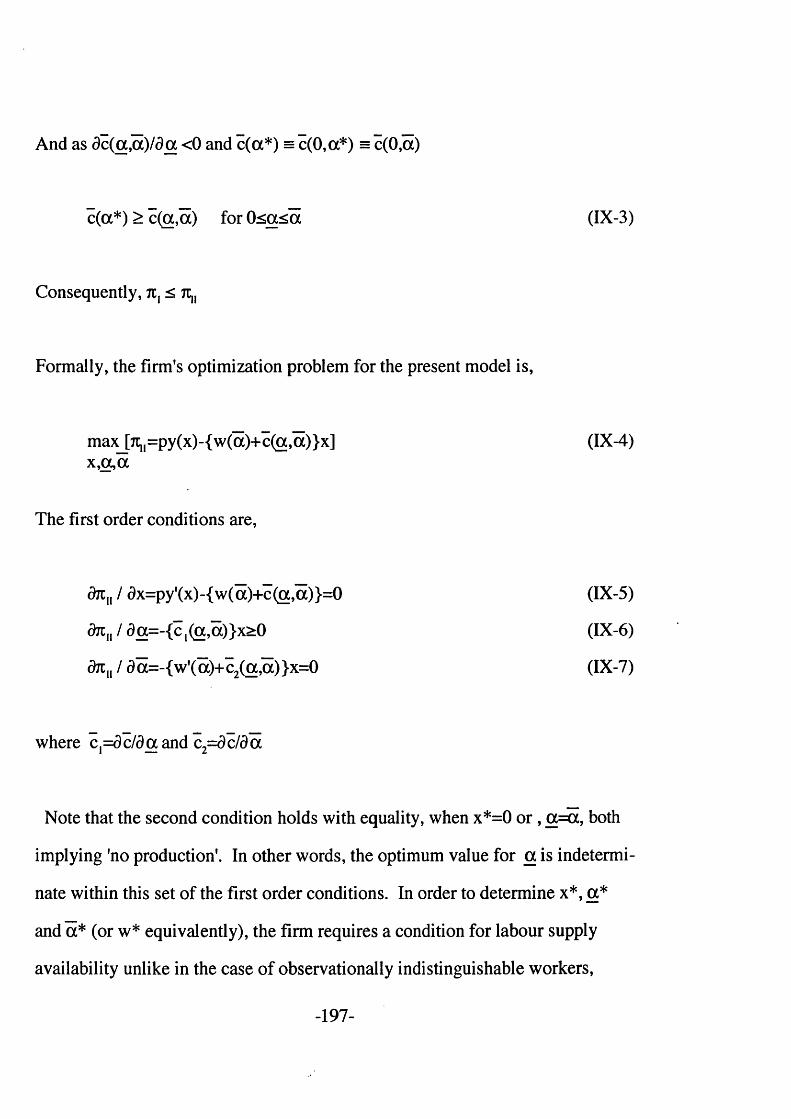
And as dc(a,cc)/doc <0 and c(a*) = c(0,a*) = c(0,oc)
c(a*) > c(a ,a) for 0 < a< a (IX-3)
Consequently, 7C, < 7C,,
Formally, the firm's optimization problem for the present model is,
max_[7CII=py(x)-{w(a)+c(a,a)}x] (IX-4)x ,a ,a
The first order conditions are,
drc,, / dx=py'(x)-{w(oc)+c(a,a)}=0
dKn / da= -{c1(a,a)}x>0
dKn / da=-{w '(a)+c2(a,a)}x=0
where c,=dc/daand c2= d d d a
Note that the second condition holds with equality, when x*=0 or , a= a , both
implying 'no production'. In other words, the optimum value for a is indetermi
nate within this set of the first order conditions. In order to determine x*, a*
and a* (or w* equivalently), the firm requires a condition for labour supply
availability unlike in the case of observationally indistinguishable workers,
-197-
(IX-5)
(IX-6)
(IX-7)

where it comes to the market with their desired levels of wage and the employ
ment. The first and the third together would be equivalent to the conditions for
the case of observationally indistinguishable workers if a=0. Consequently the
third condition does not necessarily hold with equality either just as for a market
clearing case of the previous model.
The optimum values x*, a* and a* are determined as the market equilibrium
values such that,
where, as in the indistinguishable workers' case, H (0 is the portion of the
labour supply that is available to one firm.
These three conditions imply in turn;
(i) the marginal productivity is equal to the marginal labour cost
(ii) the marginal labour cost with respect to a is non-positive.
(iii) supply equals demand
And unlike the indistinguishable workers' case, they will have to be determined
simultaneously. Recall that (IX-9) depends on a as well as a . Although there
is no excess supply equilibrium in the sense described earlier, the equilibria
should be categorized into two types in terms of the value of a — a>0 means it
py'(x)={w(a)+c(a,a)}
w'(a)+c2(a,a)<0
H(a)-H(a)=x (IX-10)
(IX-8)
(IX-9)
-198-
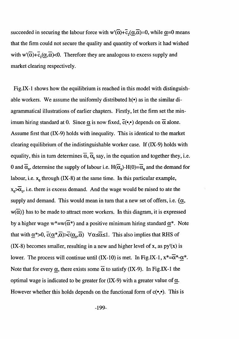
succeeded in securing the labour force with w'(oc)+c2(a,a)=0, while a=0 means
that the firm could not secure the quality and quantity of workers it had wished
with w'(cx)+c2(a,a)<0. Therefore they are analogous to excess supply and
market clearing respectively.
Fig.IX-1 shows how the equilibrium is reached in this model with distinguish
able workers. We assume the uniformly distributed h(*) as in the similar di
agrammatical illustrations of earlier chapters. Firstly, let the firm set the min
imum hiring standard at 0. Since a is now fixed, c (v ) depends on a alone.
Assume first that (IX-9) holds with inequality. This is identical to the market
clearing equilibrium of the indistinguishable worker case. If (IX-9) holds with
equality, this in turn determines a , say, in the equation and together they, i.e.
0 and a 0, determine the supply of labour i.e. H(oc0)-H(0)=a0 and the demand for
labour, i.e. x0 through (IX-8) at the same time. In this particular example,
x0> a0, i.e. there is excess demand. And the wage would be raised to ate the
supply and demand. This would mean in turn that a new set of offers, i.e. {a,
w(a)} has to be made to attract more workers. In this diagram, it is expressed
by a higher wage w*=w(a*) and a positive minimum hiring standard a*. Note
that with a*>0, c(a*,a)>c(a0,a) V a < a ^ l. This also implies that RHS of
(IX-8) becomes smaller, resulting in a new and higher level of x, as py'(x) is
lower. The process will continue until (IX-10) is met. In Fig.IX-1, x*=oc*-a*.
Note that for every a , there exists some a to satisfy (IX-9). In Fig.IX-1 the
optimal wage is indicated to be greater for (IX-9) with a greater value of a .
However whether this holds depends on the functional form of c (v ) . This is

discussed later.
What is established here is that involuntary unemployment can exist at the
equilibrium just as for the models o f the earlier chapter with indistinguishable
workers. But here the unemployed are not randomly chosen from those willing
to work at the offer wage but they are the workers with their ability lower than
the minimum hiring standard. In fact the indistinguishable workers' case may
be thought o f as a constrained case o f the present model, with the constraint
being a^O. The type o f a labour market that is likely to exhibit the excess
supply equilibrium is the same as the earlier model. Hence, the minimum
qualification is more likely to exist in a skilled job market, in which excess
supply is more likely, than in an unskilled job market.
Fig.IX-1
(3) Comparative statics
-200-
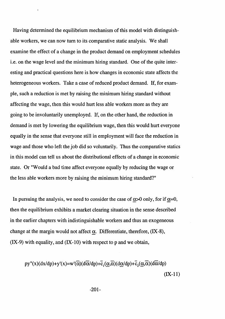
Having determined the equilibrium mechanism of this model with distinguish
able workers, we can now turn to its comparative static analysis. We shall
examine the effect of a change in the product demand on employment schedules
i.e. on the wage level and the minimum hiring standard. One of the quite inter
esting and practical questions here is how changes in economic state affects the
heterogeneous workers. Take a case of reduced product demand. If, for exam
ple, such a reduction is met by raising the minimum hiring standard without
affecting the wage, then this would hurt less able workers more as they are
going to be involuntarily unemployed. If, on the other hand, the reduction in
demand is met by lowering the equilibrium wage, then this would hurt everyone
equally in the sense that everyone still in employment will face the reduction in
wage and those who left the job did so voluntarily. Thus the comparative statics
in this model can tell us about the distributional effects of a change in economic
state. Or "Would a bad time affect everyone equally by reducing the wage or
the less able workers more by raising the minimum hiring standard?"
In pursuing the analysis, we need to consider the case of oc>0 only, for if a=0,
then the equilibrium exhibits a market clearing situation in the sense described
in the earlier chapters with indistinguishable workers and thus an exogeneous
change at the margin would not affect a . Differentiate, therefore, (IX-8),
(IX-9) with equality, and (IX-10) with respect to p and we obtain,
py"(x)(dx/dp)+y'(x)=wf(a)(da/dp)+c1(a,a)(da/dp)+c2(a,a)(da/dp)
(IX-11)
-201-

w"(oc)(da/dp)+c2,(a,a)(da/dp)+c22(a,a)(da/dp)=0
h(a)(da/dp)-h(a)(da/dp)=dx/dp
(IX-12)
(IX-13)
where c21(oc,a)=02c/5a6a and c22(a ,a)= 52c/6oc2
With w '(a)+c2(a,a)=0 at the equilibrium, (IX-11) (IX-12) and (IX-13) may be
written in a matrix form as;
py" 0 -C l dx /d p -y*(x)0 W"-|-C22 C2I d a /d p — 0
_ l -h(cc) h ta). _da/dp_ . 0 .
(IX-14)
And therefore
dx/dp =IA|-' {-yf((w"+c22)h(a)+c2I»h(a))} (IX-15)
doi/dp =IAI'* {-y,#c2l} (IX-16)
da/dp =IAI*‘ {y’(w"+c22)} (IX-17)
where IAI=py"{(w,t+c22)h(a)+c21*h(a)}+(w,,+c22)c], i.e. the determinant of the
matrix of (IX-14)
Among the terms in (IX-15) (IX-16) (IX-17) and IAI, we know;
y’>0, y"<0, w"+c22>0, h(*)>0, Cj<0, c22>0, p>0,
while we do not know the sign of c21. However,
-202-

_ _ _ J c(z)h(z)dzC2|— c21(a ,a ) = d 7c / d a d a = ( d / d a d a ) -^-=----------
Jh(z)dz
= (d /da ) [h(a){c(a)~ c(a,a)}/{H(a)-H(a)}]
= [h(a)/{H(a)-H(a)}2 ][-c,(^a){H (a)-H (a)}+{c<a)-c(a,a)}h(a)]
= [h(oc)h(a)/{H(a)-H(a)}2][c(a)+c(a)-2c(a,a)] (IX-18)
since c,= -h(a){c(a)-c(a,oc)}/{H(a)-H(oc)} (IX-19)
Thus c21>(<)0 if (l/2){c(a)+c(a)}>(<)c(a,a) (IX-20)
It is difficult to say anything precise about the direction of the inequality
without specifying at least functional forms of c(*) and h(*). All that can be said
at this point is that c ( v ) has c(a) and c(a) as its upper and lower bounds respec
tively, with these polar cases representing the limiting cases of h(*) being con
centrated at a and a respectively. Therefore a very high concentration of the
distribution at a would imply c21<0 and at a c2I>0. However, as a and a are not
exogeneously given variables but rather they are endogeneously determined in
the market equilibrium, we can not state whether c21>(<)0 by simply examining
the shape of h(«) in this manner. However, given the sign and the size of c21, the
signs of (IX-15) (IX-16) and (IX-17) can be easily determined. To see this
group the terms which appear in (IX-15) (IX-16) and (IX-17) into the following
four terms — IAI, {-y'((w"+c22)h(qc)+c21*h(a))}, -y'*c2l, and y'(w"+c22). Their
-203-
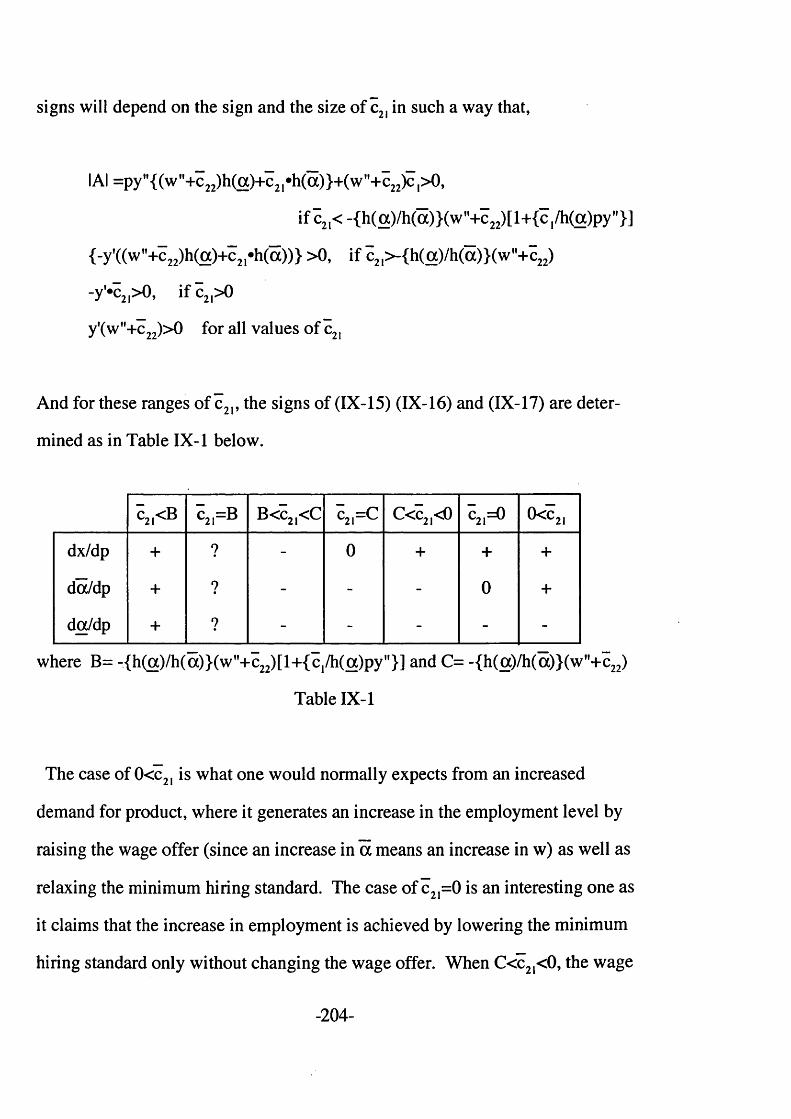
signs will depend on the sign and the size of c2l in such a way that,
IAI =py,,{(w"+c22)h(a)+c21*h(a)}+(w"+c22)c ,>0,
if c2l< -{h(a)/h(a)}(w"+c22)[l+{c,/h(a)py"}]
{-y'((w"+c22)h(a)+c2,*h(a))} >0, if c21>-{h(a)/h(a)}(w"+c22)
-y'*c21>0, if c21>0
y'(w"+c22)>0 for all values of c21
And for these ranges of c21, the signs of (IX-15) (IX-16) and (IX-17) are deter
mined as in Table IX-1 below.
c2,<B c21—B B<c21<C
ull_NI o C<c21<0 c2,=0 0<C2I
dx/dp + ? - 0 + + 4*
da/dp + ? - - - 0 +
da/dp + ? - - - - -
where B= -{h(a)/h(a)}(w"+c22)[l+{c1/h(oc)py"}] and C= -{h(a)/h(a)}(w"+c22)
Table IX-1
The case of 0<c21 is what one would normally expects from an increased
demand for product, where it generates an increase in the employment level by
raising the wage offer (since an increase in a means an increase in w) as well as
relaxing the minimum hiring standard. The case of c21=0 is an interesting one as
it claims that the increase in employment is achieved by lowering the minimum
hiring standard only without changing the wage offer. When C<c2I<0, the wage
-204-

offer is reduced while the employment level is increased, implying that the firm
decides to employ less able but cheaper workers. The cases of B<c21<C and
c2l=C show rather unexpected results that the increased demand for the product
causes the reduction and no change in the labour demand respectively. The
entries for the case of c2l=B mean that they are undefined since this condition
implies IAI=0 and in such a case we can not solve the simultaneous equations
(IX-14). And finally if c21<B, the employment is increased by raising both the
wage offer and the minimum hiring standard, implying that the firm decides to
employ more expensive but more able workers.
In total, the comparative statics results can be almost anything if we do not
restrict the value of c21. On the other hand, it is true that c21 is derived from c(*)
and h(*) which do follow certain behaviour. Let us attempt to illustrate more
explicitly the issue here, by specifying c(*) and h(*) as linear functions such
The second function secures that H (l)= l for all values of a and at the same time
represents linearly increasing/constant/decreasing density functions for neg
ative/zero/positive value of a respectively.
With these specifications,
that;
c(a)=l-a
h(a)= (l-^)+ aa where -2<a<2
(IX-21)
(IX-22)
-205-
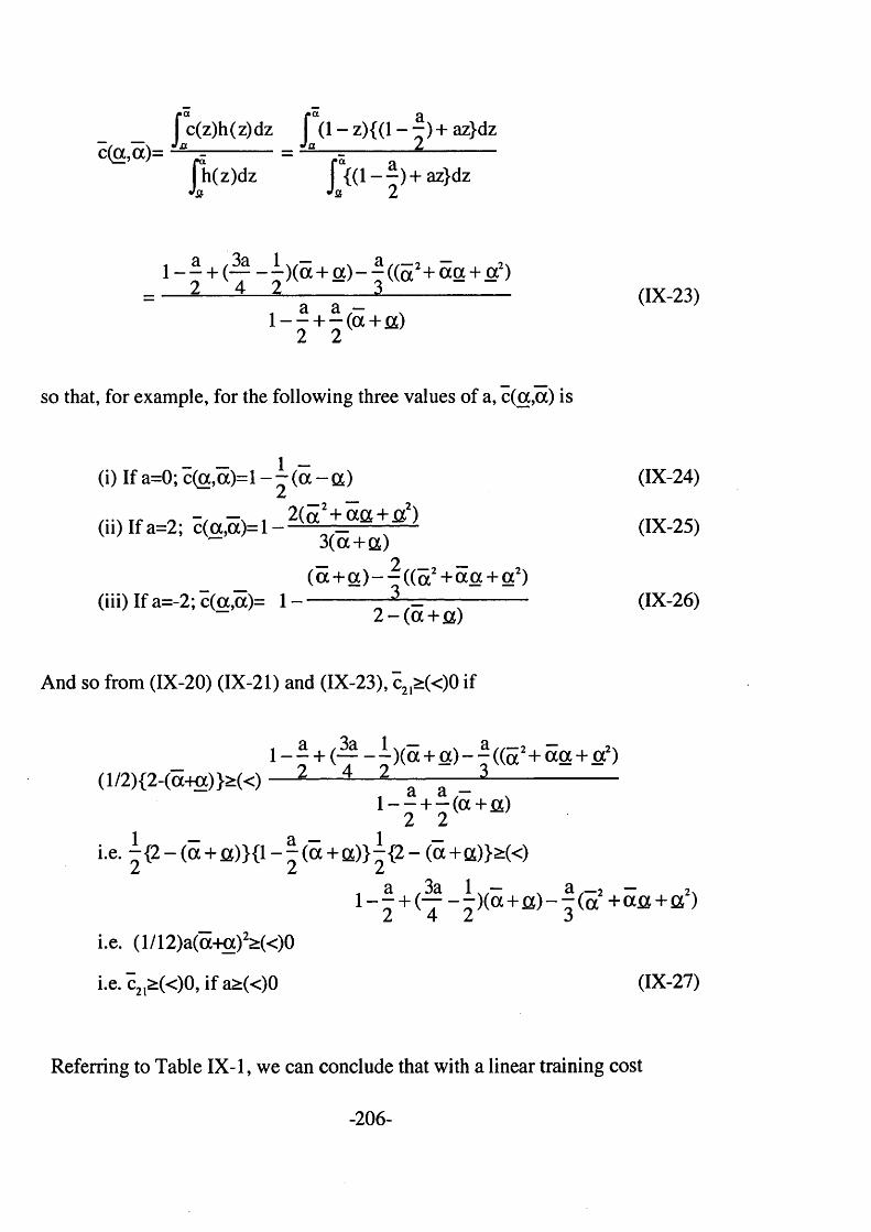
fc(z)h(z)dz f (1 - z){(l - “ ) + az}dzcfa a)= = —— =----------- ----------
fh(z)dz f°{ (l--)+ az} d zJa 2
a2
3a4
I ' " 2
! - - + (— - - ) ( a + a ) - - ( (a 2 + oca + a 2)
a a — x l - - + - ( a + c O
2 2
(IX-23)
so that, for example, for the following three values of a, c(a ,a) is
(i) If a=0; c(a ,a)= l - )- ( a - a) (IX-24)
/ • • \ x r ^ — x 1 2(a2+aa+fic2) / I V n r t(n) If a=2; c ( a ,a ) = l - ------- = -------— (IX-25)3(a+a)
— 2 _ —(a+a)— ((a2+«oc + a2)(iii) If a=-2; c(a,a)= l - ----------- ~ ^ ~ = ---- (IX-26)
“ 2 - ( a + a )
And so from (IX-20) (IX-21) and (IX-23), c2l>(<)0 if
l - - + (— - -)(a + a) - - ((a2+ cxa + a?)(l/2){2-(a-HX) }^«) 2 4 2 ~ _ 3 ---------
l _ _ + _ ( a + a )
i.e. |{2 - (a+a)}{! - |(a + a )}^ {2 - (a+a)}>(<)a /3a l w— N a .—2 — 2\
l - - + (— - “ ) ( a + f l ) - “ ( a + o c £ + a )
i.e. (l/l2 )a (a+ a)2>(<)0
i.e. c2l>(<)0, if a>(<)0 (IX-27)
Referring to Table IX-1, we can conclude that with a linear training cost
-206-

function if the population is concentrated among the more able workers i.e. a>0,
then an increase in the product demand is likely to bring about an increase in the
wage offer and a lowering of the minimum hiring standard. If the population is
concentrated among the less able workers i.e. a<0, then the increase in the
product demand is likely to bring about a lowering of the minimum hiring
standard as before but the wage offer will fall. Finally, if the population has a
uniform distribution of ability i.e. a=0, then the wage offer will be rigid.
How about the convexity of c(*)? Can we say anything about the sign of c21
from the convex shape of c(*) by assumption i.e. T2 in (1) Assumptions of
Chapter III)? In order to examine this, continue to assume the linear h(*) as in
(IX-22) but a strictly convex c(«) as we have already dealt with a linear c(*) i.e.
c(a)= l-a. We would like to verify the sign of c21 or equally from (IX-20) ^
{c(a)+c(a)}>(<)c(a,a). The convexity implies,
1 {c(a)+c(a)}= = 1 — P (B-Az)dz>=-^— f“ c(z)dz (IX-28)2 a - a - k a - a Ja
where B-Aa is a linear function of a , which goes through (a, c(a)) and (a ,
c(a)),(See Fig.IX-2)
Now compare the RHS of (IX-28) and c(a,a),
z J — J c ( z ) d z > ^ — f c(z)dz- - r 1 f c(z)h(z)dz a - a Ja a - a Ja H ( a ) - H t o ) ^
-207-

. (IX-29)
1 r “ 1 1 r “ a== j c(z)dz- —------------ -— — ------- = ------ j c (z )( l- -+ a z )d z
a ~ a “ ( a + a ) { i - - + - ( a + a ) } a ~ a ° 2
r a 1 —aj c (z ){~ (o m -^ )-z }d z
( < x + a ) { l - - | + | ( a + a ) }
As -2<a<2, the denominator is positive unless a = a or a+a=0. And
f c(z){—(a+a)-z}dz>0* a 2
since (i) c(*) is a decreasing function
(ii) ^(oc+a)-a is linear in a , and 0 at cxp=^(a+a) (See Fig.IX-3(a)and(b))
Therefore if a>0,
^{c(a)+c(a)}= ■= f (B-Az)dz>zi f c(z)dz>2 ” a - a Ja
1 . f c(z)h(z)dz=c(a,a) (IX-30)H ( a ) - H to ) Jo
and hence if a>0, c21>0. Note that, on the other hand, a<0 does not necessarily
guarantee c21<0. This rather asymmetric result is due to the convexity of c(») in
a . So these examples show that a positive slope of the population density and a
convexity of the training cost function makes as a more likely outcome an
increase of wage in response to an increase of product demand. (See Table
IX-2)
-208-
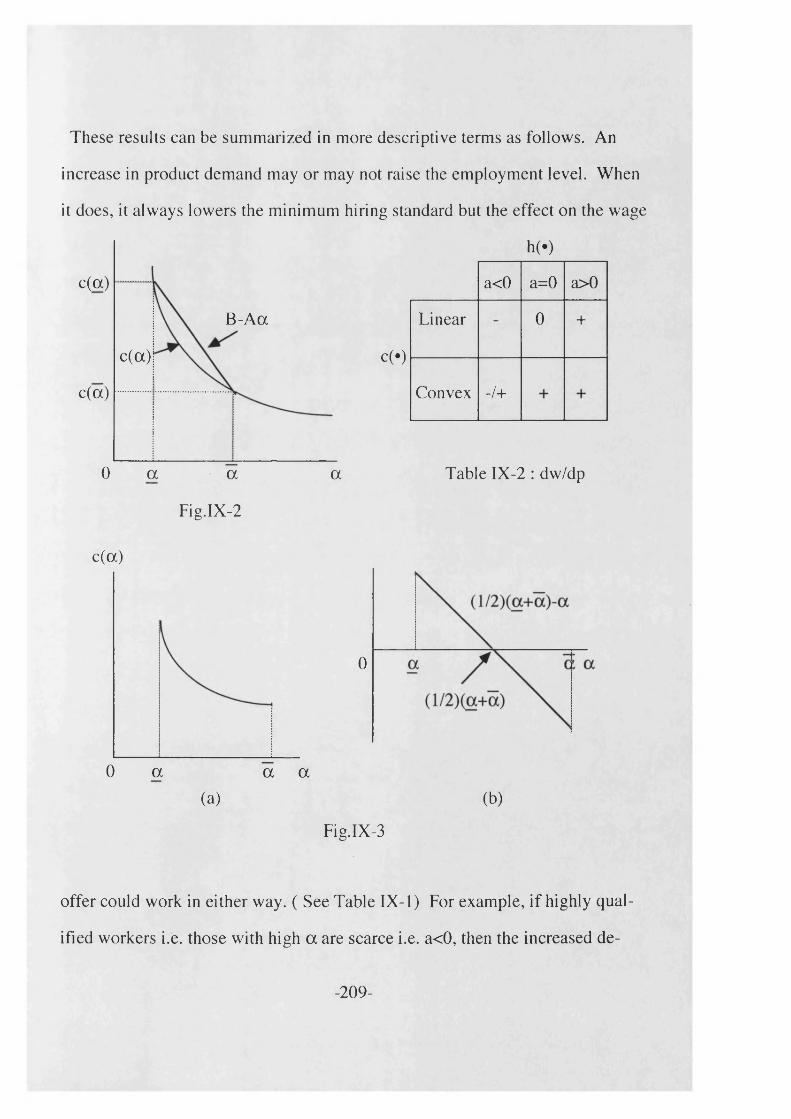
These results can be summarized in more descriptive terms as follows. An
increase in product demand may or may not raise the employment level. When
it does, it always lowers the minimum hiring standard but the effect on the wage
hWc(oc)
B-Aa
c(a)
c(a)
0 a a a
Fig.IX-2
cW
Linear
Convex
a<0
- /+
a=0
0
a>0
+
Table IX-2 : dw/dp
c(a)
0 a oc a
0
(a) (b)
Fig.IX-3
offer could work in either way. ( See Table IX -1) For example, if highly qual
ified workers i.e. those with high a are scarce i.e. a<0, then the increased de-
-209-
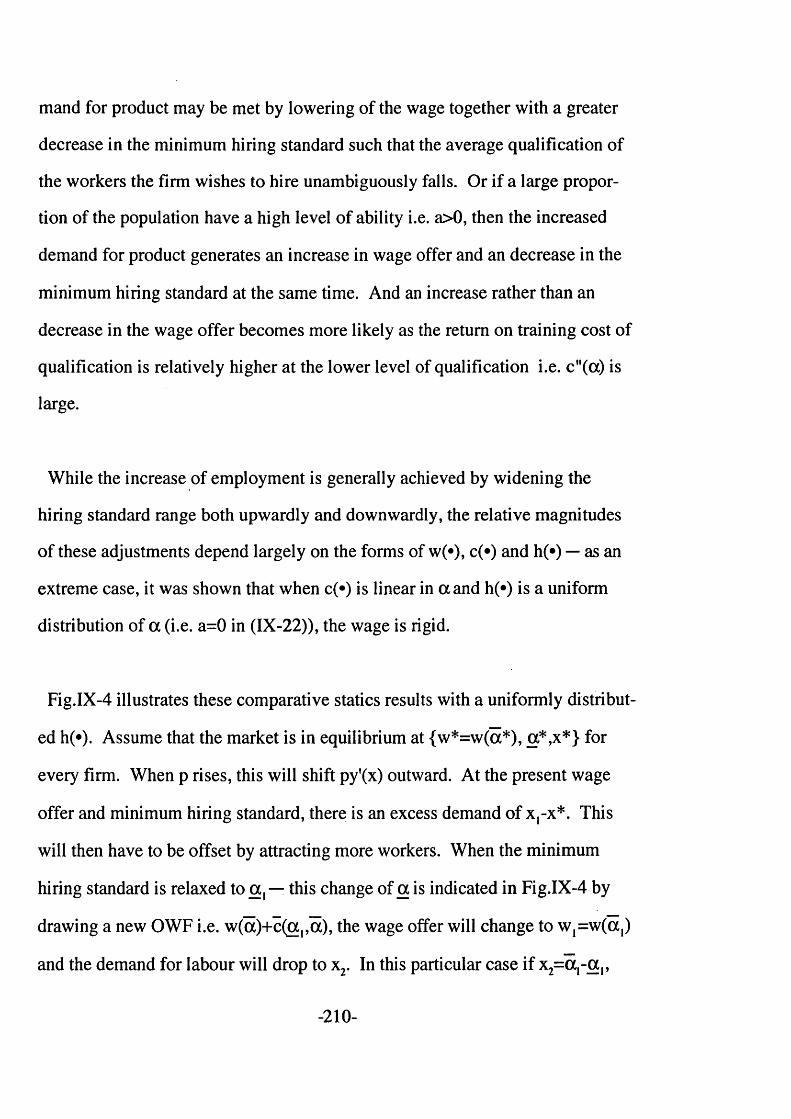
mand for product may be met by lowering of the wage together with a greater
decrease in the minimum hiring standard such that the average qualification of
the workers the firm wishes to hire unambiguously falls. Or if a large propor
tion of the population have a high level of ability i.e. a>0, then the increased
demand for product generates an increase in wage offer and an decrease in the
minimum hiring standard at the same time. And an increase rather than an
decrease in the wage offer becomes more likely as the return on training cost of
qualification is relatively higher at the lower level of qualification i.e. c"(a) is
large.
While the increase of employment is generally achieved by widening the
hiring standard range both upwardly and downwardly, the relative magnitudes
of these adjustments depend largely on the forms of w(«), c(«) and h(») — as an
extreme case, it was shown that when c(«) is linear in a and h(*) is a uniform
distribution of a (i.e. a=0 in (IX-22)), the wage is rigid.
Fig.IX-4 illustrates these comparative statics results with a uniformly distribut
ed h(*). Assume that the market is in equilibrium at (w*=w(oc*), a*,x*} for
every firm. When p rises, this will shift py'(x) outward. At the present wage
offer and minimum hiring standard, there is an excess demand of x,-x*. This
will then have to be offset by attracting more workers. When the minimum
hiring standard is relaxed to a , — this change of a is indicated in Fig.IX-4 by
drawing a new OWF i.e. w (a)+c(a,,a), the wage offer will change to w,=w(a,)
and the demand for labour will drop to x2. In this particular case if x2= a ,-a ,,
-210-

then the new equilibrium is reached. Note, however, that whether a*^(<)0
depends on c 2l>(<)0.
The main difference between these results and those obtained in the earlier
model is the existence o f the wage rigidity when the product demand changes.
In the present model, the wage rigidity occurs when c ( v ) takes a certain form,
e.g. linear. Then there are two ways to explain the wage rigidity within this
framework. One is to say that the wage rigidity occurs as an equilibrium phe
nomenon as in the earlier model. But for this, the characteristics o f c ( v ) has to
be specified. Namely, we need to assume a constant marginal return to qual
ification, with the return being defined by reducing the cost o f OJT. Another
way is to assume that the wage rigidity is a constraint imposed on the labour
market operation. With this approach it is easier to explain why the wage is
rigid
w.(a)
x* w* 0 a, a* a* a, aX X, x 2
Fig.IX-4
-211-

downwards only — namely, the pressure to keep the wage rigid only exists
downwardly. The result is a greater rise in the minimum hiring standard than
otherwise, which hits the low ability group harder.
(4) Policy implications
Firstly, when a uniform wage is offered to heterogeneous workers there is
always an incentive coming from workers as well as from firms to make the
workers distinguishable, even if the uniform wage system is to continue. Then
the government will do well by helping to reveal everyone's ability. Not to
make the information available to firms is to miss out a Pareto improvement i.e.
this will not help the workers either, although on the equity criterion this might
not appear to be desirable. The equal opportunity, however, should be given to
every worker in acquiring education before they come to the labour market.
Secondly, the excess supply in the labour market can not be eliminated by
advising the firms to reduce the wage offer — the firms simply would not do it.
One of the effective ways to eliminate this involuntary unemployment is to offer
some employment subsidy to the firms who are willing to lower their minimum
hiring standard.
Thirdly, as for the downward wage rigidity, it may not be desirable but this
inability of the wage to respond to the fall in demand for product can be com
-212-
plemented by a greater rise in the minimum hiring standard, with the result that
the low qualification workers are hit harder than when the wage is flexible. In
other words, the downward wage rigidity simply protects the more able workers
by sacrificing the less able workers. Hence allowing the downward wage
rigidity is not only inefficient but also unequalizing, or socially undesirable.
Therefore the government should discourage any move towards the wage rigidi
ty*
In this chapter we have established the following;
Firstly, it was pointed out that in the real world observationally distinguishable
workers may be paid uniformly, despite the neo-classical claim that they ought
to receive different wages. Rather the distinguishability determines not the
wage of each worker but the ability range of workers to be employed at that
unique wage. This was supported by a Japanese example of a university grad
uate recruitment process. Thus the model is particularly relevant to the labour
market for new recruits who require training , and not for already skilled work
ers.
Secondly, the main difference between the model of this chapter and the model
of the earlier chapter is the treatment of the minimum hiring standard — the
earlier model can be thought of as a special case of the present model with the
minimum hiring standard constrained at zero. Also it is worthwhile noting that
at the equilibrium demand is always equal to supply, the latter being defined as
-213-

the number of workers bounded between the wage offer and the minimum
hiring standard.
Thirdly, an increase in product demand will always be met by lowering of
minimum hiring standard, while the response of the wage offer is not determi
nate. With a certain specification of functions, it was claimed that the wage
would react positively to the change in demand unless the population is concen
trated at low qualification, in which case a negative response by the wage to the
change of product demand is possible. Also if the marginal return of education
in reducing the cost of OJT is much greater at a low level of qualification, then
this tends to cause the positive response of the wage to the change in product
demand.
Finally, the policy implications are: (1) the government should encourage the
information on the individual ability to be available to firms. (2) to eliminate
the excess supply of labour the government should encourage the firms to
employ the workers with low qualification by offering, for example, some
employment subsidy to firms willing to employ them. (3) the government
should bear in mind the distributional effect of allowing the downward rigidity
of wage and should discourage any move towards it.
-214-

CHAPTER X : CONCLUSION
This work has offered an alternative approach to the theory of wage determina
tion, producing new and interesting interpretations to labour market phenomena.
The following are the summary of the work and some suggestions for the future
research.
There have always been cynical criticisms against attempts by neo-classical
economists to explain theoretically the real world phenomena. And the labour
issues are probably one of the most "sacred” areas, to which the economists
with scientific rationality have found it difficult to enter, as some feel that such
an approach applied to labour market analysis is too simplistic to describe
complicated human mind and the institutions created by it. It makes it is dif
ficult to find 'the standard economic theory' for labour economics. In fact there
are many theories and ideas, be it neo-classical or otherwise, but none could be
considered as outstanding or prominent in this field of economics.
The theories, however, could be categorized into either an institutional type or
a neo-classical type. Consider the various approaches presented in the survey of
Chapter II. There is a trade-off between theoretical rigour and intuitive appeal
at one end of the spectrum there is the institutional approach, which offers
intuitively appealing and realistic explanations of the labour market phenomena
but seems to miss out theoretical rigour and at the other end there are various
-215-
types of the neo-classical approach, which seem to maintain the theoretical
rigour but have lost intuitive appeal. And these two types of approaches seem
to interact very little. Among those, however, the efficiency wage models and
the training models stand out closest as syntheses of the institutional approach
and the neo-classical approach, to bridge the gap between the theory and the
real world of labour market phenomena.
The present model shares the basic concept of adverse selection and invariably
contains the positive and negative features of the adverse selection models. For
example, the assumption of heterogeneous labour, which is the key assumption
of the adverse selection model, makes the model quite realistic, closing the gap
between the theory and the real world. This is a valuable attempt since one of
the most popular criticisms towards the neo-classical analysis of labour markets,
particularly from other social scientists, is that it is too simplistic to assume that
workers are homogeneous since the very formation of our society is based on
the diversity of the individual members of the society. However, when the
heterogeneity of labour is assumed together with the uniform wage, although in
the real world it is not unusual, it was necessary to justify theoretically that they
can co-exisf, as in Chapter IV.
In Chapter IV, a theoretically rigorous argument for the validity of uniform
wage was given, using the concept of informational equilibrium. It was shown
that the uniform wage assumption is a theoretically valid one within this model
when the monitoring cost is sufficiently high or when the ability distribution of
-216-

workers has relatively high density among the workers with high ability.
What the present model differs from the rest of the efficiency models and the
adverse selection models is the introduction of On-the-Job Training aspect of
labour. This concept of OJT as a part of labour market mechanism was also
suggested in Thurow(1975)'s institutional approach and thus the present model
is even more synthesizing than most of the efficiency wage models. Such a
modelling helps to correspond a type of labour market to an equilibrium type
and to its response to economic fluctuations. Throughout the chapters, c(*) acts
as a parameter for such a modelling. It is important to note that this approach
gives new insight and direction to the market analysis of heterogeneous labour.
While the efficiency wage models can suggest the existences of job queues and
rigid wages, our model can go further to determine the market characteristics of
such phenomena.
Chapter V extended the concept of training to include one more period in the
model. Based on the heterogeneous labour and multi-period the model explains
the existence of a job queue as well as the way the wage profile is upward-
sloping.
That the model has maintained the theoretical rigour can also be seen in Chap
ter VI. Using the Lagrangian multiplier method, it was pointed out that in the
world of heterogeneous labour, monopsony and competition are not always
distinct. One of the implications of this result is that to restrict monopsony in
-217-
the labour market does not always reduce the firms advantage relative to the
workers. It is hoped that the method be employed to investigate a more general
case of imperfect competition in comparison with perfect competition.
Chapter III and VII together form the main body of the present work. The
model offered explanations for the existence of unemployment and the down
ward rigidity as most of other adverse selection models do. The present model,
however, goes more than that to correspond the market characteristics to these
phenomena. Thus, for example, unemployment and thus downward wage
rigidity are more likely to occur in a skilled labour market. Based on these
analyses, it was suggested that the unemployment can not be eliminated by
lowering the wage — thus, for example, unemployment is not caused by an
unreasonably high minimum wage. It also suggested that policies to control the
demand side of the market such as accepting of immigration of able workers,
raising the educational standard of the domestic workers, or subsidizing the
firm’s OJT would be more effective.
Chapter VIII and Chapter IX have offered some new insights into the market
mechanism in general and of the labour market in particular. In Chapter VIII
the idea of multiple wage equilibrium in one market can offer a new dimension
to the analysis of income distribution. One important result here is that whatev
er happens in the society will first affect the weakest, to whom therefore the
policy makers need to pay greater attention. This is a rather cynical but perhaps
quite realistic view of the world. The derivation of a skewed distribution of
-218-

wage offers yet one more explanation to the Pigou paradox and further insight
into the trade-off between efficiency and equity. The further investigation into
this issue requires more time and space and thus it should also be left for other
occasion.
The model of Chapter IX is probably the closest to the real world mechanism
of labour market among the models presented in this work. But this means at
the same time that it is least theoretically rigorous. The minimum hiring stan
dard as one of the conditions for an employment offer is a realistic assumption
but to model this together with a uniform wage offer, although there is nothing
unusual in reality, requires some theoretical justification. As for the results
obtained here, the minimum hiring standard adjustment to the demand fluctu
ation when the wage is not flexible gives a new explanation to the wage rigidity,
It is worthwhile pointing out that this explanation allows both economic (in that
it assumes equilibrium) and non-economic (in that it allows downward wage
rigidity as a result of social agreement) aspects of labour market.
Its implication that involuntary unemployment exists among less qualified
workers says again that the weaker members of the society are more prone to
exogeneous shocks. However, this result slightly differs from the result in
Chapter IX — while in Chapter VIII the selection of the weaker is made at
random under excess supply as the workers are indistinguishable, in Chapter IX
the weaker are the low ability workers always. This sounds quite gloomy but
perhaps seems more realistic, and gives the true picture of what is going on
-219-

about who is actually hit the hardest.
Finally it needs to be mentioned that the real world of labour is much more
complex than what any of these models suggests. However, it has shown at
least that modelling of training and heterogeneous labour improves intuitive
appeal of the analysis greatly. And it is hoped that more investigations are
going to be made along this line of research.
-220-
BIBLIOGRAPHY
Abe, Y.(1994). “Specific Capital, Adverse Selection, and Turnover: A
Comparison of the United States and Japan”, Journal of the Japanese and
International Economies; 8(3), pp.272-292.
Acemoglu, D.(1997). “Training and Innovation in an Imperfect Labour Mar
ket,” Review of Economic Studies, 64, pp.445-464.
Addison, J. & Siebert, S.(1979). The Market for Labor, Los Angeles: Good
year.
Akerlof, G.( 1970) “The Market for 'Lemons’ : Quality Uncertainty and the
Market Mechanism,” Quarterly Journal of Economics, 84(3), pp.488-500.
(1976).“The Economics of Caste and of the Rat Race and Other Woeful
Tales,” Quarterly Journal of Economics, 90(4), pp.599-617.
(1982).“Labour Contracts as Partial Gift Exchange,” Quarterly Journal
of Economics, 97(4), pp.543-569.
(1984).“Gift Exchange and Efficiency-wage Theory: Four Views,”
American Economic Review, 74(2), pp-79-83.
& Yellen, J.(1986). “Introduction" in Akerlof, G.A. & Yellen, J. (ed.):
Efficiency Wage Models of the Labour Market, Cambridge University
Press.
Altonji, J. & Spletzer, J.(1991). “Worker Characteristics, Job Characteristics,
and the Receipt of On-the-Job Training”, Industrial and Labor Relations
Review; 45(1), pp.58-79.
-221-

Arrow, K.(1973). “Higher Education as a Filter,” Journal of Public Economics,
2, pp. 193-216
Ashenfelter, O. & Card, D. (1985). “Using the Longitudinal Structure of Earn
ings to Estimate the Effect of Training Program,” Review of Economics
and Statistics, November, pp.648-660.
Azariadis, C.(1975).“Implicit contract and underemployment equilibria,”
Journal of Political Economy, 83(6), pp.l 183-1202.
Bhagwati, J. & Srinivasan, T.(1977).“Education in a 'Job Ladder1 Model and
the Faimess-in-hiring Rule,” Journal of Public Economics, 7, pp. 1-22.
Baily, M.N.(1974).“Wages and Employment under Uncertain Demand,”
Review of Economic Studies, 41(1), pp.37-50.
Barro, R. & Grossman, S.(1971).“A General Disequilibrium Model of Income
and Employment,” American Economic Review, 60(1), pp.82-93.
Barron, J., Black, D. & Loewenstein, M.(1989). “Job Matching and On-the-Job
Training”, Journal of Labor Economics; 7(1), pp. 1-19.
Bartel, A.(1992). “Training, Wage Growth and Job Performance: Evidence
from a Company Database,” NBER Working Paper No.4027, March.
Becker, G.(1964). Human Capital; A Theoretical and Empirical Analysis with
Special Reference to Education, National Bureau of Economic Research.
& Stigler, G.(1974). “Law Enforcement, Malfeasance and the
Compensation of Enforcers”, Journal of Legal Studies, 3, pp. 1-18.
Booth, A.(1991). “Job-related Formal Training: Who Receives It and What Is It
Worth?” Oxford Bulletin of Economics and Statistics, 53(3), pp.281-
294.
-222-

& Satchell, S.(1994). “Apprenticeships and Job Tenure,” Oxford Eco
nomic Papers, 46, pp.676-695.
Bosworth, D., Wilson, R. & Assefa, A.(1993). “The Market for Training: A
Human Capital Approach”, International Journal of Manpower; 14(2-3),
pp.33-46.
Bowles, S.(1981).“Competitive Wage Determination and Involuntary Unem
ployment : A Conflict Model,” mimeo., University of Massachusetts.
(1983).“The Production Process in a Competitive Economy: Walrasian,
Neo-Hobbesian and Marxian Models,” mimeo., University of Massachu
setts.
Cain, G.( 1976).“The Challenge of Segmented Labour Market Theories to
Orthodox Theories: A Survey,” Journal of Economic Literature, 14,
pp.1215-1258
Calvo, G.(1979).“Quasi-Walrasian Theories of Unemployment,” American
Economic Review, Proceedings, 69, pp. 102-107.
Carmichael, L. & MacLeod, B.(1993). “Multiskilling, Technical Change and
the Japanese Firm”, Economic Journal; 103(416), pp. 142-160.
Chapman, P.(1993). The Economics of Training, LSE Handbooks in Economics
Series, Harvester Wheatsheaf.
Clemenz, G.(1986).“The Impact of Imperfect Monitoring on the Efficiency
Wage Hypothesis,” Empirica, 13(2), pp.203-219.
Clower, R.(1965).“The Keynesian Counter-Revolution: A Theoretical Apprais
al,” in Hahn, F. & Brechling, F.(ed.): The Theory of Interest Rates,
London.
-223-
Dixit, A.(1990).“Optimization in Economic Theory,” Oxford University Press.
Donaldson, D. & Eaton, C.(1976). “Firm-specific human capital: a shared
investment or optimal entrapment?”, Canadian Journal of Economics,
Vol.9, no.3, pp462-472.
Doeringer, P. & Piore, M.(1971). Internal Labour Markets and Manpower Anal
ysis, Heath Lexington Books.
Eaton, C. & White, W.(1982). “Agent Compensation and the Limits of
Bonding”, Economic Inquiry; 20(3), pp.330-343.
Elias, P.(1994). “Job-related Training, Trade Union Membership, and Labour
Mobility: A Longitudinal Study,” Oxford Economic Papers, 46, pp.563-
578.
Elliot, R.(1990). Labour Economics : A Comparative Text, Macgraw-Hill.
Fallon, P. & Verry, D.(1988). The Economics of Labour Market, Philip Allan.
Fields, G.(1974).“The Private Demand for Education in Relation to Labour
Market conditions in Less-developed Countries,” Economic Journal, 84,
pp.906-925.
Folli, L. & Harris, C.(1996). “Learning, Wage Dynamics, and Firm-Specific
Human Capital,” Journal of Political Economy, 104(4), pp.838-868.
Gibrat, R.(1931). Les inegalites'economiques, Paris, Sirey.
Champemowne, D.(1953).“A Model of Income Distribution,” Economic Jour
nal, 63, pp.318-351.
Greenhalgh, C. & Stewart, M. (1987). “The Effects and Determinants of Train
ing,” Oxford Bulletin of Economics and Statistics, 49(2), pp. 171-
190.
-224-

Greenwald, B.(1986). “Adverse Selection in the Labour Market”, Review of
Economic Studies; 53(3), pp.325-3pp.47.
Grossman, S. & Hart, O. (1983).“Implicit Contracts under Asymmetric
Information,” Quaterly Journal of Economics, Supplement, pp. 123-156.
Guasch, J. & Weiss, A.( 1980).“Wages as Sorting Mechanisms in Competitive
Markets with Asymmetric Information: A Theory of Testing,” Review of
Economic Studies, 47, pp.653-664.
& _____(1981).“Self-selection in the Labour Market, American
Economic Review, 71(3), pp.275-284.
& _____(1982).“An equilibrium analysis of wage-productivity gaps,”
Review of Economic Studies, 49, pp.485-497.
Hashimoto, M.(1979).“Bonus Payments, On-the-job Training and Lifetime
Employment in Japan,” Journal of Political Economy, 87(5), pp. 1086-
1104.
(1981).“Firm-Specific Human Capital as a Shared Investment,”
American Economic Review, vol.71,no.3, pp.475-482.
Ishikawa, T.(1981).“Dual Labour Market Hypothesis and Long-run Income
Distribution,” Journal of Development Economics, 9, pp. 1-30.
Jovanovic, B.(1979).“Job Matching and the Theory of Turnover,” Journal of
Political Economy, 87(5), pp.972-990.
Katz, L.(1986).“Efficiency Wage Theories: A Partial Evaluation" in Fisher, S.:
Macroeconomic Annual 1986, National Bureau of Economic Research,
pp.235-276.
& Ziderman, A.(1990). “Investment in General Training: The Role of
-225-

Information and Labour Mobility”, Economic Journal; 100(403),
pp.l 147-1158.
Kreps, D.(1990).“A Course in Microeconomic Theory,” Harvester Wheatsheaf.
Koike, K.(1991). S h igoto no K eiza igaku (Economics of Work) in Japanese,
Toyo Keizai Shinposha.
(1995). The Economics of Work in Japan, ( The English Version of
Koike, K.(1991)), LTCB International Library Selection No.3, LTCB
International Library Foundation/4
Kuznets, S.(1955).“Economic Growth and Income Inequality,” American
Economic Review, 45(1), pp. 1-28.
(1963).“Quantitative Aspects of the Economic Growth of Nations,”
Economic Development and Cultural Change, 11(2), pp. 1-80.
Lazear, E.(1979). “Why Is There Mandatory Retirement?”, Journal of Political
Economy; 87(6), pp.1261-1284.
& Rosen, S.(1981).“Rank-toumaments as Optimum labour con
tracts,” Journal of Political Economy, 89(5), pp.841-864.
Leibenstein, H.(1957). Economic Backwardness and Economic Development,
NY: Wiley.
Levhari, D & Weiss, Y.(1974).“The effect of Risk on the Investment in Hu
man Capital,” American Economic Review, 64(6), pp.950-963.
Levine, D.(1993). “Worth Waiting for? Delayed Compensation, Training, and
Turnover in the United States and Japan,” Journal of Labour Economics,
11(4), pp. 724-752.
Lucas, R.(1977). “Hedonic Wage Equations and Psychic Wages in the
-226-

Returns to Schooling,” American Economic Review, 67(4), pp.549-558.
Lynch, L.(1990). “Private Sector Training and the Earnings of Young Work
ers,” NBER Working Paper No.2060-88.
(1991). “The Role of Off-the-job vs. On-the-job Training for the Mobility
of Women Workers,” American Economic Review, 81(2), pp.151-
156.
Lydall, H.(1968). The Structure of Earnings, Oxford University Press
MacDonald, G.(1980).“Person-specific Information in the Labor Market,”
Journal of Political Economy, 88(3), pp.578-597.
(1982).“A Market Equilibrium Theory of Job Assignment and Sequen
tial Accumulation of Information,” American Economic Review, 72(5),
pp.1038-1055.
Malcomson, J.(1981).“Unemployment and the efficiency wage hypothesis,”
Economic Journal, 91(364), pp.848-866.
Manning, A.(1990).“Implicit-Contract Theory" in Sapsford, D &
Tzannatos,Z.(ed.): Current Issues in Labour Economics, MacMillan.
(1994).“Labour Markets with Company Wage Policies,” mimeo., Lon
don School of Economics.
Mincer, J.(1970).“The Distribution of Labour Incomes: A Survey with Special
Reference to the Human Capital Approach,” Journal of Economic Liter
ature, 8, pp. 1-26.
(1974). Schooling, Experience, and Earnings, National Bureau of Eco
nomic Research.
(1976).“Progress in Human Capital Analyses of the Distribution of
-227-
Earnings" in Atkinson,A.B.(ed.): The personal distribution of incomes,
George Allen & Unwin.
(1993).“JobTraining: Costs, Returns, and Wage Profiles,” in Studies in
Human Capital: Collected Essays of Jacob Mincer, vol.l, pp.263-281.
& Higuchi, Y.(1988). “Wage Structures and Labor Turnover in the
United States and Japan”, Journal of the Japanese and International
Economy; 2(2), pp.97-133.
Mirrlees, J.(1975).“A Pure Theory of Underdeveloped Economies,” in Rey
nolds, L.(ed.): Agriculture in Development Theory, New Haven: Yale
University Press.
Mookherjee, D.(1988).“In voluntary Unemployment and Worker Self
selection,” Journal of Economic Theory, 45, pp.171-188.
Moore, J.(1985).“Optimal Labour Contracts when Workers have a Variety of
Privately Observed Reservation Wages,” Review of Economic Studies,
LII, pp.37-67.
Mortensen, D.(1978).“Specific Capital and Labor Turnover,” Bell Journal of
Economics. 9(2), Autumn, pp.572-586.
Nickell, S.(1976). “Wage Structures And Quit Rates”, International Economic
Review, Vol. 17, no.l, pp. 191-203.
Ohashi, 1.(1983). “Wage Profiles, Layoffs, and Specific Training”, International
Economic Review, Vol.24, no.l, pp. 169-181.
Olson, L., White, H. & Shefrin, H.(1979) “Optimal Investment in Schooling
when Incomes are Risky,” Journal of Political Economy, 87(3), pp.522-
539.
-228-
Pareto, V.(1897). Cours d'economie politique, Lausanne: Rouge.
Patten, T.(1997). Pay : Employee Compensation and Incentive Plans, The Free
Press.
Pigou, A.(1932). The Economics of Welfare, Macmillan.
Polachek, S & Siebert, W.(1993). The Economics of Earnings, Cambridge
University Press.
Rasmusen, E.(1989). Games and Information-An Introduction to Game Theory,
Basil Blackwell.
Riley, J.(1979).“Testing the Educational Screening Hypothesis,” Journal of
Political Economy, 87(5), S227-S252.
Rosen, S.(1974).“Hedonic Prices and Implicit Markets: Product Differentiation
in Pure Competition,” Journal of Political Economy, 82(1), pp.34-55.
(1985).“Implicit Contracts: A Survey,” Journal of Economic Literature,
23, pp. 1144-11175.
Rothschild, M. & Stiglitz, J.(1976).“Equilibrium in Competitive Insurance
Markets: An Essay on Economics of Imperfect Information,” Quarterly
Journal of Economics, 90(4), pp.630-649.
Roy, A.(1950).“The Distribution of Earnings and of Individual Output,” Eco
nomic Journal, 60, pp.489-505.
Salop, J. & S.(1976).“Self-selection and Turnover in the Labour Market,”
Quarterly Journal of Economics, 90(4), pp. 1-48.
Salop, S.(1979).“A Model of the Natural Rate of Unemployment,” American
Economic Review, vol.69 no .l, pp. 117-125.
Sapsford, D & Tzannatos, Z.(1993). The Economics of the Labour Market,
-229-

Macmillan.
Sattinger, M.(1980). Capital and the Distribution of Labour Earnings, North-
Holland Publishing Company.
Shackleton, J.(1995). Training for employment in Western Europe and the
United States, Aldershot, U.K.
Shapiro, C. & Stiglitz, J.(1982).“Equilibrium Unemployment as a Worker
Discipline Device,” mimeo., Princeton University.
Shultz, T.(1965).“Personal Income Distribution Statistics of The United
States,” prepared for the Joint Economic Committee of Congress.
Smith, A.(1776) The Wealth on Nations ( reprinted in 1977 by Penguin Books)
Spence, M.(1973).“Job Market Signalling,” Quarterly Journal of Economics,
87(3), pp.355-374.
(1976).“Competition in Salaries, Credentials and Signaling Prerequisites
for Jobs,” Quarterly Journal of Economics, 90(1), pp.51-74.
(1981).“Signalling Screening and Information,” in Rosen, S.: Studies in
Labour Markets, National Bureau of Economic Research.
Starrett, D.(1976).“Social Institutions Imperfect Information and the Distribu
tion of Income,” Quarterly Journal of Economics, 90(2), pp.261-284.
Stevens, M.( 1994a). “A Theoretical Model of On-the-Job Training with
Imperfect Competition”, Oxford Economic Papers; 46(4), pp.537-562.
(1994b).“Transferable Training and Poaching Externalities,” mimeo,
Trinity College, Oxford University.
(1994c).“Labour Contracts and Efficiency in On-the-job Training,”
Economic Journal, 104(March), pp.408-419.
(1994d).“An Investment Model for the Supply of Training by Employ
ers,” Economic Journal, 104(May), pp.556-570.
Stigler, G.(1961).“The Economics of Information,” Journal of Political Econo
my, 69(3), pp.213-225.
Stiglitz, J.(1974).“Wage Determination and Unemployment in L.D.C.'s: The
Labour Turnover Model,” Quarterly Journal of Economics, 88(2),
pp. 194-227.
(1975).“Incentives, Risk and Information: Notes towards a Theory of
Hierarchy, Bell Journal of Economics, 6(2) Autumn, pp552-579.
(1975).“The Theory of 'Screening* Education and the Distribution of
Income, American Economic Review, 65(3), pp.283-300.
(1976).“The Efficiency Wage Hypothesis, Surplus Labour and the
Distribution of Income in L.D.C.s, Oxford Economic Paper, 28(2),
pp. 185-207.
(1986).“Theories of Wage Rigidity" in Butkiewicz,J., Koford,K. &
Miller, J.(ed.): Keynes' Economic Legacy. N.Y.Praeger.
(1987).“The Causes and Consequences of the Dependence of Quality
on Price, Journal of Economic Literature, 25, pp. 1-48.
& Weiss, A.(1981).“Credit Rationing in Markets with Imperfect
Information, American Economic Review, 71(3), pp.393-410.
& _____ (1994).“Sorting Out the Differences Between Screening &
Signaling Models,” in Bachrach, B.(ed.): Oxford Essays in Mathematical
Economics, Oxford University Press.
Takeuchi, Y.(1995). N ihon no m eritoku rasii ( in Japanese) or Japan’s Meritocra
-231-

cy, Tokyo University Press.
Topel, R.(1991). “Specific Capital, Mobility, and Wages: Wage Rise with Job
Seniority,” Journal of Political Economy, 99(1), pp.145-176.
Thurow, L.(1975). Generating Inequality, New York: Basic Books.
Tinbergen, J.(1951).“Some Remarks on the Distribution of Labour Incomes,”
International Economic Paper, 1, pp. 195-207.
(1956).“On the Theory of Income Distribution,” Weltwirt schaftliches
Archiev, 77, pp. 155-173.
Weiss, A.(1980).“Job Queues and Layoffs in Labour Market with Flexible
Wage,” Journal of Political Economy, 88(3). pp.526-538
(1991). Efficiency Wages : Models of Unemployment, Layoffs &
Wage Dispersion, Oxford University Press.
Yellen, J.(1984).“Efficiency Wage Models of Unemployment,” American
Economic Review, Proceedings, 74, pp.200-205.
-232-