a systematic approach to graphical methods in...

A SYSTEMATIC APPROACHTO GRAPHICAL METHODS

IN BIOMETRYM. TARTER and S. RAMAN

UNIVERSITY OF CALIFORNIA, BERKELEY

1. Introduction

This paper deals with certain new graphical techniques which may be of valuein exploratory biometry. In two senses, emphasis is placed upon the systemati-zation of graphical procedures. One, a new theoretical result is obtained whichgives conditions under which nonparametric histogram procedures of Parzen[11], Rosenblatt [13], Watson and Leadbetter [25], as well as others, can betreated as a special case of Fourier series methods of Cencov [2], Tarter andKronmal [8], [19], [22], and Watson [24]. Two, by utilizing alternative weightedFourier series, most hitherto considered graphical procedures such as the histo-gram, scatter diagram, and cumulative polygon are placed within a single com-putational framework. This systematization is shown to provide a researcherwith both a comprehensive as well as a statistically and computationally efficientapproach to graphical data analysis.

In Section 6 of this paper, an example of the graphical display of biomedicaldata is presented. The bivariate case, for example, generalizations of the scatterdiagram, is considered in detail and the biomedical variable pair, bone age andchronological age, is used to demonstrate the application of this new graphicalprocedure.

Before proceeding to the sections of this paper that deal with the systemati-zation and exemplification of graphical methods in biometry, it may be worth-while to offer a brief explanation concerning what we consider to be the particularrelevance of the new graphical procedures to biometry. By way of contrast, thefollowing quotation ([1], p. 1), provides a clear exposition of the purpose under-lying what might be called the old graphical procedures:"Time after time it happens that some ignorant or presumptuous member of a

committee or a board of directors will upset the carefully-thought-out plan ofa man who knows the facts, simply because the man with the facts cannotpresent his facts readily enough to overcome the opposition. It is often withimpotent exasperation that a person having the knowledge sees some fallacious

Research supported in part by small grant to faculty-Dr. M. Tarter General ResearchSupport Grant 5 SO1 RR5441-10.

199

200 SIXTH BERKELEY SYMPOSIUM: TARTER AND RAMAN

conclusion accepted, or some wrong policy adopted, just because known factscannot be marshalled and presented in such manner as to be effective."

This quotation clearly indicates that the primary function the older graphicalmethods were usually designed to fulfill was the summarization of informationonce this information had been obtained.

It is the contention of the authors that while the older methods emphasizedthe expository, the newer graphical methods place an emphasis on the exploratory.While it is certainly important for the biometrician or biostatistician to be ableto present his "conclusions," the process of reaching these conclusions wouldnow seem to be an equally important application of graphics.

Unquestionably, the major impetus leading to exploratory graphics has beenthe availability of high speed digital computation. In particular, recent develop-ments involving the transmission of digitized graphical information over voicegrade phone lines may substantially increase the potential for graphical presen-tation. Unlike the now fairly common IBM 2250 graphics configuration, whichusually requires cathode ray tube (CRT) display units to be located within onehundred feet of a large central computer, the new IMLAC and other terminalswill make interactive graphics economical for those with access only to a smallcomputer or to a distant time shared computer system.

Before providing details of several new biostatistical graphic methods, oneadditional comment should be made. In a context where a new and substantiallymore powerful means of implementation becomes available, it may be of valueto thoroughly reconsider traditional methods and the modes of thinking whichengendered them and were engendered by them. The histogram, fractile diagram,scatter diagram, and other graphical tools were devised to meet certain specificgoals and to cope with a narrow range of practical limitations. Today it is rarelynecessary to group continuous data as a preliminary to the computation ofsample moments (and then apply Sheppard's corrections). The construction ofthe traditional histogram based on the division of the range of the randomvariable into class intervals may be similarly reconsidered.

In the next section, the recent evolution of the histogram will be described.Fortunately, in this situation the methods which in our opinion are the mostsuitable for biostatistical graphics will be shown to include histogram proceduresas a special case. However, it may not always be true that an elaboration of aconventional procedure is the most suitable alternative when matched with newmeans of implementation. For example, in Section 4, where an alternative to thefractile diagram is considered briefly, and in Section 6 which primarily concernsalternatives to the scatter diagram, it appears that the traditional graphicalmethods may be supplanted or at least supplemented by substantially differentprocedures.

2. Nonparametric and series graphical procedures

In this section, the symbolic or mathematical substructure of certain newgraphical procedures will be presented. Following an heuristic introduction to

GRAPHICAL METHODS IN BIOMETRY 201

the generalized histogram, a nonparametric procedure, introduced in [13] andinvestigated in [11], [25], [22], and others, it will be shown that for most practi-cal purposes generalized histogram type nonparametric procedures can be treatedas special cases of the series procedures, investigated in [2], [8], [22], and [24],as well as Schwartz [14]. Although this identity between nonparametric andseries procedures was previously mentioned in [8], it was not explicitly presented,primarily because of the lack of a practical method for implementing this result.However, new procedures devised by Tarter and Fellner [18] have recently beenfound to make it practical and desirable to consider nonparametric proceduresfrom a series point of view.

The process of constructing a typical "old style" histogram can be consideredas consisting of two separate steps. In Step 1 (see Figure 1), the domain of

26.3 5

18.5 10

1 7.2 2- -- ,15-20-

11.6 25-18.3 30-

23.0 35

41.6 40-45-50-5560

FIGURE 1Step 1.

interest is divided into equally spaced class intervals and it is ascertained intowhich interval each data point is to be allocated. In Step 2 (see Figure 2), foreach data point Xi, j = 1, . . ., n, a rectangular block, with width equal to theclass interval length h and with height equal to (nh)-l is added to the pile ofblocks already piled within the class interval which contains Xi. It is apparentthat Step 1, which is the geometrical analog of moment computation using afrequency table of grouped data, is necessary only if hand rather than machinecalculation is used. It is more sensible and efficient to center the jth data pointat the exact value assumed by Xj. The resulting irregularly packed pile of blockscan be easily "compressed" numerically by even the smallest digital computer(see Figure 3).Once one revises Step 1, it is a simple matter to generalize Step 2 and consider

alternatives to the rectangular shape of the blocks or counters that compile thecontribution of the individual data points to the final graph of the densityestimator 7 (see Figure 4).


p~ I ri

15 20FIGURE 2Step 2.

At this point, it is advisable to switch from graphical to symbolic expression.Let f(x) represent the joint probability density function of the p dimensionalrandom variate colunm vectors {Xj}, j = 1, * * *, n, where the Xj will be assumedto be independent and identically distributed. Let k represent an arbitrarycolumn vector of integers or p-tuples and let N represent the set of all k. For afixed sample size n, a generalized histogram.A that is, nonparametric estimatorof f [13], can be expressed as

(1) ](z) = n jElAE8(X Xi).nj=1If Step 1 but not Step 2 is revised so that the rectangular shape of each counteris retained but the jth counter is centered at Xj, then

(2) n (Z) =I(Z)

Contribution Centered at the Data Point

FIGURE 3Improving Step 1.


Contribution Distributed Over the Entire Range

FIGuRE 4Improving Step 2.

where H is a p dimensional rectangular parallelopiped within space EP withdiagonal corners 1t(Xi, X2, ... , £p), where £k = h/2 for aR k and IH representsthe indicator function of H.We will now show that a broad class of nonparametric estimators can be

expressed as series estimators. The latter were introduced independently in [2],[8], [22], as well as [24]. This result is somewhat surprising since at least twoauthors, Schwartz [14] and Wegman [26], have stressed comparisons betweennonparametric and series estimators and, hence, given the impression that thereare fundamental mathematical and statistical differences between them. Theo-rem 1 tends to indicate that for almost all purposes, nonparametric and seriesestimators can be treated as being different forms of the same estimator. Thus,in our opinion, the choice between the two alternatives should be made solelyon the basis of computational criteria.THEOREM 1. Assume that we are interested in the estimation of the multivariate

density f over a finite subregion of the p dimensional Euclidean space. (Without lossof generality we will define the support off to be the hypercube

(3) U--{X:-i < X. < s = l, * * *, p},where X. is the sth component of X.) Assume that the p dimensional nonparametrickernel, as defined in expression (1) has a uniformly convergent Fourier expansionon the hypercube

(4) V = {X: -1 < X. < i, S = 1, P}of the form(5) 6,(X) - bk eXp {27rik'(X - R)},

kEIV

where R' = (- * * ,-q). Then at every point X of the support region of f, the"nonparametric" estimator.? defined by expression (1) is identical to the "series"estimator


(6) E f3kbkexp {27rik'(X -R%kEN

where

(7) f3k = I-IF_ exp {-27rik'(Xi - R)}.j=1

The proof of Theorem 1 is obtained through simple algebraic substitution andinterchange of the order of summation. It is, of course, not necessary to expanda about the point R. However, expansion about R helps to establish the identitybetween expression (7) and the definition of Dk given in [22]. (In the remainingsections of this paper we will use the earlier definition, that is, omit R and assumeV to be the usual unit hypercube.) It might also be noted that if the functionfis defined as(8) f(X) = fl~/n if X =Xi, j=1,*.*n,

(8) f(X) = {O/n otherwise,then the Fourier series associated with f is

(9) ](X) -E' f3k exp {27rik'(X - R)}kEN

and

(10) ](X) = fvA(Z) S.(X - Z) dZ,where the integral is taken in the Lebesgue-Stieltjes sense. Hence, f can beconsidered to be the convolution of f with 6,.Now define the Fourier coefficient of the density f as

(11) Bk = fV exp {-27rik'(X - R)}f(X) dXand the usual goodness of fit criterion [22], [25], mean integrated square error(MISE), as

(12) J = E If(X) - (X)I2 dX.

By simple algebraic manipulation as in [24] and [18], one finds that the MISEof nonparametric-series estimator 7 equals(13) J(f, f) = E, {n1lbk12(1 - IBk12) + 11 - bk12IBk12}.

kEN

Consequently, forf and 8 as defined in the statement of Theorem 1, the prob-lem of optimal choice of the "best" kernel a is identical to the problem of choiceof "best" weights, bk = bkPt, in expression (6). This problem has been consideredin [24] as well as [18] with the result that

(14) bt = 1 + (n - 1)lBkj 2

The estimation of bkPt is considered separately by Fellner and Tarter in [18],where an estimator

Pt n - 1(15) ~~~~~bkn -1 - (n - 1)I3k 12


is derived as an analog to the inclusion rule for the choice of bk = 0 or 1 investi-gated in [22].

3. Computational considerations

It is not usually feasible to directly apply the series estimator derived inTheorem 1. For biomedical and other applications, graphical procedures mustbe considered from computational as well as statistical points of view. Whileoptimum weights (14) are estimable from given data, it is impractical to computemore than a moderate number of these coefficients. On the other hand, the esti-mators considered in [22] result in a very simple inclusion rule, namely, includethe coefficient Bk if and only if

(16) jBkl >

which is the dichotomous analog of weight (14) or, in the usual situation whereBk is unknown, use

(17) lf3kl2 > 2 )

which is the dichotomous analog of weight (15).Furthermore, since the asymptotically optimal kernel is the Dirac a function

(see [24]), the above procedure approaches optimality, that is, the MISEapproaches zero as n approaches infinity. Investigations with real data byRaman [12] indicate that satisfactory results may be obtained by using theabove technique with sample size as low as 45 pairs of observations to estimatecertain bivariate distributions.

In contradistinction to series methods, the use of nonparametric estimates ofform (1) for graphical purposes requires that the entire file of data points beeither stored or reentered into the computer in order to graph ] at each specificvalue of x. Since the estimator Ak and the inclusion rule (17) are symmetricfunctions of the observations, there is no need to allocate memory space in thecomputer for the storage of data. On heuristic considerations, we propose as astopping rule the termination of the search for a subsequence of coefficients (inthe bivariate case) as soon as two consecutive coefficients become negligible in ahorizontal and vertical scan of the array of coefficients.

Since the inclusion rule is the same for Bk and B_k, it becomes necessary tocompute and store the real and imaginary parts of only half the total number ofcoefficients. This again results in saving of computer memory and time.To further optimize the running time, we test the coefficients by the inclusion

and stopping rule after reading each set of 100 data points. Since the observa-tions are assumed independent, these intermediate estimates are unbiased.However, to be conservative we perform the test with the final sample sizesubstituted for n in the right side of inequality (17).In a typical example with 1000 pairs of observations from a 50 per cent


mixture of Gaussian distributions, the computation of the Fourier coefficientstook about nine minutes on an IBM 1130. The computational advantage of themethod will be evident by noting that in the above situation, the first 100observations took three minutes, the second 100 took one and a half minutes,the third 100 took one minute, the fourth and the rest took half a minute each.Moreover, the economy of summarizing the characteristic density by the seriestechnique can be appreciated by noting that the number of coefficients neededin the above situation was only 23. Studies performed by Kronmal and Tarter[8] have shown that the number of parameters required in the univariate caseis less than fifteen for most distributions, sample sizes, and intervals of estimation.

Besides the advantage of series forms that is related to the condensation ofstatistical information into a relatively few estimators, one might note a secondclosely related computational property possessed by most series procedures and,in particular, by expression (6). The statistics S are symmetric functions of theobservations and, hence, can be computed iteratively.The utility of the iterative computation of fAk is best illustrated by the appli-

cation of univariate modifications of expression (6) to the problem of estimatinga cumulative distribution function. Consider that the process of graphing thesample cumulative is almost identical to the process of ranking the data points.This has led to investigations [8] and [21] which deal with the use of seriesestimators as replacements for the sample cumulative.

In the next section, a general result is derived for which a special case, relatedto estimation of the cumulative distribution function, has been considered byKronmal and Tarter [8]. It has been shown ([8], Section 7) that the same subsetof indices M, minimizes the MISE of estimator PM that minimizes the MISE ofdensity estimator fm. Specifically, in the notation of this paper, letting p = 1,and x- represent the sample mean, and defining density estimator JM and cumu-lative estimator PM, respectively, as

(18) JM(X) = 1 + X_ fAk exp {27rikx}kEM

and

(19) PM'(x) = ( + x - ) + E (27rik) lf3k exp {27rikx},kEm'

where 0 ¢ M or M', then if goodness of fit is measured in terms of MISE, theset M should equal the set M'. Note that one can treat the term

(20) E_ (27rik)-YA exp {27rikx}

of expression (19) as a special case of the general series estimator defined byexpression (6), where

(21) bk ={r(27ik)-1 if kEr M',(21) = l,o ~ ~~~otherwise.


4. Weighted series estimators of functions derived from the density

In Sections 4 and 5, the choice of specific predetermined sequences of bk willbe considered from the following two points of view. One, the researcher maywish to obtain an estimate of a distribution density which possesses certaindesirable mathematical or statistical properties. (Weights chosen for this pur-pose will be considered in Section 5.) For example, one may wish to constraina density estimator to be nonnegative. Two, the target of the estimation process,rather than the density itself, may be a function derived from the density. Forexample, as previously discussed, one may wish to estimate and graph thecumulative distribution function. In this section, we will consider approachesto the latter class of problems which may be desirable from both a computationaland statistical point of view.

It may be of value to distinguish between the previously described two classesof problems by examining the MISE criteria associated with estimates of thedensity as opposed to the MISE between a statistical construct derived from adensity and alternative estimates of this construct. If this latter construct canbe expressed as a weighted sum of the coefficients of the Fourier series expansionof the density, then the following result applies.THEOREM 2. Define

(22) g(x) - , bkBk exp {21rikX}kEN

and(23) d(x) - _ bkBk exp {27rik'x},

where {bk}, k E N, is a preselected sequence of complex valued constants, N, Bkand ak are as defined in Section 2, and M c N. Then the same set M minimizesthe MISE J(g, #) for all sequences {bk}.

PROOF. From Theorem 1 of [22], one finds that

(24) J(g, 0) = E Var (bkBk) + E - b'kBkI2.kEM kE(NnM)

Therefore, the error increment A4Jk due to adding a term ko c M (as defined inCorollary 2 [22]) equals(25) bk((Var Bk) - iBkI2).Theorem 2 follows from the observation that for all nonzero bk, the sign ofexpression (25) is identical to the sign of

(26) (Var Nk) - IBkJ2.It is easily seen that estimates of density derivatives can be obtained, for

which Theorem 2 applies. Also, consider the problem of estimating the function

(27) 9(x) = f(x) + C Of(x),Oix1


which may (at least in the univariate case) be of value in empirical Bayes in-vestigations (here xJ is the sth component of the vector x). To estimate g(x),one might choose estimator D(x) of expression (23) with(28) bk = 1 + 27riCk.,where k. is the sth component of p-tuple k. If MISE is chosen as the measureof fit of 0 to g, then Theorem 2 implies that M can be determined by means ofinclusion rule (17). Naturally, it is also possible to modify "Fenlner weights"(15) to obtain a more statistically efficient estimator of expression (27). Thedecision of whether to use an inclusion rule or a weighting procedure should, ofcourse, take into account computational as well as statistical properties of thealternative procedures.A function derived from the density, which differs substantially from the

integrals or derivatives of f, will be considered in the remainder of this section.Define g(X) (x) as a univariate special case of expression (22) with(29) bk = exp {2(irkX)2}.Consider the following special case of the Fourier coefficients Bk of density f,

(30) Bk = E pa exp {2k7rk4L - 2(7rko8)2}.8=1

If all values of g,. and o, are sufficiently small, then f closely approximates asuperposition of c Gaussian densities with component means equal to {Ms},s = 1, ... , c, component standard deviations equal to {v,,}, s = 1, *--, c,and mixing parameters {pa}, s = 1, ... , c. Moreover, assuming X < a. forall s, the function g(0)(x) closely approximates a superposition of Gaussian den-sities which differs from f(x) only in that the set of component variances equals(31) {(a28 _ 2}S = 1, I- C.

Thus, if f3k is obtained from independent and identically distributed data arisingfrom a superposition of c Gaussian densities, one can estimate g(l)(x) by sub-stituting the special case of bk given by expression (29) into expression (23) andthen determining the set M by means of inclusion rule (17).

It may be of interest to mention that a very slight modification of the methodof decomposing superpositions described above can be shown to be identical toa particular form of nonparametric density estimation procedure considered in[11] (see p. 1068) and elsewhere. From expression (5), one finds that

(32) bk = fS6(x) exp {-27rik'(x - R)} dx.

If one considers the univariate Gaussian kernel a (see [11], p. 1068), one findsthat bk of expression (32), that is, a constant times the Gaussian characteristicfunction evaluated at t = -27rk, is identical to expression (29) with X = ai(where a- is the standard deviation of the Gaussian kernel). Hence, the methodfor decomposing superpositions of distribution functions described in this sectionand considered from other points of view in [3], [4], [7], [9], [10], and [15] is


closely connected to the nonparametric method for estimating densities basedupon Gaussian kernels. In fact, asM approaches N the specific series estimator 0with bk given in expression (29), which is used to decompose superpositions ofGaussian densities, approaches the specific nonparametric estimator (1) with 6,,set equal to a complex Gaussian function with p = 0 and o- = Xi. Interestingly,this particular choice of 8 reduces the variances of superimposed Gaussian com-ponents while a choice of 8 with a real positive variance can be shown fromexpression (10) to cause the variance of the density estimate to be greater thanthat of the density which is estimated.Although functions of form g of expression (22) are of interest and of practical

value in biomedical investigations, the display of composite functions, especiallytransgenerations of f and F are probably of primary biomedical utility (at leastin the univariate case). Consider, for example, the ratio of f(x) to the survivalcurve 1 - F(x), that is, the hazard function or, in some applications, the agespecific death rate.

It would not be appropriate to give an extensive survey of composite graphicalfunctions here, and hence, the remaining sections of the paper will deal with adiscussion and examples of the use of 0 with various choices of bk for the purposeof estimating a multivariate density. However, before leaving the topic of com-posite functions and statistical constructs derived from the density, two generalcomments seem appropriate.

One, the inclusion rule given by Theorem 2 applies to derived functions g ofexpression (20). Composite functions such as the hazard, fractile [6], confidenceband [16], transformation selection [20], [17] functions may make use of com-binations of derived functions 0. However, there is no guarantee that the par-ticular choices of 0 which are optimal (even in the weak sense of inclusion rule(16)) for the purpose of estimating various choices of g singly will, when com-bined to form a composite estimate, be optimal.Two, the computational convenience of the various estimators, which can be

put into form 0, makes it feasible to try new and more complex composite func-tions. For example, Tarter and Kowalski [20] have found graphs of the function

(33) 0,1-1 P(XA(x)(where 0 and b represent the standard Gaussian and ? and P the estimatedunknown density and cumulative) to be superior in many instances to the usualfractile diagram for the purpose of selecting a transformation of data to nor-mality.

5. Series density estimators utilizing a predetermined sequence of weightsIn this section a hybrid form of density estimator will be taken up. Consider

the case where one is interested in density estimates that are constrained tosatisfy certain mathematical properties, for example, be nonnegative. Alter-


natively, suppose that one wishes to find a computationally convenient esti-mator that corresponds as closely as possible to a conventional statistical form,for example, a histogram that utilizes rectangular blocks. We will consider inthis section a hybrid or compromise technique that tends to retain certainof the above prespecified mathematical properties while it approaches the statis-tical and computational efficiency of the series estimators introduced in Section 2.

Consider a specific nonparametric estimator, or equivalently, a series estimatorO with coefficients bk chosen to satisfy some mathematical constraint. For ex-ample, let I be defined by expression (1) with An given by expression (2). Here

(34) 1. ~~~~~~sin'rk'h(34) bk = 7,k'hAlternatively, if one wishes to estimate a density f with an estimator I that isconstrained to be nonnegative one might, in the univariate case, choose coeffi-cients bk to be the Fejer weights

b {(1 k) if mkl<m(35) b

O elsewhere,where m is some predetermined constant. Fejer forms of series estimators areconsidered in the univariate case in [8] and in the multivariate case in [16].

This section deals with density estimators a of form (23) with predeterminedsequences of weights bk, for example, as given in expressions (34) or (35). Theo-rem 3 concerns the choice of an appropriate inclusion rule (choice of set M)for such density estimators.THEOREM 3. Let a be any prespecified kernel whose Fourier expansion (as-

sumed, as in Theorem 1, to converge in V) generates the weight sequence {bk}.Then the weighted series estimator 0 of form (21), chosen so that an index ko E Mif and only if2(36) n'llbk,12 < IBkI2(1 + n-1b1 2- 11 -bk-11),has at least as small a MISE as the nonparametric estimator obtained by substitutinga into expression (1).The proof of Theorem 3 follows directly from MISE expression (13). Note

that if we assume that 8 is a symmetric kernel, then the bk are all real and theabove inequality reduces to

(37) +k 2nIBkj2bk < 1+ (n - 1)jBkI2which is equivalent to

(38) bk < 2b°tPI(see expression (14)).An alternative interpretation of inclusion rule (37) can be obtained as follows.

Define 8oPt(z) by using the values of bkPt given in expression (14) as the coeffi-cients of the Fourier expansion of 6oPt(z) (see expression (5)). Consider that by


Parseval's theorem the integrated square error ISE between 5 and 5opt that is,J (a(z) - 5Ot(z))2 dz, equals E kEN (bk - bkPt)2. Hence, to minimize the ISE oneshould include index k in the set M if and only if (bk - bkPt)2 < (b, t)2, that is,if bk < 2bkPt, which is identical to inequality (38).

It is, of course, necessary to check whether estimate O, to which the aboveinclusion rule is applied, retains the mathematical properties of the nonpara-metric estimators based upon 5. However, empirical studies with prespecifiedsequences of bk, for example, Fejer weights (35), have tended to show thatguaranteed possession of "mathematical" property, for example, nonnegativity,can usually be purchased only with an unacceptable increase in MISE. Thus,the hybrid procedures considered in this section may offer a reasonable com-promise in certain applications.While the choice of prespecified Fejer weight sequence (35) in conjunction

with inclusion rule (38) appears to be a useful graphical method, we are not atall certain of the value of prespecified sequences of bk, as given by expressions(34) and (29), for the purpose of density estimation. Like most procedures whicharise from nonparametric estimator (1), the effective use of weights (34) and(29) depends on the estimation of at least one parameter, for weight (34) theclass interval length h and for weight (29) the kernel standard deviation X.Although it is, of course, possible to estimate the parameters of "prespecified"bk by fitting bk, considered as a function of h or X, to bspt, this seems to be a round-about way of handling the estimation problem. Hence, in the example whichwill be considered in the next section, estimation is implemented from the seriespoint of view, using the computational procedures described in Section 3.

6. Biomedical application

In this section, we consider a specific application of the computational methodsoutlined in Section 3, for estimating a bivariate density.The basic data used in these calculations were measurements of chronological

age and bone age of children included in the Child Development Studies (KaiserFoundation, Oakland, California). The children included were a 10 per centsample, stratified by sex, race, and height (classified as tall, medium, short).For purposes of illustration, we have included here the data for white males ofmedium height. The particular bone selected is hamate and the bone ages aredetermined by matching the X-ray picture of the child with the standardradiological atlas prepared by Gruelich and Pyle [5]. The values read in areclose to within three months of the actual bone age since the graduation of theatlas is in intervals of three months.The program computes the bivariate probability density nonparametrically

from the data, using the technique of Fourier approximation of multivariatedensities (see [22]). The x variable is the chronological age in months and they variable is the bone age in months. The lower and upper limits are obtained


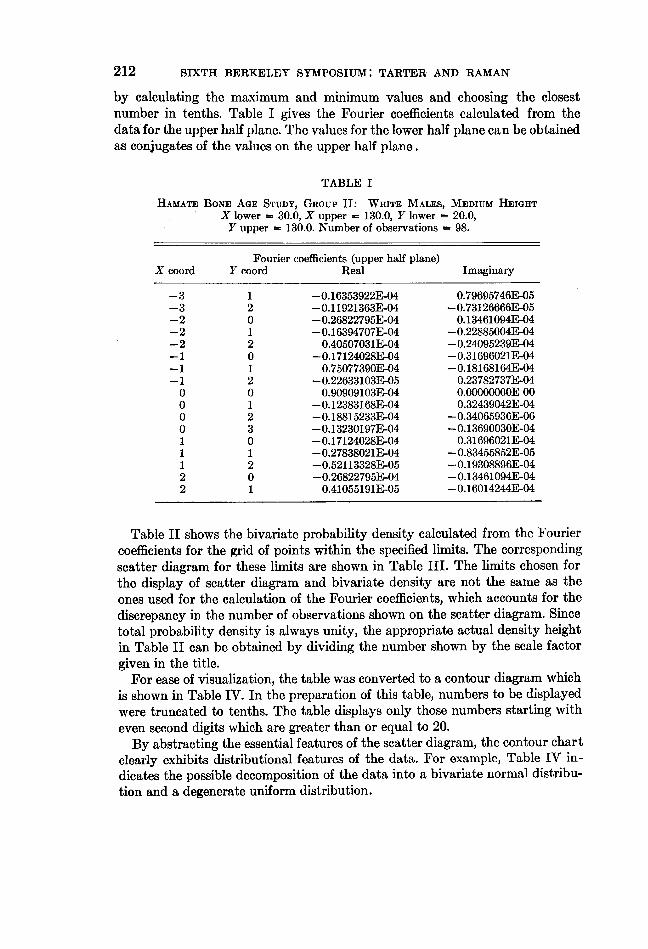
by calculating the maximum and minimum values and choosing the closestnumber in tenths. Table I gives the Fourier coefficients calculated from thedata for the upper half plane. The values for the lower half plane can be obtainedas conjugates of the values on the upper half plane.

TABLE I

HAMATE BONE AGE STUDY, GROUP II: WHITE MALES, MEDIUM HEIGHTX lower = 30.0, X upper = 130.0, Y lower = 20.0,Y upper = 130.0. Number of observations = 98.

Fourier coefficients (upper half plane)X coord Y coord Real Imaginary

-3 1 -0.16353922E-04 0.79695746E-05-3 2 -0.11921363E-04 -0.73126666E-05-2 0 -0.26822795E-04 0.13461094E-04-2 1 -0.16394707E-04 -0.22885004E-04-2 2 0.40507031E-04 -0.24095239E-04-1 0 -0.17124028E-04 -0.31696021E-04-1 1 0.75077390E-04 -0.18168164E-04-1 2 -0.22633103E-05 0.23782737E-040 0 0.90909103E-04 0.OOOOOOOOE 000 1 -0.12383168E-04 0.32439042E-040 2 -0.18815233E-04 -0.34065936E-060 3 -0.13230197E-04 -0.13690030E-041 0 -0.17124028E-04 0.31696021E-041 1 -0.27838021E-04 -0.83455852E-051 2 -0.52113328E-05 -0.19308896E-042 0 -0.26822795E-04 -0.13461094E-042 1 0.41055191E-05 -0.16014244E-04

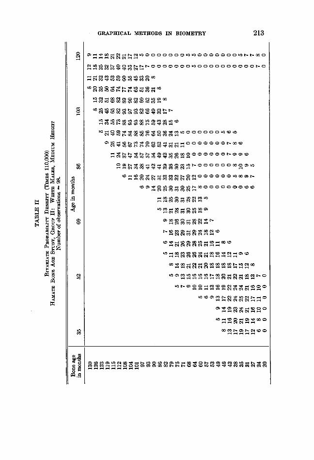
Table II shows the bivariate probability density calculated from the Fouriercoefficients for the grid of points within the specified limits. The correspondingscatter diagram for these limits are shown in Table III. The limits chosen forthe display of scatter diagram and bivariate density are not the same as theones used for the calculation of the Fourier coefficients, which accounts for thediscrepancy in the number of observations shown on the scatter diagram. Sincetotal probability density is always unity, the appropriate actual density heightin Table II can be obtained by dividing the number shown by the scale factorgiven in the title.For ease of visualization, the table was converted to a contour diagram which

is shown in Table IV. In the preparation of this table, numbers to be displayedwere truncated to tenths. The table displays only those numbers starting witheven second digits which are greater than or equal to 20.By abstracting the essential features of the scatter diagram, the contour chart

clearly exhibits distributional features of the data. For example, Table IV in-dicates the possible decomposition of the data into a bivariate normal distribu-tion and a degenerate uniform distribution.


0 co o 00 0000

eq v-o 0= ov

- -qcDO0c t-4C eeq -

-a eq co CO00 0 CO 000a.-C CO U4 10101 UCOe

00 0-40000ootcUnoo

10 Nq t0 q00 CCD 1 000 0_

CO 100000000 -t 000 CO k-I 00 U toCO 00COk-OOmOk- H

oo m v o cr m 4 Oo koCSd 0o+C 4oooooo DU

rA m co N t- 0 N 0 0 0 0 0 0 ulHl

on eqso0o)csonuCOoooooaa

°o m mN N N 1--

oo 10CO O>to o'"0100maoo

iX. O~C10t00 000k-10.0> 00000,-4

0 e

tSO~~~~e 41k 000k 1 COH~N eq.n

H~~~~~~~~~~~~~~~~~~~~I m cl cq-

k-COpo sLOCO000 00 >000

m~~~~~~~~~~~~~~szb o>c oo cc

A, 0 ~~~~~00 00a 000 0000t-

¢ Q HCO~COq,I,CO9C

0 0X O0O OOk-000000000

00 ¢OCO~COco q '-IM ' 0 N X

* 0-400'.~~~~~J4k--4CONcqOeqk-0e400o104~~~00 ~~ -4-4eqeqeqCOCOCO~~~-4COeqeq-4 4 O-400C

Lo10- 010kCo,4-0 0000CO 0000

cq M M XO-4N-eqCqCOCOCOt-,-

'-~ -4 q CO COeq eq

co

0 00000HNt-40LokNU:~~ ~ ~ ~ ~~~h -40 CO C'-00 Se -0:

C4 ~~ ~ ~ ~ ~ - -4------

214 SIXIH BERKELEY SYMPOSIUM: TARTER AND RAMAN

1-4 cl-4co -I -4 cq- 4

,- i4 co_

bo

-14

-4-4-4 CO _4

t.CO e -L

EH~~~~ co m- 00 _0t-t oC O-. 0 ' OM

H

r4=1

°~ ,.. I £tsNXeX>*


o ~~~eq °q °

0 0eq 00o oo o

0 0

0 00 0 0 0

0000oom~~~e ~o ~o o o

0^co00 00 co00~~~~~0~~~~~0 000ve

79 N 00~00 00 4co 4

00 0000 0

n~~~~e~ 000000 CO O

m co 0oagS; a a~~~~~~N NNOtO 000 000

0oo0

00 N .00 00.

N>N c e N eqC',

N N10 0

00 00

Nqe eq eq

eq eq e4 eq e

eq eq eq eq eq~~~~~cC414cqcl

X o neses~~~~~~^~~ooocnca C1oo o9ecouq ta o n s

0 00CD)000 ;. LO eq ~~~~~~~~~~~~~~~~~~eqeq4 eqe

pq Q~~~~~~~~~~~~~~~~~~~~~~~qe

00~~~~~~~~~~~~~~~~~~C

eqoco C0~q00kN -4t'N

0 ~ ~ ~~ ~ ~ ~ ~ ~ ~ ~ ~~~~0C


0 ,d - -

O k4 000CS1O CO 00 ftoN,1 -O

-4 ,-4

C o4 ,-4 CO CO C 0 N- -.4e--_ee -41-4-_

- CO k O 0 Cq CO a '-0oo Co-o_- -4 1-4 -4 i-I

o cq k oo o ci e- l0o oo C '-4

H COkO00O 00co

'-4 --

0 uto%o003wrs0000~00 O 4C -

i-4- to--

Qs n t~~CO b00 -00 NC7> 00 00 ei-0 _

tO 00000000 N>oO tC -

00 C~~1 CO ~4 C~~ N 000000001- COI3w..!on-~ s

C1 1O 00,iC CO NC

4 t. 0 O N C'm

3 to Nk0CO ~NC,4' -4 -4

o to

CO e 0I OmM + 0cCO OON ' C 0

a a -c-cooHooooomoocoAcoo¢ c -ec

000 C~~~ ~~4 N 000000 N ~~~~O '0'O ~~~4 CoC t-'-4'-' ~ ~ ~ -41- -

cmXO N W N~~C iON 000000 N- N N WO -.0 I-COz ~ ~ Nq -

-m ~ ootttc


Table V shows the empirical conditional probability distribution.(YiX) (ob-tained by dividing the bivariate probability density by the marginal density).

Also shown, in Table VI, are the estimated regression E(YIX), the standarddeviation, mode, median, and the two quartiles of I(YIX).

TABLE VI

ESTIMATED MODE, QUARTILES, MEDIAN, REGRESSION, CONDITIONAL STANDARDDEVIATION, VARIANCE, AND CORRECTION

X Mode Q(1) Q(3) Median E(YIX) S.D. V(YIX) Correction

35.0 34.6 31.7 36.8 34.3 35.0 6.1 38.20 038.4 34.6 31.6 42.9 33.6 35.7 6.9 47.79 241.8 34.6 31.5 42.2 33.3 36.1 7.2 52.19 545.2 34.5 30.0 44.2 37.8 43.4 20.7 432.55 148.6 38.3 34.7 55.1 47.4 49.3 21.7 473.22 052.0 38.3 39.6 59.0 50.6 49.3 14.8 220.58 255.4 64.0 41.9 62.2 51.2 53.9 14.2 202.41 158.8 63.9 49.3 66.2 60.2 58.8 13.0 171.01 062.2 67.7 56.5 71.1 63.4 63.8 9.9 99.70 -165.6 67.6 60.3 69.7 68.5 66.5 8.3 69.52 069.0 67.5 65.4 75.8 66.9 68.2 7.6 58.18 072.4 71.4 63.3 73.9 72.2 70.4 7.4 55.68 175.8 71.2 68.7 79.1 70.3 72.3 7.5 57.16 379.2 75.0 66.7 81.5 74.3 74.2 14.2 203.40 482.6 78.6 70.7 88.1 83.3 78.9 18.4 339.89 386.0 89.6 73.2 96.8 84.7 84.3 18.6 346.65 189.4 97.0 82.7 100.1 94.5 89.4 17.3 301.94 092.8 96.9 85.2 104.2 97.9 94.1 15.1 230.55 -196.2 100.6 89.2 109.1 102.4 97.4 13.8 190.81 -199.6 104.4 93.2 106.7 99.7 101.1 10.6 114.47 -1103.0 104.3 98.0 111.9 104.8 103.5 10.4 109.38 0106.4 104.2 95.7 110.1 102.8 105.6 10.1 102.50 0109.8 108.0 100.8 115.3 108.1 107.8 9.9 99.85 1113.2 107.9 105.9 113.6 106.2 109.9 9.6 93.53 3116.6 111.7 104.9 119.6 112.3 108.7 17.5 307.17 7120.0 111.6 101.4 119.7 113.3 98.2 32.1 1032.62 21

Biologically, for the average normal child the bone age should be the same asthe chronological age. In practice, however, there are sources of error due toobserver bias. Further, the atlas on which the assessments are based was cali-brated 40 years ago and, hence, the possibility of a secular trend on the osteo-logical maturation of California's children cannot be ruled out. Consequently, acorrection at each age to within three months can be obtained from the differenceof the chronological age and the regression estimate shown in the last columnof Table VI. After applying the correction to the original data, we then recom-puted the bivariate distribution. The corresponding results are shown in TablesVII, VIII, and IX. It can be seen from TableX that the second order correctionsare now negligible, at least at those levels where there are observations. Further,the contour chart after the correction shows a sharper segregation of the com-

218' SIXTH BERKELEY SYMPOSIUM: TARTER AND RAMAN

-4~ MMt

-44q q q-4-4

- -Cesoo000 'a4 0t- t-b00 C 1 4," 00N-4

4C eo 4t10 O 10M0 t-

SCO:)COtoSt=DtOo _

-40 C~ N N001_ie 400Nm Lo1 t- 00 0>m 00 to CO _1oCq 00100 to to N 0100-41 t

en~~ ~~o VD kllooN =oo ID0 O_C101tOO 0OOO

00001 04010

-40 Cq 101000000,-e e m4 00000000k'- 0

"ca410b40000000n0001oooooc0000

-4eq004~40000eqC 4c00 00000000a4c0coeqIcoq m oooobo

-4eqe11 000000eq ,CI -4-4

E-4 O.-0 -4~~~~~~4-C00000 q -S~~~~~~~~~~~~~~~

' 4

-X Q 00k 0000 N 00Unn

eqeq

t- Nleq 000-cc000 N ~t-4eq 0000 eqc

b~~~~~~~~~~~~~~~~~l moP co to 0 ko cc eq -4 -- 0

t- 100lw N 0O10 -4c 1~~eq0000eq eq cq c

N 0000 ° 001000 eq DONes m w

-4 4----4 4 --44-4

-4-4-4eqeq 4-4-4--4-4-4-4cq-4 -

eq p-40010~40 05_-4eqe0 n:10o 10 H°eoCwm OQUU eq eqs eq t lt

_4 eq eq cq cq _

to " w m t-~~~~crtoo>Numo -4 -4 ---4-4

10 oN -m0 D w 0 ~MM0 N 0 -0 N eq 100 -4-4-4---

0pqE


~~~ c~~~c

_l~~-~ -N-SC s_

P -N

00

~~~~~~~~~~ ~~~~~~~~cq,-

bLo

-o~~~~~~~~~~~~~~~~~~~~~~~~~~~~-

0 toco Locq o t m toN L -4 - Ct- - oN0 O t

z -~~c q0 m 0 - -t co -LOL -: -q 1

o

n H H H H ^ H~~~

a2~ ~~~~~~~~~~~- ccq~~

cY5 N _

0


0 0c-o eq q eq

eq co

o1 tot

00 00co

a00o 0000- ~~~~o00 00 w cie

E-4 ~~~~00 00 tJ4e

coooCoC

0 . 2~t s° oooot

o^>g~~~~~~~c to 0 oo

~00 Qe cq cq

cfNoS 0

;;~~~~~~~~~~~~~~c c c c°s"c°

to Cq Noesc°q0 0>>0>0>0

q 00 0 °

N 0-4 10 eqeq q

G>>Ho oq C1 C1 CI C sseett

0.00 c~~~~~~~~~~~~~~~~~~~~~~q eq eq e

Z ~~~~~~~~~~~~~~~~~D0000e eqqeqeq0000eq eq4 eq eq

eq4 eq eq

CV3

0 w c m l cq o I-m (ocoN0toco= eq 2g td) c , Q C 00 -t - c OL l lNC


TABLE X

ESTIMATED MODE, QUARTILES, MEDIAN, REGRESSION, CONDITIONAL STANDARDDEVIATION, VARIANCE, AND CORRECTION

X Mode Q(1) Q(3) Median E(YIX) S.D. V(YIX) Correction

35.0 34.6 31.4 36.6 34.0 35.2 6.1 37.78 038.4 34.6 31.6 42.9 33.6 35.7 6.9 47.71 241.8 34.6 31.5 41.8 33.2 39.2 18.9 359.02 245.2 34.6 31.2 40.2 39.6 40.8 20.3 414.60 448.6 34.5 36.1 58.1 42.3 46.6 20.3 415.92 152.0 38.3 33.7 65.7 44.9 48.7 15.6 244.81 355.4 67.7 36.5 67.9 51.2 53.8 15.9 253.14 158.8 67.6 49.3 72.3 59.0 59.4 13.7 187.86 062.2 67.6 55.3 70.3 62.3 64.7 9.9 98.65 -265.6 67.6 59.6 76.7 68.0 67.0 8.2 67.57 -169.0 67.5 65.3 75.8 66.9 68.3 7.5 57.15 072.4 71.4 63.7 74.7 72.9 69.6 7.0 49.84 275.8 71.3 62.1 80.1 71.2 71.4 7.5 56.62 479.2 75.0 68.1 77.3 76.4 72.1 12.4 154.25 782.6 74.9 72.7 84.8 79.1 76.7 16.4 271.27 586.0 82.3 75.2 98.4 86.9 82.9 18.2 334.86 389.4 93.3 76.9 100.4 88.1 88.6 17.4 304.33 092.8 96.9 85.9 104.0 98.0 93.9 15.4 237.68 -196.2 100.6 88.7 108.5 101.9 98.2 13.2 175.87 -299.6 104.3 92.6 106.2 99.2 101.6 10.7 114.89 -2

103.0 104.3 97.4 111.4 104.2 104.1 10.4 108.39 -1106.4 108.0 102.4 117.0 109.6 106.1 10.0 100.14 0109.8 107.9 100.3 115.1 107.7 108.2 9.8 97.14 1113.2 107.9 105.7 113.6 113.4 109.9 9.5 90.45 3116.6 111.7 105.3 120.2 112.7 108.3 16.7 280.88 8120.0 111.7 100.6 120.7 106.3 101.0 27.3 748.79 18

ponents. Also, it will be noted that the quartiles after correction give a morereasonable range between the Po.26 and Po.75 quartiles.

> K K K KThe authors would like to thank Professor J. Yerushalmy for making avail-

able the data utilized in Section 6 and Dr. W. Feilner and Dr. R. Brand forsuggestions concerning statistical aspects of this paper.

REFERENCES

[1] W. C. BRINTON, Graphic Methods for Presenting Facts, New York, The EngineeringMagazine Company, 1917.

[2] N. N. CENCOV, "Evaluation of an unknown distribution density from observations,"Soviet Math. Dokl., Vol. 3 (1962), pp. 1559-1562.

[3] G. DOETSCH, "Zerlegung einer Function in Gauss'sche Fehlerkurven," Math. Z., Vol. 41(1936), pp. 283-318.

[4] J. GREGOR, "An algorithm for the decomposition of a distribution into Gaussian compo-nents," Biometrics, Vol. 25 (1969), pp. 79-93.


[5] W. W. GRUELICH and S. I. PYLE, Radiographic Atlas of Skeletal Development of the Handand Wrist, Stanford, Stanford University Press, 1966 (2nd ed.).

[6] A. HALD, Statistical Theory with Engineering Applications, New York, Wiley, 1952.[7] R. A. KRONMAL, "The estimation of probability densities," unpublished Ph.D. thesis,

Division of Biostatistics, University of California, Los Angeles, 1964.[8] R. A. KRONMAL and M. TARTER, "The estimation of probability densities and cumula-

tives by Fourier series methods," J. Amer. Statist. Assoc., Vol. 63 (1968), pp. 925-952.[9] P. MEDGYESsY, "The decomposition of compound probability distributions," Hungar.

Acad. Sci. Inst. Appl. Math., Vol. 2 (1953), pp. 165-177. (In Hungarian.)[10] , Decomposition of Superpositions of Distribution Functions, Budapest, Pub. House

of the Hungarian Academy of Sciences, 1961.[11] E. PARZEN, "On estimation of a probability density function and mode," Ann. Math.

Statist., Vol. 33 (1962), pp. 1065-1076.[12] S. RAMAN, "Contribution to the theory of Fourier estimation of multivariate probability

density functions with application to data on bone age determinations," unpublishedPh.D. thesis, Department of Biostatistics, University of California, Berkeley, 1971.

[13] M. ROBENBLATT, "Remarks on some nonparametric estimates of a density function,"Ann. Math. Statist., Vol. 27 (1956), pp. 832-837.

[14] S. C. ScHwARTz, "Estimation of probability density by an orthogonal series," Ann. Math.Statist., Vol. 38 (1967), pp. 1961-1965.

[15] D. F. STANAT, "Nonsupervised pattern recognition through the decomposition of proba-bility functions," Technical Report, University of Michigan, Sensory Intelligence Labo-ratory, 1966.

[16] M. TARTER, "Variance and covariance formulas for evaluations of estimated orthogonalexpansions," to appear.

[17] , "Inverse cumulative approximation and applications," Biometrika, Vol.55 (1968),pp. 29-42.

[18] M. TARTER and W. FELLNER, "Some new results concerning density estimates based onFourier series," Proceedings of the Fifth Conference on the Interface Between Statistics andComputation, North Hollywood, Western Periodicals, 1972.

[19] M. TARTER, R. HOLCOMB, and R. A. KRONMAL. "A description of new computer methodsfor estimating the population density," Proc. Assoc. for Computing Machinery, Vol. 22(1967), pp. 511-519.

[20] M. TARTER and C. J. KoWALSKI, "A new test for, and class of transformations to,normality," Technometrics, Vol. 50 (1972), in press.

[21] M. TARTER and R. A. KRONMAL, "Estimation of the cumulative by Fourier series methodsand application to the insertion problem," Proc. Assoc. for Computing Machinery, Vol.23 (1968), pp. 491-497.

[22] , "On multivariate density estimates based on orthogonal expansions," Ann. Math.Statist., Vol. 41 (1970), pp. 718-722.

[23] J. VAN RYZIN, "Bayes risk consistency of classification procedures using density estima-tion," Sankhya Ser. A, Vol. 28 (1966), pp. 261-270.

[24] G. S. WATSON, "Density estimation by orthogonal series," Ann. Math. Statist., Vol. 40(1969), pp. 1496-1498.

[25] G. S. WATSON and M. R. LEADBETTER, "On the estimation of the probability density, I,"Ann. Math. Statist., Vol. 34 (1963), pp. 480-491.

[26] E. J. WEGMAN, "Nonparametric probability density estimation," University of NorthCarolina at Chapel Hill, Institute of Statistics Mimeo Series, No. 638, 1969.

a systematic approach to graphical methods in...

Documents