graphical methods and regression - sascommunity
TRANSCRIPT

Graphical methods and regression diagnostics
by
Thore Langeland, Statoil.
Paper presented at SEUGI, London, 1983.
ABSTRACT
A data set analysed by several oil companies is reviewed by
applying recently developed regression diagnostics. Due to
differing opinions among the oil companies concerning the choice
of regression line, this problem is addressed first. The
linearity assumption of the response and the independent variable
is checked by smoothing the scatterplot using robust locally
weighted regression. After removing some data points, the
remaining data set is discussed in greater detail using a wide
variety of diagnostic techniques, such as plots of leverage
points, studentized residuals, partial regression, partial
residuals etc.
In this study we have found the SAS'program package to be an
extremely convenient tool and the complete analysis is performed
simply by use of the procedures PROC ~1ATRIX and PROC GPLOT.
I Introduction
Simple and multiple regression analysis are commonly used by oil
companies in the evaluation of the reservoirs. However, many of
the tailored software systems for the interpretation of data such
as log, core and fluid data, contain regression programs that
just print out overall summary statistics like regression
coefficients and their standard deviations, coefficient of
determination, F-values, etc. These statistics ~an present a
distorted and misleading picture if the data set contains
influential observations which fail to adhere to the assumptions
that usually accompany regression models. This point is very
well illustrated by Anscombe (1973) using four examples that all

have identical overall regression statistics, but where the
scatterplots show very different relationship between the two
variables.
In addition to presenting basic information about regression
statistics all programs ought to have a possibility to explore
the properties of the residuals and to check the influence of the
design points on the estimation of the regression parameters and
the prediction function. The procedure PROC REG in SAS certainly
satisfies all these requirements, and, moreover, it is easy and
very convenient to use.
For a long time there has been a discussion in the geosciences
(Mark and Church (1977) and references therein) concerning the
appropriate choice of regression line. One of the results of
this discussion is a confused oil industry using a wide variety
of regression lines. on the same problems. This is further
elaborated in Chapter 3.
The assumption of linear relationship between two variables
possible after some transformations is frequently used by
reservoir engineers. The assessment of this assumption is
greatly enhanced by smoothing the points in a scatterplot,
particularly if the y-values are widely scattered for the same
x-value or for x-values lying close to each other. A smoothing
method introduced by Cleveland (1979) is further discussed in
Chapter 4.
To a large extent the data analysis in the oil companies is
oriented towards graphical methods. Graphical displays are an
important statistical tool and they significantly improve the
communication between different disciplines evaluating the
properties of the reservoirs. Our experience is that the
information in regression diagnostics is more rapidly understood
by non-statisticians if scatterplots are used. In Chapter 5 many
examples of such plots are provided by applying PROX ~~TRIX and
PROC GPLOT.
2

2 The Data
The amount of oil in a reservoir can schematically be given by
the formula:
(2.1) OI IP = V . f' 0, (1 - S ), w
where V is the volume, f is the fraction of reservoir rocks, 0 is
the porosity and S is the water saturation. The volume V is w primarily estimated by use of seismic data, while the remaining
parameters are derived from wire1ine logs and core data.
In order to evaluate the water saturation S of sha1y sands using w Waxman-Smits equation, the cation exchange capacity per unit
total pore volume Q must be known. For all the reservoirs in v the Norwegian part of the North Sea the determination of Q is v obtained either on the basis of laboratory measurements on cores
or predicting Q (for well zones lacking cores) from empirical v
relationship of the form:
(2.2) 1n (Qv) = a + b 1n (0).
In Figure 1 we have presented a scatterp10t of the natural
logarithm of Q and the natural logarithm of the porosity. The v plot consists of 61 pairs of laboratory measurements on cores
from several wells from a field which we shall call field A. Due
to variation in the Q values for the same porosity value or for v
porosity values lying close to each other, it is not obvious that
there is a linear relationship between the two variables.
3 Choice of reqression line
There seems to be many ways of fitting a straight line to a set
of pairs of measurements. In the literature we can find
recommendation to put the line so that the sum of the squared
devi~tion between the line and the points parallel to the y-axis
is minimised (regression of y or x), the sum of the squared
deviation between the line and the points parallel to the x-axis
is minimised (regression of x on y), the sum of the squared
3

deviation between the line and the points orthogonal to the line
is minimised (first principal component), or the sum of the area
of the triangles between the regression line and the lines
through the points parallel to the axes is minimised (reduced
regression) .
In all these cases the regression line is passing through the
point (x, y) and if b is the slope, the intercept is given by
a = y - bi.
Thus, in the continuing discussion, we shall concentrate on
finding an expression for the slope.
If the purpose is estimating a linear relationship between the
two varianles which are observed with errors, Moran (1971) shows
that in the case of structural relation (error-in-variables
model), the maximum 17_kelihood estimator of the slope in the
normal case is given by
(3.1) b = ~ s (s -k s + ( (s -ks ) 2+ 4ks ) !2) xy yy xx yy xx xy
where s is the covariance between x and y, sand s the xy xx yy variances of x and y, respectively, and k a known parameter
between 0 and infinite. By different choice of k, all the
criteria described above can be obtained (Mark and Church
(1977)).
The scatterplot of the logarithm of Qv and the logarithm of
porosity with four regression lines are exhibited in Figure 2.
The regression lines are the regression of y on x, the regression
of x on y, reduced regression, and the average of the two first
ones. All these lines were used by different oil companies for
field A, and it turned out that the difference in extrapolating
the results for the complete field caused some million dollars in
value difference in the estimate of oil in place (OIIP).
However, in the case of prediction, it is well known that the
best (minimising the variance) predictor of y given the
4

information of x, is the conditional expectation of y given x.
So, even if there is a structural relationship between y and x,
the best estimator of this predictor is nothing but the
regression of y on x (Lindley (1947)).
In our example we are in the business of predicting the Qv-value
for the zones with no core data, thus we ought to use the
classical regression method.
4 Robust locally weighted regression
The assessment of the functional relationship between the
logarithm of Q and the logarithm of the porosity in Figure 1 is v rather difficult because of the large variation in the scattering
of the points. By using an appropriate interpolation method that
portray the location of the response given the value of the
independent variable; the visual information in plot will be
greatly enhanced. Such a smoothing procedure was introduced by.
Cleveland (1979) and he called it robust locally weighted
regression. The method is a combination of smoothing locally
across the x-es by fitting a low-degree polynomical (as has been
done in time series for decades) and of robustifying this fit
against deviant points using ideas from robust statistics. The
smoothed points are then plotted in the scatterplot by special
symbols or, as we have done to obtain greater discrimination with
the points of the scatterplot, joinina the successive points by
straight lines.
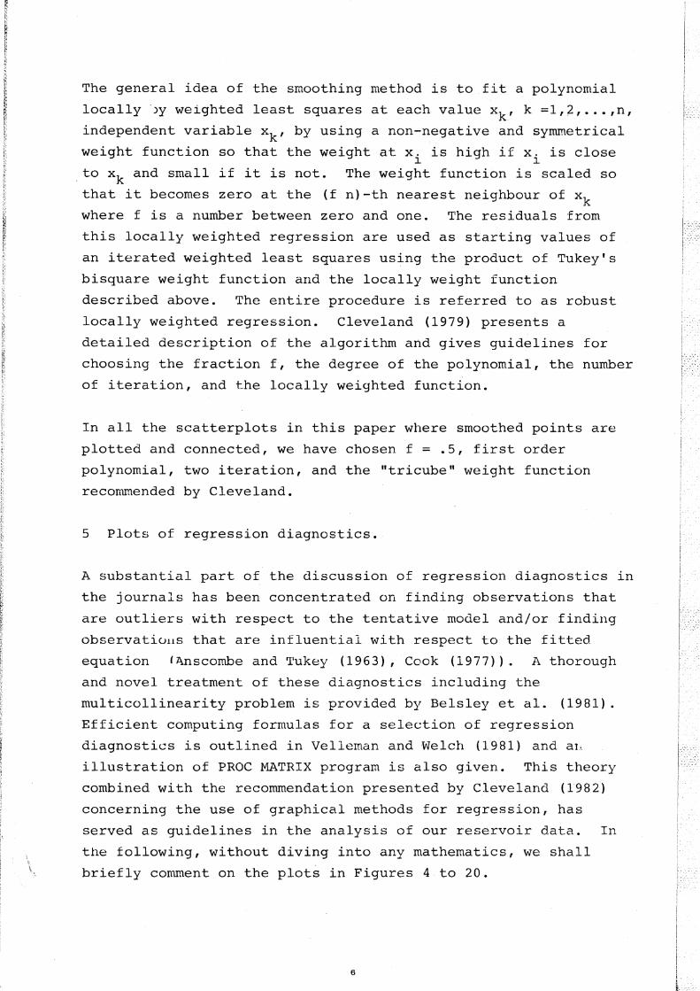
The result of applying Cleveland's procedure on the scatterplot
in Figure 1 is provided in Figure 3. Apparently the bulk of the
data fits reasonably well to the linear assumption of the
variables for porosity values less than (approximately) .24, but
at this point there is a shift in the regression line. The
porosity variations for these high values are probably goveined
by other factors than the variation in type and amount of clay in
the formation for which the Waxman-Smits model was built (Juhasz
(1981)). Mainly because of this argument we have deleted all
pairs of observations with porosity greater than .24 in the
discussion of the diagnostics in the next chapter.
5
I I I I l
1
The general idea of the smoothing method is to fit a polynomial
locallyly weighted least squares at each value x k ' k =1,2, ... ,n,
independent variable x k ' by using a non-negative and symmetrical
weight function so that the weight at x. is high if x. is close 1 1
.to x k and small if it is not. The weight function is scaled so
that it becomes zero at the (f n)-th nearest neighbour of x k where f is a number between zero and one. The residuals from
this locally weighted regression are used as starting values of
an iterated weighted least squares using the product of Tukey's
bisquare weight function and the locally weight function
described above. The entire procedure is referred to as robust
locally weighted regression. Cleveland (1979) presents a
detailed description of the algorithm and gives guidelines for
choosing the fraction f, the degree of the polynomial, the number
of iteration, and the locally weighted function.
In all the scatterplots in this paper where smoothed points are
plotted and connected, we have chosen f = .5, first order
polynomial, two iteration, and the "tricube" weight function
recommended by Cleveland.
5 Plots of regression diagnostics.
A substantial part of the discussion of regression diagnostics in
the journals has been concentrated on finding observations that
are outliers with respect to the tentative model and/or finding
observatiolls that are influential with respect to the fitted
equation (J\nscombe and 'I'ukey (1963), Cook (1977)). A thorough
and novel treatment of these diagnostics including the
multicollinearity problem is provided by Belsley et al. (1981).
Efficient computing formulas for a selection of regression
diagnostics is outlined in Velleman and Welch (1981) and aL
illustration of PROC MATRIX program is also given. This theory
combined with the recommendation presented by Cleveland (1982)
concerning the use of graphical methods for regression, has
served as guidelines in the analysis of our reservoir data. In
the following, without diving into any mathematics, we shall
briefly comment on the plots in Figures 4 to 20.
6

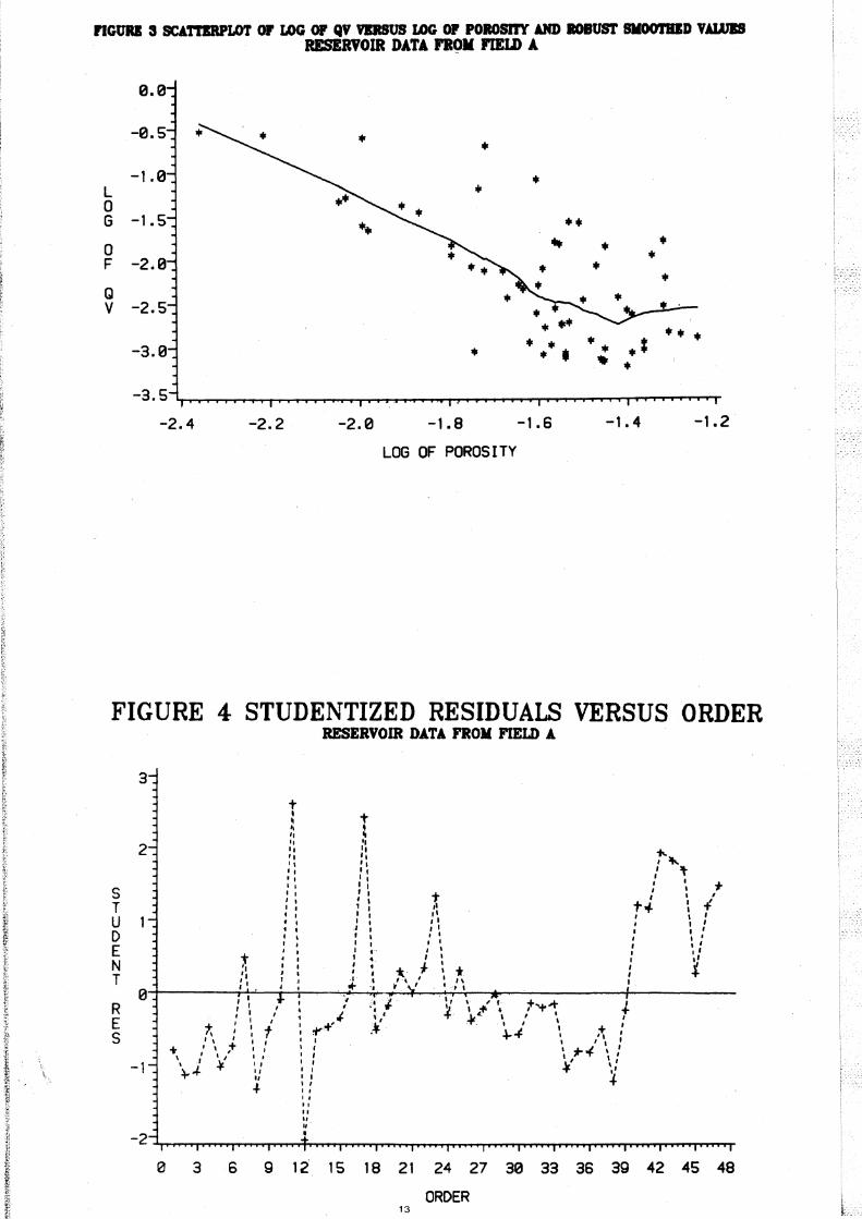
In search for lurking variables (Box (1966)) Joiner (1966)
advocates both forcefully and convincingly for plotting the raw
data and residuals with respect to time, order and spatial
arrangement. In Figure 4 the residuals are plotted versus
spatial arrangement (ordered by depth within each well). The
plot indicates some low frequency variation in the residuals.
However, the Durbin-Watson statistic is insignificant.
Furthermore, we note that observation numbers 11, 12, 17, 42, 43
and 44 contribute to the tails of the distribution of the
residuals and that more than 60 percent of the data are
negatively signed~
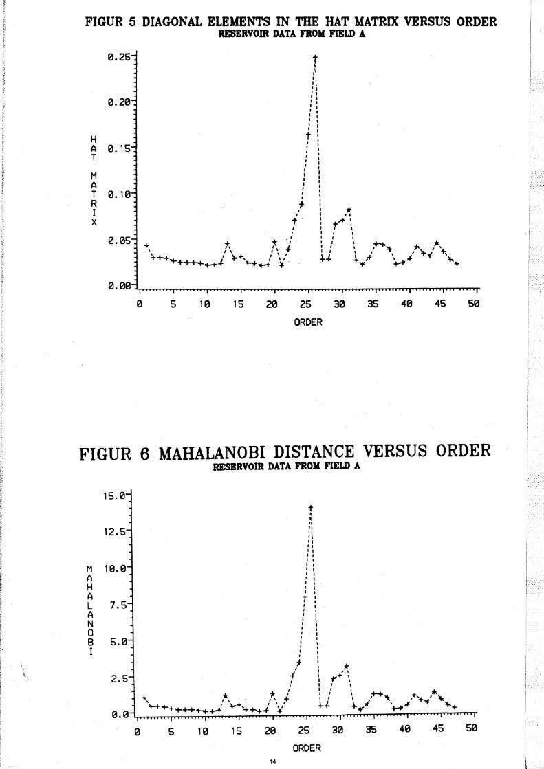
The leverage points h .. , i = 1,2, ••• ,n, which are the diagonal 11
elements of the hat matrix
(5.1)
where X is the design matrix, are plotted versus the spatial
ordering in Figure 5. Observations 24 and 25 call for special
attention according to the criteria developed by Huber (1981) and
Belsley et al. (1981). Hore or less the same information is
provided in Figure 6 by the l1ahalanobi's distance which for the
i-th data point, can be given as
(5.2) H. = (n-:-1) (h .. - lin), i = 1,2, ••• ,n. 1 11
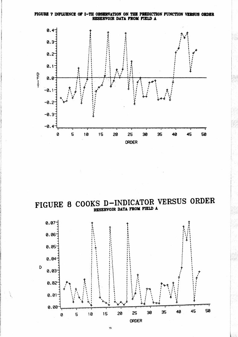
The next five figures, Figure 7 to 11, illustrate different
aspects of the combined effects of the residuals and the leverage
points. The effect of the i-th data point on prediction is
illustrated in Figure 7. The variable plotted is identical to
DFFITS in PROG REG (SAS User's Guide: Statistics) and all the
observations with large residuals plus observation number 23 are
influential on the estimation of the prediction function.
However, none of the calculated values are greater than the
size-adjusted cut off value (0.41) suggested by Belsley et al.
(1981). Cook's (1977) D-statistics is plotted in Figure 8, and
it is a standardized measure of the influence of the i-th data
point on the vector of the estimators regression coefficients:
The removal of any data point in the estimation does not move the
7

least square estimate to the edge of the 10% confidence region
for the regression coefficients based on the estimator for all
the observations.
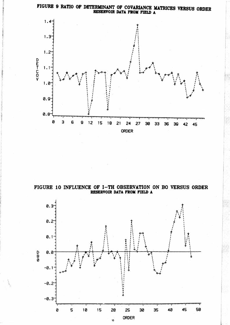
Another important aspect of regression is the covariance matrix
of the estimators of the regression cuefficients. In Figure 9 a
statistic identical to the COVRATIO in PROG REG is plotted and
the information gained by this plot is quite sioilar to the two
preceeding ones. Figures 10 and 11 plot the standardized changes
in the estimation of the coefficients using all observations and
deleting the i-th data point. The variables plotted correspond
to DFBETAS in PROG REG and observation numbers 23, 42, 43 and 44
are influential in these cases. As we might expect by now, even
by applying size-adjusted cut off value (.29) these observations
cannot be characterized as strongly influential.
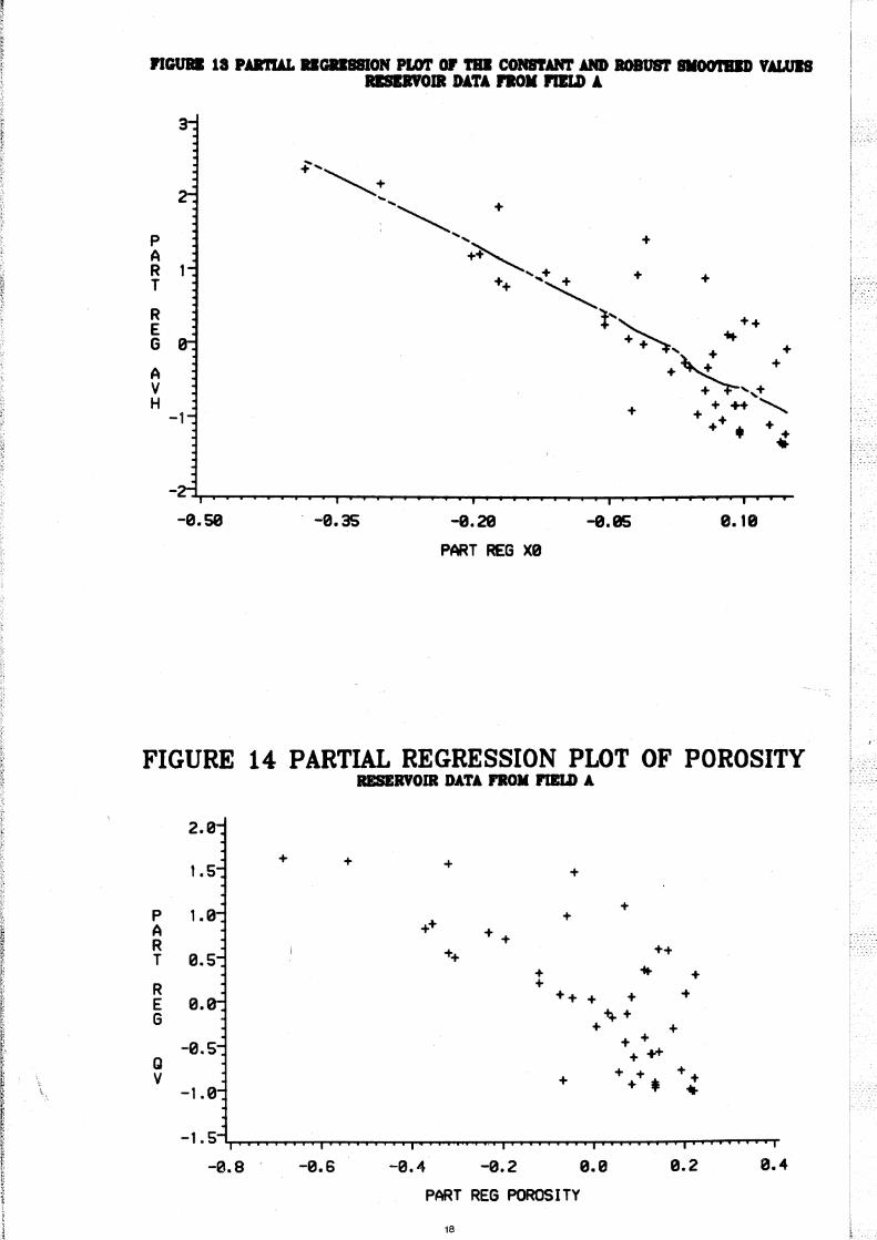
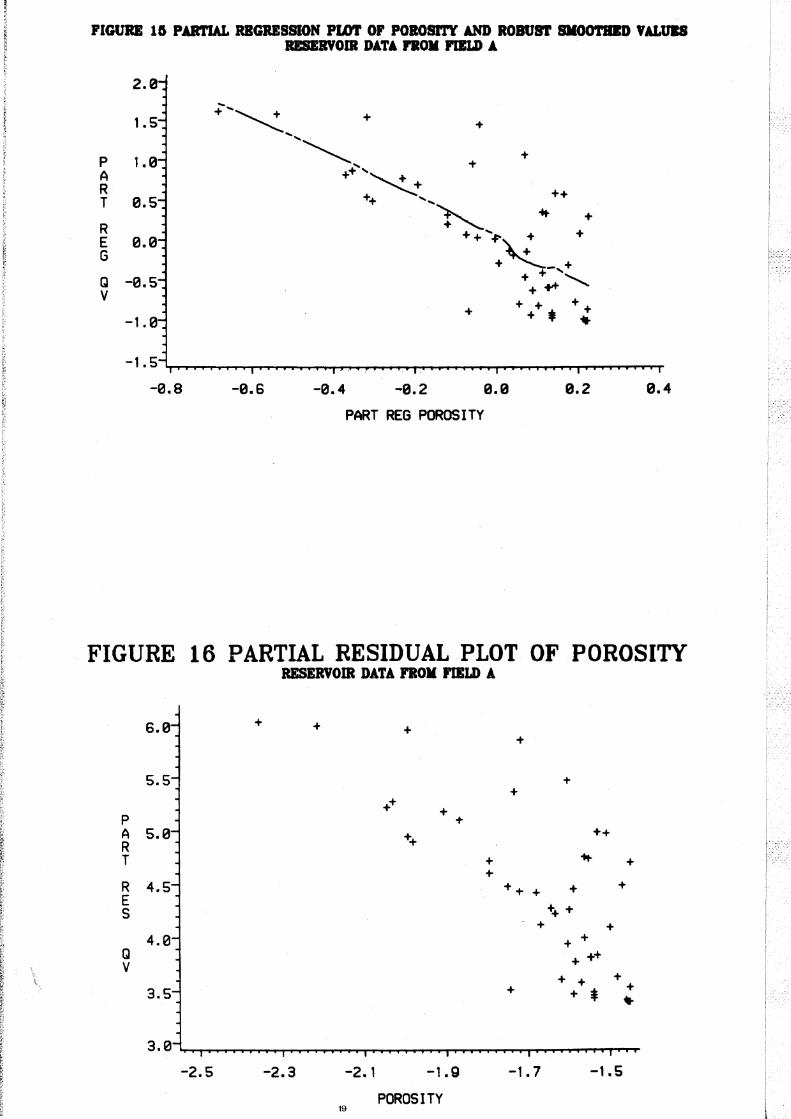
In Figures 12 to 17 we present the partial regression plot and
rhe partial residual plot (Velleman and Welch (1981)). The
visual interpretability is increased by smoothing the
scatterplots and using robust locally weighted regression. The
partial regression plot is good at explaining the effects of
collinearities and leverage points (but this requires a
possibility to identify the observations, which we look forward
to getting in SAS) while the partial residual plot is more
~ppropriate for diagnosing the non-linear relationship between
the response and the independent variables (Larsen and McCleary
(1972)). Nevertheless, these plots do support the tentative
model.
The normal plot of the residuals in Figure 18 indicates some
problems with the tentative model in (2.2). The empirical
distribution of the residuals are somewhat skewed to the right
and there is an unexplainable jump in the plot - hO residuals
between 0.2 and 1.0. The probability that none of the 48
residuals should not hit this interval, is .0000003 if they were
generated (independently) from a normal distribution with zero
mean and unit standard deviation.
8

Figure 19 shows that the scale of the residuals are leveling off
with increasing value of the response. This is to be expected
due to the sampling of the data.
The final plot is Figure 20, where we present the data and
assuming the model to be correct, the 95% confidence interval and
the 95% prediction interval.
6. Concluding remarks
The maiq purpose of this note has been to illustrate the
usefulness of displaying graphically some of the powerful
diagnostic techniques in regression analysis by applying the SAS
programe package.
We do not think that the set of reservoir data completely adhere
to the regression assumptions. However, the violations do not
seem to be major, so, for the time being, we have chosen to use
it as a working model.
9

REFERENCES
Anscombe, F.J. (1973):
"Graphs in statistical analysis,"
The American Statisticlan, 27, pp. 17-211
lmscombe, F. J. and J. ~v. Tukey (1963):
"The examination and analysis of residuals",
Technometrics, 5, pp. 141-160.
Belsley, D.A., E. Kuh, and R.E. Welsch (1980):
"Regression diagnostics,"
John Wiley & Sons, London,
Box, G. E . P . (1966):
"Use and abuse of regression,"
Technometrics, 8, pp. 625-629.
Cleveland, w.s. (1979):
"Robust locally weighted regression and
smoothing scatterplots,"
Journal of the American St:atistical Association, 74,
pp. 829-836.
Cleveland, W.S. (1982):
"A reader's guide to smoothing
scatterplots and graphical methods for regression,"
In Launer, R.L. and A.F. Siegel,
"Modern data analysis,"
Academic Press, London.
Cook, R.D. (1977):
"Detection of influential observation
in regression,"
Technometrics, 19, pp. 15-18.
Huber, P.J. (1981):
"Robust statistics,"
John Wiley & Sons, London.
10

Juhas z, I. (1981):
"Normalized Q The key to shaly sand evaluation using v the Waxman-Smits equation in the absence of core data
SPWLA 22nd Annual Logging Symposium.
Joiner, B. (1981):
"Lurking variables: Some examples,"
The American Statistician, 35, pp. 227-233.
Larsen, \l.A. and S.J. McCleary (1972):
"The use of partial residual plot in regression
analysis,"
Technometrics, 14, pp. 781-790.
Lindley, D.V. (1947):
"Regression lines and the linear functional
relationship,"
Journal of the Royal Statistical Society, Suppl., 9,
pp. 218-244.
Mark, D.M. and M. Church (1977):
"On the misuse of regression in earth science,"
Mathematical Geology, 9, pp. 63-75.
Moran, P.A.P. (1971):
"Estimating structural and functional
relationships,"
Journal of Multivariate Analysis, 1, pp. ·232-255.
SAS User's Guide:
Statistics
SAS Institute Inc.
Cary, North Carolina.
Velleman, P.F. and R.E. Welch (1981):
"Efficient computing of regression diagnostics,"
The American Statistician, 35, pp. 234-242.
11

FIGURE 1 SCAT1'ERPLOT OF LOG OF QV VERSUS LOG OF POROSITY RESERVOIR DATA FROII FIILD A·
-0.5 • • • • • • •• •
-1.5 • •• •• L
0 • ... • • G • • . '" . • • 0 ,.. F "' ....
•• • • Q -2.5 . '" •• '" V ... • ••
'" • • • ... • • •• • .. • -3.5
-2.4 -2.2 -2.0 -1.8 -l.S -1.4 -1.2
LOG OF POROSITY
rrcURB 2 SCA'I"l'DPLO'l' OF LOG QV VllSUS LOG or POROSITY AND roUR rnPiiiBNT CURYIFlTTING IJNIS RESERVOIR DATA FROM FIELD A
0
L ... o -1 ... G
•• 0 .... • ... F -2 ...
Q V
-3 •
-4
-2.5 -2.3 -2.1 -1.9 -1.7 -1.5 -1.3
LOG OF POROSITY
LEGEND: REF • ...... 1 --- 2 -- 3 4 ------- 5
Y WRT X=2 X WRT Y=3 RED REG=. AVE REG=5 12
"GUll 3 SCATl'lRPLOT or LOG or qv.9IRSVS JA)G or POROSITY' AND IOBUS1' SMOO'I'IIID VAWIS RISIRVOIR DATA nOli rJlLD A
0.0
-0.5
-1.0 L 0 G -1.5
0 F -2.0
Q V -2.5
-3.0
-3.5
-2.4
•
-2.2 -2.0 -1.8 -l.S
LOG OF POROSITY
• • .. -1.4
•••
-1.2
FIGURE 4 STUDENTIZED RESIDUALS VERSUS ORDER
S T U D E N T
R E S
3
2
0
1; • , I I I
+ , It ,
I I ,I
I I
-1 ~.4- -¥
t " I' , I
I
\ " , I
: t , , , . " " " ~
+ I ~ ~ I, " " " " " " " , ,
• I , , , , · , • • , , ,
RESERVOIR DA.TA FROM FIELD A.
t " I' 1'-,... : " It , : " * : t ' ' I
,,' to#- ~" ::~ I , ,
., , I : ~ :
i. !t ; :,1 '1. , I I I' " f I ;j :! ~, ~* : +
... 'J W ..... ' , .: \ ' .
'. & '" . \ ·1' * I • :: J.' I' I , ,. t"'+~ I
1'+,~;¥, f. k""\.i \, ;i;! I , I, I
f , '1--1- ' I , , , , ' : ~ \:
:: f ., •• " " " "
-2~~"T~~~~~~~'~~~~~~~~~~~~~~~~~~~~~~~~~~~ 3 S 9 12' 15 18 21 24 27 30 33 3S 39 42 45 48
ORDER 13
i
l~:,;:
{ f: ~ t ~ !, f
r l:
::
" ~: 1,
~ " ~:;
l r:; 5 f "(
, 1
FIGUR 5 DIAGONAL ELEMENTS IN THE HAT MATRIX VERSUS ORDER RESERVOIR DATA FROK nELD A
0.20
H A 0.15 T
M A T 0.10 R I X
0.05
o
t II II II II II II I, I I I I I I I I I ,
I I I I t, I I I I I I I t I I I I I I , , ,
f. , , ,
t' I I
I + ~, .
* , , +A \ I , I I I I
.' ~ t'+..... *' t-, ~ :\:. I +++ I ~+, ... \,' ..... +++;.++~ ++ .... +,' '
, "..... ~ I +. , J \,:f \ '-rtf. ' .,..,. .,." ~* !f,.+
5 10 15 20 25
ORDER
30 35 40 45 50
FIGUR 6 MAHALANOBI DISTANCE VERSUS ORDER
15.0
12.5
M 10.0 A H A L 7.5 A N a B 5.0 I
2.5
RESERVOIR DATA FROM FIELD A
t ~ q I, II II I, I, II I I I I , , , I I I I I , I I , ' I I I I
t : I I I I , I I \ I I , I I I I I I \. I I
,I I I I f I , \ *
f : +" I I 1" \ , I"
.... : :: '+-+ >k -ir r",", \ + I' \ , 'I;. '+"+' ~
',,--,-",- , "-+ ' \ , , J \" \~If 'of ..... + .-r -r-+ ..... +++............ ~ "+-+-+4- '+ .,..,..,... 'T'"T or
0.0~~~~~~~~~~~~~~~~~~~~~~~
o 5 10 15 20
14
25
ORDER
30 35 40 45 50
PleURB 7 INPWBNCI or I-TB OBSIRVATION ON TBB PllDICTlON FUNCTION VIISUI OlmJR RISIRVOIR DATA FlOI( FIILD A
t n " " 'I I " . I , ,
~ : : t : '. f :: , " I , ... ' ~ "
\ ' T .'
¥+ "'"
... • • • II .. " .. II II 'I I, , I I I I I • I , I I • , , , I I I I , , I
, t ,
.... ,+ I'T .. -1.1' , . I '., I .• :~. f
, ' I' I' ,I
" i
5 10 15
t t ~ : :' :: .' I, t' II .' " I J II I I I, , I I, , I I ,
: I ,
I ' I t I ' ,
I I ' , .. , '1 'I " , I 1: + ' ,I
" . ·'1 I' :' I , , , , ,
. I , \1 : ' "
.+. t. .... ' I • ~ I
.1 , . , • I
.J. : • I r
t I -¥ , I • , , I , ~ , , II
I " I I: : -'-, •
. , I I'. I t . : t· " I 1-' +... -+ , l' ': I' " · .J . .' I' •
I' • .' I
20
,., \.: ~ 1;: , . I, ' I , ,
:: -1-+ ' 'I, I' +*+ + !.
25
ORDER
as 40 45 50
FIGURE 8 COOKS D-INDICATOR VERSUS ORDER RESERVOIR DA.TA. FlOK FIlLD A.
0.07
0.06
0.05
0.04
D 0.03
0.02
0.01
0.00
o 5
t • 1\ 1 " ~ I , , , " . " I " I I' , I'
t :: , " • "' I I ,I
, ·1 • I I I , I' , , .
t , • q ~
" " II II
" II I, II II I I I I , ,
I , I
t t '1
I " 1\ :: I, " , \. I I U , , + :
I I , I , I I I I ,
., , ' · ,:" , ,,", • I I
: t I "
I I , ,
10
· . ' : ' . : ·1 I I , I I
I '~l .\ :' J' t I
I " I I I
-Ir : ~ I , I' I ........ , +. +. ~ "''If- +' '+'
15
15
: j t , I' ,
, 1\' .,. t I ~ : ~ I ~~ I' : , '........ I ,", II " r"T. , " " I
f " , " I I " \ ,'- • ,I \ I \I , , I • ~ ,I
.f. " ,I I' ~~ +-H. ""
25
ORDER
30 as 40
I r , , , , :t , , ,. , I I , ' " ,I ,I
~
45 50
, ~.
J~ ...
FIGURE 9 RATIO OF DETERMINANT OF COVARIANCE MATRICBS VERSUS ORDER RESERVOIR DATA FRO)( FIELD A
D E T C o V
1.4
1.3
1.2
1.1
1.0
0.9
+ • " " , . , , , ,
I , I , , ,
.,. : , , I , , , , , , , , , , ,
t : ,~ : ~ -;-1 \,
+ ,+, ~! I, ... • '........ . JI .... ,... r +-t + '" t. ~ ,., ... * +,', .J ,..... ',' .,"" T '.: "'tr, 1-;t', '!i 1\
\ , , ~, :I .. ~ \ I ,. " • \
+~ +' \,'; J ~: "" \ I' \ * : \ .f ,~ ... ' v ¥', I'., 4- I I • I T
I .• " ": I , , \
" ., • " ' 0\-" .. ' .,. ,.f ~ • , ' " '," ,'" " I ' ..... ' " .,' I + " , " I , "
, I J' " " ~ 0.8 ~~~~~~~~~~~~~~~~~~~~~~~~~~
o 3 6 9 12 15 18 21 24 27 30 33 36 39 42 45
ORDER
FIGURE 10 INFLUENCE OF I-TH OBSERVATION ON DO VERSUS ORDER RESERVOIR DATA FROII FIELD A.
D B o
0.3
0. 1
t " +. I I " , ,
I " I
" ~ : t ./. : ~ , I
t I' , · I' , t I", " " \ +-+ t: t : ! I ., " I, I, I r ' I I I. I , t ~ : \ :~: ~
": ~ ",·f' 'II ,
t I ., ""'+ ' + • , .f , ., I" \ ' ,
~--------~'~'--~~+---~-4'~-1r-~'+'~~+~'~I--~\~~-----4~--------r'----0.0 : \ ,'J' I ~' + \,' '.: ¥ ': +
-0.1
-0.2
-0.3
o
I It'" .1 . ..;. ¥ t I I I
+ ..:. " .!,f'" :, I I t' ;r " ., ., " '....,.
" \! V'~ : ': ~ I
: T +: l +, ,: +~ : ~
"
5 10 15 20
16
, , , , " II II , • ...
25
ORDER
30 35 40 45 50
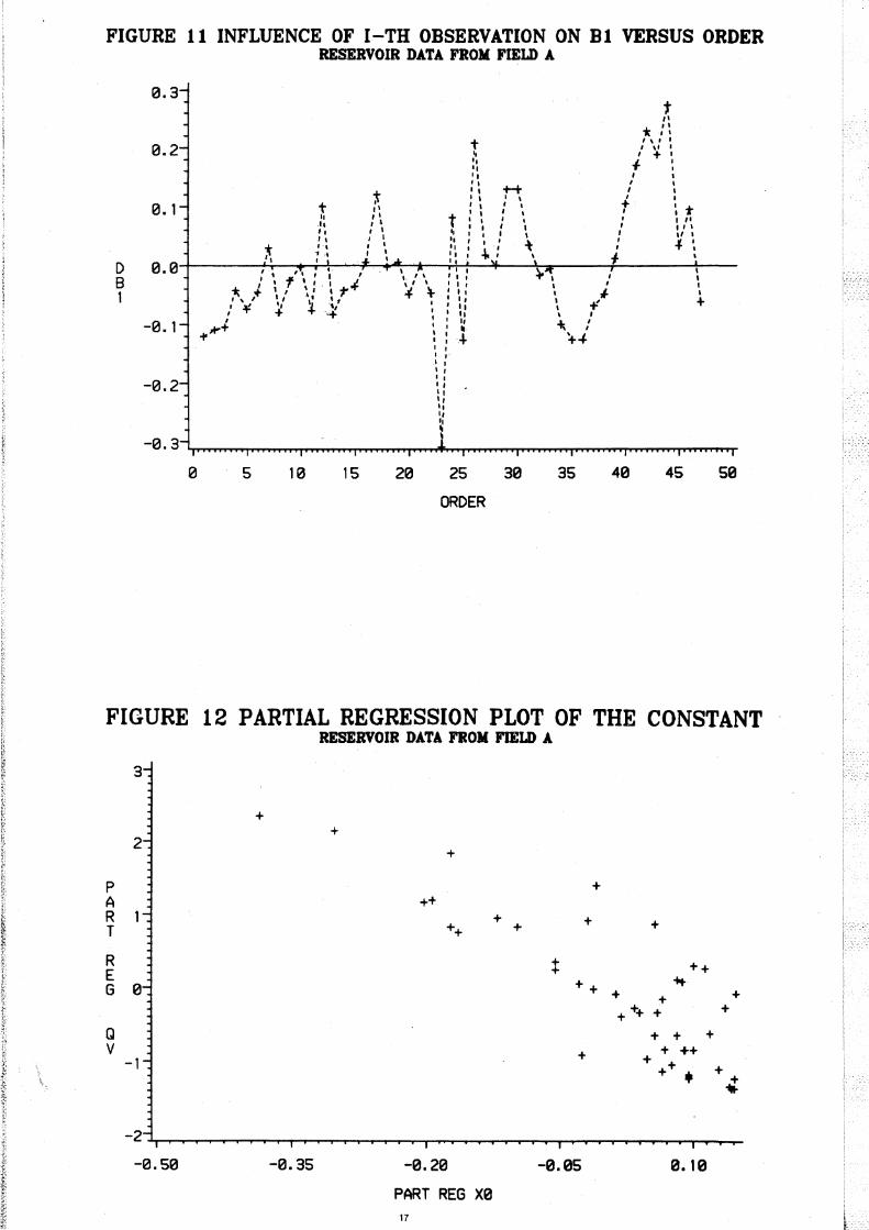
FIGURE 11 INFLUENCE OF I-TH OBSERVATION ON Bl VERSUS ORDER RESERVOIR DATA FROM FIELD A
D B 1
0.3 t " in
t : \: : ~ , + ' :: f :
0.2 II , ,
:~ +-I- : ~ t I, I \ .. I
t., : ~ : ~ ': t II : ~ t, ' , · I II :, , , L' , I '. , ,
I ~ ,I '. I' , I " , '" ,I :~ I' ___ :.f. ~
0. 1
~ : ;4 ,~ : ~ -" ': \ -I ' 0.0·~------~".--~,~.',~:.--~,~~~\-,~,--~,~:~~~--~+~,------T,--------~~----
i • f " • ~ \'" • " •
-0.1
-0.2
o
* + '.' ~: ~ r ~ + : I 'J. ' , ,,' " 'J .~,' I , I \ -tf + ,'.If .. .,. .• + • , " " , , , " ~ :
...... + : : J ++
5 10 15 20
, , , , . . 1, I, I, . , I. I, " ., " ,
25
ORDER
30 35 40 45 50
FIGURE 12 PARTIAL REGRESSION PLOT OF THE CONSTANT RESERVOIR DATA FROM FIELD A
3
+ +
2 +
P + A ++ R + + + T ++ +
R ::: ++ E ++ 'iot G 0 + + +
+ ++ + +
Q + + + v + + ++
-1 + ++ + + ~
-2
-0.50 -0.35 -0.20 -0.05 0.10
PART REG X0 17
i
~ ~ {.
~ ~ r.
I ~ ~, ~' \;
f :c t i
rlGUII 18 PAInUL BG8IS8ION PLOT or 'I'BI CONSTANT AND ROBUST SKOOTBID 'AWlS RlSllVOIR DATA noll nILD A
P A
2
R 1 T
R E G 0
A V H
-1
-0.50 -0.35 -0.20 -0.05 0.18
PART REG X0
FIGURE 14 PARTIAL REGRESSION PLOT OF POROSITY RESERVOIR DATA FROM FIILD A
2.0
+ + 1.5 + +
P 1.0 A R T 0.5
+ ++
+ + +
++ ++ + it +
R E 0.0 G
+ ++ + + +
~+ + +
-0.5 Q V
-1.0
+ + +++
+ + + ++ + , ... -1.5
-0.8 -0.S -0.4 -0.2 0.0 0.2 0.4
PART REG POROSITY
18
"CURB lG PARTW. RBGRlSSlON purr or POROSITY AND ROBUST SllOO'1'DU VALUII lBSIavOIR DATA F80II PIILD A
2.0
1.5
P 1.0 A R T 0.5
R E 0.0 G
Q -0.5 V
-1.0
-1.5
-0.8 -0.6 -0.4 -0.2 0.0 0.2 0.4
PART REG POROSITY
6.0 + + + +
5.5 + +
++ + P + A 5.0 ++ ++ R T + ill- +
+ R 4.5 ++ + + + E
++ + S + +
4.0 + + Q + ++ v
+ + + 3.5 + + *
+ .. 3.0
-2.5 -2.3 -2.1 -1.0 -1.7 -1.5
POROSITY 19

nGUllll ~ 'ALUI or ifG .. ,iiD IlllDUAJB UIIUI .... ,. 'ALUII AID .... ...".. 'AVJ.a RESERVOIR DATA FROII J'lELD A
A B S
S T U D E N
2.5
2.0
1.5
T 1.0
R E
+
+ +
+
+ + ~ +
t + --~
+
+
+
, " .... ~ +\V··~ .. _
+
S . ~ ++ + ++ + - ... ---------+ +
-2.8
o
L o -1 G
o F
-2 Q V
-3
+ +
-2.5
+ + + + ++
+
-2.4 -2.0
-
-2.3
+ + + -----
+ +
+ +
-l.S -1.2 -0.8
PREDICTED VALUE
-2.1 -1. 9 -1. 7 -1.5
LOG OF POROSITY 20
--t
-0.4
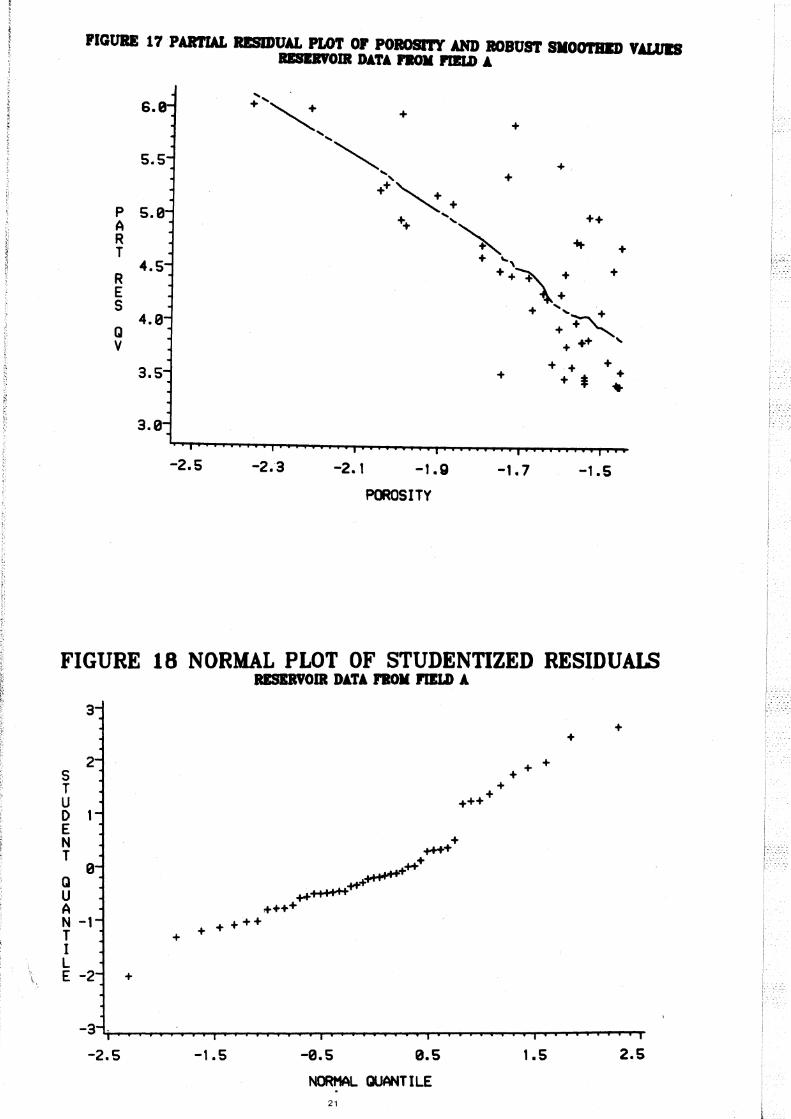
'IGURI 17PARTW. RlSWUAL PLOT or POROSITY AND ROBUST SIIOOTBID VAWIS ..... 018 DATA,.. PIILD A
P A R T
R E S
Q V
4.5
4.0
-2.5 -2.3 -2. t -1.9 -1.7 -1.5
POWSITY
FIGURE 18 NORMAL PLOT OF STUDENTIZED RESIDUALS IISIRVOIR DATA noll rJILD A
3 +
+
2 S T U D E N T
Q U A N -1
+ + T I L E -2 +
-3~~~~~r-________ ~ __ ~~~~~~~-' ______ ~~
-2.5 -1.5 -0.5 0.5 1.5 2.5
NORMAL QUANT ILE 21