A STDUY ON THE CHARACTERISTICS

OF COANDA NOZZLE FLOW

Tae-Hun Kim

A dissertation submitted for the degree of

Doctor of Engineering

Department of Energy and Materials Science

Graduate School of Science and Engineering

Saga University

Japan

September 2007

ii

ABSTRACT

In general, the swirling flow needs a compulsive force to get tangential

momentum in the nozzle. It means that a swirling flow nozzle has a complex

structure and difficulty in manufacturing and maintenance, relatively. According

to Horii et al., a unique nozzle that is called as spiral flow nozzle is not needed

any extra device such as twisted tape inducer, swirler or swirl vane to generate it.

In addition to these benefits, Horii in his study reported that the spiral jet in the

spiral flow nozzle is tightly formed and stable in comparison with normal

turbulent jet by the flow visualization with laser. Nishizaka investigated that the

axial velocity distributions of the spiral flow in a straight pipe is almost equal to

that in normal jet under same conditions and its rotating direction has clockwise

or counter-clockwise irregularly with time. As presented in these previous

researches, the spiral flow in the spiral flow nozzle has also some distinct flow

characteristics in comparison with a conventional swirling jet and normal jets.

In recent years, due to its flow features mentioned above, it is applied to

various industrial fields such as soil and granule transportation, dispersion and

encapsulation of sub-micron powders, cutting of soft materials, optical fiber

passing, and concentration of a plasma energy flow and so on.

However, without a forced tangential momentum, the precise self-generation

mechanism of the spiral flow and detailed flow features in Coanda nozzle

remains an unsolved problem yet in spite of many previous researches and

applications.

iii

In this dissertation, the self-generating mechanism of spiral flow in Coanda

nozzle was clearly clarified and its flow characteristics under various

computational conditions were described. The results obtained by the unsteady

and three dimensional compressible Navier-Stokes numerical simulations had a

satisfactory good agreement compared with the experimental results.

The compressed air from reservoir tank is supplied in the buffer region (air

chamber). It has unsteady and three dimensional flow characteristics in there

with time. Then it is exhausted from narrow annular slit and flow out to the

downstream of nozzle along the curved wall surface by Coanda effect. In this

process, tangential velocity component is observed at the tip of annular slit by the

flow state in the buffer region. It can be considered as the onset of spiral flow in

Coanda nozzle and simultaneously, it plays a role in giving tangential momentum

to the flow induced from nozzle inlet. Therefore, tangential components are

found through nozzle. In addition, its component is accelerated to the

downstream of nozzle by conical nozzle configuration. The magnitude of

tangential velocity has an influence on the change of computational conditions.

The air passing through annular slit flows along the curved wall surface

connected with the tip of annular slit. It has considerably high axial velocity by

Coanda effect. However, wide reversed flow region is made in the vicinity of

nozzle inlet by the difference between the pressure around annular slit and that

near nozzle inlet. This reversed flow also has an influence on computational

conditions. In addition, axial velocity distributions observed in radial direction

have high velocity gradient depending on conditions.

Consequently, the existence of tangential velocity at the tip of annular slit plays

iv

a key role in self-generation of spiral flow in Coanda nozzle and axial and

tangential velocity distributions obtained in a distance from nozzle exit is

strongly governed by the flow state in nozzle.

v

ACKNOWLEDGMENTS

I would like to my hearty thanks to my supervisor, Prof. Setoguchi for his

valuable guidance and encouragement to accomplish the present study both

inside and outside the laboratory during staying in SAGA University. I also

sincerely thank the committee members of my manuscript, Prof. Kaneko, Prof.

Matsuo, Associate Prof. Inoue for taking precious time out their busy schedules

to provide advice and suggestions to my study.

I want to express deeply thankful to Prof. Yeon-Won Lee for recommending

me to study in Prof. Setoguchi’s laboratory and his guidance and encouragement.

I also wish to express my gratitude to Dr. Tanaka, Mr. Alam Mahhubul MD.,

Mr. Alam MD. Ashraful Miah, who made me understand by much related

discussion in field of research.

Finally, without reserve, I would like to express my gratitude toward my late

parents, family and friends who gave me endless love, patience, and support

through a long educational process.

vi

CONTENTS

ABSTRACT .................................................................................................. ii

ACKNOWLEDGEMENT ........................................................................... iv

CONTENTS .................................................................................................. v

NOMENCLATURE..................................................................................... ix

CHAPTER 1 INTRODUCTION .................................................................. 1

1.1 Motivation and Background ................................................................................. 1

1.2 Objectives of Research ......................................................................................... 4

1.3 Overview of Thesis............................................................................................... 5

CHAPTER 2 PREVIOUS THEORY OF SPIRAL FLOW .........................10

2.1 The Structure of Spiral Flow Nozzle.................................................................. 10

2.2 Self-generating Mechanism of Spiral Flow........................................................ 11

2.3 The General Features of Spiral Flow.................................................................. 12

2.4 Applications of Spiral Flow................................................................................ 13

2.4.1 Inspection system for pharmaceutical conveying pipeline

2.4.2 Soil transporter in construction side

2.4.3 Pipe cleaning technology

vii

CHAPTER 3 EXPERIMENTAL APPARATUS AND PROCEDURE......24

3.1 Experimental Apparatus ..................................................................................... 24

3.2 Experimental Procedure ..................................................................................... 25

3.2.1 Velocity measurement

3.2.2 Pressure measurement

CHAPTER 4 NUMERICAL ANALYSIS...................................................32

4.1 Brief Introduction of UPACS............................................................................. 32

4.2 Basic Equations .................................................................................................. 32

4.2.1 Physical model

4.2.2 Governing equations

4.2.3 Non-dimensionalization

4.2.4 Mach number and Reynolds number

4.2.5 Non-dimensionalization of governing equations

4.3 Numerical Method.............................................................................................. 42

4.3.1 Discretization

4.3.2 Calculation of matrix

4.3.3 Convective term

4.3.4 Viscous term

4.3.5 Treatment of boundary condition

4.3.6 Time integration

4.4 Turbulence Model .............................................................................................. 53

4.4.1 Reynolds averaging

4.4.2 Boussinesq approach

viii

4.4.3 The Spalart-Allmaras model

CHAPTER 5 THE EFFECT OF THE PRESSURE RATIO .......................60

5.1 Computational Conditions.................................................................................. 60

5.1.1 Computational grids

5.1.2 Initial and boundary conditions

5.2 Comparison of the Results – Experiment and Computation .............................. 61

5.3 Self-generating Mechanism of Spiral Flow........................................................ 62

5.4 The Effect of the Pressure Ratio......................................................................... 64

5.5 Summary............................................................................................................. 68

CHAPTER 6 THE EFFECT OF NOZZLE GEOMETRY ..........................92

6.1 Computational Conditions.................................................................................. 92

6.1.1 Computational grids

6.1.2 Initial and boundary conditions

6.2 The Effect of the Width of Annular Slit ............................................................. 93

6.2.1 Details of nozzle configuration

6.2.2 Effect of the width of annular slit on the flow features

6.3 The Effect of the Inclination Angle of Annular Slit ........................................... 95

6.3.1 Details of nozzle configuration

6.3.2 Effect of the inclination angle of annular slit on the flow features

6.4 The Effect of Nozzle Inlet Geometry ................................................................. 97

6.4.1 Details of nozzle configuration

6.4.2 Effcet of nozzle inlet geometry on the flow features

6.5 Summary........................................................................................................... 100

ix

CHAPTER 7 CONCLUSIONS..................................................................124

REFERENCES...........................................................................................127

x

NOMENCLATURE

d : height of annular slit [mm]

D : diameter at nozzle exit [mm]

H : diameter at nozzle exit [mm]

I.G. : inlet configuration of Coanda nozzle

L : length of spiral nozzle circular cross section [mm]

R : radius of circular arc for Coanda surface [mm]

Re : Reynolds number

P.R. : pressure ratio

p : pressure [pa]

Q : conservative variable vector

S.A. : slit angle [degree]

S.W. : slit width [mm]

T : Temperature [K]

V : Velocity [m/s]

a : speed of sound [m/s]

cp : specific heat at constant pressure [J/(kg·K)]

cv : specific heat at constant volume [J/(kg·K)]

e : internal energy per unit volume [J/m3]

t : time [s]

u, v, w : Cartesian velocity component [m]

x, y, z : Cartesian coordinates [mm]

xi

ρ : density [kg/m3]

γ : ratio of specific heats

μ : dynamic viscosity [Pa·s]

ν : kinematic viscosity [(N·s)/kg]

ζ, ξ, η : general curvature coordinates

τ : shear stress [Pa]

Subscripts

a : air

exp : experiment

max : maximum value

min : minimum value

o : stagnation point

x : axial component

r : radial component

θ : tangential component

i ,j, k : tensor notation

* : reference state

Superscripts

' : fluctuation with respect to a mean-weighted average

¯ : time average quantifier

1

CHAPTER 1

INTRODUCTION

1.1 Motivation and Background

In general, a swirling flow is a flow with the velocity momentum in the

tangential direction in addition to the axial and radial directions. By having the velocity momentum in tangential direction, a swirling flow in comparison to non-swirling flow has a considerable difference in the flow characteristics and does a strong three dimensional one. Although many researchers have been widely studied over the past few decades by these reasons, the swirling flow with tangential momentum was a challenge to many researchers to be studying it until now.

The materials about the swirling flow with many various researches can be easily found around. In a recent year, the studies about swirling flow can be summarized as following,

Beer and Chigier (1972) showed that the use of a swirling flow from a swirl generator in a combustion chamber can improve the flame stability by the formation of recirculation zone and the flame length can be reduced and the size of the combustion chamber can be minimized.

Syred and Beer (1974) and Lilley (1977) etc. reported that the introduction of swirling motion to a jet flow can lead to a higher ambient entrainment flow and enhance flow mixing.

Gupta, Lilley and Syred (1984) presented that swirling flow have a broad range of applications varying from flame stabilization and enhanced mixing in combustion to separating particles from a flow in cyclone separators.

Chen and Yu (1999) experimentally demonstrated that other effects than flow recirculation generated by swirling the flow play an important role in eliminating the noise. Specifically, the shock cell is eliminated by a sufficiently strong degree of swirl. Thus, it was believed that the swirling motion creates shear in the tangential direction in addition to that existing in non-swirling jets.

And Wong et al. (2004) reported that the processing motion by swirl affects

2

flow field characteristics, for example, improving combustion through enhanced large-scale turbulence of jet burners. Besides these studies based on experiment like above, the numerical analysis for the fluid flow to have complex three dimensional flow characteristics such as swirling flow have been widely carried out due to the increase in computing power with the development of computer industry, recently.

Jiang and Shen (1994) who presented that two different flow patterns which they call the low and the high swirl pattern show a bifurcation between the increase and decrease of swirl and this bifurcation is due to the interaction between the internal recirculation zone on the central axis and the external recirculation zone between the jet and the confinement and Vanoverberge et al.(2003) who reported that four different flow structures depending on the swirl number show the hysteresis between the increase and subsequent decrease of swirl through numerical analysis are good examples for the study of swirling flow by CFD(Computational Fluid Dynamics).

As a result, the swirling flow with tangential momentum in addition to axial and radial momentum not only have a various use but also is applied in a various field such as suppression of flame pulsation and jet noise, the enhancement of the flow mixing, the flame stability and the separation of particles etc. However, as mentioned, it needs a compulsive tangential force for swirling flow to make a generation. It means that it is necessary to have a special device such as swirler or swirl vane. Thus, it is relatively difficult to maintain and design and its structure can’t help being complicated. In recent, Prof. Horii from Japan invented a special nozzle called as spiral flow nozzle. It is based on Batchelor’s theory, which is deformed into a spiral flow when the swirling flow passes through the conical cylinder and the theory for Coanda effect, the phenomena in which a jet flow attaches itself to a nearby surface and remains attached even when the surface curves away from the initial jet direction (Henri Coanda, 1936).

According to Prof. Horii, this spiral flow nozzle is not needed a compulsive force and special device like swirler or swirl vane to make a generation of tangential momentum in nozzle. In that, it is quietly different from conventional swirl nozzle. It has many benefits such as design, maintenance and manufacture and its flow has the flow features such as low swirl ratio, long potential core length, and high axial velocity in comparison with a conventional swirling flow.

Although this spiral flow nozzle has these benefits, it is not so easy for the

3

literatures about this study to find and the materials which is described clearly about the generating mechanism of spiral flow in the nozzle is almost not existed until now. Recently, with the advancement of the technology and applications of the spiral flow, the efforts to understand the flow features and generating mechanism for it has been accomplished actively.

Horii (1991) showed that the spiral flow which is self-generated in the spiral flow nozzle invented by him was tightly formed and stable (Fig. 1.1), while the normal turbulent jet is broader and tends to be somewhat unsteady and through an approximate solution the self-generation of the spiral flow in the spiral flow nozzle is due to the shape of the nozzle.

Nishizaka et al. (1994) investigated the flow characteristics of the spiral flow in a straight pipe that is connected with the spiral flow nozzle. They clarified that the axial velocity in the spiral flow has almost same its distributions as normal jet in a straight pipe and the turbulent intensity in the axial velocity has the same result as the experimental data by Laufer (Fig.1.2) around the axis, but it has bigger turbulent intensity at near the wall surface of a straight pipe. Its turbulent intensity does not depend on the measuring position. They obtained the results that RMS (Root Mean Square) values in tangential velocity distribution are almost same regardless of measuring position and its rotational direction is irregular.

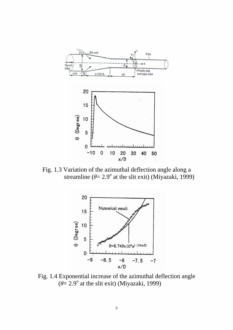
Miyazaki et al. (1999) investigated the spiral flow by introducing a very small azimuthal motion at the exit of the annular slit. He obtained that in his simulation study the azimuthal deflection angle of a streamline quickly enlarges through the annular jet ejected from the slit exit, and the enlargement processes can be described by exponential curves and the spiral phenomenon can be easily simulated as a quick increase in the azimuthal deflection angle of streamlines, which is sufficiently large in value due to the formation of a spiral structure of a streamline and proposed that the rapid enlargement of the azimuthal deflection angle may be attributed to circulation conservation in the contraction process of the vortex tube in the annular jet (Fig. 1.3 and Fig. 1.4).

Matsuo et al. (2003) investigated about the effect of the geometry of annular slit on the flow characteristics of spiral jet experimentally by using the two-component LDV system. From the experimental results, he reported that the flow characteristics of spiral jet could be divided into three types; type A: tangential velocity component is small and has a asymmetric distribution, type B: tangential velocity component is intermediate and has a nearly symmetric distribution, and

4

type C: tangential velocity component is large and has a nearly symmetric distribution, following the tangential velocity distributions in the present experimental conditions (Fig. 1.5).

In the most recent, Cho et al. investigated the internal flow characteristics of spiral flow nozzle using computational technique and presented that the tangential component in the spiral flow nozzle changes as the geometry of nozzle and conditions etc.

In spite of these efforts, the understanding for the self-generating mechanism of the tangential velocity component in nozzle is not still enough to be satisfactory. The understandings for the control of initial tangential component self-generated in the nozzle and detailed internal flow characteristics to apply in the field of a variety of industrial are inevitable. It is thought that the rapid advancement in computer industry and rapid development in the technology of numerical analysis will give the solutions for these problems not to be solved.

1.2 Objectives of Research

In the meaning of having tangential momentum in the flow characteristics, the spiral flow which is self-generated in the Coanda nozzle can be included in the category of swirling flow and be thought that it is not a new technology and phenomenon at all in such thing. However, since the tangential momentum in the spiral flow is self-generated by unique nozzle configuration, it can be treated as new one.

In present, the spiral flow generated by the Coanda nozzle, the unit which is composed of air chamber, annular slit, Coanda surface and conical cylinder has been applying in a various field such as soil and granule transportation, dispersion and encapsulation of submicron powders, cutting of soft materials, optical fiber passing, concentration of a plasma energy flow and so on.

However, as mentioned before section, the study about its generating mechanism and control method is not enough to make us understand. Therefore, the understanding on the self-generated mechanism of tangential component in Coanda nozzle is still the worth of challenge and its control is very important for more applications than now.

In this thesis, the primary objectives are newly to clarify the self-generated

5

mechanism of the spiral flow in Coanda nozzle and to get better understanding on its detailed flow characteristics. Finally, the effect of the change of nozzle configuration and initial conditions is tried to understand.

1.3 Overview of Thesis

The background, motivation and research progress of swirling and spiral flow have been briefly explained in Chapter 1. The principal objectives of the present study are also described in this chapter. Research results and the theory of the generated mechanism of the spiral flow by other researchers are followed in Chapter 2. The fundamental flow characteristics and application field used in present are explained in this chapter.

Chapter 3 gives the description of the experimental apparatus used in the present work. This includes a description of high pressure air supply system, LDV system and nozzle configuration.

Chapter 4 explains the basic information by the numerical analysis and turbulence model used in this thesis.

From Chapter 5 to Chapter 6, at first, the comparison of the results from the experiment and computation is carried out and the self-generated mechanism of the spiral flow in Coanda nozzle based on these results is proposed. The flow features with the change of pressure ratio and nozzle geometry are described. Finally, Chapter 7 summarizes the important findings obtained from Chapter 5 through Chapter 6.

6

(a) Typical jet flow by conventional nozzle

(b) Spiral jet flow by Coanda nozzle

Fig. 1.1 Visualization of jet flow (Horii, 1991)

(Re = 2.1×104)

7

(a) Axial turbulent intensity

(b) Tangential velocity component (u=10m/s)

Fig. 1.2 Characteristics of turbulent swirling flow

in a straight pipe (Nishizaka, 1994)

8

Fig. 1.3 Variation of the azimuthal deflection angle along a streamline (θ = 2.9o at the slit exit) (Miyazaki, 1999)

Fig. 1.4 Exponential increase of the azimuthal deflection angle (θ = 2.9o at the slit exit) (Miyazaki, 1999)

9

(a) Type A (RL5, R5) (b) Type B (RL4, R3)

(c) Type C (RL1, R1)

Fig. 1.5 Tangential velocity distributions (Matsuo et al., 2003) (pos=110.9 kpa, z / DH =0.5)

; pos : stagnation pressure upstream of annular slit, z : axial direction

10

CHAPTER 2

PREVIOUS THEORY OF SPIRAL FLOW

In this chapter, the self-generating mechanism of the spiral flow in the spiral nozzle suggested by previous researchers, the general features of spiral flow and its structure and the applications which are being used in present are described briefly.

2.1 The Structure of Spiral Flow Nozzle

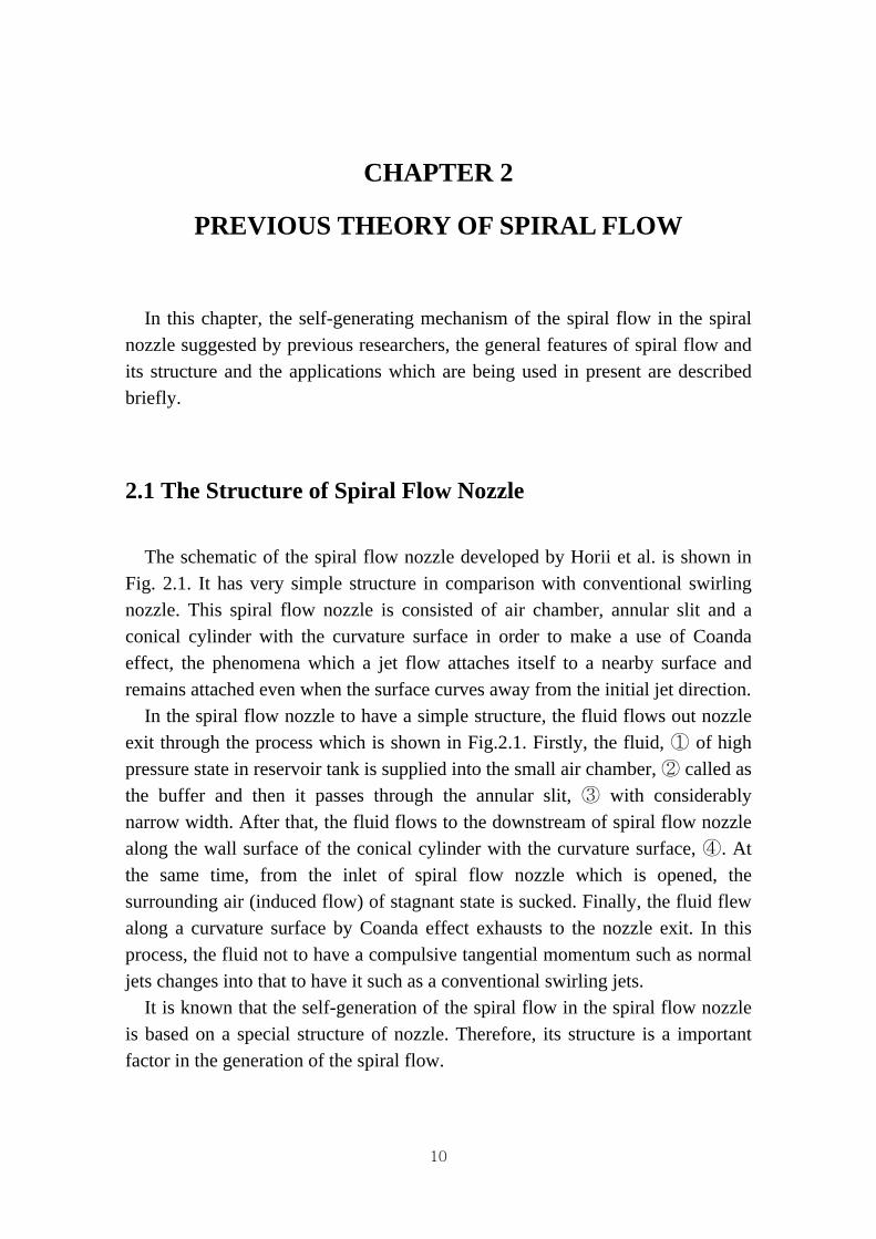
The schematic of the spiral flow nozzle developed by Horii et al. is shown in Fig. 2.1. It has very simple structure in comparison with conventional swirling nozzle. This spiral flow nozzle is consisted of air chamber, annular slit and a conical cylinder with the curvature surface in order to make a use of Coanda effect, the phenomena which a jet flow attaches itself to a nearby surface and remains attached even when the surface curves away from the initial jet direction.

In the spiral flow nozzle to have a simple structure, the fluid flows out nozzle exit through the process which is shown in Fig.2.1. Firstly, the fluid, ① of high pressure state in reservoir tank is supplied into the small air chamber, ② called as the buffer and then it passes through the annular slit, ③ with considerably narrow width. After that, the fluid flows to the downstream of spiral flow nozzle along the wall surface of the conical cylinder with the curvature surface, ④. At the same time, from the inlet of spiral flow nozzle which is opened, the surrounding air (induced flow) of stagnant state is sucked. Finally, the fluid flew along a curvature surface by Coanda effect exhausts to the nozzle exit. In this process, the fluid not to have a compulsive tangential momentum such as normal jets changes into that to have it such as a conventional swirling jets.

It is known that the self-generation of the spiral flow in the spiral flow nozzle is based on a special structure of nozzle. Therefore, its structure is a important factor in the generation of the spiral flow.

11

2.2 Self-generating Mechanism of Spiral Flow

The self-generating mechanism of spiral flow in this spiral flow nozzle by the flow process mentioned in section 2.1 is going to be introduced in this section. Fig.2.2 describes the generation of initial swirl velocity. First, the cross-sectional surface, s normal to z axis is taken. It is assumed that the annular slit of spiral flow nozzle is manufactured uniformly. Then, it can be thought that the initial velocity component of the compressed air passing through annular slit is only that in radial direction. In this case, the angular momentum is not occurred in annular slit by the axi-symmetric structure of nozzle. If the fluid from annular slit, however, has a strong turbulence by a transient flow state, the situation is to be changed. In the other words, instant radial velocity, Ävr can be divided into mean velocity, vr and variable velocity, vr’. It means that the angular momentum through annular slit is existed. If the Reynolds number is increased, its potential for the generation of angular momentum will be higher. However, although Ävθ by the situation as explained generates, its time-averaged value is to be zero. However, its state changes if both Ävθ and Ävz have considerably high value together. If its situation assumes that is occurred in time, to, the point, P on the surface, s moves to a point on the surface, s’ in time, to + Δt by the composition of velocity components Ävr, Ävθ, and Ävz as shown in Fig.2.3. It is sustained to nozzle exit and its value amplifies gradually as goes to nozzle exit since total angular momentum is conserved by the configuration of the type of conical cylinder.

However, since this phenomenon is generated probably by the flow state, it is very difficult to estimate its rotational direction. As a result, the essential conditions for self-generation of spiral flow in the spiral flow nozzle are high axial velocity by Coanda effect, strong turbulent intensity in radial velocity component and nozzle structure. From these compositions, the spiral flow to have long rotational pitch and high axial velocity and so on is generated in the spiral flow nozzle.

12

2.3 The General Features of Spiral Flow

In comparison of a conventional swirling jet and normal jet, the self-generated spiral flow in the spiral flow nozzle has some different flow characteristics. In general, normal jets have high flow variation and unstable features, while spiral flow has low variation and good stability with the time. Moreover, in comparison of a conventional swirling flow to have a broad forced vortex region and vortex breakdown in high swirl ratio, it has a comparable flow features such as smaller vortex core, lower swirl decay, sustaining ability over a long distance in the pipe. Axial velocity distribution

Fig.2.4 shows the distributions of axial velocity in the nozzle. In figure, the axial velocity in the position, B at near annular slit has maximum value near internal wall surface since the flow flews along the curvature surface by Coanda effect and its value in the center is low relatively by the decrease of static pressure. Thus, its distributions in radial direction becomes the type of W. Its maximum value in C moves the center of nozzle in internal wall surface and it becomes the type of M. In the position of D and E, its maximum is found around the center of nozzle. As a result, the variation of axial velocity distribution can be divided into three patterns.

The flow features of the spiral jet to a general normal jet by the results obtained in several appointed positions from nozzle exit are showing in Fig.2.5 and Fig.2.6. In the case of the spiral flow, the axial velocity is very high around the axis in comparison of normal jet. Thus, it shows steeper axial velocity distributions. In addition, the length of potential core in the spiral flow is longer than that of normal jet. The turbulent intensity of axial velocity and the width of jet in Fig.2.7 are relatively smaller and narrower than that of normal jet. From these results, it is confirmed that the spiral flow is stable relatively in comparison of normal jet. Radial velocity distribution

The features of radial velocity in the spiral flow are showing in Fig.2.7 and Fig.2.8. In the radial distributions of radial velocity, it follows such a general trend as the features obtaining in the nozzle flow of the type of conical cylinder. However, the radial turbulence intensity is getting higher gradually near internal

13

wall surface and lower gradually around the axis. Tangential velocity distribution

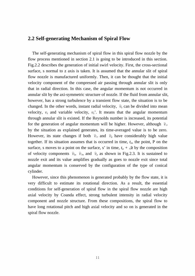
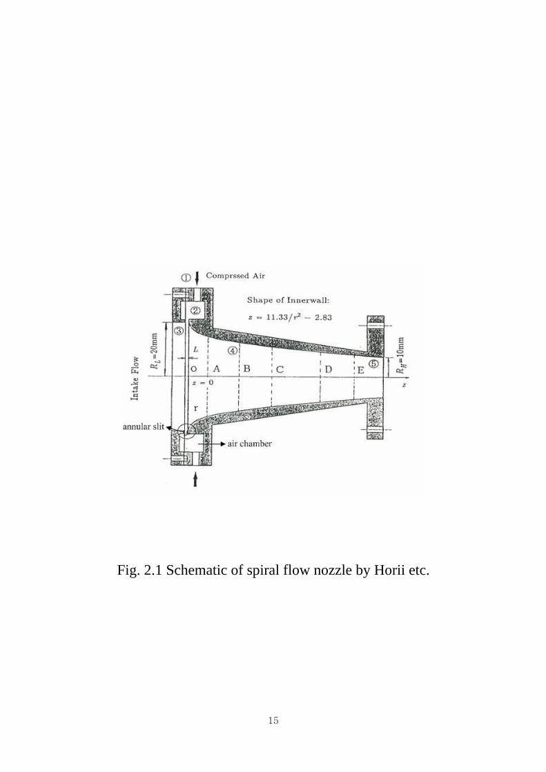
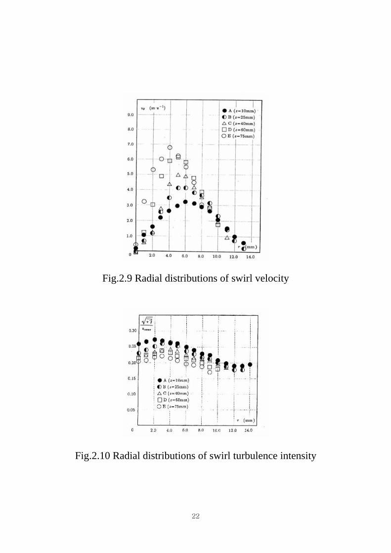
Fig.2.9 shows radial distributions of swirl velocity. Despite of not giving a tangential force, swirl velocity is detected at each position in the nozzle and its value grows as goes to nozzle exit. Finally, in the position, E swirl velocity has maximum value. These features can be explained by the momentum conservation in the swirl tube. Furthermore, the swirl intensity by the swirl velocity in the nozzle also increases gradually as goes to nozzle exit and swirl turbulence intensity as shown in Fig.2.10 decreases gradually.

2.4 Applications of Spiral Flow

As mentioned before section, the spiral flow has the flow features such as the high convergence in axial velocity, wide free vortex region and low swirl ratio unlike conventional swirling flow and normal jet. Because of these reasons, it is applying in many industrial fields. In this section, the applications will be introduced.

2.4.1 Inspection system for pharmaceutical conveying pipeline [11], [73]

In pharmaceutical industry, it is very important for the pipeline used in order to transport materials to keep clean, since it is related to the health of users who use it. Then, this problem can give a vital loss to the company to make it. For these reasons, developing a special device to inspect the pipeline may be a hot issue in the company related with these problems. Fig. 2.11 shows the schematic of the inspection system for pipeline using the feature of spiral flow. This system is composed of parachute connected with the tip, CCD camera to collect the images, optical cable to link these and spiral flow nozzle.

2.4.2 Soil transporter in construction side [66]

Dredged mud transportation for seaside airport construction requires minimum environmental impact and high efficiency. However, one conventional

14

transportation method was not satisfied with these demands in an environmental impact and high cost. Recently, the use of a certain kind of spiral flow nozzle provides a good new possibility for replacing the vacuum pump in conventional pneumatic transportation systems.

2.4.3 Pipe cleaning technology [74]

Nuclear power plants will be discontinued and scrapped sometime after its long-time operation, but it is very imperious to clean the waste coming out of the plants, reduce its radioactive contents and protect the scrapping workers against the radioactivity. Therefore, the development of an efficient cleaning method has been called for. Fig. 2.12 shows a diagram of this system. It can be achieved using the spiral flow nozzle with an abrasive material. Using this spiral flow, it is possible to clean the inside of a pipe by its flow features.

In addition to these applications, in present, the spiral flow is applying in many various industrial fields such as the coating technology by water jet, the focusing control for dispersion of submicron powder, focusing and stability control of plasma jet, water jet cleaning, orientation control of whiskers for producing new composites, transportation of optical fiber through 2000m-long tubes, and stability control of burners' flames.

15

Fig. 2.1 Schematic of spiral flow nozzle by Horii etc.

16

Fig. 2.2 Generation of initial swirl velocity

17

Fig. 2.3 The generating mechanism of spiral flow

18

(a) Sketch of the variations of axial velocity in the nozzle

(b) Radial distributions of axial velocity

Fig. 2.4 Distributions of axial velocity in the nozzle

19

(a) Normal jet

(b) Spiral jet

Fig. 2.5 Axial velocity distributions of jet

20

(a) Normal jet

(b) Spiral jet

Fig. 2.6 Turbulent intensities of axial velocity

21

Fig.2.7 Radial distributions of radial velocity

Fig.2.8 Radial distributions radial turbulence intensity

22

Fig.2.9 Radial distributions of swirl velocity

Fig.2.10 Radial distributions of swirl turbulence intensity

23

Fig. 2.11 Schematic of inspection system for pipe

Example of cleaning the thin heat transfer pipe in heat exchanger

Fig. 2.12 Cleaning system using the spiral flow

24

CHAPTER 3

EXPERIMENTAL APPARATUS

AND PROCEDURE

In this chapter, the experimental apparatus and procedure used in this study is described. The results obtained from the experiment will be used in order to check the validation of numerical analysis.

3.1 Experimental Apparatus

The schematic of experimental apparatus used in this study is shown in Fig.3.1.

The experimental apparatus is approximately consisted of two parts; part 1 and part 2.

At first, part 1 is the apparatus to supply the pressurized air in the test section. These are composed of four units; compressor to pressurize air, air cleaner to make a clean a polluted air, air drier to remove the moisture with air and reservoir(tank) of disposed air. Part 2 is the test section to measure velocity components of flow discharged from spiral nozzle used in the experiment. This part 2 is composed of circular duct with tube connector to supply the pressurized air in the four ports of spiral nozzle, particle generator, pressure gauge to measure pressure in the buffer section of Coanda nozzle and LDV (Laser Doppler Velocimeter) to measure velocity components of flow discharged from the spiral nozzle.

Each unit in part 1 and part 2 is connected to circular duct with metal pipe and the pressure in the buffer section of Coanda nozzle unit is controlled by the use of the valve in front of circular duct. Four rubber tubes attached with circular duct are used to supply the buffer section with the pressurized air generated from part 1. The pressure in the buffer region becomes reference pressure, po to determine the pressure ratio of the pressure in the buffer to ambient pressure, pa.

For the measurement of flow velocity by the use of LDV system, water-

25

particle with roughly diameter of 4μm generated from ultrasonic humidifier is used as seed. Therefore, the ultrasonic humidifier is located in nozzle inlet.

The Coanda nozzle unit used in this experiment is shown in Fig.3.2. The width of annular slit used in this test is 0.6mm. The radius of nozzle exit, RH and nozzle inlet, RL is 10mm and 23.28mm, respectively. And the radius of curvature surface connected with the tip of annular slit, R and the length of nozzle, H is 5mm and 85mm respectively.

3.2 Experimental Procedure

3.2.1 Velocity measurement

The measurement of the high velocity profile inside and outside the nozzle or ejector is very difficult since it disturb the flow discharged from themselves. If a pitot tube or hot wire is used to measure it, they will disturb the flow, resulting in inaccurate measurements. However, if the LDV system is used, it will not disturb the flow that is needed. Therefore, in this study, the LDV system (Aerometrics Ltd. 2D-LDV/RSA) for the measurement of flow velocity is used. This LDV system consist an argon-ion laser, a multicolor beam separator, a two-component fiber-optic probe system, signal processor, a 3-D traverse table driven by interface, and a personal computer with the flow information software. The measurement of flow velocity in the nozzle exit shows in Fig.3.3. The measurement of flow velocity is carried at the specific distance, z / DH = 0.5, 2.0 from the exit of Coanda nozzle. Also, the measurement of flow velocity at each measuring position is done by the movement of LDV probe every 2mm by the use of the traverse system along the cross-sectional direction from the central axis. At this time, sampling number of each measuring point is approximately 10,000 to reduce the uncertainty of data. Finally, axial velocity component, vz and tangential velocity component, vθ as shown in Fig.3.4 are obtained.

As mentioned in section 3.1, the water-particle generated by ultrasonic humidifier in the vicinity of nozzle exit is used as seed of LDV system. This water-particle size with the diameter of mμ4 is small enough to minimize errors in velocity measurements resulting from acceleration effects on the seed particles. The Doppler-frequency of each channel is transformed into two velocity

26

components through two real-time signal analyzers (RSA). By this transformation, two velocity components (axial and tangential velocity) can be obtained. 3.2.2 Pressure measurement

In the study, the existence of the pressurized air supplied into the buffer of spiral nozzle unit through four rubber tubes is very important. If the pressure of the pressurized air supplied is not equal to each other, it has no meaning because the unbalance of the pressure of air supplied through them can result in the tangential velocity in the buffer. As a consequence, the measurement of the pressure in the buffer is a key point in this test.

In order to monitoring the pressure supplied in the buffer, it is measured in four points such as Fig. 3.5 with digital pressure gauge which is connected with PC. Thus, we can check the variation of pressure in real time through PC. As a result, the difference of the pressure in four measuring points for pressure in the buffer is not found after the flow is fully developed. It means that the air pressure supplied into four tubes is same and the test apparatus has the reliability.

The state in the buffer after the flow is fully developed can be assumed as stagnation one. It means that the pressure measured in the buffer with digital pressure gauge is almost equal to stagnation pressure (total pressure). This result is applied to the computational test as initial or reference condition.

27

Fig. 3.1 Schematic of experimental apparatus

28

Fig. 3.2 Schematic of Coanda nozzle

29

Fig. 3.3 Measurements of spiral flow

30

(a) Measurements of the axial velocity component

(From the top of experimental apparatus)

(b) Measurements of the tangential velocity component

(From downstream side)

Fig. 3.4 Measurements of the velocity component

31

Fig. 3.5 Measurements of pressure

32

CHAPTER 4

NUMERICAL ANALYSIS The flow under considering in this study is unsteady, three dimensional compressible flow. In order to analyze it, the computational code (UPACS, Unified Platform for Aerospace Computational Simulation) which is freely distributing for research is used and it was developed from JAXA (Japan Aerospace Exploration Agency). It is based on the Navier-Stokes equations using FVM (Finite Volume Method) and parallel computing system.

In this chapter, a brief introduction for this code, the governing equation and numerical method used will introduce briefly.

4.1 Brief introduction of UPACS In recent, the advancement of computing technology and computer industrial has played an important role in the flow analysis. However, it is the fact that the CFD for the flow analysis is not easy for researchers to understand and universal for all flows. And the computational code based on the parallel computing in order to reduce the analysis time is not so much yet. Since these problems, the easier and stronger computational tools based on parallel computing have been demanded. From these demands, UPACS (Unified Platform for Aerospace Computational Simulation) is made from JAXA in Japan. This is freely distributed for research under some regulations in Japan. Several features of UPACS code is introduced as follows;

- Separation of parallel computation and Solver - The adoption of Multi-block grid(Structure grid) - Hierarchical Structure - Management of parameter by module etc.

33

4.2 Basic Equations In this section, the basic equations used in this code will be introduced. At first, the physical model assumed is going to be described. The governing equation based on this physical model and non-dimensionalization for the governing equations will also be introduced, subsequently. Finally, the parameters related with non-dimensionalization will be explained. 4.2.1 Physical model - Physical model under considering in UPACS

• Specific heat is constant • Compressible flow • Viscosity(Sutherland Formulation) • Three dimensional flow • RANS(Turbulence Model) • No external force including gravity etc.

4.2.2 Governing equations The compressible Navier-Stokes equations in Cartesian coordinates without body force or external heat addition were used describe the flow fields. The equations were written as

)3,2,1,(0 ==∂∂

+∂∂

+∂∂ ji

xFv

xF

tQ

j

j

j

j (4.1)

Eq.(4.1) indicates the governing equation by tensor notation. Where Q is

solution vector, Fj is inviscid flux vector, and Fvj is viscous flux vector, respectively. Q, Fj and Fvj can be expressed as below by tensor notation;

⎟⎟⎟

⎠

⎞

⎜⎜⎜

⎝

⎛

=

E

uQ jρρ

(4.2)

34

⎟⎟⎟⎟

⎠

⎞

⎜⎜⎜⎜

⎝

⎛

+=

Hu

puu

u

F

j

ijij

j

j

ρ

δρ

ρ

(4.3)

⎟⎟⎟⎟⎟⎟⎟

⎠

⎞

⎜⎜⎜⎜⎜⎜⎜

⎝

⎛

∂∂

+

=

jiij

ijj

xTku

Fv

τ

τ0

(4.4)

Internal energy is

2

21, jueEe ρρε +== (4.5)

TCv=ε (4.6)

2

21

1 juppEH +−

=+

=ργ

γρ

(4.7)

where H is enthalpy, Stress tensor is

)3,2,1,(32

=⎟⎟⎠

⎞⎜⎜⎝

⎛

∂∂

−∂∂

+∂∂

−= jixu

xu

xu

ijk

k

i

j

j

iij δμτ (4.8)

tl μμμ += μl and μt were the laminar and turbulent viscosity. Thermal conductivity, k can be expressed as follows,

)1( −

=γμγ

rPRk (4.9)

Where Pr is the Prandtl number and is defined as following;

59

4−

==γγμ

kC

P pr (4.10)

35

The fluid is a perfect gas. Hence, the equation of state takes following form;

RTp ρ= (4.11)

The equation to get the sound of speed is calculated by (4.12)

RTpc γρ

γ ==2 (4.12)

The thermal conduction term in (4.4) can be expressed using (4.9) and (4.12) as following;

jrj xc

PxTk

∂∂

−=

∂∂ 2

)1(γμ (4.13)

4.2.3 Non-dimensionalization

There is the explanation for non-dimensionalization of each variable. In this study, a mean flow for external flow and stagnation point for internal flow like turbo machinery is used as reference state for non-dimensionalization of each variable. The value in reference state is shown with subscript, *. 4.2.3.1 Basic non-dimensional variables

Where *ρ , *u and *L are density, velocity, and characteristic length in reference state, respectively. The variables which are non-dimensionalized as below are obtained by each variable in reference state.

Density ( ρ )

)(,ˆ *ρρρρρ == oo (4.14)

Velocity (with the speed of sound, *c in reference state)

)(,ˆ *ccucu oo == (4.15)

Characteristics Length (L)

)(,ˆ *LLxLx oo == (4.16)

36

The value of reference state is equal to one which is non-dimensional for these variables but the values which are non-dimensional below are different from the values in reference state.

*ppo ≠ (4.17)

*TTo ≠ (4.18)

*μμ ≠o (4.19)

The equation for speed of sound in reference state is equal to

**

*2* RTpc γ

ργ == (4.20)

4.2.3.2 Non-dimensionalization of each variable

Non-dimensionalization of each variable is as follows by the use of the value of reference non-dimensional.

Time(t) )(ˆo

oo

o

o

cLtt

cLt == (4.21)

Pressure(p) )(ˆˆ 22oooooo cppcppp ρρ === (4.22)

In here, non-dimensional value of pressure, op is obtained from (4.20)

)( **2**

2 ppccp ooo ≠=== γρρ (4.23)

po in (4.23) is different from the pressure in reference state, *p . The equation to get speed of sound is as following,

ργ pc =2 (4.24)

ρρργ

ρργ

ˆˆ

ˆˆˆ

222

o

oo

o

oo

pcppcc == (4.25)

37

ργ

ˆˆˆ2 pc = (4.26)

As above, the form of equation to get speed of sound is to be same in both dimension and non-dimension.

Viscosity Coefficient (μ )

)(ˆˆ oooooooo LcLc ρμμρμμμ === (4.27)

Temperature (T )

)(,ˆˆ22

RcTT

RcTTT o

oo

o === (4.28)

In here, non-dimensional temperature, oT is obtained by (4.20)

)( **

2*

2

TTRc

RcT o

o ≠=== γ (4.29)

This is different from the temperature, *T in reference state. Thus, the equation to get speed of sound is as follows;

RTc γ=2 (4.30)

TRcR

TRTcc

o

oo

ˆ

ˆˆ2

22

γ

γ

=

= (4.31)

Tc ˆˆ2 γ= (4.32)

And the equation of state of ideal gas

RTp ρ= (4.33) is derived as following;

TRcRpc o

oooˆˆˆ

22 ρρρ = (4.34)

38

Tp ˆˆˆ ρ= (4.35)

If the relation expression between internal energy and pressure (4.36) is non-dimensional, the relation expression can be expressed as (4.37)

TCp vργρεγ )1()1( −=−= (4.36)

TRTRp

TRcCpc o

vooo

ˆˆˆ

1ˆ)1(ˆ

ˆˆ)1(ˆ2

2

ργ

ργ

ρργρ

=−

−=

−= (4.37)

where is RCC vp =− ,

vCR

=−1γ , and 1−

=γ

RCv .

4.2.3.3 Viscosity coefficient

In this study, the Sutherland’s Law is used to obtain the coefficient of viscosity. It can be expressed using the coefficient of viscosity, μs in the temperature, Ts as follows;

⎟⎠⎞

⎜⎝⎛

++

⎟⎟⎠

⎞⎜⎜⎝

⎛=

STST

TT s

ss

5.1

μμ (4.38)

If the temperature, Ts in (4.38) is guessed as the temperature, *T in reference state, μ in the Sutherland’s Law can be expressed as below;

⎟⎟⎟⎟

⎠

⎞

⎜⎜⎜⎜

⎝

⎛

+Θ

+Θ=

⎟⎟⎟⎟

⎠

⎞

⎜⎜⎜⎜

⎝

⎛

+

+

⎟⎟⎠

⎞⎜⎜⎝

⎛=

*

*5.1*

**

*

5.1

**

11

TS

TS

TS

TT

TS

TT μμμ (4.39)

where Θ is equal to (4.40), and by using (4.29) or (4.32) it is derived respectively,

39

** TT

TT

γγ

==Θ (4.40)

)( *TTTT

oo

γγ==Θ (4.41)

2c=Θ (4.42)

Thus, following expression is derived by non-dimensional with (4.27)

⎟⎟⎟⎟

⎠

⎞

⎜⎜⎜⎜

⎝

⎛

+Θ

+Θ=

*

*5.1*

1ˆ

TS

TS

Lc ooo μμρ (4.43)

⎟⎟⎟⎟

⎠

⎞

⎜⎜⎜⎜

⎝

⎛

+Θ

+Θ′

=

⎟⎟⎟⎟

⎠

⎞

⎜⎜⎜⎜

⎝

⎛

+Θ

+Θ=

*

*5.1

*

*5.1*

11

1ˆ

TS

TS

RTS

TS

Lc eoooρμμ (4.44)

In here, where eR′ is Reynolds number in the reference state.

*

***

* μρ

μρ LcLcR ooo

e ==′ (4.45)

4.2.4 Mach number and Reynolds number

In this computational code, the Mach number in reference state in order to get a relation between the reference state and stagnation point which is used in the calculation of boundary condition is fixed as a constant value. Then, in order to be non-dimensionalized the viscosity coefficient, the Reynolds number (flow_ref_Reynolds) and temperature (flow_ref_T) in reference state is given respectively.

In the definition of Reynolds number used in a general experiment, uniform flow is used to calculate them. However, in this code, since the method to get it is different, the caution is required. For example, if the velocity of uniform flow, V* is given to obtain Reynolds number Re, the Reynolds number which is used in this study is as follows,

40

**

*

*

*

*

***

*

*** 1M

RVcR

VcLVLcR eee ×=×===′

μρ

μρ (4.46)

Where *M is Mach number calculated using the sound of speed, *c in reference state. The grid for computation is assumed to be non-dimensional with characteristics length, *L and it is different value from characteristics length, Lexp used in general experiment,

exp

*

*

exp

*

*

*

*

exp**

*

***

1LL

MR

LL

VcLVLcR

e

e

×=

==′μ

ρμ

ρ

(4.47)

4.2.5 Non-dimensionalization of governing equations 4.2.5.1 Non-dimensionalization of continuity equation The continuity equation in (4.1) is to be non-dimensional by (4.21)

0ˆ

ˆˆˆˆ

=∂

∂+

∂∂

jo

joo

o

o

xLuc

ttρρρρ (4.48)

0ˆˆˆ

ˆˆ

=∂

∂+

∂∂

j

j

o

oo

o

oo

xu

Lc

tLc ρρρρ (4.49)

0ˆˆˆ

ˆˆ

=∂

∂+

∂∂

j

j

xu

tρρ (4.50)

4.2.5.2 Non-dimensionalization of momentum equation From (4.4), stress tensor, τij is

41

ijoo

ijk

k

i

j

j

ioo

ijk

k

i

j

j

i

o

oooo

ijko

ko

io

jo

jo

iooij

c

xu

xu

xuc

xu

xu

xu

LcLc

xLuc

xLuc

xLuc

τρ

δμρ

δμρ

δμμτ

ˆ

ˆˆ

32

ˆˆ

ˆˆˆ

ˆˆ

32

ˆˆ

ˆˆˆ

ˆˆ

32

ˆˆ

ˆˆˆ

2

2

=

⎟⎟⎠

⎞⎜⎜⎝

⎛

∂∂

−∂

∂+

∂∂

−=

⎟⎟⎠

⎞⎜⎜⎝

⎛

∂∂

−∂∂

+∂∂

−=

⎟⎟⎠

⎞⎜⎜⎝

⎛

∂∂

−∂

∂+

∂∂

−=

(4.51)

By using it, following equations are given;

0ˆˆ

ˆ)ˆˆˆˆˆ(ˆˆ 22

=∂∂

+∂

+∂+

∂∂

jo

ijoo

jo

ijojioo

o

joo

xLc

xLppuuc

ttuc τρδρρρρ

(4.52)

0ˆˆ

)ˆˆˆˆˆ(ˆˆ

ˆˆ 222

=∂∂

++∂∂

+∂∂

j

ij

o

oijji

jo

oj

o

o

xLcpuu

xLc

tu

Lc τρδρρρρ (4.53)

0ˆˆ

)ˆˆˆˆˆ(ˆˆ

ˆˆ=

∂

∂++

∂∂

+∂

∂

j

ijijji

j

j

xpuu

xtu τ

δρρ

(4.54)

In general, Reynolds number in viscous term is included in non-dimensional Sutherland’s expression to obtain viscosity. 4.2.5.3 Non-dimensionalization of energy equation The equation of energy conservation, (4.5) can be expressed as following by non-dimensionalization,

EcuecucecE oojoojooooˆˆˆ

21ˆˆˆ

21ˆ 222222 ρρρρρρ =⎟

⎠⎞

⎜⎝⎛ +=+= (4.55)

and the equation for enthalpy from (4.7) is to be (4.56)

HcpEcpcEcH ooo

oooo ˆˆ

ˆˆˆ

ˆˆ22

22

=+

=+

=ρρρ

ρρ (4.56)

42

Thus, totally energy equation by non-dimensionalization can be expressed such as (4.47), (4.58) and (4.59),

0ˆ

)ˆˆ

)1(ˆˆˆ(

ˆ

ˆˆˆˆ

223

32

=∂

∂∂

−+∂

+∂

∂+

∂∂

jo

jo

o

r

oooiijoo

jo

joo

o

oo

xLxLcc

PLcuc

xLHuc

ttc γ

μρτρρρρ (4.57)

0ˆˆ

)1(ˆˆˆ

ˆˆ

ˆˆˆˆˆ 2333

=⎟⎟⎠

⎞⎜⎜⎝

⎛

∂∂

−+

∂∂

+∂

∂+

∂∂

jriij

jo

oo

j

j

o

oo

o

oo

xc

Pu

xLc

xHu

Lc

tE

Lc

γμτρρρρ (4.58)

0ˆˆ

)1(ˆˆˆ

ˆˆ

ˆˆˆˆˆ 2

=⎟⎟⎠

⎞⎜⎜⎝

⎛

∂∂

−+

∂∂

+∂

∂+

∂∂

jriij

jj

j

xc

Pu

xxHu

tE

γμτ

ρ (4.59)

4.3 Numerical Method 4.3.1 Discretization

The numerical solution of the differential equations that describe fluid flows usually involves the introduction of a series of distinct nodal points over the solution domain and then the solution of the numerical form of the governing equations to give the values of the flow variables at these nodal points rather than for their values continuously over the whole flow field. To do this, some form of numerical approximation for the derivatives in the governing equations is introduced. These numerical approximations for the derivatives, which are expressed in terms of the values of the values of the variables at the nodal points, can be obtained in a number of different ways. In this numerical method, the finite volume method is used.

As mention above, if the cubic cell which is made by grid generation, regards as control volume, integral equation (4.1) for cubic cell can be discretized as (4.60). At this time, the matrix such as the volume and area of cell, and normal vector can directly get from the grid under consideration. In here, as simple and easy example, the discretization of governing equation for Euler’s explicit method will be explained. The governing equation, (4.1) by this discretization

43

can briefly be expressed as following,

))(

)()((

21

21

21

21

21

21

21

21

21

21

21

21

1

−−++

−−++−−++

+

−

−−−ΔΔ

+=

knkk

nk

jnjj

nji

nii

ni

nn

dAdA

dAdAdAdAVt

FF

FFFFQQ (4.60)

where Q and F is the conservation mass term and inviscid flux term, respectively. 4.3.2 Calculation of matrix

In this section, the calculation of Matrix is expressed. The cubic cell in Fig.4.1 is considered. At first, the matrix is calculated for the cell xi, i = 1, 8 in Fig.4.1 as follows;

Fig.4.1 Cubic cell

Cell center :

∑=

=8

1,, ,

81)(

iikjic xx (4.61)

Surface center :

)(41)(

)(41)(

)(41)(

766521

874321

763221

xxxxx

xxxxx

xxxxx

kFC

jFC

iFC

+++=

+++=

+++=

+

+

+

(4.62)

44

The distance of cell center and surface center :

ckFCk

cjFCj

ciFCi

xx

xx

xx

−=Δ

−=Δ

−=Δ

+

+

+

21

21

21

)(

)(

)(

(4.63)

Volume : volume is calculated to divide into six surfaces

)))(())(())(())((

))(())()(((61)(

12161615

15181814

1413131217,,

xxxxxxxxxxxxxxxx

xxxxxxxxxxdV kji

−−+−−+−−+−−+

−−+−−−=

(4.64)

Normal Vector :

))((21)(

))((21)(

))((21)(

685721

473821

362721

xxxxdA

xxxxdA

xxxxdA

k

j

i

−−=

−−=

−−=

+

+

+

n

n

n

(4.65)

Differential of ζηξ and, :

ii

iz

iii

iy

iii

ix

i

ii

iz

iii

iy

iii

ix

i

ii

iz

iii

iy

iii

ix

i

dVdV

dAn

zdVdV

dAn

ydVdV

dAn

x

dVdV

dAn

zdVdV

dAn

ydVdV

dAn

x

dVdV

dAn

zdVdV

dAn

ydVdV

dAn

x

+=

∂∂

+=

∂∂

+=

∂∂

+=

∂∂

+=

∂∂

+=

∂∂

+=

∂∂

+=

∂∂

+=

∂∂

+

+

++

+

++

+

+

+

+

++

+

++

+

+

+

+

++

+

++

+

+

1

21

21

1

21

21

1

21

21

1

21

21

1

21

21

1

21

21

1

21

21

1

21

21

1

21

21

)(2)(,

)(2)(,

)(2)(

)(2)(,

)(2)(,

)(2)(

)(2)(,

)(2)(,

)(2)(

ζζζ

ηηη

ξξξ

(4.66)

45

4.3.3 Convective term Roe (FDS scheme) (P.L.Roe, 1981) and AUSMDV (FVS scheme) (Y.Wada

and M.S. Liou, 1994, 1997) scheme for convective term make use of in this code. In this study, Roe scheme was employed. For example, in Roe scheme, velocity is calculated by (4.67).

)(~~~21))()((

21),( LRL

CR

CLR

C QQLΛRQFQFQQF −−+= (4.67)

RQ and LQ are physical variables in both sides of cell. These are given in the distribution of physical variables of internal cell and the limiter for the stability of calculation (MUSCL method) is used. But the flow under considering in this study is not included a strong variation of physical variable like shock wave. Thus, it will be taken into account for the use of the limiter.

Fig.4.2 Cell used in extrapolation

Fig.4.2 shows the cell that is used in extrapolation. L~ , R

~ and Λ~ mean

eigenvector and eigenvalue, respectively. In this study, these values are as below,

)~,~,~,~,~(~ cUUUUcUdiag −+=Λ

⎥⎥⎥⎥⎥⎥⎥⎥⎥⎥⎥

⎦

⎤

⎢⎢⎢⎢⎢⎢⎢⎢⎢⎢⎢

⎣

⎡

−+⋅

+⋅

+⋅

+

−−++

−+−+

−−++

=

UcHV

cuunV

cuun

Vc

uunUcH

ncw

cwnn

cwn

ncwnn

cw

ncvn

cvn

cvn

ncvnn

cv

ncun

cunn

cun

cunn

cu

ccn

cn

cn

c

zz

yy

xx

zz

xy

yx

z

yxzy

zx

y

xyz

zyx

x

zyx

~~

2

~~

2

~~

2

~~~~

~~~~~

~~~~~

~~~~~

11

~R

46

⎥⎥⎥⎥⎥⎥⎥⎥⎥⎥⎥

⎦

⎤

⎢⎢⎢⎢⎢⎢⎢⎢⎢⎢⎢

⎣

⎡

−−−−−−−−−−−

⋅−

−−−+−−−−+

⋅−−

−−−−−+−−+

⋅−−

−−+−−−−−+

⋅−−

−+−−+−−+−−−

⋅−

=

cn

cwn

cvn

cuU

cuu

cn

cwnn

cvnn

cunVcn

cuun

cnn

cwn

cvnn

cunVcn

cuun

cnn

cwnn

cvn

cunVcn

cuun

cn

cwn

cvn

cuU

cuu

zyx

zzxzyzzzz

yxyyzyyyy

xyxzxxxxx

zyx

1~)1(

~)1(

~)1(~

2

~~)1(

12~

)1(22~

)1(22~

)1(2~22~~

)1(

122~

)1(2~

)1(22~

)1(2~22~~

)1(

122~

)1(22~

)1(2~

)1(2~22~~

)1(

1~)1(

~)1(

~)1(~

2

~~)1(

~

γγγγγ

γγγγγ

γγγγγ

γγγγγ

γγγγγ

L

In here, f~ is Roe’s averaged value and is as following;

RL

RRLL fff

ρρρρ

+

+=

~ (4.68)

where c and U~ is as below,

)~~21~)(1( uu ⋅−−= Hc γ

unun ~),,(,~~ ×=⋅= zyx VVVU

⎥⎥⎥⎥⎥⎥⎥⎥⎥⎥⎥

⎦

⎤

⎢⎢⎢⎢⎢⎢⎢⎢⎢⎢⎢

⎣

⎡

Δ+Δ−

Δ−Δ+Δ

−Δ

Δ−Δ+Δ

−Δ

Δ−Δ+Δ

−Δ

Δ+Δ

=Δ=−≡

cpU

unwncpcn

wnwncpcn

vnwncpcn

cpU

d

yxz

xzy

zyx

LR

ρ

ρρ

ρρ

ρρ

ρ

ˆ

)(ˆ2)(2

)(ˆ2)(2

)(ˆ2)(2

ˆ

~)(~QLQQLW

LRRL fff −=Δ= ,ˆ ρρρ

4.3.3.1 Extrapolation of physical variable

In general, one of methods for granting the distribution of physical variable in

47

the cell is to use the characteristic variable. But it is not so good for the simplicity of calculation. Therefore, for the simplicity of calculation wvu ,,,,ρ and p are used as primary variable.

⎥⎦

⎤⎢⎣

⎡′+′±Δ±≅⎟⎟

⎠

⎞⎜⎜⎝

⎛∂∂

Δ+⎟⎠⎞

⎜⎝⎛∂∂

Δ±=−+±

21

212

22

21 )1()1(

21

iiiii

ii

iiiqkqkq

xqk

xqqq μ (4.69)

Where,

⎪⎪⎪

⎩

⎪⎪⎪

⎨

⎧

−=

order 2nd T.E. Low : 21

scheme sFromm' : 0 upwind Fully : 1

order 3rd : 31

k

for the stability of calculation, the gradient of physical variable, q′ is modified from the condition of simplicity. In case of 0≠k (third order), Chakravarthy-Osher’s limiter (1983) is used.

),minmod(),,(minmod21

21

21

21

21

21

+−−−++′+′=′′−′=′iiiiii

qqqqqq ββ (4.70)

)21(1

1 1

i

ikk Δ

Δ+−

−≤ ±

±β (4.71)

In the case of 0=k (second order),

21

±iq becomes

21

21

21

21

21 )(

21

21

−−−+±′Δ±=′Δ

+±=⎥

⎦

⎤⎢⎣

⎡′+′Δ±≅

iiiiiiiiiiiqrqqrqqqqq ψ (4.72)

21

21

−

+

′

′=

i

i

q

qr

Where )(rψ means the limiter referred in the literature by C. Hirsch (1989)

48

[ ][ ]⎪

⎪⎪⎪

⎩

⎪⎪⎪⎪

⎨

⎧

++++

+

=

Superbee :min(r,2)max(2r,1),0,maxMinmod :r)min(1,0,max

AlbadaVan :1rrr

Leervan: 1rrr

limeter No: 2

1r

ψ(r)2

2 (4.73)

Fig.4.3 Cell for calculation of velocity by viscosity 4.3.4 Viscous term

For the cell surface, the distribution of velocity and temperature by viscosity can be calculated by (4.74),

)(41)()(

)()(

1121

21

21

iiiiix

ixxxix

uu

uuuu

φφξ

ζηξ ζηξ

++−≅

++=

+++

++

(4.74)

where φ is as below,

)()()()(

)()()()(

1,,,,21,,,,1,,

21,,

,1,,,,21,,,,1,,

21,

−−

++

−−

++

−+−+

−+−=

kjikjikjixkjikjikjix

kjikjikjixkjikjikjixi

uuuu

uuuu

ζζ

ηηφ (4.75)

49

4.3.5 Treatment of boundary condition

Boundary value of wall boundary condition except no-slip condition is obtained by using Riemman invariable. It is based on Osher scheme. When wave motion on boundary is appeared such three linear wave motions as Fig.4.4, each Riemann invariable becomes as following,

waveAcoustic

waveVorticity&Entropy

waveAcoustic

:,,2

1:

:,:

:,,2

1:

un

un

×−

+−

×−

−+

r

r

pUccU

pUU

pUccU

ργ

ργ

(4.76)

Fig.4.4 Three types of linear wave motion on boundary

4.3.5.1 No-slip condition

In this condition, Riemann invariant is not used since the viscosity is dominant. From physical boundary condition the following equation (4.77) is merely obtained.

) walladiabatic(0,0 =∂∂

=n

uT (4.77)

The equation for pressure is approximately equal to (4.78)

0=∂∂n

p (4.78)

4.3.5.2 Outflow boundary condition

The relation of the state, * such as slip condition in the wall and the value of

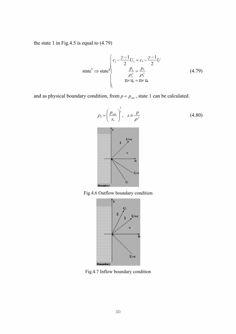
50

the state 1 in Fig.4.5 is equal to (4.79)

⎪⎪⎪

⎩

⎪⎪⎪

⎨

⎧

×=×

=

−−=

−−

⇒

*1

*

*

1

1

*11 21

21

statestate

unun

γγ ρρ

γγ

pp

UcUc

1* (4.79)

and as physical boundary condition, from outpp = , state 1 can be calculated.

γ

γ

ρρ ps

spout ≡⎟⎟

⎠

⎞⎜⎜⎝

⎛= ,

1

*1 (4.80)

Fig.4.6 Outflow boundary condition

Fig.4.7 Inflow boundary condition

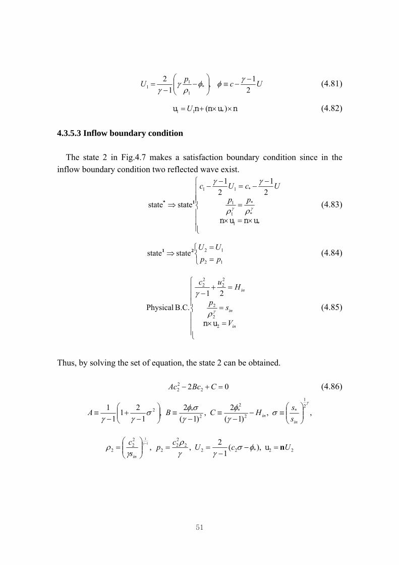
51

UcpU2

1,1

2*

1

11

−−≡⎟⎟

⎠

⎞⎜⎜⎝

⎛−

−=

γφφρ

γγ

(4.81)

nunnu ××+= )( *11 U (4.82)

4.3.5.3 Inflow boundary condition

The state 2 in Fig.4.7 makes a satisfaction boundary condition since in the inflow boundary condition two reflected wave exist.

⎪⎪⎪

⎩

⎪⎪⎪

⎨

⎧

×=×

=

−−=

−−

⇒

*1

*

*

1

1

*11 21

21

statestate

unun

γγ ρρ

γγ

pp

UcUc

1* (4.83)

⎩⎨⎧

==

⇒12

12statestateppUU21 (4.84)

⎪⎪⎪

⎩

⎪⎪⎪

⎨

⎧

=×

=

=+−

in

in

in

V

sp

Huc

2

2

2

22

22

21

B.C. Physical

un

γρ

γ

(4.85)

Thus, by solving the set of equation, the state 2 can be obtained.

02 222 =+− CBcAc (4.86)

,,)1(

2,)1(

2,1

211

1 21

*2

2*

2*2

γ

σγφ

γσφσ

γγ ⎟⎟⎠

⎞⎜⎜⎝

⎛≡−

−≡

−≡⎟⎟

⎠

⎞⎜⎜⎝

⎛−

+−

≡in

in ssHCBA

22*222

22

2

22

2 ),(1

2,,11

UcUcpsc

in

n=−−

==⎟⎟⎠

⎞⎜⎜⎝

⎛=

−

uφσγγ

ργ

ρ γ

52

4.3.6 Time integration In general, the method to discretize unsteady term exists two. These methods can be divided into two large classes: explicit and implicit methods. In brief, explicit methods calculate the state of a system at a later time from the state of the system at the current time. This method have some merits for the calculation per one step but it is considerably limited by Courant number. On the contrary, an implicit method finds it by solving an equation involving both the current state of the system and the later one and it is not the limitation of Courant number. Thus, this method can take comparatively big time step. As simple example, if Y(t) is the current system state and Y(t+Δt) is the state at the later time (Δt is a small time step), then, for an explicit method,

Y(t+Δt) = F(Y(t))

while for an implicit method one solves an equation, G(Y(t), Y(t+Δt)) = 0

to fine Y(t+Δt). In UPACS code, the methods for time integration are useful of following three

methods; Euler explicit method, Runge-Kutta (third order) method (Jameson-Baker, Jameson) and implicit method by using MFGS (Matrix Free Gauss-Seidel) (E. Shima, 1997). Of these three methods, Euler’s implicit method by using MFGS(Matrix Free Gauss-Seidel) method for time integration in this study is applied under consideration of calculation conditions.

1st order Euler’s implicit method - The estimation of Flux is carried out in next time step, n+1. Thus, in order to satisfy,

0)QQ( 11 =+− ∑ ++ dAFdtV nnn

sub-iteration per time step is carried out. At this time, however, the number of sub-iteration is made a decision depending on its objective. In getting steady solution, it must be 1.

2nd order Euler’s implicit method

53

- Flux is estimated by variable in next time step, n+1 like 1st order Euler’s implicit method and that in before time step, n-1 as follows

0)Q5.0Q2Q5.1( 111 =++− ∑ +−+ dAFdtV nnnn

Thus, this method is necessary to reserve variable in before time step, n-1 when the solutions in each time step are reserved.

4.4 Turbulence Model

This chapter provides details about the turbulence model available in this study. At first, turbulent flows are characterized by fluctuating velocity fields. These fluctuations mix transported quantities such as momentum, energy, and species concentration, and cause the transported quantities to fluctuate as well. Since these fluctuations can be of small and high frequency, they are too computationally expensive to simulate directly in practical engineering calculations. Instead, the instantaneous governing equations can be time-averaged, ensemble-averaged, or otherwise manipulated to remove the small scales, resulting in a modified set of equations that are computationally less expensive to solve. However, the modified equations contain additional unknown variables, and turbulence models are needed to determine these variables in terms of known quantities.

Turbulence model can be sorted as three different methods. In the below, information about these is described. 1. RANS (Reynolds averaged Navier-Stokes equations) This equation represents transport equations for the mean flow quantities

only, with all the scales of the turbulence being modeled. The approach of permitting a solution for the mean flow variables greatly reduces the computational effort. If the mean flow is steady, the governing equations will not contain time derivatives and a steady state solution can be obtained economically. A computational advantage is seen even in transient situations, since the time step will be determined by the global unsteadiness in the mean flow rather than by the turbulence. The Reynolds-averaged approach is generally adopted for practical engineering calculations, and uses models such

54

as Bladwin-Lomax, Spalart-Allmaras, k-ε and the RSM (Reynolds Stress Model).

2. LES (Large Eddy Simulation)

LES provides an alternative approach in which the large eddies are computed in a time-dependent simulation that uses a set of filtered equations. Filtering is essentially a manipulation of the exact Navier-Stokes equations to remove only the eddies that are smaller than the size of the filter, which is usually taken as the mesh size. Like Reynolds averaging, the filtering process creates additional unknown terms that must be modeled in order to achieve closure. Statistics of the mean flow quantities, which are generally of most engineering interest, are gathered during the time-dependent simulation. The attraction of LES is that, by modeling less of the turbulence, the error induced by the turbulence model will be reduced. One might also argue that it ought to be easier to find a universal model for the small scales, which tend to be more isotropic and less affected by the macroscopic flow features than the large eddies.

3. DNS (Direct Numerical Simulation)

This simulation doesn’t use the averaging method such as before two turbulence models. Thus, it is not needed the process to be modeled in simulation. Instead, the grids of the Kolmogorov scale, which regards as the smallest one in fluid flow simulation is needed for simulation. Therefore, the cost for simulation is substantially demanded, for especially three dimensional and unsteady flows. Until now, this simulation method is limited for simple phenomenon.

Under the information of turbulence models, the choice of turbulence model is very important issue in simulating the fluid flow. In this study, the Reynolds averaged Navier-Stokes model (the Spalart-Allmaras turbulence model) which is well known as comparatively simple method is used under the conditions and objectives considered. 4.4.1 Reynolds averaging

55

In Reynolds averaging, the solution variables in the instantaneous Navier-Stokes equations are decomposed into the mean and fluctuating components. For the velocity components,

′+= iii uuu (4.87)

where ūi and ui are the mean and instantaneous velocity component. Likewise, for pressure and other scalar quantities,

φφφ ′+= (4.89)

where φ denotes a scalar such as pressure and energy etc. Substitution expressions of this form for the flow variables into the instantaneous continuity and momentum equations and taking a time average (dropping the overbar on the mean velocity) yields the averaged momentum equations. They can be written in Cartesian tensor form as follows,

)3,2,1,(0)( ==∂∂

+∂∂ jiu

xt ii

ρρ (4.89)

)(32 ′′−

∂∂

+⎥⎥⎦

⎤

⎢⎢⎣

⎡⎟⎟⎠

⎞⎜⎜⎝

⎛

∂∂

−∂∂

+∂∂

∂∂

+∂∂

−= jijl

lij

i

j

j

i

ji

i uuxx

uxu

xu

xxDtDu ρδμρρ (4.90)

Eq.(4.89) and (4.90) are called Reynolds averaged Navier-Stokes (RANS) equations. They have the same general form as the instantaneous Navier-Stokes equations, with the velocities and other solution variables now representing time-averaged values. Additional terms now appear that represent the effects of turbulence. These Reynolds stresses, ′′− ji uuρ must be modeled in order to close (4.90) 4.4.2 Boussinesq approach

The Reynolds-averaged approach to turbulence modeling requires that the Reynolds stresses in (4.90) be appropriately modeled. A common method employs the Boussinesq hypothesis to relate the Reynolds stresses to the mean velocity gradients,

56

iji

it

i

j

j

itji x

ukxu

xuuu δμρμρ ⎟⎟

⎠

⎞⎜⎜⎝

⎛∂∂

+−⎟⎟⎠

⎞⎜⎜⎝

⎛

∂

∂+

∂∂

=′′−32 (4.91)

The Boussinesq hypothesis (Hinze, 1975) is used in the Reynolds averaged Navier-Stokes equations such as Bladwin-Lomax, Spalart-Allmaras and k-ε model. The advantage of this approach is the relatively low computational cost associated with the computation of the turbulent viscosity, μt. In the case of the Spalart-Allmaras model, only one additional transport equation which is represented turbulent viscosity is solved. In many cases, models based on this Boussinesq hypothesis perform very well. 4.4.3 The Spalart-Allmaras model

The Spalart-Allmaras model (Spalart and Allmaras, 1992) is a relatively simple one-equation turbulence model that solves a modeled transport equation for the kinematic eddy (turbulent) viscosity. This embodies a relatively new kind of one-equation turbulence model in which it is not necessary to calculate a length scale related to the local shear layer thickness. Thus, this turbulent model is applied for aerospace applications involving wall-bounded flows and has been shown to give good results for boundary layers subjected to adverse pressure gradients. It is also gaining popularity for turbo-machinery applications.

In turbulence models that employ the Boussinesq approach, the central issue is how the eddy viscosity is computed. The model used in this study proposed by Spalart and Allmaras solves a transport equation for a quantity that is a modified form of the turbulent kinematic viscosity. 4.4.3.1 Transport equation for the Spalart-Allmaras model

The transported variable in the Spalart-Allmaras model, ν~ is identical to the turbulent kinematic viscosity except in the near-wall region. The transport equation for ν~ is as follows,

57

( ) νν

ννρννρμ

σνρ Y

xC

xxG

DtD

jb

jj

−⎥⎥⎦

⎤

⎢⎢⎣

⎡

⎟⎟⎠

⎞⎜⎜⎝

⎛

∂∂

+⎪⎭

⎪⎬⎫

⎪⎩

⎪⎨⎧

∂∂

+∂∂

+=2

2~

~~~1~ (4.91)

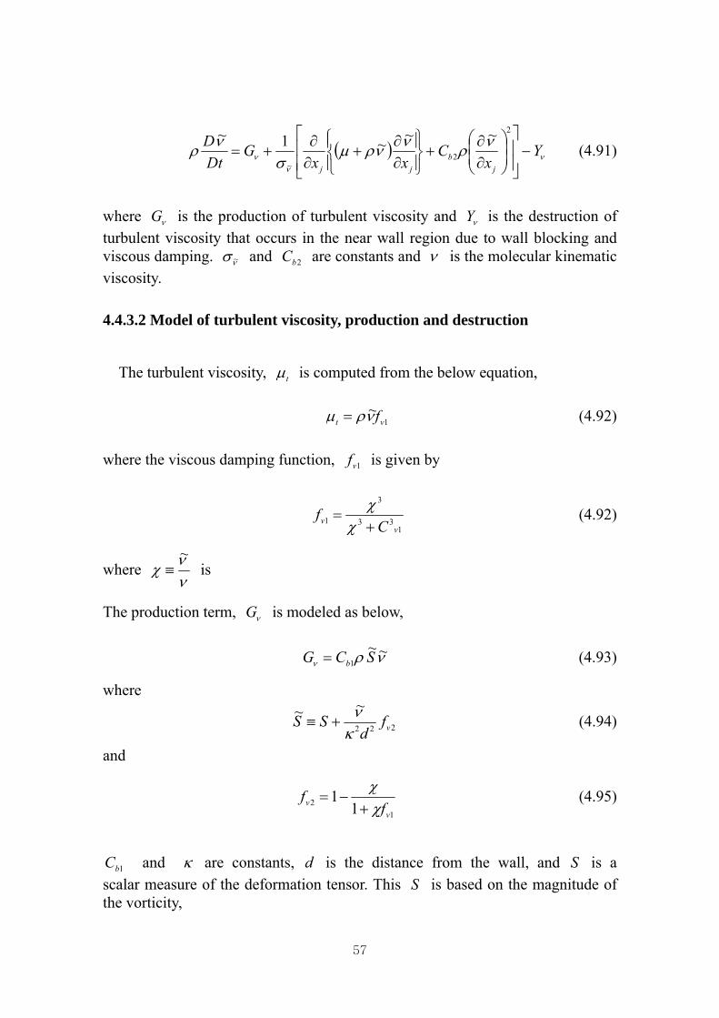
where νG is the production of turbulent viscosity and νY is the destruction of turbulent viscosity that occurs in the near wall region due to wall blocking and viscous damping. νσ ~ and 2bC are constants and ν is the molecular kinematic viscosity. 4.4.3.2 Model of turbulent viscosity, production and destruction

The turbulent viscosity, tμ is computed from the below equation,

1~

vt fνρμ = (4.92)

where the viscous damping function, 1vf is given by

133

3

1v

v Cf

+=χ

χ (4.92)

where ννχ~

≡ is

The production term, νG is modeled as below,

νρν~~

1 SCG b= (4.93)

where

222

~~vfd

SSκν

+≡ (4.94)

and

12 1

1v

v ff

χχ

+−= (4.95)

1bC and κ are constants, d is the distance from the wall, and S is a

scalar measure of the deformation tensor. This S is based on the magnitude of the vorticity,

58

ijijS ΩΩ≡ 2 (4.96)

where ijΩ is the mean rate of rotation tensor and is defined by

⎟⎟⎠

⎞⎜⎜⎝

⎛

∂∂

−∂∂

=Ωj

i

i

jij x

uxu

21 (4.97)

Here, S means that turbulence is found only where vorticity is generated near walls for the wall bounded flows that were of most interest when the model was formulated. However, since it has been acknowledged that one should also take into account the effect of mean strain on the turbulence production and a modification to the model has been proposed by researchers and incorporated into the code used in this study. This modification combines measures of both rotation and strain tensors in the definition of S,

( )ijijprodij SCS Ω−+Ω≡ ,0min (4.98)

where prodC =2.0, ijijij ΩΩ≡Ω 2 and ijijij SSS 2≡ , respectively

with the mean strain rate, Sij is defined as follows,

⎟⎟⎠

⎞⎜⎜⎝

⎛

∂∂

+∂∂

=j

i

i

jij x

uxu

S21 (4.99)

Including both the rotation and strain tensors reduces the production of eddy viscosity and consequently reduces the eddy viscosity itself in regions where the measure of vorticity exceeds that of strain rate. One such example can be found in vortical flows, i.e., flow near the core of a vortex subjected to a pure rotation where turbulence is known to be suppressed. Including both the rotation and strain tensors more correctly accounts for the effects of rotation on turbulence. The destruction term is modeled as

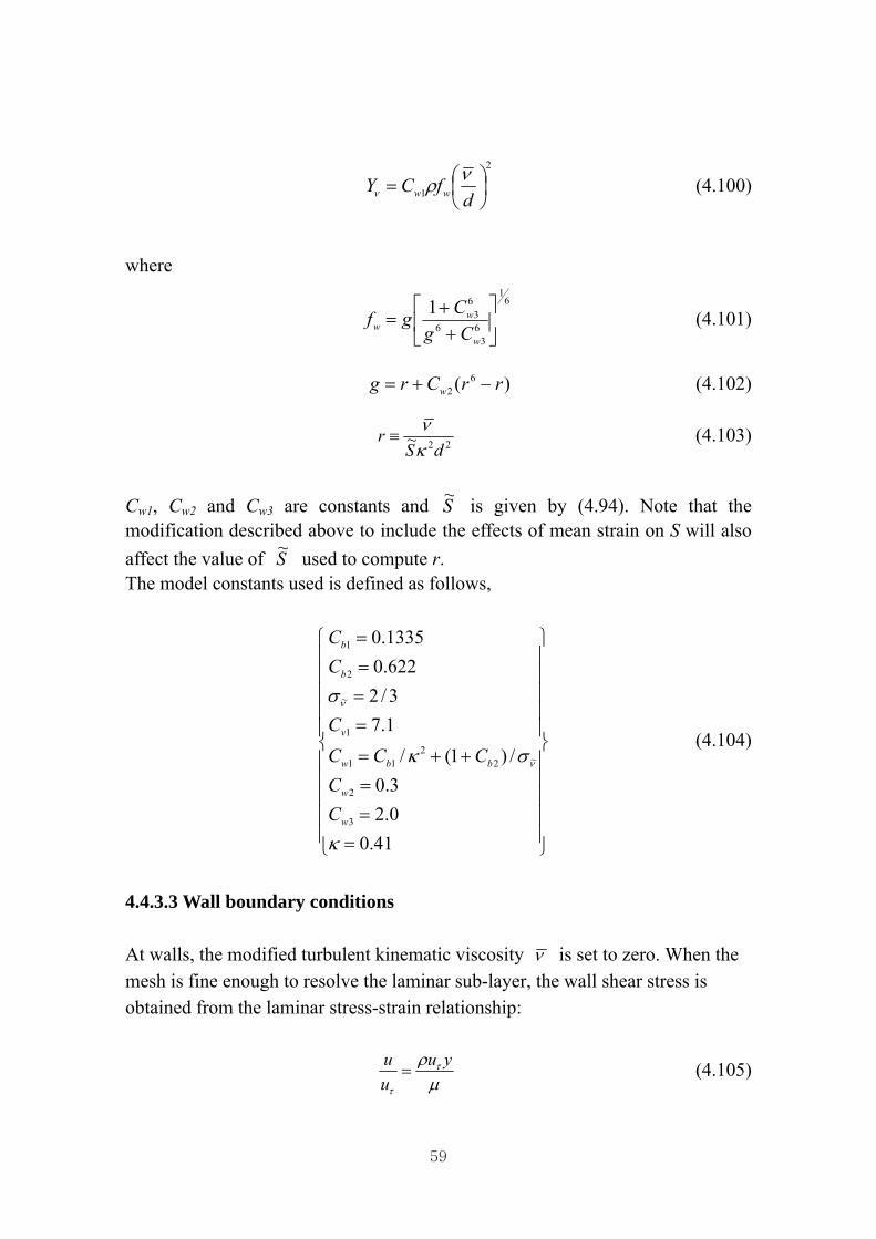
59

2

1 ⎟⎠⎞

⎜⎝⎛=

dfCY ww

νρν (4.100)

where

6

1

63

6

631⎥⎦

⎤⎢⎣

⎡++

=w

ww Cg

Cgf (4.101)

)( 62 rrCrg w −+= (4.102)

22~ dSr

κν

≡ (4.103)

Cw1, Cw2 and Cw3 are constants and S~ is given by (4.94). Note that the modification described above to include the effects of mean strain on S will also affect the value of S~ used to compute r. The model constants used is defined as follows,

⎪⎪⎪⎪⎪

⎭

⎪⎪⎪⎪⎪

⎬

⎫

⎪⎪⎪⎪⎪

⎩

⎪⎪⎪⎪⎪

⎨

⎧

===

++=

====

41.00.23.0

/)1(/1.73/2622.01335.0

3

2

~22

11

1

~

2

1

κ

σκ

σ

ν

ν

w

w

bbw

v

b

b

CC

CCCC

CC

(4.104)

4.4.3.3 Wall boundary conditions At walls, the modified turbulent kinematic viscosity ν is set to zero. When the mesh is fine enough to resolve the laminar sub-layer, the wall shear stress is obtained from the laminar stress-strain relationship:

μρ τ

τ

yuuu= (4.105)

60

If the mesh is too coarse to resolve the laminar sub-layer, it is assumed that the centroid of the wall-adjacent cell falls within the logarithmic region of the boundary layer, and the law-of-the-wall is employed:

)(ln1μ

ρ τ

τ

yuEku

u= (4.106)

where k=0.419 and E=9.793.

61

CHAPTER 5

THE EFFECT OF PRESSURE RATIO In this chapter, the comparison of the results by the experiment and computation is described. From this comparison, the validation of the computational code used in this study is confirmed. In addition, the self-generated mechanism of the spiral flow in the Conada nozzle from these results will be clarified. Finally, the flow features in the Coanda nozzle with the pressure ratio, po / pa = 1.11, 1.28 and 1.40 obtained from computational study are described.

5.1 Computational Conditions 5.1.1 Computational grids

The computational grids used in this study are shown in Fig.5.1 (a) and Fig.5.1 (b). Total domain including the Coanda nozzle for computation is selected such as Fig.5.1 (a) in order to minimize the affects by the surrounding boundary. Fig.5.1 (a) is the 2-dimensional grid system selected in the cross-section of total domain and Fig.5.1 (b) appears the 3-dimensional grid system in the nozzle part of total domains. The grids in the computational domain are selected after the grid refinement exercise. The total grid numbers used in the simulation is about 1,200,000 and the most grids is focused in the nozzle part relatively in order to obtain better results, especially in the buffer region, slit and wall surface in the nozzle and grid system is depending on structured grid. The UPACS code used in this study is based on the parallel computation as mention before. The parallel computation system is composed of 5 personal computers connected by a gigabyte network. The message passing interface (MPI) is used for implementing parallel processing. Thus, the total domain is divided into 27 blocks. Each block is equally assigned to 5 computers depending on grid size of it.

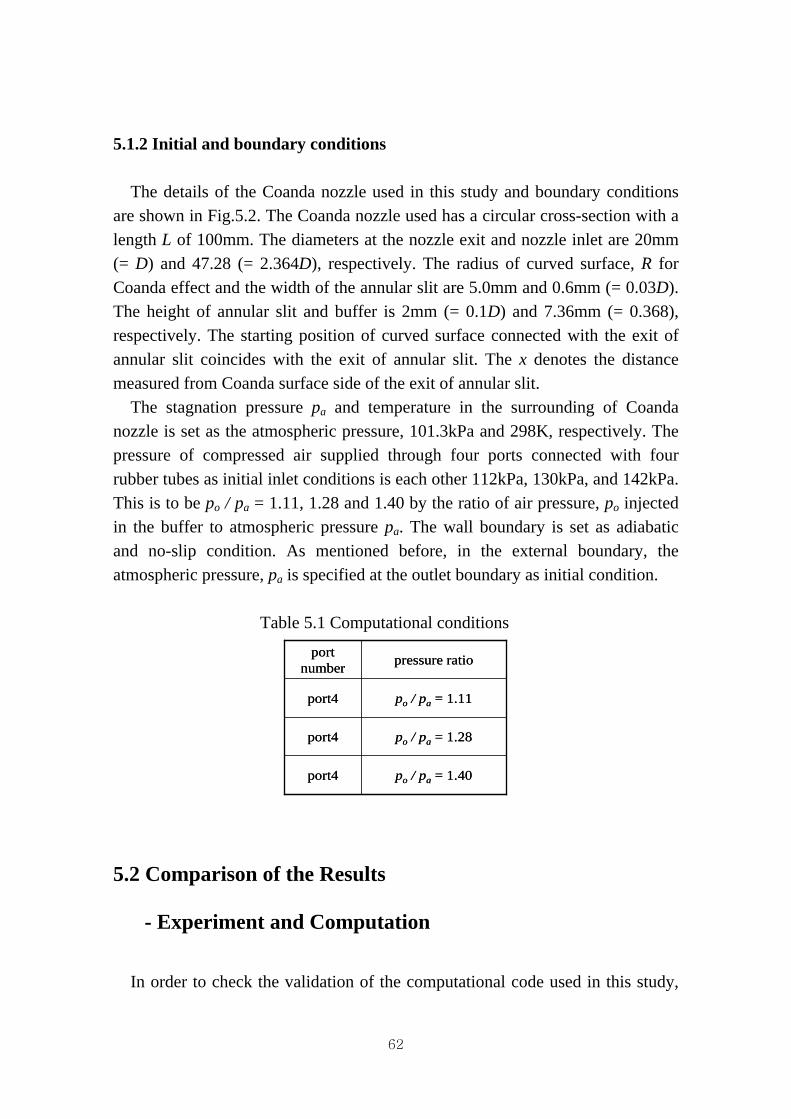
62

5.1.2 Initial and boundary conditions

The details of the Coanda nozzle used in this study and boundary conditions are shown in Fig.5.2. The Coanda nozzle used has a circular cross-section with a length L of 100mm. The diameters at the nozzle exit and nozzle inlet are 20mm (= D) and 47.28 (= 2.364D), respectively. The radius of curved surface, R for Coanda effect and the width of the annular slit are 5.0mm and 0.6mm (= 0.03D). The height of annular slit and buffer is 2mm (= 0.1D) and 7.36mm (= 0.368), respectively. The starting position of curved surface connected with the exit of annular slit coincides with the exit of annular slit. The x denotes the distance measured from Coanda surface side of the exit of annular slit.

The stagnation pressure pa and temperature in the surrounding of Coanda nozzle is set as the atmospheric pressure, 101.3kPa and 298K, respectively. The pressure of compressed air supplied through four ports connected with four rubber tubes as initial inlet conditions is each other 112kPa, 130kPa, and 142kPa. This is to be po / pa = 1.11, 1.28 and 1.40 by the ratio of air pressure, po injected in the buffer to atmospheric pressure pa. The wall boundary is set as adiabatic and no-slip condition. As mentioned before, in the external boundary, the atmospheric pressure, pa is specified at the outlet boundary as initial condition. Table 5.1 Computational conditions

po / pa = 1.40port4

po / pa = 1.28port4

po / pa = 1.11port4

pressure ratioport number

po / pa = 1.40port4

po / pa = 1.28port4

po / pa = 1.11port4

pressure ratioport number

5.2 Comparison of the Results

- Experiment and Computation

In order to check the validation of the computational code used in this study,

63

the comparison of the results by experiment and computation for pressure ratios, po / pa = 1.11 and 1.28 is carried out. Fig.5.3 and Fig.5.4 show the results for velocity distributions in the radial direction at the position of 10mm(x / D = 0.5) and 40mm(x / D = 2.0) respectively from the nozzle exit after the time proceeds enough.

In figures, the abscissa is the radial distance y measured from the nozzle centerline normalized to the diameter of the nozzle exit D, and the ordinate indicates non-dimensionalized values to the maximum axial and tangential velocity obtained by the experiment. A comparison between experimental and computational results for axial velocity distributions as shown in Fig.5.3 and Fig.5.4 shows satisfactory agreement, quantitatively and qualitatively. However, the difference in the axial velocity distributions at the distance x / D = 0.5 from nozzle exit is found. It can be thought as a result that the toughness of nozzle surface is not considered. Thus, the axial velocity flowing along internal wall of Coanda nozzle is over-expected compared with the values measured in the experiment. As a result, the development of the axial velocity on the centerline of the nozzle exit is relatively lagged. In general, in the case of swirl flow, it is well known that the turbulent intensity in the tangential direction compared with the axial direction is stronger. Therefore, it is confirmed that the better agreement in the axial velocity than in the tangential velocity from the results obtained is achieved. As expected, velocity distributions in both the experiment and computation in present position captured increase as the pressure ratios increase and the width of jet as the distance is getting bigger gradually by the transfer of momentum with environmental fluid.

5.3 Self-generating Mechanism of Spiral Flow

The compressed air supplied in the buffer by four rubber tubes from the reservoir tank collides with the bottom side of the buffer like the jet impinged with fixed wall. After this process, it propagates into the entire buffer region. It means that instantly the compressed air in the buffer has strong three dimensional flow features. Finally, it flows into Coanda nozzle through annular slit from the buffer.

Fig.5.5 shows the pressure contour in the cross-sectional side of the buffer

64

region with time. The pressure contour of the cross-sectional side at initial instant makes a balance through the entire buffer region by axis-symmetric structure of inlet ports of compressed air supplied from reservoir tank. However, as time passes, its flow has strong three dimensional flow features. As a result, the axis-symmetry of the pressure contour in the buffer region breaks down. It means that the flow state in the buffer region changes stable into unstable. This result is also confirmed apparently in the vector maps of the buffer region as shown in Fig.5.6.

Fig.5.7 and Fig.5.8 show the pressure contours and vector maps in the cross-sectional side of the buffer region including annular slit. As mentioned in Fig.5.5 and Fig.5.6, the results in this position also show same trend. The axis-symmetry in the pressure contours and vector maps in the buffer region disappears gradually as the time elapses.

At the instant, the air that goes through complicate flow process in the buffer region passes through narrow annular slit connected with the buffer and then flows out along internal wall surface of nozzle by the Coanda effect on the curved surface. In this process, it can be thought that the flow passing through annular slit from the buffer is almost predominant the normal velocity component to the exit of the annular slit. However, though its velocity magnitude is relatively very small to the normal velocity component, the tangential velocity component at the tip of annular slit is also detected by three dimensional flow characteristics and its instability in the buffer region with time. This result is showing in Fig.5.9. The tangential velocity component at the tip of annular slit makes considerably small deflection by the interaction between the normal (radial) velocity component and the axial velocity component developed by Coanda effect. As a result, the existence of relatively small tangential component detected in the exit of annular slit can be thought as the onset of the spiral flow with the turbulence of the normal velocity component at the exit of annular slit proposed by Horii etc.

However, the deflection near the nozzle exit which the radial and axial velocity component decrease increases relatively as shown in Fig.5.10 and Fig.5.11. As a result, the interaction between the tangential velocity component detected at the exit of annular slit and fast axial velocity component flowing along the internal wall surface of nozzle by the Coanda effect on the curvature surface connected with the tip of annular slit and its unique configuration like conical cylinder make a development into the spiral flow to have low swirl ratio and long rotating pitch. It is discriminant flow feature of spiral flow compared

65

with a conventional swirling jet. Fig.5.12 shows the vector maps at each position, x / D = 1.0, 2.0, 3.0 and 4.0.

As mentioned in the variation of velocity components along a streamline of Fig.5.10, the tangential velocity is defected at each position and its magnitude increases with the distance. It can also be explained by the theory of angular momentum conservation in swirl tube. Fig.5.13 appears the axial and tangential velocity distributions as the distance from the exit of nozzle. Since the reversed flow by the boundary layer between the induced flow and the primary flow from annular slit, the axial velocity distributions on the centerline of nozzle is not fully developed at the position of x / D = 0.5 from nozzle exit but in the position of x / D = 5.75, its velocity is fully recovered and has maximum value. As gone to downstream, the axial and tangential velocity distributions are expanded by the momentum loss with environmental flow.

5.4 The Effect of the Pressure Ratio The effect of the pressure ratio in axial velocity distributions

The flow passing through annular slit flows along internal wall surface by Coanda effect on the curved surface. At this time, the pressure near the exit of annular slit is relatively lower than that of nozzle inlet. The induced flow is dragged from nozzle inlet by this reason. The induced flow dragged by the difference of pressure makes a generation of a mixing layer with primary flow from annular slit. This mixing layer develops more and more in the downstream of nozzle and the stagnation point by the mixing layer is made in a position on nozzle centerline is finally stagnant. The induced flow around the centerline of Coanda nozzle is reversed in the upstream side by this stagnant region and in the downstream of stagnant point, the flow is accelerated by the conical configuration of nozzle. This process is shown well in Fig.5.14.

Fig.5.15 shows the axial velocity distributions on the centerline of nozzle with the increase of pressure ratio. In figure, the ordinate and abscissa appear the non-dimensionalized distance to the diameter of nozzle exit and axial velocity magnitude, respectively. As mentioned in Fig.5.14, the reversed flow is detected in the vicinity of the nozzle inlet for all pressure ratios and the velocity magnitude of the reversed flow here is getting higher as the pressure ratio

66

increases. The axial velocity on the centerline of nozzle in the downstream of a stagnant point generated by the boundary layer between the induced flow and the primary flow passing through the annular slit is recovered as goes to nozzle exit. However, unlike expected, the position of stagnation point is almost same for all pressure ratios in this study. This is due to the interaction by the induced flow from nozzle inlet and the primary flow from annular slit.

In the following, the axial velocity distributions at each position are shown in Fig.5.16. The fluid flowing along the curved surface is accelerated in here by Coanda effect and has relatively considerably high axial velocity. It is more apparent as the pressure ratio increases. On the contrary, the axial velocity distributions in the radial direction have larger velocity gradient as the pressure ratio increases. This is the result that the velocity magnitude of reversed flow and the acceleration of axial velocity on the curved surface increase with the pressure ratio. It can be explained by the flow rate from annular slit with the pressure ratio. However, the large gradient in axial velocity between the wall surface of nozzle and the center of nozzle decreases as goes to downstream of nozzle and the recovery of the axial velocity in the lowest pressure ratio is the fastest of all pressure ratios. The effect of the pressure ratio in tangential velocity distributions

The tangential velocity distributions detected at the tip of annular slit is shown in Fig.5.17. Its value increases as the pressure ratio increases. It can be considered that the flow state in the buffer region is to be more complicated and the flow instability in here increases with the increase of the pressure ratio. From the results obtained, the increase of the ratio of the stagnant pressure in the buffer region to that of atmospheric air means the increase of normal velocity to the surface of annular slit and tangential velocity detected at the tip of annular slit. As mentioned before, it can be taken into account as the onset of spiral flow to have self-generating tangential component in Coanda nozzle and has an important relation with the tangential velocity component observed inside and outside of nozzle.

The tangential velocity distributions in the nozzle in the case of pressure ratio, po / pa = 1.28 are shown in Fig.5.18. As shown before results, the tangential velocity components detected at the tip of annular slit by strong three dimensional flow features and the flow instability in the buffer region decrease relatively by the axial velocity accelerated by Coanda effect on the curved

67

surface, but by the nozzle configuration of conical cylinder type it increases again as goes to the exit of nozzle. This physical phenomenon is based on the conservation of the circulation at every point on a vortex tube. The vortex tube in the present flow structure of the annular jet is forced to contract towards the nozzle axis. The contraction results in an increase of tangential velocity satisfying the principle of circulation conservation. Thus, it is clearly clarified for all cases to have same nozzle configuration. In addition, the forced vortex region and the free vortex region are also confirmed in the present study like those by Horii’s theoretical analysis (1991). The maximum vorticity is found in the neighborhood of central axis. It means the converging vortex is generated in and leads to the focusing of the spiral flow jet.

In order to investigate the relation of velocity components in Coanda nozzle, the variation of velocity components obtained along a streamline from the buffer to nozzle exit is shown in Fig.5.19. In the variation of velocity components obtained from a streamline, axial and tangential velocity components go through three flow process (acceleration, deceleration and acceleration process) by the Coanda effect on the curved surface and nozzle configuration of conical cylinder type. Radial velocity component has high value in the vicinity of the tip of annular slit, but as shown in general conical nozzle, its value decreases gradually as goes to the downstream of nozzle. The flow characteristics outside nozzle as the pressure ratio

Fig.5.20 and Fig.5.21 show the axial and tangential velocity distributions at the position of x / D = 0.5 and 2.0, respectively. The abscissa is non-dimensionalized distance in radial direction to the diameter of nozzle exit and the ordinate is non-dimensionalized value to have maximum axial and tangential velocity components obtained at each position for the pressure ratio, po / pa = 1.28. The axial and tangential velocity distributions at each position increases as the pressure ratio increases. The increase of the pressure ratio means that of the flow rate exhausted from annular slit. It is equal to the increase of axial velocity passing through Coanda nozzle and the tangential velocity detected at the tip of annular slit as mentioned before. As a result, the axial and tangential velocity distributions at the position of x / D = 0.5 and 2.0 increase with the pressure ratio. The difference in the axial velocity around internal wall and the centerline of nozzle is still sustained to the position, x / D = 0.5 from nozzle exit. However, it is almost recovered for the first time at the position, x / D = 2.0.

68

In addition, the jet width is getting wider and wider by the momentum transfer with environmental fluid.

The ratio of maximum tangential velocity, Vθmax to maximum axial velocity, Vxmax in the distance, x / D = 0.5 and 2.0 from nozzle exit with pressure ratio is shown in Fig.5.22. From now on, it is denoted as the swirl intensity of spiral flow in present study. In Fig.5.22, the abscissa and ordinate are the swirl intensity and pressure ratio, respectively. As the pressure ratio increases, it is observed that the swirl intensity increases in both positions. This trend is approximately linear and the swirl intensity for all cases decreases a little with the distance. From these results, in the present study, it can be thought that the decay in the axial velocity with the distance from nozzle exit is smaller than that in the tangential velocity. It is the reason that the spiral flow has a high focusing ability compared with normal jets and conventional swirling jets as mentioned by Horii et al (1991). In addition, the scale of the decay in swirl intensity is the biggest in the case of pressure ratio, po / pa = 1.11 and the smallest in the case of pressure ratio, po / pa = 1.40.

69

5.5 Summary In this chapter, the validation of computational code used in this study was checked through the comparison of the results by the experiment and computation. Based on these results, the self-generated mechanism of the spiral flow in Coanda nozzle was apparently clarified and the flow characteristics in Coanda nozzle with the increase of the pressure ratio were described. The results obtained from these are as following; 1) The compressed air supplied through four rubber tubes is propagated into

entire buffer region and then it has axisymmetric features. But as time passes, it breaks by the flow instability and has asymmetric and three dimensional flow features.

2) In the flow exhausted from annular slit passing through the buffer region, normal velocity component to the surface of annular slit is almost predominant, but the tangential velocity component at the tip of annular slit with it is also detected. It can be thought as the onset of the spiral flow in Coanda nozzle.

3) The unique configuration of Coanda nozzle play a key role in sustaining the momentum of the flow exhausted from annular slit. In other words, though the configuration of Conada nozzle helps radial momentum decrease, it sustains or increases the axial and tangential momentum through nozzle.

4) The increase of pressure ratio means that of the flow rate exhausted from annular slit. The tangential velocity distributions detected at the tip of annular slit and the axial velocity on the curvature surface increase by it.

5) The magnitude of reversed flow in axial velocity on the centerline of nozzle increases with the pressure ratio. On the contrary, the development of axial velocity in the downstream of stagnant point by the growth of the boundary between the induced flow and the primary flow from annular slit is faster with the pressure ratio.

6) The axial and tangential velocity obtained at the appointed position from nozzle exit increase as the pressure ratio does. This trend has a close relation with the tangential velocity distributions at the tip of annular slit with the pressure ratio.

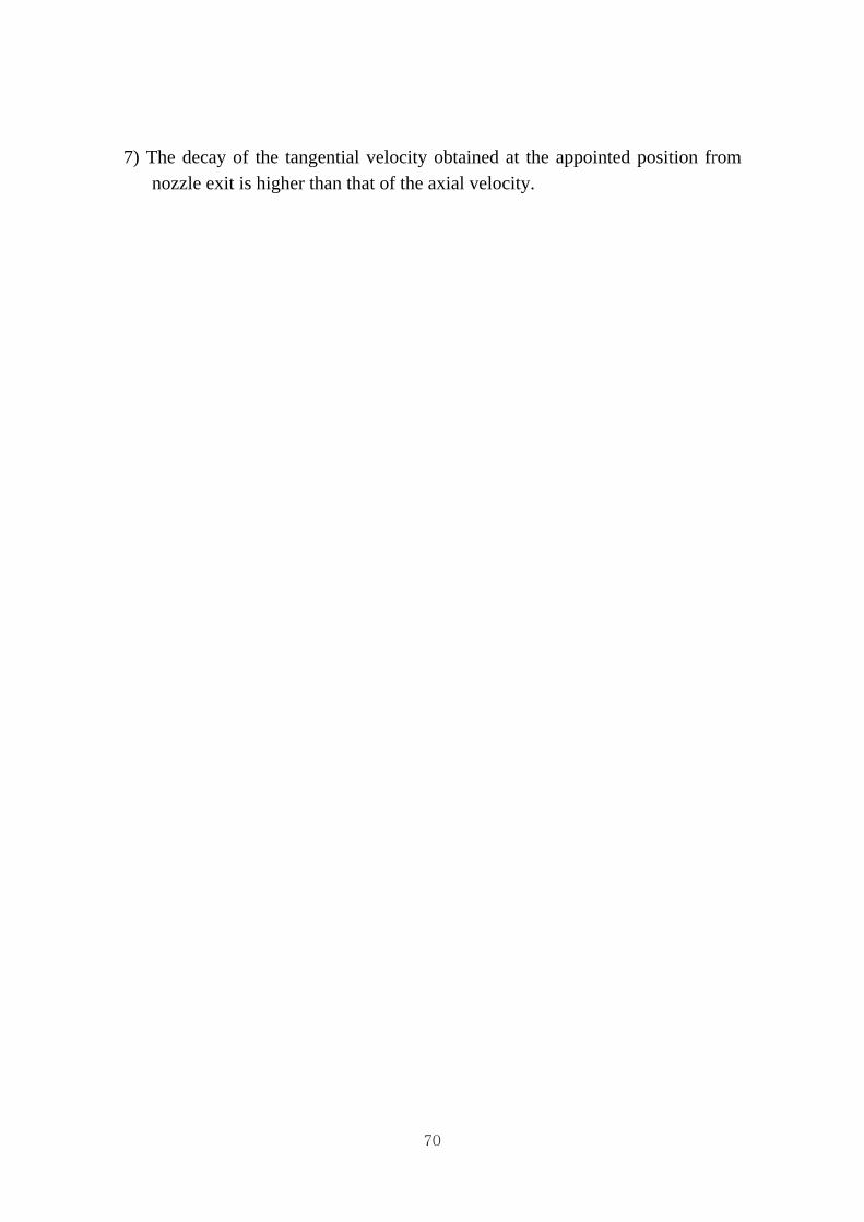
70

7) The decay of the tangential velocity obtained at the appointed position from nozzle exit is higher than that of the axial velocity.

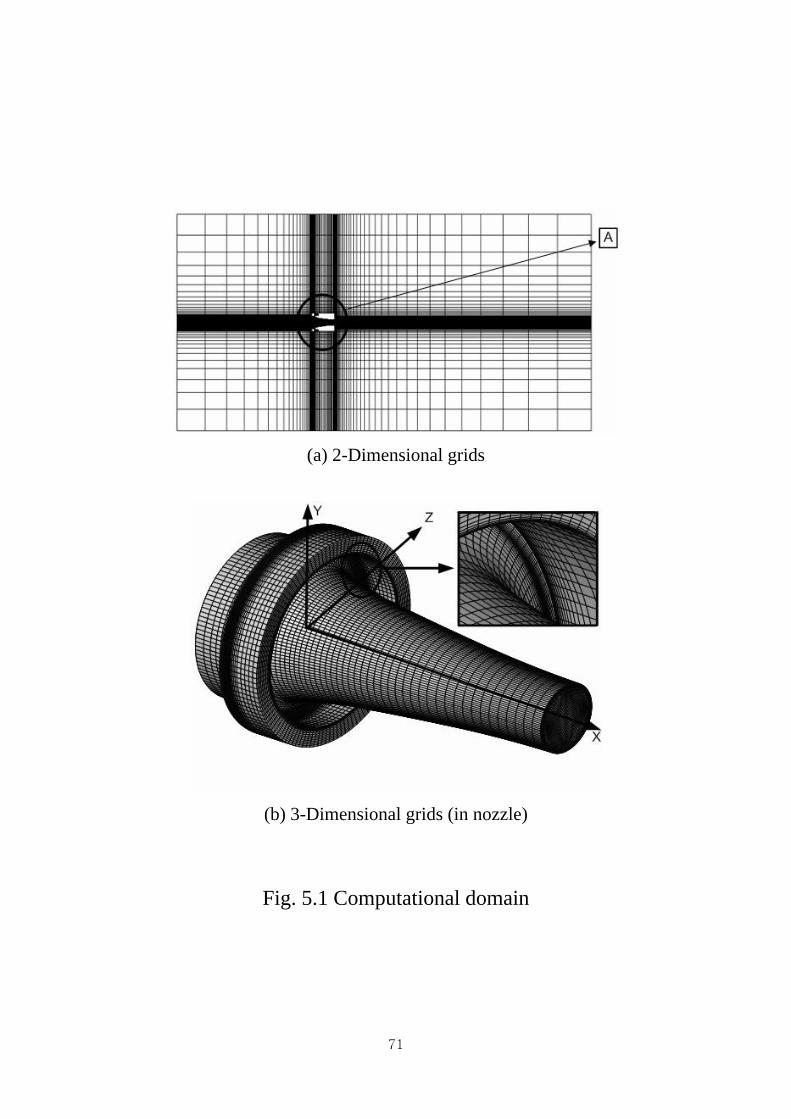
71

(a) 2-Dimensional grids

(b) 3-Dimensional grids (in nozzle)

Fig. 5.1 Computational domain

72

Fig. 5.2 Nozzle configuration and boundary conditions

73

(a) Axial velocity distributions

(b) Tangential velocity distributions

Fig. 5.3 Velocity distributions in the radial direction at the

position of x / D = 0.5 (from nozzle exit)

74

(a) Axial velocity distributions

(b) Tangential velocity distributions

Fig. 5.4 Velocity distributions in the radial direction at the

position of x / D = 2.0 (from nozzle exit)

75

Fig.5.5Variations of pressure contour in the buffer region with time

76

Fig.5.6 Variations of vector maps in the buffer region with time

77

Fig.5.7 Variations of pressure contour in the cross-section of annular slit with time

78

Fig.5.8 Variations of vector maps in the cross-section of annular slit with time

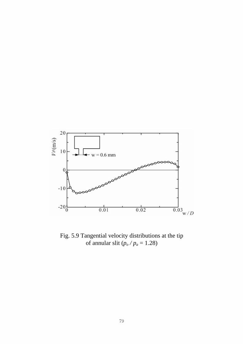
79

Fig. 5.9 Tangential velocity distributions at the tip of annular slit (po / pa = 1.28)

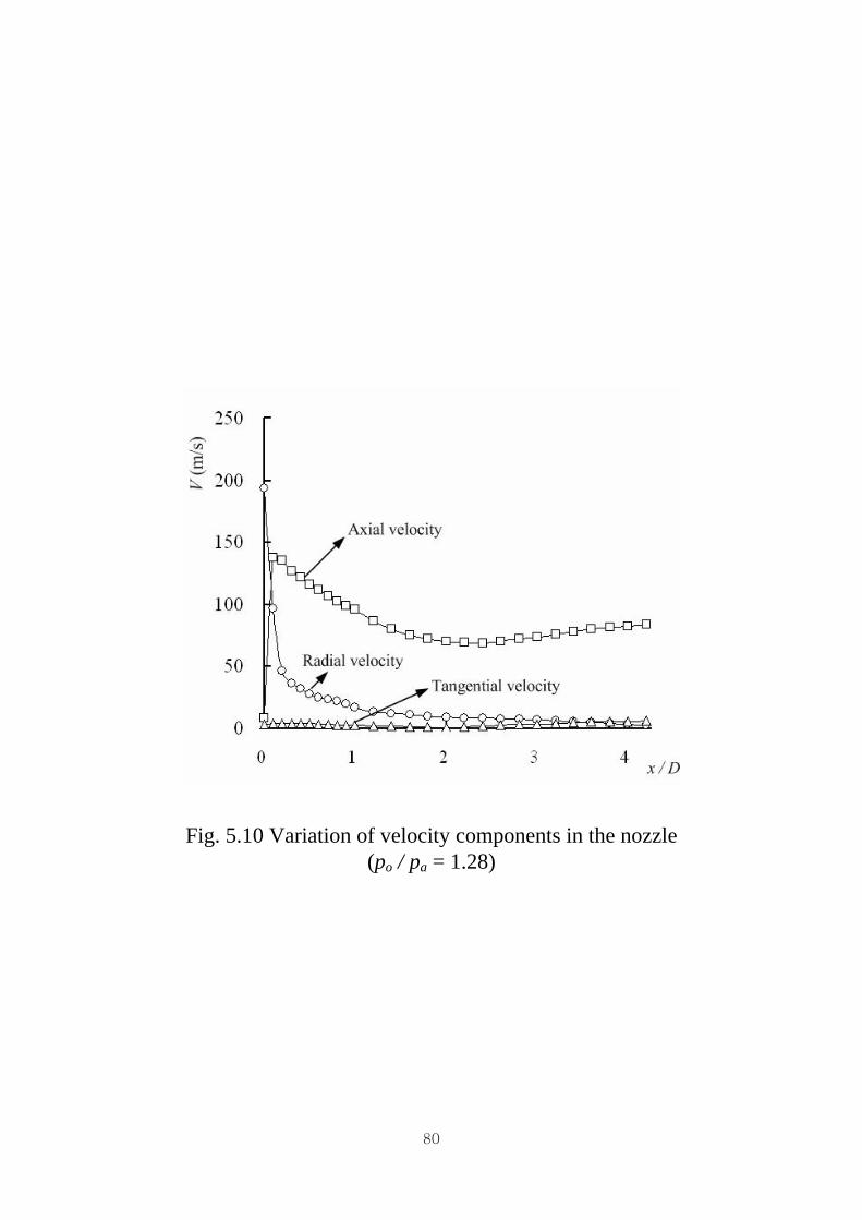
80

Fig. 5.10 Variation of velocity components in the nozzle (po / pa = 1.28)

81

(a) Sketch of spiral flow

(b) The transition of streamlines through nozzle

Fig. 5.11 The generation of spiral flow in the nozzle

82

Fig. 5.12 Vector maps at each position of nozzle

83

(a) Axial velocity distributions in radial direction (from nozzle exit)

(b) Tangential velocity distributions in radial direction (from nozzle exit) Fig. 5.13 Velocity distributions with the distance from nozzle exit

(po / pa = 1.28)

84

Fig. 5.14 The transition of streamlines in Coanda Nozzle

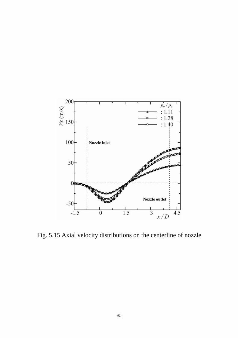
85

Fig. 5.15 Axial velocity distributions on the centerline of nozzle

86

Fig. 5.16 Axial velocity distributions in the nozzle

87

Fig. 5.17 Tangential velocity distributions at the tip of annular slit

88

Fig. 5.18 Tangential velocity distributions in the nozzle

(po / pa = 1.28)

89

(a) Variation of axial velocity along a streamline

(b) Variation of radial velocity along a streamline

(c) Variation of tangential velocity along a streamline

Fig. 5.19 Variation of velocity components along a streamline

90

(a) Axial velocity distributions

(b) Tangential velocity distributions

Fig. 5.20 Velocity distributions at the position of x / D = 0.5

91

(a) Axial velocity distributions

(b) Tangential velocity distributions

Fig. 5.21 Velocity distributions at the position of x / D = 2.0

92

(a) x / D = 0.5 (from nozzle exit)

(b) x / D = 2.0 (from nozzle exit)

Fig. 5.22 Swirl intensity

93

CHAPTER 6

THE EFFECT OF NOZZLE GEOMETRY

6.1 Computational Conditions 6.1.1 Computational grids

The computational grids used in this study are shown in Fig.6.1.1 (a) and Fig.6.1.1 (b). The entire domain including Coanda nozzle for computation is selected such as Fig.6.1.1 (a) in order to minimize the affects by the surrounding boundary. Fig.6.1.1 (a) is the 2-dimensional grid system selected in the cross-section of total domain and Fig.6.1.1 (b) displays the 3-dimensional grid system in the nozzle part of total domain. The grid system in present computational domain is selected after the grid refinement exercise. The total grid numbers used in the simulation is about 1,200,000 in the study for the change of slit width and slit angle and 800,000 for the change of the geometry of nozzle inlet, respectively. The most grids is focused in the nozzle part relatively in order to obtain better results, especially in the buffer region, annular slit and near wall surface in the nozzle. The UPACS code used in this study is based on the parallel computation as mention before. The parallel computation system is composed of 5 personal computers connected by a gigabyte network. The message passing interface (MPI) is used for implementing parallel processing. Thus, the total domain is divided into 18 and 27 blocks for each computational condition. Each block is equally assigned to 5 computers depending on grid size of it. 6.1.2 Initial and boundary conditions

The stagnation pressure pa and temperature in the surrounding of Coanda nozzle is set as the atmospheric pressure, 101.3kPa and 298K, respectively. The pressure of compressed air supplied through four ports connected with four rubber tubes as initial inlet conditions is 130kPa. This is to be po / pa = 1.28 by the ratio of air pressure, po injected in the buffer to atmospheric pressure pa. This

94

initial condition is equally applied for all cases described in this chapter. The wall boundary is set as adiabatic and no-slip condition. As mentioned before, in the external boundary, the atmospheric pressure, pa is specified at the outlet boundary as initial condition.

6.2 The Effect of the Width of Annular Slit 6.2.1 Details of nozzle configuration

In this section, in order to understand the effect of the width of annular slit on the flow features, its width is only changed from 0.2mm (= 0.01D) to 0.6mm (= 0.03D). Fig.6.2.1 shows the details of this configuration. However, the basic configuration of Coanda nozzle including the height of annular slit, the curvature surface connected with annular slit and the size of buffer region that plays a role in generation of the spiral flow in this unique nozzle is fixed. The computational conditions for present study are tabulated in Table 6.2.1.

Table 6.2.1 Computational conditions for the change of slit width

0.6mmpo / pa = 1.28port4

0.4mmpo / pa = 1.28port4

0.2mmpo / pa = 1.28port4

Slit widthPressure ratioPort

number

0.6mmpo / pa = 1.28port4

0.4mmpo / pa = 1.28port4

0.2mmpo / pa = 1.28port4

Slit widthPressure ratioPort

number

6.2.2 Effect of the width of annular slit on the flow features

The axial velocity distributions on the centerline of the nozzle with the change of slit width are showing in Fig.6.2.2. In this figure, the abscissa is non-dimensionalized distance in axial direction to the diameter of the exit of nozzle and the ordinate is the axial velocity obtained on the centerline of Coanda nozzle. The position of stagnant point by the boundary growth between the induced flow from the inlet of nozzle and the primary flow injected from annular slit is almost

95

equal for all cases. However, the magnitude of reverse flow in the upstream of stagnant point is the highest in the slit width, w=0.6mm (= 0.03D). On the contrary, the slit width, w=0.2mm (= 0.01D) has the lowest value in its magnitude. The position of maximum reverse flow moves to near the inlet of nozzle as the width of annular slit is getting wider. It can be expected to have a relation with the induced flow sucked from the inlet of nozzle. In other words, the increase of slit width means the increase of flow rate exhausted from annular slit and it also does the increase of the difference in the pressure between the inlet of nozzle and near annular slit. By the difference in the pressure at two positions the secondary flow is dragged. Its magnitude also increases with the slit width. As a result, the reversed flow reflected by the boundary layer between the induced flow and the primary flow is also high velocity value.

Fig.6.2.3 shows axial velocity distributions in the radial direction at each position of nozzle. The abscissa and ordinate is normalized to the diameter of nozzle exit. As shown in Fig.6.2.2, the stagnant point is found between x / D = 1.0 and 2.0. The area of reversed flow is wider as the slit width. The axial velocity of the primary flow flowing along the curvature surface by Coanda effect has the highest value in the case of the slit width, w=0.6mm. Thus, the axial velocity gradient between near the wall surface and near the centerline of nozzle in this case is considerably high in comparison of other cases. However, this gradient in axial velocity is recovered as goes to the exit of nozzle.

Fig.6.2.4 shows the tangential velocity distributions detected at the tip of annular slit. The tangential velocity in the region is found for all cases and its magnitude is the highest in the slit width, w=0.6mm. Since the existence of the tangential velocity in this region is regarded as an onset of the generation of the spiral flow in the Coanda nozzle, the potential of the detection of tangential velocity component can be expected inside and outside of nozzle.

In order to understand the decay of velocity components in axial and tangential direction, the velocity distributions are obtained at an appointed position. These results are shown in Fig.6.2.5 and Fig.6.2.6. At the position of x / D = 0.5 from nozzle exit, the axial velocity distributions is not same with the change of slit width. It can be presumed that though pressure ratio is equal for all cases, the flow rate exhausted from annular slit passing through the buffer region is the most in the case of the slit width, w=0.6mm by the difference of slit width. It is the reason to have different velocity distributions at current position. With the distance to the downstream, the jet width is getting wider by the momentum

96

transfer with environmental air in the boundary layer and at the position of x / D = 2.0, the axial velocity on the centerline is entirely developed relatively. This is a different feature in comparison of conventional swirling flow. The decay in axial and tangential velocity is confirmed. However, its decay is more apparent in the tangential velocity distribution than in the axial velocity distribution. Fig.6.2.7 shows the ratio of maximum tangential velocity to maximum axial velocity, Vθmax / Vx max obtained at each position. As the slit width increases, this value increases. However, the decay of this value in the cases of the slit width, w=0.2 and w=0.4mm at the position of x / D = 2.0 is apparent in comparison of the case of the slit width, w=0.6mm. As mentioned before, it is the result that the decay in the tangential velocity in the case of the slit width, w=0.6mm has relatively little decay than that in other two cases.

6.3 The Effect of the Inclination Angle of Annular Slit 6.3.1 Details of nozzle configuration

In order to investigate the effect for the change of the inclination angle of annular slit, the annular slit of Coanda nozzle is only changed from 0o to 30o as shown in Fig.6.3.1. However, the basic configuration of Coanda nozzle including the height of annular slit, the curvature surface connected with annular slit and the size of buffer region that plays a role in generation of the spiral flow in this unique nozzle is fixed as shown in before study. As explained, initial and boundary condition is equal to those in the section 6.1.2. The computational conditions in present study are tabulated in Table 6.3.1.

Table 6.3.1 Computational conditions for the change of slit width

30opo / pa = 1.28port4

15opo / pa = 1.28port4

0opo / pa = 1.28port4

Inclination angle of annular slitPressure ratio

Portnumber

30opo / pa = 1.28port4

15opo / pa = 1.28port4

0opo / pa = 1.28port4

Inclination angle of annular slitPressure ratio

Portnumber

97

6.3.2 Effect of the inclination angle of annular slit on the flow features

The axial velocity distributions on the centerline of the nozzle with the change of slit width are showing in Fig.6.3.2. In this figure, the abscissa is non-dimensioned value of the distance in axial direction to the diameter of nozzle exit and the ordinate is the axial velocity obtained on the centerline of Coanda nozzle. The position of stagnant point by the growth of boundary layer between the induced flow from the inlet of nozzle and the primary flow injected from annular slit is almost equal for all cases. In addition, the magnitude of reverse flow in the upstream of stagnant point is almost equal regardless of the inclination angle of annular slit. The position which the maximum velocity of reversed flow is detected is almost equal and it exists between x / D = 0 and 1.

Fig.6.3.3 shows axial velocity distributions in the radial direction at each position of nozzle. The abscissa and ordinate is normalized to the diameter of nozzle exit. As shown in Fig.6.3.3, it is confirmed that the axial velocity obtained at the tip of annular slit have more or less big value with the increase in the inclination angle of annular slit. It means that the inclination angle of annular slit has an influence on the fluid issued from annular slit. On the contrary, the tangential velocity at the tip of annular slit is the highest in the case of the inclination angle of annular slit, θ=0o. This result can confirm in Fig.6.3.4 which represents the tangential velocity distributions at the tip of annular slit.

In order to understand the velocity distributions for axial and tangential direction in the downstream of the exit of nozzle, the velocity distributions are obtained an appointed position. These results are shown in Fig.6.3.5 and Fig.6.3.6. At the position of x / D = 0.5 from nozzle exit, the axial velocity distributions doesn’t show high difference with the change of the inclination angle of annular slit. It can be presumed by the results for velocity distributions obtained in Coanda nozzle. Although the tangential velocity at the tip of annular slit for the case not to have the inclination angle of annular slit is the highest in comparison of other cases, the tangential velocity distributions obtained at the appointed position from the exit of nozzle have big value in the order of the magnitude of the inclination angle unlike expectation. It means that the velocity components related with the generation of the spiral flow in Coanda nozzle is not only the axial and tangential velocity component. In other words, the radial velocity component also plays a role in the generation of the spiral flow.

In the tangential velocity distributions from nozzle exit, the region of forced

98

vortex increases gradually with increasing the inclination angle of annular slit. Fig.6.3.7 shows the ratio of maximum tangential velocity to maximum axial

velocity, Vθmax / Vxmax obtained at each position. Based on the results obtained from Fig.6.3.5 and Fig.6.3.6, the increase of the inclination angle of annular slit can expect the increase of the ratio of maximum tangential velocity to maximum axial velocity, Vθmax / Vxmax obtained at each position. The decay of Vθmax / Vxmax

with the distance from nozzle exit is the highest in the case of the inclination angle, θ=30o. It implies that the case of the inclination angle, θ=30o which of these three cases has the highest angular momentum has the strongest momentum transfer with environmental fluid.

6.4 The Effect of Nozzle Inlet Geometry 6.4.1 Details of nozzle configuration

In fact, the induced flow occurred by the pressure difference has an influence on the flow features in Coanda nozzle. In this section, the effect for open or closed type of nozzle inlet is investigated. Fig.6.4.1 shows details of the configuration in these cases. Case 1 is open and the distance from nozzle inlet to annular slit is 15mm (=0.75D) and Case 2 and Case 3 is closed and the distance is 15mm (=0.75D) and 7.5mm (=0.375D), respectively. However, the basic configuration of Coanda nozzle including the height of annular slit, the curvature surface connected with annular slit and the size of buffer region that plays a role in generation of the spiral flow in this unique nozzle is fixed. The computational conditions are tabulated in Table 6.4.1.

Table 6.4.1 Computational conditions for the change of inlet geometry

Closed

Closed

Open

Type of nozzle inlet

0.375D

0.75D

0.75D

Distance between nozzle inletand annular slit (L)

po / pa = 1.28port4

po / pa = 1.28port4

po / pa = 1.28port4

Pressure ratioPort

number

Closed

Closed

Open

Type of nozzle inlet

0.375D

0.75D

0.75D

Distance between nozzle inletand annular slit (L)

po / pa = 1.28port4

po / pa = 1.28port4

po / pa = 1.28port4

Pressure ratioPort

number

99

6.4.2 Effect of nozzle inlet geometry on the flow features

The axial velocity distributions on the centerline of the nozzle with the change of slit width are showing in Fig.6.4.2. In this figure, the abscissa is non-dimensioned distance in axial direction to the diameter of the exit of nozzle and the ordinate is the axial velocity obtained on the centerline of Coanda nozzle. The stagnant point by the boundary growth of the primary flow exhausted from annular slit is confirmed on the centerline of nozzle. Its position moves to downstream of nozzle as shown in Fig.6.4.2. It is more apparent in the cases of Case 2 and Case 3 not to have the induced flow from nozzle inlet. Case 2 and Case 3, which have the closed structure in the configuration of nozzle inlet, have higher reversed flow velocity than Case 1. It is reflected to rear surface and the reflected flow has an influence on the boundary layer resulted from the primary flow. Finally, this reflected flow makes the boundary layer by the primary flow move to downstream of nozzle. It is the reason that the position of stagnant point of Case 2 and Case 3 is positioned in the downstream than Case 1. This result is also appeared well in Fig.6.4.3.

As mentioned, the existence of tangential velocity component at the tip of annular slit is very important for the spiral flow self-generated in Coanda nozzle since it can be thought as the onset of the spiral flow in it. The tangential velocity distributions at the tip of annular slit is confirmed for all cases as shown in Fig.6.4.4. Its magnitude is higher in Case 2 and Case 3 than in Case 1. By these results, the deflection angle of streamline, in other words, the maximum tangential velocity inside and outside of nozzle can be presumed is higher in Case 2 and Case 3 than in Case 1.

Fig.6.4.5 and Fig.6.4.6 show the axial and tangential velocity distribution at the position of x / D = 0.5 and 2.0 from nozzle exit. In each figure, the abscissa is non-dimensioned distance in axial direction to the diameter of the exit of nozzle and the ordinate is the value non-dimensioned to the maximum axial and tangential velocity obtained from Case 1 at the position of x / D = 0.5. For the axial velocity distributions of Fig.6.4.5 (a) and Fig.6.4.6 (a), Case 1 which the flow rate by the induced flow is increased, has faster axial velocity than Case 2 and Case 3 for each position as expected. But the retardation of the axial velocity distributions around the centerline is also very apparent of three cases. For the tangential velocity distributions of Fig.6.4.5 (b) and Fig.6.4.6 (b), the tangential velocity in Case 2 and Case 3 based on the results as shown in Fig.6.4.4 has

100

relatively high velocity distributions in comparison of Case 1. Based on the velocity distributions at the position of x / D = 0.5 and 2.0 from

nozzle exit, the ratio of maximum tangential velocity to maximum axial velocity Vθmax / Vxmax is obtained. Fig.6.4.7 shows this result about it. From the results, Case 1 which has relatively low initial tangential velocity is almost the decay of the tangential velocity to the axial velocity in current position, while Case 2 and Case 3 is bigger decay in the tangential velocity than that in the axial velocity. As the nozzle inlet is opened or closed, the flow features in Coanda nozzle have many variations. Especially, the region of free vortex in the cases of closed type is smaller than that of open type. However, the difference for the flow features with the distance between rear wall and annular slit when the nozzle inlet is closed is almost not confirmed. It implies that in the case of closed type, the effect with the distance between rear wall and annular slit is not existed.

101

6.5 Summary In this chapter, the flow features on the change of the configuration of Coanda nozzle; the width and inclination angle of annular, and the geometry of nozzle inlet, is investigated. The results obtained from these are as following; The effect of the width of annular slit 1) As the width of annular slit increases, the recirculation region is getting wider

in upstream of stagnant point and the axial velocity magnitude of reversed flow on the centerline of nozzle increases. And the position which it is found moves to nozzle inlet.

2) The increase of the slit width means that of the flow rate for the fluid exhausted from annular slit and the axial and tangential velocity obtaining in the nozzle increase by the increase of the flow rate with the width of annular slit.

3) The axial velocity distributions near the internal wall and the center of nozzle has high gradient around the annular slit but its gradient is recovered as goes to the downstream of stagnation point.

4) The tangential velocity distributions obtained at the tip of annular slit has an influence on that obtained at nozzle exit. Both values increased as the width of annular slit increases.

5) The decay in the ratio of maximum tangential velocity to maximum axial velocity at each position, x / D = 0.5, 2.0 from nozzle exit is the biggest in S.W. = 0.2mm and smallest in S.W. = 0.6mm in present conditions.

The effect of the inclination angle of annular slit 1) As the inclination angle of annular slit increases, the recirculation region is

getting wider in upstream of stagnant point but its difference is not so big since the difference of the flow rate exhausted from annular slit with the inclination angle is very small.

2) The axial velocity component at the tip of annular slit is obtained by the change of the configuration of annular slit. Its value increases with the inclination angle. However, since the present radius of curvature surface for Coanda effect is fixed, the flow between the tip of annular slit and curvature

102

surface is very complicate. As a result, the variation of axial velocity in this region increases.

3) The tangential velocity distributions at the tip of annular slit with the Inclination angle is the biggest in S.A. = 0o, while the magnitude of the tangential velocity obtained from nozzle exit is the smallest in it unlike expected. This can be thought that although the tangential velocity distributions at the tip by the inclination of annular slit is decreased, it has not an influence on the magnitude of the tangential velocity detected from nozzle exit.

4) The decay in the ratio of maximum tangential velocity to maximum axial velocity at each position, x / D = 0.5, 2.0 from nozzle exit is the biggest in the inclination angle of annular slit, S.A. = 30o.

The effect of nozzle inlet geometry 1) As with or without induced flow, the stagnation point on the centerline moves

to downstream of nozzle. It is since the reflected flow to rear wall has an influence on the development of boundary layer.

2) In case of without induced flow, the magnitude of the axial velocity of reversed flow is almost same regardless of the distance between rear wall of nozzle and annular slit.

3) The axial velocity gradient between near internal wall surface and centerline of nozzle in the Case 2 and Case 3 in comparison of Case 1 is little. It means that the recovery of the axial velocity on the centerline is faster in the cases of Case 2 and Case3.

4) Based on the tangential velocity distributions at the tip of annular slit and the axial velocity distributions in the nozzle, Case 1 in the axial velocity has higher than Case 2 and Case 3 but in the tangential velocity, Case 2 and Case 3 have higher value than Case 1.

103

(a) 2-Dimensional grids

(b) 3-Dimensional grids (in nozzle)

Fig. 6.1.1 Computational domain

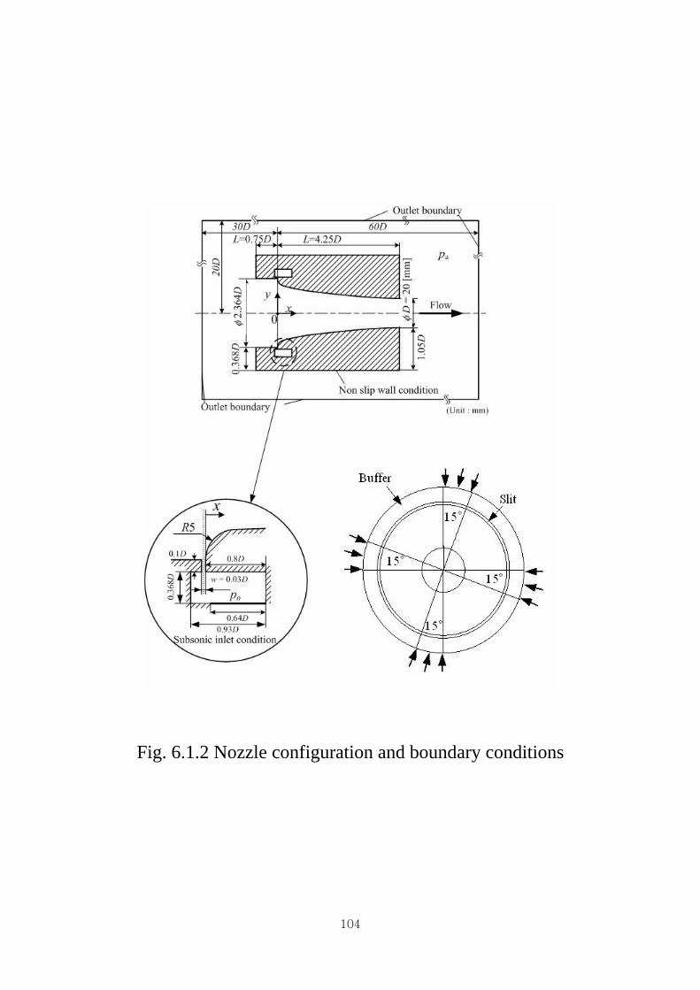
104

Fig. 6.1.2 Nozzle configuration and boundary conditions

105

Fig. 6.2.1 Details of the configuration of annular slit

Fig. 6.2.2 Axial velocity distributions on the centerline of the

nozzle with the width of annular slit (mm)

106

Fig. 6.2.3 Axial velocity distributions in the nozzle

107

Fig. 6.2.4 Tangential velocity distributions at the tip of annular slit

108

(a) Axial velocity distributions

(b) Tangential velocity distributions

Fig. 6.2.5 Velocity distribution at the position of x / D = 0.5

109

(a) Axial velocity distributions

(b) Tangential velocity distributions

Fig. 6.2.6 Velocity distributions at the position of x / D = 2.0

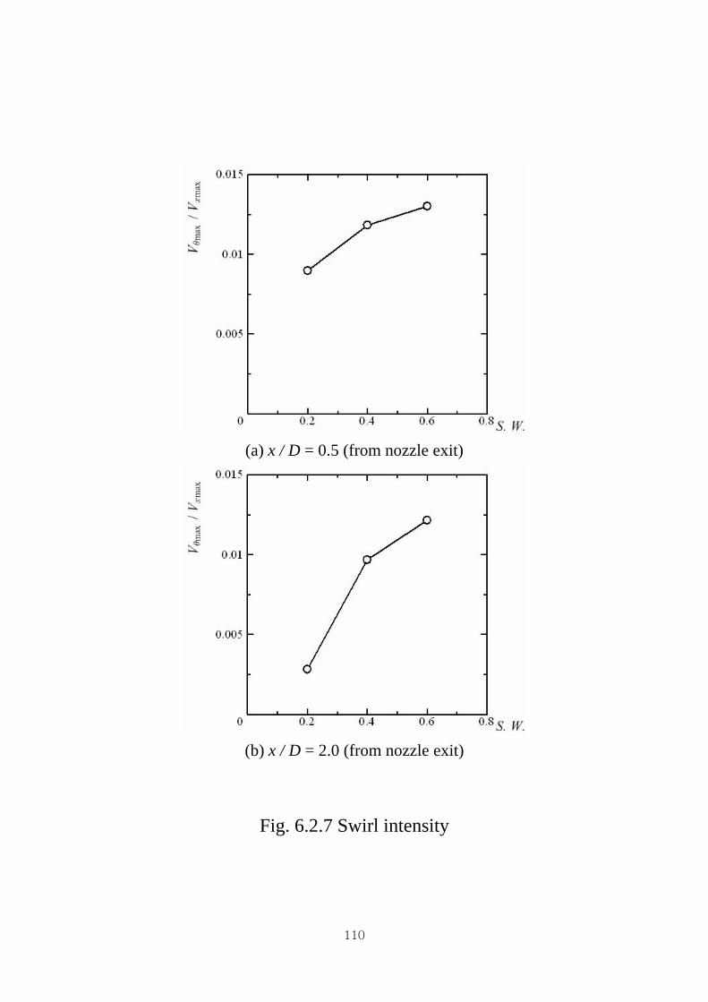
110

(a) x / D = 0.5 (from nozzle exit)

(b) x / D = 2.0 (from nozzle exit)

Fig. 6.2.7 Swirl intensity

111

Fig. 6.3.1 Details of the configuration of annular slit

112

Fig. 6.3.2 Axial velocity distributions on the centerline of the nozzle with the inclination angle

113

Fig.6.3.3 Axial velocity distributions in the nozzle

114

Fig. 6.3.4 Tangential velocity distributions at the tip of annular slit with the inclination angle

115

(a) Axial velocity distributions

(b) Tangential velocity distributions

Fig. 6.3.5 Velocity distributions at x / D = 0.5 from nozzle exit

116

(a) Axial velocity distributions

(b) Tangential velocity distributions

Fig. 6.3.6 Velocity distributions at x / D = 2.0 from nozzle exit

117

(a) x / D = 0.5 (from nozzle exit)

(b) x / D = 2.0 (from nozzle exit)

Fig. 6.3.7 Swirl intensity

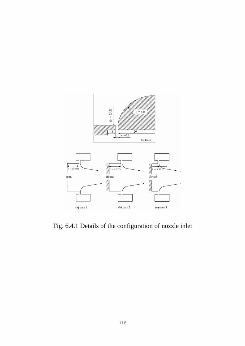
118

Fig. 6.4.1 Details of the configuration of nozzle inlet

119

Fig. 6.4.2 Axial velocity distributions on the centerline of the nozzle with the change of inlet geometry

120

Fig. 6.4.3 Axial velocity distributions in the nozzle

121

Fig. 6.4.4 Tangential velocity distributions at the tip of annular slit with the inlet geometry of nozzle

122

(a) Axial velocity distributions

0 (b) Tangential velocity distributions

Fig. 6.4.5 Velocity distribution at the position of x / D = 0.5

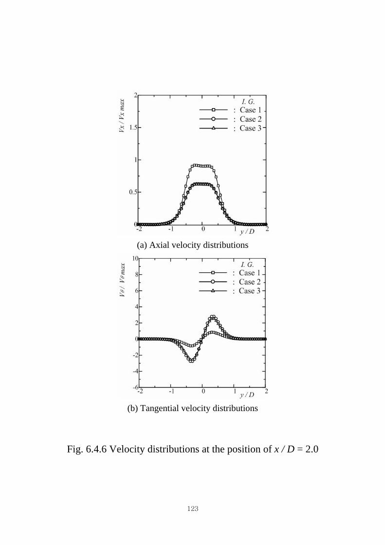
123

(a) Axial velocity distributions

(b) Tangential velocity distributions

Fig. 6.4.6 Velocity distributions at the position of x / D = 2.0

124

(a) x / D = 0.5 (from nozzle exit)

(b) x / D = 2.0 (from nozzle exit)

Fig. 6.4.7 Swirl intensity

125

CHAPTER 7

CONCLUSIONS The present study describes an experimental and computational work to propose the self-generating mechanism of the spiral flow in Coanda nozzle and to investigate the flow characteristics by the pressure ratio and the change of the configuration of Coanda nozzle. The results obtained from these works are summarized; The effect of the pressure ratio 1) The compressed air supplied through four rubber tubes is propagated into

entire buffer region and then it has axisymmetric features. But as time passes, it breaks by the flow instability and has asymmetric and three dimensional flow features.

2) In the flow exhausted from annular slit passing through the buffer region, normal velocity component to the surface of annular slit is almost predominant, but the tangential velocity component at the tip of annular slit with it is also detected. It can be thought as the onset of the spiral flow in Coanda nozzle.

3) The unique configuration of Coanda nozzle play a key role in sustaining the momentum of the flow exhausted from annular slit. In other words, though the configuration of Conada nozzle helps radial momentum decrease, it sustains or increases the axial and tangential momentum through nozzle.

4) The increase of pressure ratio means that of the flow rate exhausted from annular slit. The tangential velocity distributions detected at the tip of annular slit and the axial velocity on the curvature surface increase by it.

5) The magnitude of reversed flow in axial velocity on the centerline of nozzle increases with the pressure ratio. On the contrary, the development of axial velocity in the downstream of stagnant point by the growth of the boundary between the induced flow and the primary flow from annular slit is faster with the pressure ratio.

6) The axial and tangential velocity obtained at the appointed position from nozzle exit increase as the pressure ratio does. This trend has a close relation

126

with the tangential velocity distributions at the tip of annular slit with the pressure ratio.

7) The decay of the tangential velocity obtained at the appointed position from nozzle exit is higher than that of the axial velocity.

The effect of the width of annular slit 1) As the width of annular slit increases, the recirculation region is getting wider

in upstream of stagnant point and the axial velocity magnitude of reversed flow on the centerline of nozzle increases. And the position which it is found moves to nozzle inlet.

2) The increase of the slit width means that of the flow rate for the fluid exhausted from annular slit and the axial and tangential velocity obtaining in the nozzle increase by the increase of the flow rate with the width of annular slit.

3) The axial velocity distributions near the internal wall and the center of nozzle has high gradient around the annular slit but its gradient is recovered as goes to the downstream of stagnation point.

4) The tangential velocity distributions obtained at the tip of annular slit has an influence on that obtained at nozzle exit. Both values increased as the width of annular slit increases.

5) The decay in the ratio of maximum tangential velocity to maximum axial velocity at each position, x / D = 0.5, 2.0 from nozzle exit is the biggest in S.W. = 0.2mm and smallest in S.W. = 0.6mm in present conditions.

The effect of the inclination angle of annular slit 1) As the inclination angle of annular slit increases, the recirculation region is

getting wider in upstream of stagnant point but its difference is not so big since the difference of the flow rate exhausted from annular slit with the inclination angle is very small.

2) The axial velocity component at the tip of annular slit is obtained by the change of the configuration of annular slit. Its value increases with the inclination angle. However, since the present radius of curvature surface for Coanda effect is fixed, the flow between the tip of annular slit and curvature surface is very complicate. As a result, the variation of axial velocity in this

127

region increases. 3) The tangential velocity distributions at the tip of annular slit with the

Inclination angle is the biggest in S.A. = 0o, while the magnitude of the tangential velocity obtained from nozzle exit is the smallest in it unlike expected. This can be thought that although the tangential velocity distributions at the tip by the inclination of annular slit is decreased, it has not an influence on the magnitude of the tangential velocity detected from nozzle exit.

4) The decay in the ratio of maximum tangential velocity to maximum axial velocity at each position, x / D = 0.5, 2.0 from nozzle exit is the biggest in the inclination angle of annular slit, S.A. = 30o.

The effect of nozzle inlet geometry 1) As with or without induced flow, the stagnation point on the centerline moves

to downstream of nozzle. It is since the reflected flow to rear wall has an influence on the development of boundary layer.

2) In case of without induced flow, the magnitude of the axial velocity of reversed flow is almost same regardless of the distance between rear walls of nozzle and annular slit.

3) The axial velocity gradient between near internal wall surface and centerline of nozzle in the Case 2 and Case 3 in comparison of Case 1 is little. It means that the recovery of the axial velocity on the centerline is faster in the cases of Case 2 and Case3.

4) Based on the tangential velocity distributions at the tip of annular slit and the axial velocity distributions in the nozzle, Case 1 in the axial velocity has higher than Case 2 and Case 3 but in the tangential velocity, Case 2 and Case 3 have higher value than Case 1.

128

REFERENCE [1] R.-H. Chen, S. B. Saadani and L. P. Chew, “Effect of Nozzle on Screech Noise

Elimination from Swirling Underexpanded Jets”, Journal of Sound and Vibration, Vol. 252(1), pp. 178-186 (2002).

[2] R. Neemeh, S. Algattus and L. Neemeh, “Experimental Investigation of Noise

Reduction in Supersonic Jets due to Jet Rotation”, J. of Sound and Vibration, Vol. 221(3), pp. 505-524 (1999).

[3] M. Ameri, “An Experimental and Theoretical Study of Coanda Ejectors”, Ph.D

thesis, Case Western Reserve University (1993). [4] UPACS Ver. 1.5 Manual, JAXA [5] M. Vanierschot and E. Van den Bulck, “Numerical study of hysteresis in

annular swirling jets with a stepped-conical nozzle”, Int’l Journal for Numerical Methods in Fluids, Nov. 2006.

[6] J. C. CHEN AND C. A. LIN, “Computations of Strongly Swirling Flows”, Int.

J. Numer. Mech. Fluids, Vol.30, pp.493-508 (1999). [7] Norman A. Phillips, “An Explication of the Coriolis Effect”, Bulletin of the

American Meteorological Society, Vol.81, No.2, pp.299-303 (2000). [8] Horii, K., Matsumae, Y., Cheng, X. M., Takei, M. and Yasukawa, E., Focusing

Phenomena and Stability of Spiral-Flow Jet, Trans. Japan Soc. Aero. Space Sci., 33- 102, pp.141-153 (1991).

[9] Takei, M., Horii, K., Hashimoto, B., Kataoka, I., Ito, H. and Matsumae, Y.,

High Stability of Spiral Jet – Relations between Axial Velocity Distribution and Stability, J. of the Japan Soc. for Aeronautical and Space Sciences, 43-494, 9-16(1995).

[10] Miyazaki, K., Chen, G., Kudamatsuo, J., Sugimoto, T., Yamamoto, F. and

Horii, K., High-Efficiency Soil Transportation with Spiral Airflow, Japan Soc. Aero. Space Sci., 42-137, pp.105-111(1999).

[11] Ueda, H., Sakai, M., Horii, K., Funatsu, K. and Tomita, Y., Study of Swirling

Pneumatic Transport of Granule in a Horizontal Pipe, Trans. Jpn. Soc. Mech.Eng., 67-664, 3011-3017(2001).

129

[12] Horii, K., Sawazaki, H., Matsumae, Y., Cheng, X. M., Take, M., Yasukawa, E. and Hashimoto, B., New Continuous System for Dispersion and Encapsulation of Submicron Powders Using Spiral Flow, ASME-Industrial Application of Fluid Mechanics, Vol.FED-100, 25-30(1990).

[13] Takei, M., Horii, K., Hashimoto, B., Kataoka, I., Ito, H. and Matsumae, Y.,

Cutting of Soft Materials Using of Spiral Water Jet, J. of the Japan Soc. for Aeronautical and Space Sciences, 42-490, 36-47 (1994).

[14] Horii, K., Matsumae, Y., Ohsumi, K., Cheng, X. M., Kage, S. and Hashimoto,

B., Novel Optical Fiber Installation by Use of Spiral Flow, J. of Fluids Engineering, 114, 373-378 (1992).

[15] Horii, K., Matsumae, Y., Cheng, X. M., Takei, M. and Hashimoto, B., A

Study of Spiral Flow (Part 4) The Effect of Radial Reynolds Number of Spiral Flow on Plasma Deposition of Pipe, Trans. Japan Soc. Aero. Space Sci., 32-98, 165-175 (1990).

[16] Bhagwat, M. J., Leishman, J G., Correlation of Helicopter Rotor Tip Vortex

Measurements, AIAA Journal, 38(2), 301-308(2000). [17] Yamane, T, Yamamoto, K., Enomoto, S., Takaki, R., Tamazaki, H., Makida,

M., Tamamoto, T., Iwamiya, T. and Nakamura, T., Current Status of Common CFD Platform – UPACS, Proc. of Aerospace Numerical Simulation Symposium 2000, 45-50 (2000).

[18] Spalart, P. R. and Allmaras, S. R., “A one-equation turbulence model for

aerodynamics flows”, AIAA paper 92-0439, (1992). [19] Kim, T. H., Matsuo, S., Setoguchi, T. and Kim, H. D., “Study of Spiral Flow

Generated through an Annualr Slit”, Int. J. of Turbo & Jet-Engines, Vol.14, No.2, 97-102 (2005).

[20] S. V. Alekseenko, P. A. Kuibin, V. L. Okulov and S. I. Shtork, “Helical

vortices in swirl flow”, J. of Fluid Mech., Vol. 32, pp. 195-243(1999). [21] M. Garcia-Villalba, J. Frohlich and W. Rodi, “Unsteady phenomena in an

unconfined annular swirling jet”, Proc. of 10th European Turbulence Conference (2004).

[22] GIBSON, M.M. and YOUNIS, B.A., “Calculation of swirling jets with a

Reynolds stress closure”, Phys. of Fluids, Vol.29, 1, pp.38(1986).

130

[23] H. D. Kim, G. Rajesh, T. Setoguchi and S. Matsuo, “Optimization study of a coanda ejector”, J. of Thermal Science, Vol. 15, No. 4, pp. 331-336(2006).

[24] S. Vladimir and H. Fazle, “Collapse, Symmetry, breaking, and hysteresis in

swirling flows”, J. of Fluid Mech., Vol. 31, pp. 537-566(1999). [25] S. Turguf, “Effect of the Adverse Pressure Gradient on Vortex Breakdown”,

AIAA Journal, Vol. 12, No. 5, pp. 602-607(1974). [26] S. Turgut, “Vortex Breakdown in Swirling Conical Flows”, AIAA Journal,

Vol. 9, No. 9, pp. 1792-1799(1971). [27] Frank Kreith and O. K. Sonju, “The decay of a turbulent swirl in a pipe”, J. of

Fluid Mech., Vol. 22, pp. 257-271(1965). [28] Cho, W. B., Kim, H. D., “ A Fundamental Study of the Subsonic Spiral Jet”,

Proceedings of KSME Fall Meeting, pp.502-507 (2003). [29] Cho, W. B. Baek, S. C. and Kim, H. D., “The Effect of Annular Slit on a

Compressible Spiral Jet Flow”, Proceedings of KSME Spring Meeting, pp.2029-2034 (2004).

[30] Cho, W. B., Baek, S. C. and Kim, H. D., “The Effect of Coanda Wall

Curvature on Spiral Jet,” The 3rd National Congress on Fluids Engineering, pp. 619-622 (2004).

[31] B. S. Baldwin and H. Lomax, “Thin layer approximation and algebraic model

for separated turbulent flows”, AIAA Paper 78-0257 (1978). [32] P. L. Roe, “Approximate rieman solvers, parameter vectors, and difference

schemes”, Journal of Computational Physics, Vol.43, pp.357-372 (1981). [33] Y. Wada and M. S. Liou, “An flux splitting scheme with high-resolution and

robustness for discontinuities”, AIAA Paper 94-0083, January (1994). [34] Y. Wada and M. S. Liou, “An accurate and robust flux splitting scheme for

shock and contact discontinuities”, SIAM Journal on Scientific and Statistical Computing, Vol.18, No.3, pp.633-657 (1997)

[35] C. Hirsh, “Numerical Computation of Internal and External

Flows(Computational Methods for Inviscid and Viscous Flows)”, John Wiley & Sons (1989).

131

[36] S. R. Chakravarthy and S. Osher, “Numerical experiments with the Osher upwind scheme for the euler equations”, AIAA Journal, Vol.21, No.9, September (1983).

[37] Weiss, J. M, Smith, W. A., “Preconditioning applied to variable and constant

density flows”, AIAA Journal, Vol.33, No.11, pp.2050-2057 (1995). [38] M. Sano, “Numerical Analysis of Turbulent Boundary Layers with Injection

and Suction through a Slit”, JSME International Journal, Vol.35, No.4, pp.479-485 (1992).

[39] T. Nishizawa, K. Funatsu, K. Horii, and Y. Tomita, “Characteristics of

turbulent swirling flow in a straight pipe”, Proceedings of JSME, No.948-3, pp. 194-196 (1994).

[40] H. D. Shin, “Turbulent Mixing in Swirling Flows”, Transactions of the KSAE,

Vol.9, No.5, pp.19-24 (1987). [41] S. Nemoda, V. Bakic, S. Oka, G. Zivkovic, and N. Crnomarkovic,

“Experimental and Numerical Investigation of Gaseous Fuel Combustion in Swirl Chamber”, Int. J. of Heat and Mass Transfer, Vol.48, pp. 4623-4632 (2005).

[42] P. Bradshaw, D. H. Ferriss and R. F. Johnson,“Turbulence in the noise-

producing region of a circular jet,” J. Fluid Mech., Vol.19, pp. 591-623 (1963).

[43] H. Katanoda, Y. Mizato, M. Masuda, and K. Matsuo, “Pitot pressure of

correctly-expanded and underexpanded free jets axisymmetric supersonic nozzles”, Shock Waves, Vol.10, No.2, pp.95-101 (2000).

[44] Matsumae, Y. et al., “Enhanced Optical Cable Installation using Spiral

Airflow”, ASME Forum on Industrial and Environmental Applications of Fluids Mechanics, FED-Vol.221, pp.39-43 (1995).

[45] Cheng, X. M. Y. et al., “The Rope Passing Method for Repair of

Petrochemical Pipeline with Spiral Flow”, Sekiyu Gakkaishi, Vol.35, pp.382-389 (1992).

[46] M. Freitag, M. Klein, M. Gregor, D. Geyer, C. Schneider, A. Dreizler, and J.

Janicka, “Mixing analysis of a swirling recirculating flow using DNS and experimental data,” Int. J. of Heat and Mass Transfer, (2006).

132

[47] M. Vanierschot and E. Van den Bulck, “Numerical study of hysteresis in annular swirling jets with a stepped-conical nozzle”, Int. J. Numer. Meth. Fluids (2006).

[48] D. L. Young, C. B. Liao, and H. J. Sheen, “Computation of Recirculation

Zones of a Confined Annular Swirling Flow”, Int. J. Numer. Meth. Fluids, Vol.29, pp.791-810 (1999).

[49] M. Garcia-Villalba, J. Frohlich, and W. Rodi, “Unsteady phenomena in an

unconfined annular swirling jet”, Proceedings of the 10th European Turbulence Conference, Barcelona 2004.

[50] Y. C. Chao, J. H. Leu, and Y. F. Hung, “Downstream boundary effects on the

spectral characteristics of a swirling flowfield”, Experiemnts in Fluids, Vol.10, pp.341-348 (1991).

[51] K. Ramamurthi, K. Nandakumar, and J. C. Pisharady, “Flow Structure of

Annular Gas Jets with and without Swirl”, The 7th Asian Congress of Fluids Mechanics, Dec 8-12 (1997).

[52] Baoyu Guo, Tim A. G. Langrish, and David F. Fletcher, “Simulation of

Turbulent Swirl Flow in an Axisymmetric Sudden Expansion”, AIAA Journal, Vol.39, No.1,pp.96-102 (2001).

[53] F. H. Champagne, S. Kromat, “Experiments on the formation of a

recirculation zone in swirling coaxial jets”, Experiments in Fluids, Vol.29, pp.494-504 (2000).

[54] T. Ivanic, E. Foucault, J. Pecheux, “Dynamics of swirling jet flows”,

Experiments in Fluids, Vol.35, pp.317-324 (2003). [55] John O. Dabiri, Morteza Gharib, “A revised slug model boundary layer

correction for starting jet vorticity flux”, Theoret. Comput. Fluid Dynamics, Vol.17, pp.293-295 (2004).

[56] R. Ramesh, S. Pradeep, T. M. Muruganandam, R. I. Sujith, “Studies on

freejets from nozzles for high-speed applications”, Experiments in Fluids, Vol.29, pp.359-368 (2000).

[57] J. Langenberg, M. Heise, G. Pfister, J. Abshagen, “Convective and absolute

instabilities in counter-rotating spiral Poiseuille flow”, Theoret. Comput. Fluid Dynamics (2004).

133

[58] K. D. Kihm, T. K. Kim, S. Y. Son, “Visualization of high-speed gas jets and their airblast sprays of cross-injected liquid”, Experiments in Fluids, Vol.27, pp.102-106 (1999).

[59] Matsuo, S., Lee, K. H., Oda, S., Setoguchi, T., Kim, H. D., “Effect of Annular

Slit Geometry on Characteristics of Spiral Jet”, Proceedings of the 6th Int. Sym. on Experimental and Computational Aerothermodynamics of Internal Flows, Vol.2, pp.283-303 (2003).

[60] C. M. Lim, H. D. Kim, T. Setoguchi, S. Matsuo, “The Effect on Non-Uniform

Inlet Velocity Distribution on a Spiral Nozzle Flow”, Proceedings of the 6th Int. Sym. on Experimental and Computational Aerothermodynamics of Internal Flows, Vol.1, pp.483-486 (2005).

[61] Gilchrist, A. R. and Smith, D. G. G., “Compressible Coanda Wall Jet:

Predictions of Jet Structures and Comparison with Experiment”, Int. J. Heat and Fluid Flow, Vol.9, No.3 (1988).

[62] Morison, J. F. and Smith, D. G. G., “Calculation of an Axisymmetrics

Turbulent Wall Jet over a Surface of Convex Curvature, Int. J. Heat and Fluid Flow, Vol.5 (1984).

[63] Guerriero, V., Baldas, L., Caen, R., “Numerical Solutions of Compressible

Flow Mixing in Coanda Ejectors”, Proc. the 8th Symposium on Fluid Control, Measurement and Visualization, China Society of Theoretical and Applied Mechanics, Chengdu, China (2005).

[64] H. Tanigawa, J. Funaki, H. Yano, H. Hashimoto, Y. Morisada, “Practical

Expressions for Performances of Annular-Type Pneumatic Ejectors”, Proc. of the 4th AICFM, pp.508-512 (1999).

[65] K. Miyazaki, G. Chen, F. Yamamoto, K. Horii, “Numerical Investigation of a

Self-Generating Spiral Flow”, Transactions of the Japan Society for Aeronautical and Space Sciences, Vol.42, No.137, pp.135-140 (1999).

[66] K. Miyazaki, G. Chen, J. Kudamatsu, T. Sugimoto, F. Yamamoto, K. Horii,

“High-Efficiency Soil Transportation with Spiral Airflow”, Transactions of the Japan Society for Aeronautical and Space Sciences, Vol.42, No.137, pp.105-111 (1999).

[67] K. Miyazaki, G. Chen, F. Yamamoto, J. Ohta, Y. Murai, K. Horii, “PIV

Measurement of Particle Motion in Spiral Gas-Solid Two-Phase Flow”,

134

Journal of Experimental Thermal and Fluid Sciences, Vol.19, No.4, pp.194-203 (1999).

[68] C. Hirsch, “Numerical Computation of Internal and External Flows, Vol. 2:

Computational Methods for Inviscid and Viscous Flows”, John Wiley & Sons (1989).

[69] H. Coanda, “Device for Deflecting a Stream of Elastic Fluid Projected into an

Elastic Fluid”, US Patent # 2,052,869 (1936). [70] J. O. Hinze, “Turbulence”, McGraw-Hill Publishing Co., New York (1975). [71] Henry Y. Wong, “One-Equation Turbulence Model of Spalart and Allmaras

in Supersonic Separated Flows”, AIAA Journal, Vol.37, No.3, pp.391-393 (1999).

[72] V. I. Vasiliev, “On the Prediction of Axisymmetric Rotating Flows by a One-

Equation Turbulence Model”, Transactions of ASME, Vol.122, pp.264-272 (2000).

[73] H. Ueda, K. Horii, “Development of the Inspection System for

Pharmaceutical Conveying Pipeline”, Proceedings of JSME, No.04-1, pp.235-236 (2004).

[74] TAKASAGO R&D NEWS – Pipe Cleaning Technology Using Spiral Flow [75] Steger, J. L., Warming, R. F., “Flux Vector Splitting of the Inviscid

Gasdynamics Equations with Application to Finite Difference Methods”, Journal of Computational Physics, Vol.40, pp. 263-293 (1981).

[76] B. van Leer, “Flux Vector Splitting for the Euler Equation” , Lecture Notes in

Physics, 170, Eighth International Conference of Numerical Methods in Fluid Dynamics, Springer-Verlag (1981), pp. 507-512.

[77] M. S. Liou, “A Sequel to AUSM: AUSM+”, Journal of Computational

Physics, Vol.129, pp. 364-382 (1996). [78] M. S. Liou, “A Further Development of the AUSM+ Scheme towards Robust

and Accurate Solutions for All Speeds”, AIAA paper, pp.2003-4116 (2003). [79] E. Shima, “Simple Implicit method for CFD with Structure/Unstructured

Grid”, Proceeding of 29th Fluid Mechanics Meeting, pp.325-328 (1997) (- title is translated Japanese into English by myself)