a simulation of the millau viaduct - diva portal1083484/fulltext01.pdfthe millau viaduct is a...
TRANSCRIPT
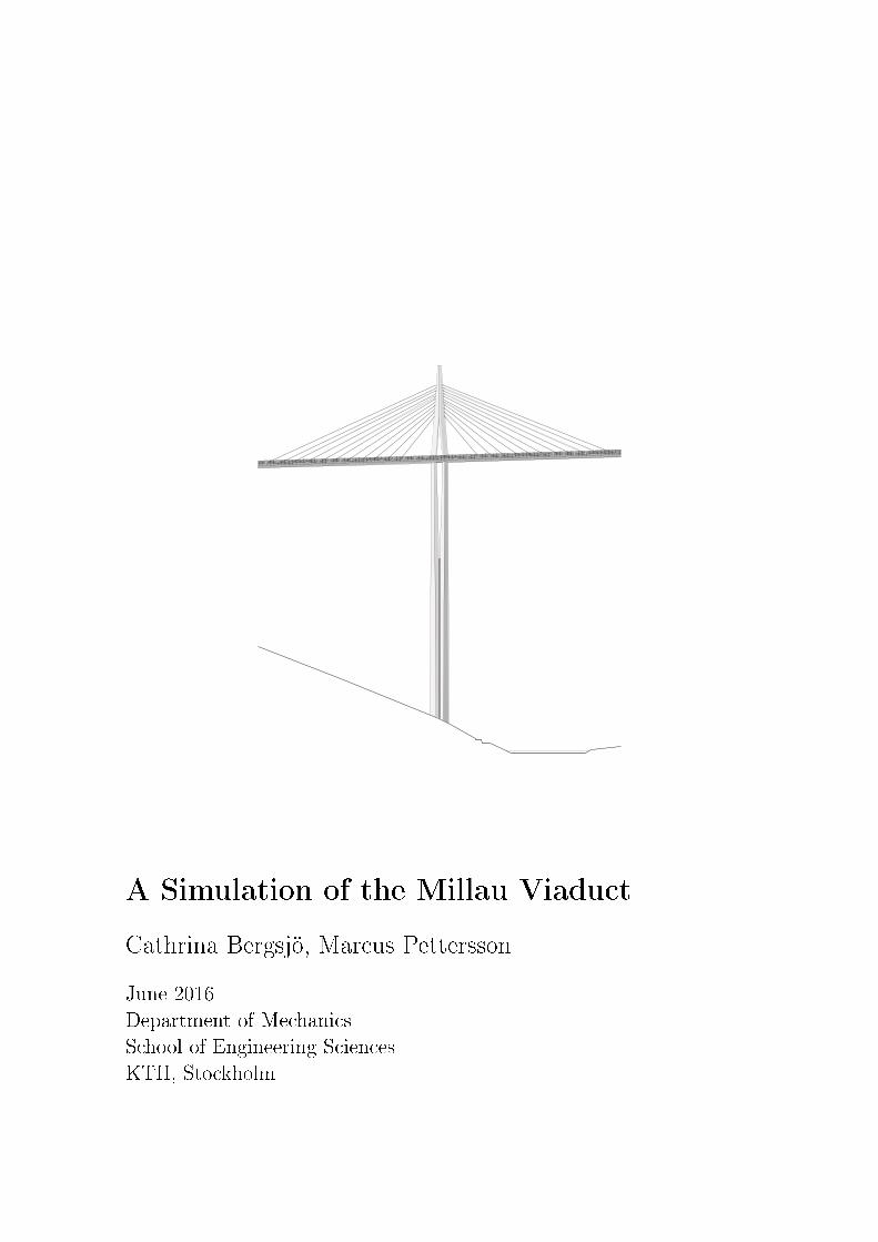
A Simulation of the Millau Viaduct
Cathrina Bergsjö, Marcus Pettersson
June 2016
Department of Mechanics
School of Engineering Sciences
KTH, Stockholm

c Cathrina Bergsjö, Marcus Pettersson 2016Royal Institute of Technology (KTH)School of Engineering SciencesDepartment of MechanicsStockholm, Sweden, 2016
Abstract
Cable-stayed bridges have become very popular over the last �ve decades due totheir aesthetic appeal, structural e�ciency, the limited amount of material usageand �nancial bene�ts. The rapid increase of new techniques creating longer spans,slender decks and more spectacular design has given rise to a major concern ofthe dynamic behavior of cable-stayed bridges. This has resulted in a more carefulmodelling procedure that will represent the reality in the most particular way. Amodel is simply an approximation of the reality, thus it is important to establishwhat simpli�cations and approximations that are reasonable to make in order forthe model to be as accurate as possible.
The Millau Viaduct is a cable-stayed bridge unique of its kind. At the time thatit was built it was breaking many records: span length, height of deck above thefoundations and the short construction time in just three years. Due to the slen-derness of the structure, the extreme height and the location in a deep valley, theviaduct is naturally subjected to external loads. This thesis attempts to describea performed dynamic nonlinear analysis of two models of the Millau Viaduct usingthe FEA packages SAP2000 and BRIGADE/Plus. The models have been re�nedin order to be compared between the programs and to the reality i.e. the measuredmode shapes and frequencies obtained from reports.
The viaduct required many speci�cally designed solutions in order to obtain theelegance and the aesthetic appeal. Approximations in geometry has been essentialdue to the many details that the viaduct consists of, but the details are nonethelessimportant to capture to get the structural mechanics correct. The support conditionshas been considered as important as these were designed to allow for movementthat were caused by a combination of the external loads and the slenderness of thestructure. The most critical support conditions were the deck-pier connection inwhich the piers are split into two columns equipped with spherical bearings allowingfor angular rotation. The two shafts were modelled by one single column and thespherical bearings were simulated by creating two alternative models; one assignedwith a pinned constraint to allow for the angular rotation and the second, since thissupport condition is in fact rigid has been assigned as �xed.
The SAP and BRIGADE models showed to be consistent with each other, thoughthe beam theories, Euler-Bernoulli were applied to the SAP model and Timoshenkoin BRIGADE. The alternative models with the di�erent constraints generated fairresults yet di�ers signi�cantly from each other. Alternative approaches towards themodelling have been addressed in the conclusions.
iii

Sammanfattning
Byggnationen av snedkabelbroar har ökat under de senaste fem decennierna på grundav sitt estetiska tilltalande, e�ektiva bärförmåga i proportion till mängden materialsom används och ekonomiska fördelar. Den snabba ökningen av nya tekniker har gettmöjlighet till längre spännvidder, smalare däck och mer spektakulär design. Dettahar gett upphov till en närmare studie av snedkabelbroars dynamiska respons ochökat kraven på en mer noggrann modellering för att ge en mer korrekt avbildning.En modell är enbart en approximation av verkligheten, därför är det viktigt attfastställa vilka förenklingar och approximationer som är rimliga för att modellenska bli en god och korrekt som möjligt.
Millaubron är en snedkabelbro, unik för sitt slag och rekordbrytande i många kat-egorier; spannlängden, höjden på tornen och byggtiden under endast tre år. Bronsslankhet, den extrema höjden och att den är belägen i en djup dal, medför ennaturlig påfrestning från yttre laster på bron. I denna masteruppsats beskrivs enutförd dynamisk icke-linjär analys av två modeller av Millaubron i FEA program-men SAP2000 och BRIGADE/Plus. Modellerna har för�nats stegvis för att kunnajämföras mellan programmen och mot uppmätta modformer och dess frekvenser somerhållits från rapporter.
För att Millaubron skulle få sitt speciella utseende krävdes många innovativa lös-ningar och detaljer. Approximationer i geometri har varit nödvändigt på grund avde många detaljer som bron består av, detaljer som är viktiga att fånga ur struk-turmekaniska aspekter. Det har lagts mycket vikt på upplagsvillkoren eftersom dessavar utformade för att möjliggöra rörelser som orsakades av en kombination av deyttre laster och strukturens slankhet. De mest kritiska upplagsvillkoren var mel-lan däcket och pelaren där pelaren är uppdelad i två mindre pelare utrustade medsfäriska lager som möjliggör vinkelrotation. De två mindre pelarna har modellerassom en pelare och de sfäriska upplagen simulerades genom att skapa två alternativamodeller - en tilldelad som fritt upplagd för att möjliggöra vinkelrotationen och detandra, eftersom dessa stöd anses styva, har modelleras som fast inspända.
SAP och BRIDAGE modellerna var konsekventa gentemot varandra, trots att balk-teorierna, Euler-Bernoulli användes i SAP och Timoshenko i BRIGADE. De alter-nativa modellerna genererade rättvisa resultat men skiljer sig från de uppmätta.Alternativa tillvägagångssätt för modelleringen har tagits upp i slutsatserna.
v

Preface
Many people have contributed on this journey completing this thesis, many whosehelp we could not have done this without. We hope that we have not forgottenanyone, but we realize that many more than the people mentioned below engagedin our thesis and we appreciate it so much.
The topic of this master thesis has been discussed with Michel Virlogeux, one ofthe designers of the Millau Viaduct, for two years before it was initiated. With thehelp from the faculty of Civil and Architectural Engineering at the Royal Instituteof Technology, it was established. Michel Virlogeux has been a key person for thismaster thesis to be completed and has been a great source of inspiration for theboth of us. We would like to thank Mr Virlogeux for his time and engagement in usand our thesis. We have had the privilege to experience and see the viaduct fromthe inside as well as from a far. This has been among the greatest experiences ofour lives and we cannot express our gratitude enough.
We would also like to say thank you to our professor and examiner Anders Erikssonat the division of the Mechanics, who has been a great support for many years andhas always encouraged us during the thesis. He has always been very helpful andnever too busy to discuss with us. We could not have asked for a more dedicatedexaminer and supervisor. He is a remarkable teacher worthy of great recognition.
Due to the lack of space at Mr Virlogeux's o�ce in Paris, we were o�ered space atTyréns AB which we would like to thank Mikael Hallgren for helping us with. Wewere able to complete this thesis with Mr Virlogeux as a supervisor on a distance.We would really like to direct our gratitude towards Tyréns AB, where we have beensupervised by Mahir Ülker-Kaustell and Fritz King. Their guidance and knowledgehave been valuable during the time we have spent at Tyréns. The sta� at Tyrénsdeserves a fair share of recognition as they have contributed with both knowledgeand good spirit.
In order to understand cable-stayed bridges and the importance of their behavior wehave been able to ask and discuss our conclusions and analyses with Mr Jean-YvesDel Forno at Greisch Bureau in Belgium. His pointers and knowledge has been veryvaluable, we are incredibly grateful to have gotten to learn from him. We wouldalso like to express our gratitude to Oystein Flakk at EDR Medeso whose adviceand courses within SAP2000 has been incredibly helpful.
The amount of material available on the internet of the Millau Viaduct is verylimited, we would like to thank Foster and Partners for allowing us to use one
vii

of their drawings on our front page and for sending us valuable and inspirationalmaterial with great hospitality. The sta� at Foster and Partners are a delightfulteam. Greisch Bureau has also been involved with contributing materials, drawingsand structural information that would come to be the foundation of this thesis.We are incredibly grateful for their help, for have been granted their con�denceand this opportunity. A huge thank you to Madam Marine Crouan, responsible forcommunication at Compagnie Ei�age, for arranging the incredible �eld visit to theviaduct and for making the Millau trip extraordinary.
Additional thanks to Bert Norlin for his help with the steel design calculations withgreat enthusiasm.
Last but not least, we would like to thank our families and friends for supportingus throughout the years at KTH, this report is dedicated to you.
Cathrina Bergsjö and Marcus Pettersson
viii
Contents
Abstract iii
Sammanfattning v
Preface vii
1 Introduction 1
1.1 Explanation of the Content . . . . . . . . . . . . . . . . . . . . . . . 1
1.2 The Viaduct of Millau . . . . . . . . . . . . . . . . . . . . . . . . . . 2
1.2.1 The Conceptual Design . . . . . . . . . . . . . . . . . . . . . . 3
1.2.2 The Box-Girder . . . . . . . . . . . . . . . . . . . . . . . . . . 3
1.2.3 The launching . . . . . . . . . . . . . . . . . . . . . . . . . . . 4
1.2.4 The Bridge Composition . . . . . . . . . . . . . . . . . . . . . 5
1.3 Introduction to the Programs . . . . . . . . . . . . . . . . . . . . . . 12
1.3.1 SAP2000 . . . . . . . . . . . . . . . . . . . . . . . . . . . . . . 12
1.3.2 BRIGADE/Plus . . . . . . . . . . . . . . . . . . . . . . . . . . 13
2 Background Study 15
2.1 Finite Element Analysis . . . . . . . . . . . . . . . . . . . . . . . . . 15
2.1.1 Advantages of FEA . . . . . . . . . . . . . . . . . . . . . . . . 15
2.2 Beam Theory . . . . . . . . . . . . . . . . . . . . . . . . . . . . . . . 16
2.3 Structural Dynamics . . . . . . . . . . . . . . . . . . . . . . . . . . . 17
2.3.1 Equation of Motion . . . . . . . . . . . . . . . . . . . . . . . . 17
2.3.2 Natural Frequencies and Mode Shapes . . . . . . . . . . . . . 19
2.3.3 Modal Analysis . . . . . . . . . . . . . . . . . . . . . . . . . . 19
ix
2.4 Introduction to Nonlinearity . . . . . . . . . . . . . . . . . . . . . . . 22
2.4.1 Nonlinearities Applied on Cable-stayed Bridges . . . . . . . . 23
2.4.2 The Cable Sag E�ect . . . . . . . . . . . . . . . . . . . . . . . 24
2.4.3 The Beam-column E�ect . . . . . . . . . . . . . . . . . . . . . 24
2.4.4 Large Displacements . . . . . . . . . . . . . . . . . . . . . . . 25
2.4.5 Newton-Raphson Method . . . . . . . . . . . . . . . . . . . . 26
2.5 The Cable . . . . . . . . . . . . . . . . . . . . . . . . . . . . . . . . . 27
2.6 OECS and MECS Method . . . . . . . . . . . . . . . . . . . . . . . . 31
2.6.1 OECS with an Equivalent Modulus of Elasticity . . . . . . . . 32
2.6.2 MECS with the Original Modulus of Elasticity . . . . . . . . . 34
3 Method 37
3.1 Prestudy . . . . . . . . . . . . . . . . . . . . . . . . . . . . . . . . . . 37
3.1.1 Literature Example . . . . . . . . . . . . . . . . . . . . . . . . 37
3.1.2 General Method . . . . . . . . . . . . . . . . . . . . . . . . . . 38
3.1.3 Results . . . . . . . . . . . . . . . . . . . . . . . . . . . . . . . 41
3.1.4 Discussion . . . . . . . . . . . . . . . . . . . . . . . . . . . . . 42
3.1.5 Conclusions . . . . . . . . . . . . . . . . . . . . . . . . . . . . 43
3.2 Modelling the Millau Viaduct . . . . . . . . . . . . . . . . . . . . . . 44
3.2.1 Bridge properties . . . . . . . . . . . . . . . . . . . . . . . . . 44
3.2.2 Material Properties . . . . . . . . . . . . . . . . . . . . . . . . 44
3.2.3 Geometrical Properties . . . . . . . . . . . . . . . . . . . . . . 45
3.2.4 Modelling Procedure . . . . . . . . . . . . . . . . . . . . . . . 51
3.3 The Analyzed Models . . . . . . . . . . . . . . . . . . . . . . . . . . 67
4 Results 69
4.1 Overview . . . . . . . . . . . . . . . . . . . . . . . . . . . . . . . . . . 69
4.1.1 Frequencies for a �xed connection . . . . . . . . . . . . . . . . 70
4.1.2 Frequencies for a pinned connection . . . . . . . . . . . . . . . 81
5 Concluding Remarks and Further Work 93
x

5.1 Discussion . . . . . . . . . . . . . . . . . . . . . . . . . . . . . . . . . 93
5.2 Conclusions . . . . . . . . . . . . . . . . . . . . . . . . . . . . . . . . 96
5.3 Alternative Approaches . . . . . . . . . . . . . . . . . . . . . . . . . . 97
Bibliography 99
A Calculations of Sectional Properties 103
A.1 The Theory of Cold-rolled Steel Pro�les . . . . . . . . . . . . . . . . 103
xi

Chapter 1
Introduction
1.1 Explanation of the Content
The thesis begins with an introduction to the topic under study, the design of theMillau Viaduct and the bridge composition in the �rst chapter. It is followed byan extensive background study on all essential factors that cable-stayed bridgesencounters, both in reality and in FEA. There among structural dynamics, thenonlinear e�ects, the modelling of signi�cant components i.e. cables and othernumerical solution methods. The background study was completed to obtain atheoretical background that would build the foundation of the method. It wascompleted to help strengthen the knowledge and prepare for the modelling so thatthe structural mechanics could be interpreted and simulated in the most accurateway.
The method consists of two parts; the pre-study that would help us get to know thesoftware that were utilized to complete the thesis and to understand the modelling ofcable-stayed bridges; and the modelling of the thesis topic, the Millau Viaduct, andhow the signi�cant factors in reality has been approximated in the two programs.
Discussion, conclusions and alternative approaches are provided based on the results.
1
CHAPTER 1. INTRODUCTION
1.2 The Viaduct of Millau
The small town Millau in southern France used to be one of the most famous bot-tlenecks in Europe. The town su�ered from bad reputation and massive congestionduring the summer holiday when the number travellers between Paris to Spainincreased. It could take more than 3-4 hours to get out of the tra�c jams. The SE-TRA, the design o�ce of the Highway Administration in France proposed a bridgethat would be linked to the A75 highway, to span the valley where the River Tarn�ows.
The greatest challenge for the completion of the A75 highway was to cross the riverTarn at such height and spanning the gap from one plateau to the other (Road-andtra�c). The �rst road alignments were proposed 1987 by CETE Mediterannee, butnone of the proposed were considered to be possible. The request was to locatethe bridge west of Millau, but due to the topography it was complicated. In 1989SETRA suggested a direct passing from the Causse Rouge in the north to the LarzacPlateau in the south by letting a high viaduct span the valley.
The head engineer Mr Michel Virlogeux presented a few suggestions to the concep-tual design that were evaluated by the team of SETRA. Pre-stressed box girders ofconstant depth built by the cantilever method, steel box-girders of constant depthincrementally launched either with a concrete slab or an orthotropic steel deck orsteel orthotropic box-girders of variable depth were a few alternatives that werediscussed. The ultimate choice fell on the orthotropic box-girder.
Once the conceptual design had been established, the new Highway Director ofSETRA was not convinced about the su�ciency of proposals on the designs madeby SETRA and decided to organize an international competition to develop otherconcepts. Eight design o�ces and seven architects were asked to contribute withtheir opinion on the designs made by SETRA and to propose new improvementsfrom both architectural and engineering perspective. Five projects were chosen toparticipate in the competition of designing the viaduct.
Though the competition was never a real competition, the assessment of the projectswere decided to be done by a jury of local politicians, architects and engineers. Thewinner, the architect sir Norman Foster, was announced the 1996. He had developedone of Michel Virlogeux's ideas of a cable-stayed bridge in either steel or concretewith multiple spans. At that time SETRA could no longer be responsible for thedesign, which was given to the winning team. Michel Virlogeux who had dedicatedmuch time to the project also had developed deep interest and decided to leaveSETRA to join Foster and his team. The three responsible design o�ces wereSogelerg, Europe Etudes Gecti and Serf, and the architect Norman Foster.
2
1.2. THE VIADUCT OF MILLAU
1.2.1 The Conceptual Design
The conceptual design was continued to be developed by Norman Foster and MichelVirlogeux. There were two main problems in the already created designs;
� To decide how to distribute the rigidity between the deck and pylons.
This could either be done by using a very rigid deck with a slender pylon, originallydeveloped by SETRA or a very rigid pylon made of either two columns connectedby the anchorage box, or by having a shape of an inverted V, which was assessedbeing able to suspend a �exible deck.
� To decide how �exible the end piers needed to be regarding to the horizontalforces.
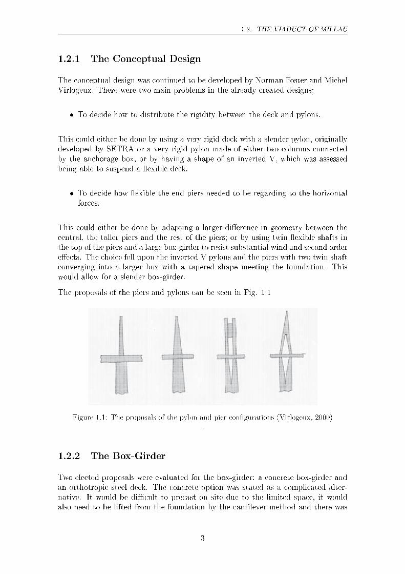
This could either be done by adapting a larger di�erence in geometry between thecentral, the taller piers and the rest of the piers; or by using twin �exible shafts inthe top of the piers and a large box-girder to resist substantial wind and second ordere�ects. The choice fell upon the inverted V pylons and the piers with two twin shaftconverging into a larger box with a tapered shape meeting the foundation. Thiswould allow for a slender box-girder.
The proposals of the piers and pylons can be seen in Fig. 1.1
Figure 1.1: The proposals of the pylon and pier con�gurations (Virlogeux, 2000)
.
1.2.2 The Box-Girder
Two elected proposals were evaluated for the box-girder: a concrete box-girder andan orthotropic steel deck. The concrete option was stated as a complicated alter-native. It would be di�cult to precast on site due to the limited space, it wouldalso need to be lifted from the foundation by the cantilever method and there was
3
CHAPTER 1. INTRODUCTION
no possibility to reach the deeper part of the valley due to the varying topography.There was not access to everywhere on the ground. The orthotropic steel deck wasevaluated as the best alternative, not only would it be much lighter, but it couldbe pushed by incremental launching from both ends. The steel pylons could also belaunched at the same time as the deck which proved to be most time e�cient.
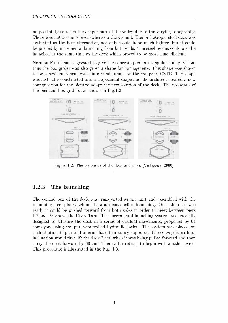
Norman Foster had suggested to give the concrete piers a triangular con�guration,thus the box-girder was also given a shape for homogeneity. This shape was shownto be a problem when tested in a wind tunnel by the company CSTB. The shapewas instead reconstructed into a trapezoidal shape and the architect created a newcon�guration for the piers to adapt the new solution of the deck. The proposals ofthe pier and box girders are shown in Fig.1.2
Figure 1.2: The proposals of the deck and piers (Virlogeux, 2000)
.
1.2.3 The launching
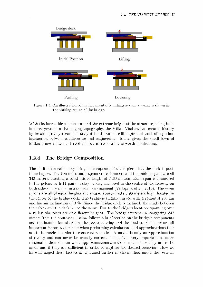
The central box of the deck was transported as one unit and assembled with theremaining steel plates behind the abutments before launching. Once the deck wasready it could be pushed forward from both sides in order to meet between piersP2 and P3 above the River Tarn. The incremental launching system was speciallydesigned to advance the deck in a series of gradual movements, propelled by 64conveyors using computer-controlled hydraulic jacks. The system was placed oneach abutments pier and intermediate temporary supports. The conveyors with aninclination would �rst lift the deck 2 cm, when it was being pulled forward and thencarry the deck forward by 60 cm. There after retract to begin with another cycle.This procedure is illustrated in the Fig. 1.3.
4
1.2. THE VIADUCT OF MILLAU
Initial Position Lifting
Pushing Lowering
Bridge deck
Figure 1.3: An illustration of the incremental launching system apparatus shown inthe visiting centre of the bridge.
With the incredible slenderness and the extreme height of the structure, being builtin three years in a challenging topography, the Millau Viaduct had created historyby breaking many records. Today it is still an incredible piece of work of a perfectinteraction between architecture and engineering. It has given the small town ofMillau a new image, enlarged the tourism and a name worth mentioning.
1.2.4 The Bridge Composition
The multi-span cable stay bridge is composed of seven piers that the deck is posi-tioned upon. The two most outer spans are 204 meters and the middle spans are all342 meters, creating a total bridge length of 2460 meters. Each span is connectedto the pylons with 11 pairs of stay-cables, anchored in the centre of the freeway onboth sides of the pylon in a semi-fan arrangement (Virlogeux et al., 2015). The sevenpylons are all of equal heights and shape, approximately 90 meters high, located inthe center of the bridge deck. The bridge is slightly curved with a radius of 200 kmand has an inclination of 3 %. Since the bridge deck is inclined, the angle betweenthe cables and the deck is not the same. Due to the bridge's location, spanning overa valley, the piers are of di�erent heights. The bridge stretches a staggering 342meters from the abutment. Below follows a brief section on the bridge's componentsand the installation of cables, the pre-tensioning and the �nal stage. These are allimportant factors to consider when performing calculations and approximations thatare to be made in order to construct a model. A model is only an approximationof reality and can never be exactly correct. Thus, it is very important to makereasonable decisions on what approximations are to be made, how they are to bemade and if they are su�cient in order to capture the desired behavior. How wehave managed these factors is explained further in the method under the sections
5
CHAPTER 1. INTRODUCTION
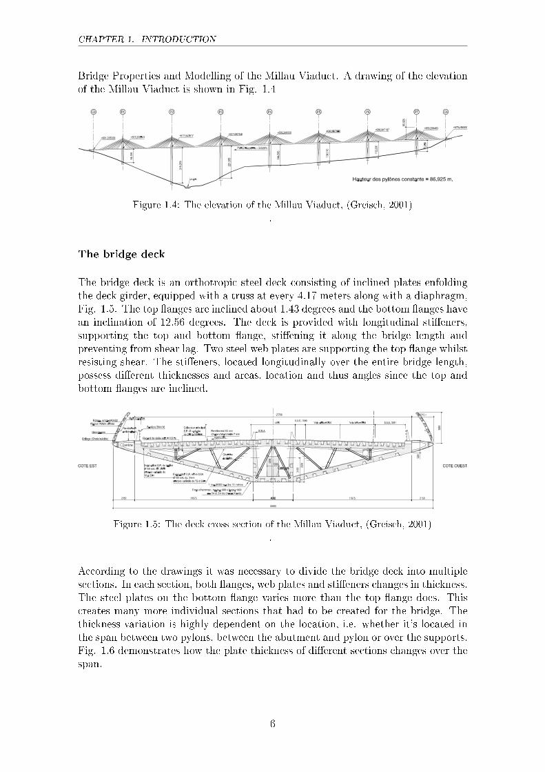
Bridge Properties and Modelling of the Millau Viaduct. A drawing of the elevationof the Millau Viaduct is shown in Fig. 1.4
Figure 1.4: The elevation of the Millau Viaduct, (Greisch, 2001)
.
The bridge deck
The bridge deck is an orthotropic steel deck consisting of inclined plates enfoldingthe deck girder, equipped with a truss at every 4.17 meters along with a diaphragm,Fig. 1.5. The top �anges are inclined about 1.43 degrees and the bottom �anges havean inclination of 12.56 degrees. The deck is provided with longitudinal sti�eners,supporting the top and bottom �ange, sti�ening it along the bridge length andpreventing from shear lag. Two steel web plates are supporting the top �ange whilstresisting shear. The sti�eners, located longitudinally over the entire bridge length,possess di�erent thicknesses and areas, location and thus angles since the top andbottom �anges are inclined.
Figure 1.5: The deck cross section of the Millau Viaduct, (Greisch, 2001)
.
According to the drawings it was necessary to divide the bridge deck into multiplesections. In each section, both �anges, web plates and sti�eners changes in thickness.The steel plates on the bottom �ange varies more than the top �ange does. Thiscreates many more individual sections that had to be created for the bridge. Thethickness variation is highly dependent on the location, i.e. whether it's located inthe span between two pylons, between the abutment and pylon or over the supports.Fig. 1.6 demonstrates how the plate thickness of di�erent sections changes over thespan.
6
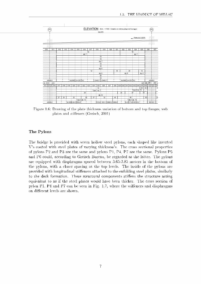
1.2. THE VIADUCT OF MILLAU
Figure 1.6: Drawing of the plate thickness variation of bottom and top �anges, webplates and sti�eners (Greisch, 2001)
.
The Pylons
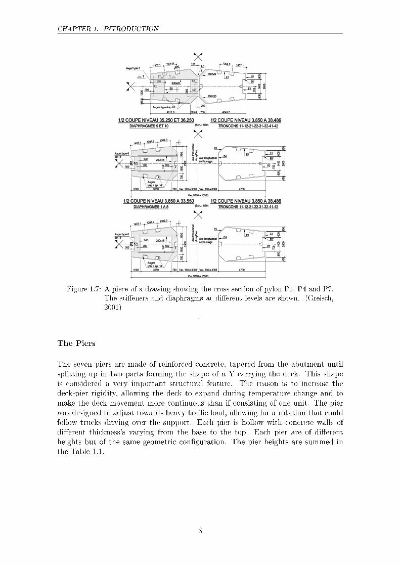
The bridge is provided with seven hollow steel pylons, each shaped like invertedV's coated with steel plates of varying thickness's. The cross sectional propertiesof pylons P2 and P3 are the same and pylons P1, P4, P7 are the same. Pylons P5and P6 could, according to Greisch Bureau, be regarded as the latter. The pylonsare equipped with diaphragms spaced between 3.65-3.85 meters in the bottom ofthe pylons, with a closer spacing at the top levels. The inside of the pylons areprovided with longitudinal sti�eners attached to the enfolding steel plates, similarlyto the deck formation. These structural components sti�ens the structure actingequivalent to as if the steel plates would have been thicker. The cross section ofpylon P1, P4 and P7 can be seen in Fig. 1.7, where the sti�eners and diaphragmson di�erent levels are shown.
7
CHAPTER 1. INTRODUCTION
Figure 1.7: A piece of a drawing showing the cross section of pylon P1, P4 and P7.The sti�eners and diaphragms at di�erent levels are shown. (Greisch,2001)
.
The Piers
The seven piers are made of reinforced concrete, tapered from the abutment untilsplitting up in two parts forming the shape of a Y carrying the deck. This shapeis considered a very important structural feature. The reason is to increase thedeck-pier rigidity, allowing the deck to expand during temperature change and tomake the deck movement more continuous than if consisting of one unit. The pierwas designed to adjust towards heavy tra�c load, allowing for a rotation that couldfollow trucks driving over the support. Each pier is hollow with concrete walls ofdi�erent thickness's varying from the base to the top. Each pier are of di�erentheights but of the same geometric con�guration. The pier heights are summed inthe Table 1.1.
8
1.2. THE VIADUCT OF MILLAU
Table 1.1: Heights of the piers
Pier Height(m)
P1 94.50P2 244.96P3 221.05P4 144.21P5 136.42P6 111.94P7 77.56
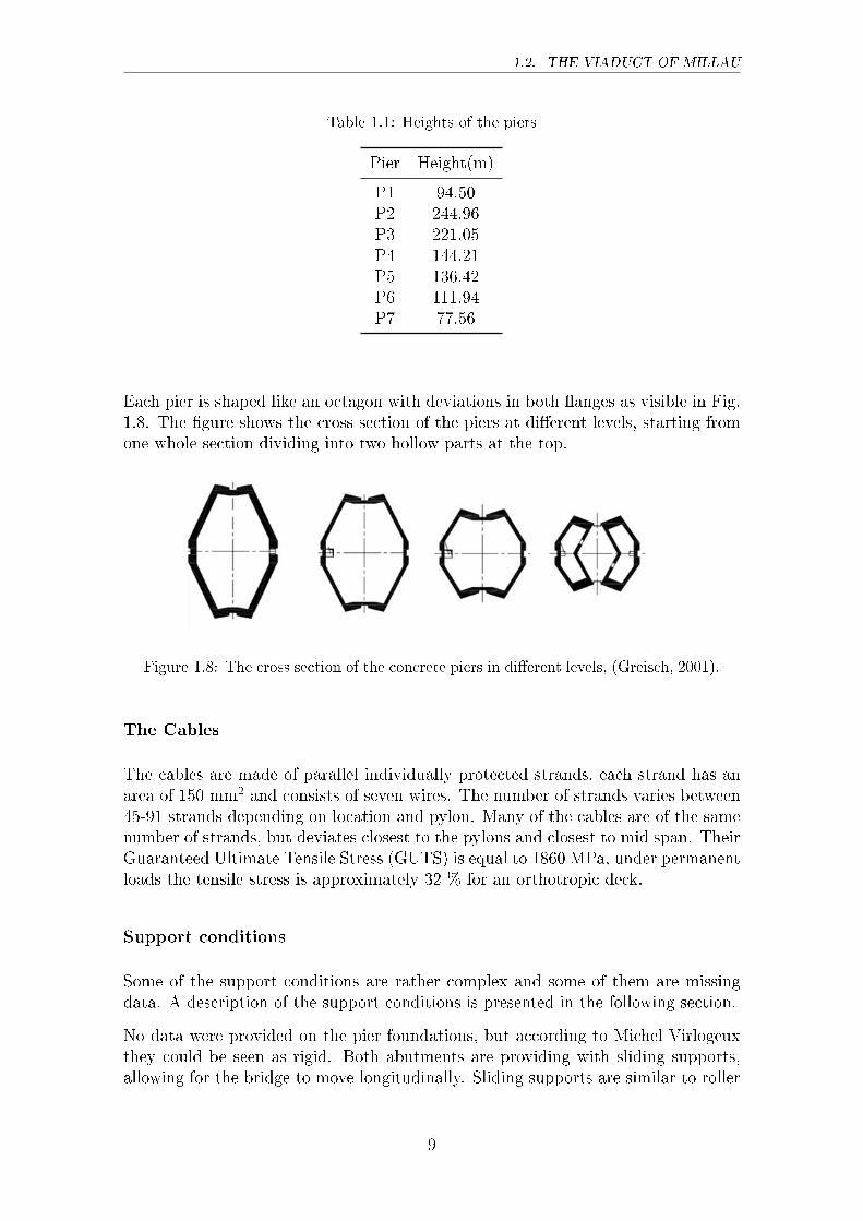
Each pier is shaped like an octagon with deviations in both �anges as visible in Fig.1.8. The �gure shows the cross section of the piers at di�erent levels, starting fromone whole section dividing into two hollow parts at the top.
Figure 1.8: The cross section of the concrete piers in di�erent levels, (Greisch, 2001).
The Cables
The cables are made of parallel individually protected strands, each strand has anarea of 150 mm2 and consists of seven wires. The number of strands varies between45-91 strands depending on location and pylon. Many of the cables are of the samenumber of strands, but deviates closest to the pylons and closest to mid span. TheirGuaranteed Ultimate Tensile Stress (GUTS) is equal to 1860 MPa, under permanentloads the tensile stress is approximately 32 % for an orthotropic deck.
Support conditions
Some of the support conditions are rather complex and some of them are missingdata. A description of the support conditions is presented in the following section.
No data were provided on the pier foundations, but according to Michel Virlogeuxthey could be seen as rigid. Both abutments are providing with sliding supports,allowing for the bridge to move longitudinally. Sliding supports are similar to roller
9
CHAPTER 1. INTRODUCTION
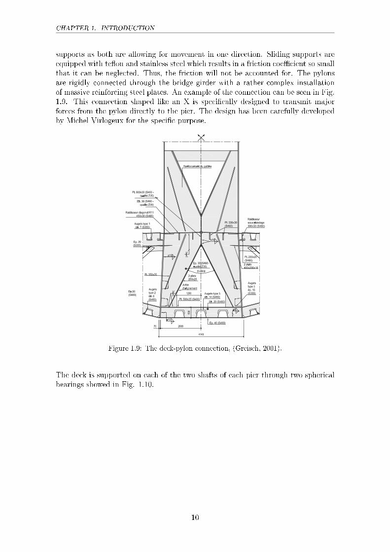
supports as both are allowing for movement in one direction. Sliding supports areequipped with te�on and stainless steel which results in a friction coe�cient so smallthat it can be neglected. Thus, the friction will not be accounted for. The pylonsare rigidly connected through the bridge girder with a rather complex installationof massive reinforcing steel plates. An example of the connection can be seen in Fig.1.9. This connection shaped like an X is speci�cally designed to transmit majorforces from the pylon directly to the pier. The design has been carefully developedby Michel Virlogeux for the speci�c purpose.
Figure 1.9: The deck-pylon connection, (Greisch, 2001).
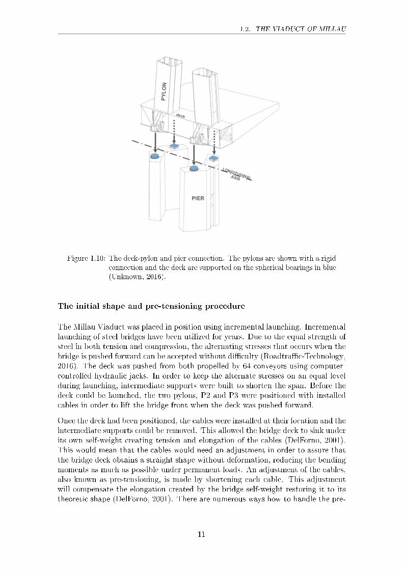
The deck is supported on each of the two shafts of each pier through two sphericalbearings showed in Fig. 1.10.
10
1.2. THE VIADUCT OF MILLAU
Figure 1.10: The deck-pylon and pier connection. The pylons are shown with a rigidconnection and the deck are supported on the spherical bearings in blue(Unknown, 2016).
The initial shape and pre-tensioning procedure
The Millau Viaduct was placed in position using incremental launching. Incrementallaunching of steel bridges have been utilized for years. Due to the equal strength ofsteel in both tension and compression, the alternating stresses that occurs when thebridge is pushed forward can be accepted without di�culty (Roadtra�c-Technology,2016). The deck was pushed from both propelled by 64 conveyors using computer-controlled hydraulic jacks. In order to keep the alternate stresses on an equal levelduring launching, intermediate supports were built to shorten the span. Before thedeck could be launched, the two pylons, P2 and P3 were positioned with installedcables in order to lift the bridge front when the deck was pushed forward.
Once the deck had been positioned, the cables were installed at their location and theintermediate supports could be removed. This allowed the bridge deck to sink underits own self-weight creating tension and elongation of the cables (DelForno, 2001).This would mean that the cables would need an adjustment in order to assure thatthe bridge deck obtains a straight shape without deformation, reducing the bendingmoments as much as possible under permanent loads. An adjustment of the cables,also known as pre-tensioning, is made by shortening each cable. This adjustmentwill compensate the elongation created by the bridge self-weight restoring it to itstheoretic shape (DelForno, 2001). There are numerous ways how to handle the pre-
11
CHAPTER 1. INTRODUCTION
tensioning of the cable and the initial shape of the bridge. How this is managed inthe models are explained further in the section Modelling of the Millau Viaduct.
1.3 Introduction to the Programs
1.3.1 SAP2000
The SAP name has been active in engineering analytical methods for over 30 yearsago developed by CSI America. SAP2000 is a general-purpose civil engineeringsoftware suitable for the analysis and design of any type of structural system (CSI,2016). SAP2000 is thus adapted for any structure, however, there is a softwarespeci�cally for bridge structure, CSIBridge, which aims to pick up factors onlytreated in bridge analysis.
SAP2000 handles basic as well as advanced systems in both 2D and 3D, with ei-ther simple or complex geometry in both straight and nonlinear analysis. SAP2000provides the user with the classic FE elements; frame, shell and solid elements, thepossibility of modelling linear or curved members, cables, using a speci�c nonlinearelement which accounts for the sag e�ect nonlinearity, and post-tensioned tendons.There are link elements to model springs, dampers isolators and the associated non-linear behavior.
When conventional beam or frame cross section is desired SAP2000 has a built inextensive library with both material and geometric properties from di�erent stan-dards and codes from across the globe. If the user wishes a speci�c cross sectionwhich is not available, the user may specify the geometry using a Section Designer.When a model is created a built in template, the SAPFire Analysis Engine, auto-matically converts the assembly into a FE-model by meshing the material domainwith a network of quadrilateral sub-elements. The user may, of course, determinethe mesh which is found most appropriate for the analysis. SAP2000 is adapted tomodel structural systems of any kind and complexity.
For the analysis procedure, the user is free to complement the standard analysisby performing in dynamic and nonlinear analysis. The dynamic analysis includeseigen analysis and Ritz analysis. Geometric nonlinearity is considered by P-� ef-fects, which is included during nonlinear buckling accompanied by large displace-ment e�ects. The nonlinear analysis includes material nonlinearity which capturesinelastic and limit-state behavior as well as time-dependent creep and shrinkagebehavior. Dynamic methods include the response-spectrum, steady-state and time-history analysis.
For the interested user we refer to CSI America's website in which all of the featuresthat SAP2000 provides are described in more detail.
12
1.3. INTRODUCTION TO THE PROGRAMS
1.3.2 BRIGADE/Plus
BRIGADE/Plus is a �nite element program, providing a powerful and completerange of analysis procedures in an interactive and visual environment. It is de-signed to implement advanced analysis and design of all types of bridges and civilstructures (Scanscot, 2016). BRIGADE/Plus provides a wide range of function-alities, including prede�ned loads, load combinations and moving vehicle loads inaccordance to design codes like the Eurocodes. The program provides an extensiverange of analysis procedures such as: linear and nonlinear static response, naturalfrequency extraction and steady-state dynamic response.
For the nonlinearities BRIGADE/Plus has the capability to handle geometrical non-linearities, the behavior of nonlinear material and also nonlinear contact interactions.
BRIGADE/Plus, is based on the FE-software ABAQUS and consist of three parts:
� A solver based on ABAQUS
� GUI (Graphical User Interface) based on ABAQUS/CAE
� Technology developed at Scanscot Technology
Since BRIGADE/Plus is focusing on bridges and civil structures, some of the fea-tures in ABAQUS have not been included, but the procedure of modelling is thesame. Each module is well de�ned for what to do in each step along the path ofmodelling the structure.
Each part's geometry is parametric and feature based, allowing for modelling ofcomplex geometries. The properties of the model and its attributes are easily as-signed to the selected part, like material and section properties to the de�ned region.Each part is created separately and then assembled together with assigned bound-ary conditions, interactions between the parts and loads acting on the structure tocreate a model to be analyzed.
Di�erent types of load combinations and the distribution of the loads can be ap-plied to the model. The loads can either be concentrated, distributed, a pressureload or a body force, but also it could be a combination of them. When meshing,BRIGADE/Plus contains a function to perform an automatic mesh of a region, butthe mesh can also be done manually be applying seeds globally or locally. The vari-ation of element families that can be utilized in BRIGADE/Plus is extensive witha few examples provided below.
� Truss elements
� Beam elements
� Shell elements
� Solid elements
13

CHAPTER 1. INTRODUCTION
The calculated results are then visualized in 3D plots and 2D graphs.
14
Chapter 2
Background Study
2.1 Finite Element Analysis
Finite element method (FEM) also referred to as �nite element analysis (FEA) isa numerical solution method that provides an approximate solution for boundaryvalue problems. The method is applied in engineering as a computational toolfor performing analysis, described mathematically as a di�erential equation or anintegral expression. FEM subdivides the domain into smaller and simpler elementscalled �nite elements. To form the complete structure these elements are assembledby connecting points at the end of each element, called nodes. The elements arearranged as a mesh structure and represented by systems of equation to be solvedat the nodes. It can either be a linear or a non-linear system. FEA is a good toolwhen analyzing a complicated area, an area with non-consistent shape or when thelevel of details varies over the domain. (Cook et al., 2002)
2.1.1 Advantages of FEA
The very �rst thing to do when performing a FEA is to identify the problem. Whenthe problem is identi�ed, the user should be able to answer the following questions:how much and what kind of information must be gathered to perform the analysis,what kind of modelling techniques should be used and what kind of solutions andresults are important and expected.
Some advantages for using FEA is listed below. (Cook et al., 2002)
� FEA is applicable to any �eld problems described with a partial di�erentialequation: heat transfer, stress analysis etc.
� Boundary conditions and loadings are not restricted.
� The properties of the material may di�er from one element to another.
15
CHAPTER 2. BACKGROUND STUDY
� The di�erent elements may have di�erent behaviors from their di�erent math-ematical expressions.
� The subdivision of the domain gives an accurate representation of a complexgeometry so there are no geometric restrictions.
� By improving the mesh with more elements the representation of the totalsolution is easily captured and also the local e�ects.
2.2 Beam Theory
There are several beam theories based on various assumptions, but the most com-monly used in structural mechanics are the Euler-Bernoulli and the Timoshenkobeam theories. Both of these theories are utilized in this thesis and a short descrip-tion of them is presented below.
A beam is de�ned as a 3D structure with one of its dimensions much larger than theother two. The axis of the beam is de�ned along its longer dimension, with a cross-section that varies smoothly along the beam (Bauchau and Craig, 2009). The beamtheory is based on this de�nition, and provides a one dimensional approximation ofa three dimensional continuum (SIMULIA, 2011). The beam theory also referredto as the solid mechanics theory of beams, provides a simple way to analyze a widerange of structures and is a very important tool for structural analysis (Bauchau andCraig, 2009). Because the theory is easy to apply and the computational time in FE-programs becomes short it is useful in a pre-design phase. Depending on the analysis,the demands for details vary, and a beam model is therefore a great supplement fora shell model depending on the analysis. This is why beam elements are oftenpreferred, because of their simple geometry and their few degrees of freedom.
The Euler-Bernoulli beam theory is simple and very useful but it has its limitations,since it is known as shear in-deformable. Elements that are assigned to this theorywill work under three kinematic assumptions, called the Euler-Bernoulli assumptions(Bauchau and Craig, 2009)
� The cross-section is in�nitely rigid in its own plane.
� The cross-section of the beam remains plane after deformation.
� The cross-section remains normal to the deformed axis of the beam.
These assumptions are acceptable when analyzing long, slender isotropic beamswhere the cross-sectional dimensions are small compared to distances along its axis(Bauchau and Craig, 2009). These distances are typically the distances betweensupports, distances between gross changes in cross-sections or the wavelength of thehighest mode existing in the dynamic response. In order to neglect shear �exibility,and therefore be able to apply the Euler-Bernoulli beam theory, it is said that the
16
2.3. STRUCTURAL DYNAMICS
slenderness ratio should be less than 1/15. Were the slenderness ratio is the ratiobetween cross-sectional dimensions and axial distance (SIMULIA, 2011).
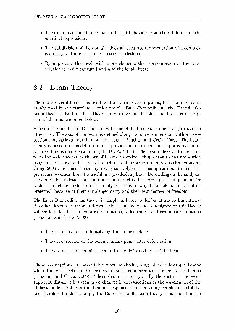
When the thickness of the beams becomes larger, the shear deformations cannot beneglected and this will con�ict with the Euler-Bernoulli assumptions. The Timo-shenko beam theory includes both the e�ect of shear deformation and the e�ect ofrotational inertia, when analyzing the vibrations of a beam (Bauchau and Craig,2009), but represents bending less well. Timoshenko beams can also be used forboth thick and slender beams. The theory is legit as long as the slenderness ratio isless than 1/8. When the cross-section becomes greater in comparison to the axiallength, the behavior of the structure can no longer be described accurately enoughas a function of axial position, and another element type has to be taken into con-sideration (SIMULIA, 2011). Fig. 2.1 shows the di�erent deformation of beamsusing the two theories. It can be seen that the cross-section of the Euler-Bernoullibeam remains normal to the axis during bending, whilst the Timoshenko beam de-forms. In a �nite element form, the Timoshenko beam on the other hand representscurvature much less accurately.
w
Q
TimoshenkoEuler-Bernoulli
M
Z
X
h
h
Figure 2.1: The Timoshenko beam experience shear deformation when under bend-ing while the Euler-Bernoulli beam does not. Re-drawn from Wikipedia(2016).
2.3 Structural Dynamics
2.3.1 Equation of Motion
The equation of motion is used to �nd the displacement or the deformation ofan idealized structure that is assumed to be linearly elastic and subjected to andexternal force p over a time period, t. The equation is derived from Newtons secondlaw of motion and can for a single degree of freedom be seen as:
m�u+ c _u+ ku = p (t) (2.1)
17
CHAPTER 2. BACKGROUND STUDY
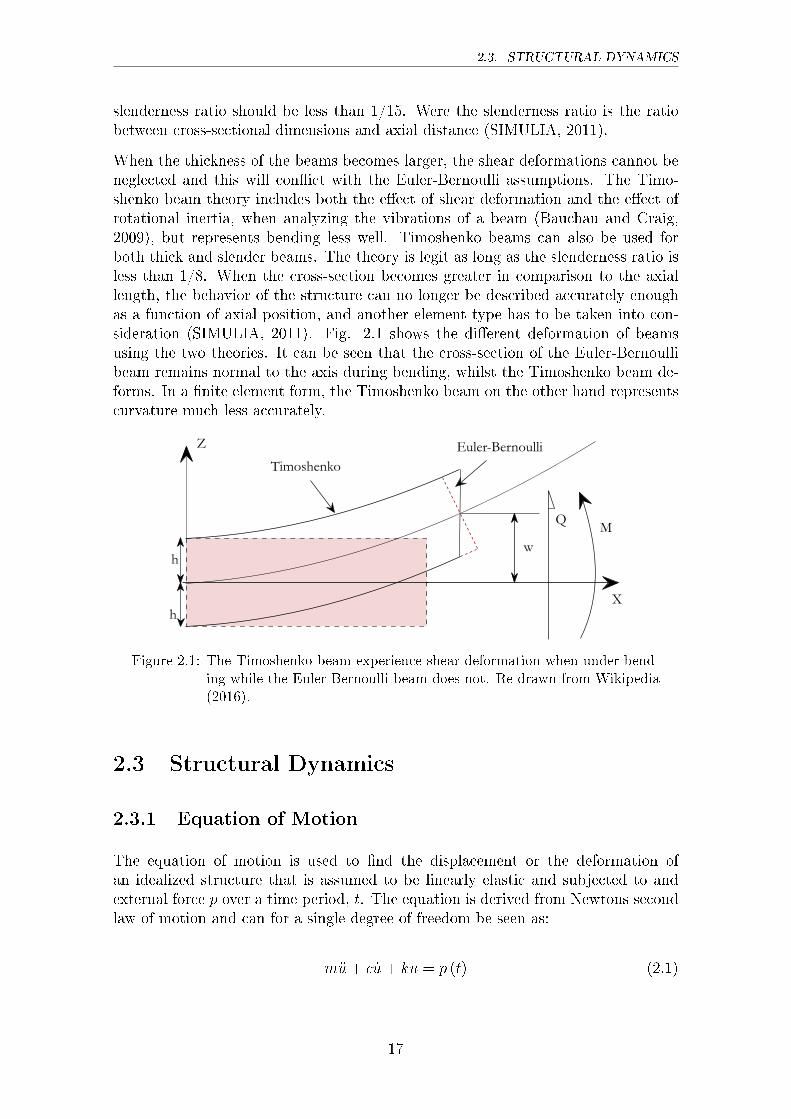
Fig. 2.2 visualizes how the equation of motion describes an idealized one-story struc-ture, subjected to an external force p(t). As the equation shows, the whole structureis dependent on three separate components, each component will be described in thischapter.
Mass p(t)
viscousdamper
fs
Displacement uVelocity u'acceleration u''
Displacement u
= +...
..+
ft
Acceleration u''
fD
velocity u'
+
a) b)
c) d)
Figure 2.2: Components of the system. Re-drawn from Chopra (2012).(a) Whole system; (b) Sti�ness; (c) Damping; (d) Mass
� b: Only the sti�ness component
� c: Only the damping component
� d: only the mass component
For a linear system the lateral force fS is written as lateral sti�ness times the de-formation, when disregarding damping and mass component:
fS = ku (2.2)
Damping is expressed as 'the process by which vibration steadily diminishes in am-plitude' (Chopra, 2012), and could therefore depend on various factors, e.g. frictionof steel connectors and opening and closing of microcracks in concrete. Therefore thedamping is idealized. In the commonly assumed linear viscous damper the damperforce fD is calculated as the damper velocity times the viscous damping coe�cient:
fD = c _u (2.3)
Newton's second law of motion explains the behavior of an object where the existingforces might be unbalanced, according to:
p(t) = m�u (2.4)
18
2.3. STRUCTURAL DYNAMICS
p(t) is the sum of all acting external forces. In the studied case this leads to:
fe � fS � fD = m�u (2.5)
Where fe represents the driving force on the system. When substituting the internalforces with the equations just presented we receive:
m�u+ c _u+ ku = fe (2.6)
2.3.2 Natural Frequencies and Mode Shapes
Many scenarios can cause a structure to move, sway and vibrate. Movements ofsuch can be induced by earthquakes, the pistons of an engine and moving tra�cloads for example. Mode shapes are the basic deformation patterns in which theundamped structurure can vibrate without external driving force. These movementsare quanti�able by measuring them in meters and the acceleration in the directionwhich it moves or by how rapid the vibration is occurring.
A structure is said to be experiencing free vibration when disturbed from the staticequilibrium and allowed to continue to vibrate freely without external sources ex-citing the structure (Bauchau and Craig, 2009). The term free vibration means thestate in which the structural system is allowed to oscillate in in�nity, and since allstructures are equipped with some sort of damping, either external or internal, freevibration only exists in theory.
Natural frequency is explained as the system's frequency at which it tends to oscil-late in the absence of any driving or damping force. There have been many damageswhere dynamics has played a vital role, there among the example of the TacomaNarrows Bridge in Washington State. If the system is excited such that the input fre-quency from external sources coincides with one of the system's natural frequencies,the system will undergo resonance (Hall, 2016). Resonance is typically somethingthat must be avoided. Once the system is experiencing resonance large amplitudeswill follow and thus analysing the dynamic behavior is crucial for all structures. Thishas become more relevant today due to all new techniques and extreme structureskeeps being developed e.g. more slender bridges, tracks for high speed trains, skyrising buildings both in and out of seismic zones. However, problems with too largeamplitudes can be recti�ed by sti�ening the structure or its components in the rightplaces to shift the natural frequencies away from the input frequencies (Hall, 2016).
2.3.3 Modal Analysis
Modal analysis also known as the mode superposition method is a linear dynamic-response procedure which computes and superimposes vibration mode shapes todescribe a structure's deformation pattern.
19
CHAPTER 2. BACKGROUND STUDY
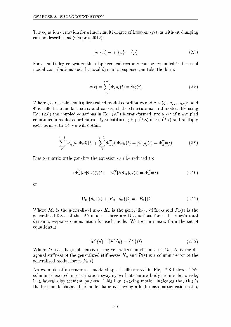
The equation of motion for a linear multi degree of freedom system without dampingcan be describes as (Chopra, 2012):
[m]f�ug+ [k]fug = fpg (2.7)
For a multi degree system the displacement vector u can be expanded in terms ofmodal contributions and the total dynamic response can take the form.
u(t) =r=1XN
�rqr(t) = �q(t) (2.8)
Where qr are scalar multipliers called modal coordinates and q is (q1, q2, ...qN)T and� is called the modal matrix and consist of the structure natural modes. By usingEq. (2.8) the coupled equations in Eq. (2.7) is transformed into a set of uncoupledequations in modal coordinates. By substituting Eq. (2.8) in Eq.(2.7) and multiplyeach term with �T
n we will obtain:
r=1XN
�Tn [m]�r �qr(t) +
r=1XN
�Tn [k]�rqr(t) = [�][q](t) = �T
np(t) (2.9)
Due to matrix orthogonality the equation can be reduced to:
(�Tn [m]�n)�qn(t) + (�T
n [k]�n)qn(t) = �Tnp(t) (2.10)
or
[Mn]f�qng(t) + [Kn]fqng(t) = fPng(t) (2.11)
Where Mn is the generalized mass Kn is the generalized sti�ness and Pn(t) is thegeneralized force of the nth mode. There are N equations for a structure's totaldynamic response one equation for each mode. Written in matrix form the set ofequations is:
[M ]f�qg+ [K]fqg = fPg(t) (2.12)
Where M is a diagonal matrix of the generalized modal masses Mn, K is the di-agonal sti�ness of the generalized sti�nesses Kn and P (t) is a column vector of thegeneralized modal forces Pn(t)
An example of a structure's mode shapes is illustrated in Fig. 2.3 below. Thiscolumn is excited into a motion swaying with its entire body from side to side,in a lateral displacement pattern. This �rst swaying motion indicates that this isthe �rst mode shape. The mode shape is showing a high mass participation ratio,
20
2.3. STRUCTURAL DYNAMICS
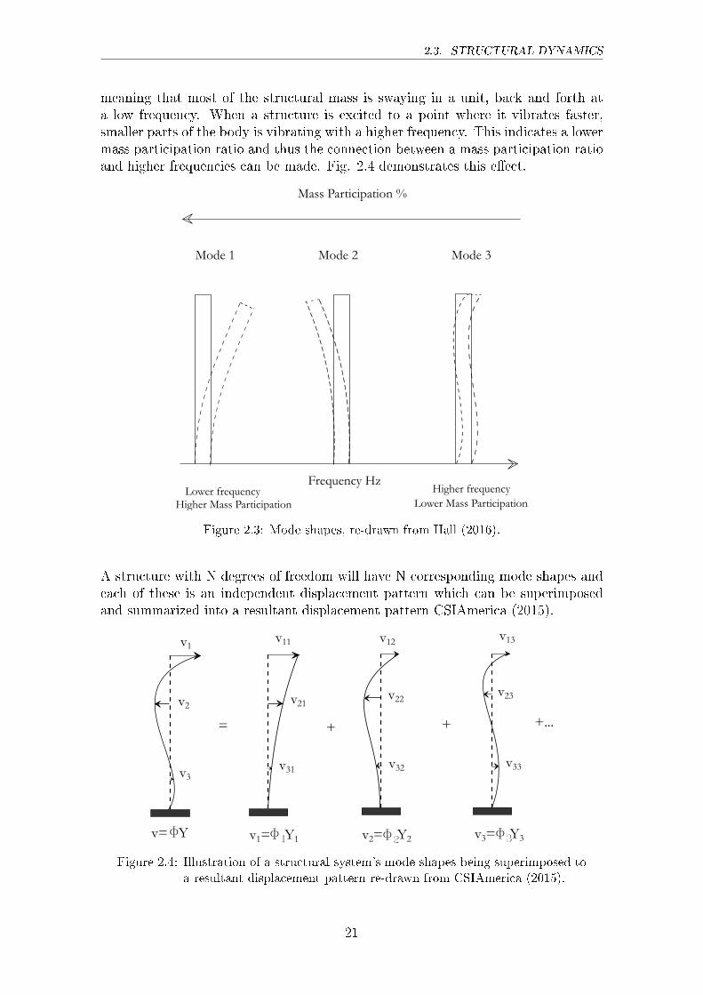
meaning that most of the structural mass is swaying in a unit, back and forth ata low frequency. When a structure is excited to a point where it vibrates faster,smaller parts of the body is vibrating with a higher frequency. This indicates a lowermass participation ratio and thus the connection between a mass participation ratioand higher frequencies can be made. Fig. 2.4 demonstrates this e�ect.
Frequency Hz
Mass Participation %
Mode 1 Mode 2 Mode 3
Lower frequencyHigher Mass Participation
Higher frequencyLower Mass Participation
Figure 2.3: Mode shapes, re-drawn from Hall (2016).
A structure with N degrees of freedom will have N corresponding mode shapes andeach of these is an independent displacement pattern which can be superimposedand summarized into a resultant displacement pattern CSIAmerica (2015).
v1
v2
v3
= + + +...
v11
v22v21v23
v31 v32 v33
v13v12
v= Y v1= Y1 v2= Y2 v3= Y3F F1 F2 F3
Figure 2.4: Illustration of a structural system's mode shapes being superimposed toa resultant displacement pattern re-drawn from CSIAmerica (2015).
21
CHAPTER 2. BACKGROUND STUDY
2.4 Introduction to Nonlinearity
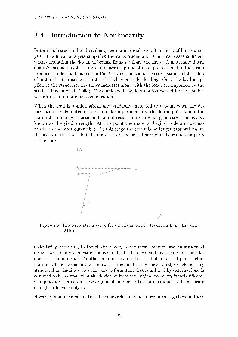
In terms of structural and civil engineering materials we often speak of linear anal-ysis. The linear analysis simpli�es the calculations and is in most cases su�cientwhen calculating the design of beams, frames, pillars and more. A materially linearanalysis means that the stress of a materials properties are proportional to the strainproduced under load, as seen in Fig.2.5 which presents the stress-strain relationshipof material. It describes a material's behavior under loading. Once the load is ap-plied to the structure, the stress increases along with the load, accompanied by thestrain (Heyden et al., 2008). Once unloaded the deformation caused by the loadingwill return to its original con�guration.
When the load is applied afresh and gradually increased to a point when the de-formation is substantial enough to deform permanently, this is the point where thematerial is no longer elastic and cannot return to its original geometry. This is alsoknown as the yield strength. At this point the material begins to deform perma-nently, in the most outer �bre. At this stage the strain is no longer proportional tothe stress in this area, but the material still behaves linearly in the remaining partsin the core.
Es
f
fufy
e
Figure 2.5: The stress-strain curve for ductile material. Re-drawn from Autodesk(2016).
Calculating according to the elastic theory is the most common way in structuraldesign, we assume geometric changes under load to be small and we do not considercracks in the material. Another common assumption is that no out of plane defor-mation will be taken into account. In a geometrically linear analysis, elementarystructural mechanics states that any deformation that is induced by external load isassumed to be so small that the deviation from the original geometry is insigni�cant.Computations based on these arguments and conditions are assumed to be accurateenough in linear analysis.
However, nonlinear calculations becomes relevant when it requires to go beyond these
22
2.4. INTRODUCTION TO NONLINEARITY
boarders. Nonlinearity in structural and civil engineering structures is present inthe following ways: geometrical, boundary and material nonlinearities (Sönnerlind,2016). Geometrical nonlinearity occurs in models with large deformation or rotation.Material nonlinearity, as discussed above, appears when the material is subjected toexternal load which causes higher stress than the material yield stress. Boundarylinearities occur when external loads change a structure's boundary conditions. Inproblems like these there are no linear relationship between the external load andthe resulting contact area.
For a linear structure, in a �nite element simulation, the relationship between theapplied loads and the displacements is described by:
�K� fdg = ffg (2.13)
where K is the sti�ness matrix which describes the structural degrees of freedom forthe structure (Fleming, 1979). In linear analysis, this sti�ness matrix is constantduring loading. Meanwhile most engineering problems consist of nonlinear e�ects,linear analyses has proven to be accurate enough in many cases, but there are excep-tions when nonlinear e�ects cannot be ignored. For nonlinear structures equilibriumequations cannot be described with a simple algebraic expression as we do in linearproblems.
Today, there are many �nite element programs that provide static as well as dynamicanalysis, linear and nonlinear analysis which has a created tremendous possibilitiesand progress to handle complex structures. For instance, when obtaining a solutionfor the correct cable forces, the solution process is most often iterative. An iterativesolution procedure is utilized in this master thesis for the �nal result.
2.4.1 Nonlinearities Applied on Cable-stayed Bridges
We have noted the increase in popularity constructing cable-stayed bridges. Thedesign of them has become more complex and extravagant. As the spans increaseso do the concerns about safety of these structures, which increases the demandson the analysis (Freire et al., 2006). The consideration for geometrical and materialnonlinear e�ects cannot be ignored, in fact they must be carefully evaluated. �Oneof the main di�culties which an engineer encounters when faced with the problem ofdesigning a cable-stayed bridge is the lack of experience with this type of structures,particularly due to its nonlinear behavior under normal design loads� (Fleming,1979). The interest for these types of structures has taken the research to a wholenew level over the years and today it is one of the most common choices whenbuilding long span bridges.
A cable-stayed bridge is a nonlinear structural system where the bridge girder issupported elastically along the deck by inclined stay cables (Fleming, 1979). Eventhough the material in the members of a cable-stayed bridge structure behaves in alinear elastic manner, the overall force-displacement relationships for the structure
23
CHAPTER 2. BACKGROUND STUDY
will be nonlinear under normal design loads (Fleming, 1979). The complexities ofcable-stayed bridges are many; foremost it is the di�erent types of nonlinearity thatnot only makes the behavior so di�cult to understand but the various types of non-linearities must all be accounted for in di�erent ways. Though materially nonlinearbehavior may need to be considered in the analysis for cable-stayed bridges, mostnonlinear responses originate from geometric causes, when it comes to steel cable-stayed bridges (Freire et al., 2006). There are three main sources of geometricalnonlinearities; the beam-column e�ect, the large displacements one can anticipate,(this is often referred to as the P-� e�ect both outside this area and in many FEpackages) and the cable sag e�ect. One of the most interesting and crucial compo-nents alone are the stay cables which is why we have dedicated one chapter solelyto them, a small section introducing the nonlinearities of cables are provided below.
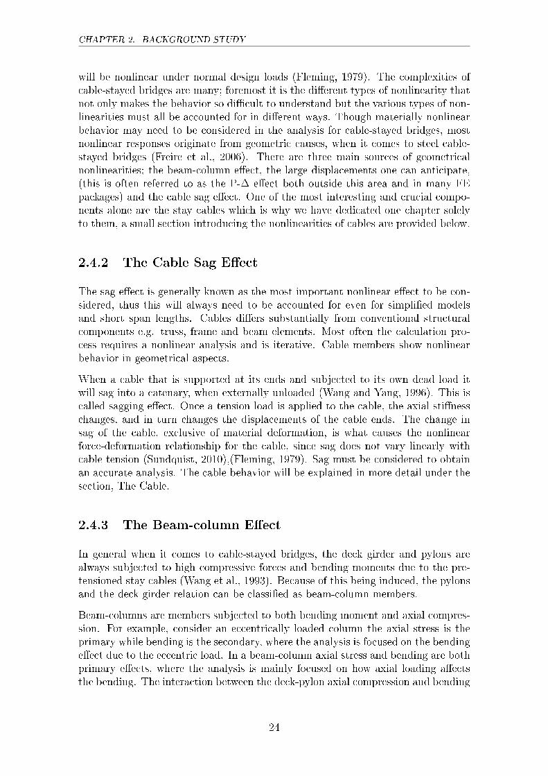
2.4.2 The Cable Sag E�ect
The sag e�ect is generally known as the most important nonlinear e�ect to be con-sidered, thus this will always need to be accounted for even for simpli�ed modelsand short span lengths. Cables di�ers substantially from conventional structuralcomponents e.g. truss, frame and beam elements. Most often the calculation pro-cess requires a nonlinear analysis and is iterative. Cable members show nonlinearbehavior in geometrical aspects.
When a cable that is supported at its ends and subjected to its own dead load itwill sag into a catenary, when externally unloaded (Wang and Yang, 1996). This iscalled sagging e�ect. Once a tension load is applied to the cable, the axial sti�nesschanges, and in turn changes the displacements of the cable ends. The change insag of the cable, exclusive of material deformation, is what causes the nonlinearforce-deformation relationship for the cable, since sag does not vary linearly withcable tension (Sundquist, 2010),(Fleming, 1979). Sag must be considered to obtainan accurate analysis. The cable behavior will be explained in more detail under thesection, The Cable.
2.4.3 The Beam-column E�ect
In general when it comes to cable-stayed bridges, the deck girder and pylons arealways subjected to high compressive forces and bending moments due to the pre-tensioned stay cables (Wang et al., 1993). Because of this being induced, the pylonsand the deck girder relation can be classi�ed as beam-column members.
Beam-columns are members subjected to both bending moment and axial compres-sion. For example, consider an eccentrically loaded column the axial stress is theprimary while bending is the secondary, where the analysis is focused on the bendinge�ect due to the eccentric load. In a beam-column axial stress and bending are bothprimary e�ects, where the analysis is mainly focused on how axial loading a�ectsthe bending. The interaction between the deck-pylon axial compression and bending
24
2.4. INTRODUCTION TO NONLINEARITY
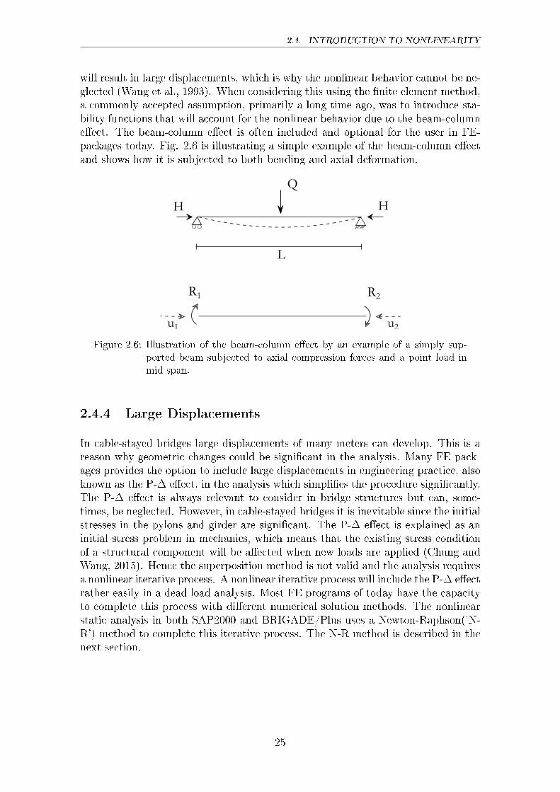
will result in large displacements, which is why the nonlinear behavior cannot be ne-glected (Wang et al., 1993). When considering this using the �nite element method,a commonly accepted assumption, primarily a long time ago, was to introduce sta-bility functions that will account for the nonlinear behavior due to the beam-columne�ect. The beam-column e�ect is often included and optional for the user in FE-packages today. Fig. 2.6 is illustrating a simple example of the beam-column e�ectand shows how it is subjected to both bending and axial deformation.
Q
H H
L
u1 u2
R1 R2
Figure 2.6: Illustration of the beam-column e�ect by an example of a simply sup-ported beam subjected to axial compression forces and a point load inmid span.
2.4.4 Large Displacements
In cable-stayed bridges large displacements of many meters can develop. This is areason why geometric changes could be signi�cant in the analysis. Many FE pack-ages provides the option to include large displacements in engineering practice, alsoknown as the P-� e�ect, in the analysis which simpli�es the procedure signi�cantly.The P-� e�ect is always relevant to consider in bridge structures but can, some-times, be neglected. However, in cable-stayed bridges it is inevitable since the initialstresses in the pylons and girder are signi�cant. The P-� e�ect is explained as aninitial stress problem in mechanics, which means that the existing stress conditionof a structural component will be a�ected when new loads are applied (Chung andWang, 2015). Hence the superposition method is not valid and the analysis requiresa nonlinear iterative process. A nonlinear iterative process will include the P-� e�ectrather easily in a dead load analysis. Most FE programs of today have the capacityto complete this process with di�erent numerical solution methods. The nonlinearstatic analysis in both SAP2000 and BRIGADE/Plus uses a Newton-Raphson('N-R') method to complete this iterative process. The N-R method is described in thenext section.
25
CHAPTER 2. BACKGROUND STUDY
2.4.5 Newton-Raphson Method
When analyzing the response of a structure that is exposed to a load we'll receive anonlinear force-deformation curve. The Newton-Raphson method is used for solvingequations numerically, and is based on linear approximations. The method is basedupon small changes that will make a non-linear equation linear by iterating a solutionin small steps (Chopra, 2012).
For a structure to be in static equilibrium that is exposed to an external force, thenet force acting on every node has to be zero, i.e. the external force, fe, and theinternal, resisting force, fs(u), have to be balanced according to:
fs(u) = fe (2.14)
Where fs,u andfe are vectors of n degrees of freedom. This non-linear equation fora static problem now has to be solved. We want to determine the deformation, u,caused by the external force fe . In order to �nd the displacement, we derive aniterative process to better estimate u(i+1) from a present guess to the solution u(i).To �nd this we use Taylors series:
f (j+1)s = f (j)s +@fs
@uju(j)
�u(j+1) � u(j)
�+
1
2
@2fs
@u2ju(j)
�u(j+1) � u(j)
�2+ ::: (2.15)
Here we can see that if �u is to be very small, i.e. the step increment is small, thenthe second order term, and the ones above that could be neglected. Doing so, thenonlinear equation now becomes linear:
f (j+1)s � f (j)s + k(j)T �u(j) = fe (2.16)
ork(j)T �u(j) = fe � f (j)s = R(j) (2.17)
where
k(j)T =
1
2
@2fs
@u2ju(j) (2.18)
The residual force, R(j), will give an additional displacement, that is used to solvethe next displacement step, u(j+1):
u(j+1) = u(j) +�u(j) (2.19)
Eq. (2.14) will normally not be ful�lled even after this correction. In order to �ndR(j+1) Eq. (2.17) is modi�ed to calculate its force R(j+1) = fe � f
(j+1)s . The same
process is repeated until the basic Eq. (2.14) is ful�lled with acceptable accuracy.
26
2.5. THE CABLE
Adding together the previous steps the iteration formulation is completed to �ndthe next displacement coordinate. With small increment steps, this procedure cangive an accurate re�ection of the nonlinear force-deformation curve.
2.5 The Cable
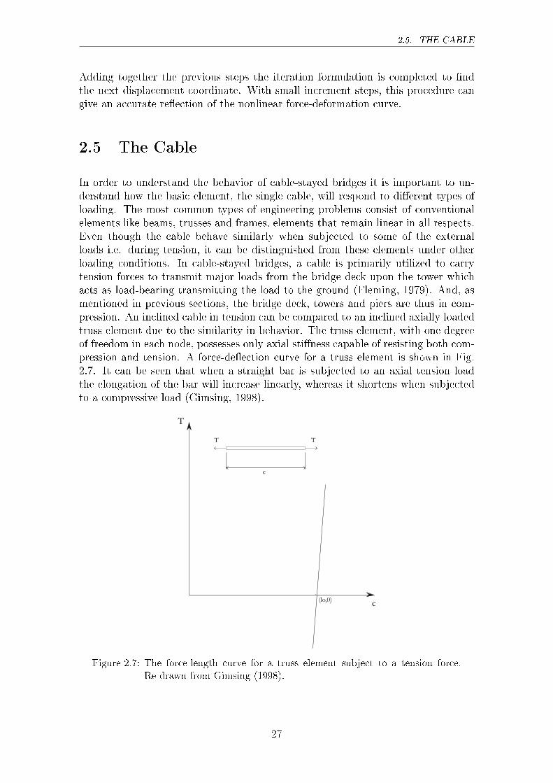
In order to understand the behavior of cable-stayed bridges it is important to un-derstand how the basic element, the single cable, will respond to di�erent types ofloading. The most common types of engineering problems consist of conventionalelements like beams, trusses and frames, elements that remain linear in all respects.Even though the cable behave similarly when subjected to some of the externalloads i.e. during tension, it can be distinguished from these elements under otherloading conditions. In cable-stayed bridges, a cable is primarily utilized to carrytension forces to transmit major loads from the bridge deck upon the tower whichacts as load-bearing transmitting the load to the ground (Fleming, 1979). And, asmentioned in previous sections, the bridge deck, towers and piers are thus in com-pression. An inclined cable in tension can be compared to an inclined axially loadedtruss element due to the similarity in behavior. The truss element, with one degreeof freedom in each node, possesses only axial sti�ness capable of resisting both com-pression and tension. A force-de�ection curve for a truss element is shown in Fig.2.7. It can be seen that when a straight bar is subjected to an axial tension loadthe elongation of the bar will increase linearly, whereas it shortens when subjectedto a compressive load (Gimsing, 1998).
T
c
T T
c
(lo,0)
Figure 2.7: The force-length curve for a truss element subject to a tension force.Re-drawn from Gimsing (1998).
27
CHAPTER 2. BACKGROUND STUDY
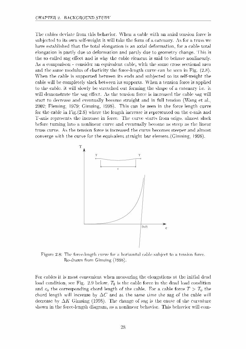
The cables deviate from this behavior. When a cable with an axial tension force issubjected to its own self-weight it will take the form of a catenary. As for a truss wehave established that the total elongation is an axial deformation, for a cable totalelongation is partly due to deformation and partly due to geometry change. This isthe so called sag e�ect and is why the cable element is said to behave nonlinearly.As a comparison - consider an equivalent cable, with the same cross sectional areaand the same modulus of elasticity the force-length curve can be seen in Fig. (2.8).When the cable is supported between its ends and subjected to its self-weight thecable will be completely slack between its supports. When a tension force is appliedto the cable, it will slowly be stretched out forming the shape of a catenary i.e. itwill demonstrate the sag e�ect. As the tension force is increased the cable sag willstart to decrease and eventually become straight and in full tension (Wang et al.,2002; Fleming, 1979; Gimsing, 1998). This can be seen in the force-length curvefor the cable in Fig.(2.8) where the length increase is represented on the c-axis andT-axis represents the increase in force. The curve starts from origo, almost slackbefore turning into a nonlinear curve and eventually become as steep as the lineartruss curve. As the tension force is increased the curve becomes steeper and almostconverge with the curve for the equivalent straight bar element.(Gimsing, 1998).
T
c
T T
c
(lo,0)
Figure 2.8: The force-length curve for a horizontal cable subject to a tension force.Re-drawn from Gimsing (1998).
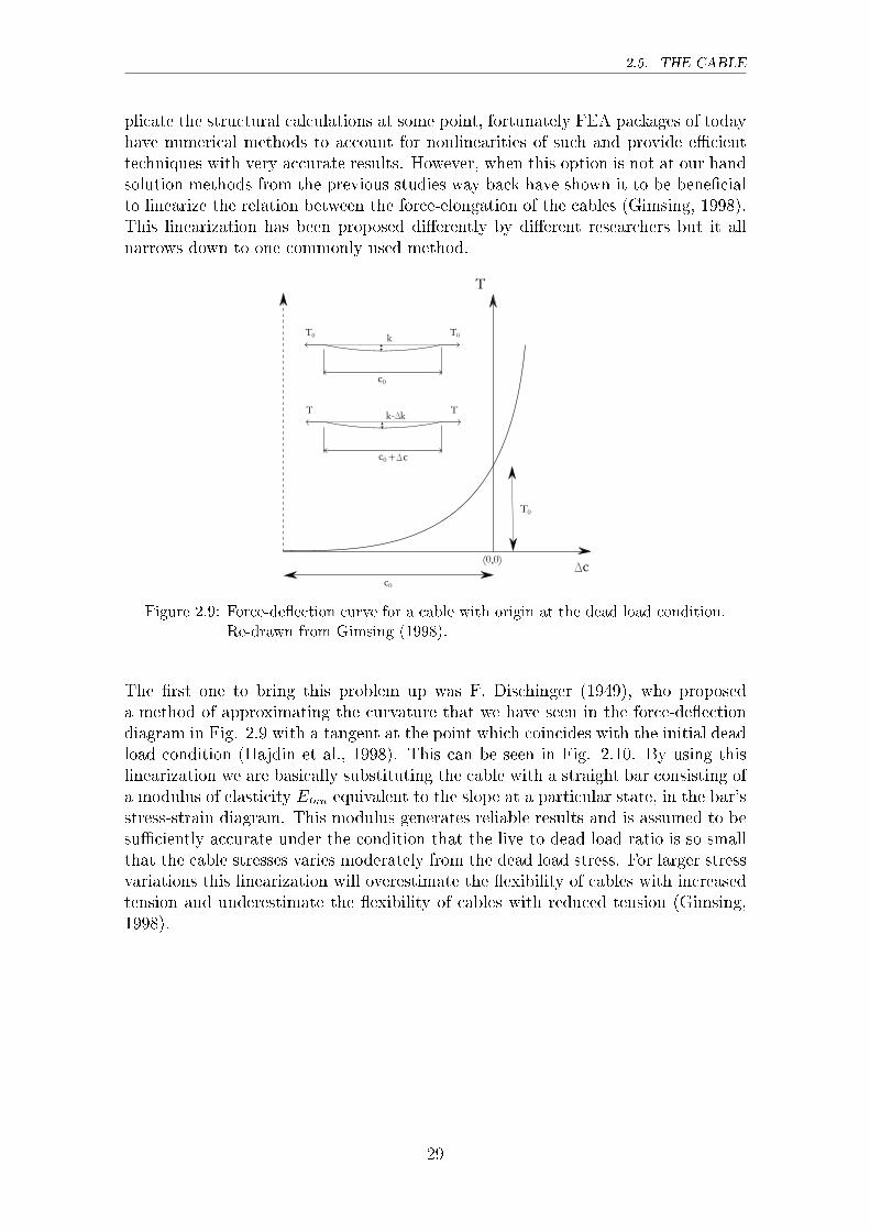
For cables it is most convenient when measuring the elongations at the initial deadload condition, see Fig. 2.9 below, T0 is the cable force in the dead load conditionand c0 the corresponding chord length of the cable. For a cable force T > T0 thechord length will increase by �C and at the same time the sag of the cable willdecrease by �K Gimsing (1998). The change of sag is the cause of the curvatureshown in the force-length diagram, as a nonlinear behavior. This behavior will com-
28
2.5. THE CABLE
plicate the structural calculations at some point, fortunately FEA packages of todayhave numerical methods to account for nonlinearities of such and provide e�cienttechniques with very accurate results. However, when this option is not at our handsolution methods from the previous studies way back have shown it to be bene�cialto linearize the relation between the force-elongation of the cables (Gimsing, 1998).This linearization has been proposed di�erently by di�erent researchers but it allnarrows down to one commonly used method.
T
c
T T
c0
k- k
T0 T0
c0
c0
+
k
(0,0)
D
D
D
c
T0
Figure 2.9: Force-de�ection curve for a cable with origin at the dead load condition.Re-drawn from Gimsing (1998).
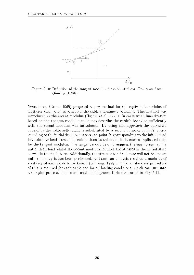
The �rst one to bring this problem up was F. Dischinger (1949), who proposeda method of approximating the curvature that we have seen in the force-de�ectiondiagram in Fig. 2.9 with a tangent at the point which coincides with the initial deadload condition (Hajdin et al., 1998). This can be seen in Fig. 2.10. By using thislinearization we are basically substituting the cable with a straight bar consisting ofa modulus of elasticity Etan equivalent to the slope at a particular state, in the bar'sstress-strain diagram. This modulus generates reliable results and is assumed to besu�ciently accurate under the condition that the live-to-dead load ratio is so smallthat the cable stresses varies moderately from the dead load stress. For larger stressvariations this linearization will overestimate the �exibility of cables with increasedtension and underestimate the �exibility of cables with reduced tension (Gimsing,1998).
29
CHAPTER 2. BACKGROUND STUDY
Etan1
A
B
s
d/
s1
s2
c
Figure 2.10: De�nition of the tangent modulus for cable sti�ness. Re-drawn fromGimsing (1998).
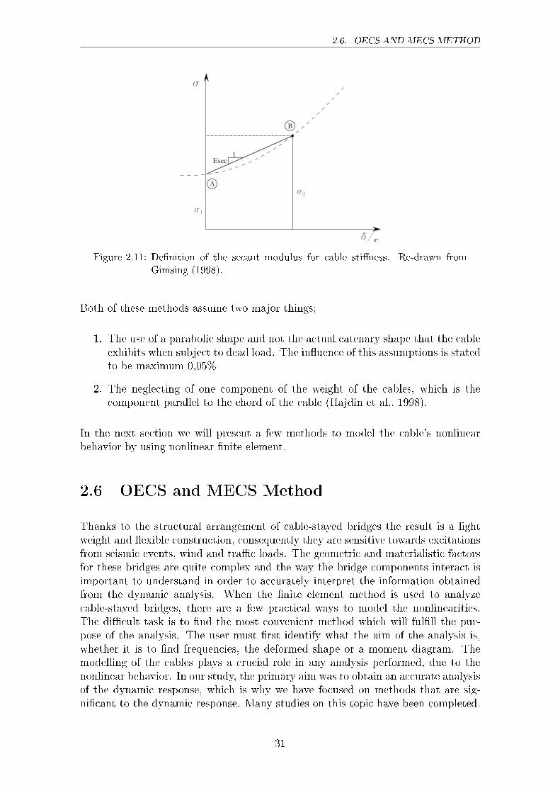
Years later, (Ernst, 1965) proposed a new method for the equivalent modulus ofelasticity that could account for the cable's nonlinear behavior. This method wasintroduced as the secant modulus (Hajdin et al., 1998). In cases when linearizationbased on the tangent modulus could not describe the cable's behavior su�cientlywell, the secant modulus was introduced. By using this approach the curvaturecaused by the cable self-weight is substituted by a secant between point A, corre-sponding to the initial dead load stress and point B, corresponding to the initial deadload plus live load stress. The calculations for this modulus is more complicated thanfor the tangent modulus. The tangent modulus only requires the equilibrium at theinitial dead load whilst the secant modulus requires the stresses in the initial stateas well in the �nal state. Additionally, the stress at the �nal state will not be knownuntil the analysis has been performed, and such an analysis requires a modulus ofelasticity of each cable to be known (Gimsing, 1998). Thus, an iterative procedureof this is required for each cable and for all loading conditions, which can turn intoa complex process. The secant modulus approach is demonstrated in Fig. 2.11.
30
2.6. OECS AND MECS METHOD
Esec1
A
B
s
d/
s1
s2
c
Figure 2.11: De�nition of the secant modulus for cable sti�ness. Re-drawn fromGimsing (1998).
Both of these methods assume two major things;
1. The use of a parabolic shape and not the actual catenary shape that the cableexhibits when subject to dead load. The in�uence of this assumptions is statedto be maximum 0,05%
2. The neglecting of one component of the weight of the cables, which is thecomponent parallel to the chord of the cable (Hajdin et al., 1998).
In the next section we will present a few methods to model the cable's nonlinearbehavior by using nonlinear �nite element.
2.6 OECS and MECS Method
Thanks to the structural arrangement of cable-stayed bridges the result is a lightweight and �exible construction, consequently they are sensitive towards excitationsfrom seismic events, wind and tra�c loads. The geometric and materialistic factorsfor these bridges are quite complex and the way the bridge components interact isimportant to understand in order to accurately interpret the information obtainedfrom the dynamic analysis. When the �nite element method is used to analyzecable-stayed bridges, there are a few practical ways to model the nonlinearities.The di�cult task is to �nd the most convenient method which will ful�ll the pur-pose of the analysis. The user must �rst identify what the aim of the analysis is,whether it is to �nd frequencies, the deformed shape or a moment diagram. Themodelling of the cables plays a crucial role in any analysis performed, due to thenonlinear behavior. In our study, the primary aim was to obtain an accurate analysisof the dynamic response, which is why we have focused on methods that are sig-ni�cant to the dynamic response. Many studies on this topic have been completed.
31
CHAPTER 2. BACKGROUND STUDY
In a study performed by Abdel-Gha�ar and Khalifa (1991), they demonstrated howdi�erent meshing schemes would generate di�erent mode shapes depending on thediscretization of the cables. They categorized the mode shapes attained into global,local and coupled modes (Liu et al., 2014). The global mode shapes are foremostdominated by deck-tower deformation with the cable deformation occurring slowlyenough to remain in internal equilibrium. The local modes are mainly by cablevibrations with negligible deck-tower deformation and the coupled modes have sig-ni�cant contributions from both cables and deck-tower system. This study was onceagain performed by (Au et al., 2001) when comparisons between two methods werecompleted. This is presented in more detail in our pre-study under the method.In the following sections we will introduce some of the relevant methods, and alsopresent the method of choice in our thesis.
2.6.1 OECS with an Equivalent Modulus of Elasticity
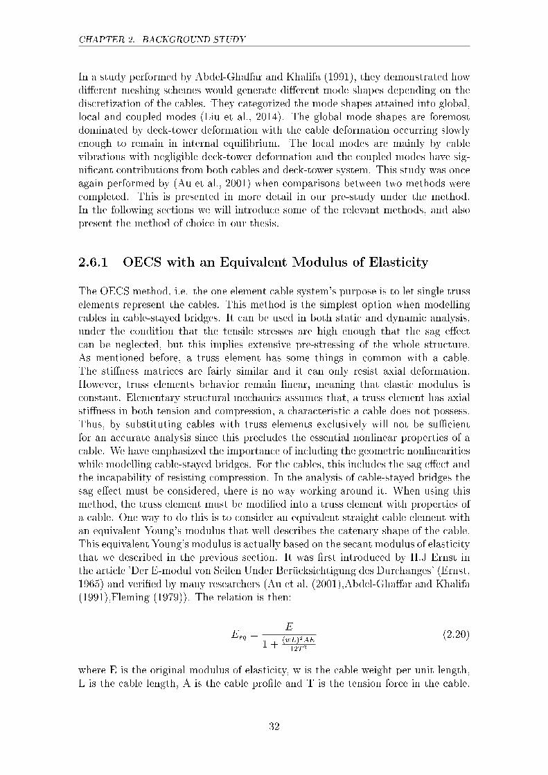
The OECS method, i.e. the one element cable system's purpose is to let single trusselements represent the cables. This method is the simplest option when modellingcables in cable-stayed bridges. It can be used in both static and dynamic analysis,under the condition that the tensile stresses are high enough that the sag e�ectcan be neglected, but this implies extensive pre-stressing of the whole structure.As mentioned before, a truss element has some things in common with a cable.The sti�ness matrices are fairly similar and it can only resist axial deformation.However, truss elements behavior remain linear, meaning that elastic modulus isconstant. Elementary structural mechanics assumes that, a truss element has axialsti�ness in both tension and compression, a characteristic a cable does not possess.Thus, by substituting cables with truss elements exclusively will not be su�cientfor an accurate analysis since this precludes the essential nonlinear properties of acable. We have emphasized the importance of including the geometric nonlinearitieswhile modelling cable-stayed bridges. For the cables, this includes the sag e�ect andthe incapability of resisting compression. In the analysis of cable-stayed bridges thesag e�ect must be considered, there is no way working around it. When using thismethod, the truss element must be modi�ed into a truss element with properties ofa cable. One way to do this is to consider an equivalent straight cable element withan equivalent Young's modulus that well describes the catenary shape of the cable.This equivalent Young's modulus is actually based on the secant modulus of elasticitythat we described in the previous section. It was �rst introduced by H.J Ernst inthe article 'Der E-modul von Seilen Under Berücksichtigung des Durchanges' (Ernst,1965) and veri�ed by many researchers (Au et al. (2001),Abdel-Gha�ar and Khalifa(1991),Fleming (1979)). The relation is then:
Eeq =E
1 + (wL)2AE12T 3
(2.20)
where E is the original modulus of elasticity, w is the cable weight per unit length,L is the cable length, A is the cable pro�le and T is the tension force in the cable.
32
2.6. OECS AND MECS METHOD
The equivalent modulus results in a length change for the cable, which is the samelength change as the one caused by the catenary shape induced by the self-weightand the extension e�ects in the actual cable. However, this method is based ona parabolic shape and not the actual catenary shape, which is only acceptable formoderate curvatures (Freire et al., 2006).
In Eq. (2.20) the e�ective material elastic modulus is applied and only an assumedcable pro�le needs to be inserted to account for the e�ect of cable sag. This methodis often used to model cables in cable-stayed bridges due to its ability to account forthe sag e�ect and the simplicity of using it. However, once the equivalent Young'smodulus has been obtained, the cable pro�le will not contribute to the analysis whichmeans that this method precludes transverse cable vibrations. In some studies thecable self-weight has been neglected to obtain constant tension forces during thestatic analysis. One could question whether this is accurate since the essential partof this method is to simulate the sag e�ect, but this is plausible since the equationis depending on the cable pro�le, tension force and the cable weight per unit length.This will automatically account for the sag e�ect in the context of static equilibrium,and in the analysis of vibrations when the cable's own vibration is of no interest.
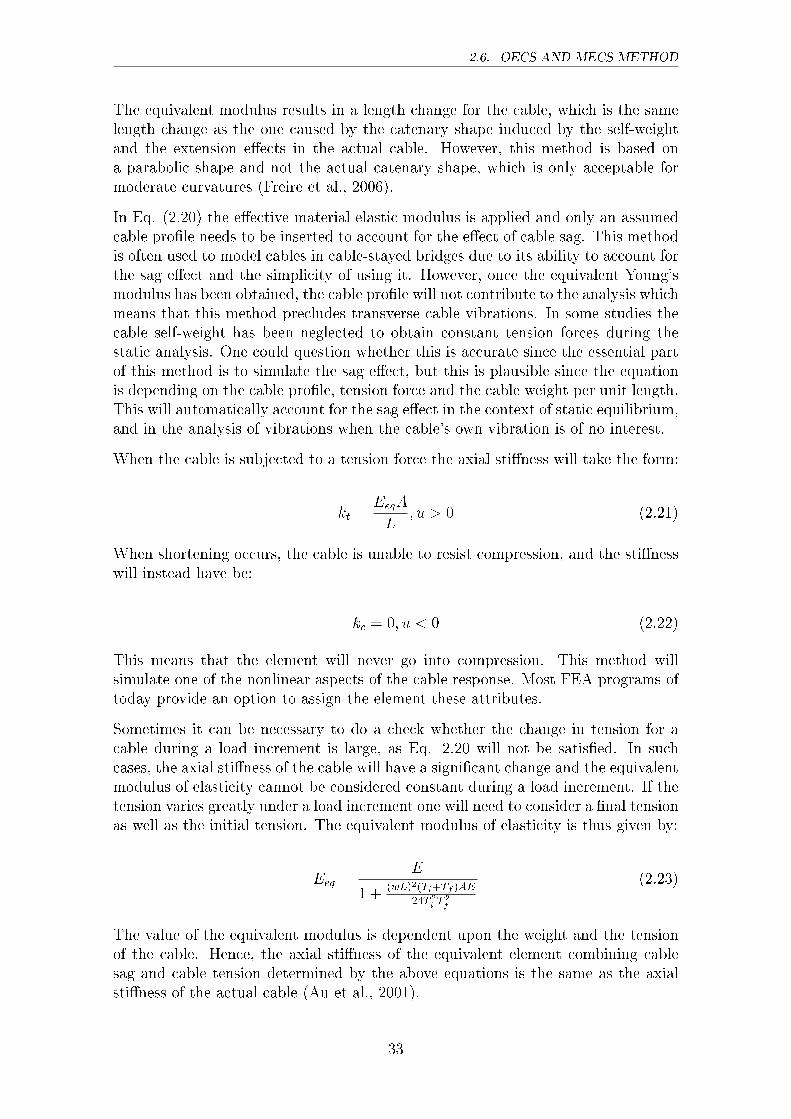
When the cable is subjected to a tension force the axial sti�ness will take the form:
kt =EeqA
L; u > 0 (2.21)
When shortening occurs, the cable is unable to resist compression, and the sti�nesswill instead have be:
kc = 0; u < 0 (2.22)
This means that the element will never go into compression. This method willsimulate one of the nonlinear aspects of the cable response. Most FEA programs oftoday provide an option to assign the element these attributes.
Sometimes it can be necessary to do a check whether the change in tension for acable during a load increment is large, as Eq. 2.20 will not be satis�ed. In suchcases, the axial sti�ness of the cable will have a signi�cant change and the equivalentmodulus of elasticity cannot be considered constant during a load increment. If thetension varies greatly under a load increment one will need to consider a �nal tensionas well as the initial tension. The equivalent modulus of elasticity is thus given by:
Eeq =E
1 +(wL)2(Ti+Tf )AE
24T 2i T
2f
(2.23)
The value of the equivalent modulus is dependent upon the weight and the tensionof the cable. Hence, the axial sti�ness of the equivalent element combining cablesag and cable tension determined by the above equations is the same as the axialsti�ness of the actual cable (Au et al., 2001).
33
CHAPTER 2. BACKGROUND STUDY
According to Abdel-Gha�ar and Khalifa (1991), this method is inadequate if onewants to capture all modes, the global and the cable vibrations which this methodwill preclude. However, sometimes it is not necessary to include the transversecable vibrations. This will depend on what the user wants to analyze. Whetherthis method is adequate needs to be evaluated before eliminating this option. Thisis up to the user to determine. Noteworthy, sometimes the equivalent elasticityis not required, it is recommended to �rst try with a mean modulus of elasticity,approximately 190-195 GPa and evaluate whether the tension and sag varies greatly(DelForno, 2001).
2.6.2 MECS with the Original Modulus of Elasticity
The MECS method is described as a cable system in which each cable is discretizedinto multiple elements to simulate the sag e�ect (Liu et al., 2014). Thus, whenusing this method, an equivalent modulus of elasticity is not necessary. The appliedmodulus of elasticity is instead the e�ective material modulus. It is a powerfulmethod as it accounts for the sag e�ect as well as includes transverse cable vibrationsproviding the possibility to obtain the coupled modes. Most of the studies foundwere completed using truss elements, when doing that the catenary shape cannot becorrectly simulated since truss elements can only resist axial deformation. Insteadthe appearing curvature will have small deviations in the multiple-straight link. Thismight be su�cient when performing a linear analysis, nonlinear analyses requiresother conditions.
When modelling the cables using beam elements these conditions can be ful�lled.Beam elements can represent a beam in bending, a truss or a torsion bar. Eventhough beam elements can resist bending, which in reality a cable can not do likea beam, this �exural rigidity is necessary to simulate the cable sag accurately. Thebending sti�ness allows the beam to bend due to its self weight, just like a cablesagging to its own self weight. This kind of behavior is di�cult to capture and canbe done best by modelling using beam elements. The bending and axial sti�nesscan carry the self weight and creates the sagging curve more accurately after thediscretization of the cable.
It is essential that the end of the cables have been assigned moment end releasessince the cable cannot transmit moments in the cable ends. This is not requiredwhen modelling using truss elements, resisting only axial deformation, but sincebeam elements are capable to resist bending and axial deformation, this will needto be recti�ed. Additionally, there are some bending forces in the cable that can notbe captured by modelling using truss elements.
When modelling cables, the sag e�ect must be considered and it is recommended thatthe equivalent Young's modulus is calculated for each cable if not nonlinear elementsare used. For the analysis performed in the thesis we have chosen to use the MECSmethod with beam elements to reduce the calculations of an equivalent modulus ofelasticity that would become individual for each cable, which was evaluated to bemore time consuming. The MECS method was found the simplest fastest method
34
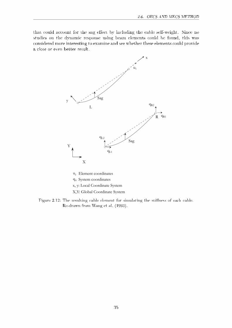
2.6. OECS AND MECS METHOD
that could account for the sag e�ect by including the cable self-weight. Since nostudies on the dynamic response using beam elements could be found, this wasconsidered more interesting to examine and see whether these elements could providea close or even better result.
L
y
x
u1
Sag
Sag
R
qL2
qL1
qR2
qR1
Y
X
uj: Element coordinatesqx: System coordinates
x, y: Local Coordinate System
X,Y: Global Coordinate System
Figure 2.12: The resulting cable element for simulating the sti�ness of each cable.Re-drawn from Wang et al. (1993).
35

Chapter 3
Method
3.1 Prestudy
3.1.1 Literature Example
In order to increase our knowledge and understanding of how to model cable-stayedbridges and cable elements, a pre-study on these topics were completed. In orderto get to know the two software, SAP2000 and BRIGADE/Plus, we needed to �ndreports in which they examined and modelled very basic cable-stayed bridges, withresults provided in the report, in order to practise on. Such an exercise examplewas found in the report 'On the Determination of Natural Frequencies and ModeShapes of Cable-stayed Bridges' (Au et al., 2001).
The paper presents two ways of modelling cables to compare the two and analyzewhich one that generates the most accurate results (Au et al., 2001). It startsby presenting the common way to model cable-stayed bridges, using single trusselements with an equivalent modulus of elasticity with the ability of allowing forsag, when modelling cables. This comparisson was made due to the study performedby Abdel-Gha�ar and Khalifa (1991) that we mentioned shortly under the sectionOECS and MECS Method. They showed that according to their study, the OECSmethod did not generate accurate results. They concluded that this way of modellingstay cables is inadequate for an accurate dynamic analysis due to the exclusion ofthe transverse cable vibrations. The OECS method has been used for years, but asmore extravagant and slender structures are being built, it is necessary to becomemore close to reality when performing analyses. This method is simple and generatesclose results. It may be used when transverse cable vibrations are not essential forthe analysis, but it is important to acknowledge that many modes will be excludedin the analysis. This method can pick up the global modes but precludes the localcable vibration and thus the coupled modes. By subdividing the cables we receivemode shapes and frequencies of the cable movement that we exclude when modellingwith a single truss element. These two methods are compared and analyzed by (Auet al., 2001).
37
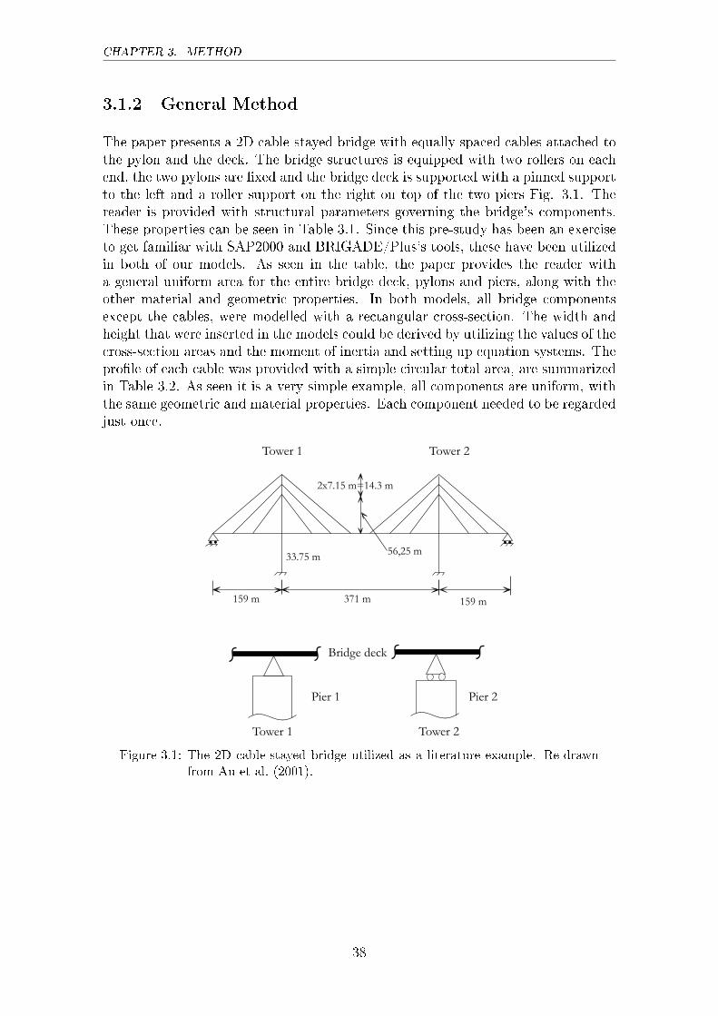
CHAPTER 3. METHOD
3.1.2 General Method
The paper presents a 2D cable-stayed bridge with equally spaced cables attached tothe pylon and the deck. The bridge structures is equipped with two rollers on eachend, the two pylons are �xed and the bridge deck is supported with a pinned supportto the left and a roller support on the right on top of the two piers Fig. 3.1. Thereader is provided with structural parameters governing the bridge's components.These properties can be seen in Table 3.1. Since this pre-study has been an exerciseto get familiar with SAP2000 and BRIGADE/Plus's tools, these have been utilizedin both of our models. As seen in the table, the paper provides the reader witha general uniform area for the entire bridge deck, pylons and piers, along with theother material and geometric properties. In both models, all bridge componentsexcept the cables, were modelled with a rectangular cross-section. The width andheight that were inserted in the models could be derived by utilizing the values of thecross-section areas and the moment of inertia and setting up equation systems. Thepro�le of each cable was provided with a simple circular total area, are summarizedin Table 3.2. As seen it is a very simple example, all components are uniform, withthe same geometric and material properties. Each component needed to be regardedjust once.
Bridge deck
Tower 1 Tower 2
Pier 1 Pier 2
Tower 1 Tower 2
2x7.15 m=14.3 m
33.75 m 56,25 m
371 m159 m 159 m
Figure 3.1: The 2D cable-stayed bridge utilized as a literature example. Re-drawnfrom Au et al. (2001).
38
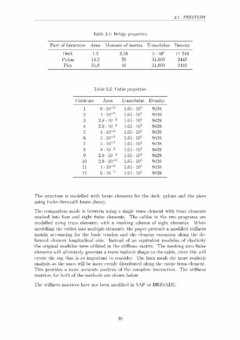
3.1. PRESTUDY
Table 3.1: Bridge properties
Part of Structure Area Moment of inertia E-modulus Density
Deck 1:2 2:58 2 � 105 11 244Pylon 14:2 30 31;600 2449Pier 35:8 40 31;600 2449
Table 3.2: Cable properties
Cable.no Area E-modulus Density
1 6 � 10�2 1:65 � 105 94382 4 � 10�2 1:65 � 105 94383 2:8 � 10�2 1:65 � 105 94384 2:8 � 10�2 1:65 � 105 94385 4 � 10�2 1:65 � 105 94386 5 � 10�2 1:65 � 105 94387 5 � 10�2 1:65 � 105 94388 4 � 10�2 1:65 � 105 94389 2:8 � 10�2 1:65 � 105 943810 2:8 � 10�2 1:65 � 105 943811 4 � 10�2 1:65 � 105 943812 6 � 10�2 1:65 � 105 9438
The structure is modelled with beam elements for the deck, pylons and the piersusing Euler-Bernoulli beam theory.
The comparison made is between using a single truss element with truss elementsmeshed into four and eight �nite elements. The cables in the two programs aremodelled using truss elements with a meshing scheme of eight elements. Whenmodelling the cables into multiple elements, the paper presents a modi�ed sti�nessmatrix accounting for the basic tension and the element extension along the de-formed element longitudinal axis. Instead of an equivalent modulus of elasticitythe original modulus were utilized in the sti�ness matrix. The meshing into �niteelements will ultimately generate a more realistic shape to the cable, since this willcreate the sag that is so important to consider. The �ner mesh the more realisticanalysis as the mass will be more evenly distributed along the entire truss element.This provides a more accurate analysis of the complete interaction. The sti�nessmatrices for both of the methods are shown below.
The sti�ness matrices have not been modi�ed in SAP or BRIGADE.
39
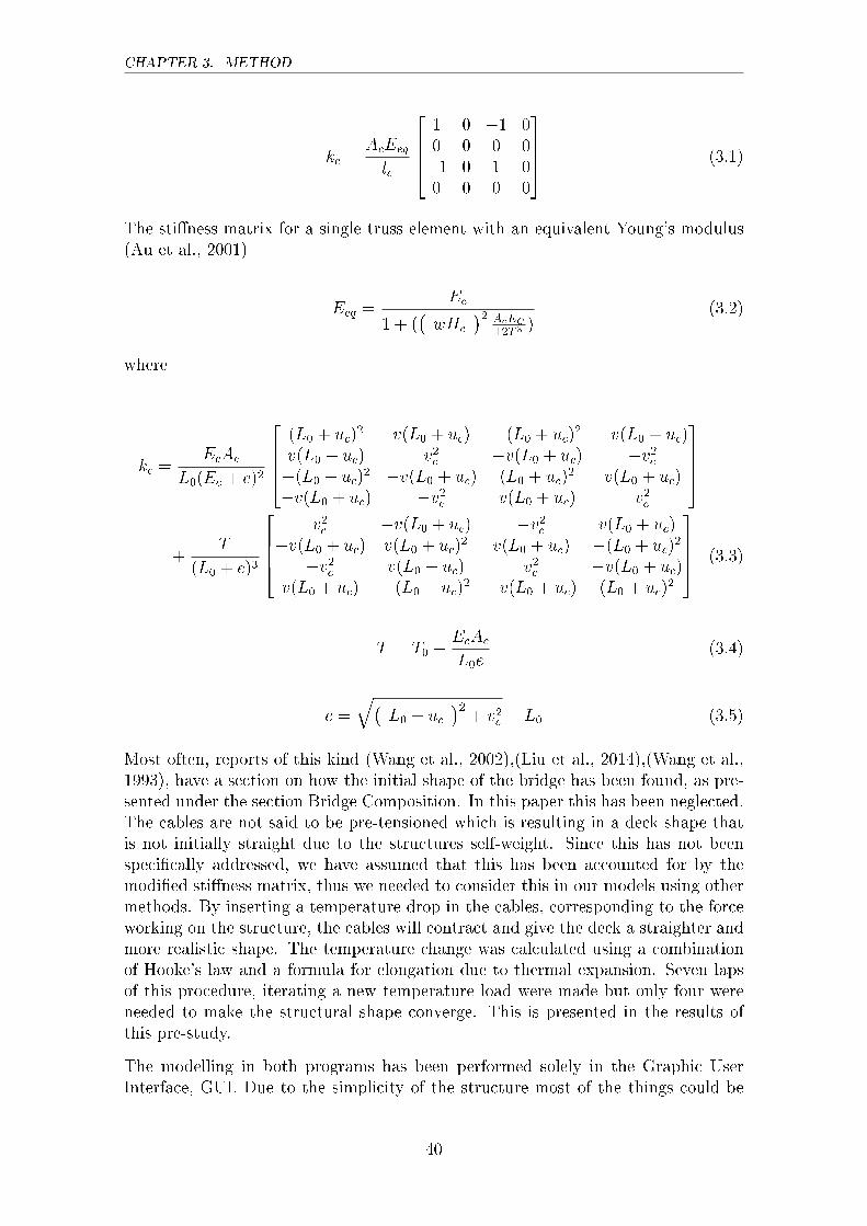
CHAPTER 3. METHOD
kc =AcEeq
lc
2664
1 0 �1 00 0 0 0�1 0 1 00 0 0 0
3775 (3.1)
The sti�ness matrix for a single truss element with an equivalent Young's modulus(Au et al., 2001)
Eeq =Ec
1 + (�wHc
�2 AcEC12T 3 )
(3.2)
where
kc =EcAc
L0(Ec + e)2
2664
(L0 + uc)2 v(L0 + uc) �(L0 + uc)
2 �v(L0 + uc)v(L0 + uc) v2c �v(L0 + uc) �v2c�(L0 + uc)
2 �v(L0 + uc) (L0 + uc)2 v(L0 + uc)
�v(L0 + uc) �v2c v(L0 + uc) v2c
3775
+T
(L0 + e)3
2664
v2c �v(L0 + uc) �v2c v(L0 + uc)�v(L0 + uc) v(L0 + uc)
2 v(L0 + uc) �(L0 + uc)2
�v2c v(L0 + uc) v2c �v(L0 + uc)v(L0 + uc) �(L0 + uc)
2 �v(L0 + uc) (L0 + uc)2
3775 (3.3)
T = T0 +EcAc
L0e(3.4)
e =
q�L0 + uc
�2+ v2c � L0 (3.5)
Most often, reports of this kind (Wang et al., 2002),(Liu et al., 2014),(Wang et al.,1993), have a section on how the initial shape of the bridge has been found, as pre-sented under the section Bridge Composition. In this paper this has been neglected.The cables are not said to be pre-tensioned which is resulting in a deck shape thatis not initially straight due to the structures self-weight. Since this has not beenspeci�cally addressed, we have assumed that this has been accounted for by themodi�ed sti�ness matrix, thus we needed to consider this in our models using othermethods. By inserting a temperature drop in the cables, corresponding to the forceworking on the structure, the cables will contract and give the deck a straighter andmore realistic shape. The temperature change was calculated using a combinationof Hooke's law and a formula for elongation due to thermal expansion. Seven lapsof this procedure, iterating a new temperature load were made but only four wereneeded to make the structural shape converge. This is presented in the results ofthis pre-study.
The modelling in both programs has been performed solely in the Graphic UserInterface, GUI. Due to the simplicity of the structure most of the things could be
40
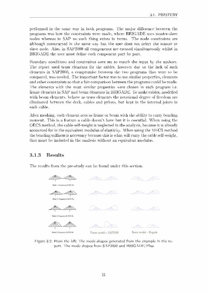
3.1. PRESTUDY
performed in the same way in both programs. The major di�erence between theprograms was how the constraints were made, where BRIGADE uses master-slavenodes whereas in SAP no such thing exists in terms. The node constraints arealthough constructed in the same way but the user does not select the master orslave node. Also, in SAP2000 all components are created simultaneously whilst inBRIGADE the user must de�ne each component part by part.
Boundary conditions and constraints were set to match the input by the authors.The report used truss elements for the cables, however due to the lack of suchelements in SAP2000, a compromise between the two programs that were to becompared, was needed. The important factor was to use similar properties, elementsand other constraints so that a fair comparison between the programs could be made.The elements with the most similar properties were chosen in each program i.e.frame elements in SAP and beam elements in BRIGADE. To make cables, modelledwith beam elements, behave as truss elements the rotational degree of freedom areeliminated between the deck, cables and pylons, but kept in the internal joints ineach cable.
After meshing, each element acts as frame or beam with the ability to carry bendingmoment. This is a feature a cable doesn't have but it is essential. When using theOECS method, the cable self-weight is neglected in the analysis, because it is alreadyaccounted for in the equivalent modulus of elasticity. When using the MECS methodthe bending sti�ness is necessary because this is what will carry the cable self-weight,that must be included in the analysis without an equivalent modulus.
3.1.3 Results
The results from the pre-study can be found under this section.
Figure 3.2: From the left; The mode shapes generated from the example in the re-port. The mode shapes from SAP2000 and BRIGADE/Plus.
41
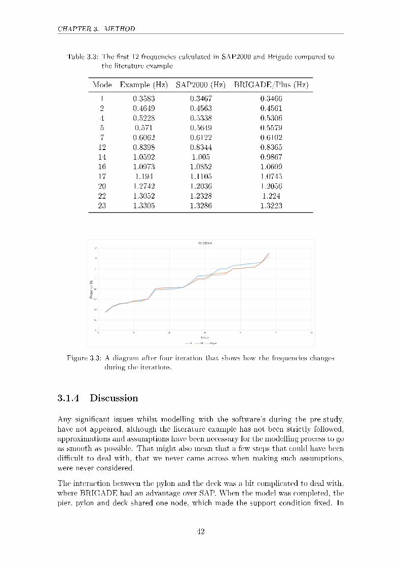
CHAPTER 3. METHOD
Table 3.3: The �rst 12 frequencies calculated in SAP2000 and Brigade compared tothe literature example
Mode Example (Hz) SAP2000 (Hz) BRIGADE/Plus (Hz)
1 0.3583 0.3467 0.34662 0.4649 0.4563 0.45614 0.5228 0.5338 0.53065 0.571 0.5649 0.55797 0.6062 0.6122 0.610212 0.8398 0.8344 0.836514 1.0592 1.005 0.986716 1.0973 1.0852 1.069917 1.194 1.1105 1.074520 1.2742 1.2036 1.205622 1.3052 1.2328 1.22423 1.3305 1.3286 1.3223
Figure 3.3: A diagram after four iteration that shows how the frequencies changesduring the iterations.
3.1.4 Discussion
Any signi�cant issues whilst modelling with the software's during the pre-study,have not appeared, although the literature example has not been strictly followed,approximations and assumptions have been necessary for the modelling process to goas smooth as possible. That might also mean that a few steps that could have beendi�cult to deal with, that we never came across when making such assumptions,were never considered.
The interaction between the pylon and the deck was a bit complicated to deal with,where BRIGADE had an advantage over SAP. When the model was completed, thepier, pylon and deck shared one node, which made the support condition �xed. In
42
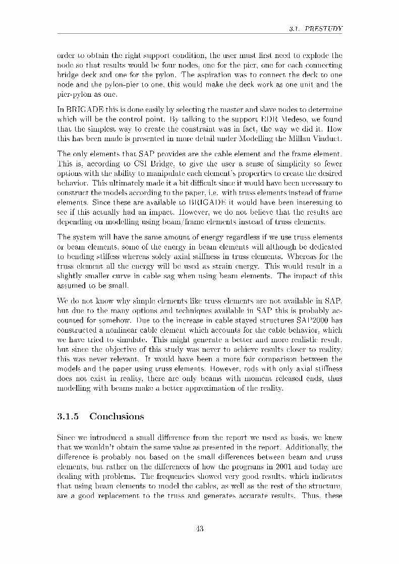
3.1. PRESTUDY
order to obtain the right support condition, the user must �rst need to explode thenode so that results would be four nodes, one for the pier, one for each connectingbridge deck and one for the pylon. The aspiration was to connect the deck to onenode and the pylon-pier to one, this would make the deck work as one unit and thepier-pylon as one.
In BRIGADE this is done easily by selecting the master and slave nodes to determinewhich will be the control point. By talking to the support EDR Medeso, we foundthat the simplest way to create the constraint was in fact, the way we did it. Howthis has been made is presented in more detail under Modelling the Millau Viaduct.
The only elements that SAP provides are the cable element and the frame element.This is, according to CSI Bridge, to give the user a sense of simplicity so feweroptions with the ability to manipulate each element's properties to create the desiredbehavior. This ultimately made it a bit di�cult since it would have been necessary toconstruct the models according to the paper, i.e. with truss elements instead of frameelements. Since these are available to BRIGADE it would have been interesting tosee if this actually had an impact. However, we do not believe that the results aredepending on modelling using beam/frame elements instead of truss elements.
The system will have the same amount of energy regardless if we use truss elementsor beam elements, some of the energy in beam elements will although be dedicatedto bending sti�ess whereas solely axial sti�ness in truss elements. Whereas for thetruss element all the energy will be used as strain energy. This would result in aslightly smaller curve in cable sag when using beam elements. The impact of thisassumed to be small.
We do not know why simple elements like truss elements are not available in SAP,but due to the many options and techniques available in SAP this is probably ac-counted for somehow. Due to the increase in cable-stayed structures SAP2000 hasconstructed a nonlinear cable element which accounts for the cable behavior, whichwe have tried to simulate. This might generate a better and more realistic result,but since the objective of this study was never to achieve results closer to reality,this was never relevant. It would have been a more fair comparison between themodels and the paper using truss elements. However, rods with only axial sti�nessdoes not exist in reality, there are only beams with moment released ends, thusmodelling with beams make a better approximation of the reality.
3.1.5 Conclusions
Since we introduced a small di�erence from the report we used as basis, we knewthat we wouldn't obtain the same value as presented in the report. Additionally, thedi�erence is probably not based on the small di�erences between beam and trusselements, but rather on the di�erences of how the programs in 2001 and today aredealing with problems. The frequencies showed very good results, which indicatesthat using beam elements to model the cables, as well as the rest of the structure,are a good replacement to the truss and generates accurate results. Thus, these
43
CHAPTER 3. METHOD
elements have been assessed appropriate to model the Millau Viaduct.
3.2 Modelling the Millau Viaduct
3.2.1 Bridge properties
All data necessary in order to calculate the second moments of inertia are obtainedfrom the drawings of the Millau viaduct provided by the head designer and engineer,Mr Michel Virlogeux in cooperation with Claude Servant, Ei�age Group, Vincent deVille and Jean-Yves Del Forno, Greisch. A complete edition of the drawings couldnot be provided, however a su�cient number of the most relevant drawings for themodelling to be completed were delivered.
The bridge's components consist of many complex details ful�lling both its archi-tectural and engineering purpose. The bridge composition was explained brie�y inthe introduction. A description on how the bridge properties have been simpli�edand calculated are presented stepwise in the following sections.
3.2.2 Material Properties
The steel grades in the steel materials of the Millau Viaduct varies from S355-S460.The advantage of steel materials is that the modulus of elasticity and density is aboutthe same value for conventional steel grades generally utilized in steel constructionsof today, unless the steel are supposed to be utilized for a speci�c purpose for instancein cables. However, this simpli�ed the procedure of assigning the steel material tothe entire deck.
The E-modulus for deck and pylons were set to 210 GPa. As for the cables, wenoted in previous sections that the steel utilized is of high strength and hence thematerial for the cables has to be accounted for individually. The properties of thecables are provided by Michel Virlogeux, the Guaranteed Ultimate Tensile Stress(GUTS) for the cables utilized to lift the bridge are fs=1860 MPa. The cables aremade of parallel individually protected strands, each strand has an area of 150 mm2
and consists of seven wires and the number of strands varies between 45-91 strandsdepending on its location. For such strands the E-modulus was set as 195 GPa.
Since no data on the piers except the cross-section or the formation longitudinallycould be provided, we had to assume a reasonable value for the reinforced concrete.Due to the size of the structure, the height of the piers and the way they had towithstand loads we assumed a dense reinforcement and applied a standard value ofreinforced concrete of 2500 kg/m3, the thermal coe�cient, the modulus of elasticityand Poission's ratio were also chosen as standard values of 9:8 � 10�6, 30 GPa and0.2.
44
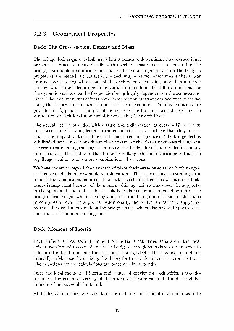
3.2. MODELLING THE MILLAU VIADUCT
3.2.3 Geometrical Properties
Deck; The Cross section, Density and Mass
The bridge deck is quite a challenge when it comes to determining its cross sectionalproperties. Since so many details with speci�c measurements are governing thebridge, reasonable assumptions on what will have a larger impact on the bridge'sproperties are needed. Fortunately, the deck is symmetric, which means that it wasonly necessary to regard one half of the deck when calculating, and then multiplythis by two. These calculations are essential to include in the sti�ness and mass forthe dynamic analysis, as the frequencies being highly dependent on the sti�ness andmass. The local moments of inertia and cross section areas are derived with Mathcadusing the theory for thin walled open steel cross sections. These calculations areprovided in Appendix. The global moments of inertia have been derived by thesummation of each local moment of inertia using Microsoft Excel.
The actual deck is provided with a truss and a diaphragm at every 4.17 m. Thesehave been completely neglected in the calculations as we believe that they have asmall or no impact on the sti�ness and thus the eigenfrequencies. The bridge deck issubdivided into 116 sections due to the variation of the plate thicknesses throughoutthe cross section along the length. In reality, the bridge deck is subdivided into manymore sections. This is due to that the bottom �ange thickness varies more than thetop �ange, which creates more combinations of sections.
We have chosen to regard the variation of plate thicknesses as equal on both �anges,as this seemed like a reasonable simpli�cation. This is less time consuming as itreduces the calculations required. The deck is so slender that this variation of thick-nesses is important because of the moment shifting various times over the supports,in the spans and under the cables. This is explained by a moment diagram of thebridge's dead weight, where the diagram shifts from being under tension in the spansto compression over the supports. Additionally, the bridge is elastically supportedby the cables continuously along the bridge length, which also has an impact on thetransitions of the moment diagram.
Deck; Moment of Inertia
Each sti�ener's local second moment of inertia is calculated separately, the localaxis is transformed to coincide with the bridge deck's global axis system in order tocalculate the total moment of inertia for the bridge deck. This has been completedmanually in Mathcad by utilizing the theory for thin walled open steel cross sections.The equations for the calculations are presented in Appendix.
Once the local moment of inertia and centre of gravity for each sti�ener was de-termined, the centre of gravity of the bridge deck were calculated and the globalmoment of inertia could be found.
All bridge components were calculated individually and thereafter summarized into
45
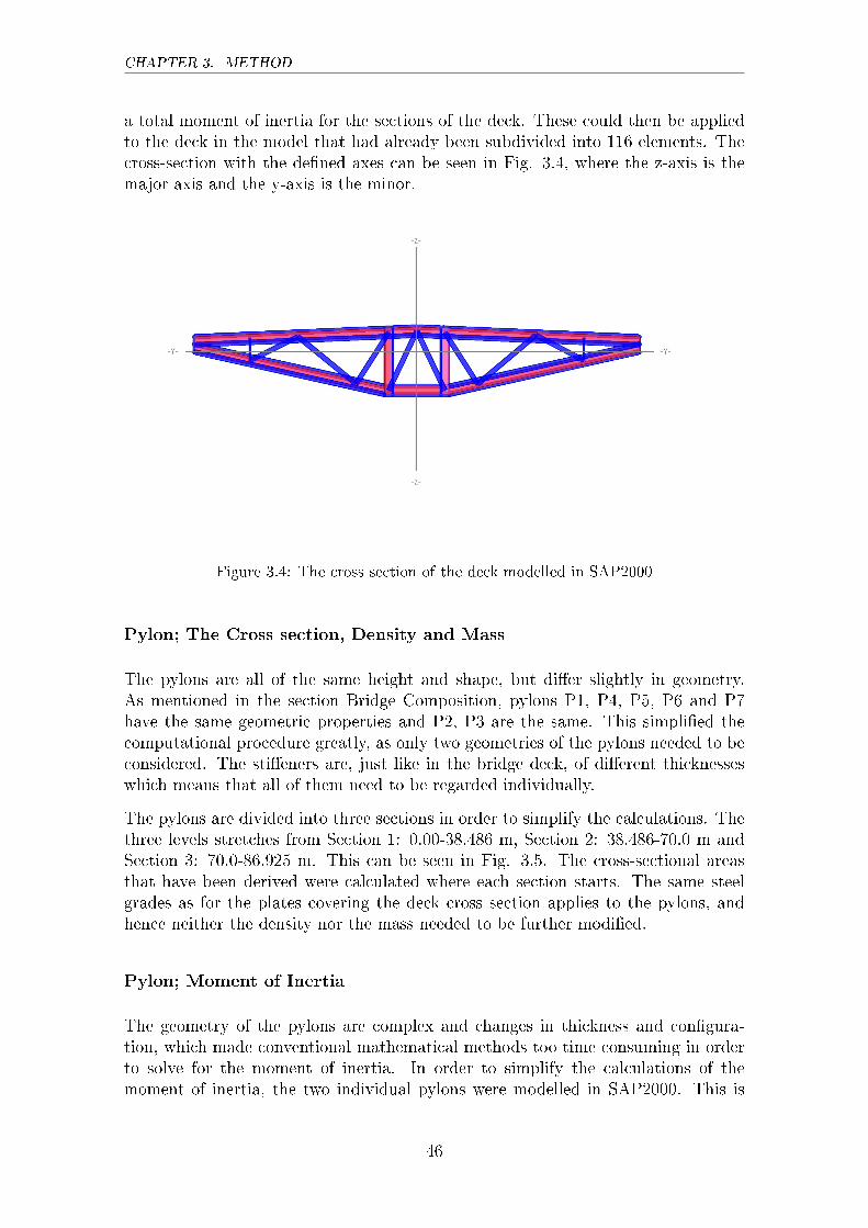
CHAPTER 3. METHOD
a total moment of inertia for the sections of the deck. These could then be appliedto the deck in the model that had already been subdivided into 116 elements. Thecross-section with the de�ned axes can be seen in Fig. 3.4, where the z-axis is themajor axis and the y-axis is the minor.
Figure 3.4: The cross section of the deck modelled in SAP2000
Pylon; The Cross section, Density and Mass
The pylons are all of the same height and shape, but di�er slightly in geometry.As mentioned in the section Bridge Composition, pylons P1, P4, P5, P6 and P7have the same geometric properties and P2, P3 are the same. This simpli�ed thecomputational procedure greatly, as only two geometries of the pylons needed to beconsidered. The sti�eners are, just like in the bridge deck, of di�erent thicknesseswhich means that all of them need to be regarded individually.
The pylons are divided into three sections in order to simplify the calculations. Thethree levels stretches from Section 1: 0.00-38.486 m, Section 2: 38.486-70.0 m andSection 3: 70.0-86.925 m. This can be seen in Fig. 3.5. The cross-sectional areasthat have been derived were calculated where each section starts. The same steelgrades as for the plates covering the deck cross section applies to the pylons, andhence neither the density nor the mass needed to be further modi�ed.
Pylon; Moment of Inertia
The geometry of the pylons are complex and changes in thickness and con�gura-tion, which made conventional mathematical methods too time consuming in orderto solve for the moment of inertia. In order to simplify the calculations of themoment of inertia, the two individual pylons were modelled in SAP2000. This is
46
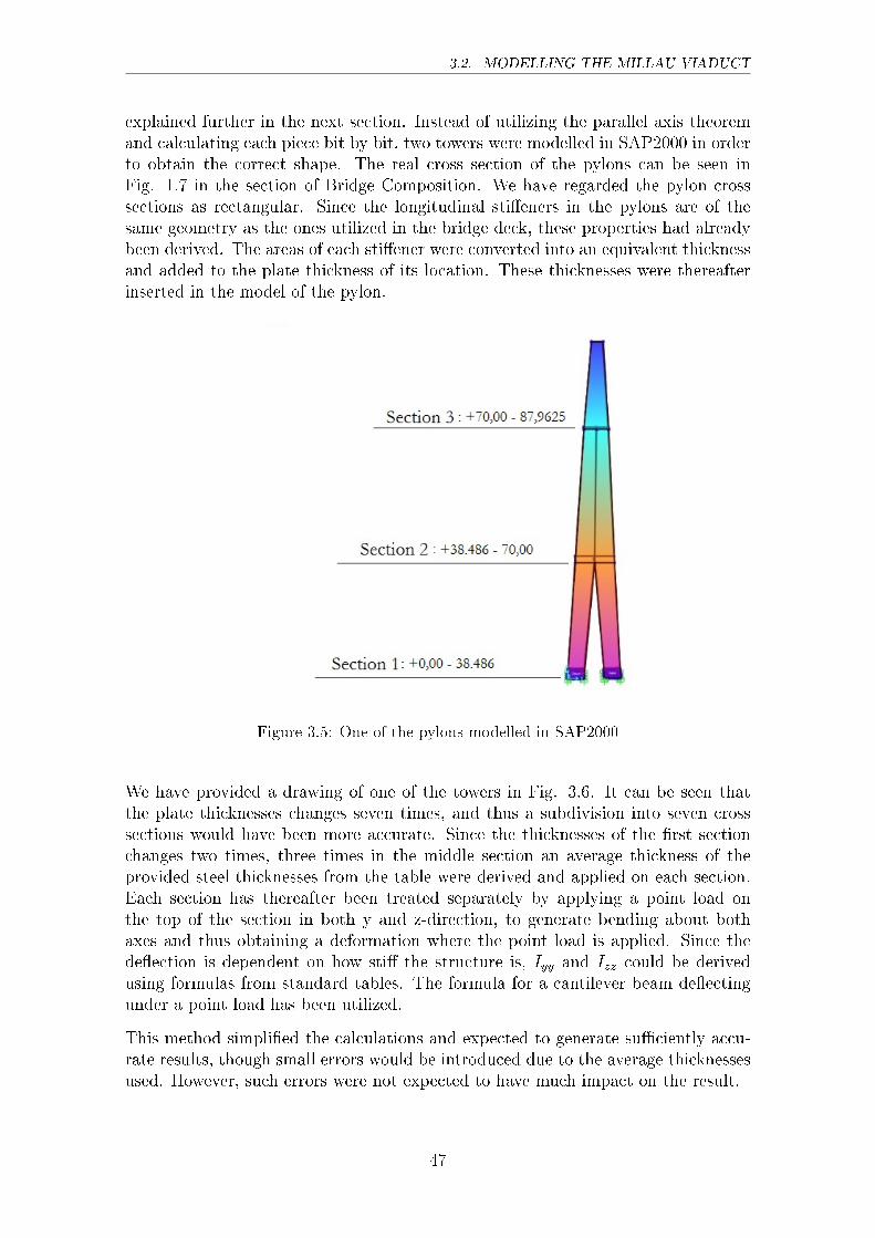
3.2. MODELLING THE MILLAU VIADUCT
explained further in the next section. Instead of utilizing the parallel axis theoremand calculating each piece bit by bit, two towers were modelled in SAP2000 in orderto obtain the correct shape. The real cross section of the pylons can be seen inFig. 1.7 in the section of Bridge Composition. We have regarded the pylon crosssections as rectangular. Since the longitudinal sti�eners in the pylons are of thesame geometry as the ones utilized in the bridge deck, these properties had alreadybeen derived. The areas of each sti�ener were converted into an equivalent thicknessand added to the plate thickness of its location. These thicknesses were thereafterinserted in the model of the pylon.
Figure 3.5: One of the pylons modelled in SAP2000
We have provided a drawing of one of the towers in Fig. 3.6. It can be seen thatthe plate thicknesses changes seven times, and thus a subdivision into seven crosssections would have been more accurate. Since the thicknesses of the �rst sectionchanges two times, three times in the middle section an average thickness of theprovided steel thicknesses from the table were derived and applied on each section.Each section has thereafter been treated separately by applying a point load onthe top of the section in both y and z-direction, to generate bending about bothaxes and thus obtaining a deformation where the point load is applied. Since thede�ection is dependent on how sti� the structure is, Iyy and Izz could be derivedusing formulas from standard tables. The formula for a cantilever beam de�ectingunder a point load has been utilized.
This method simpli�ed the calculations and expected to generate su�ciently accu-rate results, though small errors would be introduced due to the average thicknessesused. However, such errors were not expected to have much impact on the result.
47
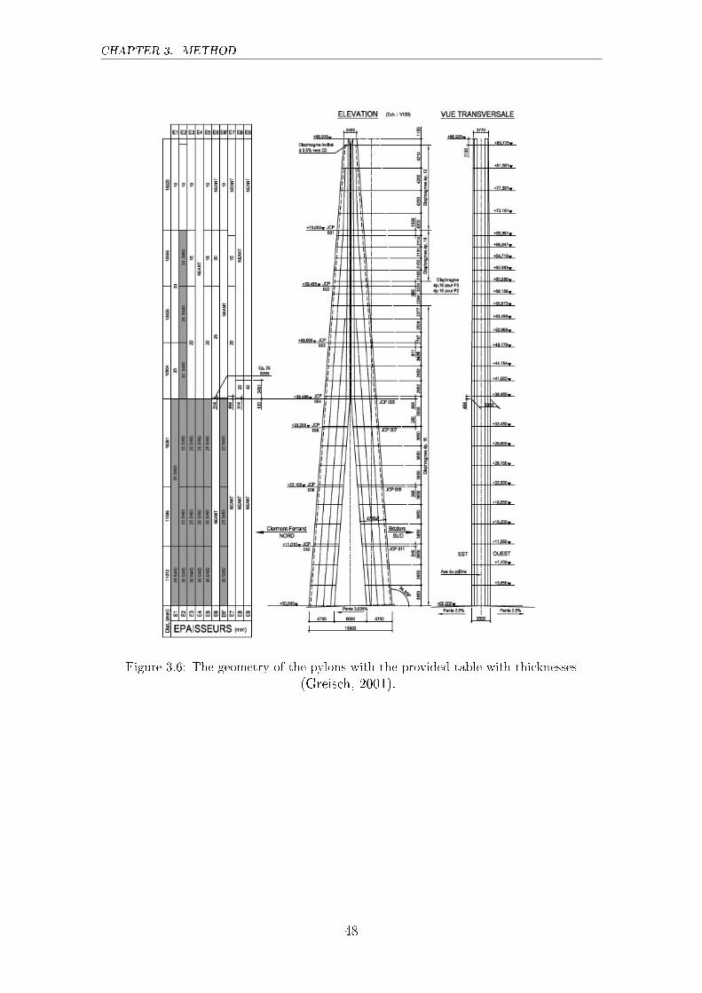
CHAPTER 3. METHOD
Figure 3.6: The geometry of the pylons with the provided table with thicknesses
(Greisch, 2001).
48
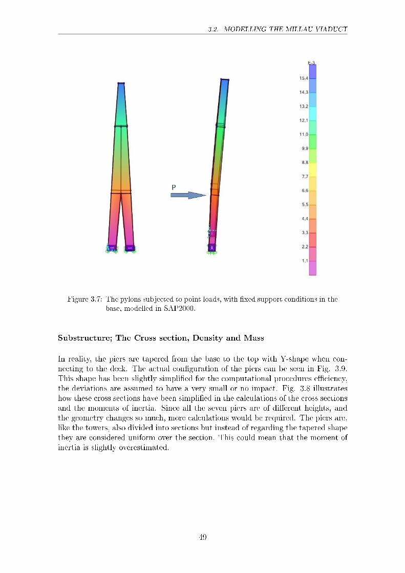
3.2. MODELLING THE MILLAU VIADUCT
Figure 3.7: The pylons subjected to point loads, with �xed support conditions in thebase, modelled in SAP2000.
Substructure; The Cross section, Density and Mass
In reality, the piers are tapered from the base to the top with Y-shape when con-necting to the deck. The actual con�guration of the piers can be seen in Fig. 3.9.This shape has been slightly simpli�ed for the computational procedures e�ciency,the deviations are assumed to have a very small or no impact. Fig. 3.8 illustrateshow these cross sections have been simpli�ed in the calculations of the cross sectionsand the moments of inertia. Since all the seven piers are of di�erent heights, andthe geometry changes so much, more calculations would be required. The piers are,like the towers, also divided into sections but instead of regarding the tapered shapethey are considered uniform over the section. This could mean that the moment ofinertia is slightly overestimated.
49
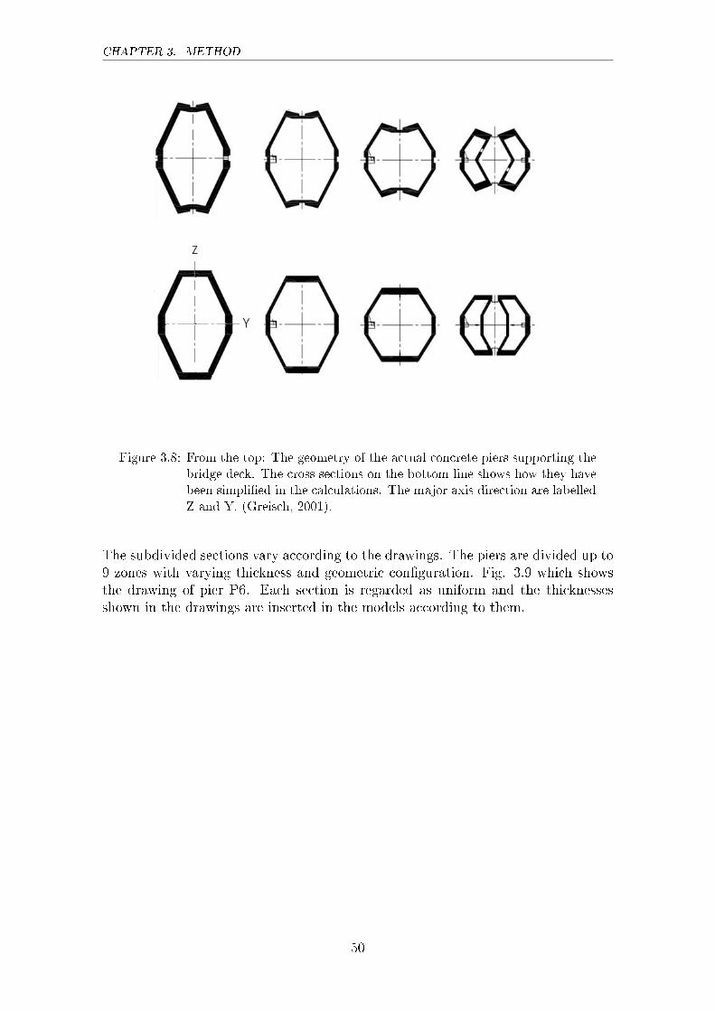
CHAPTER 3. METHOD
Figure 3.8: From the top: The geometry of the actual concrete piers supporting thebridge deck. The cross sections on the bottom line shows how they havebeen simpli�ed in the calculations. The major axis direction are labelledZ and Y. (Greisch, 2001).
The subdivided sections vary according to the drawings. The piers are divided up to9 zones with varying thickness and geometric con�guration. Fig. 3.9 which showsthe drawing of pier P6. Each section is regarded as uniform and the thicknessesshown in the drawings are inserted in the models according to them.
50
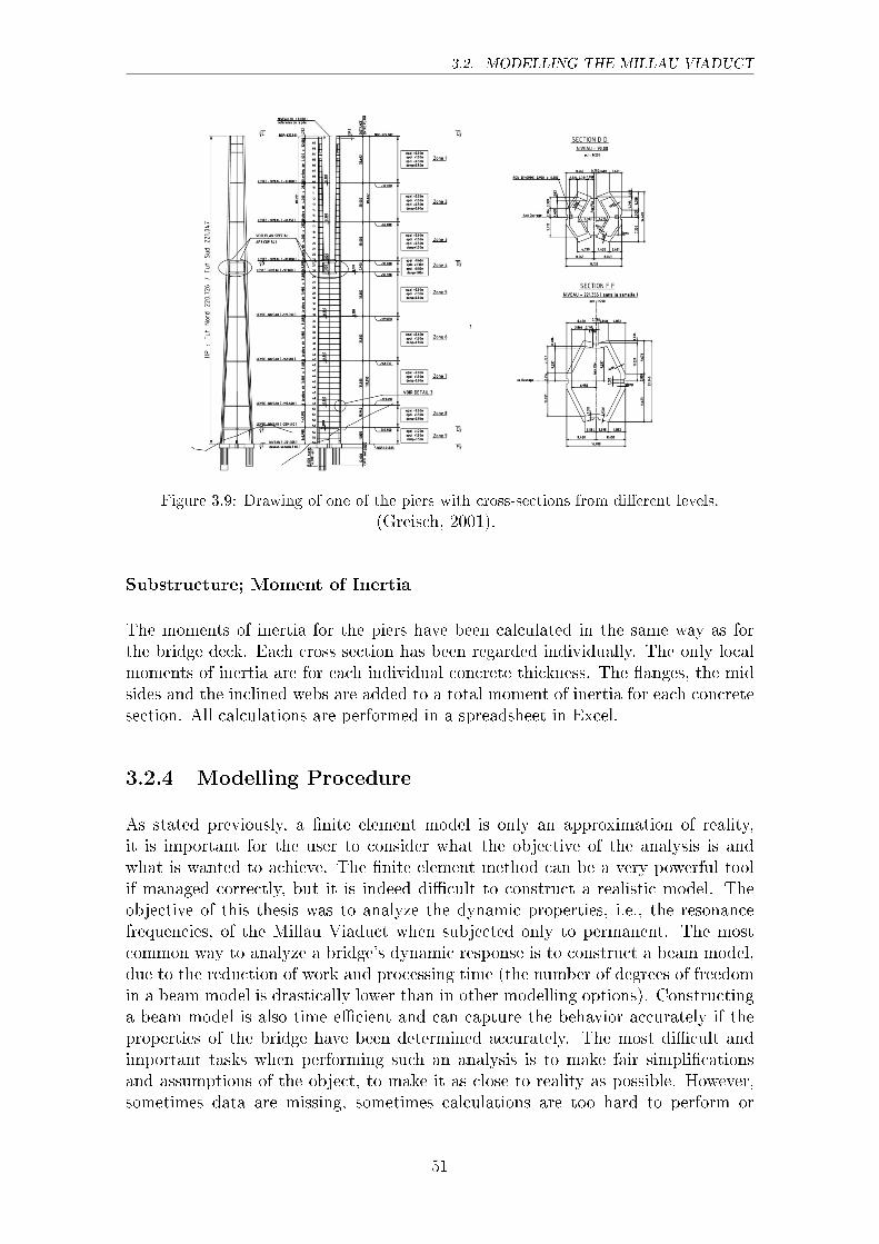
3.2. MODELLING THE MILLAU VIADUCT
Figure 3.9: Drawing of one of the piers with cross-sections from di�erent levels.
(Greisch, 2001).
Substructure; Moment of Inertia
The moments of inertia for the piers have been calculated in the same way as forthe bridge deck. Each cross section has been regarded individually. The only localmoments of inertia are for each individual concrete thickness. The �anges, the midsides and the inclined webs are added to a total moment of inertia for each concretesection. All calculations are performed in a spreadsheet in Excel.
3.2.4 Modelling Procedure
As stated previously, a �nite element model is only an approximation of reality,it is important for the user to consider what the objective of the analysis is andwhat is wanted to achieve. The �nite element method can be a very powerful toolif managed correctly, but it is indeed di�cult to construct a realistic model. Theobjective of this thesis was to analyze the dynamic properties, i.e., the resonancefrequencies, of the Millau Viaduct when subjected only to permanent. The mostcommon way to analyze a bridge's dynamic response is to construct a beam model,due to the reduction of work and processing time (the number of degrees of freedomin a beam model is drastically lower than in other modelling options). Constructinga beam model is also time e�cient and can capture the behavior accurately if theproperties of the bridge have been determined accurately. The most di�cult andimportant tasks when performing such an analysis is to make fair simpli�cationsand assumptions of the object, to make it as close to reality as possible. However,sometimes data are missing, sometimes calculations are too hard to perform or
51
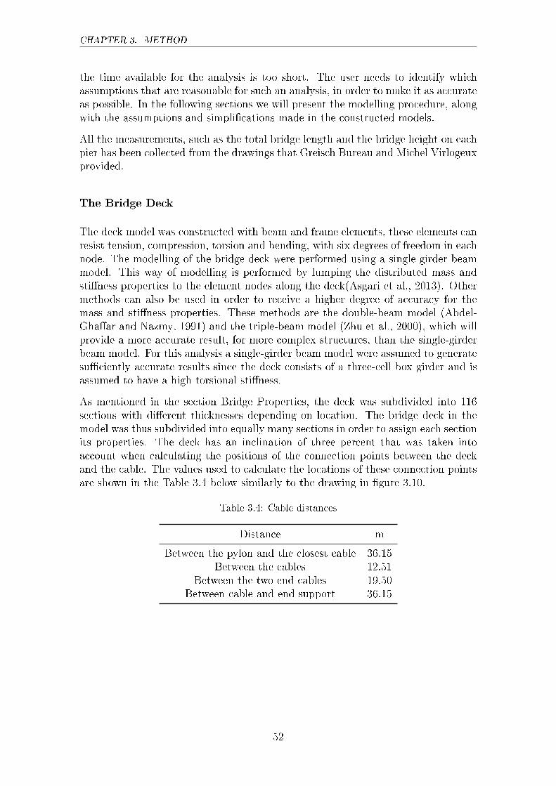
CHAPTER 3. METHOD
the time available for the analysis is too short. The user needs to identify whichassumptions that are reasonable for such an analysis, in order to make it as accurateas possible. In the following sections we will present the modelling procedure, alongwith the assumptions and simpli�cations made in the constructed models.
All the measurements, such as the total bridge length and the bridge height on eachpier has been collected from the drawings that Greisch Bureau and Michel Virlogeuxprovided.
The Bridge Deck
The deck model was constructed with beam and frame elements, these elements canresist tension, compression, torsion and bending, with six degrees of freedom in eachnode. The modelling of the bridge deck were performed using a single-girder beammodel. This way of modelling is performed by lumping the distributed mass andsti�ness properties to the element nodes along the deck(Asgari et al., 2013). Othermethods can also be used in order to receive a higher degree of accuracy for themass and sti�ness properties. These methods are the double-beam model (Abdel-Gha�ar and Nazmy, 1991) and the triple-beam model (Zhu et al., 2000), which willprovide a more accurate result, for more complex structures, than the single-girderbeam model. For this analysis a single-girder beam model were assumed to generatesu�ciently accurate results since the deck consists of a three-cell box girder and isassumed to have a high torsional sti�ness.
As mentioned in the section Bridge Properties, the deck was subdivided into 116sections with di�erent thicknesses depending on location. The bridge deck in themodel was thus subdivided into equally many sections in order to assign each sectionits properties. The deck has an inclination of three percent that was taken intoaccount when calculating the positions of the connection points between the deckand the cable. The values used to calculate the locations of these connection pointsare shown in the Table 3.4 below similarly to the drawing in �gure 3.10.
Table 3.4: Cable distances
Distance m
Between the pylon and the closest cable 36.15Between the cables 12.51
Between the two end cables 19.50Between cable and end support 36.15
52
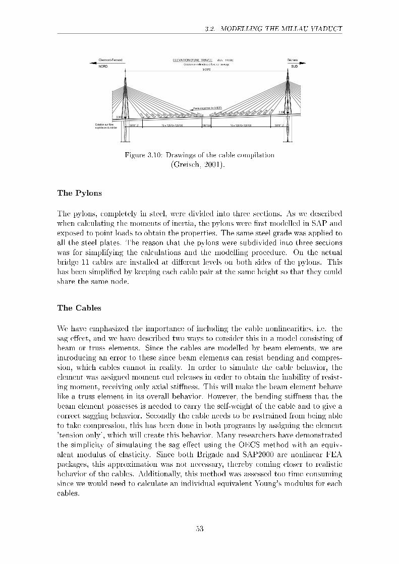
3.2. MODELLING THE MILLAU VIADUCT
Figure 3.10: Drawings of the cable compilation
(Greisch, 2001).
The Pylons
The pylons, completely in steel, were divided into three sections. As we describedwhen calculating the moments of inertia, the pylons were �rst modelled in SAP andexposed to point loads to obtain the properties. The same steel grade was applied toall the steel plates. The reason that the pylons were subdivided into three sectionswas for simplifying the calculations and the modelling procedure. On the actualbridge 11 cables are installed at di�erent levels on both sides of the pylons. Thishas been simpli�ed by keeping each cable pair at the same height so that they couldshare the same node.
The Cables
We have emphasized the importance of including the cable nonlinearities, i.e. thesag e�ect, and we have described two ways to consider this in a model consisting ofbeam or truss elements. Since the cables are modelled by beam elements, we areintroducing an error to these since beam elements can resist bending and compres-sion, which cables cannot in reality. In order to simulate the cable behavior, theelement was assigned moment end releases in order to obtain the inability of resist-ing moment, receiving only axial sti�ness. This will make the beam element behavelike a truss element in its overall behavior. However, the bending sti�ness that thebeam element possesses is needed to carry the self-weight of the cable and to give acorrect sagging behavior. Secondly the cable needs to be restrained from being ableto take compression, this has been done in both programs by assigning the element'tension only', which will create this behavior. Many researchers have demonstratedthe simplicity of simulating the sag e�ect using the OECS method with an equiv-alent modulus of elasticity. Since both Brigade and SAP2000 are nonlinear FEApackages, this approximation was not necessary, thereby coming closer to realisticbehavior of the cables. Additionally, this method was assessed too time consumingsince we would need to calculate an individual equivalent Young's modulus for eachcables.
53
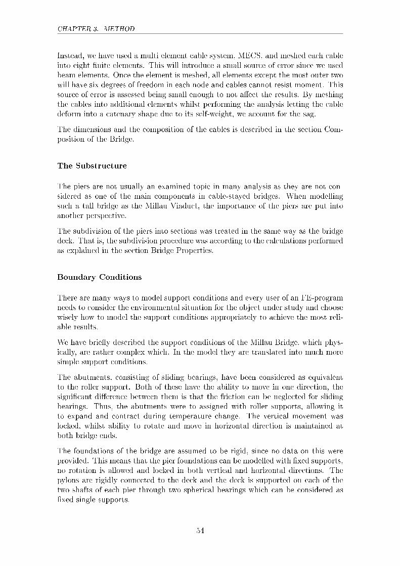
CHAPTER 3. METHOD
Instead, we have used a multi element cable system, MECS, and meshed each cableinto eight �nite elements. This will introduce a small source of error since we usedbeam elements. Once the element is meshed, all elements except the most outer twowill have six degrees of freedom in each node and cables cannot resist moment. Thissource of error is assessed being small enough to not a�ect the results. By meshingthe cables into additional elements whilst performing the analysis letting the cabledeform into a catenary shape due to its self-weight, we account for the sag.
The dimensions and the composition of the cables is described in the section Com-position of the Bridge.
The Substructure
The piers are not usually an examined topic in many analysis as they are not con-sidered as one of the main components in cable-stayed bridges. When modellingsuch a tall bridge as the Millau Viaduct, the importance of the piers are put intoanother perspective.
The subdivision of the piers into sections was treated in the same way as the bridgedeck. That is, the subdivision procedure was according to the calculations performedas explained in the section Bridge Properties.
Boundary Conditions
There are many ways to model support conditions and every user of an FE-programneeds to consider the environmental situation for the object under study and choosewisely how to model the support conditions appropriately to achieve the most reli-able results.
We have brie�y described the support conditions of the Millau Bridge, which phys-ically, are rather complex which. In the model they are translated into much moresimple support conditions.
The abutments, consisting of sliding bearings, have been considered as equivalentto the roller support. Both of these have the ability to move in one direction, thesigni�cant di�erence between them is that the friction can be neglected for slidingbearings. Thus, the abutments were to assigned with roller supports, allowing itto expand and contract during temperature change. The vertical movement waslocked, whilst ability to rotate and move in horizontal direction is maintained atboth bridge ends.
The foundations of the bridge are assumed to be rigid, since no data on this wereprovided. This means that the pier foundations can be modelled with �xed supports,no rotation is allowed and locked in both vertical and horizontal directions. Thepylons are rigidly connected to the deck and the deck is supported on each of thetwo shafts of each pier through two spherical bearings which can be considered as�xed single supports.
54
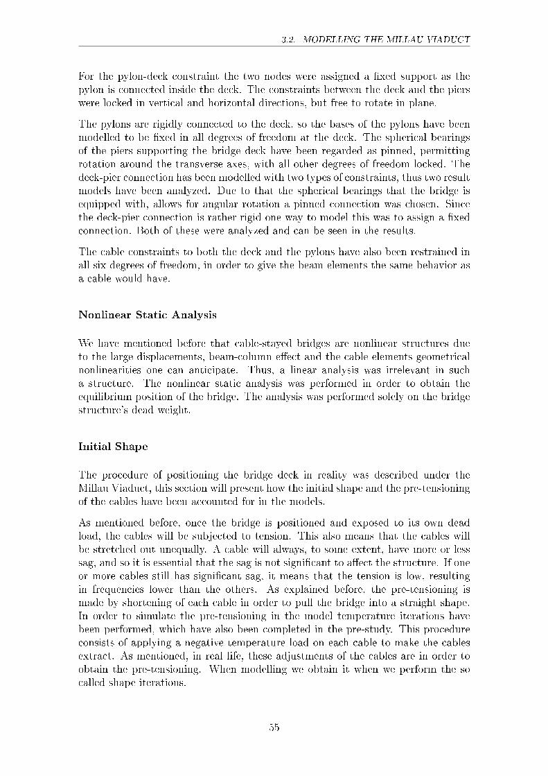
3.2. MODELLING THE MILLAU VIADUCT
For the pylon-deck constraint the two nodes were assigned a �xed support as thepylon is connected inside the deck. The constraints between the deck and the pierswere locked in vertical and horizontal directions, but free to rotate in plane.
The pylons are rigidly connected to the deck, so the bases of the pylons have beenmodelled to be �xed in all degrees of freedom at the deck. The spherical bearingsof the piers supporting the bridge deck have been regarded as pinned, permittingrotation around the transverse axes, with all other degrees of freedom locked. Thedeck-pier connection has been modelled with two types of constraints, thus two resultmodels have been analyzed. Due to that the spherical bearings that the bridge isequipped with, allows for angular rotation a pinned connection was chosen. Sincethe deck-pier connection is rather rigid one way to model this was to assign a �xedconnection. Both of these were analyzed and can be seen in the results.
The cable constraints to both the deck and the pylons have also been restrained inall six degrees of freedom, in order to give the beam elements the same behavior asa cable would have.
Nonlinear Static Analysis
We have mentioned before that cable-stayed bridges are nonlinear structures dueto the large displacements, beam-column e�ect and the cable elements geometricalnonlinearities one can anticipate. Thus, a linear analysis was irrelevant in sucha structure. The nonlinear static analysis was performed in order to obtain theequilibrium position of the bridge. The analysis was performed solely on the bridgestructure's dead weight.
Initial Shape
The procedure of positioning the bridge deck in reality was described under theMillau Viaduct, this section will present how the initial shape and the pre-tensioningof the cables have been accounted for in the models.
As mentioned before, once the bridge is positioned and exposed to its own deadload, the cables will be subjected to tension. This also means that the cables willbe stretched out unequally. A cable will always, to some extent, have more or lesssag, and so it is essential that the sag is not signi�cant to a�ect the structure. If oneor more cables still has signi�cant sag, it means that the tension is low, resultingin frequencies lower than the others. As explained before, the pre-tensioning ismade by shortening of each cable in order to pull the bridge into a straight shape.In order to simulate the pre-tensioning in the model temperature iterations havebeen performed, which have also been completed in the pre-study. This procedureconsists of applying a negative temperature load on each cable to make the cablesextract. As mentioned, in real life, these adjustments of the cables are in order toobtain the pre-tensioning. When modelling we obtain it when we perform the socalled shape iterations.
55
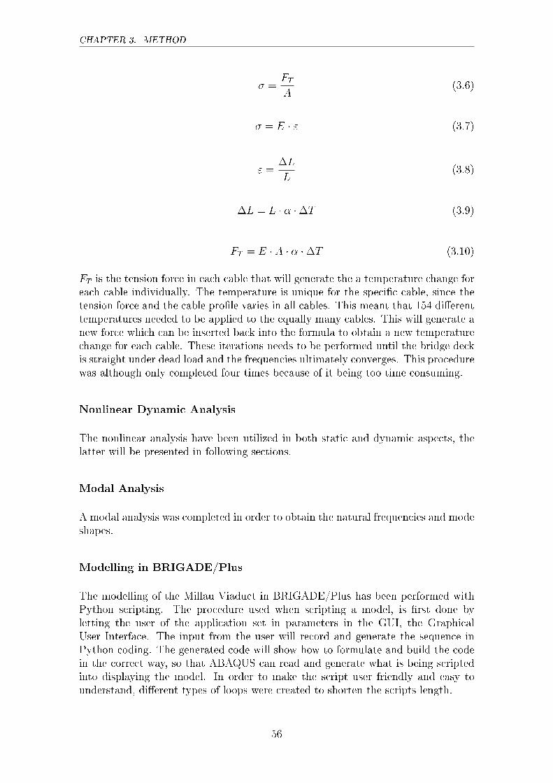
CHAPTER 3. METHOD
� =FT
A(3.6)
� = E � " (3.7)
" =�L
L(3.8)
�L = L � � ��T (3.9)
FT = E � A � � ��T (3.10)
FT is the tension force in each cable that will generate the a temperature change foreach cable individually. The temperature is unique for the speci�c cable, since thetension force and the cable pro�le varies in all cables. This meant that 154 di�erenttemperatures needed to be applied to the equally many cables. This will generate anew force which can be inserted back into the formula to obtain a new temperaturechange for each cable. These iterations needs to be performed until the bridge deckis straight under dead load and the frequencies ultimately converges. This procedurewas although only completed four times because of it being too time consuming.
Nonlinear Dynamic Analysis
The nonlinear analysis have been utilized in both static and dynamic aspects, thelatter will be presented in following sections.
Modal Analysis
A modal analysis was completed in order to obtain the natural frequencies and modeshapes.
Modelling in BRIGADE/Plus
The modelling of the Millau Viaduct in BRIGADE/Plus has been performed withPython scripting. The procedure used when scripting a model, is �rst done byletting the user of the application set in parameters in the GUI, the GraphicalUser Interface. The input from the user will record and generate the sequence inPython coding. The generated code will show how to formulate and build the codein the correct way, so that ABAQUS can read and generate what is being scriptedinto displaying the model. In order to make the script user friendly and easy tounderstand, di�erent types of loops were created to shorten the scripts length.
56
3.2. MODELLING THE MILLAU VIADUCT
The script is built in a manner that it's calculating the coordinates of each nodeneeded to construct the model. These coordinates are then called upon as attributesto functions, whose task is to perform one prede�ned operation. The function usedin this script has been programmed to construct lines, assign attributes, import dataand then return these values to build the model.
A good way to keep track of important nodes or elements is to create a set out ofthem. A set allows you to call this certain node or element that has been createdto be used in other purposes, for example assign them a cross-section or addingboundary conditions to that speci�c part. They can also be used for extractingdata, when the analysis has been performed, then the data can be extracted andread for further analysis.
BRIGADE/Plus is divided into a number of modules in which the modelling proce-dure will be described in the following sections
Part A tall cable-stayed bridge consists of four major parts and so does this script,it contain deck, pylons, cables and substructure. The di�erent parts were createdusing deformable wires. Since the moment of inertia is changing in the di�erentparts, coordinates were calculated to create elements of the same moment of inertia.These coordinates were then called as attributes to the functions for each part. Insidethe function for-loops were used to draw the lines representing the part. Each partwill then be able to have sets connected to them and so be easier to work with.
Property The di�erent parts were assigned material properties. The cables weregiven a circular pro�le but for all the other parts a general pro�le had to be created.The data needed for the bridge component's properties were imported from Exceland assigned each pro�le. Each pro�le was connected to a speci�c set, representingthe element that was to be given the attributes. A beam orientation was made foreach part to de�ne the local major axis of the cross-section.
Assembly When a part is created, it is independent of any other parts constructedin the model, and exists only in its own coordinate system. Instances are createdto represent that part, in the global coordinate system called the Assembly. Herethe instances of each part will be positioned with the other parts. These instancescan then be copied and moved, to generate the assembled model. Each assembly isconnected to the part, meaning that you cannot have di�erent values on di�erentinstances of the same part.
The pylons and the cables were given di�erent dimension so more then one objecthad to be created in the part. The pylon part consisted of seven pylons with threedi�erent section, created as one instance. Likewise the cable part was created withseven cable pairs each consisted of 22 cables as one instance. All seven substructureswith di�erent length were also created as one instance and so also the deck.
As can be seen above a model can consist of many parts and even more instances,
57
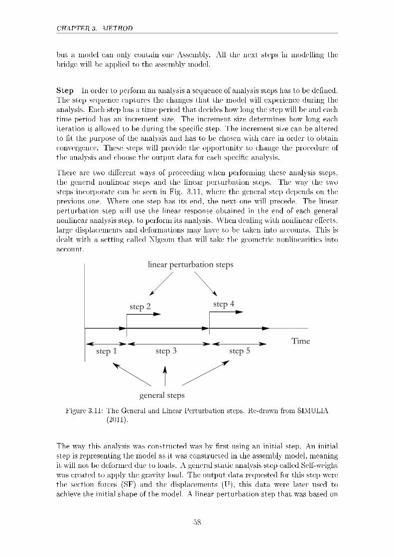
CHAPTER 3. METHOD
but a model can only contain one Assembly. All the next steps in modelling thebridge will be applied to the assembly model.
Step In order to perform an analysis a sequence of analysis steps has to be de�ned.The step sequence captures the changes that the model will experience during theanalysis. Each step has a time period that decides how long the step will be and eachtime period has an increment size. The increment size determines how long eachiteration is allowed to be during the speci�c step. The increment size can be alteredto �t the purpose of the analysis and has to be chosen with care in order to obtainconvergence. These steps will provide the opportunity to change the procedure ofthe analysis and choose the output data for each speci�c analysis.
There are two di�erent ways of proceeding when performing these analysis steps,the general nonlinear steps and the linear perturbation steps. The way the twosteps incorporate can be seen in Fig. 3.11, where the general step depends on theprevious one. Where one step has its end, the next one will precede. The linearperturbation step will use the linear response obtained in the end of each generalnonlinear analysis step, to perform its analysis. When dealing with nonlinear e�ects,large displacements and deformations may have to be taken into accounts. This isdealt with a setting called Nlgeom that will take the geometric nonlinearities intoaccount.
linear perturbation steps
step 2 step 4
step 3step 1 step 5Time
general steps
Figure 3.11: The General and Linear Perturbation steps. Re-drawn from SIMULIA(2011).
The way this analysis was constructed was by �rst using an initial step. An initialstep is representing the model as it was constructed in the assembly model, meaningit will not be deformed due to loads. A general static analysis step called Self-weightwas created to apply the gravity load. The output data requested for this step werethe section forces (SF) and the displacements (U), this data were later used toachieve the initial shape of the model. A linear perturbation step that was based on
58
3.2. MODELLING THE MILLAU VIADUCT
the Self-weight step, was constructed as a Frequency step. In order to obtain modeshapes and to calculate the natural frequencies an eigenvalue extraction procedurehad to be chosen. There are three di�erent extraction methods in BRIGADE/Plus;the Lanczos, the AMS (Automatic multi-level substructuring) and the Subspacemethod. The method that was used in performing the analysis was the Subspacemethod, since it is easy to use and better suited for complex eigenvalue problems.
Interaction The assembled model consists of instances that are located in thesame space but they are not connected with each other, even if they share the samecoordinate. Constraints have to be assigned the instances in order for them to beconnected. There are many di�erent types of constraints, used for di�erent purposes,for more information on what constraint to use see the ABAQUS manual.
One and the same constraint was used for all the di�erent interaction points, thiswas the coupling constraint. The purpose of a coupling constraint is to constrainthe motion of a surface to the motion of a single point. There are two di�erentways to construct this constraint, the kinematic or distributing constraint type.The kinematic coupling constraint was the one chosen since it allows the user tocontrol both the translational and the rotational degrees of freedom at the couplingnode. In all connections the translational degrees of freedom were locked, makingthe coupling node follow the motion of the reference node. Two models were madeone with all the rotational degrees of freedom locked for the connection betweendeck and substructure and one that allowed for rotation of the deck around thetransversal axis. All other coupling nodes had the rotational degrees of freedomlocked.
When constructing couple constraints, the surface node cannot be controlled by twodi�erent reference nodes, but a reference node can control two surfaces. Even thoughtwo cables shared the same coordinate at each pylon, two coupling nodes had to beassigned with the pylon to act as the reference node. This allowed the cables tomove as two separate cables. If only one coupling was to be made, the cables wouldhave moved in symbiosis with a constant angle between them in the analysis. Thepylons were set to follow the motion of the deck and so was also the substructure.
Load Loads and boundary conditions were speci�ed. The boundary conditionswere as described above, and the gravity load was set to be uniformly distributedover the whole model. Since a pre-tensioning force was to be introduced to thecables, temperature loads were created in the prede�ned �eld, one for each cable.
Mesh In order to receive more accurate results, the model was divided into smallerelements. There are di�erent ways of meshing an object, as previously described inthe BRIGADE chapter.
The tool seed edges was used to perform the mesh. This tool allows for both choosingthe number of sub-division of each element and also the size of each element. Localseeds were then distributed over the model to decide the density of the mesh over
59
CHAPTER 3. METHOD
the instances. The cables were given an equal number of elements, and the numberof elements were eight. The seeds were then placed at an interval of maximum �vemeters for each element, this was believed to give an accurate enough result seen tothe time it took to compute.
Job When creating an analysis BRIGADE/Plus creates a job, containing the as-sembled model with the analysis steps de�ned in the step module. The results areshown in the Visualization module.
Visualization The results of the analysis and also the �nite element model aredisplayed in the Visualization module. The results from the de�ned steps, at di�er-ent time increments are shown for the self-weight step and also di�erent frequenciesat these time steps. The results are printed into text �les, called dat and msg �les.
Shape iteration When the analysis were done and results provided a new scriptwas initiated. This script gathered the results that were previously requested in theoutput data. In order to receive these data, a reference node had to be created wherethe displacements were to be collected. These nodes were located at the end of eachcable, connected to the deck. The section forces works along the entire element,and since the cable consisted of eight elements, eight di�erent section forces wereobtained. Since each cable was to be given one temperature change along the entirecable, the last element connected to the deck, was chosen to re�ect the section forceworking along the entire cable. The data extracted from the cables were then usedin �nding the initial shape of the model.
Modelling in SAP2000
The model is solely in frame elements,which is the simplest element to use whenmodelling in SAP. This was very practical since Brigade has the equivalent beamelement.
Building the model Contrary to how BRIGADE has been managed, SAP2000has been managed directly in the GUI. In SAP all components can be modelledat the same time in the same window and will still be created as one part each.The model can �rst be built using a standard element of choice or the user mayde�ne the elements with the desired properties by �rst de�ning each element thatare to build the model. It really doesn't matter which method is chosen, as long asthe user keeps track of the procedure. Since we wanted to build a model entirely inframe elements, the simplest working process was to build the model with the correctgeometry and afterwards creating the properties for each part. The whole bridge wasthus created as one whole part in the same standard frame element, in SAP titledFSEC1. By assigning the di�erent components their correct structural parameteri.e. cross sectional and material, the user will disassemble the model into groups of
60
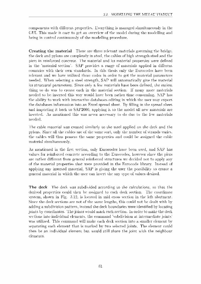
3.2. MODELLING THE MILLAU VIADUCT
components with di�erent properties. Everything is managed simultaneously in theGUI. This made it easy to get an overview of the model during the modelling andbeing in control continuously of the modelling procedure.
Creating the material There are three relevant materials governing the bridge,the deck and pylons are completely in steel, the cables of high strength steel and thepiers in reinforced concrete. The material and its material properties were de�nedin the 'material section'. SAP provides a range of materials applied in di�erentcountries with their own standards. In this thesis only the Eurocodes have beenrelevant and we have utilized these codes in order to get the material parametersneeded. When selecting a steel strength, SAP will automatically give the materialits structural parameters. Since only a few materials have been de�ned, the easiestthing to do was to create each in the material section. If many more materialsneeded to be inserted this way would have been rather time consuming. SAP hasthe ability to work with interactive databases editing in which the user may exportthe databases information into an Excel spread sheet. By �lling in the spread sheetand importing it back to SAP2000, applying it to the model all new materials areinserted. As mentioned this was never necessary to do due to the few materialsneeded.
The cable material was created similarly to the steel applied on the deck and thepylons. Since all the cables are of the same sort, only the number of strands varies,the cables will thus possess the same properties and could be assigned the cablematerial simultaneously.
As mentioned in the �rst section, only Eurocodes have been used, and SAP hasvalues for reinforced concrete according to the Eurocodes, however since the piersare rather di�erent from general reinforced structures we decided not to apply anyof the material properties that were provided in the Eurocode library. Instead ofapplying any inserted material, SAP is giving the user the possibility to create ageneral material in which the user can insert the any type of values desired.
The deck The deck was subdivided according to the calculations, so that thederived properties could then be assigned to each deck section. The coordinatesystem, shown in Fig. 3.12, is located in mid cross section in the left abutment.Since the deck sections are not of the same lengths, this could not be dealt with byadding a subdivision pattern, instead the deck boundaries were identi�ed by locatingjoints by coordinates. The joints would mark each section. In order to make the decksections into individual elements, the command 'subdivision at intermediate joints'was utilized. This command will make each deck section into a smaller element byseparating each element that is marked by two selected joints. The element couldthen be an individual element but would still share the joint with the neighbourelements.
61
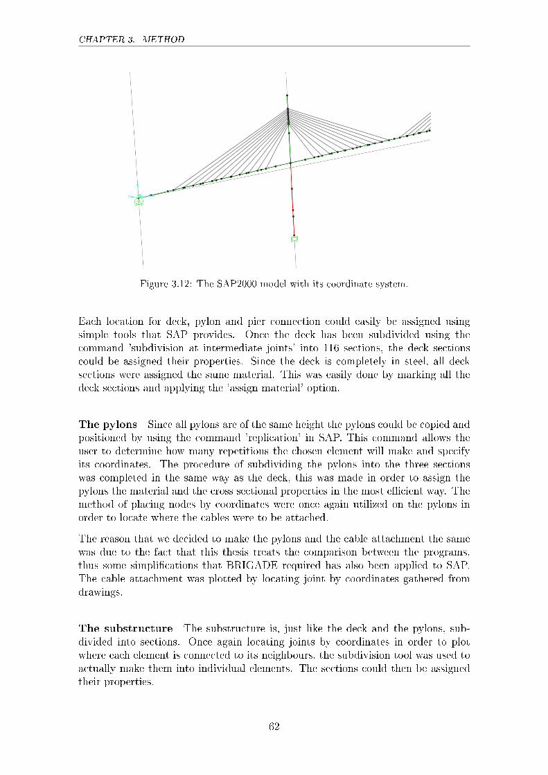
CHAPTER 3. METHOD
Figure 3.12: The SAP2000 model with its coordinate system.
Each location for deck, pylon and pier connection could easily be assigned usingsimple tools that SAP provides. Once the deck has been subdivided using thecommand 'subdivision at intermediate joints' into 116 sections, the deck sectionscould be assigned their properties. Since the deck is completely in steel, all decksections were assigned the same material. This was easily done by marking all thedeck sections and applying the 'assign material' option.
The pylons Since all pylons are of the same height the pylons could be copied andpositioned by using the command 'replication' in SAP. This command allows theuser to determine how many repetitions the chosen element will make and specifyits coordinates. The procedure of subdividing the pylons into the three sectionswas completed in the same way as the deck, this was made in order to assign thepylons the material and the cross sectional properties in the most e�cient way. Themethod of placing nodes by coordinates were once again utilized on the pylons inorder to locate where the cables were to be attached.
The reason that we decided to make the pylons and the cable attachment the samewas due to the fact that this thesis treats the comparison between the programs,thus some simpli�cations that BRIGADE required has also been applied to SAP.The cable attachment was plotted by locating joint by coordinates gathered fromdrawings.
The substructure The substructure is, just like the deck and the pylons, sub-divided into sections. Once again locating joints by coordinates in order to plotwhere each element is connected to its neighbours, the subdivision tool was used toactually make them into individual elements. The sections could then be assignedtheir properties.
62
3.2. MODELLING THE MILLAU VIADUCT
Assigning the properties to the beam model After the model was completedand the subdivision, distinguishing each component, had been made each of theelements were to be assigned the properties. First of all, the properties along witha general element for each section had to be created and inserted into SAP.
Fortunately, this did not need to be done manually, like mentioned in the section'Creating the Material', SAP operates with Excel by using interactive databaseswhich makes it much more time e�cient. In the Edit menu, the user can open theinteractive databases menu where all information about the model is available. Theability to insert speci�c desired values like density, masses, cross sectional propertiesetc is available. This option becomes very handy when many values needs to beinserted. This option made the modelling procedure much quicker than if insertingeach property manually.
The Excel spreadsheet was very much appreciated since all calculations performedwere completed in Excel and could thus be easily collected and inserted into theSAP2000 spread sheet. All of the sections except for the cables were created asgeneral sections. Since we have basically lumped all properties into beam elements,the elements will naturally not have a speci�c cross section. The moments of in-ertia, cross section area and the torsional constant were inserted along with thespeci�ed element. However, when it was necessary to use the Excel spreadsheetto import properties, all sorts of structural properties such as shear area, sectionmodulus, plastic modulus, shear center etc. could have been de�ned. These havebeen neglected in SAP and will thus not be accounted for. These were not neededfor any of the programs to complete the analysis. The cables were inserted one byone by the command 'De�ne Element'. By inserting the cable area manually, SAPautomatically calculates the structural parameters of the element.
Boundary conditions and constraints To determine where the bridge deckmeets the pier and the pylon, every joint for each of the seven deck-pier-pylonconnections where placed by coordinates, this would then result in all of them sharingthat very joint. This would make the connection become rigid. In order to get thestructural mechanics correct, the deck must be continuous along its length, and beable to control the support conditions between deck-pylon and deck-pier individually.Thus, the joint connecting all the components was disconnected resulting in fourindividual joints, the end joint of the deck element to the left of the pylon, the startjoint of the deck element on the other side of the pylon, the joint at the top of thepier and the joint at the bottom of the pylon. Once the joint is disconnected onecan start merging the appropriate joints that will create the desired behavior.
Two methods were tested in order to see which of the methods that would be mostappropriate for the support conditions.
Method 1. Creating two constraints A constraint in SAP2000 is a set of two ormore joints that are constrained such that their displacements relate (CSIAmerica,2015). Constraints may be used to model rigid-body behavior, in which joints
63
CHAPTER 3. METHOD
translate and rotate together in a rigid connection; equal-displacement behavior,in which displacements along certain degrees of freedom, is equal; and symmetry /anti-symmetry conditions (CSIAmerica, 2015). Constraints enhance computationale�ciency by reducing the number of equations necessary for solution.
To create these constraints either body constraints or weld constraints may be uti-lized, in our case the latter became relevant. Body constraints are explained by CSIAmerica as 'A Body constraint is applied to a set of joints that translate and ro-tate together as a rigid body. Rigid behavior is automatically applied to all degreesof freedom within the constraint, though only certain degrees of freedom may bespeci�ed' (CSIAmerica, 2015).
Weld constraints operates in the same way as body constraints, the di�erence isthat only these constraints connects joints within a small tolerance. This meansthat if the same constraints are needed in multiple locations in the same model, theweld constraints are practical since it only operates with joints in the same area.The problem with Body constraints is that when applying the same constraint inseveral places in the model, all of the joints will try to connect with each other whichwill make the behavior erroneous. This was tested in the SAP2000 model in thebeginning at �rst which ultimately gave rise to errors. Since the support conditionsbetween the pylon and deck, deck and pier are of the same character for all sevenpiers and towers, the same body constraint were assigned to them all which made thejoints trying to achieve a connection with each other causing all the pier-deck-pylonto move in one unit.
Body constraints are not really wrong to use, but an individual constraint for eachlocation must be created in order to be applied only in the assigned area. However,creating the same body constraint for a new area seemed rather time consuming andunnecessary. If anything needs to be changed then it needs to be changed in all thecreated constraints. When using weld constraints only one constraint would needto be de�ned, since it would only connect to joints within a certain tolerance. Anyspeci�c changes needed, could therefore be easily changed once. Thus the decisionusing weld constraints were ultimately the choice.
After disconnecting the joint connection between the deck, pylon and pier, therewere four individual joints; two deck joints, the joint in the bottom of the pylonand the top of the pier. The two resulting deck joints were connected by merginginto one joint, making the deck continuous. In order to get the presuppositionsfor the support conditions for the joints deck-pylon and pier-deck, we created twoconstraints in which the connection between the deck and the pylon are based onterms that the connection is completely �xed. The connection between the deckand the pier is considered as pinned. The constraints are created by allowing norotation or translations whatsoever between the deck and the pylon, whereas onlyrotation around the Y-axis, is allowed between the deck and the pier.
By selecting the deck joint and the pylon joint simultaneously we could assign theconstraints between them. This procedure is shown in �gure (3.13)
64
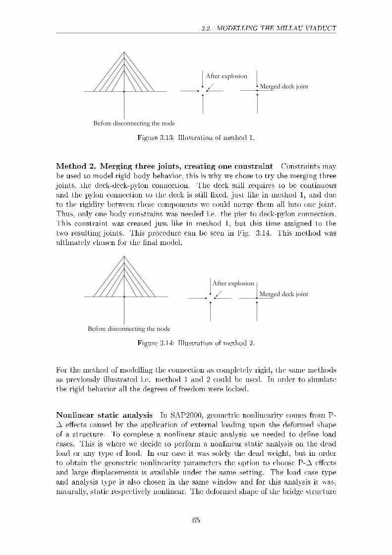
3.2. MODELLING THE MILLAU VIADUCT
After explosion
Merged deck joint
Before disconnecting the node
Figure 3.13: Illustration of method 1.
Method 2. Merging three joints, creating one constraint Constraints maybe used to model rigid-body behavior, this is why we chose to try the merging threejoints, the deck-deck-pylon connection. The deck still requires to be continuousand the pylon connection to the deck is still �xed, just like in method 1, and dueto the rigidity between these components we could merge them all into one joint.Thus, only one body constraint was needed i.e. the pier to deck-pylon connection.This constraint was created just like in method 1, but this time assigned to thetwo resulting joints. This procedure can be seen in Fig. 3.14. This method wasultimately chosen for the �nal model.
After explosion
Merged deck joint
Before disconnecting the node
Figure 3.14: Illustration of method 2.
For the method of modelling the connection as completely rigid, the same methodsas previously illustrated i.e. method 1 and 2 could be used. In order to simulatethe rigid behavior all the degrees of freedom were locked.
Nonlinear static analysis In SAP2000, geometric nonlinearity comes from P-� e�ects caused by the application of external loading upon the deformed shapeof a structure. To complete a nonlinear static analysis we needed to de�ne loadcases. This is where we decide to perform a nonlinear static analysis on the deadload or any type of load. In our case it was solely the dead weight, but in orderto obtain the geometric nonlinearity parameters the option to choose P-� e�ectsand large displacements is available under the same setting. The load case typeand analysis type is also chosen in the same window and for this analysis it was,naturally, static respectively nonlinear. The deformed shape of the bridge structure
65
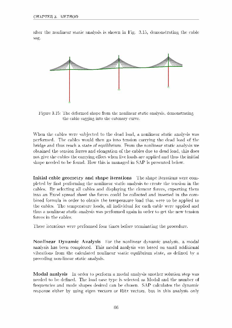
CHAPTER 3. METHOD
after the nonlinear static analysis is shown in Fig. 3.15, demonstrating the cablesag.
Figure 3.15: The deformed shape from the nonlinear static analysis, demonstratingthe cable sagging into the catenary curve.
When the cables were subjected to the dead load, a nonlinear static analysis wasperformed. The cables would then go into tension carrying the dead load of thebridge and thus reach a state of equilibrium. From the nonlinear static analysis weobtained the tension forces and elongation of the cables due to dead load, this doesnot give the cables the carrying e�ect when live loads are applied and thus the initialshape needed to be found. How this is managed in SAP is presented below.
Initial cable geometry and shape iterations The shape iterations were com-pleted by �rst performing the nonlinear static analysis to create the tension in thecables. By selecting all cables and displaying the element forces, exporting theminto an Excel spread sheet the forces could be collected and inserted in the com-bined formula in order to obtain the temperature load that were to be applied tothe cables. The temperature loads, all individual for each cable were applied andthus a nonlinear static analysis was performed again in order to get the new tensionforces in the cables.
These iterations were performed four times before terminating the procedure.
Nonlinear Dynamic Analysis For the nonlinear dynamic analysis, a modalanalysis has been completed. This modal analysis was based on small additionalvibrations from the calculated nonlinear static equlibrium state, as de�ned by apreceding non-linear static analysis.
Modal analysis In order to perform a modal analysis another solution step wasneeded to be de�ned. The load case type is selected as Modal and the number offrequencies and mode shapes desired can be chosen. SAP calculates the dynamicresponse either by using eigen vectors or Ritz vectors, but in this analysis only
66
3.3. THE ANALYZED MODELS
eigen vectors have been used. It is necessary to calculate the mode shapes basedon a stressed situation, starting from de�ning a static nonlinear load case withpermanent loads, like performed in the previous section and then make the modalanalysis start with an initial sti�ness iterated from the nonlinear static case. Thisoption, 'sti�ness at end of nonlinear case' were selected under the Modal load case.
3.3 The Analyzed Models
The two models, created in both programs, have been re�ned with more accuracystep by step to evaluate what was necessary to account for and what had less impact.The number of re�nements of the models had to be limited in order to remain withinthe time line. Both models presented in the thesis generate fair results, the mainresult is presented as the �nal model and the other as alternative result. Both arepresented in the result chapter.
The models have been treated equally in both programs in order to make a faircomparison. Di�erences in how the data is being processed in the programs maya�ect the results. The algorithms that the software are based upon have not beenfurther researched, nor have we been able to examine what types of mathematicalsolution methods are utilized in the programs or how these may have an impact onthe results.
Additionally, the beam theories has not been consistent in both programs, it hasbeen applied in which it serves the best purpose. This is discussed in the chapterConcluding Remarks and Further Work.
67

Chapter 4
Results
4.1 Overview
A �nite element analysis has been conducted to compare the dynamic responsesof the Millau Viaduct. The comparison was between the two programs SAP2000and BRIGADE/Plus, measured values of the viaduct and also with the frequenciescalculated from the FE-model made by the company Greisch. These can be foundunder 'Initial' in the tables. Two types of models were made in both programs,one with �xed constraints and one with pinned constraints between the deck-pierconnections. The results are presented in this chapter, starting with the �xed con-nection. The frequencies are �rst displayed in a table followed by the �rst �ve modeshapes in the vertical and transversal direction.
We have compared our mode shapes with the measured mode shapes in reality,however the design team have compared their measured mode shapes with theirown theoretical FE-model. Thus, we cannot speci�cally say that the measured modeshapes appeared in the same order that the FE-model showed. We believe that themeasured mode shapes have been matched with the initial FE-model, hence wematched the mode shapes from the SAP and BRIGADE models with the measured.This is why some of the lower frequencies can be found in the higher modes and viceversa.
Mode number two appeared as a longitudinal in the initial model, but during themeasuring of the modes there was no wind that would give rise to longitudinal modeshapes. Thus the second mode was precluded from the SAP and BRIGADE modelsbecause there were nothing to compare.
Since �ve of the �rst transversal and vertical mode shapes are presented, modenumber 11 is not included as it is the sixth transversal mode. Number 12 is the �fthvertical mode.
69
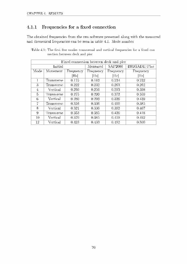
CHAPTER 4. RESULTS
4.1.1 Frequencies for a �xed connection
The obtained frequencies from the two software presented along with the measuredand theoretical frequencies can be seen in table 4.1. Mode number
Table 4.1: The �rst �ve modes transversal and vertical frequencies for a �xed con-nection between deck and pier
Fixed connection between deck and pierInitial Measured SAP2000 BRIGADE/Plus
Mode Movement Frequency Frequency Frequency Frequency[Hz] [Hz] [Hz] [Hz]
1 Transverse 0.175 0.183 0.234 0.2323 Transverse 0.222 0.232 0.263 0.2624 Vertical 0.250 0.256 0.293 0.3985 Transverse 0.275 0.299 0.372 0.3596 Vertical 0.280 0.293 0.336 0.4397 Transverse 0.316 0.336 0.400 0.3858 Vertical 0.321 0.336 0.392 0.4679 Transverse 0.353 0.385 0.436 0.41810 Vertical 0.370 0.385 0.459 0.49212 Vertical 0.423 0.433 0.492 0.500
70
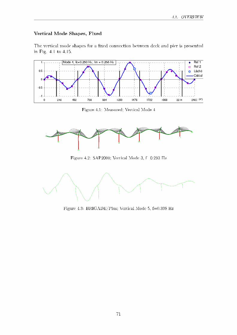
4.1. OVERVIEW
Vertical Mode Shapes, Fixed
The vertical mode shapes for a �xed connection between deck and pier is presentedin Fig. 4.1 to 4.15.
Figure 4.1: Measured; Vertical Mode 4
Figure 4.2: SAP2000; Vertical Mode 3, f=0.293 Hz
Figure 4.3: BRIGADE/Plus; Vertical Mode 5, f=0.398 Hz
71
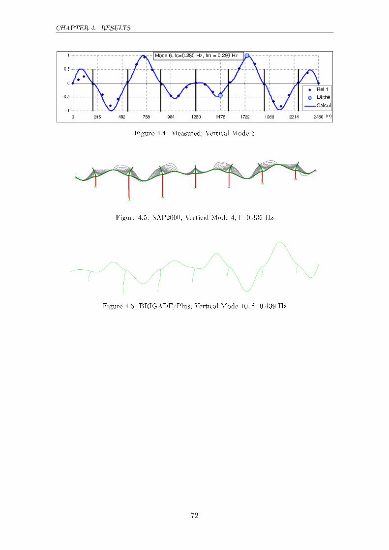
CHAPTER 4. RESULTS
Figure 4.4: Measured; Vertical Mode 6
Figure 4.5: SAP2000; Vertical Mode 4, f=0.336 Hz
Figure 4.6: BRIGADE/Plus; Vertical Mode 10, f=0.439 Hz
72
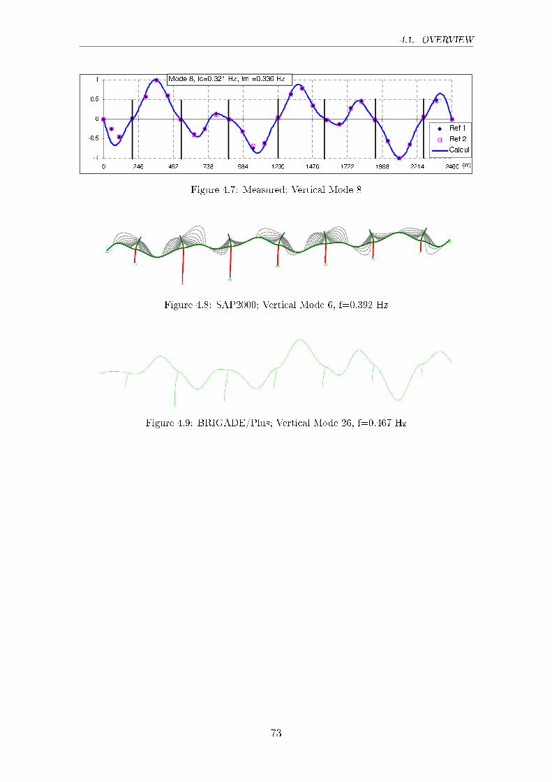
4.1. OVERVIEW
Figure 4.7: Measured; Vertical Mode 8
Figure 4.8: SAP2000; Vertical Mode 6, f=0.392 Hz
Figure 4.9: BRIGADE/Plus; Vertical Mode 26, f=0.467 Hz
73
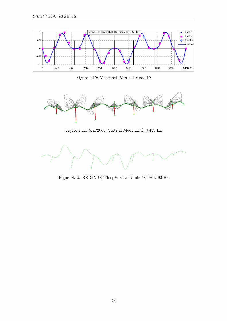
CHAPTER 4. RESULTS
Figure 4.10: Measured; Vertical Mode 10
Figure 4.11: SAP2000; Vertical Mode 11, f=0.459 Hz
Figure 4.12: BRIGADE/Plus; Vertical Mode 48, f=0.492 Hz
74
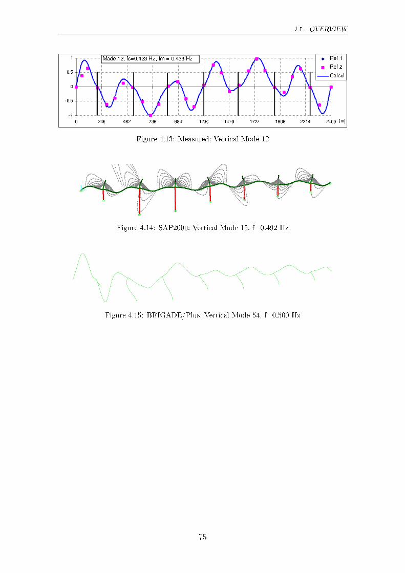
4.1. OVERVIEW
Figure 4.13: Measured; Vertical Mode 12
Figure 4.14: SAP2000; Vertical Mode 15, f=0.492 Hz
Figure 4.15: BRIGADE/Plus; Vertical Mode 54, f=0.500 Hz
75
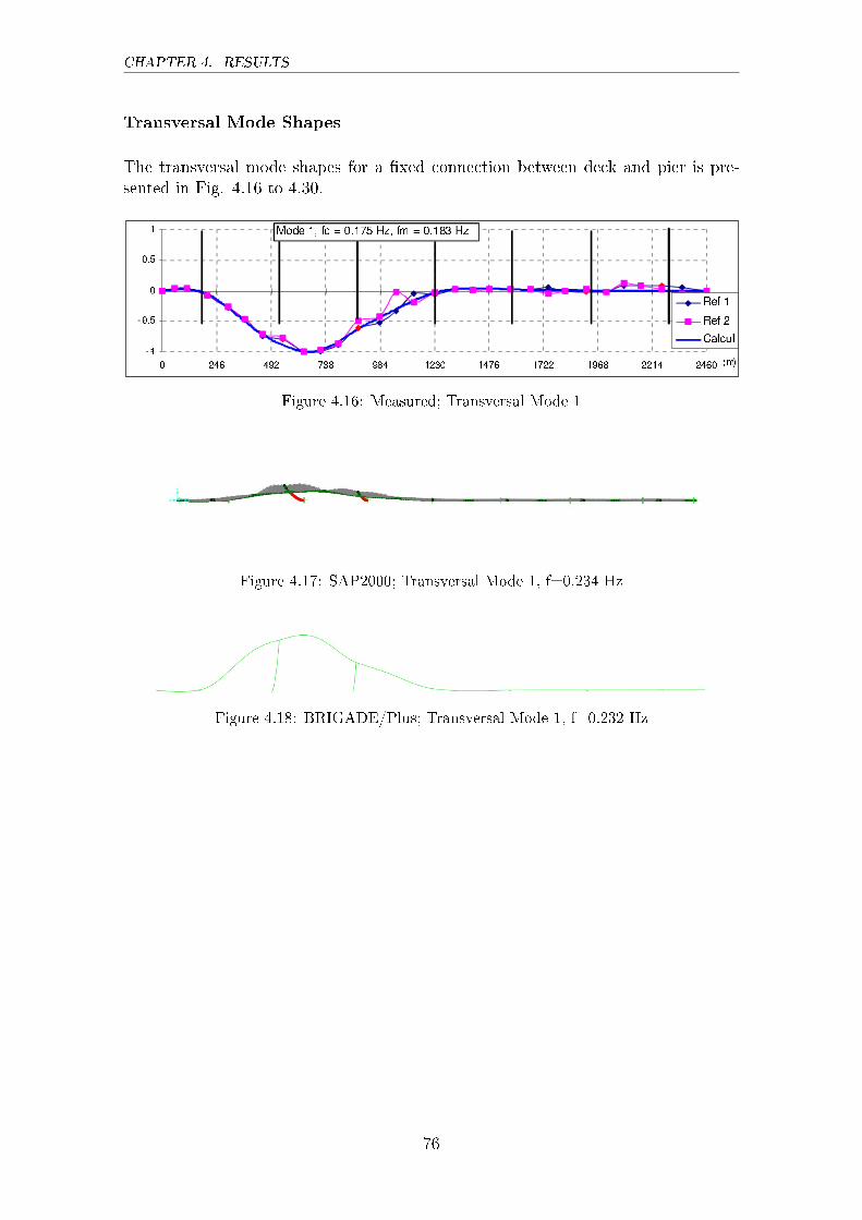
CHAPTER 4. RESULTS
Transversal Mode Shapes
The transversal mode shapes for a �xed connection between deck and pier is pre-sented in Fig. 4.16 to 4.30.
Figure 4.16: Measured; Transversal Mode 1
Figure 4.17: SAP2000; Transversal Mode 1, f=0.234 Hz
Figure 4.18: BRIGADE/Plus; Transversal Mode 1, f=0.232 Hz
76
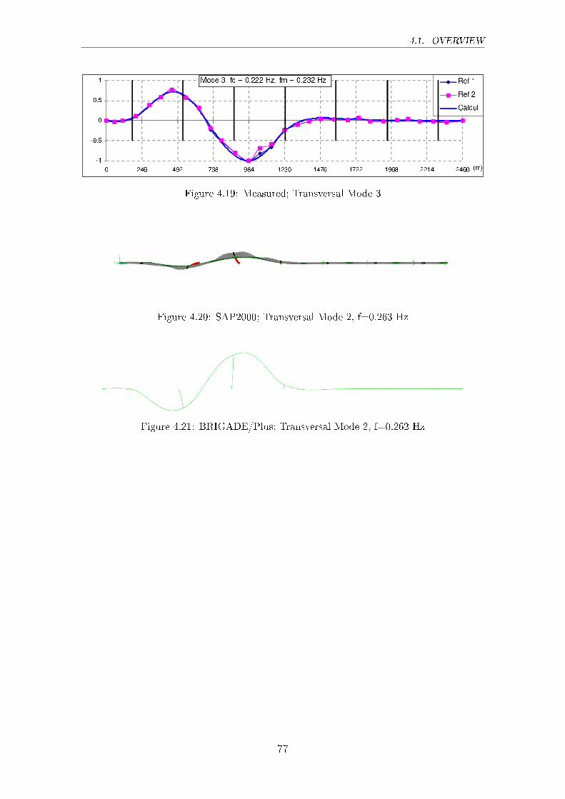
4.1. OVERVIEW
Figure 4.19: Measured; Transversal Mode 3
Figure 4.20: SAP2000; Transversal Mode 2, f=0.263 Hz
Figure 4.21: BRIGADE/Plus; Transversal Mode 2, f=0.262 Hz
77

CHAPTER 4. RESULTS
Figure 4.22: Measured; Transversal Mode 5
Figure 4.23: SAP2000; Transversal Mode 5, f=0.372 Hz
Figure 4.24: BRIGADE/Plus; Transversal Mode 3, f=0.359 Hz
78
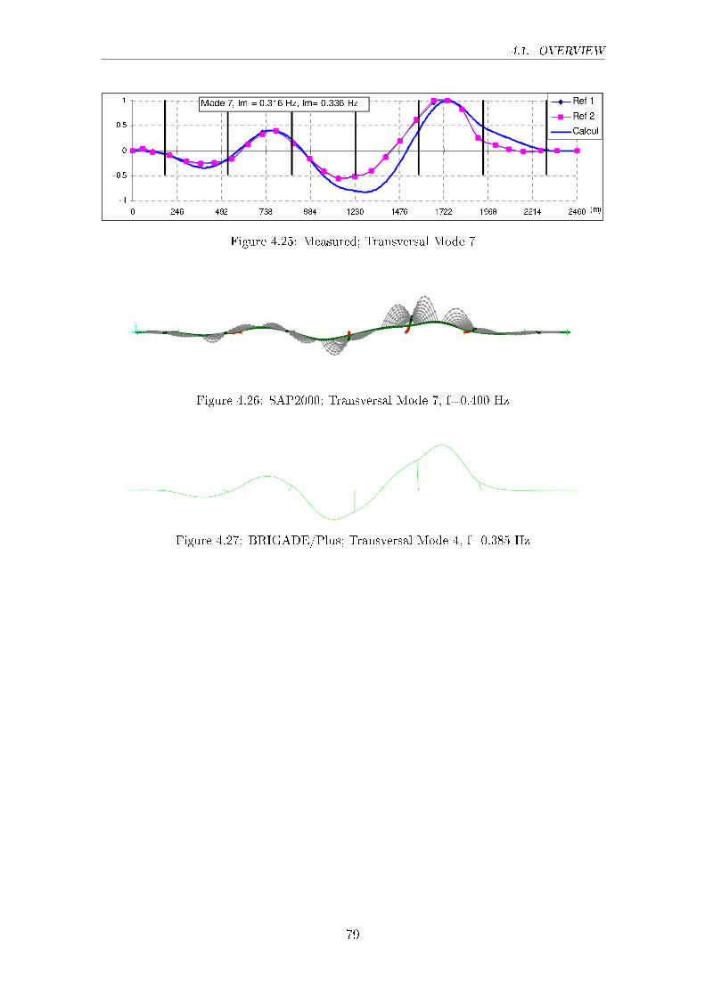
4.1. OVERVIEW
Figure 4.25: Measured; Transversal Mode 7
Figure 4.26: SAP2000; Transversal Mode 7, f=0.400 Hz
Figure 4.27: BRIGADE/Plus; Transversal Mode 4, f=0.385 Hz
79
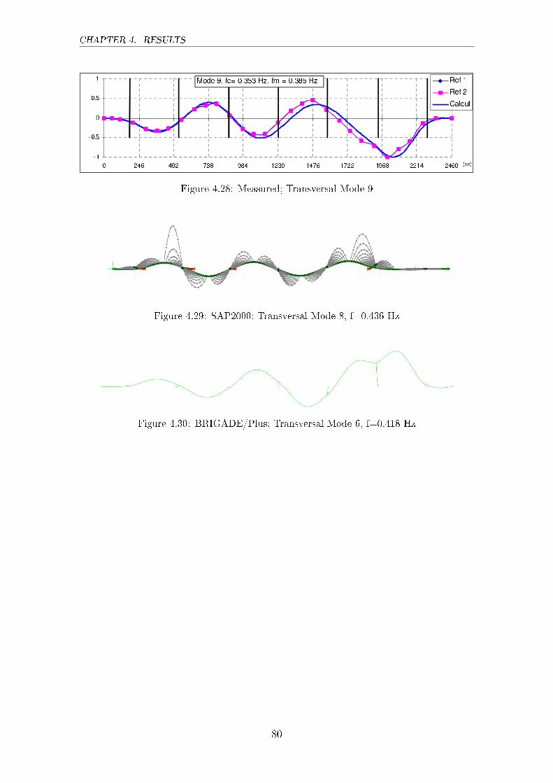
CHAPTER 4. RESULTS
Figure 4.28: Measured; Transversal Mode 9
Figure 4.29: SAP2000; Transversal Mode 8, f=0.436 Hz
Figure 4.30: BRIGADE/Plus; Transversal Mode 6, f=0.418 Hz
80
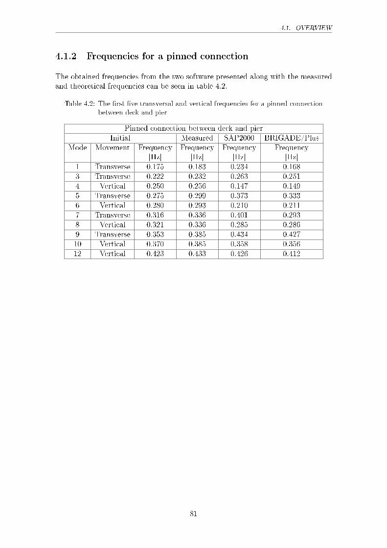
4.1. OVERVIEW
4.1.2 Frequencies for a pinned connection
The obtained frequencies from the two software presented along with the measuredand theoretical frequencies can be seen in table 4.2.
Table 4.2: The �rst �ve transversal and vertical frequencies for a pinned connectionbetween deck and pier
Pinned connection between deck and pierInitial Measured SAP2000 BRIGADE/Plus
Mode Movement Frequency Frequency Frequency Frequency[Hz] [Hz] [Hz] [Hz]
1 Transverse 0.175 0.183 0.234 0.1683 Transverse 0.222 0.232 0.263 0.2514 Vertical 0.250 0.256 0.147 0.1495 Transverse 0.275 0.299 0.373 0.3336 Vertical 0.280 0.293 0.210 0.2117 Transverse 0.316 0.336 0.401 0.2938 Vertical 0.321 0.336 0.285 0.2869 Transverse 0.353 0.385 0.434 0.42710 Vertical 0.370 0.385 0.358 0.35612 Vertical 0.423 0.433 0.426 0.412
81
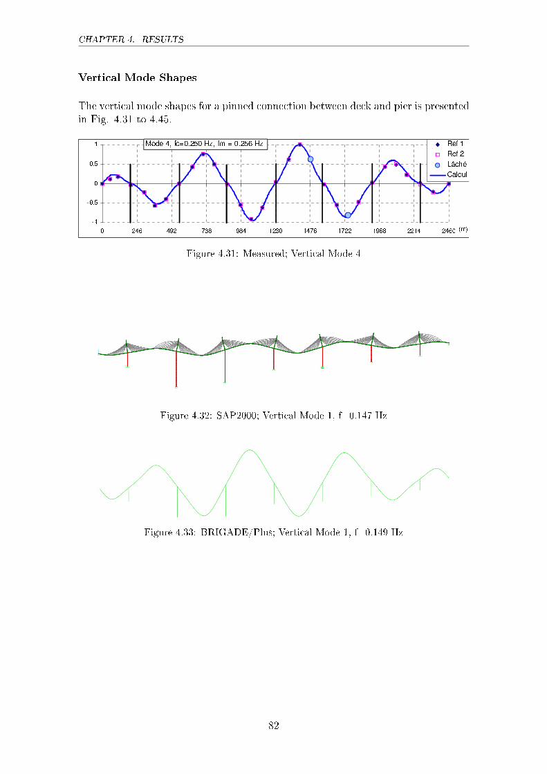
CHAPTER 4. RESULTS
Vertical Mode Shapes
The vertical mode shapes for a pinned connection between deck and pier is presentedin Fig. 4.31 to 4.45.
Figure 4.31: Measured; Vertical Mode 4
Figure 4.32: SAP2000; Vertical Mode 1, f=0.147 Hz
Figure 4.33: BRIGADE/Plus; Vertical Mode 1, f=0.149 Hz
82
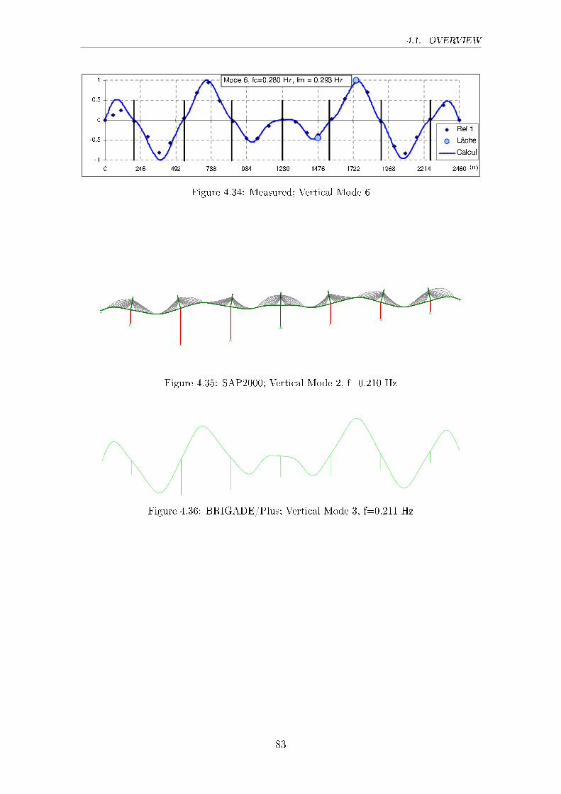
4.1. OVERVIEW
Figure 4.34: Measured; Vertical Mode 6
Figure 4.35: SAP2000; Vertical Mode 2, f=0.210 Hz
Figure 4.36: BRIGADE/Plus; Vertical Mode 3, f=0.211 Hz
83
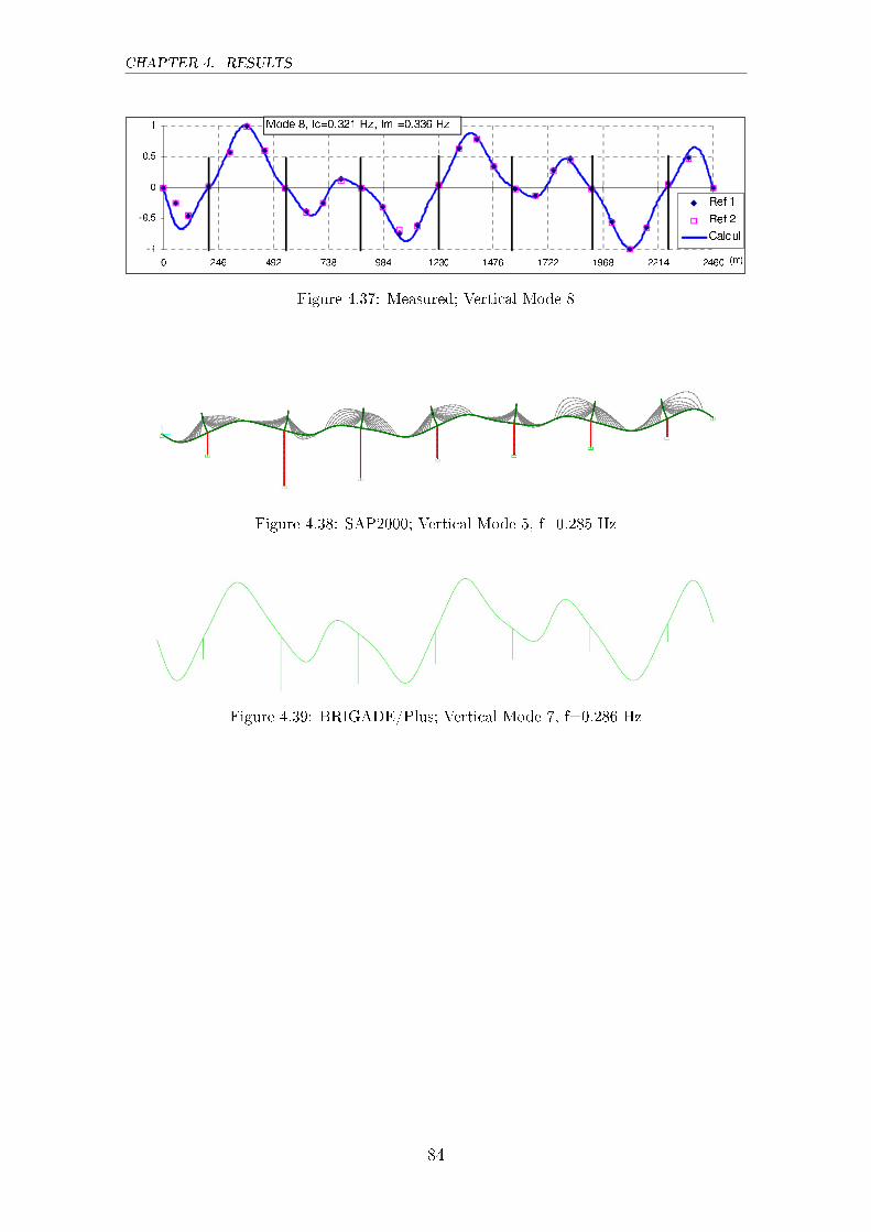
CHAPTER 4. RESULTS
Figure 4.37: Measured; Vertical Mode 8
Figure 4.38: SAP2000; Vertical Mode 5, f=0.285 Hz
Figure 4.39: BRIGADE/Plus; Vertical Mode 7, f=0.286 Hz
84
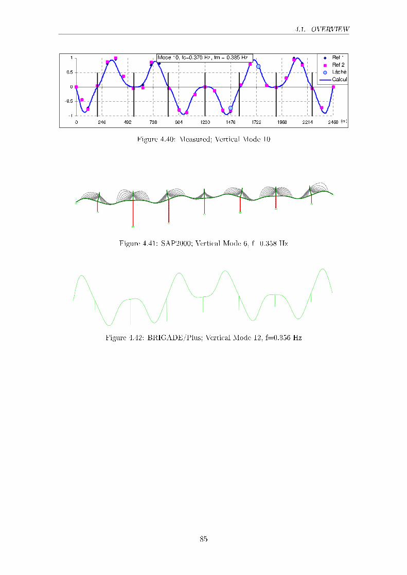
4.1. OVERVIEW
Figure 4.40: Measured; Vertical Mode 10
Figure 4.41: SAP2000; Vertical Mode 6, f=0.358 Hz
Figure 4.42: BRIGADE/Plus; Vertical Mode 12, f=0.356 Hz
85
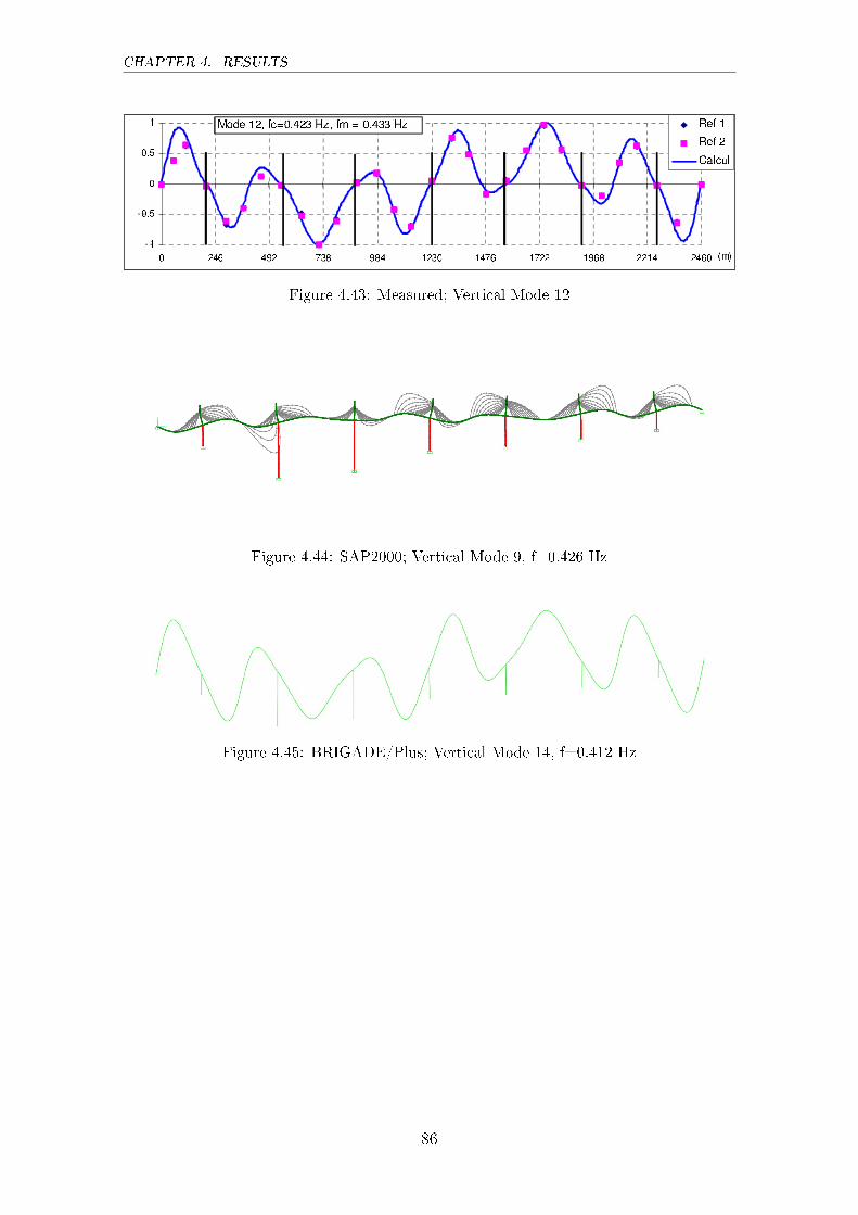
CHAPTER 4. RESULTS
Figure 4.43: Measured; Vertical Mode 12
Figure 4.44: SAP2000; Vertical Mode 9, f=0.426 Hz
Figure 4.45: BRIGADE/Plus; Vertical Mode 14, f=0.412 Hz
86
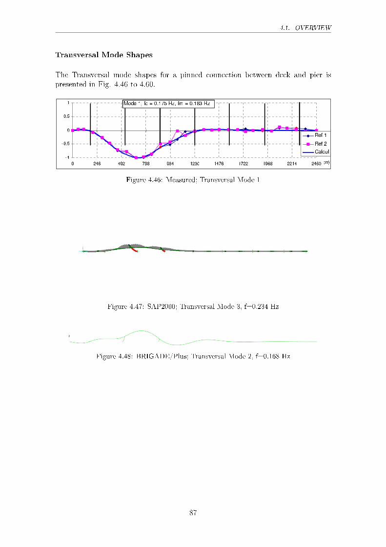
4.1. OVERVIEW
Transversal Mode Shapes
The Transversal mode shapes for a pinned connection between deck and pier ispresented in Fig. 4.46 to 4.60.
Figure 4.46: Measured; Transversal Mode 1
Figure 4.47: SAP2000; Transversal Mode 3, f=0.234 Hz
Figure 4.48: BRIGADE/Plus; Transversal Mode 2, f=0.168 Hz
87
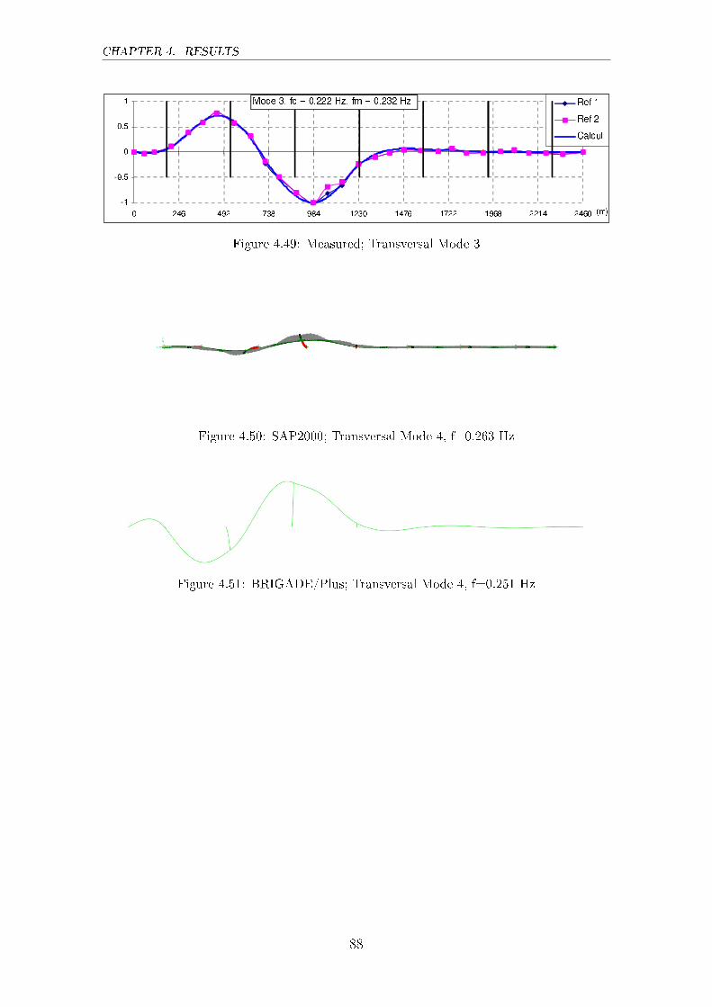
CHAPTER 4. RESULTS
Figure 4.49: Measured; Transversal Mode 3
Figure 4.50: SAP2000; Transversal Mode 4, f=0.263 Hz
Figure 4.51: BRIGADE/Plus; Transversal Mode 4, f=0.251 Hz
88
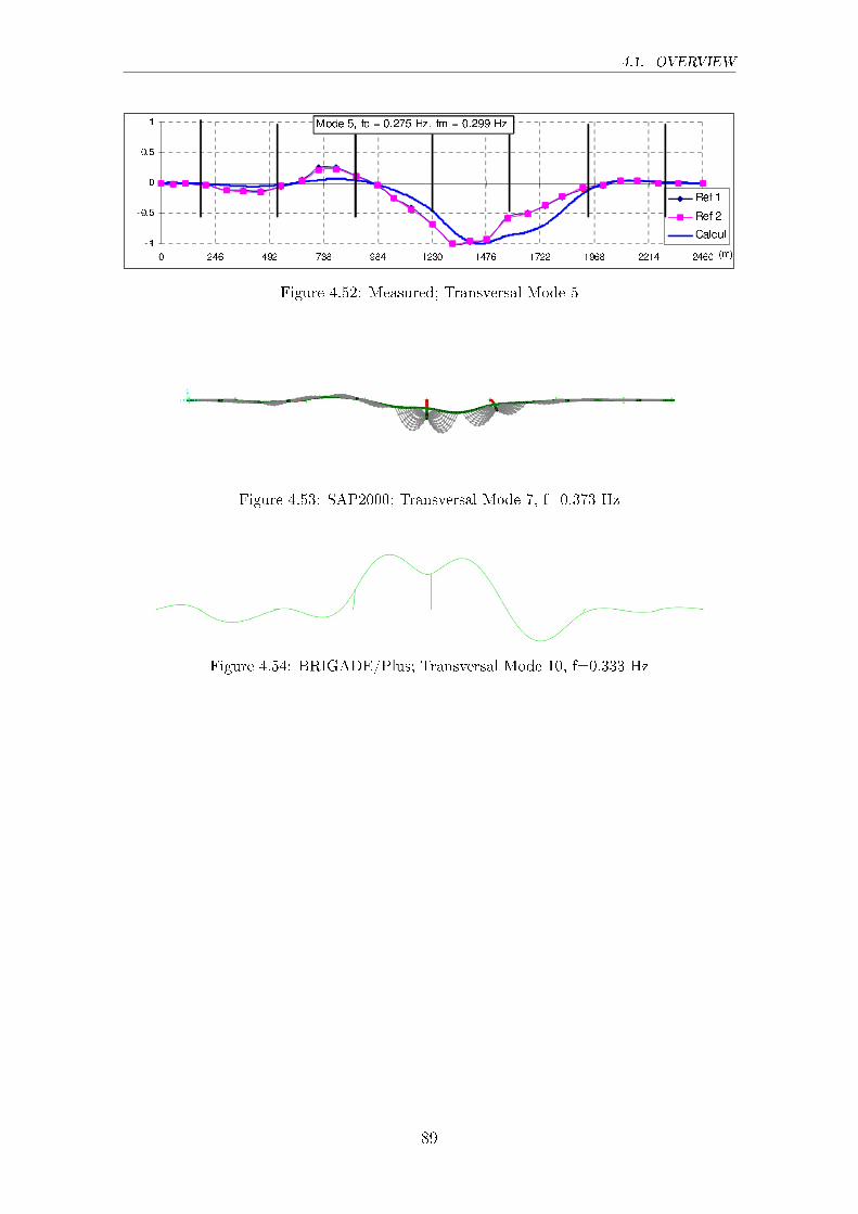
4.1. OVERVIEW
Figure 4.52: Measured; Transversal Mode 5
Figure 4.53: SAP2000; Transversal Mode 7, f=0.373 Hz
Figure 4.54: BRIGADE/Plus; Transversal Mode 10, f=0.333 Hz
89
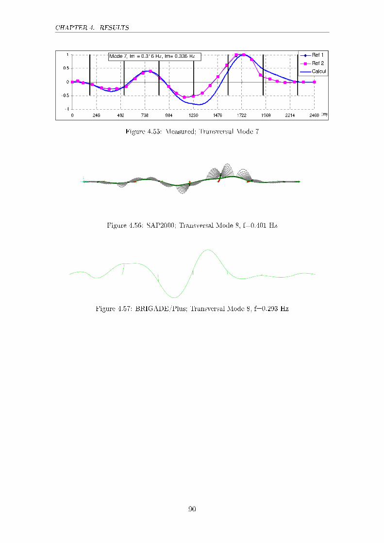
CHAPTER 4. RESULTS
Figure 4.55: Measured; Transversal Mode 7
Figure 4.56: SAP2000; Transversal Mode 8, f=0.401 Hz
Figure 4.57: BRIGADE/Plus; Transversal Mode 8, f=0.293 Hz
90
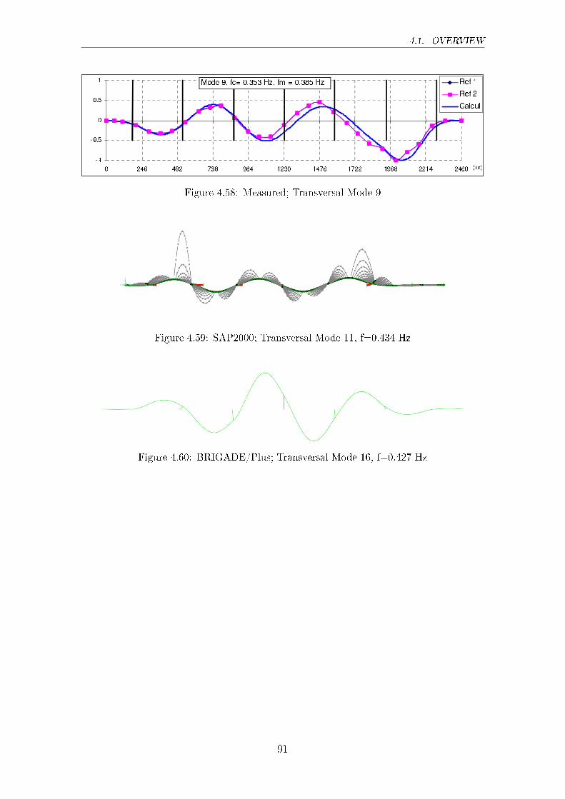
4.1. OVERVIEW
Figure 4.58: Measured; Transversal Mode 9
Figure 4.59: SAP2000; Transversal Mode 11, f=0.434 Hz
Figure 4.60: BRIGADE/Plus; Transversal Mode 16, f=0.427 Hz
91

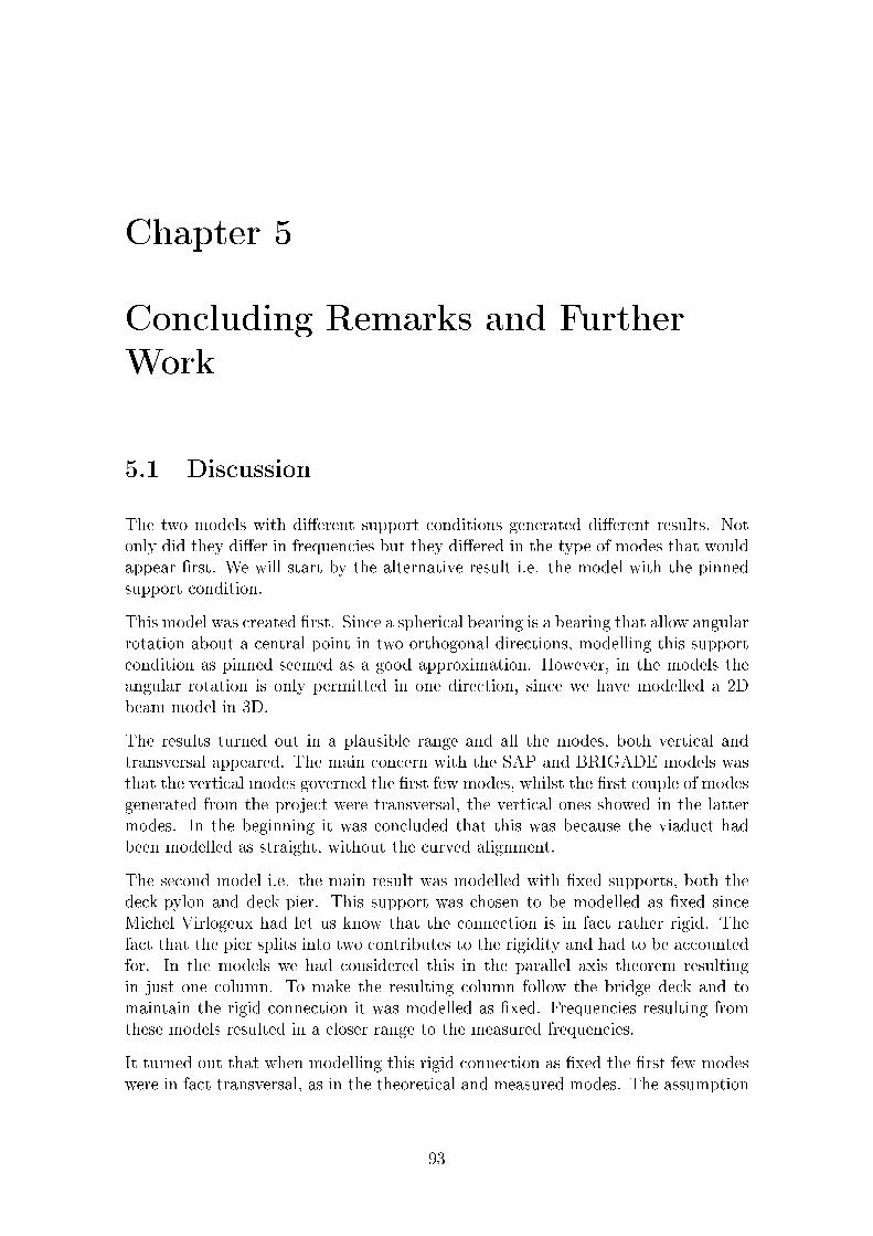
Chapter 5
Concluding Remarks and Further
Work
5.1 Discussion
The two models with di�erent support conditions generated di�erent results. Notonly did they di�er in frequencies but they di�ered in the type of modes that wouldappear �rst. We will start by the alternative result i.e. the model with the pinnedsupport condition.
This model was created �rst. Since a spherical bearing is a bearing that allow angularrotation about a central point in two orthogonal directions, modelling this supportcondition as pinned seemed as a good approximation. However, in the models theangular rotation is only permitted in one direction, since we have modelled a 2Dbeam model in 3D.
The results turned out in a plausible range and all the modes, both vertical andtransversal appeared. The main concern with the SAP and BRIGADE models wasthat the vertical modes governed the �rst few modes, whilst the �rst couple of modesgenerated from the project were transversal, the vertical ones showed in the lattermodes. In the beginning it was concluded that this was because the viaduct hadbeen modelled as straight, without the curved alignment.
The second model i.e. the main result was modelled with �xed supports, both thedeck-pylon and deck-pier. This support was chosen to be modelled as �xed sinceMichel Virlogeux had let us know that the connection is in fact rather rigid. Thefact that the pier splits into two contributes to the rigidity and had to be accountedfor. In the models we had considered this in the parallel axis theorem resultingin just one column. To make the resulting column follow the bridge deck and tomaintain the rigid connection it was modelled as �xed. Frequencies resulting fromthese models resulted in a closer range to the measured frequencies.
It turned out that when modelling this rigid connection as �xed the �rst few modeswere in fact transversal, as in the theoretical and measured modes. The assumption
93
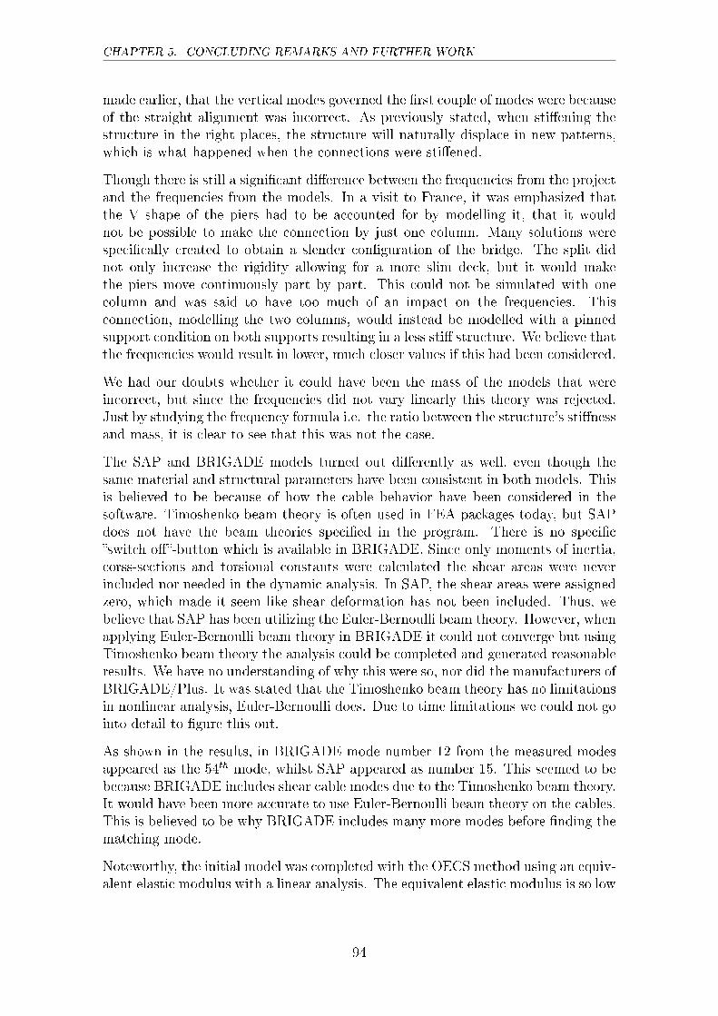
CHAPTER 5. CONCLUDING REMARKS AND FURTHER WORK
made earlier, that the vertical modes governed the �rst couple of modes were becauseof the straight alignment was incorrect. As previously stated, when sti�ening thestructure in the right places, the structure will naturally displace in new patterns,which is what happened when the connections were sti�ened.
Though there is still a signi�cant di�erence between the frequencies from the projectand the frequencies from the models. In a visit to France, it was emphasized thatthe V shape of the piers had to be accounted for by modelling it, that it wouldnot be possible to make the connection by just one column. Many solutions werespeci�cally created to obtain a slender con�guration of the bridge. The split didnot only increase the rigidity allowing for a more slim deck, but it would makethe piers move continuously part by part. This could not be simulated with onecolumn and was said to have too much of an impact on the frequencies. Thisconnection, modelling the two columns, would instead be modelled with a pinnedsupport condition on both supports resulting in a less sti� structure. We believe thatthe frequencies would result in lower, much closer values if this had been considered.
We had our doubts whether it could have been the mass of the models that wereincorrect, but since the frequencies did not vary linearly this theory was rejected.Just by studying the frequency formula i.e. the ratio between the structure's sti�nessand mass, it is clear to see that this was not the case.
The SAP and BRIGADE models turned out di�erently as well, even though thesame material and structural parameters have been consistent in both models. Thisis believed to be because of how the cable behavior have been considered in thesoftware. Timoshenko beam theory is often used in FEA packages today, but SAPdoes not have the beam theories speci�ed in the program. There is no speci�c�switch o��-button which is available in BRIGADE. Since only moments of inertia,corss-sections and torsional constants were calculated the shear areas were neverincluded nor needed in the dynamic analysis. In SAP, the shear areas were assignedzero, which made it seem like shear deformation has not been included. Thus, webelieve that SAP has been utilizing the Euler-Bernoulli beam theory. However, whenapplying Euler-Bernoulli beam theory in BRIGADE it could not converge but usingTimoshenko beam theory the analysis could be completed and generated reasonableresults. We have no understanding of why this were so, nor did the manufacturers ofBRIGADE/Plus. It was stated that the Timoshenko beam theory has no limitationsin nonlinear analysis, Euler-Bernoulli does. Due to time limitations we could not gointo detail to �gure this out.
As shown in the results, in BRIGADE mode number 12 from the measured modesappeared as the 54th mode, whilst SAP appeared as number 15. This seemed to bebecause BRIGADE includes shear cable modes due to the Timoshenko beam theory.It would have been more accurate to use Euler-Bernoulli beam theory on the cables.This is believed to be why BRIGADE includes many more modes before �nding thematching mode.
Noteworthy, the initial model was completed with the OECS method using an equiv-alent elastic modulus with a linear analysis. The equivalent elastic modulus is so low
94

5.1. DISCUSSION
that the truss element used to simulate the cable will not behave in a linear elasticmanner, but will adopt a small sag only allowing for tension, assuming a parabolicshape. This modulus will be low enough to not be able to resist compression. Wechose to complete a nonlinear analysis with the MECS method using beam elements.We believe that by using this method we would obtain a better approximation of thereality. By meshing the cables they will adopt a more realistic shape, forming theshape of a catenary. Additionally, since a lumped mass matrix is used in SAP andBRIGADE, a �ner mesh will create a more consistent �ner distribution of each �niteelement. The beam element also simulated the cable behavior better than a singletruss element, due to the bending sti�ness which will carry the cable self-weight.This will ultimately include the cable vibrations that the OECS method precludes.This has also had an impact on the results. The OECS method is perhaps a goodapproximation, but since our primary aim was to come as close to reality as possible,the MECS method seemed most reasonable to adopt.
95
CHAPTER 5. CONCLUDING REMARKS AND FURTHER WORK
5.2 Conclusions
Two models were analyzed, the pinned connection and the �xed connection betweenthe deck and pier, both modelling the pier with one column. Due to the spheri-cal bearings permitting angular rotation, this was simulated by adopting a pinnedconnection. This resulted in the �rst few modes being primarily vertical. This wasbelieved to be due to that the curved alignment of the bridge had been neglected.In order to get the structural mechanics correct as this connection is rigid, this wasinstead modelled as �xed. The shapes of the �rst couple of modes turned out to betransversal. It could be concluded that not modelling the curved alignment did nothave the big impact that we thought from the beginning.
After an analysis of our results, it was concluded that the speci�c V shaped connec-tion had to be modelled as two columns to simulate the correct behavior. This isassumed to be a key feature to the �right� frequencies.
As for the di�erences in the results between the programs, we believe that applyingTimoshenko beam theory in BRIGADE lead to that shear cable vibrations wereincluded. Timoshenko is more sensitive towards cable vibrations and the morecorrect way to handle this would have been to apply Euler-Bernoulli to the cables.
By using the MECS method and a meshing scheme of eight �nite elements we believethat we have made a more realistic approximation of the cable as it adopts a catenaryshape simulating the sag. Even though beam elements can resist both bending andcompression, which a cable cannot. This bending sti�ness is necessary to carry theself-weight. The MECS method is also capable to show the cable vibrations that isprecluded in OECS method.
Additionally, the option to assign the beam elements the ability to resist tensiononly was applied. This way of modelling the cables were evaluated to be the mostaccurate way to approximate the reality.
96
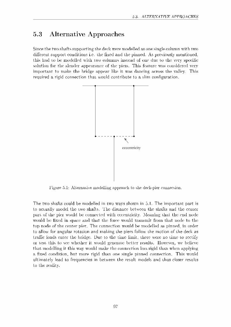
5.3. ALTERNATIVE APPROACHES
5.3 Alternative Approaches
Since the two shafts supporting the deck were modelled as one single column with twodi�erent support conditions i.e. the �xed and the pinned. As previously mentioned,this had to be modelled with two columns instead of one due to the very speci�csolution for the slender appearance of the piers. This feature was considered veryimportant to make the bridge appear like it was dancing across the valley. Thisrequired a rigid connection that would contribute to a slim con�guration.
eccentricity
Figure 5.1: Alternative modelling approach to the deck-pier connection.
The two shafts could be modelled in two ways shown in 5.1. The important part isto actually model the two shafts. The distance between the shafts and the centerpart of the pier would be connected with eccentricity. Meaning that the end nodewould be �xed in space and that the force would transmit from that node to thetop node of the center pier. The connection would be modelled as pinned, in orderto allow for angular rotation and making the piers follow the motion of the deck astra�c loads enter the bridge. Due to the time limit, there were no time to rectifyor test this to see whether it would generate better results. However, we believethat modelling it this way would make the connection less rigid than when applyinga �xed condition, but more rigid than one single pinned connection. This wouldultimately lead to frequencies in between the result models and thus closer resultsto the reality.
97

Bibliography
Abdel-Gha�ar, A., Khalifa, M., 1991. Importance of cable vibration in dynamics ofcable-stayed bridges. ASCE Journal of Engineering Mechanics 117, 2571�2589.
Abdel-Gha�ar, A., Nazmy, A., 1991. 3-D nonlinear seismic behavior of cable-stayedbridges. Journal of Structural Engineering 117, No. 11, 3456�3476.
Asgari, B., Osman, S., Adnan, A., 2013. Three-dimensional �nite element modellingof long-span cable-stayed bridges. The IES Journal 6, No. 4, 258�269.
Au, F., Cheng, Y., Cheung, Y., Zheng, D., 2001. On the determination of naturalfrequencies and mode shapes of cable-stayed bridges. Mathematical Modelling 25,1099�1115.
Autodesk, 2016. Metrics and the basics of mechanics.http://sustainabilityworkshop.autodesk.com, accessed: 2016-06-01.
Bauchau, O., Craig, J., 2009. Structural Analysis, With Applications to AerospaceStructures. Springer Dordrecht Heidelberg, London, New York.
Chopra, A. K., 2012. Dynamics of Structures, Theory and Applications to Earth-quake Engineering, 4th Edition. University of California at Berkeley, USA.
Chung, C., Wang, S., 2015. Computational Analysis and Design of Bridge Struc-tures. Taylor and Francis Group, USA.
Cook, R. D., Malkus, D. S., Plesha, M. E., Witt, R. J., 2002. Concept and Ap-plications of Finite Element Analysis, 4th Edition. John Wiley and Sons, Ltd,USA.
CSI, 2016. Sap2000. https://www.csiamerica.com/products/sap2000, accessed:2016-05-17.
CSIAmerica, 2015. SAP2000, CSI Analysis Reference Manual. Barkeley, California,USA, 17th Edition.
DelForno, 2001. Drawing. Accessed: 2016.
Ernst, H., 1965. Der e-modul von seilen unter berücksichtigung des Durchanges. DerBauingenieur 40.
Fleming, J., 1979. Nonlinear static analysis of cable-stayed bridge structures. Com-puters and Structures 10, 621�635.
99
BIBLIOGRAPHY
Freire, A., Negrao, J., Lopes, A., 2006. Geometrical nonlinearites on the staticanalysis of highly �exible steel cable-stayed bridges. Computers and Structures84, 2128�2140.
Gimsing, N. J., 1998. Cable Supported Bridges, Concept and Design, 2nd Edition.John Wiley and Sons, Ltd, USA.
Greisch, 2001. Drawing. Accessed: 2016.
Hajdin, N., Michaltsos, G., T.G., K., 1998. About the equivalent modulus of elas-ticity of cables of cable-stayed bridges. Facta Universitatis 1, No. 5, 569�575.
Hall, C., 2016. Linkedin, modal analysis - shake, rattle and roll!https://www.linkedin.com, accessed: 2016-06-01.
Heyden, S., Dahlblom, O., Olsson, A., Sandberg, G., 2008. Introduktion till Struk-turmekaniken, 4th Edition. Studentlitteratur, Sverige.
Liu, M., Lin, L., Wang, P., 2014. Deck-stay interaction with appropriate initialshapes of cable-stayed bridges. Engineering Computations 31, 634�655.
Roadtra�c-Technology, 2016. Millau Viaduct, France. Accessed: 2016-05-25.
Scanscot, 2016. Scanscot. https://scanscot.com, accessed: 2016-05-17.
SIMULIA, 2011. ABAQUS 6.11. USA.
Sönnerlind, H., 2016. Geometric nonlinearity. Accessed: 2016-04-20.
Strang, G., 2016. Introduction to Linear Algebra, 5th Edition. Massachusetts Insti-tute of Technology, Cambridge, Massachusetts USA.
Sundquist, H., 2010. Cable supported structures, 3rd Edition. Div. for StructuralDesign and Bridges Royal Institute of Technology, Stockholm.
Unknown, 2016. Highest bridges. http://www.highestbridges.com, accessed: 2016-06-01.
Virlogeux, M., 2000. The viaduct over the River Tarn at Millau.
Virlogeux, M., Cachot, E., Vayssade, T., Lancon, H., Hajar, Z., Servant, C., 2015.The Millau Viaduct: Ten years of structural monitoring. Structural EngineeringInternational 25, 375�380.
Wang, P., Lin, H., Tang, T., 2002. Study on nonlinear analysis of a highly redundantcable-stayed bridge. Computers and Structures 80, 165�182.
Wang, P., Tseng, T., Yang, C., 1993. Initial shape of cable-stayed bridges. Computersand Structures 46, No. 6, 1095�1106.
Wang, P., Yang, C., 1996. Parametic studies on cable-stayed bridges. Computersand Structures 60, No. 2, 243�260.
100

BIBLIOGRAPHY
Wikipedia, 2016. Timoshenko beam theory. https://en.wikipedia.org, accessed:2016-06-01.
Zhu, L., Xiang, H., Xu, Y., 2000. Triple-girder model for modal analysis of cable-stayed bridges with warping e�ect. Engineering and Structural 22, 1313�1323.
101

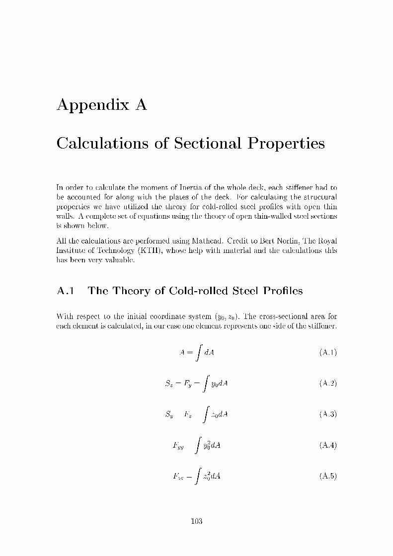
Appendix A
Calculations of Sectional Properties
In order to calculate the moment of Inertia of the whole deck, each sti�ener had tobe accounted for along with the plates of the deck. For calculating the structuralproperties we have utilized the theory for cold-rolled steel pro�les with open thinwalls. A complete set of equations using the theory of open thin-walled steel sectionsis shown below.
All the calculations are performed using Mathcad. Credit to Bert Norlin, The RoyalInstitute of Technology (KTH), whose help with material and the calculations thishas been very valuable.
A.1 The Theory of Cold-rolled Steel Pro�les
With respect to the initial coordinate system (y0; z0), The cross-sectional area foreach element is calculated, in our case one element represents one side of the sti�ener.
A =
ZdA (A.1)
Sz = Fy =
Zy0dA (A.2)
Sy = Fz =
Zz0dA (A.3)
Fyy =
Zy20dA (A.4)
Fzz =
Zz20dA (A.5)
103
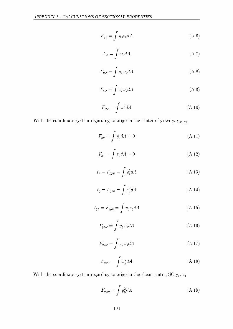
APPENDIX A. CALCULATIONS OF SECTIONAL PROPERTIES
Fyz =
Zy0z0dA (A.6)
F! =
Z!0dA (A.7)
Fy! =
Zy0!0dA (A.8)
Fz! =
Zz0!0dA (A.9)
F!! =
Z!20dA (A.10)
With the coordinate system regarding to origo in the center of gravity, yg, zg
Fgy =
ZygdA = 0 (A.11)
Fgz =
ZzgdA = 0 (A.12)
Iz = Fgyy =
Zy2gdA (A.13)
Iy = Fgzz =
Zz2gdA (A.14)
Iyz = Fgyz =
ZygzgdA (A.15)
Fgy! =
Zyg!gdA (A.16)
Fgz! =
Zzg!gdA (A.17)
Fg!! =
Z!2gdA (A.18)
With the coordinate system regarding to origo in the shear centre, SC ys, zs
F�yy =
Zy2�dA (A.19)
104
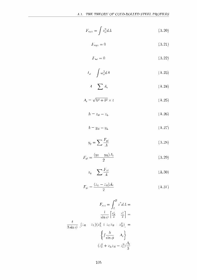
A.1. THE THEORY OF COLD-ROLLED STEEL PROFILES
F�zz =
Zz2�dA (A.20)
F�yz = 0 (A.21)
Fs! = 0 (A.22)
I! =
Z!2sdA (A.23)
A =X
Ai (A.24)
Ai =ph2 + b2 � t (A.25)
h = zR � zL (A.26)
b = yR � yL (A.27)
yg =X Fyi
A(A.28)
Fyi =(yL + yR)Ai
2(A.29)
zg =X Fzi
A(A.30)
Fzi =(zL + zR)Ai
2(A.31)
Fzzi =
Z R
L
z2dA =
t
sin
hz3R3� z3L
3
i=
t
3 sin
�(zR � zL)(z
2L + zLzR + z2R)
�=�
fh
sin�= Ai
�=
(z2L + zLzR + z2r )Ai
3
105
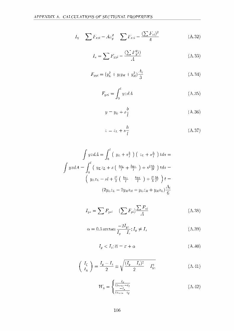
APPENDIX A. CALCULATIONS OF SECTIONAL PROPERTIES
Iy =X
Fzzi � Az2g =X
Fzzi � (PFzi)
2
A(A.32)
Iz =X
Fyyi �(PF 2yi)
A(A.33)
Fyyi = (y2L + ylyR + y2R)Ai
3(A.34)
Fyzi =
Z l
0
yzdA (A.35)
y = yL + sb
l(A.36)
z = zL + sh
l(A.37)
ZyzdA =
Z l
0
�yL + s b
l
� �zL + sh
l
�tds =Z
yzdA =
Z l
0
�yLzL + s
�bzLl
+ hyLl
�+ s2 bh
l2
�tds =�
yLzL + sl + l2
2
�bzLl
+ hyLl
�+ l3
3bhl2
�t =
(2yLzL + 2yRzR + yLzR + yRzL)Ai
6
Iyz =X
Fyzi � (X
Fyi)
PFzi
A(A.38)
� = 0:5 arctan�2IyzIy � Iz
; Iy 6= Iz (A.39)
Iy < Iz;� = � + � (A.40)
�I�I�
�=Iy + Iz
2�r
(Iy � Iz)2
2+ I2yz (A.41)
Wy =
(Iy
(zmax�zg�Iy
(zmin�zg
(A.42)
106

A.1. THE THEORY OF COLD-ROLLED STEEL PROFILES
Wz =
(Iz
(ymax�yg�Iz
(ymin�yg
(A.43)
107