a simple model of demand-led growth and income...

A Simple Model of Demand-Led

Growth and Income Distribution

Nelson H. Barbosa-Filho

Institute of Economics, Federal University of Rio de Janeiro(IE/UFRJ), Brazil

AbstractThis paper presents a one-sector demand-led model where capital

and non-capital expenditures determine income growth and distribu-tion. The basic idea is to build a simple dynamical accounting modelfor the growth rate of the capital stock, the ratio of non-capital ex-penditures to the capital stock, and the labor share of income. By in-serting some stylized behavioral functions in the identities, the paperanalyzes the implications of alternative theoretical closures of incomedetermination (effective demand) and distribution (social conflict).On the demand side, two behavioral functions define the growth ratesof capital and non-capital expenditures in terms of capacity utiliza-tion (measured by the output-capital ratio) and income distribution(measured by the labor share of income). On the distribution side,another two behavioral functions describe the growth rates of the realwage and labor productivity also in terms of capacity utilization andincome distribution. The growth rates of multifactor productivity andemployment follow residually from the accounting identities and, inthis way, the demand-led model can encompass supply-driven modelsas a special case.

Keywords: Demand-led Growth, Effective Demand, IncomeDistribution

Revista EconomiA December 2004


JEL Classification: E250, E320, O400, O410

Este artigo apresenta um modelo de um setor onde os gastoscorrentes e de capital determinam o crescimento e a distribuicaoda renda. A ideia basica e construir um modelo contabil simplese dinamico para a taxa de crescimento do estoque de capital, arazao entre gastos correntes e estoque de capital, e a parcela sala-rial da renda. Mediante a insercao de algumas funcoes compor-tamentais estilizadas nas identidades contabeis, o artigo analisaas implicacoes de fechamentos teoricos alternativos para a de-terminacao (demanda efetiva) e distribuicao (conflito social) darenda. Do lado da demanda, duas equacoes definem as taxas decrescimento das despesas correntes e de capital como funcoes dograu de utilizacao da capacidade produtiva (medida pela relacaorenda-capital) e distribuicao de renda (medida pela parcela sa-larial da renda). Do lado da distribuicao, outras duas equacoesdescrevem as taxas de crescimento do salario real e da produ-tividade do trabalho tambem como funcoes do grau de utilizacaoda capacidade produtiva e da distribuicao de renda. A taxa decrescimento do emprego e da produtividade total dos fatores saoobtidas residualmente das identidades contabeis e, desta forma,o modelo liderado pela demanda pode incluir modelos lideradospela oferta como casos especiais.

Email address: [email protected] (Nelson H.Barbosa-Filho).

118 EconomiA, Selecta, Brasılia(DF), v.5, n.3, p.117–154, Dec. 2004

A Simple Model of Demand-Led Growth and Income Distribution

“One of the major weakness in the core ofmacroeconomics as I represented it is the lack of real

coupling between the short-run picture and the long-runpicture.” Robert Solow (1997, p.231).

1 Introduction

Modern macroeconomic theory has a strange way to deal witheconomic growth. When analyzing short-run issues, most econ-omists tend to explain income variations in terms of changes inaggregate demand. When dealing with long-run issues, the fo-cus changes to aggregate supply and the analysis shifts to thedeterminants of potential output in some sort of growth account-ing based on the Solow-Swan model. Exactly how effective andpotential income levels converge in the long run is not usuallystated clearly in supply-driven growth models. Instead, it is usu-ally assumed that, either because of government intervention orbecause of the self-adjusting nature of market forces, capitalisteconomies tend to operate at their potential income level in thelong run. If so, one can then understand growth just from thesupply side and effective demand vanishes from long-run macroe-conomic theory.

Independently of the importance of supply issues, the empha-sis of modern growth theory on potential output tends to ignorethe fact that capitalist economies may stay below their maximumoutput for long periods of time. Even if one accepts Say’s law andassumes that effective demand does converge to potential outputin the long run, the adjusting period may be long enough to makea demand-led growth theory worthy for medium-run macroeco-nomics. In the words of Solow (1997), p.230: “(...) what aboutthose fluctuations around the trend of potential output? (...) In

EconomiA, Selecta, Brasılia(DF), v.5, n.3, p.117–154, Dec. 2004 119


my picture of the usable core of macroeconomics, those fluctu-ations are predominantly driven by aggregate demand impulsesand the appropriate vehicle for analyzing them is some modelof the various sources of expenditures.” If one rejects Say’s lawand assumes instead that it is potential output that convergesto effective demand in the long run, the need for a demand-ledgrowth theory becomes even more obvious.

The demand determination of income is a point usually em-phasized by post Keynesian and structuralist economists. Build-ing upon the works of Keynes (1936) and Kalecki (1971), theseeconomists tend to analyze growth in terms of the dynamics ofautonomous expenditures under the assumption that potentialoutput itself may be demand-driven. The basic idea is that effec-tive demand may determine the growth rate of potential outputthrough its effects on the capital stock and multifactor produc-tivity. 1 If income growth is mainly demand-driven, the focus ofthe analysis shifts to the determinants of effective demand. In thepost Keynesian and structuralist literature the usual suspects areincome distribution, macroeconomic policy, and the autonomousdemand coming from the private or the foreign sectors. 2 Thestructure of the models varies according to which source of de-mand is supposed to drive income and this tends to be an obsta-cle for the wider use of such models in applied macroeconomics.

1 Effective demand is also assumed to influence the labor supplythrough changes in the labor-force participation rate. However, be-cause this rate cannot obviously be higher than 100%, this trans-mission mechanism from demand to labor supply is limited withoutmigration.2 For methodological discussion of the role of aggregate demand andsupply in growth theory, see Leon-Ledesma and Thirlwall (2000),Panico (2003), and Solow (1997), Solow (2000). For a survey of Key-nesian demand-led growth models, see, for instance, Commendatoreet al. (2003).



Unlike supply-driven models, demand-led models are not usuallydefined in terms of a common growth-accounting expression. Theresult is an apparent inconsistency between the alternative mod-els even though the theories behind them share a common viewabout the importance of effective demand.

The objective of this paper is to present a simple dynamical-accounting model that summarizes most of the topics empha-sized by demand-led growth theory. More formally, the objectiveis to expand the 2x2 dynamical-accounting model proposed byBarbosa-Filho (2003) to include the functional income distribu-tion between wages and profits as an endogenous variable. Theresult is a 3x3 dynamical model for the growth rate of the cap-ital stock, the ratio of non-capital expenditures to the capitalstock, and the labor share of income. Following the structuralistapproach of Taylor (1991) and Taylor (2004), the dynamics ofthese variables are assumed to depend on effective demand, tech-nology and the social conflict between workers and capitalists.The result is a simple and flexible model that can be closed inmany different ways depending on how the global rate of capacityutilization responds to income distribution and vice versa.

The text is organized in six sections in addition to this intro-duction. Section two outlines the basic structure of the model incontinuous time. Section three discusses the possible assump-tions about the partial derivatives of the model. Based on astructuralist set of assumptions, section four analyzes the sta-bility of the steady state of the model and section five discussesthe impact of exogenous shocks to such a steady state. Sectionsix presents the model in discrete time and simulates the impactof an exogenous increase in the growth rate of non-capital ex-penditures on its endogenous variables. Section seven concludesthe analysis with a summary of the main results of the model.



2 The model in continuous time

Consider a one-sector economy and let Q represent its real GDP.By definition:

Q = F + A (1)

where F represents capital expenditures (investment in fixedcapital) and A all other non-capital expenditures (private andgovernment consumption plus net exports). Barbosa-Filho(2003) divided GDP in three demand categories: investment,consumption induced by income, and all other expenditures.However, because potential output is usually assumed to be pro-portional to the capital stock in post Keynesian and structuralistmodels, it is better to work with just two categories to obtain amore parsimonious representation of demand-led growth.

To keep the model as simple as possible, assume that there is nocapital depreciation and divide (1) by the capital stock K, thatis:

u = k + z (2)

where u is the output-capital ratio, k the growth rate of thecapital stock and z the ratio of non-capital expenditures to thecapital stock. 3 The changes in k and z are given by

k = k (f − k) (3)

3 A constant rate of capital depreciation can be introduced in themodel without major changes in its theoretical interpretation.



and

z = z (a − k) ; (4)

where f and a represent respectively the exponential growthrates of capital and non-capital expenditures. Next, assume thatthe growth rates of capital and non-capital expenditures can bemodeled as functions of capacity utilization (measured by theoutput-capital ratio u) and income distribution (measured bythe labor share of national income l). As we will see in the nextsection, the basic idea is that effective demand depends on thelevel of economic activity and on the social conflict between cap-ital and labor. 4 For the moment let

f = f (u, l) (5)

and

a = a (u, l) (6)

Given the labor share l and since u = k + z, by substituting (5)in (3) and (6) in (4) we obtain a 2 × 2 dynamical system thatrepresents demand-led growth on the k × z plane. 5 To see this,

4 In post Keynesian and structuralist models the economy does notnecessarily operates at full capacity or full employment because ofimperfect competition and the social conflict between workers andcapitalists. The basic assumption is that changes in excess capacityare an important instrument for large firms to deter the entry of newfirms into their markets and, what is most important, to disciplineworkers’ real-wage claims. For a survey of structuralist and post Key-nesian economics, see, respectively, Taylor (1991) and Lavoie (1992).5 See Barbosa-Filho (2003) for the possible closures of this 2 × 2model.



let q be the exponential growth rate of GDP, by definition

q =

(

k

k + z

)

f +(

z

k + z

)

a. (7)

In words, the growth rate of income is a weighted average of thegrowth rates of capital and non-capital expenditures.

What if the labor share changes? To introduce the dynamicsof income distribution into the analysis, assume that nationalincome can be expressed as a constant proportion of real GDP. 6

Then, from the national income and product accounts we have

φQ = WN + RK, (8)

where φ is the ratio of national income to GDP, W the realwage, N the employment index associated with W , and R thereal rental price (or user cost) of capital. Since l = WN/φQ andbased on the assumption that φ is constant we have

q = l (w + n) + (1 − l) (r + k) , (9)

where naturally w, n and r are respectively the exponentialgrowth rates of W , N and R.

From the assumption that φ is constant we can also define thechange in the labor share simply as

l = l (w − b) , (10)

6 Recall that the gross national income equals the GDP minus netindirect taxes plus net income received from abroad. For simplicity Iassume that the latter two variables are a constant component of theGDP, so that we can concentrate the analysis on the conflict betweencapital and labor.



where b is the exponential growth rate of labor productivity.

By analogy with our previous assumptions about effective de-mand, assume that the growth rates of the real wage and laborproductivity can also be modeled as functions of capacity uti-lization and income distribution, that is,

w = w (u, l) (11)

and

b = b (u, l) (12)

Then, to obtain the joint dynamics of k, z, and l, just substitute(11) and (12) into (10) and combine the resulting differentialequation with (3) and (4). The result is a 3×3 dynamical systemof demand-led growth and income distribution, that is:

k = k [f (k, z, l) − k]

z = z [a (k, z, l) − k]

l = l [w (k, z, l) − b (k, z, l)]

In economic terms the intuition is that the solution of this dy-namical system determines the pace of capital accumulation (k),the composition of aggregate demand (z) and the distributionof income (l) as a function of time and some initial conditions.From this solution we can then obtain the output-capital ratio(u) and the growth rates of capital expenditures (f), non-capitalexpenditures (a), income (q), real wage (w), and labor produc-tivity (b). The growth rate of employment (n) follows residuallyfrom

n = y − b, (13)



and, in a similar way, the growth rate of the rental price of capital(r) follows residually from (9). Before we proceed to the struc-turalist theory behind the dynamical system, it is worthy to stopand link demand-led growth with supply-side growth accounting.Because of the supply-driven nature of mainstream growth the-ory, it would be useful if the demand-led system could also betranslated in terms of multifactor productivity. To do so let mbe the exponential growth rate of the latter. From (9)

m = lw + (1 − l) r, (14)

that is, the “Solow” residual can also be derived from thedemand-led system. 7

In summary, the model of demand-led growth and income distri-bution consists of three differential equations (equations 3, 4 and10), four behavioral functions (equations 5, 6, 11 and 12), andfive accounting identities (equations 2, 7, 9, 13 and 14). Alto-gether we have twelve equations that, in principle, can be solvedfor twelve variables (k, z, l, f, a, w, b, u, q, n, r, and m). In fact,if we focus on the non-trivial solution of (3), (4) and (10), thethree differential equations give us three equilibrium conditions:f = k, a = k and w = b. These conditions can then be combinedwith the remaining nine equations to form a non-linear system ofsimultaneous equations for the twelve variables involved. We willreturn to this point after we analyze the stability of the system.

For the moment it should be noted that the behavioral func-tions are the theoretical and analytical core of the model. These

7 Note that the growth rate of multifactor productivity is also aweighted average of the growth rates of the labor and capital averageproducts, that is, m = l(q−n)+ (1− l)(q − k). For an analysis of theeconomic theory and accounting identities behind growth accounting,see, for instance, Felipe and Fisher (2003).



functions can be “closed” in many different ways as proposed,for instance, by Sen (1963), Marglin (1984), Dutt (1990), Taylor(1991) and Foley and Michl (1999). Given the theoretical choice,the three differential equations dictate the demand-led dynam-ics of the three state variables, and the behavioral functions andaccounting identities translate these dynamics in terms of theremaining nine variables. 8

It is also important to point out that, for the system to be com-pletely demand-led, it is obviously necessary for output to be be-low its maximum value. In the labor market the implicit assump-tion is that the growth rate of employment is not limited fromthe supply side because of, for instance, disguised unemploy-ment in a non-capitalist sector of the economy or migration. 9

In the same vein, in the capital market the implicit assumptionis that the output-capital ratio is below its “full-capacity” ormaximum level. Altogether these two assumptions represent theold classical idea that capital is the scarce factor in capitalisteconomies. 10

8 Following Dutt (1990), the neoclassical closure corresponds to thecase where u and m are given, so that we have to drop the demandfunctions f and a. In the Marxian closure u and w are given and,therefore, we also have to drop the demand functions. In the neo-Keynesian closure u is given and we have to drop one of the demandfunctions (usually a). Dutt’s “Kalecki-Steindl” closure corresponds tothe post Keynesian structuralist closure analyzed in the next sections.9 The basic idea comes from Lewis’s (1954) model, where employ-ment in the non-capitalist sector of the economy varies according tothe demand for labor from the capitalist sector. For a more modernversion applicable to developing countries see, for instance, Taylor(1979).10 Let umax be the maximum output-capital ratio or capital pro-ductivity. The fact that umax ≥ k + z imposes a constraint on thepossible values of k and z. As long as the system remains below suchan upper bound, growth and income distribution can be completely



In relation to the mainstream and non-mainstream literature onthe topic, the demand-led system presented above is a simple,flexible and parsimonious way to emphasize the central role ofeffective demand and income distribution in the dynamics of cap-italist economies. Moreover, by determining the growth rate ofmultifactor productivity, the demand-led system can also encom-pass supply-side models without ignoring demand dynamics. Infact, because the system is built around accounting identities, itcan be easily expanded to include other factors, provided thatwe include the candidate variables as inputs to the behavioralfunctions. 11 The price is that complexity increases geometricallywith the addition of new variables and equations. Fortunately wedo not have to expand the system much to obtain interesting re-sults, the simplified version outlined above already gives us awide range of results.

determined by the four behavioral functions outlined in the text. Itshould be noted that the very own fluctuations of capacity utilizationand income distribution may lead to changes in the maximum capitalproductivity. For an analysis of the correlation between capital andlabor productivities, see Foley and Marquetti (1997).11 For instance, to separate the dynamics of consumption, exports andimports, we can divide non-capital expenditures into these three com-ponents and work with three new behavioral functions (one for eachnew demand category) instead of just one. Formally, the differentialequation for z would have to be replaced by three differential equa-tions, one for each new demand category normalized by the capitalstock. The causality would still be the same, from effective demandto income, but the complexity would be obviously much higher.



3 The alternative closures of growth and distribution

We have to specify the partial derivatives of the four behavioralfunctions at the center of the investigation to analyze the impactof alternative economic hypotheses on growth and distribution.The simplest approach is to assume that the 3 × 3 dynamicalsystem has at least one nontrivial equilibrium point and take alinear approximation of the behavioral functions about such apoint. 12 Formally, let

f (u, l) = f0 + fu (k + z) + fll, (15)

a (u, l) = a0 + au (k + z) + all, (16)

w (u, l) = w0 + wu (k + z) + wll, (17)

and

b (u, l) = b0 + bu (k + z) + bll. (18)

In each function the intercept coefficient is meant to representthe fixed effects of other variables than capacity utilization andthe labor share, that is, the intercept coefficients are the shiftparameters through which exogenous shocks enter in the analy-sis.

Moving to the structuralist post-Keynesian closure, the usual“accelerator” assumption implies that investment is a positivefunction of capacity utilization because, given the labor share ofincome, an increase in the output-capital ratio leads to a higher

12 By non-trivial I mean a point where the three state variables arepositive.



rate of profit (fu > 0). 13 In post Keynesian and structuralistmodels the transmission mechanism usually involves the posi-tive impact of current profits on expected profits, as well as thereduction of the liquidity constraint on investment brought byhigher profits. By analogy the labor share is assumed to have anegative impact on investment because, given the output-capitalratio, an increase in the labor share reduces the rate of profit(fl < 0).

The response of non capital expenditures to capacity utilizationis not as straightforward as the accelerator hypothesis about in-vestment. On the one hand, an increase in capacity utilizationis usually accompanied by a reduction in net exports. On theother hand, an increase in capacity utilization may lead to anincrease in consumption because of the possible reduction in theunemployment rate associated with it. Depending on what effectis higher, the growth rate of non-capital expenditures may be ei-ther pro or counter-cyclical. Given that government expendituresalso enter in non-capital expenditures and fiscal policy tends tobe an automatic stabilizer, let us assume that the positive im-pact capacity utilization may have on the growth rate of privateconsumption is more than compensated by its negative impacton the growth rates of net exports and government consumption(au < 0).

The response of non-capital expenditures to income distributionis also not clear a priori. On the one hand, an increase in thelabor share tends to reduce the international competitiveness ofthe economy and, therefore, to reduce its net exports. On theother hand, an increase in the labor share tends to increase con-sumption if the propensity to consume out of wages is greaterthan the propensity to consume out of profits. The response ofgovernment expenditures to changes in the labor share is not

13 Let rho be the rate of profit, by definition ρ = [1 − (l/φ)]u.



clear and, to simplify the analysis, let us follow the post Key-nesian and structuralist tradition and assume that, because ofa large difference between the propensities to consume out ofwages and profits, the positive effect predominates over the neg-ative effect, so that an increase in the labor share accelerates thegrowth of non-capital expenditures (al > 0).

The “reserve army” or “wage-curve” assumption implies that thegrowth rate of the real wage is a positive function of the level ofeconomic activity because workers’ bargaining power varies pro-cyclically. 14 The basic idea is that an increase in the income-capital ratio is accompanied by a reduction in the rate of un-employment and, through this, it allows workers to demand andobtain higher real wages (wu > 0). In contrast, the impact ofthe labor share on the real wage is not clear because workersusually state their claims in terms of a real-wage target insteadof a labor-share target. However, if we assume that the workers’real-wage target is a positive function of labor productivity, thena low labor share means that the effective real wage is too low inrelation to such a target, which in its turn leads to an increase inthe workers’ claims on income. By analogy the opposite happenswhen the labor share is high and, therefore, the growth rate ofthe real wage tends to be a negative function of the labor share(wl < 0).

The impact of capacity utilization on the growth rate of laborproductivity is a controversial topic in mainstream and non-mainstream growth models. Restricting our analysis to post Key-nesian and structuralist models, the main issue in debate is theimpact of labor hoarding and scale economies through the busi-ness cycle. In general, labor- productivity growth accelerates atthe beginning of an upswing as firms increase output without

14 For a modern and new Keynesian version of the reserve-army as-sumption, see Blanchflower and Oswald (1995).



hiring new employees. Then, as the expansion proceeds and newworkers are hired, labor-productivity growth slows down and,when the economy moves into a recession, it may even becomenegative because firms do not immediately adjust their labor de-mand to the reduction in output. Thus, depending on the phasethe cycle, the growth rate of labor productivity can be either proor counter-cyclical. The impact of scale economies is similar tolabor hoarding, that is, scale economies are usually more intensein the beginning of an upswing, when there is plenty of idle ca-pacity to be used. 15 As the economy grows the intensity of scaleeconomies tends to diminish, which in its turn slows down labor-productivity growth. We will return to this point when analyzingthe alternative hypotheses about the impact of effective demandon income distribution.

The last parameter to be considered is the impact of incomedistribution on the growth rate of labor productivity. By anal-ogy with our previous assumption about the labor share andthe workers’ real-wage target, let us assume that firms adjusttheir investment in labor-augmenting innovations according tothe discrepancy between the real wage and labor productivity. Ahigh labor share means a high labor cost and, therefore, an in-centive for firms to increase labor productivity. The growth rateof labor productivity tends therefore to be a positive function ofthe labor share (bl > 0).

In order to translate the above assumptions in terms of the dy-namics of capacity utilization and income distribution, considerthe linear approximation of the 3x3 dynamical system of the pre-vious section about the nontrivial equilibrium point (k∗, z∗, l∗). 16

15 In other words, the unit cost is usually a concave-up function onthe outputunit cost plane.16 Note that the linear behavioral functions imply that there are eightpossible stationary points in the k×z× l space, but only in one them



The Jacobian matrix of the system about this point is

J =

k∗ (fu − 1) k∗fu k∗fl

z∗ (au − 1) z∗au z∗al

l∗ (wu − bu) l∗ (wu − bu) l∗ (wl − bl)

. (19)

Next, to analyze the impact of the labor share on capacity uti-lization, note that about the equilibrium point we have

∂q∗

∂l∗=

k∗fl + z∗al

u∗.

The economy is considered “wage-led” when this derivative ispositive, that is, intuitively, when the positive impact of the laborshare on the growth rate of non-capital expenditures more thanoffsets its negative impact on growth rate of investment. In otherwords, in a wage-led economy an increase in the labor shareleads to an increase in the growth rate of income so that, giventhe growth rate of the capital stock, the increase in the laborshare also results in an increase in the growth rate of capacityutilization. In contrast, the economy is considered “profit-led”when the opposite happens. 17

In terms of the Jacobian matrix, note that the off-diagonal ele-ments of the third column of (19) determine whether the systemis wage or profit led. Not surprisingly, the off-diagonal entriesof the third line of (19) determine the impact of capacity uti-lization on the labor share. Following the taxonomy proposedby Barbosa-Filho (2001), the economy is considered “Marxian”when the impact of capacity utilization on the growth rate ofthe real wage more than offsets its impact on the growth rate

all three state variables can be different than zero.17 The wage-led and profit-led terms comes from Taylor (1991) andthey correspond respectively to the “stagnationist” and “exhilara-tionist” terms used by Marglin and Bhaduri (1990).



of labor productivity. The result is that an increase in capacityutilization leads to an increase in the growth rate of the laborshare of income. In contrast, the economy is “Kaldorian” whenthe opposite happens, that is, when the growth rate of the laborshare of income decelerates during an upswing and acceleratesduring a downswing.

Note that, from the assumptions that real-wage growth is pro-cyclical, we necessarily have a Marxian economy when labor-productivity growth is counter-cyclical because wu > 0 > bu.In contrast, when labor-productivity growth is pro-cyclical, wecan have either a Marxian economy, when wu > bu > 0, or aKaldorian economy, when (bu > wu > 0).

Finally, note that the dynamics of the 3 × 3 dynamical systemrepresented by J can be projected on the u × l plane by simplysumming its first two differential equations. The result is the2×2 dynamical system analyzed by Barbosa-Filho (2003), wherethe labor share and capacity utilization exhibit a predator-preypattern, with the labor share being the “predator”, along thelines originally proposed by Goodwin (1967) for employment andthe real wage. 18

18 The “predator-prey” pattern means that, when capacity utiliza-tion (the “prey”) is above its equilibrium value, the labor share (the“predator”) rises. The opposite happens when capacity utilization isbelow its equilibrium value. If the system is locally stable, tempo-rary and small shocks lead to a temporary predator-prey cycles whileeconomy converges to its steady state.



4 Stability conditions

In the previous section we analyzed the qualitative structure ofdemand-led growth and income distribution about an equilib-rium point. The next natural question is whether or not thesystem is stable about such a point. Adapting the mathematicalanalysis of Gandolfo (1997) to our case, the 3×3 dynamical sys-tem is locally stable if all of the following conditions are satisfied:

trace (J) = k∗ (fu − 1) + z∗au + l∗ (wl − bl) < 0, (20)

|J |= k∗z∗l∗[(wl − bl)(fu − au)

+ (wu − bu)(al − fl)] < 0 (21)

and

|J| =

∣

∣

∣

∣

∣

k∗ (fu − 1) + z∗au z∗al −k∗fl

l∗ (wu − bu) k∗ (fu − 1) + l∗ (wl − bl) k∗fu

−l∗ (wu − bu) z∗ (au − 1) z∗au + l∗ (wl − bl)

∣

∣

∣

∣

∣

< 0; (22)

where J is a matrix obtained from a linear transformation ofJ . In mathematical terms the three conditions imply that theeigenvalues of the coefficient matrix J have negative real parts.

Starting with (20), recall that we are considering an equilibriumpoint where all state variables are positive. From the previoussection we have au < 0 and wl < 0 < bl, so that (20) is valid aslong as the accelerator effect of capacity utilization on investmentfu is not too strong. The intuitive meaning is that the economyis stable as long as investment does not exhibit a strong response



to capacity utilization, that is, as long as we do not have “knife-edge” demand dynamics a la Harrod (1939). It should also benoted that, even if we relax the assumption that the growth rateof non-capital expenditures is counter-cyclical, (20) can still bevalid from the assumption that wl < 0 < bl. The intuition is thatwhen the labor share quickly converges to its equilibrium value,it may offset explosive demand dynamics.

The second stability condition can be analyzed in terms of theimpact of capacity utilization on income distribution. To see this,recall that we assumed that capacity utilization has a positiveimpact on the growth rate of capital expenditures (fu > 0) and anegative impact on the growth rate of non-capital expenditures(au < 0) . Since we also assumed that the labor share is stable“in isolation” (wl < 0 < bl), we have (wl−bl)(fu−au) < 0. Then,recall that we assumed that the labor share has a negative impacton the growth rate of capital expenditures (fl < 0) and a positiveimpact on the growth rate of non-capital expenditures (al >0). In a Kaldorian economy we have therefore (wu − bu)(z

∗al −k∗fl) < 0 and the second stability condition is valid. In a Marxianeconomy we have (wu − bu)(z

∗al − k∗fl) > 0 and the secondstability condition may or may not hold. The intuitive meaningof this result is that the economy can be stable provided thatthe labor share is not strongly pro-cyclical.

The third stability condition is difficult to simplify or trans-late into economic terms. Even under the restrictive assumptionsmade so far we cannot easily state it in intuitive terms. To avoidcluttering the analysis with more mathematics, let us leave thisissue for the appendix and just state that (22) is one possiblecase consistent with the assumptions made so far, but obviouslythese assumptions are not sufficient for (22) to hold. We havetherefore to add the extra assumption that (22) holds for the3x3 dynamical system to be locally stable.



Before we move to the comparative static analysis of equilibriumpoints, it should be noted that, when capacity utilization has noimpact on the labor share (wu = bu) or when the labor sharehas no impact on capacity utilization (fl = al = 0), the thirdstability condition is reduced to

[k∗(fu − 1) + z∗au]{[k∗(fu − 1)

+ l∗(wl − bl)][z∗au + l∗(wl − bl)] − z∗(au − 1)k∗fu}

< 0, (23)

which despite the many parameters involved is valid under theassumptions made in the previous section and the auxiliary con-dition that the accelerator is not too strong. In economic terms,the intuitive meaning of this result is that demand-led growthis stable when effective demand has no impact on income distri-bution or when income distribution has no impact on effectivedemand.

The case with no transmission mechanism from effective demandto income distribution corresponds to the closure where the realwage and labor productivity are completely independent fromthe level of economic activity. This closure is usually associatedwith classical or neo Ricardian models where the prices of pro-duction do not depend on the level of output. 19 It should benoted that in this case there can still be a transmission mecha-nism in the opposite direction, that is, the 3×3 dynamical systemcontinues to be locally stable if changes in income distributionlead to changes in effective demand because of, for instance, thedifference between the propensities to consume out of wages andprofits. In fact, the neo Ricardian case represents a situationwhere income distribution is given by technology and by the

19 See, for instance, Kurz and Salvadori (1995) for an outline of theneo Ricardian theory of production.



social conflict, which in their turn are independent of effectivedemand but can impact on effective demand. In the jargon ofthe structuralist models presented by Taylor (1991) and Taylor(2004), this is the case with constant coefficients of productionand an exogenous markup rate.

The case with no transmission mechanism from income distribu-tion to effective demand corresponds to a closure where, for in-stance, there is no difference between the propensities to consumeout of wages and profits. As in the previous case, this does notimply that there is no transmission mechanism in the oppositedirection, that is, changes in effective demand may still lead tochanges in income distribution. In terms of the literature on thedemand-led growth, this closure resembles the Neo-Keynesianmacroeconomics of Hicks (1965) because it allows changes in ef-fective demand to alter the real wage and the labor productivityalong the lines of, for instance, the marginal-productivity theoryof income distribution. 20

5 Comparative static analysis

To complete the analysis we have to check the impact of exoge-nous shocks on the equilibrium values of the model. Given thelinear behavioral functions outlined in section three, the nontriv-ial equilibrium conditions can be written as

fu − 1 fufl

au − 1 au al

wu − bu wu − bu wl − bl

k∗

z∗

l∗

= −

f0

a0

w0 − b0

. (24)

20 See Marglin (1984) and Dutt (1990) for a detailed comparison ofthe neo-Keynesian closure with the neoclassical, Marxist, and struc-turalist or post Keynesian alternatives.



To simplify the notation, let H be the coefficient matrix in (24).From the previous section we know that one of the stability con-ditions is

|H| = (wl − bl) (fu − au) + (wu − bu) (al − fl) < 0

so that the coefficient matrix can be inverted under the assump-tion of local stability. The solution of (24) is given by

k∗

z∗

l∗

= −1

|H|Adj|H|

f0

a0

w0 − b0

, (25)

where Adj(H) represents the adjoint matrix of H.

Since −1/||H| > 0, the signs of the entries of Adj(H) give usthe signs of the partial derivatives of k∗, z∗ and l∗ in relationto the intercept coefficients of the behavioral functions. In otherwords, the signs of the entries of Adj(H) tell us how the economyresponds to exogenous shocks to the growth rates of effectivedemand, the real wage and labor productivity. More formally:

∂k∗

∂f0= −

1

|H|[au (wl − bl) − al (wu − bu)] ; (26)

∂k∗

∂a0

= −1

|H|[fl (wu − bu) − fu (wl − bl)] ; (27)

∂k∗

∂w0= −

∂k∗

∂b0= −

1

|H|(fual − flau) ; (28)

∂z∗

∂f0

= −1

|H|[al (wu − bu) − (au − 1) (wl − bl)] ; (29)

∂z∗

∂a0= −

1

|H|[(fu − 1) (wl − bl) − fl (wu − bu)] ; (30)



∂z∗

∂w0= −

∂z∗

∂b0= −

1

|H|[fl (au − 1) − al (fu − 1)] ; (31)

∂l∗

∂f0= −

1

|H|(bu − wu) (32)

∂l∗

∂a0

= −1

|H|(wu − bu) (33)

∂l∗

∂w0= −

∂l∗

∂b0= −

1

|H|(fu − au) ; (34)

As usual in structuralist models, we cannot determine the im-pact of most exogenous shocks a priori. Even under the simpli-fying and strong assumptions we made so far, the economy canstill respond in many different ways. For instance, take (26). Anexogenous increase in the growth rate of capital expendituresmay result in a higher growth rate of the capital stock when,for instance, the growth rate of the labor share of income is notstrongly pro-cyclical (say, wu approximately equal to bu). Theintuition is that when the demand expansion induced by an in-crease in capital expenditures does not have a large impact onthe labor share, the resulting increase in the rate of profit leadsto a higher growth rate of the capital stock. In the terminol-ogy adopted by Barbosa-Filho (2003), an exogenous increase inthe growth rate capital expenditures leads to an increase in thegrowth rate of the capital stock when the economy is not strongly“Marxian”.

The same reasoning can be applied to the other partial deriva-tives outlined above and, in most of them, the response of theequilibrium values to exogenous shocks cannot be determineda priori. It all depends on the structure of the economy, whichis summarized by the coefficients of the behavioral functions ineach partial derivative. It should be noted that, from a struc-



turalist perspective, the flexibility of the model is one of its greatadvantages. Since capitalist economies do not exhibit the samestructure through time or across countries, the 3 × 3 model of-fers us one possible way to organize the analysis in terms of justa few parameters. Even though we are not able to specify theresponse of the economy without further investigation about thesize of the parameters, we can still obtain some general qual-itative results about the dynamics of demand-led growth andincome distribution.

First, consider the response of the growth rate of the capital stockto exogenous shocks. On the one hand the impact of changes inthe growth rate of effective demand, be it capital or non-capitalexpenditures, depends basically on the cyclicality of the laborshare. If the growth rate of the labor share is not strongly pro-cyclical, an increase in the growth rate of effective demand endsup increasing the growth rate of the capital stock. The basic ideais that an increase in effective demand drives capacity utilizationup and, given the small change in the labor share, it ends upincreasing the rate of profit and, therefore, the growth rate ofthe capital stock. In contrast, when the labor share is stronglypro-cyclical, the change in income distribution induced by theincrease in effective demand may end up reducing the growthrate of the capital stock.

Still on the growth rate of the capital stock, given the responseof effective demand to capacity utilization, the higher the differ-ence between al and fl, the more “wage-led” the economy and,therefore, the higher the probability that an exogenous increasein the growth rate of the labor share ends up increasing thegrowth rate of the capital stock. By analogy the opposite holdsfor a strongly profit-led economy.

Next, consider the ratio of non-capital expenditures to the capi-tal stock. The impact of exogenous changes in effective demand



depends again on the cyclicality of the labor share. If the growthrate of the labor share is not strongly pro-cyclical, an exoge-nous increase in the growth rate of capital expenditures endsup reducing non-capital expenditures in relation to the capitalstock. The intuition is that investment grows faster than otherexpenditures while the economy moves to its new equilibrium. Incontrast, an exogenous increase in the growth rate non-capitalexpenditures tends to increase these expenditures in relation tothe capital stock. The intuition is that non-capital expendituresgrow faster than the capital stock while the economy moves toits new equilibrium.

On the side of income distribution, an exogenous increase inthe growth rate of the labor share tends to increase non-capitalexpenditures in relation to the capital stock when the acceleratoreffect is small. The intuition is that the increase in the labor sharemakes consumption grow faster than the capital stock while theeconomy moves to its new equilibrium.

Finally, consider the labor share. The impact of an exogenousincrease in the growth rate of effective demand varies accordingto the source of the shock. In a Marxian economy an increase inthe growth rate of investment reduces the labor share, whereasan increase in the growth rate of non-capital expenditures in-creases the labor share. The intuition is that the “capacity-building” effect of investment predominates over its demandeffect, so that an increase in investment reduces capacity uti-lization and, through this, it reduces the labor share when thegrowth rate of the labor share is pro-cyclical. Since an increase innon-capital expenditures has only a demand effect, it increasescapacity utilization and, therefore, the labor share of income. Ina Kaldorian economy the roles are reversed because the growthrate of the labor share is counter-cyclical.



As for exogenous shocks to the distribution of income, from theassumption that the growth rates of capital and non-capital ex-penditures are respectively pro and counter-cyclical, we can con-clude, from (34), that an exogenous increase in real-wage growth(or decrease in labor-productivity growth) leads to an increasein the labor share.

6 The model in discrete time

For simulation and empirical purposes it is easier to work indiscrete time. Because our previous analysis was built aroundaccounting identities, this does not pose a great problem. To seewhy let Kt be the capital stock at the end of period t. Withoutcapital depreciation the growth rate of the capital stock is sim-ply the ratio of investment to the initial capital stock, that is,It/Kt−1. After some simple algebraic substitutions we arrive at

kt =

(

1 + ft

1 + kt−1

)

kt−1, (35)

where all variables have the same qualitative meaning of theprevious section. 21 In the same vein, the ratio of non-capitalexpenditures to the capital stock and the labor share of incomeare given by

zt =

(

1 + at

1 + kt−1

)

zt−1, (36)

21 Note that (35) is the discrete-time equivalent of (3). The continu-ous and discrete-time formulations of capital accumulation have beenproposed respectively by Barbosa-Filho (2000) and Freitas (2002).



and

lt =(

1 + wt

1 + bt

)

lt−1, (37)

Altogether, (35), (36), and (37) form a 3 × 3 non-linear systemof difference equations that is the discrete-time equivalent to the3 × 3 system of differential equations analyzed in the previoussections. The accounting identities are basically the same as inthe continuous case, that is

ut = kt + zt; (38)

yt =

(

kt−1

kt−1 + zt−1

)

ft +

(

zt−1

kt−1 + zt−1

)

at; (39)

yt = lt−1 (wt + nt + wtnt) + (1 − lt−1) (rt + kt + rtkt) ; (40)

nt =qt − bt

1 + bt

; (41)

and

mt = lt−1 (1 + nt)wt + (1 − lt−1) (1 + kt) rt. (42)

So, if we add four behavioral functions ( at, ft, and bt), we obtainagain a nonlinear system of twelve equations and twelve variablesfor some given initial conditions (kt−1 , zt−1 and lt−1). As wedid in the continuous-time case, the simplest way to specify themodel is to define the behavioral functions as linear functions ofthe state variables. To keep the analysis simple, let us restrictthese functions to just one lag, that is

f (ut−1, lt−1) = f0 + fu (kt−1 + zt−1) + fllt−1; (43)



a (ut−1, lt−1) = a0 + au (kt−1 + zt−1) + allt−1; (44)

w (ut−1, lt−1) = w0 + wu (kt−1 + zt−1) + wllt−1; (45)

and

b (ut−1, lt−1) = b0 + bu (kt−1 + zt−1) + bllt−1. (46)

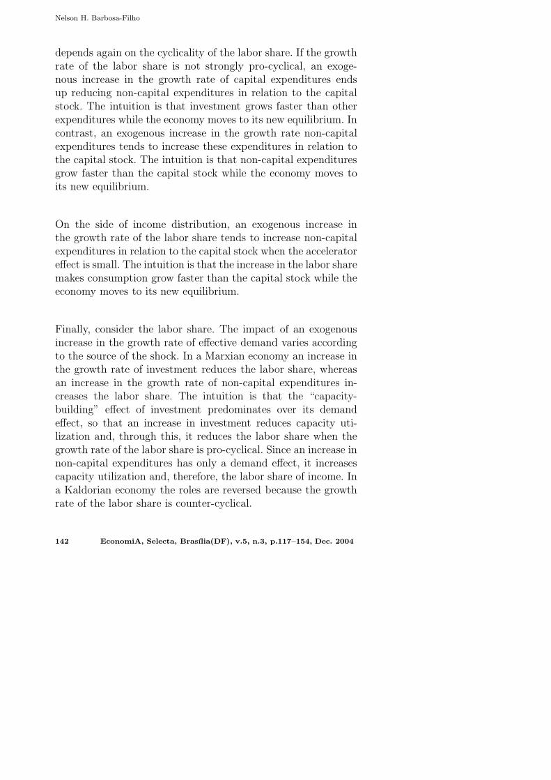
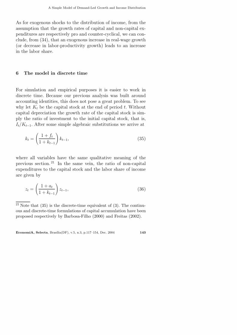
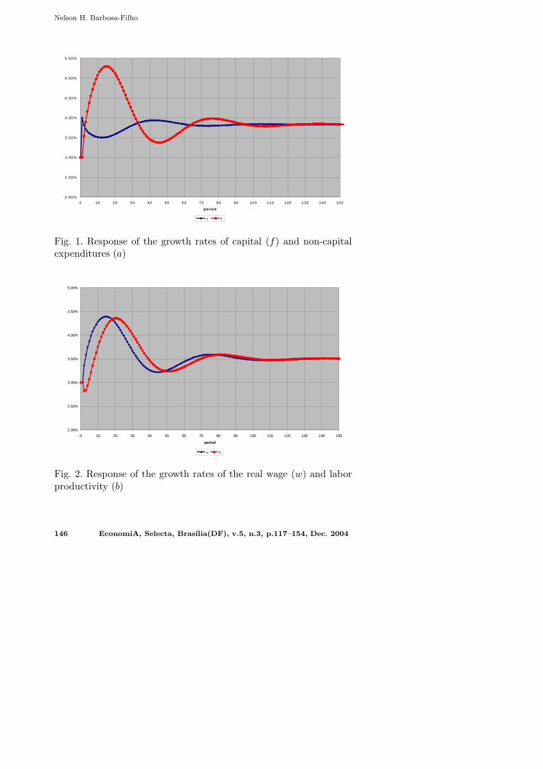
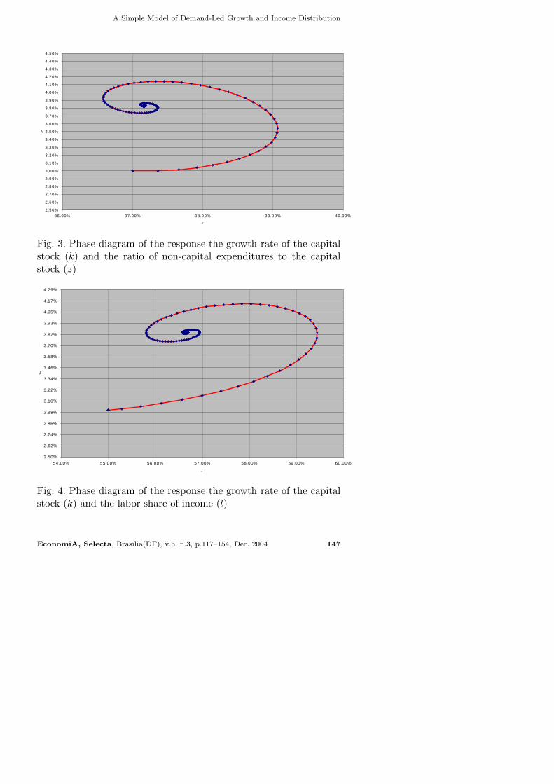
After substituting the above functions in (35), (36) and (37),we obtain a non-linear dynamical system in discrete time that,in principle, can be calibrated or estimated to reproduce thedynamics of real-world capitalist economies. To illustrate thispoint, figures 1 through 4 show the response of an artificial profit-led Marxian economy to an exogenous increase in the growth rateof autonomous expenditures. 22 The parameters of the modelwere chosen to obtain a steady state where the labor share ofincome is 0.55 and the income-capital ratio is 0.4, of which 0.03correspond to the growth rate of the capital stock and 0.37 tonon-capital expenditures. The implicit period is one year and,starting from the equilibrium point, the economy is subject to apermanent one-percentage point increase in the growth rate ofits non-capital expenditures. Figures 1 and 2 show the responseof the four behavioral functions to the shock, whereas figures 2and 3 show how the state variables move to their new equilibriumvalues.

22 Appendix 2 presents the values of the parameters used in the sim-ulation.



2.00%

2.50%

3.00%

3.50%

4.00%

4.50%

5.00%

5.50%

0 10 20 30 40 50 60 70 80 90 100 110 120 130 140 150

period

a f

Fig. 1. Response of the growth rates of capital (f) and non-capitalexpenditures (a)

2.00%

2.50%

3.00%

3.50%

4.00%

4.50%

5.00%

0 10 20 30 40 50 60 70 80 90 100 110 120 130 140 150

period

w b

Fig. 2. Response of the growth rates of the real wage (w) and laborproductivity (b)



2.5 0%

2.6 0%

2.7 0%

2.8 0%

2.9 0%

3.0 0%

3.1 0%

3.2 0%

3.3 0%

3.4 0%

3.5 0%

3.6 0%

3.7 0%

3.8 0%

3.9 0%

4.0 0%

4.1 0%

4.2 0%

4.3 0%

4.4 0%

4.5 0%

36 .00% 37 .00 % 3 8.0 0% 3 9.0 0% 40.00%

z

k

Fig. 3. Phase diagram of the response the growth rate of the capitalstock (k) and the ratio of non-capital expenditures to the capitalstock (z)

2.50%

2.62%

2.74%

2.86%

2.98%

3.10%

3.22%

3.34%

3.46%

3.58%

3.70%

3.82%

3.93%

4.05%

4.17%

4.29%

54.00% 55.00% 56.00% 57.00% 58.00% 59.00% 60.00%

l

k

Fig. 4. Phase diagram of the response the growth rate of the capitalstock (k) and the labor share of income (l)



On the demand side, the growth rate of non-capital expendituresslows down immediately after the shock and then it oscillateswhile converging to its new equilibrium value. In contrast, thegrowth rate of capital expenditures accelerates substantially af-ter the shock and then it also oscillates while converging to itsnew equilibrium value. On the income side, the growth rate of thereal wage accelerates after the shock and the growth rate of la-bor productivity follows it shortly after. Both variables oscillatewhile converging to their common and higher new equilibriumvalue. On the z×k plane the adjustment happens through coun-terclockwise fluctuations around the new equilibrium point. Onthe l × k plane the pattern is the same and, altogether, the ex-ogenous increase in the growth rate of non-capital expendituresdrives the economy to a new steady state with a faster growthrate, a higher income-capital ratio, and a higher labor share.

7 Conclusion

In general terms the main results of the previous sections can besummarized as follows:

• Income growth can be demand-led and stable under some plau-sible assumptions about aggregate demand, technology andincome distribution.

• Demand-led growth can be represented by a small dynamicalsystem in either continuous or discrete time. In both casesthe steady states and the dynamics around the steady statesdepends crucially on the intensity of the accelerator effect ofincome on investment; on the response of effective demand tochanges in income distribution; and on the response of incomedistribution to changes in effective demand.

• Demand-led growth may be stable under alternative assump-



tions about the cyclical behavior of the labor share (a profit-led or wage-led economy) or the response of effective demandto changes in income distribution (a Marxian or a Kaldorianeconomy).

• As long as the economy remains below its potential output,exogenous changes in effective demand may alter the growthrate and the functional distribution of income in both the shortand the long run. In other words, the economy may be lockedin a “slow-growth” or “fast-growth” steady state because ofdemand factors.

• Given a shock and assuming that demand-led growth and in-come distribution are jointly stable, the convergence to thesteady state may involve fluctuations of capacity utilizationand the labor share of income.

• Given the structure of the economy, the impact of exogenouschanges in effective demand on growth and distribution mayvary according to whether the source of the shock is a changein capital or non-capital expenditures.

Since we have many parameters in the behavioral functions thatdescribe effective demand, real wages and labor productivity, wehave a long list of possible results even in the linear case ana-lyzed in the previous sections. If we allow for nonlinear relationsthe list of possible results gets longer and the complexity muchhigher. Fortunately the linear behavioral functions already giveus a flexible starting point that can be adjusted to describe theevolution of real-world economies in terms of a historical analysisof waves of demand expansion.



References

Barbosa-Filho, N. H. (2000). A note on the theory of demand-ledgrowth. Contributions to Political Economy, 19.

Barbosa-Filho, N. H. (2001). Essays on Structuralist Macroeco-nomics. PhD thesis, New School for Social Research. Unpub-lished.

Barbosa-Filho, N. H. (2003). Effective demand and growth in aone-sector Keynesian model. In Salvadori, N., editor, Old andNew Growth Theories: An Assessment. Edward Elgar, Chel-tenham, U.K.

Barbosa-Filho, N. H. & Taylor, L. (2003). Distributive and de-mand cycles in the US economy – a structuralist goodwinmodel. Working paper 2003-03, New School for Social Re-search: Center for Economic Policy Analysis.

Blanchflower, D. G. & Oswald, A. J. (1995). The wage curve.Cambridge, MA: The MIT Press.

Commendatore, P., D’Acunto, S., Panico, C., & Pinto, A. (2003).Keynesian theories of growth. In Salvadori, N., editor, TheTheory of Economic Growth. Cletenham: Edward Elgar.

Dutt, A. (1990). Growth and uneven development. Cambridge,UK: Cambridge University Press.

Felipe, J. & Fisher, F. (2003). Aggregation in production func-tions: What applied economists should know. Metroeconomica,54:208–262.

Foley, D. & Marquetti, A. (1997). Economic growth from a clas-sical perspective. New School for Social Research, Departmentof Economics.

Foley, D. & Michl, T. (1999). Growth and distribution. Cam-bridge, MA: Harvard University Press.

Freitas, F. N. P. (2002). Uma Analise Da Evolucao Das Ideiasde Kaldor Sobre O Processo de Desenvolvimento Economico.PhD thesis, Institute of Economics, Federal University of Riode Janeiro. Unpublished.



Gandolfo, G. (1997). Economic dynamics. Berlin: Springer-Verlag.

Goodwin, R. M. (1967). A growth cycle. In Feinstein, C. H.,editor, Socialism, Capitalism, and Growth. Cambridge: Cam-bridge University Press.

Harrod, R. (1939). An essay in dynamic theory. Economic Jour-nal, 49:14–33.

Hicks, J. (1965). Capital and growth. Oxford: Clarendon.Kaldor, N. (1956). Alternative theories of distribution. Review

of Economic Studies, 23:83–100.Kalecki, M. (1971). Selected essays on the dynamics of the capi-

talist economy: 1933–70. Cambridge, UK: Cambridge Univer-sity Press.

Keynes, J. M. (1936). The general theory of employment, interestand Money. London: MacMillan.

Kurz, H. D. & Salvadori, N. (1995). A theory of production: Along-period analysis. Cambridge: Cambridge University Press.

Lavoie, M. (1992). Foundations of Post-Keynesian economicanalysis. Cheltenham: Edward Elgar.

Leon-Ledesma, M. & Thirlwall, A. P. (2000). Is the natural rateof growth exogenous. Banca Nazionale del Lavoro QuarterlyReview, 215:435–379–445.

Lewis, A. C. (1954). Economic development with unlimited sup-plies of labor. Manchester School of Economics and SocialStudies, 22:139–191.

Marglin, S. A. (1984). Growth and distribution. Cambridge,MA: Harvard University Press.

Marglin, S. A. & Bhaduri, A. (1990). Profit squeeze and Key-nesian theory. In Marglin, S. A. & Schor, J., editors, TheGolden Age of Capitalism: Reinterpreting the Postwar Expe-rience. Oxford: Clarendon.

Panico, C. (2003). Old and new growth theory: What role for ag-gregate demand. In Salvadori, N., editor, Old and New GrowthTheories, an Assessment. Cheltenham, UK: Edward Elgar.



Sen, A. (1963). Neo-classical and neo-keynesian theories of dis-tribution. Economic Record, 39:54–64.

Solow, R. (1997). Is there a core of practical macroeconomicsthat we should all believe in? American Economic Review,87(2):230–232.

Solow, R. (2000). The neoclassical theory of growth and distribu-tion. Banca Nazionale del Lavoro Quarterly Review, 215:358–381.

Taylor, L. (1979). Macro models for developing countries. NewYork: McGraw-Hill.

Taylor, L. (1991). Income distribution, inflation and growth:Lectures on structuralist macroeconomic theory. Cambridge,MA: the MIT Press.

Taylor, L. (2004). Reconstructing macroeconomics: Structuralistproposals and critiques of the mainstream. Cambridge, MA:Harvard University Press.



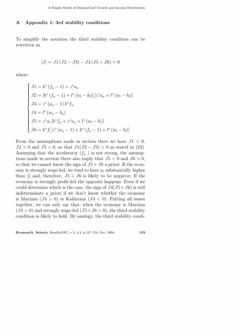
A Appendix 1: 3rd stability conditions

To simplify the notation the third stability condition can berewritten as

|J | = J1 (J2 − J3) − J4 (J5 + J6) < 0

where:

J1 = k∗ (fu − 1) + z∗au

J2 = [k∗ (fu − 1) + l∗ (wl − bl)] [z∗au + l∗ (wl − bl)]

J3 = z∗ (au − 1) k∗fu

J4 = l∗ (wu − bu)

J5 = z∗al [k∗fu + z∗au + l∗ (wl − bl)]

J6 = k∗fl [z∗ (au − 1) + k∗ (fu − 1) + l∗ (wl − bl)]

From the assumptions made in section three we have J1 < 0,J2 > 0 and J3 < 0, so that J1(J2 − J3) < 0 as stated in (23).Assuming that the accelerator (fu ) is not strong, the assump-tions made in section three also imply that J5 < 0 and J6 > 0,so that we cannot know the sign of J5+J6 a priori. If the econ-omy is strongly wage-led, we tend to have al substantially higherthan fl and, therefore, J5 + J6 is likely to be negative. If theeconomy is strongly profit-led the opposite happens. Even if wecould determine which is the case, the sign of J4(J5+J6) is stillindeterminate a priori if we don’t know whether the economyis Marxian (J4 > 0) or Kaldorian (J4 < 0). Putting all issuestogether, we can only say that, when the economy is Marxian(J4 > 0) and strongly wage-led (J5+J6 > 0), the third stabilitycondition is likely to hold. By analogy, the third stability condi-



tion is also likely to hold if the economy is Kaldorian (J4 < 0)and strongly profit-led (J5 + J6 < 0).

B Appendix 2: simulation

The values of the intercept coefficients were chosen to obtainan equilibrium point where k∗ = f ∗ = a∗ = w∗ = b∗ = 0.03,z∗ = 0.37, and l∗ = 0.55. The shock consists of a permanent0.01 increase in the intercept coefficient of the “a” function. Thesimulation used the following values for the parameters of thebehavioral functions:

Intercept z k l

a 0.120 -0.5 -0.5 0.2

f -0.350 1.5 1.5 -0.4

w -0.205 1 1 -0.3

b -0.100 -0.5 -0.5 0.6


a simple model of demand-led growth and income...

Documents