a short course in combinatorial designs · 1.3 optimal assignment problem ... s3 = fa;dg;s4 =...

A Short Course inCombinatorial Designs

Ian AndersonDepartment of Mathematics

University of GlasgowGlasgow G12 8QW, UK

e-mail: [email protected]

Iiro HonkalaDepartment of Mathematics

University of Turku20014 Turku, Finlande-mail: [email protected]

Copyright Notice

Copyright 1997 by Ian Anderson and Iiro Honkala. This material may bereproduced for any educational purpose, multiple copies may be made forclasses, etc. Charges, if any, for reproduced copies must be just enough to re-cover reasonable costs of reproduction. Reproduction for commercial purposesis prohibited. This cover page must be included in all distributed copies.

Internet Edition, Spring 1997, Revised 2012

Contents

1 Systems of distinct representatives 11.1 Hall’s theorem . . . . . . . . . . . . . . . . . . . . . . . . . . . 11.2 Latin squares . . . . . . . . . . . . . . . . . . . . . . . . . . . . 21.3 Optimal assignment problem . . . . . . . . . . . . . . . . . . . 3

2 2-designs 72.1 Definition and basic properties of (v, k, λ) designs . . . . . . . . 72.2 Resolvable designs . . . . . . . . . . . . . . . . . . . . . . . . . 92.3 Incidence matrix of a design . . . . . . . . . . . . . . . . . . . . 92.4 Symmetric designs . . . . . . . . . . . . . . . . . . . . . . . . . 112.5 Hadamard matrices and designs . . . . . . . . . . . . . . . . . . 132.6 Finite projective planes . . . . . . . . . . . . . . . . . . . . . . 152.7 Lagrange’s theorem . . . . . . . . . . . . . . . . . . . . . . . . . 182.8 The theorem of Bruck, Ryser and Chowla . . . . . . . . . . . . 202.9 Mutually orthogonal Latin squares . . . . . . . . . . . . . . . . 242.10 Difference sets . . . . . . . . . . . . . . . . . . . . . . . . . . . . 27

3 t-designs and Steiner systems 293.1 Basic definitions and properties . . . . . . . . . . . . . . . . . . 293.2 Steiner triple systems . . . . . . . . . . . . . . . . . . . . . . . 32

4 Codes and designs 334.1 Basics on codes . . . . . . . . . . . . . . . . . . . . . . . . . . . 334.2 The binary Golay code . . . . . . . . . . . . . . . . . . . . . . . 354.3 Steiner systems S(5, 8, 24) and S(5, 6, 12) . . . . . . . . . . . . 37

Bibliography 39

Chapter 1

Systems of distinctrepresentatives

1.1 Hall’s theorem

Example 1.1 Assume that there are five vacant jobs 1, 2, 3, 4 and 5. Denoteby Si the set of applicants for the job i. If we assume that

S1 = {A,B, C}, S2 = {D, E}, S3 = {A,D}, S4 = {E}, S5 = {A,E},is it possible to assign a different person to each job? Clearly, in this specificcase the answer is no. Indeed, we must assign E to 4, D to 2, A to 3 andthere is nobody left for the job 5. ¤

Consider the general case.

Definition 1.2 A system of distinct representatives for the sets S1, S2, . . . ,Sn is an n-tuple (x1, x2, ..., xn) where the elements xi are distinct and xi ∈ Si

for all i = 1, 2, . . . , n.

In the previous example the sets Si did not have a system of distinctrepresentatives for the following very simple reason: the union of certain foursets had fewer than four elements. Clearly, if the sets S1, S2, . . . , Sn have asystem of distinct representatives, then the union of any k (1 ≤ k ≤ n) setshas at least k elements. Surprisingly, this obvious necessary condition is alsosufficient.

Theorem 1.3 (Philip Hall) The sets S1, S2, . . . , Sn have a system of distinctrepresentatives if and only if

for every k = 1, 2, ..., n the union of any k sets has at least k elements.

1

2 Chapter 1. Systems of distinct representatives

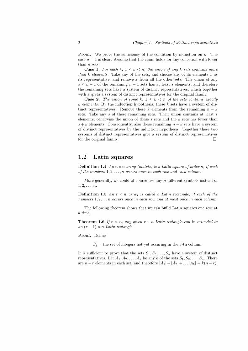
Proof. We prove the sufficiency of the condition by induction on n. Thecase n = 1 is clear. Assume that the claim holds for any collection with fewerthan n sets.

Case 1: For each k, 1 ≤ k < n, the union of any k sets contains morethan k elements. Take any of the sets, and choose any of its elements x asits representative, and remove x from all the other sets. The union of anys ≤ n − 1 of the remaining n − 1 sets has at least s elements, and thereforethe remaining sets have a system of distinct representatives, which togetherwith x gives a system of distinct representatives for the original family.

Case 2: The union of some k, 1 ≤ k < n of the sets contains exactlyk elements. By the induction hypothesis, these k sets have a system of dis-tinct representatives. Remove these k elements from the remaining n − ksets. Take any s of these remaining sets. Their union contains at least selements; otherwise the union of these s sets and the k sets has fewer thans + k elements. Consequently, also these remaining n− k sets have a systemof distinct representatives by the induction hypothesis. Together these twosystems of distinct representatives give a system of distinct representativesfor the original family. ¤

1.2 Latin squares

Definition 1.4 An n×n array (matrix) is a Latin square of order n, if eachof the numbers 1, 2, . . . , n occurs once in each row and each column.

More generally, we could of course use any n different symbols instead of1, 2, . . . , n.

Definition 1.5 An r × n array is called a Latin rectangle, if each of thenumbers 1, 2, . . . n occurs once in each row and at most once in each column.

The following theorem shows that we can build Latin squares one row ata time.

Theorem 1.6 If r < n, any given r × n Latin rectangle can be extended toan (r + 1)× n Latin rectangle.

Proof. Define

Sj = the set of integers not yet occuring in the j-th column.

It is sufficient to prove that the sets S1, S2, . . . , Sn have a system of distinctrepresentatives. Let A1, A2, . . . , Ak be any k of the sets S1, S2, . . . , Sn. Thereare n− r elements in each set, and therefore |A1|+ |A2|+ . . . |Ak| = k(n− r).

1.3. Optimal assignment problem 3

Each number occurs once in each of the r rows and hence in n− r of the setsSi, and consequently in at most n−r of the sets Ai. Therefore |A1∪. . .∪Ak| ≥k(n− r)/(n− r) = k. The claim now follows from Hall’s theorem. ¤

1.3 Optimal assignment problem

In Example 1.1 we did not pay any attention to how suitable the individualapplicants were to each job.

Example 1.7 Four persons a1, a2, a3 and a4 should be assigned to the jobsJ1, J2, J3 and J4, and the left-hand side table below gives the available infor-mation about their suitability:

J1 J2 J3 J4

a1 11 9 1 4a2 8 13 7 6a3 12 2 14 11a4 10 13 15 2

,

J1 J2 J3 J4

a1 −11 −9 −1 −4a2 −8 −13 −7 −6a3 −12 −2 −14 −11a4 −10 −13 −15 −2

.

Our goal is to choose four entries, no two in the same row or column, in sucha way that the sum of the entries is maximized. For practical reasons weinstead consider the unsuitability of the applicants and try to minimize thesum of the unsuitability numbers. We do this by changing the signs of all theentries, which gives the right-hand side table above. Since we choose exactlyone entry from each row and column, it is clear that if the same integer isadded to (or subtracted from) all the entries in a row or column, the optimalchoices still remain the same — although the sum of the corresponding entriesof course changes. In this example we can therefore add 11 to all the entriesof the first row and 13, 14 and 15 to the entries of the second, third andfourth rows, respectively, and finally subtract 3 from all the entries in the lastcolumn to obtain the table

J1 J2 J3 J4

a1 0 2 10 4a2 5 0 6 4a3 2 12 0 0a4 5 2 0 10

.

Notice that we made all the entries nonnegative. Consequently, if we can findfour 0’s, no two in the same row or column, they correspond to an optimalassignment. In this example this is possible in a unique way: the uniqueoptimal assignment is to choose a1 to J1, a2 to J2, a3 to J4 and a4 to J3. ¤


We were lucky in the previous example, because we immediately foundfour suitable zeroes. In general, we need one more trick.

Theorem 1.8 Let A be an m × n matrix. The maximum number of inde-pendent zeros, i.e., zeros no two in the same row or column, is equal to theminimum number of rows and columns required to cover all the zeros in A.

Proof. Denote by α the maximum number of independent zeros and by β theminimum number of rows or columns required to cover all the zeros. Clearly,β ≥ α, because we can find α independent zeros in A, and any row or columncovers at most one of them.

We need to prove that α ≥ β. Assume that some a rows and b columnscover all the zeros and a + b = β. Because permuting the rows and columnschanges neither α nor β, we may assume that the first a rows and the first bcolumns cover the zeros. Write A in the form

A =(

Ca×b Da×(n−b)

E(m−a)×b F(m−a)×(n−b)

). (1.9)

We know that there are no zeros in F. We show that there are a indepen-dent zeros in D. The same argument shows — by symmetry — that thereare b independent zeros in E. Together these a + b zeros, which are clearlyindependent, show that α ≥ a + b = β.

We use Hall’s theorem. Define

Si = {j | dij = 0} ⊆ {1, 2, . . . , n− b},

the set of locations of the zeros in the i-th row of D = (dij). We claim thatthe family S1, S2, . . . , Sa has a system of distinct representatives, i.e., wecan choose one zero from each row, no two in the same column. Otherwise,Hall’s theorem tells us that the union of some k of these sets has fewer thank elements, which means that the zeros in these rows can all covered by somes < k columns. But then we obtain a covering of all the zeros in A whichcontains fewer than a + b rows and columns, a contradiction. ¤

Consider now the general optimal assignment problem. Assume that npersons a1, a2, . . . , an are to be assigned to n jobs J1, J2, . . . , Jn and thatwe have an n × n matrix with integer entries representing the suitability ofthe applicants to the jobs. In the same way as in Example 1.7 we get to asituation where we have an n× n matrix A with nonnegative integer entriesrepresenting the unsuitability of the applicants, and there is already at leastone zero in each row and column.

If there are n independent zeros in A, the problem has been solved: eachsuch set of n independent zeros gives an optimal assignment, and there are

1.3. Optimal assignment problem 5

no others. Assume that the maximum number of independent zeros in A isr < n. By the previous theorem there are nonnegative integers a and b witha + b = r such that all the zeros in A can be covered by some a rows and bcolumns. If they are again the first a rows and b columns and A is as in (1.9),then denote by s the smallest of the numbers in F. We now add s to all thesea rows (i.e., to the entries in C and D) and subtract s from all except thefirst b columns (i.e., from the entries in D and F). The net effect is that allthe entries in C have increased by s and all the entries in F have decreasedby s and all the other entries remained unchanged. Consequently, the sum ofall the entries in the matrix has decreased by the quantity

(n− a)(n− b)s− abs = n(n− a− b)s > 0,

because a + b = r < n. All the entries in the resulting matrix A′ are stillnonnegative integers. If A′ still does not contain n independent zeros, weapply the same trick again. Eventually the process has to terminate, becausethe sum of all the entries in the matrix decreases in each step and can neverbecome negative.

Example 1.10 Assume that in an optimal assignment problem for four per-sons and four jobs the unsuitability matrix is

6 8 2 75 8 13 92 7 8 94 11 7 10

.

By subtracting the smallest entry from each row and then the smallest entryfrom each column, we obtain the matrices

4 6 0 50 3 8 40 5 6 70 7 3 6

4 3 0 10 0 8 00 2 6 30 4 3 2

.

All the zeros are covered by the first two rows and the first column, so thereare no four independent zeros. The smallest entry in the lower right-handblock is 2, so we subtract 2 from each element in this block, and add 2 to thetwo entries in the upper left-hand block to obtain

6 3 0 12 0 8 00 0 4 10 2 1 0

.


Now we can find four independent zeros. In fact we see that there are exactlytwo different optimal assignments. In both cases the sum of the unsuitabilitynumbers (in the original matrix) is 22 — in the resulting matrix it is of course0. ¤

Notice that the same technique can also be used even if there are morejobs than applicants: we can add dummy extra applicants who are equallysuited for all the jobs.

Chapter 2

2-designs

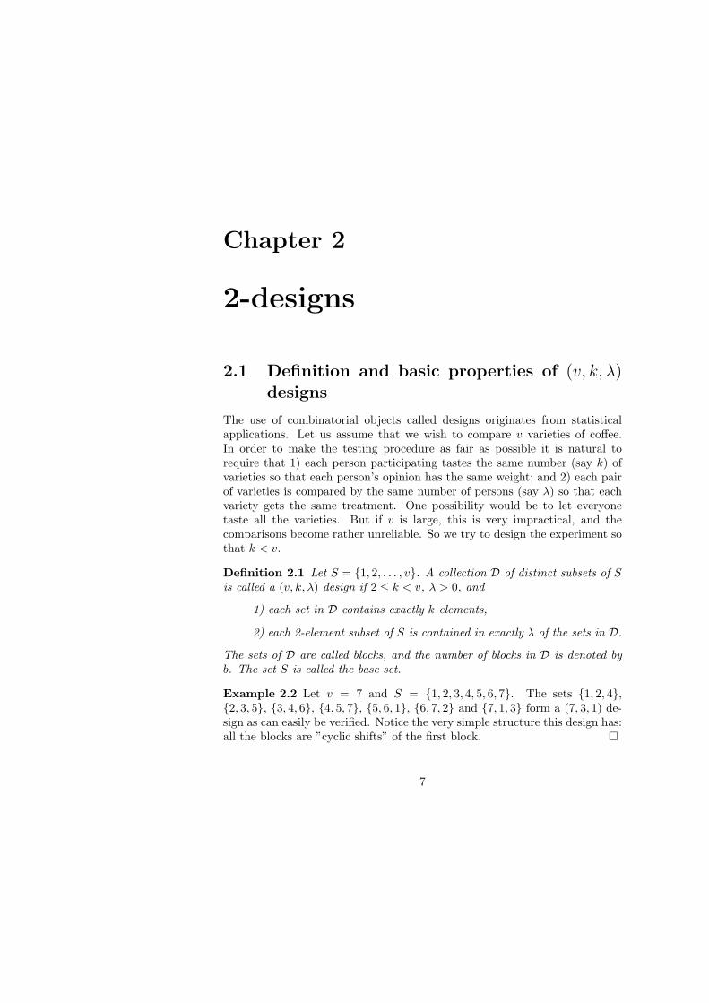
2.1 Definition and basic properties of (v, k, λ)designs

The use of combinatorial objects called designs originates from statisticalapplications. Let us assume that we wish to compare v varieties of coffee.In order to make the testing procedure as fair as possible it is natural torequire that 1) each person participating tastes the same number (say k) ofvarieties so that each person’s opinion has the same weight; and 2) each pairof varieties is compared by the same number of persons (say λ) so that eachvariety gets the same treatment. One possibility would be to let everyonetaste all the varieties. But if v is large, this is very impractical, and thecomparisons become rather unreliable. So we try to design the experiment sothat k < v.

Definition 2.1 Let S = {1, 2, . . . , v}. A collection D of distinct subsets of Sis called a (v, k, λ) design if 2 ≤ k < v, λ > 0, and

1) each set in D contains exactly k elements,

2) each 2-element subset of S is contained in exactly λ of the sets in D.

The sets of D are called blocks, and the number of blocks in D is denoted byb. The set S is called the base set.

Example 2.2 Let v = 7 and S = {1, 2, 3, 4, 5, 6, 7}. The sets {1, 2, 4},{2, 3, 5}, {3, 4, 6}, {4, 5, 7}, {5, 6, 1}, {6, 7, 2} and {7, 1, 3} form a (7, 3, 1) de-sign as can easily be verified. Notice the very simple structure this design has:all the blocks are ”cyclic shifts” of the first block. ¤

7

8 Chapter 2. 2-designs

Theorem 2.3 If D is a (v, k, λ) design, then each element of the base setoccurs in r blocks, where

r(k − 1) = λ(v − 1). (2.4)

Moreover,bk = vr. (2.5)

Proof. Let a ∈ S be fixed and assume that a occurs in ra blocks. We countin two ways the cardinality of the set

{(x,B) | B ∈ D, a, x ∈ B, a 6= x}.For each of the v − 1 possibilities for x (x 6= a) there are exactly λ blocksB containing both a and x. The cardinality of the set is therefore (v − 1)λ.On the other hand, for each of the ra blocks B containing a, the element xcan be chosen to be any of the k − 1 elements in B other than a. Hence(v−1)λ = ra(k−1). This shows that ra is independent of the choice of a andproves (2.4).

To prove the second claim we count in two ways the cardinality of the set

{(x,B) | B ∈ D, x ∈ B}.For each x ∈ S the block B can be chosen in r ways; on the other hand, foreach of the b blocks B the element x ∈ B can be chosen in k ways. Hencevr = bk. ¤

Theorem 2.3 shows that the five parameters v, k, λ, b, r are not independentof each other: we can determine b and r from v, k and λ.

A basic question in design theory is to determine for which values of v, kand λ there is a (v, k, λ) design. Certainly, such designs do not exist for allv, k and λ, already by Theorem 2.3.

Example 2.6 There is no (11, 6, 2) design. Otherwise, Theorem 2.3 impliesthat r = 4 and 6b = 44, a contradiction. ¤

Theorem 2.7 If D is a (v, k, λ) design, then its complement D defined by

D = {S \B | B ∈ D}is a (v, v − k, b− 2r + λ) design provided that b− 2r + λ > 0.

Proof. Clearly every block of D has v− k elements. Moreover, a pair (x, y),x, y ∈ S, x 6= y, is contained in S \ B if and only if B contains neither x nory. The number of blocks of D containing neither x nor y is b− 2r + λ by theprinciple of inclusion and exclusion. ¤

2.2. Resolvable designs 9

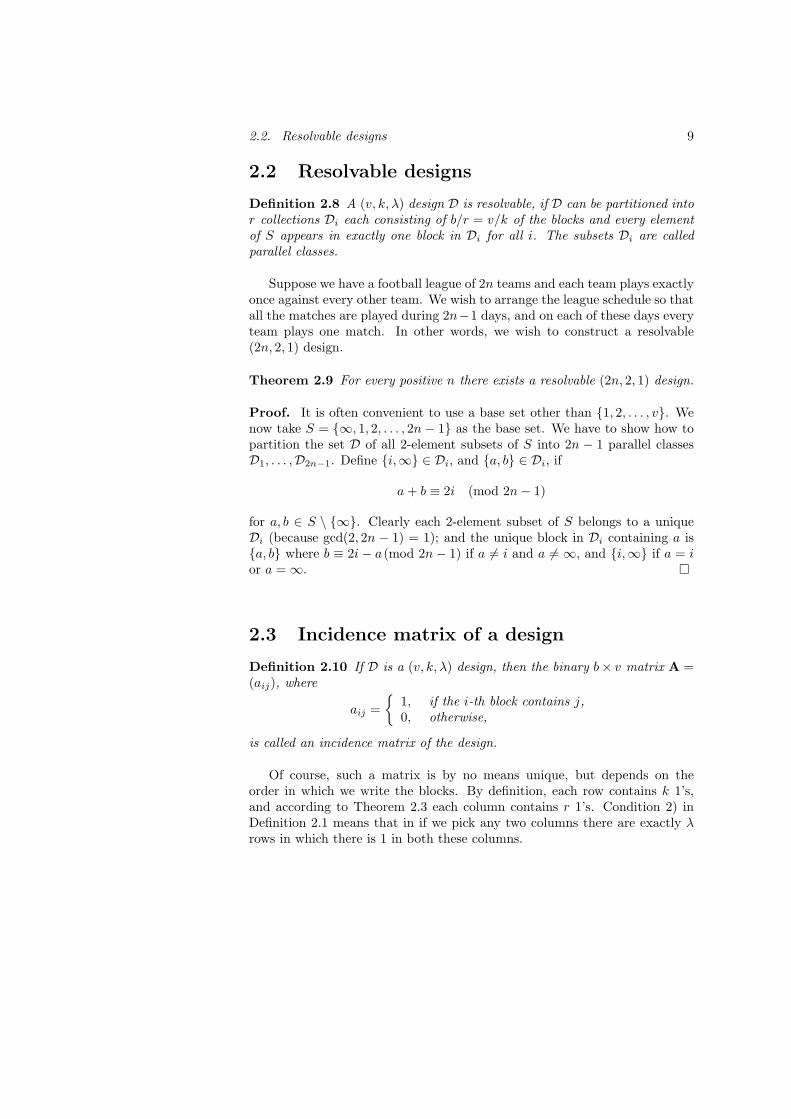
2.2 Resolvable designs

Definition 2.8 A (v, k, λ) design D is resolvable, if D can be partitioned intor collections Di each consisting of b/r = v/k of the blocks and every elementof S appears in exactly one block in Di for all i. The subsets Di are calledparallel classes.

Suppose we have a football league of 2n teams and each team plays exactlyonce against every other team. We wish to arrange the league schedule so thatall the matches are played during 2n−1 days, and on each of these days everyteam plays one match. In other words, we wish to construct a resolvable(2n, 2, 1) design.

Theorem 2.9 For every positive n there exists a resolvable (2n, 2, 1) design.

Proof. It is often convenient to use a base set other than {1, 2, . . . , v}. Wenow take S = {∞, 1, 2, . . . , 2n− 1} as the base set. We have to show how topartition the set D of all 2-element subsets of S into 2n − 1 parallel classesD1, . . . ,D2n−1. Define {i,∞} ∈ Di, and {a, b} ∈ Di, if

a + b ≡ 2i (mod 2n− 1)

for a, b ∈ S \ {∞}. Clearly each 2-element subset of S belongs to a uniqueDi (because gcd(2, 2n − 1) = 1); and the unique block in Di containing a is{a, b} where b ≡ 2i− a(mod 2n− 1) if a 6= i and a 6= ∞, and {i,∞} if a = ior a = ∞. ¤

2.3 Incidence matrix of a design

Definition 2.10 If D is a (v, k, λ) design, then the binary b× v matrix A =(aij), where

aij ={

1, if the i-th block contains j,0, otherwise,

is called an incidence matrix of the design.

Of course, such a matrix is by no means unique, but depends on theorder in which we write the blocks. By definition, each row contains k 1’s,and according to Theorem 2.3 each column contains r 1’s. Condition 2) inDefinition 2.1 means that in if we pick any two columns there are exactly λrows in which there is 1 in both these columns.


Theorem 2.11 If A is an incidence matrix of a (v, k, λ) design, then

AT A = (r − λ)I + λJ,

where I is the v × v identity matrix and J the v × v matrix in which everyentry is 1.

Proof. Clearly AT A is a v × v matrix whose (i, j) entry is the real innerproduct of the i-th and j-th columns of A. If i = j, this is just the numberof 1’s in this column, i.e., equal to r. If i 6= j, then it is the number of rowsin which both the i-th and j-th column have 1, i.e., it equals λ. ¤

Theorem 2.12 (Fisher’s inequality) If there is a (v, k, λ) design, then b ≥ v.

Proof. Let A be an incidence matrix of a (v, k, λ) design, and consider thedeterminant of AT A, the matrix we calculated in the previous theorem. Bysubtracting the first row from the others we obtain

det(AT A) =

∣∣∣∣∣∣∣∣∣∣∣

r λ λ . . . λλ r λ . . . λλ λ r . . . λ...

...λ λ λ . . . r

∣∣∣∣∣∣∣∣∣∣∣

=

∣∣∣∣∣∣∣∣∣∣∣

r λ λ . . . λλ− r r − λ 0 . . . 0λ− r 0 r − λ . . . 0

......

λ− r 0 0 . . . r − λ

∣∣∣∣∣∣∣∣∣∣∣

.

By adding the other columns to the first one we obtain

det(AT A) =

∣∣∣∣∣∣∣∣∣∣∣

r + (v − 1)λ λ λ . . . λ0 r − λ 0 . . . 00 0 r − λ . . . 0...

...0 0 0 . . . r − λ

∣∣∣∣∣∣∣∣∣∣∣= (r + (v − 1)λ)(r − λ)v−1

= rk(r − λ)v−1

by (2.4), which also implies that r > λ, because we have assumed k < v.Therefore det(AT A) 6= 0.

Assume now on the contrary that b < v. Then there are fewer rows thancolumns in A. We add v − b rows of zeros to A to obtain a v × v matrix A1.Clearly AT

1 A1 = AT A, because adding zeros has no effect on the real innerproducts of the columns. But since A1 is a square matrix, the product rulefor determinants implies that

det(AT A) = det(AT1 A1) = det(AT

1 ) det(A1) = 0,

because there is at least one row of zeros in A1. ¤

2.4. Symmetric designs 11

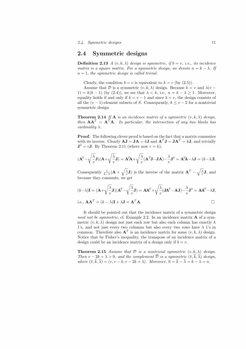
2.4 Symmetric designs

Definition 2.13 A (v, k, λ) design is symmetric, if b = v, i.e., its incidencematrix is a square matrix. For a symmetric design, we denote n = k − λ. Ifn = 1, the symmetric design is called trivial.

Clearly, the condition b = v is equivalent to k = r (by (2.5)).Assume that D is a symmetric (v, k, λ) design. Because k < v and λ(v −

1) = k(k − 1) (by (2.4)), we see that λ < k, i.e., n = k − λ ≥ 1. Moreover,equality holds if and only if k = v − 1 and since b = v, the design consists ofall the (v − 1)-element subsets of S. Consequently, k ≤ v − 2 for a nontrivialsymmetric design.

Theorem 2.14 If A is an incidence matrix of a symmetric (v, k, λ) design,then AAT = AT A. In particular, the intersection of any two blocks hascardinality λ.

Proof. The following clever proof is based on the fact that a matrix commuteswith its inverse. Clearly AJ = JA = kJ and AT J = JAT = kJ, and triviallyJ2 = vJ. By Theorem 2.11 (where now r = k),

(AT−√

λ

vJ)(A+

√λ

vJ) = ATA+

√λ

v(ATJ−JA)−λ

vJ2 = ATA−λJ = (k−λ)I.

Consequently 1k−λ (A +

√λv J) is the inverse of the matrix AT −

√λv J, and

because they commute, we get

(k−λ)I = (A+

√λ

vJ)(AT−

√λ

vJ) = AAT +

√λ

v(JAT−AJ)−λ

vJ2 = AAT−λJ,

i.e., AAT = (k − λ)I + λJ = AT A. ¤

It should be pointed out that the incidence matrix of a symmetric designneed not be symmetric, cf. Example 2.2. In an incidence matrix A of a sym-metric (v, k, λ) design not just each row but also each column has exactly k1’s, and not just every two columns but also every two rows have λ 1’s incommon. Therefore also AT is an incidence matrix for some (v, k, λ) design.Notice that by Fisher’s inequality, the transpose of an incidence matrix of adesign could be an incidence matrix of a design only if b = v.

Theorem 2.15 Assume that D is a nontrivial symmetric (v, k, λ) design.Then v − 2k + λ > 0, and the complement D is a symmetric (v, k, λ) design,where (v, k, λ) = (v, v − k, v − 2k + λ). Moreover, n = k − λ = k − λ = n.


Proof. By the discussion preceding the proof k ≤ v− 2. Let B be any blockand {x, y} ⊆ S \ B, x 6= y. By the proof of Theorem 2.7, v − 2k + λ is thenumber of blocks of D containing neither x nor y, and hence positive. Theresult now follows from Theorem 2.7. ¤

Theorem 2.16 If a nontrivial symmetric (v, k, λ) design exists, then

4n− 1 ≤ v ≤ n2 + n + 1.

Proof. Using the notations of Theorem 2.15, λ + λ = v − 2n and

λλ = λ(v − 2k + λ) = λ(v − 1) + λ− 2λk + λ2 = k(k − 1) + λ− 2λk + λ2

= (k − λ)2 − (k − λ) = n(n− 1).

For all real numbers x and y, (x + y)2 ≥ 4xy. Hence for x = λ and y = λ,(v − 2n)2 ≥ 4n(n− 1) > (2n− 2)2 because n ≥ 2, and therefore (v − 2n)2 ≥(2n− 1)2. Furthermore v − 2n = λ + λ > 0, and hence v − 2n ≥ 2n− 1, i.e.,v ≥ 4n− 1.

Because λ ≥ 1 and λ ≥ 1,

0 ≤ (λ− 1)(λ− 1) = λλ− (λ + λ) + 1 = n(n− 1)− (v − 2n) + 1,

i.e., v ≤ n2 + n + 1. ¤

Consider now the extreme cases.

Theorem 2.17 If D is a nontrivial symmetric (v, k, λ) design with v = n2 +n + 1, then D or D is a (n2 + n + 1, n + 1, 1) design.

Proof. From the proof of Theorem 2.16 we see that v = n2 + n + 1 impliesthat λ = 1 or λ = 1. If λ = 1, then k = n + λ = n + 1, and hence D is a(n2 + n + 1, n + 1, 1) design. If λ = 1, then k = n + λ = n + 1 = n + 1 byTheorem 2.15, and hence D is a (n2 + n + 1, n + 1, 1) design. ¤

Definition 2.18 An (n2 + n + 1, n + 1, 1) design (which is automaticallysymmetric) is called a (finite) projective plane of order n.

In fact, the finite projective planes are the only symmetric designs withλ = 1. Indeed, if λ = 1, then k = n + λ = n + 1, and v − 1 = λ(v − 1) =k(k − 1) = (n + 1)n, i.e., v = n2 + n + 1.

Theorem 2.19 If D is a nontrivial symmetric (v, k, λ) design with v = 4n−1,then D or D is a (4n− 1, 2n− 1, n− 1) design.

2.5. Hadamard matrices and designs 13

Proof. From the proof of Theorem 2.16 we see that λλ = n(n − 1) andλ+λ = v−2n = 2n−1. Thus λ and λ are the roots of the quadratic equationx2 − (2n− 1)x + n(n− 1) = 0, i.e., they are n and n− 1. If λ = n− 1, thenk = n + λ = 2n − 1, and D is a (4n − 1, 2n − 1, n − 1) design. If λ = n − 1,then k = n + λ = n + λ = 2n− 1, and D is a (4n− 1, 2n− 1, n− 1) design. ¤

Definition 2.20 A (4n − 1, 2n − 1, n − 1) design (which is automaticallysymmetric) is called a Hadamard design of order n.

2.5 Hadamard matrices and designs

Definition 2.21 An m ×m (m ≥ 2) matrix H whose entries belong to theset {−1, 1} is called a Hadamard matrix of order m if HT H = mI.

Example 2.22 We clearly obtain an infinite family of Hadamard matricesby defining

H2 =(

1 11 −1

),H2m =

(Hm Hm

Hm −Hm

)

for m = 2, 4, 8, . . ..

If we know that all the entries in H belong to the set {−1, 1}, then theequation HT H = mI is equivalent to saying that the columns of H are or-thogonal (i.e., their real inner product is 0).

Let H be an m × m matrix. If HT H = mI, then HHT = mI; andconversely. Indeed, in either case we see that H has an inverse and H−1 =1mHT , and the matrix and its inverse commute. For a matrix H whose entriesbelong to the set {−1, 1}, the equation HHT = mI is equivalent to sayingthat the rows of H are orthogonal.

Theorem 2.23 An m ×m matrix whose elements belong to the set {−1, 1}is a Hadamard matrix if and only if its columns (rows) are orthogonal. ¤

We can therefore multiply any rows and columns by −1 to obtain otherHadamard matrices. A Hadamard matrix is normalized if its first row andcolumn consist entirely of 1’s.

Theorem 2.24 If H is a Hadamard matrix of order m and its first row(column) consists entirely of 1’s, then every other row (column) has m/2 1’sand m/2 −1’s. If m > 2, then any two rows (columns) other than the firstrow (column) have exactly m/4 1’s in common.


Proof. The first statement immediately follows from the fact that the innerproduct of any row with the first row is 0.

Let R and S be two rows other than the first, and u (resp. v) the numberof places where they both have 1’s (resp. −1’s). Because R has m/2 1’s andm/2 −1’s we get the figure

First row 1 1 . . . 1 1 1 . . . 1 1 1 . . . 1 1 1 . . . 1R 1 1 . . . 1 1 1 . . . 1 −1−1 . . .−1 −1−1 . . .−1S 1 1 . . . 1 −1−1 . . .−1 1 1 . . . 1 −1−1 . . .−1

u m/2− u m/2− v v

.

Because S has m/2 1’s, the third quantity m/2−v has to be equal to m/2−u,i.e., u = v. The orthogonality of R and S then implies u−(m/2−u)−(m/2−u) + u = 0, i.e., u = m/4.

The claim for columns immediately follows by applying the result for rowsto the the Hadamard matrix HT . ¤

Corollary 2.25 If there is a Hadamard matrix of order m, then m = 2 orm is divisible by 4. ¤

It is conjectured that Hadamard matrices exist for all orders that aredivisible by 4.

Theorem 2.26 If n ≥ 2, there exists a Hadamard matrix of order 4n if andonly if there exists a Hadamard design of order n, i.e., a (4n−1, 2n−1, n−1)design.

Proof. Assume first that there exists a Hadamard matrix of order 4n, and letH be a normalized Hadamard matrix of order 4n. Form a (4n− 1)× (4n− 1)matrix A by deleting the first row and column in H and changing −1’s to0’s. This is an incidence matrix of a (4n− 1, 2n− 1, n− 1) design, because byTheorem 2.24 each row of A has 2n − 1 1’s and any two columns of A haveexactly n− 1 1’s in common.

Conversely, assume that there exists a (4n− 1, 2n− 1, n− 1) design, andlet A be its incidence matrix. Form a matrix H by changing the 0’s in A to−1’s and adding a further row and column of 1’s. Consider the inner productof the i-th and j-th columns (1 < i < j). The number of positions in whichthey both have 1 equals 1 + λ = 1 + (n − 1) = n. Since there are 2n 1’s ineach column, there are n positions where the i-th column has 1 and the j-thcolumn has −1 and similarly n positions where the i-th column has −1 andthe j-th column has 1. All in all, their inner product is n − n − n + n = 0.Therefore H is a Hadamard matrix by Theorem 2.23. ¤

2.6. Finite projective planes 15

Let H be a Hadamard matrix of order m. Take all the rows of the matricesH and −H, and change all −1’s to 0. In this way we obtain a set of 2m binaryvectors of length m called the Hadamard code Bm.

Theorem 2.27 Every two codewords in Bm differ in at least m/2 coordinates.

Proof. Take any a,b ∈ Bm, a 6= b. If a and b have been obtained fromthe i-th rows of H and −H respectively, then a disagrees with b in all mcoordinates. Otherwise for some two different rows x and y of H, the word ais obtained (by changing −1’s to 0’s) from x or −x, and b from y or −y. Inall cases, a and b differ in m/2 coordinates, because x and y are orthogonal,x and −y are orthogonal, −x and y are orthogonal, and −x and −y areorthogonal. ¤

2.6 Finite projective planes

Recall that a commutative ring (F, +, ·) where each nonzero element a hasa multiplicative inverse a−1 is called a field. For instance, if p is a prime,the set of residue classes ZZp modulo p with respect to usual addition andmultiplication is a field. From algebra we assume the following result.

Theorem 2.28 For every prime power q there exists a finite field IFq of qelements.

In the definition of a (v, k, λ) design we have used S = {1, 2, . . . , v} as thebase set. The choice of the base set is of course irrelevant, and we can chooseany set of v distinct elements just as well.

Denote by V the set of all vectors x = (x0, x1, x2) of elements in IFq wherex0, x1, x2 are not all zero. We identify the vectors that can obtained fromeach other by multiplying by an element in IF∗q = IFq \ {0}. More formally,we define an equivalence relation ∼ in the set V by the condition

x ∼ y if x = λy for some λ ∈ IF∗q .

Clearly, this is an equivalence relation. We denote the equivalence class con-taining x by [x], and the set of all equivalence classes by S.

Example 2.29 Take q = 3; then IF3 = ZZ3, and we denote the three ele-ments in IF3 by 0,1 and 2. The set V consists of all the 26 nonzero vectors(0, 0, 1), (0, 0, 2), (0, 1, 0), (0, 1, 1), (0, 1, 2) . . . , (2, 2, 2). Now IF∗q = {1, 2}, sowe identify two vectors x and y if x = y or x = 2y. Consequently, eachvector is identified with exactly one other vector and the set S consists of the13 equivalence classes


[(0, 0, 1)] = [(0, 0, 2)] = {(0, 0, 1), (0, 0, 2)}[(0, 1, 0)] = [(0, 2, 0)] = {(0, 1, 0), (0, 2, 0)}[(0, 1, 1)] = [(0, 2, 2)] = {(0, 1, 1), (0, 2, 2)}[(0, 1, 2)] = [(0, 2, 1)] = {(0, 1, 2), (0, 2, 1)}[(1, 0, 0)] = [(2, 0, 0)] = {(1, 0, 0), (2, 0, 0)}[(1, 0, 1)] = [(2, 0, 2)] = {(1, 0, 1), (2, 0, 2)}[(1, 0, 2)] = [(2, 0, 1)] = {(1, 0, 2), (2, 0, 1)}[(1, 1, 0)] = [(2, 2, 0)] = {(1, 1, 0), (2, 2, 0)}[(1, 1, 1)] = [(2, 2, 2)] = {(1, 1, 1), (2, 2, 2)}[(1, 1, 2)] = [(2, 2, 1)] = {(1, 1, 2), (2, 2, 1)}[(1, 2, 0)] = [(2, 1, 0)] = {(1, 2, 0), (2, 1, 0)}[(1, 2, 1)] = [(2, 1, 2)] = {(1, 2, 1), (2, 1, 2)}[(1, 2, 2)] = [(2, 1, 1)] = {(1, 2, 2), (2, 1, 1)}.

¤

In general, each equivalence class consists of q − 1 vectors, and thereforethe cardinality of S is (q3 − 1)/(q − 1) = q2 + q + 1. We use this set S as ourbase set. In the following construction it is natural to call the elements of Spoints.

Define the blocks — also called lines in this context — as follows: theblock B(α), where α = (α0, α1, α2) ∈ V is defined to be the set of all [x] suchthat

α0x0 + α1x1 + α2x2 = 0. (2.30)

Notice that if x satisfies (2.30), so does λx for all λ ∈ IF∗q . Our design nowconsists of all the different blocks that can be obtained in this way. ClearlyB(α) = B(λα) for every λ ∈ IF∗q .

Because α ∈ V , α has at least one nonzero component; say α0 6= 0.Therefore (2.30) has exactly q2 − 1 solutions (x0, x1, x2) ∈ V : for arbitraryx1, x2, both not zero, the equation (2.30) uniquely determines x0. Since each[x] consists of q − 1 vectors of V , there are exactly (q2 − 1)/(q − 1) = q + 1points [x] satisfying (2.30). In other words: there are exactly q + 1 points oneach line.

Finally, assume that [x] and [y] are any two given distinct points. Howmany lines contain both [x] and [y]? For such a line B(α),

α0x0 + α1x1 + α2x2 = 0α0y0 + α1y1 + α2y2 = 0.

Without loss of generality x0 6= 0. We can then replace the second equationby

α1(y1 − y0

x0x1) + α2(y2 − y0

x0x2) = 0. (2.31)

2.6. Finite projective planes 17

Ify1 − y0

x0x1 = y2 − y0

x0x2 = 0

then (y0, y1, y2) = (y0/x0)(x0, x1, x2) and [x] = [y]. Therefore at least one ofthem, say y1 − (y0/x0)x1, is nonzero. Then for arbitrary nonzero α2, bothα1 and α0 are uniquely determined by (2.31) and the first equation; and if(α0, α1, α2) is a solution then (λα0, λα1, λα2) for λ ∈ IF∗q are all the solutions.Consequently, every two different points [x] and [y] are contained in a uniqueline. The argument also shows that B(α) = B(β) if and only if α ∼ β.

Theorem 2.32 For every prime power q there exists a projective plane oforder q, i.e., a (q2 + q + 1, q + 1, 1) design. ¤

The number of blocks is q2 + q + 1: this is clear by the construction, andalso follows from (2.4) and (2.5).

Example 2.33 We use the previous example and construct a projective planeof order 3, i.e., a (13, 4, 1) design. From 2.30 we get the 13 lines

line defining equation points

B(1, 0, 0) x0 = 0 [(0, 0, 1)], [(0, 1, 0)], [(0, 1, 1)], [(0, 1, 2)]B(0, 1, 0) x1 = 0 [(0, 0, 1)], [(1, 0, 0)], [(1, 0, 1)], [(1, 0, 2)]B(0, 0, 1) x2 = 0 [(0, 1, 0)], [(1, 0, 0)], [(1, 1, 0)], [(1, 2, 0)]B(1, 1, 0) x0 + x1 = 0 [(0, 0, 1)], [(1, 2, 0)], [(1, 2, 1)], [(1, 2, 2)]B(0, 1, 1) x1 + x2 = 0 [(1, 0, 0)], [(0, 1, 2)], [(1, 1, 2)], [(1, 2, 1)]B(1, 0, 1) x0 + x2 = 0 [(0, 1, 0)], [(1, 0, 2)], [(1, 1, 2)], [(1, 2, 2)]B(1, 2, 0) x0 + 2x1 = 0 [(0, 0, 1)], [(1, 1, 0)], [(1, 1, 1)], [(1, 1, 2)]B(0, 1, 2) x1 + 2x2 = 0 [(1, 0, 0)], [(0, 1, 1)], [(1, 1, 1)], [(1, 2, 2)]B(1, 0, 2) x0 + 2x2 = 0 [(0, 1, 0)], [(1, 0, 1)], [(1, 1, 1)], [(1, 2, 1)]B(1, 1, 1) x0 + x1 + x2 = 0 [(1, 1, 1)], [(1, 0, 2)], [(1, 2, 0)], [(0, 1, 2)]B(1, 2, 1) x0 + 2x1 + x2 = 0 [(0, 1, 1)], [(1, 1, 0)], [(1, 0, 2)], [(1, 2, 1)]B(1, 1, 2) x0 + x1 + 2x2 = 0 [(0, 1, 1)], [(1, 0, 1)], [(1, 2, 0)], [(1, 1, 2)]B(1, 2, 2) x0 + 2x1 + 2x2 = 0 [(0, 1, 2)], [(1, 0, 1)], [(1, 1, 0)], [(1, 2, 2)].

By the previous theorem we know that if we pick any two of the 13 points

[(0, 0, 1)], [(0, 1, 0)], [(0, 1, 1)], [(0, 1, 2)], [(1, 0, 0)], [(1, 0, 1)], [(1, 0, 2)],

[(1, 1, 0)], [(1, 1, 1)], [(1, 1, 2)], [(1, 2, 0)], [(1, 2, 1)], [(1, 2, 2)],

they are contained in a unique line. If we like, we can of course renamethe points to 1, 2, . . . , 13, in which case our design gets a more familiar look{1, 2, 3, 4}, {1, 5, 6, 7}, . . . , {4, 6, 8, 13}. ¤


We can more generally consider vectors x = (x0, x1, . . . , xm) 6= (0, 0, . . . , 0)and define x ∼ y if x = λy for some IF∗q . Let S again denote the set of(qm+1 − 1)/(q − 1) equivalence classes [x]. For every α = (α1, α2, . . . , αn) 6=(0, 0, . . . , 0), let B(α) be the set of all [x] such that

α0x0 + α1x1 + . . . + αmxm = 0.

Exactly the same argument as before shows that each block contains (qm −1)/(q−1) points [x], and every two distinct points [x] and [y] are contained inexactly (qm−1−1)/(q−1) lines. The resulting design is denoted by PG(m, q).We therefore have the following generalization of Theorem 2.32.

Theorem 2.34 For every m ≥ 2 and prime power q there exists a

(qm+1 − 1

q − 1,qm − 1q − 1

,qm−1 − 1

q − 1)

design. ¤

2.7 Lagrange’s theorem

Theorem 2.35 (Lagrange) Every positive integer can be written as a sum offour squares of integers.

It is easy to verify that

(x21 + x2

2 + x23 + x2

4)(y21 + y2

2 + y23 + y2

4) = z21 + z2

2 + z23 + z2

4 ,

wherez1 = x1y1 + x2y2 + x3y3 + x4y4,z2 = x2y1 − x1y2 + x4y3 − x3y4,z3 = x3y1 − x4y2 − x1y3 + x2y4,z4 = x4y1 + x3y2 − x2y3 − x1y4.

Indeed, for arbitrary complex numbers a, b, c, d,

|ac + bd|2 + |bc− ad|2= (ac + bd)(ac + bd) + (bc− ad)(bc− ad)= aacc + bbdd + bbcc + aadd

= |a|2|c|2 + |b|2|d|2 + |b|2|c|2 + |a|2|d|2= (|a|2 + |b|2)(|c|2 + |d|2),

and our the claim now immediately follows by substituting a = x1 + x2ib = x3 + x4i, c = y1 + y2i, d = y3 + y4i, because then ac + bd = z1 + z2i andbc− ad = z3 + z4i.

2.7. Lagrange’s theorem 19

This implies that if m and n can be expressed as sums of four squares, socan mn. Because 2 = 12 +12 +02 +02 it suffices to prove Lagrange’s theoremfor an arbitrary odd prime p. We first require a lemma.

Lemma 2.36 If p is an odd prime, then there exist integers x, y and m suchthat 1 + x2 + y2 = mp and 0 < m < p.

Proof. All the elements in the set A = {x2 | 0 ≤ x ≤ (p − 1)/2} belong todifferent residue classes modulo p. Indeed, for two different elements a2 andb2 the difference a2− b2 = (a− b)(a + b) is divisible by p only if a− b or a + bis divisible by p, which is clearly impossible unless a = b. Similarly, all theelements of the set B = {−1 − y2 | 0 ≤ y ≤ (p − 1)/2} belong to differentresidue classes modulo p. Both sets have (p+1)/2 elements, and therefore wecan find some x2 ∈ A and −1− y2 ∈ B that belong to the same residue class.Hence there is an integer m such that

1 + x2 + y2 = x2 − (−1− y2) = mp,

and 0 < 1 + x2 + y2 < 1 + 2(p/2)2 < p2, so 0 < m < p. ¤

Proof of Theorem 2.35. Let p be an odd prime. By Lemma 2.36 thereexist integers x1, x2, x3, x4 and a positive integer m < p such that

mp = x21 + x2

2 + x23 + x2

4.

Let m0 the smallest of such integers m. By Lemma 2.36, m0 < p. We needto prove that m0 = 1. Suppose m0 > 1.

If m0 is even, then x21 + x2

2 + x23 + x2

4 is even and the integers x1, x2, x3,x4 are all even, all odd, or exactly two of them — say x1 and x2 — are even;anyway x1 + x2, x1 − x2, x3 + x4 and x3 − x4 are all even and

m0

2p =

(x1 + x2

2)2 +

(x1 − x2

2)2 +

(x3 + x4

2)2 +

(x3 − x4

2)2

.

Therefore (m0/2)p can be represented as a sum of four squares, a contradic-tion. Hence m0 is odd, and in particular m0 ≥ 3.

The integers x1, x2, x3, x4 cannot all be divisible by m0; otherwise m20

would divide m0p = x21 + x2

2 + x23 + x2

4 and hence m0 would divide p although1 < m0 < p. Choose integers b1, b2, b3, b4 so that

yi = xi − bim0 and |yi| < m0/2

for i = 1, 2, 3, 4. Then at least one of the integers y1, y2, y3, y4 is nonzero,and

0 < y21 + y2

2 + y23 + y2

4 < 4(m0/2)2 = m20.


Since x21 + x2

2 + x23 + x2

4 and all the differences y2i − x2

i = b2i m

20 − 2xibim0 are

divisible by m0, so is y21 + y2

2 + y23 + y2

4 . Hence there exists an integer m1 suchthat

x21 + x2

2 + x23 + x2

4 = m0py21 + y2

2 + y23 + y2

4 = m0m1,

where 0 < m1 < m0. Then

m20m1p = z2

1 + z22 + z2

3 + z24 ,

where z1, z2, z3, z4 are as at the beginning of the section. Moreover,

z1 =4∑

i=1

xiyi =4∑

i=1

xi(xi − bim0) ≡4∑

i=1

x2i ≡ 0 (mod m0),

and in the same way z2, z3 and z4 are divisible by m0. Consequently, thereexist integers ti such that zi = m0ti (i = 1, 2, 3, 4), and we obtain

m1p = t21 + t22 + t23 + t24.

But here 0 < m1 < m0 < p, which contradicts the minimality of m0. Thisshows that the assumption m0 > 1 must have been false. ¤

2.8 The theorem of Bruck, Ryser and Chowla

Theorem 2.37 If a symmetric (v, k, λ) design exists and v is even, thenn = k − λ is a square.

Proof. By the proof of Fisher’s inequality, the incidence matrix A of such adesign satisfies det(A)2 = det(AT ) det(A) = k2(k − λ)v−1. Here (det(A))2,k and k − λ are all positive. By writing them as products of primes, we seethat k − λ has to be a square. ¤

Example 2.38 We show that no (22, 7, 2) design exists. If such a design doesexist, it is symmetric, because 2(22− 1) = 7(7− 1). But k − λ = 7− 2 = 5 isnot a square, so the design cannot exist by the previous theorem. ¤

Lemma 2.39 If R is any m×m matrix over Q, then there exists a matrix

E =

ε1 ©ε2

. . .© εm

2.8. The theorem of Bruck, Ryser and Chowla 21

where all εi ∈ {−1, 1}, such that R−E is invertible.

Proof. This is easy to prove by induction. ¤

Theorem 2.40 (Bruck, Ryser and Chowla) If there exists a symmetric(v, k, λ) design and v is odd, then the equation

z2 = (k − λ)x2 + (−1)(v−1)/2λy2

has a nontrivial integer solution (x, y, z) 6= (0, 0, 0).

Proof. By Lagrange’s theorem there are integers a, b, c, d such that n =k − λ = a2 + b2 + c2 + d2 and then HHT = HT H = nI4, where

H =

−a b c db a d −cc −d a bd c −b a

.

Assume that A is an incidence matrix for a (v, k, λ) design. By Theorem 2.11,AT A = nIv + λJv.

Case v ≡ 3(mod 4): Denote

B =

A

0...0

0 . . . 0 1

, K =

HH ©

H

© . . .H

,

where both are (v + 1)× (v + 1) matrices. Then

BT B =

k λ . . . λ 0λ k . . . λ 0...

...λ λ . . . k 00 0 . . . 0 1

, KT K = nIv+1.

Moreover, from the proof of Fisher’s inequality, we know that B is invertible.Denote P = B−1K. Clearly, all the entries in P are rational numbers. Ifx = (x1, x2, . . . , xv+1)T ∈ Qv+1 and y = (y1, y2, . . . , yv+1)T ∈ Qv+1 satisfy


the equation x = Py, then Bx = Ky and

n(y21 + y2

2 + . . . + y2v+1) = yT KT Ky = xT BT Bx (2.41)

= k(x21 + x2

2 + . . . + x2v) + x2

v+1 + λ∑

i,j≤v,i 6=j

xixj

= λ(x1 + x2 + . . . + xv)2 + x2v+1 + n(x2

1 + x22 + . . . + x2

v). (2.42)

We now claim that the system x = Py in 2(v + 1) unknowns xi and yj hasa solution in Q such that yv+1 = 1 and x2

i = y2i for all i ≤ v. Substitute

yv+1 = 1 in the system x = Py. We can omit the last equation: it is the onlyone involving xv+1. The first v equations form the system

x1

...xv

= R

y1

...yv

+

p1,v+1

...pv,v+1

,

where R is the matrix formed by the first v rows and columns of P. But whenwe now choose εi for i = 1, 2, . . . , v as in Lemma 2.39, and choose xi := εiyi,we obtain a system of linear equations with invertible coefficient matrix R−E,and we find the required solution.

Substituting this solution to (2.41) and (2.42) we obtain the equation

n = ny2v+1 = λ(x1 + . . . + xv)2 + x2

v+1,

where x1, . . . , xv+1 ∈ Q. Hence there exist integers x 6= 0, y and z suchthat n = λ(y/x)2 + (z/x)2, and therefore the equation z2 = nx2 − λy2 has anontrivial integer solution, completing the proof in the case v ≡ 3(mod 4).

Case v ≡ 1(mod 4): We now use

K =

HH ©

. . .© H

00...0

0 . . . 0 1

v×v

,KT K =

nn ©

. . .© n

1

.

Let x = (x1, . . . , xv)T and y = (y1, . . . , yv)T . If x = A−1Ky, then

n(y21 + . . . + y2

v−1) + y2v = n(x2

1 + . . . + x2v) + λ(x1 + . . . + xv)2.

As in the case v ≡ 3(mod 4), we find x1, . . . , xv ∈ Q such that 1 = nx2v +

λ(x1 + . . . + xv)2. Hence there exist integers x, y, z, not all zero, such thatz2 = nx2 + λy2. ¤

2.8. The theorem of Bruck, Ryser and Chowla 23

Example 2.43 We show that there is no (29, 8, 2) design. If such a designexists, it is symmetric, because 2(29 − 1) = 8(8 − 1), and by the theoremof Bruck, Ryser and Chowla, the equation z2 = 6x2 + 2y2 has a nontrivialinteger solution (x, y, z) 6= (0, 0, 0). Assume without loss of generality thatthe g.c.d. of x, y and z is 1. Consider the equation modulo 3. We see thatz2− 2y2 has to be divisible by 3. By the following table z2− 2y2 ≡ 0(mod 3)if and only if both y ≡ 0(mod 3) and z ≡ 0(mod 3).

z ≡z2 − 2y2 ≡ 0 ±1

y ≡ 0 0 1±1 1 2

But if both y and z are divisible by 3, then 6x2 = z2 − 2y2 is divisible by 9and hence x is divisible by 3. This is a contradiction, because we assumedthat the g.c.d. of x, y and z is 1. Consequently there cannot be any (29, 8, 2)design. ¤

If there exists a projective plane of order n, then the theorem of Bruck,Ryser and Chowla implies that the equation

z2 = nx2 + (−1)(v−1)/2y2

has a nontrivial integer solution. If n ≡ 0, 3(mod 4), then (v − 1)/2 = n(n +1)/2 is even, and the equation gets the form

z2 = nx2 + y2.

This equation clearly has nontrivial solutions x = 0, y = z, and therefore thetheorem of Bruck, Ryser and Chowla gives no information whether or notsuch a finite projective plane exists. If n ≡ 1, 2(mod 4), the equation takesthe form

y2 + z2 = nx2,

and we obtain the following highly nontrivial result.

Theorem 2.44 If there exists a projective plane of order n ≡ 1, 2(mod 4),and n = am2 where a is square-free (i.e., not divisible by the square of anyprime), then a has no prime factor p ≡ 3(mod 4).

Proof. By the previous discussion we know that the equation

y2 + z2 = nx2 = aw2,


where w = mx, has a nontrivial integer solution (z, y, w) 6= (0, 0, 0). We mayassume that the g.c.d. of z, y and w is 1. Let p be an odd prime factor of a.If p | y, then p | aw2− y2 = z2 and p | z; consequently p2 | y2 + z2 = aw2, butp does not divide w (because the g.c.d. of y, z and w is 1) and a is square-free, a contradiction. Hence p does not divide y, and there exists an integers such that sy ≡ 1(mod p). The congruence y2 + z2 ≡ 0(mod p) thereforeimplies that (sz)2 ≡ −1(mod p). We have shown that there is an integer h— obviously not divisible by p — such that h2 ≡ −1(mod p). Raising bothsides to the power (p−1)/2 we get hp−1 ≡ (−1)(p−1)/2 (mod p). By Fermat’slittle theorem hp−1 ≡ 1(mod p) and therefore (−1)(p−1)/2 = 1, i.e., p ≡ 1(mod 4). ¤

Example 2.45 There is no projective plane of order 6, because 6 ≡ 2(mod 4)and 6 is square-free, and divisible by 3.

By computer it has been shown that there is no projective plane of order10. Nothing else is known. It is conjectured that the order of a finite projectiveplane is a prime power.

2.9 Mutually orthogonal Latin squares

Definition 2.46 Two Latin squares A = (aij) and B = (bij) of order n areorthogonal if for every pair (a, b) ∈ {(1, 1), (1, 2), . . . , (n, n)} there exist uniqueindices i and j such that (aij , bij) = (a, b). A set of Latin squares is mutuallyorthogonal if any two of them are orthogonal.

Example 2.47 The two Latin squares

1 2 3 43 4 1 24 3 2 12 1 4 3

1 2 3 44 3 2 12 1 4 33 4 1 2

are orthogonal. ¤

Example 2.48 We have already remarked that when defining a Latin squarewe can use any n symbols as the entries. The same of course applies to therow and column labels. Use now the elements of ZZn as the n symbols as wellas row and column labels. In this case it is natural to view a Latin square asa function L(x, y) from ZZn × ZZn to ZZn. Define

L1(x, y) = x + y, L2(x, y) = x− y.

These are Latin squares, which for odd n are orthogonal. ¤

2.9. Mutually orthogonal Latin squares 25

Theorem 2.49 There are at most n − 1 mutually orthogonal Latin squaresof order n.

Proof. Assume that we have k mutually orthogonal Latin squares. Let(a1, a2, . . . , an) be a permutation of the numbers 1, 2, . . . , n. If we applythis permutation to one of the squares, i.e., replace i everywhere with ai forall i = 1, 2, . . . , n, we again get a Latin square which is orthogonal to all theothers. We can therefore assume that the first row in each of the k Latinsquares is (1, 2, . . . , n). Consider the k entries in the position (2, 1). None ofthem is 1 because 1 already appears in the first column in each square. Butno two of these entries can be the same: if s appears twice in the position(2, 1) then the corresponding squares are not orthogonal, because s is also thes-th first row entry in both of them. ¤

It turns out that the maximum number n− 1 of orthogonal Latin squaresof order n is attained if and only if certain designs exist.

Theorem 2.50 An affine plane of order n, i.e., an (n2, n, 1) design, is re-solvable.

Proof. By (2.4) and (2.5), r = n + 1 and b = n2 + n.We first show that given any block B = {a1, a2, . . . , an} and any x /∈ B,

there is a unique block which does not intersect B and contains x. Indeed, forevery i = 1, 2, . . . , n, there is a unique block Bi containing both x and ai, andclearly Bi 6= Bj whenever i 6= j; otherwise ai and aj would be contained inboth B and Bi. The remaining of the r = n + 1 blocks containing x thereforedoes not intersect B.

In particular, any two blocks not intersecting B are disjoint; otherwise anypoint x in their intersection would be contained in two blocks not intersectingB. Hence the n2 − n points not in B form n − 1 pairwise non-intersectingblocks; and these are the only blocks not intersecting B.

Consequently, we obtain the n + 1 parallel classes, each consisting of nblocks, by defining that two different blocks are in the same parallel class ifthey are disjoint. ¤

Theorem 2.51 A projective plane of order n ≥ 2 exists if and only if thereis an affine plane of order n.

Proof. Assume that D is an affine plane of order n, and Di, i = 1, 2, . . . , n+1,are its parallel classes. Extend the base set by n + 1 new elements ∞1, ∞2,. . . , ∞n+1, and for every i, add the element ∞i to every block in the i-thparallel class. The new blocks together with the block {∞1,∞2, . . . ,∞n+1}clearly form a projective plane of order n.


Conversely, if D is a projective plane of order n and B ∈ D a given block,we obtain an affine plane of order n by deleting the block B and by deletingfrom every other block the one element in common with B (the fact thatthe intersection always consists of exactly one element follows from Theorem2.14). ¤

Theorem 2.52 For n ≥ 2 there exists an affine plane of order n (or equiv-alently, a projective plane of order n) if and only if there are n− 1 mutuallyorthogonal Latin squares of order n.

Proof. Assume that we have n − 1 mutually orthogonal Latin squares L1,L2, . . . , Ln−1 of order n. Form the (n + 1)× n2 array

1 1 1 . . . 1 2 2 2 . . . 2 . . . n n n . . . n1 2 3 . . . n 1 2 3 . . . n . . . 1 2 3 . . . nrow 1 in L1 row 2 in L1 . . . row n in L1

row 1 in L2 row 2 in L2 . . . row n in L2

...row 1 in Ln−1 row 2 in Ln−1 . . . row n in Ln−1

.

This array has the following orthogonality property: in every two rows all then2 vertical pairs

(11

),(12

), . . .,

(nn

)appear exactly once: if we compare the i-th

and j-th rows, and i ≤ 2 < j, this is so because the j-th row comes froma Latin square; if i, j ≥ 3, this follows from the orthogonality of the Latinsquares.

Label the columns of the array by 1, 2, . . . , n2. Each of the n+1 rows of thearray gives us n blocks: for every i = 1, 2, . . . , n take as a block the set of labelsof the columns where the row has i. These n2 + n blocks form an (n2, n, 1)design. It remains to prove that λ = 1. By the orthogonality property ofthe array, any 2-element subset of the set {1, 2, . . . , n2} cannot be containedin more than one block. But together the blocks contain (n2 + n)

(n2

)=

(n2

2

)2-element subsets, i.e., all of them exactly once.

Conversely, given an (n2, n, 1) design D with parallel classes D1, D2, . . . ,Dn+1, we can (by relabelling the elements of the base set) assume that the firsttwo parallel classes are represented by the first two rows of the array aboveand write the other n − 1 parallel classes as the last n − 1 rows. Becausethe rows originate from a design with λ = 1, the resulting array has theorthogonality property described above. But then interpreting the last n− 1rows as n× n squares gives us n− 1 mutually orthogonal Latin squares. ¤

In particular, Theorems 2.32 and 2.52 imply that if q is a prime powerthere exists a set of q − 1 mutually orthogonal Latin squares of order q.

2.10. Difference sets 27

2.10 Difference sets

Definition 2.53 A k-element subset D = {d1, d2, . . . , dk} ⊆ ZZv is calleda cyclic (v, k, λ) difference set if 2 ≤ k < v, λ > 0, and every nonzerod ∈ ZZv can be expressed in the form d = di − dj for exactly λ pairs (i, j),i, j ∈ {1, 2, . . . , k}.

Since the number of pairs (i, j) with i 6= j equals k(k − 1) and these giveeach of the v − 1 nonzero elements λ times as a difference, we know that fora cyclic (v, k, λ) difference set

λ(v − 1) = k(k − 1). (2.54)

If D is a difference set, we call the set a + D = {a + d1, a + d2, . . . , a + dk}a translate of D. Notice that our assumption k < v together with (2.54)implies that all the translates of a cyclic difference set are different. Indeed, ifa + D = D for some a 6= 0, then a can be expressed as a difference in k ways;but λ < k by (2.54) and our assumption k < v.

Theorem 2.55 If D is a cyclic (v, k, λ) difference set then the translates D,1 + D, . . . , (v − 1) + D are the blocks of a symmetric (v, k, λ) design.

Proof. By the previous discussion we obtain v different k-element blocks.Furthermore, a, b ∈ x + D (a 6= b) if and only if a − x = di and b − x = dj

for some i 6= j, i.e., (a − x, b − x) is one of the λ pairs (di, dj) such thatdi − dj = a− b. ¤

Example 2.56 Let D = {1, 2, 4, 5, 6, 10} ⊆ ZZ11. From the table

dj

di − dj 1 2 4 5 6 101 0 10 8 7 6 22 1 0 9 8 7 3

di 4 3 2 0 10 9 55 4 3 1 0 10 66 5 4 2 1 0 7

10 9 8 6 5 4 0

we see that every nonzero element of ZZ11 can be expressed as a differencedi − dj for exactly three pairs (i, j). Hence D is a cyclic (11, 6, 3) differenceset and by Theorem 2.55 the blocks {1, 2, 4, 5, 6, 10}, {2, 3, 5, 6, 7, 11}, . . . ,{1, 3, 4, 5, 9, 11} form a symmetric (11, 6, 3) design. ¤


Example 2.57 The set D = {1, 2, 4} ⊆ ZZ7 forms a cyclic (7, 3, 1) differenceset and gives us the design of Example 2.2. ¤

Definition 2.58 A k-element subset D = {d1, d2, . . . , dk} of an additiveabelian group G is called a (v, k, λ) difference set in G if 2 ≤ k < v, λ > 0,and every nonzero element g of G has exactly λ representations as g = di−dj.

Any difference set in an additive abelian group gives a symmetric design:we take as blocks all the translates g + D, g ∈ G.

Theorem 2.59 If q > 3 is a prime power and q ≡ 3 (mod 4), then thenonzero squares in IFq form a (q, (q − 1)/2, (q − 3)/4) difference set.

Proof. Exactly half of the nonzero elements in IFq are squares. Indeed, thenonzero squares in IFq are the elements α2 for α ∈ IFq \ {0}, but for everyα ∈ IFq \ {0} the equation x2 = α2 has the two different solutions x = ±α.Denote by N (resp. Q) the set of nonsquares (resp. nonzero squares) in IFq.

If q ≡ 3 (mod 4), then −1 ∈ N . Otherwise, −1 = α2 for some α ∈ IFq,and −1 = (−1)(q−1)/2 = αq−1 = 1 using a result from elementary grouptheory. Consequently, N = −Q = {−γ | γ ∈ Q}.

For any γ ∈ Q, the pair (x, y) ∈ Q × Q satisfies the equation x − y = 1if and only if the pair (γx, γy) ∈ Q × Q satisfies the equation γx − γy = γ,or equivalently if and only if the pair (γy, γx) ∈ Q×Q satisfies the equationγy− γx = −γ. This shows that all nonzero squares γ ∈ Q and all nonsquares−γ ∈ N have the same number of representations as a difference of twononzero squares. ¤

Corollary 2.60 If n ≥ 2 and 4n − 1 is a prime power, then there exists a(4n−1, 2n−1, n−1) Hadamard design and a Hadamard matrix of order 4n. ¤

Chapter 3

t-designs and Steinersystems

3.1 Basic definitions and properties

In the previous chapter we considered how the 2-element subsets of the baseset are contained in the blocks. More generally, we can ask the same questionabout t-element subsets.

Definition 3.1 Let S = {1, 2, ..., v}. A collection D of distinct k-elementsubsets of S is called a t −(v, k, λ) design if 0 < t ≤ k < v, λ > 0 and everyt-element subset of S is contained in exactly λ of the sets in D. A Steinersystem S(t, k, v) is a t−(v, k, 1) design.

In general, we call t−(v, k, λ) designs t-designs.

Theorem 3.2 If D is a t−(v, k, λ) design and 0 < s < t, then D is also ans−(v, k, λ

(v−st−s

)/(k−st−s

)) design.

Proof. Assume that 0 ≤ s < t (zero allowed!) and denote by λs the numberof blocks of D containing a given s-element subset A ⊆ S. We count in twoways the cardinality of the set

{(C, B) | B ∈ D, A ⊆ C ⊆ B, |C| = t}.

There are(v−st−s

)t-element subsets C containing A, each in turn contained in

exactly λ blocks B ∈ D. Hence the set has cardinality λ(v−st−s

). On the other

hand, there are exactly λs blocks B containing A and for each such block the

29

30 Chapter 3. t-designs and Steiner systems

intermediate set C can be chosen in(k−st−s

)ways. Hence the set has cardinality

λs

(k−st−s

). Consequently,

λ(v−st−s

)= λs

(k−st−s

)

which shows that λs is independent of the choice of A and equals λ(v−st−s

)/(k−st−s

).

¤

From the proof of Theorem 3.2 we immediately obtain the following corol-lary. The quantities λ0 and λ1 were defined in the proof of Theorem 3.2.

Corollary 3.3 If D is a t−(v, k, λ) design, there are

b = λ0 =λ(vt

)(kt

) (3.4)

blocks in D and every element of the base set appears in exactly

r = λ1 =λ(v−1t−1

)(k−1t−1

) (3.5)

blocks. ¤

Notice that the right-hand sides of (3.4) and (3.5) must be integers.

Example 3.6 There exist no Steiner systems S(4, 5, 9), because by (3.4) thenumber of blocks should be

(94

)/(54

), which is not an integer. ¤

Theorem 3.7 If D is a t−(v, k, λ) design, t ≥ 2 and i ∈ S, then the set

Di = {B \ {i} | B ∈ D, i ∈ B}is a (t− 1)−(v − 1, k − 1, λ) design.

Proof. For every (t−1)-element subset T of S \{i}, the number of blocks ofDi containing T is the same as the number of blocks of D containing T ∪{i}. ¤

If there is a Steiner system S(t, k, v), then by Theorem 3.7 there also existSteiner systems S(t − 1, k − 1, v − 1), S(t − 2, k − 2, v − 2), . . ., S(1, k − t +1, v − t + 1). By (3.4) this means all the numbers

(vt

)/(kt

),(v−1t−1

)/(k−1t−1

), . . . ,

(v−t+1

1

)/(k−t+1

1

)

must be integers.

3.1. Basic definitions and properties 31

Theorem 3.8 If a Steiner system S(2, 3, v) exists, then v ≡ 1 or 3(mod 6).

Proof. By the previous discussion(v2

)/(32

)= 1

6v(v − 1) and(v−11

)/(21

)=

12 (v − 1) are integers. By the former, v(v − 1) ≡ 0(mod 6), i.e., v ≡ 0, 1, 3 or4(mod 6), and of these only v ≡ 1 or 3(mod 6) are possible by the latter. ¤

Theorem 3.9 If there exists a Hadamard 2−(4n− 1, 2n− 1, n− 1) design,then there also exists a 3−(4n, 2n, n− 1) design.

Proof. Assume that D is a 2 − (4n − 1, 2n − 1, n − 1) design and S ={1, 2, . . . , 4n− 1}. We define

E = {S \B | B ∈ D} ∪ {B ∪ {4n} | B ∈ D}.

We claim that E is a 3−(4n, 2n, n− 1) design. Every block of E contains 2nelements of the set S ∪ {4n}. It suffices to show that every 3-element subsetof S ∪ {4n} is contained in exactly n− 1 blocks of E .

If a, b ∈ S, a 6= b, then {a, b, 4n} ⊆ B ∪ {4n} where B ∈ D if and only if{a, b} ⊆ B, and hence {a, b, 4n} is contained in exactly n− 1 blocks.

Assume therefore that a, b, c ∈ S, a 6= b 6= c 6= a. For every T ⊆ {a, b, c},denote by nT the number of blocks of D containing T and by N the numberof blocks B ∈ D for which B ∩ {a, b, c} = ∅. The number of blocks S \B andB ∪ {4n} of E containing the set {a, b, c} is N + n{a,b,c}. By the principle ofinclusion and exclusion

N = b− (n{a} + n{b} + n{c}) + (n{a,b} + n{b,c} + n{c,a})− n{a,b,c}= b− 3r + 3λ− n{a,b,c}= 4n− 1− 3(2n− 1) + 3(n− 1)− n{a,b,c}= n− 1− n{a,b,c}

and hence N + n{a,b,c} = n− 1. ¤

Together with Example 2.22 and Theorem 2.26, Theorem 3.9 shows thatthere exists an infinite family of 3-designs.

32 Chapter 3. t-designs and Steiner systems

3.2 Steiner triple systems

Theorem 3.10 A Steiner system S(2, 3, v) exists if and only if v ≡ 1 or3(mod 6).

Proof. By Theorem 3.8, it is sufficient to prove the existence of S(2, 3, v)when v ≡ 1, 3(mod 6).

Case v = 6m+3: Take as the base set S all the ordered pairs (i, t) wherei ∈ ZZ2m+1, t ∈ ZZ3. Choose as the triples

{(i, 0), (i, 1), (i, 2)} for all i ∈ ZZ2m+1

{(i, t), (j, t), ((m + 1)(i + j), t + 1)} for all i, j ∈ ZZ2m+1, i 6= j, t ∈ ZZ3,

the number of which is b = (2m + 1) + 3(2m+1

2

)= 1

3

(v2

). We show that every

two different elements (i, t), (h, s) ∈ S are contained in at least one triple.Together the triples contain 3b =

(v2

)2-element subsets of S, hence all of

them exactly once.If i = h, the two elements are contained in a triple of the first type;

assume i 6= h. If t = s, the two elements are contained in a triple of thesecond type. If t 6= s, then s = t+1 (or t = s+1, a symmetric case). Now thetwo elements are contained in the triple of the second type with j = 2h − i,because (m+1)(i+2h− i) = (2m+2)h = h in ZZ2m+1. Notice that our choicefor j was legal: we did not choose j = i because we got h and not i.

Case v = 6m + 1: The Latin square L1(x, y) = x + y over ZZ2m of Ex-ample 2.48 is symmetric and its main diagonal entries L1(1, 1), L1(2, 2), . . . ,L1(2m, 2m) are 2, 4, . . . , 2m, 2, 4, . . . , 2m. By relabelling the entries we triv-ially obtain a symmetric Latin square L(x, y) over ZZ2m whose main diagonalentries are 1, 2, . . . , m, 1, 2, . . . , m, in that order.

Take as the elements of the base set S the symbol ∞ and all the orderedpairs (i, t), where i ∈ ZZ2m and t ∈ ZZ3. Choose as the triples

{(i, 0), (i, 1), (i, 2)}, 1 ≤ i ≤ m

{(i, t), (i−m, t + 1),∞},m + 1 ≤ i ≤ 2m, t ∈ ZZ3

{(i, t), (j, t), (L(i, j), t + 1)}, i, j ∈ ZZ2m, i 6= j, t ∈ ZZ3,

the number of which is m + 3m + 3(2m2

)= 1

3

(v2

). Clearly, ∞ appears with

every other element of S in a unique block. It suffices to prove that any twodifferent elements (i, t) and (h, s) of S are contained in at least one block.

If t = s, the two elements both appear in a block of the third type; assumet 6= s. By symmetry, assume s = t + 1. Then the two elements are containedin a block of the third type if we can find j 6= i such that L(i, j) = h. SinceL(x, y) is a Latin square, this is always possible, except when h = L(i, i), i.e.,h = i for 1 ≤ i ≤ m and h = i −m for m + 1 ≤ i ≤ 2m; but then the twoelements are contained in a block of the first or second type, respectively. ¤

Chapter 4

Codes and designs

4.1 Basics on codes

Denote the elements of the field ZZ2 by 0 and 1. The set ZZn2 is called the

binary Hamming space. Its elements are called (binary) vectors or (binary)words. If x,y ∈ ZZn

2 , x = (x1, x2, . . . , xn), y = (y1, y2, . . . , yn), the Hammingdistance d(x,y) between x and y is defined to be the number of indices i suchthat xi 6= yi. The triangle inequality

d(x,y) + d(y, z) ≥ d(x, z) for all x,y, z ∈ ZZn2

holds for the Hamming distance: we obtain y from x by changing d(x,y)coordinates in x, and z from y by changing d(y, z) coordinates in y; clearlyz can therefore be obtained by changing at most d(x,y)+ d(y, z) coordinatesin x.

The Hamming sphere of radius r centred at x ∈ ZZn2 is the set

Br(x) = {y ∈ ZZn2 | d(y,x) ≤ r}.

Clearly

|Br(x)| =r∑

i=0

(n

i

)(4.1)

A nonempty subset of ZZn2 is called a binary code C of length n. The

elements of C are called codewords. For convenience, we assume that codeshave at least two codewords. The minimum distance of C is the smallest ofthe pairwise Hamming distances between different codewords. A code withminimum distance at least 2e + 1 is called e-error-correcting.

Assume that C is an e-error-correcting code with K codewords. Then,by the triangle inequality, the Hamming spheres of radius e centred at the

33

34 Chapter 4. Codes and designs

codewords of C are disjoint. Therefore the cardinality K of C satisfies theHamming bound

K ≤ 2n

∑ei=0

(ni

) . (4.2)

If equality holds, i.e., the Hamming spheres are disjoint and their union is thewhole Hamming space ZZn

2 , then C is called perfect.If x = (x1, . . . , xn) ∈ ZZn

2 , and y = (y1, . . . , yn) ∈ ZZn2 , then

x + y = (x1 + y1, . . . , xn + yn),

and

x ∗ y = (x1y1, . . . , xnyn).

In particular, x∗y has 1 in coordinate i if and only if both xi = 1 and yi = 1.The number of 1’s in x ∈ ZZn

2 is called the weight w(x) of x. The vector(0, 0, . . . , 0) ∈ ZZn

2 is called the all-zero word and is denoted by 0. Clearly,

d(x,y) = w(x + y) for all x,y ∈ ZZn2 . (4.3)

We further denote

〈x,y〉 = x1y1 + x2y2 + . . . + xnyn,

which is always an element of ZZ2. Clearly,

〈x + y, z〉 = 〈x, z〉+ 〈y, z〉, (4.4)

where the addition on the right-hand side is performed in ZZ2.

Lemma 4.5 w(x + y) = w(x) + w(y)− 2w(x ∗ y).

Proof. From the figure

x = 111 . . . 1 000 . . . 0 111 . . . 1 000 . . . 0y = 111 . . . 1︸︷︷︸

w(x∗y)

111 . . . 1 000 . . . 0︸︷︷︸w(x+y)

000 . . . 0

we see that w(x) + w(y) = w(x + y) + 2w(x ∗ y), as claimed. ¤

4.2. The binary Golay code 35

4.2 The binary Golay code

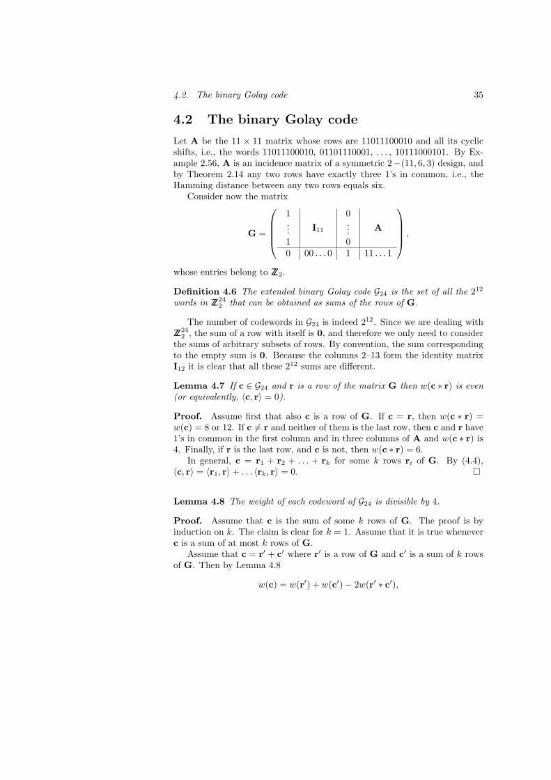
Let A be the 11 × 11 matrix whose rows are 11011100010 and all its cyclicshifts, i.e., the words 11011100010, 01101110001, . . . , 10111000101. By Ex-ample 2.56, A is an incidence matrix of a symmetric 2−(11, 6, 3) design, andby Theorem 2.14 any two rows have exactly three 1’s in common, i.e., theHamming distance between any two rows equals six.

Consider now the matrix

G =

1...1

I11

0...0

A

0 00 . . . 0 1 11 . . . 1

,

whose entries belong to ZZ2.

Definition 4.6 The extended binary Golay code G24 is the set of all the 212

words in ZZ242 that can be obtained as sums of the rows of G.

The number of codewords in G24 is indeed 212. Since we are dealing withZZ24

2 , the sum of a row with itself is 0, and therefore we only need to considerthe sums of arbitrary subsets of rows. By convention, the sum correspondingto the empty sum is 0. Because the columns 2–13 form the identity matrixI12 it is clear that all these 212 sums are different.

Lemma 4.7 If c ∈ G24 and r is a row of the matrix G then w(c ∗ r) is even(or equivalently, 〈c, r〉 = 0).

Proof. Assume first that also c is a row of G. If c = r, then w(c ∗ r) =w(c) = 8 or 12. If c 6= r and neither of them is the last row, then c and r have1’s in common in the first column and in three columns of A and w(c ∗ r) is4. Finally, if r is the last row, and c is not, then w(c ∗ r) = 6.

In general, c = r1 + r2 + . . . + rk for some k rows ri of G. By (4.4),〈c, r〉 = 〈r1, r〉+ . . . 〈rk, r〉 = 0. ¤

Lemma 4.8 The weight of each codeword of G24 is divisible by 4.

Proof. Assume that c is the sum of some k rows of G. The proof is byinduction on k. The claim is clear for k = 1. Assume that it is true wheneverc is a sum of at most k rows of G.

Assume that c = r′ + c′ where r′ is a row of G and c′ is a sum of k rowsof G. Then by Lemma 4.8

w(c) = w(r′) + w(c′)− 2w(r′ ∗ c′),


which is divisible by four, because the first two terms are divisible by 4 bythe induction hypothesis, and the last one by the previous lemma. ¤

If c ∈ G24, we denote by wL(c) the weight of the left half, i.e., the numberof 1’s in the first 12 coordinates, and by wR(c) the weight of the right half.

Theorem 4.9 If c ∈ G24 and c 6= 0, then w(c) ≥ 8. Consequently, if x,y ∈G24 and x 6= y, then d(x,y) ≥ 8.

Proof. We have already shown that the weight of a codeword is divisible byfour. It remains to prove that it cannot be equal to four. Clearly wL(c) iseven for every codeword c: if c is the sum of some i of the first 11 rows thenwL(c) is i for even i and i+1 for odd i. Assume that c ∈ G24 has weight four.

Case 1 wL(c) = 0: Then c is 0 or the last row of G, neither of weightfour.

Case 2 wL(c) = 2: Then c is the sum of one or two rows of G (possiblytogether with the last row), but the sum of two rows of A has always weight6, and hence w(c) ≥ 2 + 6 = 8.

Case 3 wL(c) = 4: Then c is the sum of three or four of the first 11 rows;the last row cannot be involved because wR(c) = 0. If c is a sum of three rowsand r is any other row (of the first 11 rows), then wR(c+ r) = wR(r) = 6 andwL(c + r) = 4 because c + r is a sum of four rows. But then c + r ∈ G24 hasweight 10, contradicting Lemma 4.8. If c is a sum of four rows and r is oneof them, then c = c′ + r where c′ is a sum of three rows. Then wL(c′) = 4and wR(c′) = wR(r) = 6, which again gives a codeword of weight 10.

The last claim immediately follows from (4.3). ¤

Definition 4.10 The binary Golay code G23 is obtained by deleting the firstcoordinate in each codeword of G24.

Theorem 4.11 The code G23 is a perfect 3-error-correcting code.

Proof. Any two codewords in G23 still differ in at least seven coordinates,i.e., G23 is 3-error-correcting. Since 1 + 23 +

(232

)+

(233

)= 211, the Hamming

bound (4.2) holds with equality. ¤

4.3. Steiner systems S(5,8,24) and S(5,6,12) 37

4.3 Steiner systems S(5, 8, 24) and S(5, 6, 12)

Theorem 4.12 There are 759 codewords of weight 8 in G24.

Proof. We show that there are 253 codewords of weight 7 and 506 codewordsof weight 8 in G23, which clearly implies the claim.

Because G23 is perfect, every binary vector of weight 4 is contained inexactly one of the spheres B3(c), c ∈ G23. The sphere B3(0) does not containany of them; and the same is true for B3(c) whenever w(c) ≥ 8. Consequentlyall vectors of weight 4 are contained in the spheres B3(c) where c ∈ G23 andw(c) = 7. Moreover, the distance from of a codeword c of weight 7 to a vectorx of weight 4 is three only if the 1’s in x are in the coordinates where also chas 1’s; hence B3(c) contains exactly

(74

)vectors of weight 4. Therefore the

number of codewords of weight 7 in G23 is(234

)/(74

)= 253.

In the same way consider vectors of weight 5. Exactly 253(75

)of them

are contained in the spheres B3(c) for the codewords c of weight 7, and theremaining ones must be contained in the spheres B3(c) for the codewords ofweight 8, and each such sphere contains

(85

)of them. Therefore the number

of codewords of weight 8 in G23 is ((235

)− 253(75

))/

(85

)= 506. ¤

Theorem 4.13 The words of weight 8 in the code G24 form a Steiner systemS(5, 8, 24).

Proof. Construct a 759 × 24 matrix whose rows are the 759 codewords ofweight 8 and interpret it as the incidence matrix of a design. The number ofblocks is 759, and each block has eight elements of the set T = {1, 2, . . . , 24}.We show that each 5-element subset of B belongs to exactly one of the blocks.

Assume that a 5-element set lies in more than one block. Then thereare two rows in the matrix with at least five 1’s in common. But then theHamming distance between these two rows is at most 6, a contradiction.

On the other hand, each of these 759 blocks contains(85

)5-element subsets,

so altogether the blocks contain 759(85

)=

(245

)5-elements subsets of T , i.e.,

all the 5-element subsets of T . ¤

Theorem 4.14 There is a Steiner system S(5, 6, 12).

Proof. Any given 5-element subset of the set Q = {13, 14, . . . , 24} is con-tained in a unique block of our S(5, 8, 24). By Lemma 4.7 the correspondingrow c in the incidence matrix of S(5, 8, 24) and the last row of G have an evennumber of 1’s in common. They cannot have eight 1’s in common, otherwisetheir sum would give a codeword of weight four in G24. Hence the number of


1’s in common must be six. We can therefore take as blocks of the Steinersystem S(5, 6, 12) all the sets B ∩ Q where B ∈ S(5, 8, 24) and |B ∩ Q| = 6.

¤

From Theorem 3.7 we immediately obtain the following corollary.

Corollary 4.15 There exist Steiner systems S(4, 7, 23) and S(4, 5, 11). ¤

Apart from these four the only currently known Steiner systems S(t, k, v)with k > t ≥ 4 are S(5, 6, 24), S(5, 6, 36), S(5, 7, 28), S(5, 6, 48), S(5, 6, 72),S(5, 6, 84), S(5, 6, 108), S(5, 6, 132), S(5, 6, 168) and S(5, 6, 244), and the 4-designs resulting from Theorem 3.7. It is an open problem whether or notthere exists an infinite number of such Steiner systems.

Bibliography

[1] Anderson, I.: A First Course in Combinatorial Mathematics. Oxford:Oxford University Press, 1989 (2nd edition).

[2] Anderson, I.: Combinatorial Designs: Construction Methods. Chich-ester: Ellis Horwood, 1990. (Together with [1] the primary reference forthese lecture notes.)

[3] Anderson, I.: Combinatorial Designs and Tournaments. Oxford: Ox-ford University Press, 1997.

[4] Beth, T., Jungnickel, D. and Lenz, H.: Design Theory. Cambridge:Cambridge University Press, 1993.

[5] Colbourn, C.J. and Dinitz, J.H.(eds.): The CRC Handbook of Combi-natorial Designs. Boca Raton: CRC Press, 2007 (2nd edition).

[6] Hall, M.: Combinatorial Theory. New York: Wiley, 1986 (2nd edition).

[7] Hardy, G.H. and Wright, E.M.: An Introduction to the Theory of Num-bers. Oxford: Oxford University Press, 1979 (5th edition).

[8] van Lint, J.H.: Introduction to Coding Theory. New York: Springer,1992 (2nd edition).

[9] van Lint, J.H. and Wilson, R.M.: A Course in Combinatorics. Cam-bridge: Cambridge University Press, 1992.

[10] MacWilliams, F.J. and Sloane, N.J.A.: The Theory of Error-CorrectingCodes. Amsterdam: North-Holland, 1977.

[11] Ryser, H.J.: Combinatorial Mathematics. Carus Math. Monograph 14,Math. Assoc. of America, 1963.

39

a short course in combinatorial designs · 1.3 optimal assignment problem ... s3 = fa;dg;s4 =...

Documents