a profile of the free state province: demographics...

Background Paper Series

Background Paper 2005:1(4)

A profile of the Free State province: Demographics,

poverty, inequality and unemployment

Elsenburg August 2005

Overview

The Provincial Decision-Making Enabling (PROVIDE) Project aims to facilitate policy design by supplying policymakers with provincial and national level quantitative policy

information. The project entails the development of a series of databases (in the format of Social Accounting Matrices) for use in Computable General Equilibrium

models.

The National and Provincial Departments of Agriculture are the stakeholders and funders of the PROVIDE Project. The research team is located at Elsenburg in the

Western Cape.

PROVIDE Research Team

Project Leader: Cecilia Punt Senior Researchers: Kalie Pauw Melt van Schoor Young Professional: Bonani Nyhodo Technical Expert: Scott McDonald Associate Researchers: Lindsay Chant Christine Valente

PROVIDE Contact Details

� Private Bag X1 Elsenburg, 7607 South Africa

� [email protected] � +27-21-8085191 � +27-21-8085210

For the original project proposal and a more detailed description of the project,

please visit www.elsenburg.com/provide

PROVIDE Project Background Paper 2005:1(4) August 2005

i © PROVIDE Project

A profile of the Free State province: Demographics, poverty,

inequality and unemployment 1

Abstract

This paper forms part of a series of papers that present profiles of South Africa’s provinces, with a specific focus on key demographic statistics, poverty and inequality estimates, and estimates of unemployment. In this volume comparative statistics are presented for agricultural and non-agricultural households, as well as households from different racial groups, locations (metropolitan, urban and rural areas) and district municipalities of the Free State. Most of the data presented are drawn from the Income and Expenditure Survey of 2000 and the Labour Force Survey of September 2000, while some comparative populations statistics are extracted from the National Census of 2001 (Statistics South Africa). The papers should be regarded as general guidelines to (agricultural) policymakers as to the current socio-economic situation in the Free State, particularly with regard to poverty, inequality and unemployment.

1 The main author of this paper is Kalie Pauw.


ii © PROVIDE Project

Table of Contents

1. Introduction ................................................................................................................ 1 2. Demographics.............................................................................................................. 2

2.1. Spatial distribution of households ........................................................................ 2 2.2. Agricultural households........................................................................................ 4

3. Poverty, inequality and unemployment.................................................................... 6 3.1. Poverty and agriculture......................................................................................... 7 3.2. Inequality in the distribution of income.............................................................. 10 3.3. Employment levels and unemployment.............................................................. 14

4. Conclusions ............................................................................................................... 18 5. References.................................................................................................................. 19

List of Figures Figure 1: District municipalities in the Free State .................................................................... 3 Figure 2: Agricultural household shares by region and race .................................................... 6 Figure 3: Poverty rates by population subgroups ..................................................................... 9 Figure 4: Poverty rates by race and agricultural/non-agricultural population ........................ 10 Figure 5: Lorenz curves for the Free State and South Africa ................................................. 11 Figure 6: Racial representation in the workforce of the Free State ........................................ 16 Figure 7: Unemployment rates by population subgroups ....................................................... 17 Figure 8: Unemployment rates by race and agricultural/non-agricultural population............ 18 List of Tables Table 1: Racial composition of the Free State.......................................................................... 2 Table 2: Population by district municipality and racial group.................................................. 3 Table 3: Population by urban/rural areas and racial group ....................................................... 4 Table 4: Agricultural households by race (broad and strict definitions) .................................. 5 Table 5: Agricultural population by race (broad and strict definitions) ................................... 6 Table 6: Average household incomes in the Free State............................................................ 7 Table 7: Trends in income distribution – 1960 and 1980....................................................... 11 Table 8: Gini decomposition by race and agriculture in the Free State.................................. 13 Table 9: Theil decomposition – agricultural and non-agricultural households ...................... 14


1

1. Introduction

According to the National Census of 2001 the Free State province is home to about 6.0% of South Africa’s population. The Free State has the second lowest total current household income of all the provinces in South Africa. In per capita income terms the province ranks fifth (SSA, 2003a).2 The province is marred by high poverty rates, inequalities in the distribution of income between various population subgroups, and unemployment. Poverty and unemployment in South Africa are often rural phenomena, and given that many of the rural inhabitants are linked to agricultural activities, the various Departments of Agriculture in South Africa have an important role to play in addressing the needs in rural areas. In this paper an overview of the demographics, poverty, inequality and unemployment in the Free State is presented. A strong focus on agriculture and agricultural households is maintained throughout.

There are various sources of demographic data available in South Africa. In addition to the National Census of 2001 (SSA, 2003a), Statistics South Africa conducts a variety of regular surveys. Most suited to this type of study and fairly recent is the Income and Expenditure Survey of 2000 (IES 2000) (SSA, 2002a), which is a source of detailed income and expenditure statistics of households and household members. The twice-yearly Labour Force Survey (LFS) is an important source of employment and labour income data. In this paper we use the LFS September 2000 (LFS 2000:2) (SSA, 2002b) as this survey can be merged with the IES 2000. Although there are some concerns about the reliability of the IES and LFS datasets, whether merged or used separately, as well as the comparability of these with other datasets, one should attempt to work with it as it remains the most recent comprehensive source of household income, employment and expenditure information in South Africa. For a detailed description of the data, as well as data problems and data adjustments made to the version of the dataset used in this paper, refer to PROVIDE (2005a).

This paper is organised as follows. Section 2 presents a brief overview of the spatial distribution of households within the province, while also presenting some estimates of the number of people or households involved in agricultural activities. Section 3 focuses on poverty, inequality and unemployment in the province, while section 4 draws some general conclusions.

2 These population figures and income estimates are based on the Census 2001. Statistics South Africa warns that

the question simply asked about individual income without probing about informal income, income from profits, income in kind etc. As a result they believe this figure may be a misrepresentation of the true income. Comparative figures from the IES 2000 ranks the Free State fifth in terms of total provincial income, and fourth as measured by per capita income.


2

2. Demographics

2.1. Spatial distribution of households

In 2000 the Free State was home to 698,247 households and a total of 2.75 million people (IES/LFS 2000). These estimates are slightly lower than the Census 2001 estimates of 733,302 households (2.71 million people, see Table 1). The discrepancy is partly explained by the population growth experienced between 2000 and 2001, but also points to the outdated IES/LFS 2000 sampling weights.3 Compared to the Census 2001 data African and Coloured people were under-represented, while the other population groups were over-represented in the IES/LFS 2000.

Table 1: Racial composition of the Free State

IES/LFS 2000 Population share Census 2001 Population share African 2,389,480 86.9% 2,381,072 88.0% Coloured 83,351 3.0% 83,192 3.1% Asian/Indian 3,684 0.1% 3,721 0.1% White 273,425 9.9% 238,791 8.8% Total 2,749,939 100.0% 2,706,776 100.0% Sources: IES/LFS 2000 and Census 2001.

The Free State is divided into five district municipalities (see Figure 1), namely Xhariep, Lejweleputswa, Northern Free State, Thabo Mofutsanyane, and Motheo. Bloemfontein, which is located in Motheo, is the provincial capital and is defined as a metropolitan city for the purposes of this paper.4 A subsection of Motheo previously formed part of the former homeland Bophuthatswana, while parts of Thabo Mofutsanyano fell under the QwaQwa homeland. These district municipalities were recently demarcated as directed by the Local Government Municipal Structures Act (1998).5

3 The IES 2000 sampling weights were based on 1996 population estimates. 4 Officially the Demarcation Board declared Pretoria (Tshwane), Johannesburg, East Rand (Ekurhuleni), Durban

(eThekwini), Cape Town and Port Elizabeth (Nelson Mandela) as metropolitan areas. However, in our definition of metropolitan area we include the Vaal (Emfuleni), East London, Pietermaritzburg and Bloemfontein (which includes Botshabelo).

5 See PROVIDE (2005b) for a more detailed discussion of geographical distinctions between households based on former homelands areas, metropolitan areas, and nodal areas for rural development programmes, all of which can be linked to municipal districts.


3

Figure 1: District municipalities in the Free State

Source: Demarcation Board (www.demarcation.org.za).

Table 2 shows the number of people in each district municipality by racial group. Thabo Mofutsanyane is the largest and is home to 27.9% of the population. The Motheo and Lejweleputswa are similar in size, with 25.8% of the population each. This followed by Northyern Free State (16.7%) and Xhariep (3.8%). By far the majority of the population is classified as African (86.9%). The White population makes up 9.9% of the total, while there are very few Coloured (3.0%) and Asian (0.1%) people.

Table 2: Population by district municipality and racial group

African Coloured Asian White Total Percentages Xhariep 76,607 28,386 737 105,730 3.8% Lejweleputswa 627,098 10,100 777 71,054 709,030 25.8% Northern Free State 380,932 18,447 777 58,214 458,370 16.7% Thabo Mofutsanyane 724,031 6,548 1,157 35,017 766,754 27.9% Motheo 580,811 19,869 972 108,404 710,056 25.8% Total 2,389,479 83,350 3,683 273,426 2,749,940 Percentages 86.9% 3.0% 0.1% 9.9% 100.0% Source: IES/LFS 2000

Table 3 shows the number of people in urban and rural areas. Urban areas are divided into metropolitan areas and secondary cities or small towns. One in five people live in metropolitan areas, which includes Bloemfontein and Botshabelo. The majority of the population (72.8%) live in urban areas. This figure is relatively high compared to the national average 63-37 urban-rural split.


4

Table 3: Population by urban/rural areas and racial group

African Coloured Asian White Total Percentages

Metropolitan areas 436,986 19,517 194 91,706 548,403 19.9% Secondary/small towns 1,234,251 56,474 2,332 160,292 1,453,349 52.9% Rural areas 718,243 7,359 1,157 21,427 748,186 27.2% Total 890,272 2,349,596 24,525 723,280 3,987,673 Source: IES/LFS 2000

2.2. Agricultural households

The IES 2000 is one of the only sources of information on home production for home consumption (HPHC) in South Africa, and reports specifically on the productive activities of small, non-commercial subsistence farmers. Respondents were asked to provide estimates of production levels (livestock and produce), as well as the value of goods consumed and sold (see PROVIDE, 2005a for a discussion). This is potentially an important information source to measure the contribution of informal agricultural activities to poor households’ income. On the formal side, employment data, which is available in the IES/LFS 2000, can be used to link households to agriculture. Workers reported both the industry in which they were employed as well as their occupation code.

Statistics South Africa has no formal definition of agricultural households, and hence two definitions are used here, namely a broad definition and a strict definition. Both definitions use a combination of HPHC data and agricultural employment data. Under the broad definition any household that earns income from either formal employment in the agricultural industry or as a skilled agricultural worker, or from sales or consumption of home produce or livestock, is defined as an agricultural household.6 Under the strict definition a household has to earn at least 50% of its household-level income from formal and/or informal agricultural activities. A further way to ‘qualify’ as an agricultural household is when the value of consumption of own produce and livestock is at least 50% of total annual food expenditure.

About 126,077 households (18.1%) in the Free State are involved in HPHC. The national average is 19.3%. This figure includes 114,527 African households, 1,410 Coloured households and 10,141 White households. Slightly fewer households (90,732) earn some share of their income from wages of household members working in agricultural-related industries. The majority of these (84,196) of these households are African, while 1,683 are Coloured and 4,853 are White households. Income differences between these households suggest that the White households are typically the owners or managers of farms, with

6 Note that consumption of own produce or livestock in economic terms can be regarded as an ‘income’ in the

sense that the household ‘buys’ the goods from itself. If it did not produce these goods for own consumption the household would have had to buy it from the market. This treatment of home-consumed production captures the notion of opportunity cost in economics.


5

incomes averaging R505,383. African and Coloured households typically supply farm labour, with average household incomes of R11,545 and R7,507, respectively. When combining households in own production and agricultural employment a total of 181,621 households (26.0%) in the Free State can broadly be defined as agricultural households. Note that some of these households ‘qualify’ as agricultural households on both own production and employment accounts, which is why the figures do not add up. Under the strict definition 96,555 households (13.8%) are defined as agricultural households (see Table 4). The difference is quite large, and is caused in part by the fact that although many households are involved in agricultural activities (mostly own production), it is not a very important income source to many of these households.

Table 4: Agricultural households by race (broad and strict definitions)

Broad definition Strict definition

Agricultural households (column

percentages)

Non-agricultural households (column

percentages)

Agricultural households (column

percentages)

Non-agricultural households (column

percentages) Total (column percentages)

African 167,224 421,850 90,884 498,190 589,074 (92.1%) (81.7%) (94.1%) (82.8%) (84.4%) Coloured 2,501 10,006 1,362 11,145 12,507 (1.4%) (1.9%) (1.4%) (1.9%) (1.8%) Asian 2,596 2,596 2,596 (0.0%) (0.5%) (0.0%) (0.4%) (0.4%) White 11,895 82,175 4,309 89,761 94,070 (6.5%) (15.9%) (4.5%) (14.9%) (13.5%) Total 181,621 516,626 96,555 601,692 698,247 (100.0%) (100.0%) (100.0%) (100.0%) (100.0%) Row percentages 26.0% 74.0% 13.8% 86.2% 100.0%

Source: IES/LFS 2000

The average household size of agricultural households in the Free State ranges from 4.0 (strict) to 4.2 (broad), which is higher than the provincial average of 3.5 members. This means that the provincial share of people living in agricultural households is actually larger than the share of households defined as agricultural. Table 5 shows that between 436,982 and 856,397 people live in agricultural households, representing 15.9% and 31.1% of the provincial population respectively. About 130,853 people in the Free State are classified as agricultural workers, loosely defined here as skilled agriculture workers and/or people working in the agricultural industry, either in an informal or formal capacity, and reporting a positive wage or salary for the year 2000. This figure represents 16.2% of the Free State’s workforce.


6

Table 5: Agricultural population by race (broad and strict definitions)

Population living in agricultural

households (broad) Percentages

Population living in agricultural

households (strict) Percentages

Population defined as

agricultural workers Percentages

African 799,300 (93.3%) 415,209 (95.0%) 120,820 (92.3%) Coloured 21,383 (2.5%) 9,429 (2.2%) 2,931 (2.2%) Asian - (0.0%) - (0.0%) - (0.0%) White 35,714 (4.2%) 12,344 (2.8%) 7,102 (5.4%) Total 856,397 (100.0%) 436,982 (100.0%) 130,853 (100.0%) Source: IES/LFS 2000.

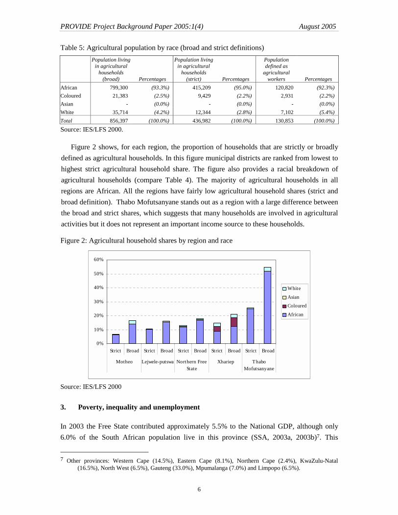
Figure 2 shows, for each region, the proportion of households that are strictly or broadly defined as agricultural households. In this figure municipal districts are ranked from lowest to highest strict agricultural household share. The figure also provides a racial breakdown of agricultural households (compare Table 4). The majority of agricultural households in all regions are African. All the regions have fairly low agricultural household shares (strict and broad definition). Thabo Mofutsanyane stands out as a region with a large difference between the broad and strict shares, which suggests that many households are involved in agricultural activities but it does not represent an important income source to these households.

Figure 2: Agricultural household shares by region and race

0%

10%

20%

30%

40%

50%

60%

Strict Broad Strict Broad Strict Broad Strict Broad Strict Broad

Motheo Lejwele-putswa Northern FreeState

Xhariep ThaboMofutsanyane

White

Asian

Coloured

African


3. Poverty, inequality and unemployment

In 2003 the Free State contributed approximately 5.5% to the National GDP, although only 6.0% of the South African population live in this province (SSA, 2003a, 2003b)7. This

7 Other provinces: Western Cape (14.5%), Eastern Cape (8.1%), Northern Cape (2.4%), KwaZulu-Natal

(16.5%), North West (6.5%), Gauteng (33.0%), Mpumalanga (7.0%) and Limpopo (6.5%).


7

implies that the per capita GDP in the Free State is lower than the national average. According to the IES/LFS 2000 estimate the Free State per capita income was R11,536 in 2000, only slightly lower than the national average of R12,411. Although the Free State is not the poorest province, high levels of poverty and inequality persist as they do in the rest of the country.

Table 6 shows the average household incomes (not per capita) by various subgroups in the Free State. Although some of these averages are based on very few observations, which often lead to large standard errors, the table gives a general idea of how income is distributed between household groups in the province. The average household in the Free State earned R43,281 in 2000 (not shown in the table). White agricultural households earn substantially more than their non-agricultural counterparts, but the same cannot be said for African or Coloured agricultural households. Note that in all the figures and tables that follow agricultural households are defined according to the strict definition. On average agricultural and non-agricultural households report very similar levels of income in the Free State. Coloured agricultural households are worst off, earning on average only R7,820 per annum compared to R11,315 earned by African households. White agricultural households earned substantially more (R737,439). Note that these figures are household-level income figures that are potentially made up of income earned by multiple household members. As such it is not necessarily a reflection of wages of agricultural and non-agricultural workers. Furthermore, the income figure for White agricultural households is based on only 17 sample observations spread between the various municipal districts.

Table 6: Average household incomes in the Free State Agricultural households Non-agricultural households African Coloured Asian White Total African Coloured Asian White Total Xhariep 9,597 9,589 805,900 132,105 15,294 14,434 15,141Lejweleputswa 11,591 241,945 19,935 27,340 9,532 36,000 165,632 45,412Northern Free State 13,747 3,589 2,111,260 140,794 31,132 48,854 56,329 112,473 46,684Thabo M’sanyane 9,217 395,030 21,476 19,693 15,628 80,178 114,043 28,965Motheo 15,739 8,595 27,264 16,283 27,537 70,239 77,087 142,945 52,436

Provincial average 11,315 7,820 737,439 43,671 25,928 39,930 69,623 138,830 43,218

National average 15,014 24,250 132,816 282,151 26,612 29,777 57,284 88,642 166,100 49,990

3.1. Poverty and agriculture

Table 6 shows that Coloured and African agricultural households are considerably worse off than non-agricultural households in terms of income levels. Agricultural households often reside in rural areas and are far removed from more lucrative employment opportunities in urban areas. As a result the National Department of Agriculture places strong emphasis on rural poverty reduction. Various strategies are proposed in the official policy documentation (see Department of Agriculture, 1998). Central to these strategies are (1) an improvement in


8

rural infrastructure, with the aim of giving rural or resource-poor farmers better access to markets, transport, water and electricity, and (2) employment opportunities within agriculture for the poor. The latter can be interpreted either as the creation of employment opportunities within the commercial farming sector by encouraging commercial farmers to increase employment levels or the creation of new business opportunities for small farmers through a process of land restitution.

Various absolute and relative poverty lines are used in South Africa. In recent years the 40th percentile cut-off point of adult equivalent per capita income has become quite a popular poverty line.8 This was equal to R5,057 per annum in 2000 (IES/LFS 2000). This relates to a poverty headcount ratio (defined as the proportion of the population living below the poverty line) for South Africa of 49.8% (IES/LFS 2000).9 The 20th percentile cut-off of adult equivalent income (R2,717 per annum) is sometimes used as the ‘ultra-poverty line’. About 28.2% of the South African population lives below this poverty line.

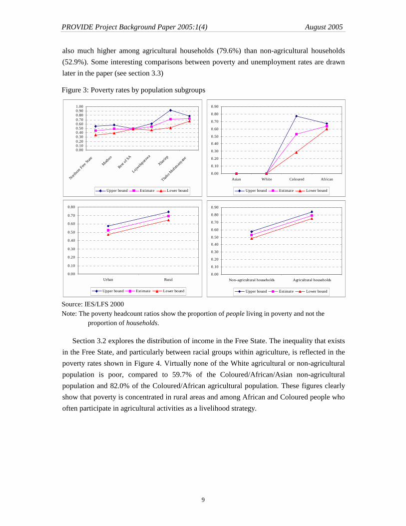
These same national poverty lines are used for the provincial analysis as this allows for comparisons of poverty across provinces. The Free State poverty rate of 57.2% is somewhat higher than the national average, while the ultra-poverty rate is 34.9%. Figure 3 compares poverty rates for various population subgroups (race, municipality, location and agricultural/non-agricultural households). The subgroups are ranked from lowest to highest poverty rates for easy comparison. The upper and lower bands on the graph represent the 95% confidence intervals.

The Northern Free State has the lowest poverty rate (45.4%), followed by Metheo (49.0%). These are the only districts with poverty rates below the national average. Lejweleputswa (53.7%) is slightly above the national average, while Xhariep (71.5%) and Thabo Mofutsanyane (73.0%) are severely impoverished. The relatively wide confidence interval around the poverty estimate for Xhariep is due to the limited number of sample observations for this region.

Poverty rates vary greatly between racial groups. There is virtually no poverty among Asian (very few sample observations) and White people. The poverty estimate shoots up to 53.2% for Coloured people (wide confidence interval due to limited number of sample observations) and 63.9% of Africans. Poverty is also clearly a rural phenomenon, with the rural poverty rate estimated at 69.5% compared to 52.4% in urban areas. The poverty rate is 8 The adult equivalent household size variable, E, is calculated as ( )E A K θα= + , with A the number of adults

per household and K the number of children under the age of 10. In this paper the parameters α and θ are set equal to 0.5 and 0.9 respectively (following May et al., 1995 and others).

9 The poverty headcount ratio is usually calculated using the Foster-Greer-Thorbecke class of decomposable poverty measures (see PROVIDE, 2003 for a discussion). Poverty measures were also calculated to determine the depth and severity of poverty, but we do not report on these in this paper.


9

also much higher among agricultural households (79.6%) than non-agricultural households (52.9%). Some interesting comparisons between poverty and unemployment rates are drawn later in the paper (see section 3.3)

Figure 3: Poverty rates by population subgroups

0.000.100.200.300.400.500.600.700.800.901.00

Northern

Free Stat

e

Motheo

Rest of S

A

Lejwele

putswa

Xhariep

Thabo M

ofutsa

nyane

Upper bound Estimate Lower bound

0.00

0.10

0.20

0.30

0.40

0.50

0.60

0.70

0.80

0.90

Asian White Coloured African


0.00

0.10

0.20

0.30

0.40

0.50

0.60

0.70

0.80

Urban Rural


0.00

0.10

0.20

0.30

0.40

0.50

0.60

0.70

0.80

0.90

Non-agricultural households Agricultural households


Source: IES/LFS 2000 Note: The poverty headcount ratios show the proportion of people living in poverty and not the

proportion of households.

Section 3.2 explores the distribution of income in the Free State. The inequality that exists in the Free State, and particularly between racial groups within agriculture, is reflected in the poverty rates shown in Figure 4. Virtually none of the White agricultural or non-agricultural population is poor, compared to 59.7% of the Coloured/African/Asian non-agricultural population and 82.0% of the Coloured/African agricultural population. These figures clearly show that poverty is concentrated in rural areas and among African and Coloured people who often participate in agricultural activities as a livelihood strategy.


10

Figure 4: Poverty rates by race and agricultural/non-agricultural population

0.00

0.10

0.20

0.30

0.40

0.50

0.60

0.70

0.80

0.90

1.00

White agric White non-agric Afr/Col/Asi non-agric Afr/Col/Asi agric



3.2. Inequality in the distribution of income

This section considers how income is distributed among the population. Various income distribution or inequality measures exist in the literature (see PROVIDE, 2003 for an overview). One approach to measuring inequality is using Lorenz curves. A Lorenz curve plots the cumulative share of households against the cumulative share of income that accrues to those households. In a society where income is perfectly distributed the Lorenz curve is a straight line. When the income distribution is unequal, the Lorenz curve will lie below the ‘line of perfect equality’. Figure 5 shows that the Free State Lorenz curve is always below the South African Lorenz curve, which suggests that income is distributed more unequally in this province than in the rest of the country.


11

Figure 5: Lorenz curves for the Free State and South Africa

0%

10%

20%

30%

40%

50%

60%

70%

80%

90%

100%

0% 10% 20% 30% 40% 50% 60% 70% 80% 90% 100%

Cumulative % of households

Cum

ulat

ive

% o

f inc

ome

Line of perfect equality Lorenz RSA Lorenz FS


The Gini coefficient is perhaps the best known inequality measure and can be derived from the Lorenz curve (see PROVIDE, 2003). Mathematically the Gini coefficient varies between zero and one, although in reality values usually range between 0.20 and 0.30 for countries with a low degree of inequality and between 0.50 and 0.70 for countries with highly unequal income distributions. Table 7 shows the Gini coefficients for various groups of countries. Clearly South Africa’s Gini coefficient, estimated at about 0.69 (IES/LFS 2000), is very high.

Table 7: Trends in income distribution – 1960 and 1980 Group of Countries Gini coefficient: 1960 Gini coefficient: 1980

All non-communist developing countries 0.544 0.602 Low-income countries 0.407 0.450 Middle-income, non-oil-exporting countries 0.603 0.569 Oil-exporting countries 0.575 0.612 Gini coefficient: South Africa (1995)* 0.64 Gini coefficient: South Africa (2000)* 0.70

Source: Adelman (1986) cited in Todaro (1997). Note (*): Author’s calculations based on IES 1995 and IES/LFS 2000. Unfortunately not much can be

read into the apparent increase in inequality since the data sources are not necessarily comparable.

The Free State’s Gini coefficient is 0.72 (IES/LFS 2000), which is slightly higher than the national Gini coefficient. A useful decomposition technique can be used to identify the sources of inequality. From the IES/LFS 2000 a number of household income sources can be identified, namely income from labour (inclab), gross operating surplus (incgos), and transfers from households (inctrans), corporations (inccorp) and government (incgov). Total household


12

income (totinc) is thus defined as totinc = inclab + incgos + inctrans + inccorp + incgov. McDonald et al. (1999) show how the Gini coefficient can be decomposed into elements measuring the inequality in the distribution of these income components. Consider the following equation:

( )( )

( )∑∑

==

=

=

K

kkkk

K

k

k

k

kk

kk

k SGRyFyyFyyFyG

11

)(,cov2)(,cov)(,cov

µµ

µ

The index k represents the income sources. Sk is the share of the kth income source in total income, Gk is the Gini coefficient measuring the inequality in the distribution of income component k and Rk is the Gini correlation of income from source k with total income (see Leibbrandt et al., 2001). The larger the product of these three components, the greater the contribution of income source k to total inequality as measured by G. Sk and Gk are always positive and less than one, while Rk can fall anywhere in the range [-1,1] since it shows how income from source k is correlated with total income.

Table 8 decomposes the Gini coefficient of the Free State. It also gives decompositions for subgroups by race and agricultural households. A clear pattern that emerges for all the subgroups is a very high correlation between the overall Gini and the Gini within income component inclab. Furthermore, inclab typically accounts for about 66% to 78% of total income, except for agricultural households where it only accounts for 42% of income. Consequently, it is not surprising to note that most of the inequality is driven by inequalities in the distribution of labour income. However, this is not the case for agricultural households, where incgos contributes substantially more to overall inequality. Income from gross operating surplus can be interpreted as returns to physical and human capital, and, in an agricultural context, the returns to land owned by the agricultural household.

These results suggest that inequalities within agricultural households are driven primarily by inequalities in the ownership of capital stock and land. This suggests that land reform programmes may be very successful at improving incomes of poor agricultural households. Also significant is the extent to which inequalities in the distribution of wages contribute to inequality among agricultural households. This can be addressed by policies that redistribute wage income to low-income agricultural workers. Also clear from previous tables is that inequality here is driven by inequality between White agricultural farm owners and landless African/Coloured agricultural households that supply labour services.10 10 The difference between inclab and incgos in an agricultural context is problematic. Simkins (2003) notes large

changes in the levels of incgos and inclab between IES 1995 and IES 2000 (incgos fell significantly, while inclab increased), an indication that incgos is possibly underreported due to confusion that may exist among respondents as to whether income earned from self-employment in agriculture should be reported as income from labour or income from GOS.


13

Table 8: Gini decomposition by race and agriculture in the Free State

All households Rk Gk Sk RkGkSk

inclab 0.96 0.77 0.72 0.53 incgos 0.93 0.99 0.10 0.09 inctrans 0.37 0.86 0.04 0.01 inccorp 0.86 0.98 0.07 0.06 incgov 0.35 0.80 0.07 0.02

0.72

African/Coloured/Asian households White households Rk Gk Sk RkGkSk Rk Gk Sk RkGkSk

inclab 0.94 0.75 0.78 0.55 0.86 0.52 0.66 0.30 incgos 0.73 0.98 0.03 0.02 0.89 0.97 0.18 0.15 inctrans 0.36 0.83 0.07 0.02 0.27 0.95 0.02 0.00 inccorp 0.72 0.98 0.02 0.02 0.53 0.91 0.11 0.06 incgov 0.31 0.77 0.10 0.02 0.14 0.89 0.03 0.00

0.64 0.51 Agricultural households Non-agricultural households

Rk Gk Sk RkGkSk Rk Gk Sk RkGkSk inclab 0.96 0.78 0.42 0.31 0.95 0.76 0.77 0.56 incgos 0.99 0.99 0.44 0.44 0.82 0.98 0.04 0.04 inctrans 0.27 0.73 0.03 0.00 0.36 0.87 0.05 0.01 inccorp 0.97 1.00 0.07 0.07 0.83 0.98 0.07 0.05 incgov 0.50 0.76 0.04 0.01 0.31 0.80 0.07 0.02

0.84 0.68 Source: Author’s calculations, IES/LFS 2000

The Gini coefficients suggest that inequality among agricultural households (0.84, with a confidence interval of [0.79, 0.85]) is higher than inequality among non-agricultural households (0.68, with a confidence interval of [0.67, 0.69]). These confidence intervals also do not overlap, which strengthens the belief that inequality is higher among non-agricultural households. An alternative measure of inequality, the Theil index, is very different from other inequality measures, but also confirms this finding. This index is derived from the notion of entropy in information theory (see PROVIDE, 2003). The Theil inequality measure for agricultural households is 2.67 [2.39, 2.77] compared to 0.92 [0.87, 0.97] for non-agricultural households.

These findings raise some interesting questions. Cleary income inequality among agricultural households is a concern. Land restitution has been placed at the top of the government’s agenda to correct inequalities in South African agriculture. Although similar economic empowerment processes are in place in non-agricultural sectors, the process of agricultural land restitution has been highly politicised. The question is will more equality among agricultural households necessarily impact on the overall inequality in the Free State? This question can be answered by decomposing the Theil inequality measure into a measure of inequality within a population subgroup and a measure of inequality between population


14

subgroups. The Theil inequality measure (T) for the Free State population as a whole is 0.81. This figure can be decomposed as follows (see Leibbrandt et al., 2001):

∑ =+= n

i iiB TqTT1

The component TB is the between-group contribution and is calculated in the same way as T but assumes that all incomes within a group are equal. Ti is the Theil inequality measure within the ith group, while qi is the weight attached to each within-group inequality measure. The weight can either be the proportion of income accruing to the ith group or the proportion of the population falling within that group. Table 9 shows the results of a Theil decomposition using income and population weights with agricultural- and non-agricultural households as subgroups.11 The between-group component contributes virtually nothing 0.00 (0.1%) to overall inequality. Although both subgroups have relatively high inequality levels, inequality among agricultural households only contributes 0.37 (32.1%) or 0.43 (35.7%) to overall inequality. Non-agricultural households contribute 0.79 (67.8%) or 0.77 (64.2%) to overall inequality in the Free State, depending on the weights used. These results suggest that a correction of inequalities within agriculture impact on about one third of overall inequality, as most of the inequality in the province is driven by inequalities among non-agricultural households.

Table 9: Theil decomposition – agricultural and non-agricultural households

Income weights qi Ti ∑ =

n

i iiTq1

TB ∑ =+= n

i iiB TqTT1

Agricultural households 0.14 2.67 0.37 Non-agricultural households 0.86 0.92 0.79 Sum 1.16 0.00 1.16

Population weights Agricultural households 0.16 2.67 0.43 Non-agricultural households 0.84 0.92 0.77 Sum 1.20 0.00 1.20 Source: Author’s calculations, IES/LFS 2000 Note: The different decomposition techniques do not necessarily lead to the same overall Theil index.

3.3. Employment levels and unemployment

There are approximately 806,927 workers in the Free State (IES/LFS 2000).12 Statistics South Africa distinguishes between eleven main occupation groups in their surveys. These include

11 The income weight for agricultural households is the total income to agricultural households expressed as a

share of total income of all households in the province. The population weight for agricultural households is expressed as the share of the population living in agricultural households (see Table 2 and Table 5).

12 ‘Workers’ are defined here as those people that report a positive wage for 2000. People who were unemployed at the time of the survey but who have earned some income during the previous year will therefore be captured here as workers. In the unemployment figures reported later the current status of workers is


15

(1) legislators, senior officials and managers; (2) professionals; (3) technical and associate professionals; (4) clerks; (5) service workers and shop and market sales workers; (6) skilled agricultural and fishery workers; (7) craft and related trades workers; (8) plant and machine operators and assemblers; (9) elementary occupations; (10) domestic workers; and (11) not adequately or elsewhere defined, unspecified.

For simplification purposes the occupation groups are aggregated into various skill groups, namely high skilled (1 – 2), skilled (3 – 5), and semi- and unskilled (6 – 10).13 Figure 6 explores the racial composition of the workforce by race and skill and compares these figures with the provincial racial composition. Although the overall racial distribution of the workforce is fairly similar to the racial composition of the province (African workers are slightly under-represented), this is certainly not true for each skill group. African and Coloured workers are typically found in the lower-skilled occupation groups, while White workers are more concentrated around the higher-skilled occupations. Since there are very few Asian workers in the Free State no conclusions can be drawn about their skills distribution. Clearly much still needs to be done in the Free State to bring the racial composition of the workforce more in line with the provincial-level population composition at all skills levels.

reported, irrespective of income earned. Employment figures reported here are therefore higher than the official employment figures.

13 Unspecified workers (code 11) are not included in a specific skill category since the highly dispersed average wage data suggests that these factors may in reality be distributed across the range of skill categories.


16

Figure 6: Racial representation in the workforce of the Free State

Population composition (FS)

African87%

Coloured3%

Asian0%

White10%

Workforce composit ion (FS)

African81%

Coloured3%

Asian0%

White16%

Skills composition by race (FS)

0%

20%

40%

60%

80%

100%

African Coloured Asian White

Semi- & unskilled Skilled High skilled

Racial composition by skills (FS)

0%

20%

40%

60%

80%

100%

Semi- & unskilled Skilled High skilled

African Coloured Asian White


Statistics South Africa uses the following definition of unemployment as its strict (official) definition. The unemployed are those people within the economically active population who: (a) did not work during the seven days prior to the interview, (b) want to work and are available to start work within a week of the interview, and (c) have taken active steps to look for work or to start some form of self-employment in the four weeks prior to the interview. The expanded unemployment rate excludes criterion (c). The Free State has a population of about 2.75 million people of which approximately 798,001 people are employed (see footnote 12). Under the strict (expanded) definition about 1.65 (1.50) million people are not economically active, which implies that 302,819 (456,465) people are unemployed. This translates to an unemployment rate of 27.5% (36.4%), which is slightly higher than the national rate of 26.4% (36.3%) for 2000.14

14 The official (expanded) LFS March and September 2003 (SSA, 2004) unemployment figures are 31.2% and

28.2% for South Africa respectively.


17

In Figure 7 the unemployment rates (official and expanded) are compared for different population subgroups. Unemployment rates are relatively low among White and Asian people, while the difference between the strict and expanded unemployment rates are not that different from each other. However, it rises rapidly for Coloured workers (20.3% - 40.4%). The large difference between the strict and expanded unemployment rates is indicative of a long-term unemployment problem where Coloured people have given up searching for jobs. The African unemployment rate lies between 30.6% and 39.5%. A comparison of the municipal areas shows that all regions have very similar strict unemployment rates. Xhariep shows a fairly large gap between the strict and expanded rates. This municipality is home to the largest contingent of Coloured people in the province, which may explain this result.

Unemployment is also significantly higher in urban areas – an interesting result when compared to South Africa as a whole, where rural unemployment (40.6%) outweighs urban unemployment (33.7%). This may be a result of a steady influx of people, often from other provinces, seeking employment in the Free State’s cities and towns. The Bloemfontein-Botshabelo metropolitan area is located in Motheo, which also has a fairly large unemployment rate. Finally, unemployment is also lower among agricultural households than non-agricultural households.

Figure 7: Unemployment rates by population subgroups

0.0%

5.0%

10.0%

15.0%

20.0%

25.0%

30.0%

35.0%

40.0%

45.0%

White Asian Coloured African

Expanded unemployment rate Strict unemployment rate

0.0%

10.0%

20.0%

30.0%

40.0%

50.0%

60.0%

Thabo M

ofutsa

nyane

Rest of S

A

Lejwele

putswa

Northern

Free Stat

e

Motheo

Xhariep


0.0%

5.0%

10.0%

15.0%

20.0%

25.0%

30.0%

35.0%

40.0%

45.0%

Rural Urban


0.0%

5.0%

10.0%

15.0%

20.0%

25.0%

30.0%

35.0%

40.0%

45.0%

Agricultural households Non-agricultural households




18

A comparison of unemployment rates by race (Asian/Coloured/African and White) and agricultural/non-agricultural households shows that unemployment levels in agriculture are driven mainly by unemployment among Coloured/African workers. Nevertheless, the unemployment rate for Coloured/African agricultural workers is lower than the unemployment rate for Asian/Coloured/African non-agricultural workers. An interesting comparison can be made between Figure 8 and Figure 4. The latter shows that poverty is highest among Coloured/African agricultural households, yet unemployment is lower. One possible explanation for this is inaccurate accounting by agricultural households of the value of goods and services (such as food, clothing and housing) received in kind from employers, which leads to an overestimation of poverty rates. However, this does not take away the fact that agricultural wages are often very low compared to non-agricultural wages. This may explain higher employment levels among agricultural households, but often these people can be classified as the ‘working poor’.

Figure 8: Unemployment rates by race and agricultural/non-agricultural population

0.0%

5.0%

10.0%

15.0%

20.0%

25.0%

30.0%

35.0%

40.0%

45.0%

White agric White non-agric Afr/Col/Asi agric Afr/Col/Asi non-agric



4. Conclusions

The Free State province is relatively small in terms of its population size. The population is largely African (86.9%), lives mainly in urban areas (72.8%) and earns an average per capita income comparable to the national average. Roughly 26.0% of households are involved in agriculture in the broad sense, but only 13.8% are strictly defined as agricultural households. Many of the broadly defined agricultural households are involved in own production, but that these agricultural activities do not represent an important source of household revenue. White agricultural households (mainly farm owners) are very well off and are some of the wealthiest households in the country. African and Coloured agricultural households (mainly landless


19

farm workers), on the other hand, earn very low incomes and are some of the poorest in the country. These factors contribute to the Free State having a very high degree of inequality, especially among agricultural households. The fact that these inequalities can be drawn along racial lines is indicative of discriminatory past and justifies current action taken by government.

Poverty in the Free State is especially pronounced among Coloured and African rural households, many of who are agricultural households. More than 80% of African/Coloured agricultural households are defined as poor. However, at the same time unemployment rates among agricultural households are lower, which suggests that a lot of the poverty can be linked to the phenomenon of the ‘working poor’. Inequalities can be addressed either via redistributing income in the form of higher wages or redistribution of land. Inequalities in the distribution of land and other capital assets has been shown to be one of the important contributors to inequality among agricultural households. However, it has also been suggested that only about one third of overall inequality in the province is ‘explained’ by inequality among agricultural households, and hence a correction of inequalities among agricultural households, although important politically and socially, will have a limited impact on overall inequality in the province.

5. References Department of Agriculture (1998). Agricultural Policy in South Africa. A Discussion

Document, Pretoria. Leibbrandt, M., Woolard, I. and Bhorat, H. (2001). "Understanding contemporary household

inequality in South Africa." In Fighting Poverty. Labour Markets and Inequality in South Africa, edited by Bhorat, H., Leibbrandt, M., Maziya, M., Van der Berg, S. and Woolard, I. Cape Town: UCT Press.

May, J., Carter, M.R. and Posel, D. (1995). "The composition and persistence of poverty in rural South Africa: an entitlements approach," Land and Agricultural Policy Centre Policy Paper No. 15.

McDonald, S., Piesse, J. and Van Zyl, J. (1999). "Exploring Income Distribution and Poverty in South Africa," South African Journal of Economics, 68(3): 423-454.

PROVIDE (2003). "Measures of Poverty and Inequality. A Reference Paper," PROVIDE Technical Paper Series, 2003:4. PROVIDE Project, Elsenburg. Available online at www.elsenburg.com/provide.

PROVIDE (2005a). "Creating an IES-LFS 2000 Database in Stata," PROVIDE Technical Paper Series, 2005:1. PROVIDE Project, Elsenburg. Available online at www.elsenburg.com/provide.

PROVIDE (2005b). "Forming Representative Household Groups in a SAM," PROVIDE Technical Paper Series, 2005:2. PROVIDE Project, Elsenburg. Available online at www.elsenburg.com/provide.

Simkins, C. (2003). "A Critical Assessment of the 1995 and 2000 Income and Expenditure Surveys as Sources of Information on Incomes," Mimeo.

SSA (2002a). Income and Expenditure Survey 2000, Pretoria: Statistics South Africa. SSA (2002b). Labour Force Survey September 2000, Pretoria: Statistics South Africa.


20

SSA (2003a). Census 2001, Pretoria: Statistics South Africa. SSA (2003b). Gross Domestic Product, Statistical Release P0441, 25 November 2003,

Pretoria: Statistics South Africa. SSA (2004). Labour Force Survey, September 2003, Pretoria: Statistics South Africa. Todaro, M.P. (1997). Economic Development, 6th Edition. Longman: London.

Background Papers in this Series Number Title Date BP2003: 1 Multivariate Statistical Techniques September 2003 BP2003: 2 Household Expenditure Patterns in South Africa –

1995 September 2003

BP2003: 3 Demographics of South African Households – 1995 September 2003 BP2003: 4 Social Accounting Matrices September 2003 BP2003: 5 Functional forms used in CGE models: Modelling

production and commodity flows September 2003

BP2005: 1, Vol. 1 – 10

Provincial Profiles: Demographics, poverty, inequality and unemployment (Nine Provinces and National)

June 2005

Other PROVIDE Publications Technical Paper Series Working Paper Series Research Reports

a profile of the free state province: demographics...

Documents