a new min-max regret robust optimization approach for ...nau/adversarial/program/posters/...kk k...

A New Min-Max Regret Robust Optimization Approach for Solving Two-Stages Mixed Integer Linear Optimization

Problems with Full Factorial Scenario Design

Tiravat Assavapokee(1), Matthew Realff(2) and Jane Ammons(3)

(1) Industrial Engineering (2) Chemical & Biomolecular EngineeringUniversity of Houston Georgia Institute of Technology Houston, Texas 77204 Atlanta, Georgia 30332-0100

(3) Industrial & Systems EngineeringGeorgia Institute of TechnologyAtlanta, Georgia 30332-0205

Workshop on Decision Making in Adversarial DomainsMay 23rd, 2005

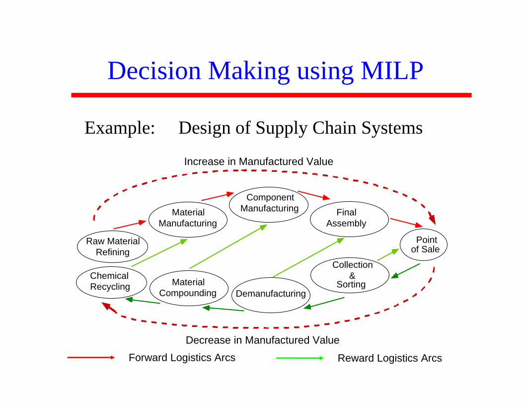
Decision Making using MILP

Refining

MaterialManufacturing

ComponentManufacturing Final

Assembly

of Sale

Increase in Manufactured Value

Collection&

SortingDemanufacturing

Decrease in Manufactured Value

ChemicalRecycling Material

Compounding

Forward Logistics Arcs

Point

Reward Logistics Arcs

Raw Material

Example: Design of Supply Chain Systems

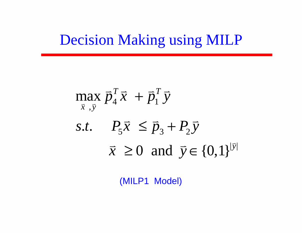
Decision Making using MILP

(MILP1 Model)

4 1,

5 3 2| |

max

. .

0 and 0,1

T T

x y

y

p x p y

s t P x p P y

x y

+

≤ +

≥ ∈

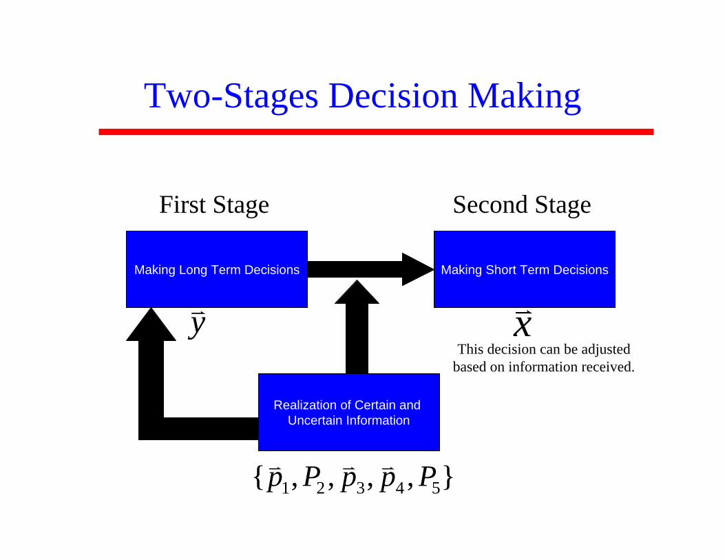
Two-Stages Decision Making

y xMaking Long Term Decisions Making Short Term Decisions

First Stage Second Stage

Realization of Certain and Uncertain Information

1 2 3 4 5 , , , , p P p p P

This decision can be adjusted based on information received.

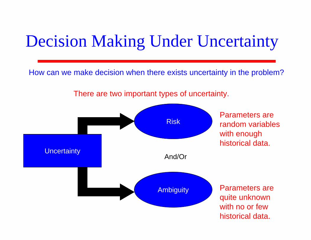
Decision Making Under Uncertainty

How can we make decision when there exists uncertainty in the problem?

Uncertainty

Risk

Ambiguity

And/Or

There are two important types of uncertainty.

Parameters are random variables with enough historical data.

Parameters are quite unknown with no or few historical data.

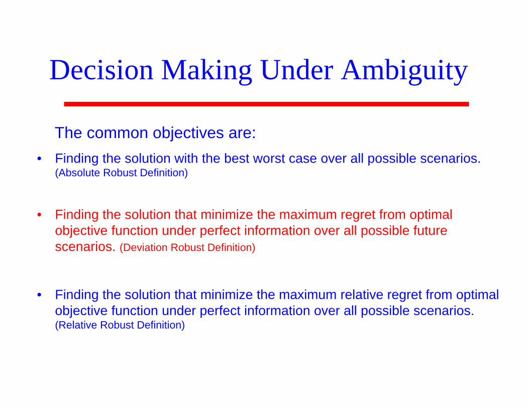
Decision Making Under Ambiguity

The common objectives are:• Finding the solution with the best worst case over all possible scenarios.

(Absolute Robust Definition)

• Finding the solution that minimize the maximum regret from optimal objective function under perfect information over all possible future scenarios. (Deviation Robust Definition)

• Finding the solution that minimize the maximum relative regret from optimal objective function under perfect information over all possible scenarios.(Relative Robust Definition)

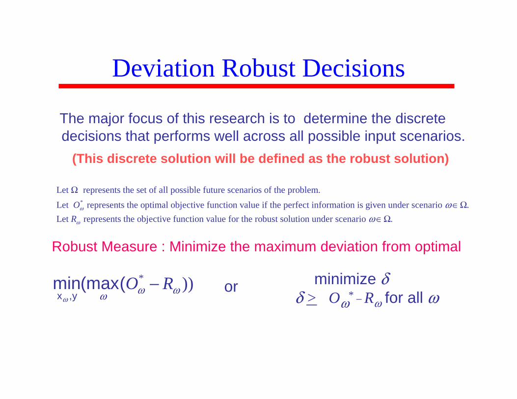
Deviation Robust Decisions

The major focus of this research is to determine the discrete decisions that performs well across all possible input scenarios.

(This discrete solution will be defined as the robust solution)

*

Let represents the set of all possible future scenarios of the problem.Let represents the optimal objective function value if the perfect information is given under scenario .Let represe

OR

ω

ω

ωΩ

∈Ωnts the objective function value for the robust solution under scenario .ω ∈Ω

Robust Measure : Minimize the maximum deviation from optimal

minimize δδ > Oω

* _ Rω for all ω))*

ωωωω

RO −(max(miny,x

or

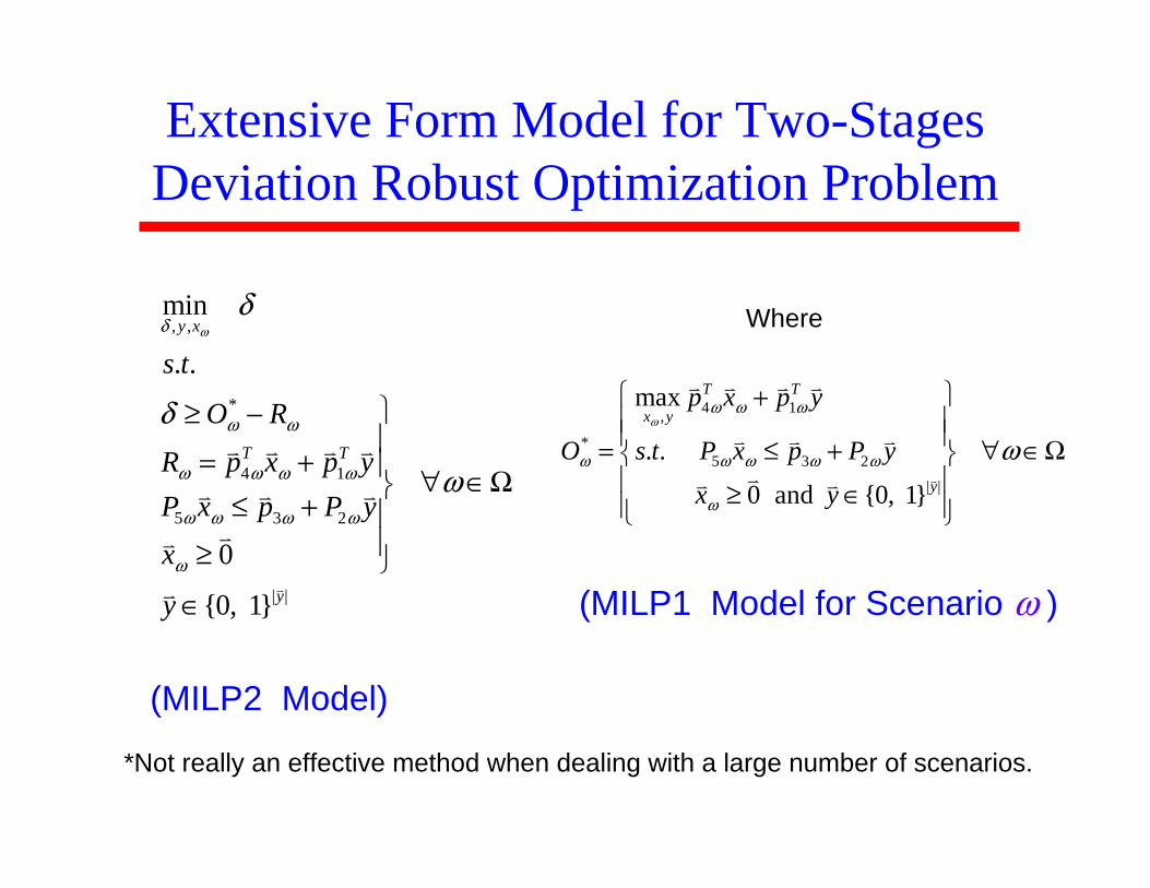
Extensive Form Model for Two-Stages Deviation Robust Optimization Problem

, ,

*

4 1

5 3 2

| |

min

. .

0

0, 1

y x

T T

y

s t

O R

R p x p yP x p P yx

y

ωδ

ω ω

ω ω ω ω

ω ω ω ω

ω

δ

δ

ω

⎫≥ −⎪

= + ⎪ ∀ ∈Ω⎬≤ + ⎪

⎪≥ ⎭∈

4 1,

*5 3 2

| |

max

. .

0 and 0, 1

T T

x y

y

p x p y

O s t P x p P y

x y

ωω ω ω

ω ω ω ω ω

ω

ω

⎧ ⎫+⎪ ⎪⎪ ⎪= ≤ + ∀ ∈Ω⎨ ⎬⎪ ⎪≥ ∈⎪ ⎪⎩ ⎭

Where

(MILP2 Model)

(MILP1 Model for Scenario ω )

*Not really an effective method when dealing with a large number of scenarios.

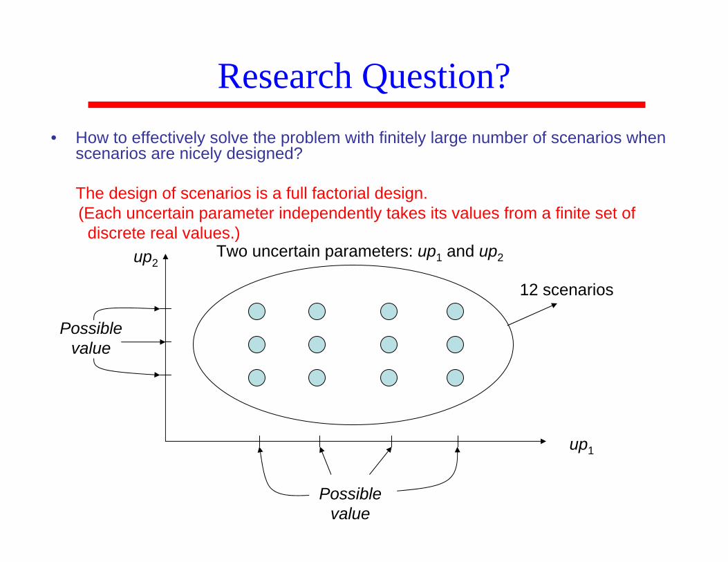
• How to effectively solve the problem with finitely large number of scenarios when scenarios are nicely designed?

The design of scenarios is a full factorial design. (Each uncertain parameter independently takes its values from a finite set of

discrete real values.)

Research Question?

up1

up2

Possible value

Two uncertain parameters: up1 and up2

Possible value

12 scenarios

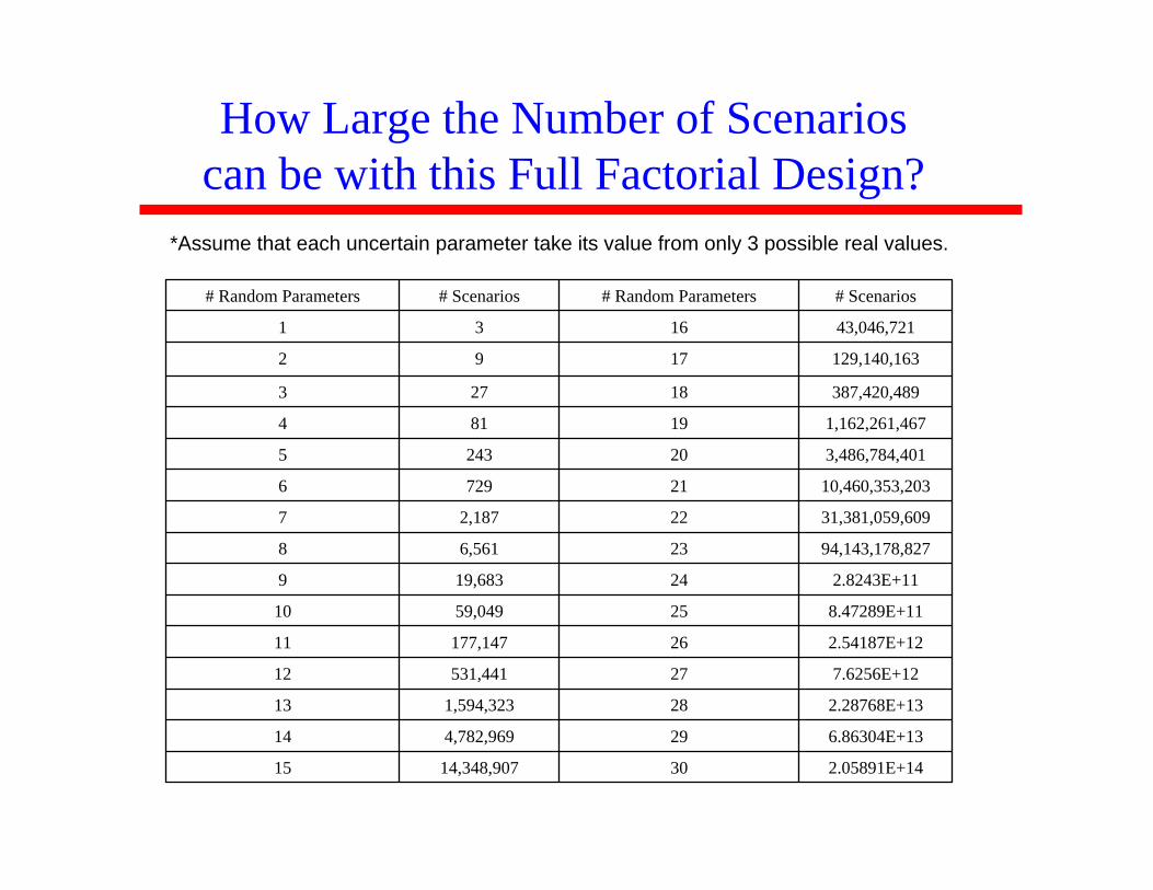
How Large the Number of Scenarioscan be with this Full Factorial Design?

*Assume that each uncertain parameter take its value from only 3 possible real values.

2.05891E+143014,348,90715

6.86304E+13294,782,96914

2.28768E+13281,594,32313

7.6256E+1227531,44112

2.54187E+1226177,14711

8.47289E+112559,04910

2.8243E+112419,6839

94,143,178,827236,5618

31,381,059,609222,1877

10,460,353,203217296

3,486,784,401202435

1,162,261,46719814

387,420,48918273

129,140,1631792

43,046,7211631

# Scenarios# Random Parameters# Scenarios# Random Parameters

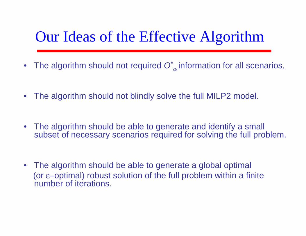
Our Ideas of the Effective Algorithm

• The algorithm should not required O*ω information for all scenarios.

• The algorithm should not blindly solve the full MILP2 model.

• The algorithm should be able to generate and identify a small subset of necessary scenarios required for solving the full problem.

• The algorithm should be able to generate a global optimal (or ε−optimal) robust solution of the full problem within a finite number of iterations.

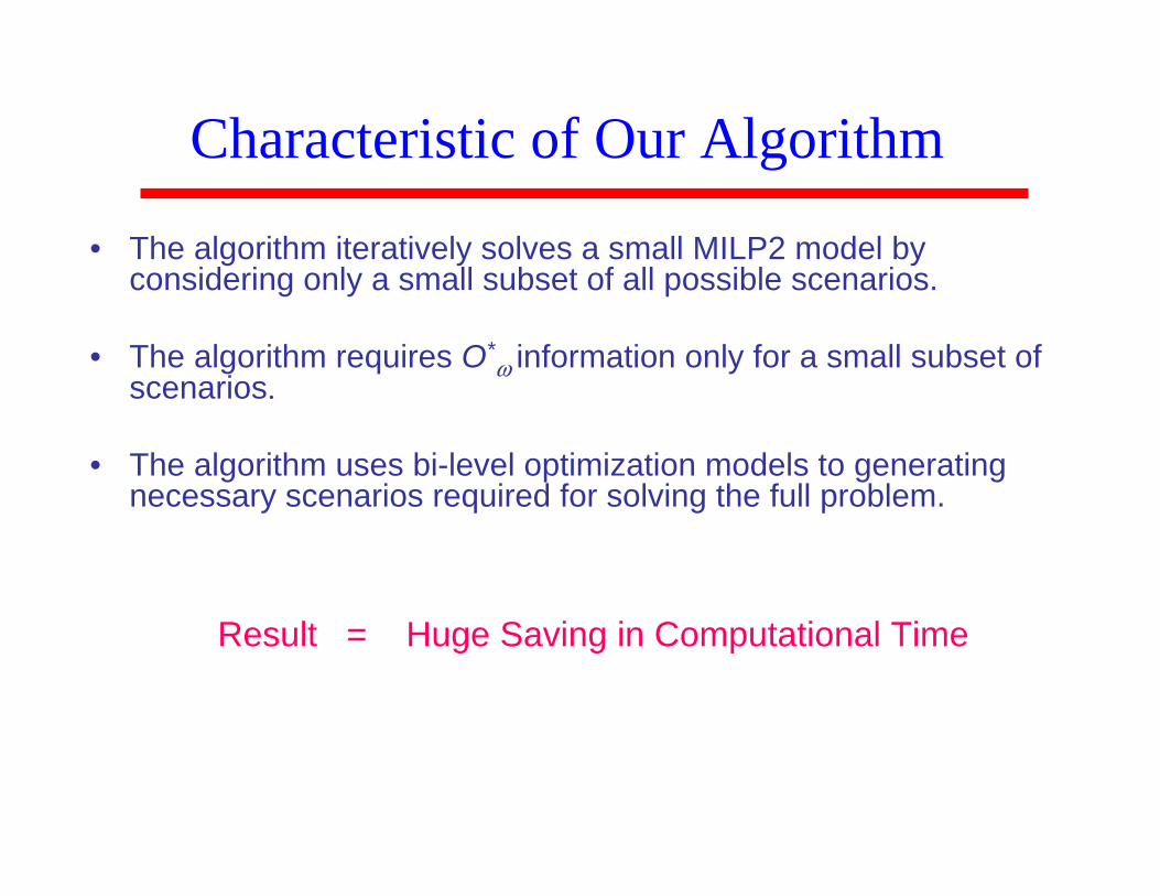
Characteristic of Our Algorithm

• The algorithm iteratively solves a small MILP2 model by considering only a small subset of all possible scenarios.

• The algorithm requires O*ω information only for a small subset of

scenarios.

• The algorithm uses bi-level optimization models to generating necessary scenarios required for solving the full problem.

Result = Huge Saving in Computational Time

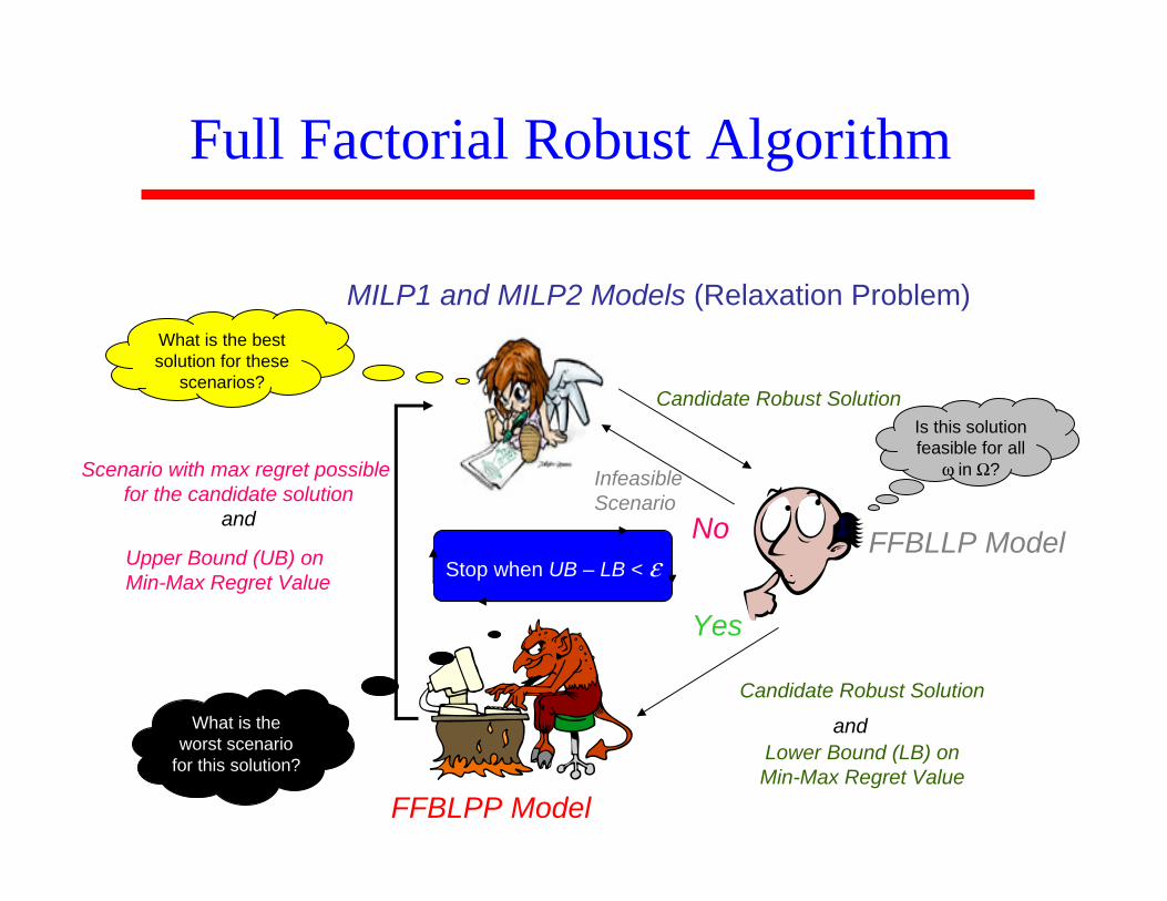
Full Factorial Robust Algorithm

MILP1 and MILP2 Models (Relaxation Problem)

FFBLPP Model

Scenario with max regret possible for the candidate solution

and

Upper Bound (UB) on Min-Max Regret Value

Is this solution feasible for all

ω in Ω?

Candidate Robust Solution

Lower Bound (LB) on Min-Max Regret Value

and

Candidate Robust Solution

Infeasible Scenario

FFBLLP ModelNo

Yes

What is the worst scenario

for this solution?

What is the best solution for these

scenarios?

Stop when UB – LB < ε

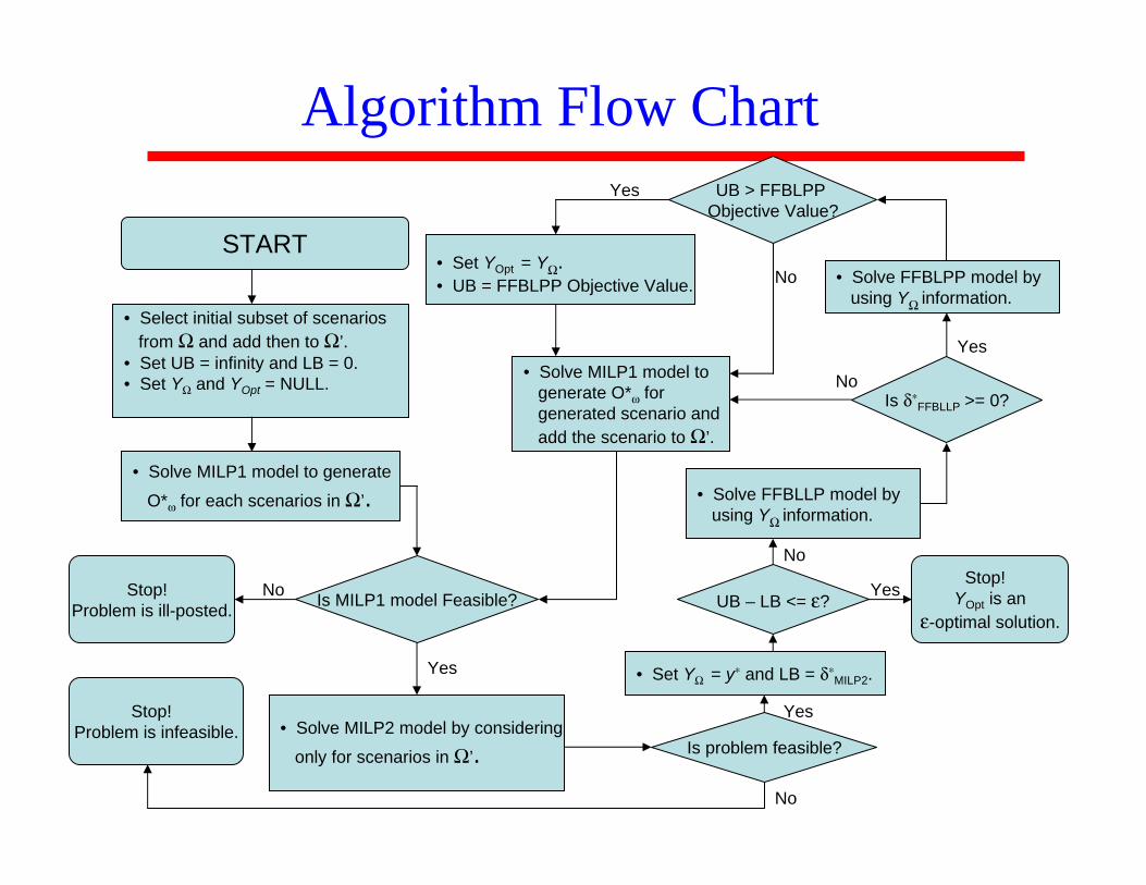
Algorithm Flow Chart

• Select initial subset of scenarios from Ω and add then to Ω’.

• Set UB = infinity and LB = 0.• Set YΩ and YOpt = NULL.

• Solve MILP1 model to generate

O*ω for each scenarios in Ω’.

• Solve MILP2 model by considering

only for scenarios in Ω’.

Is MILP1 model Feasible?

START

Stop! Problem is ill-posted.

• Set YΩ = y∗ and LB = δ∗MILP2.

Is problem feasible?

Stop! Problem is infeasible.

• Solve FFBLLP model by using YΩ information.

Is δ∗FFBLLP >= 0?

No

Yes

No

Yes

• Solve MILP1 model to generate O*ω for generated scenario and add the scenario to Ω’.

No

Yes

• Solve FFBLPP model by using YΩ information.

UB – LB <= ε?

No

YesStop!

YOpt is anε-optimal solution.

UB > FFBLPP Objective Value?

• Set YOpt = YΩ.• UB = FFBLPP Objective Value. No

Yes

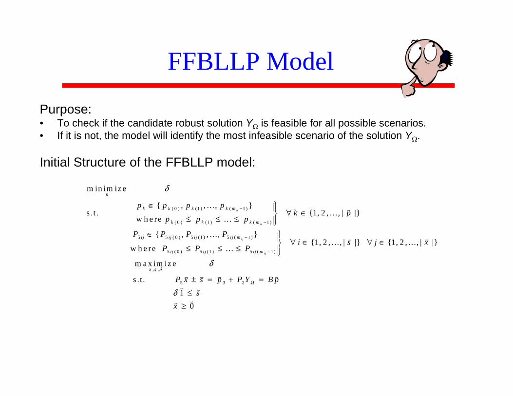
FFBLLP Model

Purpose:• To check if the candidate robust solution YΩ is feasible for all possible scenarios.• If it is not, the model will identify the most infeasible scenario of the solution YΩ.

Initial Structure of the FFBLLP model:

( 0 ) (1 ) ( 1 )

( 0 ) (1 ) ( 1 )

5 5 ( 0 ) 5 (1 ) 5 ( 1 )

m in im iz e

, , . . . , s .t . 1, 2 , . . . , | |

w h e re .. .

, , . . . ,

k

k

ij

p

k k k k m

k k k m

ij ij ij ij m

p p p pk p

p p p

P P P P

δ

−

−

−

∈ ⎫⎪ ∀ ∈⎬≤ ≤ ≤ ⎪⎭∈

5 ( 0 ) 5 (1 ) 5 ( 1 )

, ,

5 3 2

1, 2 , .. . , | | 1, 2 , .. . , | | w h e re .. .

m a x im iz e

s .t .

i ji j ij ij m

x s

i s j xP P P

P x s p P Y B pδ

δ−

Ω

⎫⎪ ∀ ∈ ∀ ∈⎬≤ ≤ ≤ ⎪⎭

± = + =

1 0

sxδ ≤

≥

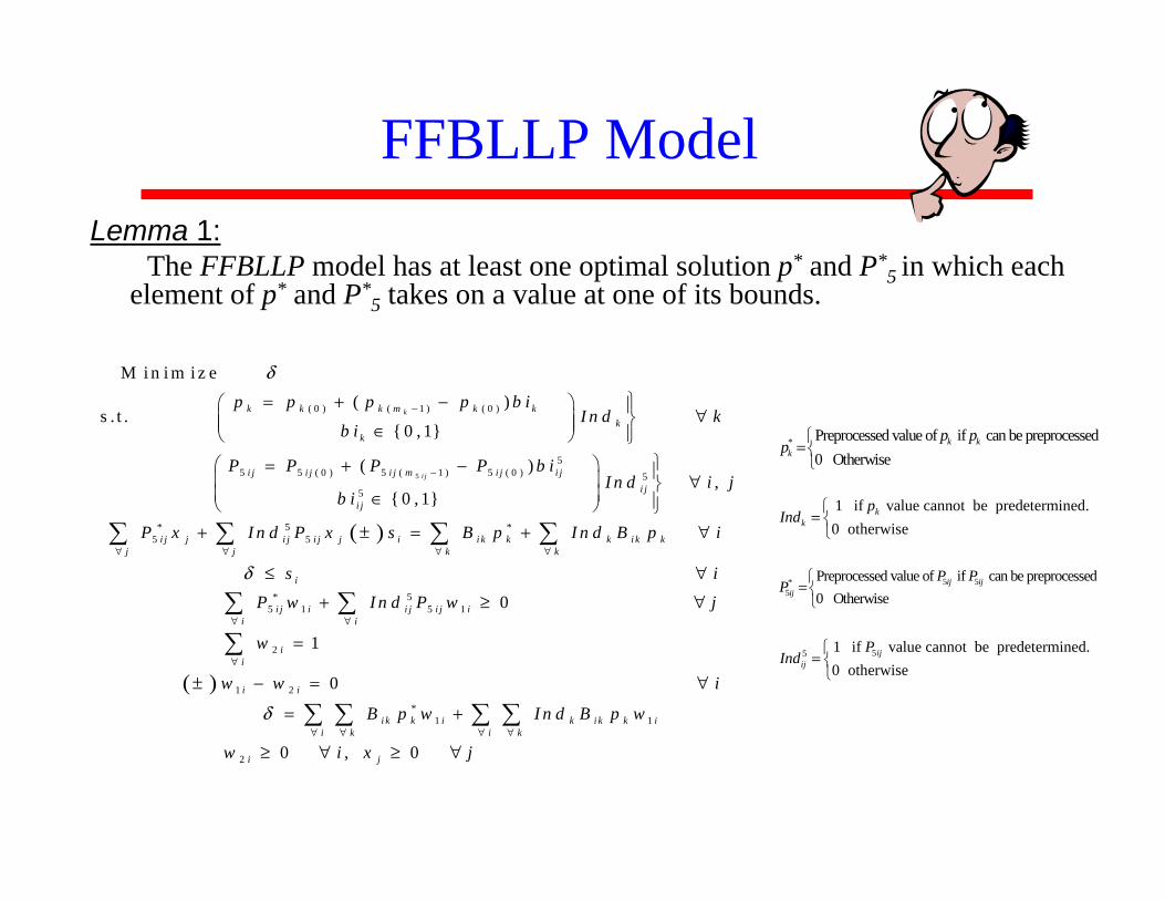
FFBLLP ModelLemma 1:

The FFBLLP model has at least one optimal solution p* and P*5 in which each

element of p* and P*5 takes on a value at one of its bounds.

5

( 0 ) ( 1 ) ( 0 )

55 5 ( 0 ) 5 ( 1 ) 5 ( 0 )

M i n i m i z e

( ) s . t .

0 , 1

( )

k

i j

k k k m k kk

k

i j i j i j m i j i j

i

p p p p b iI n d k

b i

P P P P b i

b i

δ

−

−

⎫= + −⎛ ⎞ ⎪ ∀⎜ ⎟ ⎬⎜ ⎟∈ ⎪⎝ ⎠ ⎭

= + −

( )

55

* 5 *5 5

, 0 , 1

i jj

i j j i j i j j i i k k k i k kj j k k

i

I n d i j

P x I n d P x s B p I n d B p i

s iδ∀ ∀ ∀ ∀

⎫⎛ ⎞ ⎪⎜ ⎟ ∀⎬⎜ ⎟∈ ⎪⎝ ⎠ ⎭+ ± = + ∀

≤ ∀

∑ ∑ ∑ ∑

( )

* 55 1 5 1

2

1 2

*

0

1

0

i j i i j i j ii i

ii

i i

i k k

P w I n d P w j

w

w w i

B pδ

∀ ∀

∀

+ ≥ ∀

=

± − = ∀

=

∑ ∑

∑

1 1

2 0 , 0

i k i k k ii k i k

i j

w I n d B p w

w i x j∀ ∀ ∀ ∀

+

≥ ∀ ≥ ∀

∑ ∑ ∑ ∑

1 if value cannot be predetermined.0 otherwise

kk

pInd

⎧= ⎨⎩

55 1 if value cannot be predetermined.0 otherwise

ijij

PInd

⎧= ⎨⎩

* Preprocessed value of if can be preprocessed0 Otherwise

k kk

p pp

⎧=⎨⎩

5 5*5

Preprocessed value of if can be preprocessed0 Otherwise

ij ijij

P PP

⎧= ⎨⎩

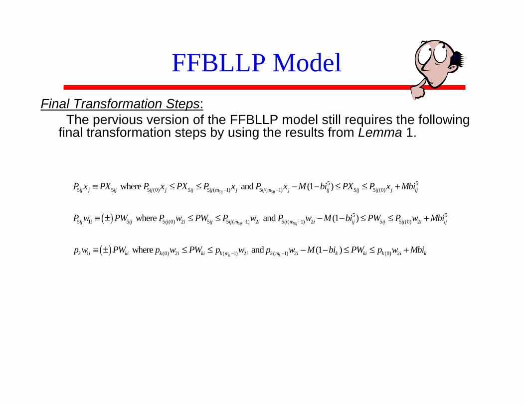
FFBLLP ModelFinal Transformation Steps:

The pervious version of the FFBLLP model still requires the following final transformation steps by using the results from Lemma 1.

( )

5 5

5 5

5 55 5 5 (0) 5 5 ( 1) 5 ( 1) 5 5 (0)

55 1 5 5 (0) 2 5 5 ( 1) 2 5 ( 1) 2 5 5 (0)

where and (1 )

where and (1 )

ij ij

ij ij

ij j ij ij j ij ij m j ij m j ij ij ij j ij

ij i ij ij i ij ij m i ij m i ij ij ij

P x PX P x PX P x P x M bi PX P x Mbi

P w PW P w PW P w P w M bi PW P

− −

− −

≡ ≤ ≤ − − ≤ ≤ +

≡ ± ≤ ≤ − − ≤ ≤

( )

52

1 (0) 2 ( 1) 2 ( 1) 2 (0) 2 where and (1 )k k

i ij

k i ki k i ki k m i k m i k ki k i k

w Mbi

p w PW p w PW p w p w M bi PW p w Mbi− −

+

≡ ± ≤ ≤ − − ≤ ≤ +

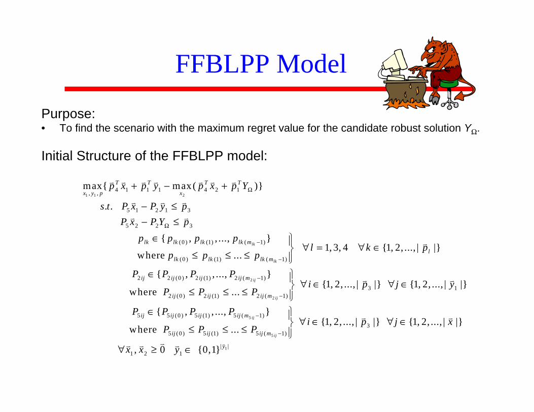
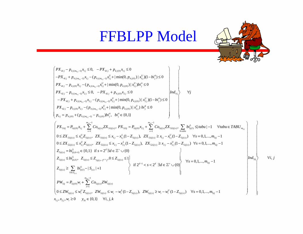
FFBLPP Model

Purpose:• To find the scenario with the maximum regret value for the candidate robust solution YΩ.

Initial Structure of the FFBLPP model:

1 1 24 1 1 1 4 2 1, ,

5 1 2 1 3

5 2 2 3

(0 ) (1) ( 1)

(0 ) (1) ( 1)

max max( )

. .

, , ...,

where ...lk

lk

T T T T

x y p x

lk lk lk lk m

lk lk lk m

p x p y p x p Y

s t P x P y pP x P Y p

p p p p

p p p

Ω

Ω

−

−

+ − +

− ≤− ≤

∈ ⎫⎪⎬≤ ≤ ≤ ⎪⎭

2

2

2 2 (0 ) 2 (1) 2 ( 1)

3 12 (0 ) 2 (1) 2 ( 1)

1, 3, 4 1, 2, ..., | |

, , ..., 1, 2, ..., | | 1, 2, ..., | |

where ...

ij

ij

l

ij ij ij ij m

ij ij ij m

l k p

P P P Pi p j y

P P P−

−

∀ = ∀ ∈

∈ ⎫⎪ ∀ ∈ ∀ ∈⎬≤ ≤ ≤ ⎪⎭

5

5

1

5 5 (0 ) 5 (1) 5 ( 1)

35 (0 ) 5 (1) 5 ( 1)

| |1 2 1

, , ..., 1, 2, ..., | | 1, 2, ..., | |

where ...

, 0 0,1

ij

ij

ij ij ij ij m

ij ij ij m

y

P P P Pi p j x

P P P

x x y

−

−

∈ ⎫⎪ ∀ ∈ ∀ ∈⎬≤ ≤ ≤ ⎪⎭∀ ≥ ∈

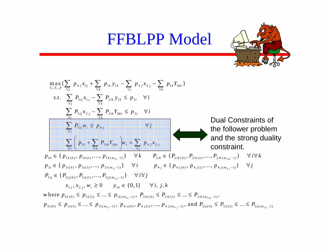
FFBLPP Model

1 14 1 1 1 4 2 1, ,

5 1 2 1 3

5 2 2 3

5 4

m ax

. .

j j k k j j k kx y p j k j k

ij j ik k ij k

ij j ik k ij k

ij i ji

p x p y p x p Y

s t P x P y p i

P x P Y p i

P w p j

Ω∀ ∀ ∀ ∀

∀ ∀

Ω∀ ∀

∀

+ − −

− ≤ ∀

− ≤ ∀

≥ ∀

∑ ∑ ∑ ∑

∑ ∑

∑ ∑

∑

1 2

3

3 2 4 2

1 1 ( 0 ) 1 (1) 1 ( 1) 2 2 ( 0 ) 2 (1) 2 ( 1)

3 3 ( 0 ) 3 (1) 3 ( 1) 4 4 ( 0 ) 4

, , ..., , , ...,

, , ..., ,k ik

i

i ik k i j ji k j

k k k k m ik ik ik ik m

i i i i m j j

p P Y w p x

p p p p k P P P P i k

p p p p i p p p

Ω∀ ∀ ∀

− −

−

⎛ ⎞+ =⎜ ⎟⎝ ⎠

∈ ∀ ∈ ∀ ∀

∈ ∀ ∈

∑ ∑ ∑

4

5

1 2

(1) 4 ( 1)

5 5 ( 0 ) 5 (1) 5 ( 1)

1 2 1

1 ( 0 ) 1 (1) 1 ( 1) 2 ( 0 ) 2 (1) 2 ( 1)

3 ( 0 )

, ...,

, , ...,

, , 0 0,1 , ,

w here ... , ... ,

j

ij

k ik

j j m

ij ij ij ij m

j j i k

k k k m ik ik ik m

i

p j

P P P P i j

x x w y i j k

p p p P P P

p

−

−

− −

∀

∈ ∀ ∀

≥ ∈ ∀

≤ ≤ ≤ ≤ ≤ ≤

3 4 53 (1) 3 ( 1) 4 ( 0 ) 4 (1) 4 ( 1) 5 ( 0 ) 5 (1) 5 ( 1)... , , , ..., , and ...i j iji i m j j j m ij ij ij mp p p p p P P P− − −≤ ≤ ≤ ≤ ≤ ≤

Dual Constraints of the follower problem and the strong duality constraint.

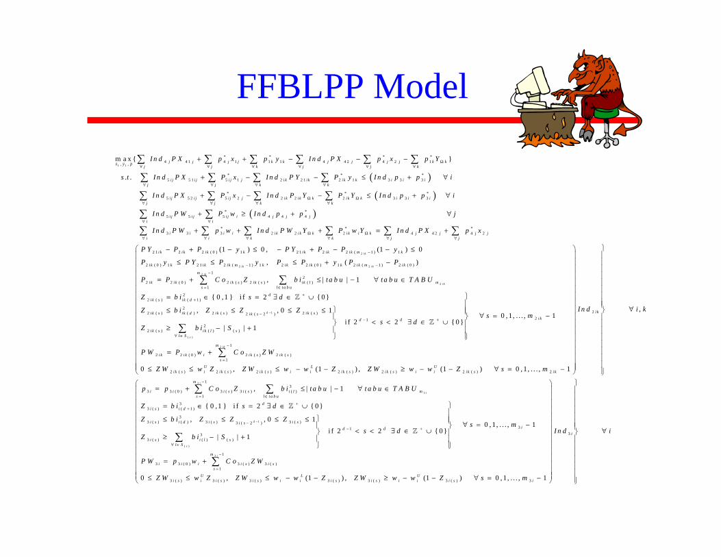
FFBLPP Model

( )1 1

* * * *4 4 1 4 1 1 1 4 4 2 4 2 1, ,

* * *5 5 1 5 1 2 2 1 2 1 3 3 3

5 5 2

m a x

. .

j j j j k k j j j j k kx y p j j k j j k

i j i j i j j i k i k i k k i i ij j k k

i j

I n d P X p x p y I n d P X p x p Y

s t I n d P X P x I n d P Y P y I n d p p i

I n d P X

Ω∀ ∀ ∀ ∀ ∀ ∀

∀ ∀ ∀ ∀

+ + − − −

+ − − ≤ + ∀

∑ ∑ ∑ ∑ ∑ ∑

∑ ∑ ∑ ∑

( )( )

* * *5 2 2 2 2 3 3 3

* *5 5 5 4 4 4

*3 3 3

i j i j j i k i k k i k k i i ij j k k

i j i j i j i j j ji i

i i ii

P x I n d P Y P Y I n d p p i

I n d P W P w I n d p p j

I n d P W p w

Ω Ω∀ ∀ ∀ ∀

∀ ∀

∀

+ − − ≤ + ∀

+ ≥ + ∀

+

∑ ∑ ∑ ∑

∑ ∑

∑

2

2 2

* *2 2 2 4 4 2 4 2

2 1 2 2 ( 0 ) 1 2 1 2 2 ( 1 ) 1

2 ( 0 ) 1 2 1 2 ( 1 ) 1 2 2 ( 0 ) 1 2 (

(1 ) 0 , (1 ) 0

, (

i k

i k i k

i i k i k k i k i k j j j ji k k j j

i k i k i k k i k i k i k m k

i k k i k i k m k i k i k k i k m

I n d P W Y P w Y I n d P X p x

P Y P P y P Y P P y

P y P Y P y P P y P

Ω Ω∀ ∀ ∀ ∀ ∀

−

−

+ + = +

− + − ≤ − + − − ≤

≤ ≤ ≤ +

∑ ∑ ∑ ∑ ∑

2

2

1

1 ) 2 ( 0 )

12

2 2 ( 0 ) 2 ( ) 2 ( ) ( )1

22 ( ) ( 1 )

22 ( ) ( ) 2 ( ) 2 ( )2 ( 2 )

2 ( )

)

, | | 1

0 ,1 i f 2 0

, , 0 1

i k

i k

d

i k

m

i k i k i k s i k s i k l ms l t a b u

dik s i k d

ik s i k d i k s i k si k s

i k s i

P

P P C o Z b i t a b u t a b u T A B U

Z b i s d

Z b i Z Z Z

Z b i

−

−

−

= ∈

++

−

−

= + ≤ − ∀ ∈

= ∈ = ∃ ∈ ∪

≤ ≤ ≤ ≤

≥

∑ ∑

( )

2

212

( ) ( )

1

2 2 ( 0 ) 2 ( ) 2 ( )1

2 ( ) 2 ( ) 2 ( ) 2 ( ) 2 ( ) 2 ( )

0 , 1, . . . , 1 i f 2 2 0

| | 1

0 , (1 ) , (1

s

i k

i kd d

k l sl S

m

i k i k i i k s i k ss

U L Ui k s i i k s i k s i i i k s i k s i i i k s

s ms d

S

P W P w C o Z W

Z W w Z Z W w w Z Z W w w Z

− +

∀ ∈

−

=

⎫⎪

⎫ ⎪⎪ ∀ = −⎪ ⎬< < ∃ ∈ ∪⎬ ⎪− + ⎪ ⎪

⎪⎭ ⎭

= +

≤ ≤ ≤ − − ≥ − −

∑

∑

3

3

2

2

13

3 3 ( 0 ) 3 ( ) 3 ( ) ( )1

3 ( ) (

,

) 0 , 1, . . . , 1

, | | 1

i

i

i k

i k

m

i i i s i s i l ms l t a b u

i s i

I n d i k

s m

p p C o Z b i t a b u t a b u T A B U

Z b i

−

= ∈

⎫⎛ ⎞⎪⎜ ⎟⎪⎜ ⎟⎪⎜ ⎟⎪⎜ ⎟⎪⎜ ⎟⎪⎜ ⎟⎪⎜ ⎟⎪⎜ ⎟ ⎪ ∀⎜ ⎟ ⎬

⎜ ⎟ ⎪⎜ ⎟ ⎪⎜ ⎟ ⎪⎜ ⎟ ⎪⎜ ⎟ ⎪⎜ ⎟ ⎪⎜ ⎟ ⎪⎜ ⎟ ⎪⎜ ⎟∀ = − ⎪⎝ ⎠ ⎭

= + ≤ − ∀ ∈

=

∑ ∑

1

( )

3

31 )

33 ( ) ( ) 3 ( ) 3 ( )3 ( 2 )

313

3 ( ) ( ) ( )

1

3 3 ( 0 ) 3 ( ) 3 ( )1

0 ,1 i f 2 0

, , 0 1 0 , 1, . . . , 1

i f 2 2 0 | | 1

d

s

i

dd

i s i d i s i si sid d

i s i l sl S

m

i i i i s i ss

s d

Z b i Z Z Zs m

s dZ b i S

P W p w C o Z W

−

++

−− +

∀ ∈

−

=

⎫∈ = ∃ ∈ ∪⎪

⎫ ⎪≤ ≤ ≤ ≤ ⎪ ∀ = −⎪ ⎬< < ∃ ∈ ∪⎬ ⎪≥ − + ⎪ ⎪

⎪⎭ ⎭

= +

∑

∑

3

3 ( ) 3 ( ) 3 ( ) 3 ( ) 3 ( ) 3 ( ) 3

0 , (1 ) , (1 ) 0 , 1, . . . , 1

i

U L Ui s i i s i s i i i s i s i i i s i

I n d i

Z W w Z Z W w w Z Z W w w Z s m

⎫⎛ ⎞⎪⎜ ⎟⎪⎜ ⎟⎪⎜ ⎟⎪⎜ ⎟⎪⎜ ⎟⎪⎜ ⎟ ⎪ ∀⎜ ⎟ ⎬

⎜ ⎟ ⎪⎜ ⎟ ⎪⎜ ⎟ ⎪⎜ ⎟ ⎪⎜ ⎟ ⎪⎜ ⎟ ⎪⎜ ⎟≤ ≤ ≤ − − ≥ − − ∀ = − ⎪⎝ ⎠ ⎭

4

4 4

4

4

41 4 ( 1) 1 41 4 (0) 1

441 4 ( 1) 1 4 ( 1) 1 4 (0) 1

441 4 (0) 1 4 ( 1) 1 4 (0) 1

42 4 ( 1) 2 42

0, 0

( | min(0, ) | )(1 ) 0

( | min(0, ) | ) 0

0,

j

j j

j

j

j j m j j j j

U Uj j m j j m j j j j

U Uj j j j m j j j j

j j m j j

PX p x PX p x

PX p x p x p x bi

PX p x p x p x bi

PX p x PX

−

− −

−

−

− ≤ − + ≤

− + − + − ≤

− − + ≤

− ≤ − +

4 4

4

4

4 (0) 2

442 4 ( 1) 2 4 ( 1) 2 4 (0) 2

442 4 (0) 2 4 ( 1) 2 4 (0) 2

4 44 4 (0) 4 ( 1) 4 (0)

0

( | min(0, ) | )(1 ) 0

( | min(0, ) | ) 0

( ) , 0,1

j j

j

j

j j

U Uj j m j j m j j j j

U Uj j j j m j j j j

j j j m j j j

p x

PX p x p x p x bi

PX p x p x p x bi

p p p p bi bi

− −

−

−

⎛⎜⎜⎜⎜⎜⎜ ≤⎜

− + − + − ≤

− − + ≤

= + − ∈⎝5 5

5

4

1 15

51 5 (0) 1 5 ( ) 51 ( ) 52 5 (0) 2 5 ( ) 52 ( ) ( )1 1

, , | | 1

0

ij ij

ij

j

m m

ij ij j ij s ij s ij ij j ij s ij s ij l ms s l tabu

Ind j

PX P x Co ZX PX P x Co ZX bi tabu tabu TABU− −

= = ∈

⎫⎞⎪⎟⎪⎟⎪⎟⎪⎟⎪⎟ ⎪⎟ ∀⎬

⎟ ⎪⎜ ⎟ ⎪⎜ ⎟ ⎪⎜ ⎟ ⎪⎜ ⎟ ⎪⎜ ⎟⎜ ⎟ ⎪⎠ ⎭

= + = + ≤ − ∀ ∈

≤

∑ ∑ ∑

51 ( ) 1 5 ( ) 51 ( ) 1 1 5 ( ) 51 ( ) 1 1 5 ( ) 5

52 ( ) 2 5 ( ) 52 ( ) 2 2 5 ( ) 52 ( ) 2 2 5 ( )

, (1 ), (1 ) 0,1,..., 1

0 , (1 ), (1 ) 0,

U L Uij s j ij s ij s j j ij s ij s j j ij s ij

U L Uij s j ij s ij s j j ij s ij s j j ij s

ZX x Z ZX x x Z ZX x x Z s m

ZX x Z ZX x x Z ZX x x Z s

≤ ≤ − − ≥ − − ∀ = −

≤ ≤ ≤ − − ≥ − − ∀ =

1

( )

5

55 ( ) ( 1)

55 ( ) ( ) 5 ( ) 5 ( )5 ( 2 )

515

5 ( ) ( ) ( )

5

1,..., 1

0,1 if 2 0

, ,0 1 0,1,..., 1

if 2 2 0| | 1

d

s

ij

dij s ij d

ij s ij d ij s ij sij sijd d

ij s ij l sl S

i

m

Z bi s d

Z bi Z Z Zs m

s dZ bi S

PW

−

++

−− +

∀ ∈

−

⎫= ∈ = ∃ ∈ ∪⎪

⎫ ⎪≤ ≤ ≤ ≤ ⎪ ∀ = −⎪ ⎬< < ∃ ∈ ∪⎬ ⎪≥ − + ⎪ ⎪

⎪⎭ ⎭∑

5

5

1

5 (0) 5 ( ) 5 ( )1

5 ( ) 5 ( ) 5 ( ) 5 ( ) 5 ( ) 5 ( ) 50 , (1 ), (1 ) 0,1,..., 1

ij

ij

m

j ij i ij s ij ss

U L Uij s i ij s ij s i i ij s ij s i i ij s ij

Ind

P w Co ZW

ZW w Z ZW w w Z ZW w w Z s m

−

=

⎫⎛ ⎞⎪⎜ ⎟⎪⎜ ⎟⎪⎜ ⎟⎪⎜ ⎟⎪⎜ ⎟⎪⎜ ⎟⎪⎜ ⎟⎪⎜ ⎟ ⎪

⎜ ⎟ ⎬⎜ ⎟ ⎪⎜ ⎟ ⎪⎜ ⎟ ⎪⎜ ⎟ ⎪⎜ ⎟⎜ ⎟= +⎜ ⎟⎜ ⎟⎜ ⎟≤ ≤ ≤ − − ≥ − − ∀ = −⎝ ⎠ ⎭

∑

1 2 1

,

, , 0 0,1 , ,j j i k

i j

x x w y i j k

∀

⎪⎪⎪⎪⎪

≥ ∈ ∀

FFBLPP Model

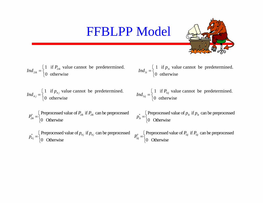
22


ikik

PInd

⎧= ⎨⎩

33


ii

pInd

⎧= ⎨⎩

44


jj

pInd

⎧= ⎨⎩

55


ijij

PInd

⎧= ⎨⎩

2 2*2


ik ikik

P PP

⎧= ⎨⎩

3 3*3


i ii

p pp

⎧=⎨⎩

4 4*4


j jj

p pp

⎧= ⎨⎩

5 5*5


ij ijij

P PP

⎧=⎨⎩

FFBLPP Model

Full Factorial Robust Algorithm

Lemma 2: The algorithm presented terminates in finite number of steps. After the algorithm terminated with , it has either detected infeasibility or has found an optimal robust solution to the original problem

0=ε

Now let see how this proposed algorithm work in the real problem.

Robust RPS Infrastructure for Television Recycle in GA

12 Municipal collection sites

9 Commercial processing sites (A)

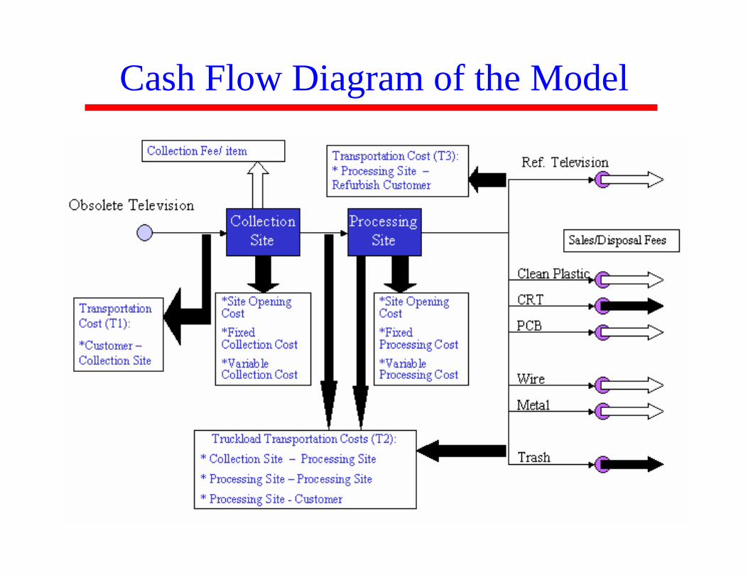
Cash Flow Diagram of the Model

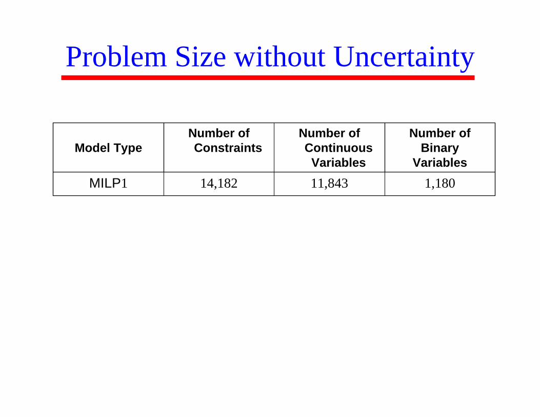
Problem Size without Uncertainty

1,18011,84314,182MILP1

Number of Binary

Variables

Number of Continuous Variables

Number of ConstraintsModel Type

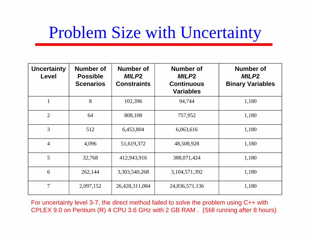
Problem Size with Uncertainty

1,18024,836,571,13626,428,311,0842,097,1527

1,1803,104,571,3923,303,540,268262,1446

1,180388,071,424412,943,91632,7685

1,18048,508,92851,619,3724,0964

1,1806,063,6166,453,8045123

1,180757,952808,108642

1,18094,744102,39681

Number of MILP2

Binary Variables

Number of MILP2

Continuous Variables

Number of MILP2

Constraints

Number of Possible

Scenarios

Uncertainty Level

For uncertainty level 3-7, the direct method failed to solve the problem using C++ with CPLEX 9.0 on Pentium (R) 4 CPU 3.6 GHz with 2 GB RAM . (Still running after 8 hours)

Performance of the Proposed Algorithm

N/A1,947.8953,864.330.0003%62,097,1527

N/A1,084.4352,100.330.0019%5262,1446

N/A1,909.9951,918.700.02%732,7685

N/A1,246.3646,756.290.15%64,0964

N/A516.2942,397.840.78%45123

15,504.51506.3042,397.846.25%4642

1,186.8858.505,244.7525%281

Time (sec)Direct Method

Time (sec)Proposed Algorithm

Min-Max Regret

Ratio Between # Scenarios Generated and Total # Scenarios

# Scenarios Generated

Total # Scenarios

Uncertainty Level

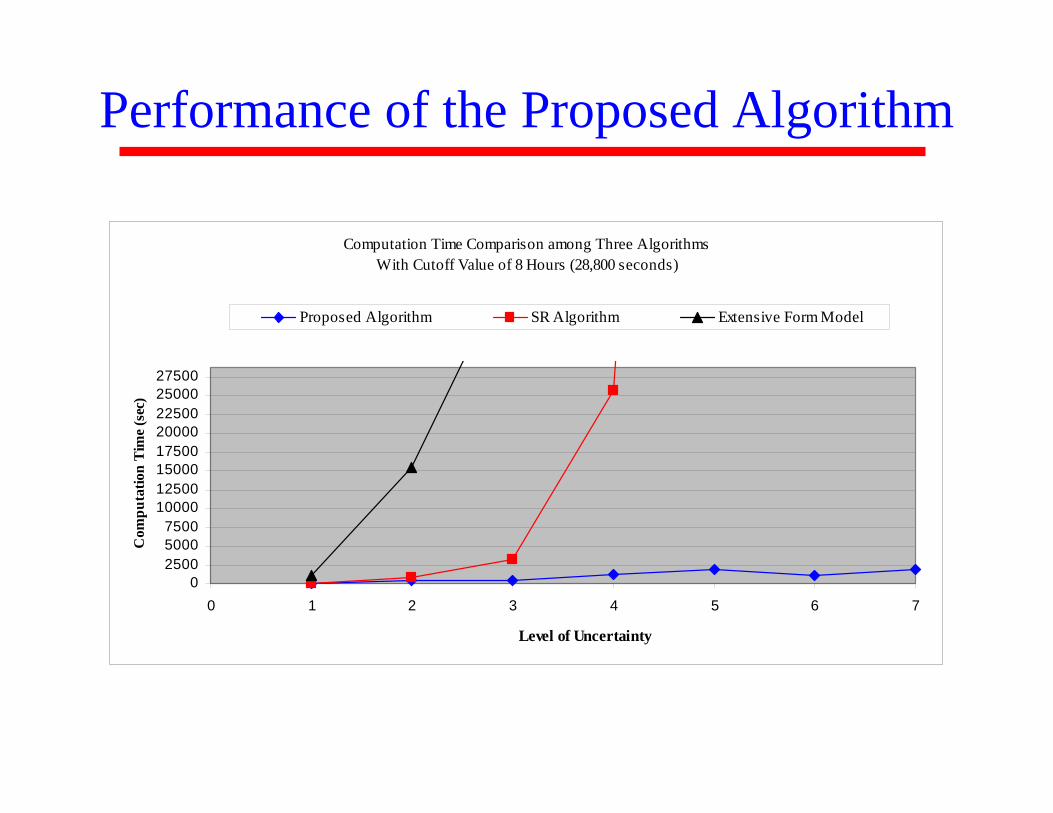
Performance of the Proposed Algorithm

Computation Time Comparison among Three AlgorithmsWith Cutoff Value of 8 Hours (28,800 seconds)

0250050007500

1000012500150001750020000225002500027500

0 1 2 3 4 5 6 7

Level of Uncertainty

Com

puta

tion

Tim

e (s

ec)

Proposed Algorithm SR Algorithm Extensive Form Model

Research Contribution

• Theoretical ContributionInnovative approaches to generate Min-Max regret robust solution when each uncertain parameter independentlytakes its value from a finite set of real values and the scenarios design is a full factorial design.

• Practical ContributionPractical approaches for large-scale robust planning problem under uncertainty.

Special Thanks

Dr. Matthew J. RealffChemical & Biomolecular Engineering

Dr. Jane C. AmmonsIndustrial & Systems Engineering

Questions

Please feel free to ask questions. I will do my best to answer all of them.

Thank you so much for coming to my presentation. Please have a wonderful day.

a new min-max regret robust optimization approach for ...nau/adversarial/program/posters/...kk k...

Documents