A NEW ALGORITHM FOR SENSORS VERIFICATION AND CORRECTION

IN AIR HANDLING UNITS

Nunzio Cotrufo, Radu Zmeureanu

Department of Building, Civil and Environmental Engineering

Concordia University

Montréal Quebec, Canada

ABSTRACT

The use of trend data from Building Automation

Systems (BAS) is a cost-effective strategy for ongoing

commissioning in HVAC systems. Quality of

measurements, thus, is essential for the effectiveness of

commissioning process. This paper presents an

approach to verify, and correct if necessary, the outdoor

air temperature and relative humidity measurements in

an AHU economizer. The proposed iterative algorithm

solves an optimization problem that maximizes the

goodness of fit, in terms of coefficient of variation, CV-

RMSE, between a directly measured variable, and its

value derived from an air energy balance. This approach

has been verified with data from an institutional

building in Montréal, proving its capability to highlight

errors in the measurements of outdoor air relative

humidity and temperature. Corrected values have been

finally validated through comparison against spot

measurements with calibrated sensors.

INTRODUCTION

The implementation of ongoing commissioning for

HVAC systems is a cost-effective strategy to overcome

the rise of faults and decrease in energy performance

over the entire building systems life cycle (Roth K. et

al., 2008). Faults and degradation can affect both

equipment and sensors, causing decrease in equipment

performance, energy wastes and occupancy discomfort.

This paper focuses on faulty sensors detection in Air

Handling Units (AHU), and presents a new algorithm to

automatically adjust the measured air temperature and

humidity. Faults in sensors may be often considered as

soft failures, and thus they may produce small persistent

waste of energy and/or discomfort for occupant, and

remaining unrevealed for a long time (Haves P., 1999).

Although numerous methods and algorithms for HVAC

Automatic Fault Detection and Diagnosis (AFDD) have

been developed during the last decades (Breuker M. S.

and J. E. Braun, 1998, Jia Y. and T. A. Reddy, 2003, Cui

J. and S. Wang, 2005), the same attention has not been

given to self-correction algorithms, making the human

intervention in commissioning strategies still crucial

(Padilla M. et al., 2015). Four different types of faults

are identified in sensors: bias faults, drift faults,

complete failures and precision degradation (Chen Y.

and L. Lan, 2010). Adding self-correction algorithms to

systems control codes allows to minimize fault effects

until the human action fix the fault (Fernandez N. et al.,

2009). Self-correction algorithms could consist of

virtual sensor measurements which replace values from

sensors detected as faulty. Several virtual sensors

algorithms have been developed for HVAC equipment

and components: Nassif et al. (2003), Song et al. (2012),

McDonald et al. (2014). Fernandez N. et al. (2009b)

presented algorithms for sensors fault detection,

isolation and correction in AHU. Algorithms implement

rules based on physical principles coupled with

knowledge of the AHU components configuration.

Brambley M. R. et al., 2011 presented a study on self-

correction strategies for AHU: 26 algorithms have been

based on models developed during commissioning in

order to simulate the correct system operation. Ten of

those algorithms were integrated in the code of a

prototype software for automated sensors fault detection

and correction. Padilla M. et al. (2015) proposed a

sensor correction algorithm for supply air temperature

and pressure in an AHU, developing grey box models

using variables usually measured for control purpose by

the Building Energy Management System (BEMS).

Whether a fault in sensors is detected, faulty

measurements are replaced by values derived from those

models. Finally, Padilla M. and D, Choiniere (2015)

developed an algorithm for sensors fault detection and

isolation in an AHU. The authors developed the

algorithm coupling Principal Component Analysis

(PCA) and Active Functional Tests (AFT). This paper presents a new algorithm for sensor self-

correction without need for human intervention or

additional measurements at additional cost. Results

from testing the algorithm in an AHU economizer are

presented as well.

ALGORTHM

The algorithm proposed in this paper aims for the self-

correction of measurements of outdoor air temperature

or relative humidity entering the AHU economizer.

Only one of these two sensors might show abnormal

measurements. Measurements from a BAS trend data

are used in this study. The reference value of outdoor air

temperature is predicted at each time step from the air

energy balance at the mixing box of the economizer

(assuming that all other sensors give accurate

measurements). The measurements are corrected with a

constant optimal value identified through an iterative

procedure, and compared with the correspondent

reference value. Short term measurements with

calibrated sensors are used for validation purpose only.

The algorithm could also be applied to the return or

mixed air stream, assuming as correct the measurements

from the other air temperature and relative humidity

sensors.

i) Energy Balance

The energy balance of mixing of two air streams in the

adiabatic mixing box of the AHU is written as presented

in Equation 1 in terms of α-factor. The α-factor is

intended as the ratio of the outdoor air flow rate to the

supply air flow rate (Eq. 2) (ASHRAE. 2001).

α = ℎ𝑚𝑎− ℎ𝑟𝑒𝑐

ℎ𝑜𝑎− ℎ𝑟𝑒𝑐 (1)

α = 𝑚𝑜𝑎

𝑚𝑎 (2)

where hma is the mixed air enthalpy, hrec is the

recirculated air enthalpy, and hoa is the outdoor air

enthalpy, moa is the outdoor air mass flow rate, and ma is

the supply air mass flow rate.

The outdoor air temperature entering the mixing box is

predicted from the energy balance in terms of α-factor

by using the sequence of Equations 3, 4 and 5 at each

time step.

𝑥𝑜𝑎,𝛼 = α·(𝑥𝑚𝑎 - 𝑥𝑟𝑒𝑐) + 𝑥𝑟𝑒𝑐 (3)

ℎ𝑜𝑎,𝛼 = α·(ℎ𝑚𝑎 - ℎ𝑟𝑒𝑐) + ℎ𝑟𝑒𝑐 (4)

𝑇𝑜𝑎,𝛼 = ℎ𝑜𝑎,𝛼− ℎ𝑓𝑔·𝑥𝑜𝑎,𝛼

𝐶𝑝𝑎+ 𝐶𝑝𝑣·𝑥𝑜𝑎,𝛼 (5)

where 𝑥𝑜𝑎,𝛼 is the outdoor air specific humidity

estimated with α-factor, kg/kg; 𝑥𝑚𝑎 is the mixed air

specific humidity, kg/kg; 𝑥𝑟𝑒𝑐 is the recirculated air

specific humidity, kg/kg; ℎ𝑜𝑎,𝛼 is the outdoor air

enthalpy estimated with α-factor, kJ/kg; 𝑇𝑜𝑎,𝛼 is the

outdoor air temperature estimated with α-factor, °C; ℎ𝑓𝑔

is the water vaporization heat, ℎ𝑓𝑔 = 2,501 kJ/kg; Cpv is

the water vapor specific heat at constant pressure P =

101,325 Pa; Cpv = 1,875 kJ/(kg K), and Cpa is the dry air

specific heat at constant pressure P = 101,325 Pa, Cpa =

1,006 kJ/(kg K).

Values derived from eq. 5 for each time step compose a

vector of temperatures, which are compared to the

outdoor air temperature measurements from the BAS.

The results of comparison are reported in terms of

Coefficient of Variation of the Root Mean Square Error

CV-RMSE (%). If high CV-RMSE values are obtained,

we conclude that the measurements of the variable of

interest (in this case the outdoor air temperature) might

contain abnormal values. We assume CV-RMSE values

higher than 10% to be indicative of the presence of

abnormal values. Investigation on the presented

algorithm using laboratory data should conducted in

order to identify an optimal CV-RMSE limit value for

abnormal values detection. In this case, the

measurements of outdoor air temperature need to be

corrected and, for this purpose, a self-correction

algorithm is proposed to be used. Certainly, the scope of

this correction should be limited in time until the

maintenance team make the physical corrections or

replacement of sensors.

ii) Iterative Procedure

The measured value of outdoor air temperature at each

time step is modified (Eq. 7). A delta vector (dT(j)) of

38 air temperature corrections, containing values from -

5.0°C up to +5.0°C, increased by 0.25°C, is used (Eq.

6). For each j-correction, a new α-factor vector of values

(αcor(j)) is derived through Equations 8 and 9.

dT = [-5.0, -4.75, -4.50 …. +4.50,+4.75, +5.0] (6)

𝑇𝑜𝑎,𝑐𝑜𝑟(𝑗) = 𝑇𝑜𝑎 + dT(j) (7)

ℎ𝑜𝑎,𝑐𝑜𝑟(𝑗) = Toa,cor(j)·Cpa +

+ 𝑥𝑜𝑎·(hgf + Toa,cor(j) ·Cpv)

(8)

αcor(j) = ℎ𝑚𝑎− ℎ𝑟𝑒𝑐

ℎ𝑜𝑎,𝑐𝑜𝑟(𝑗)− ℎ𝑟𝑒𝑐 (9)

where j varies from 1 to the 38, 𝑇𝑜𝑎,𝑐𝑜𝑟(j) is the j-th

corrected outdoor air temperature measurement,

ℎ𝑜𝑎,𝑐𝑜𝑟(𝑗) is the j-th corrected outdoor air enthalpy, and

αcor(j) is the j-th corrected α-factor. For each j, the

corrected vector of α-factor values is used with

equations 3, 4 and 5 to obtain a new predicted value of

Toa,α(j). For each j, the CV-RMSE between Toa, α (j) and

Toa,cor(j), over the entire sample, is calculated. The dT(j)

correction value that gives the minimum CV-RMSE is

retained as the best correction value dT(j*) of outdoor

air temperature.

Finally all measurements of outdoor air temperature Toa

recorded by the BAS are replaced with the corrected

outdoor air temperature Toa* (Eq. 10).

𝑇𝑜𝑎∗ = 𝑇𝑜𝑎 + dT(j*) (10)

In addition to the correction of measurements of the

outdoor air temperature, this iterative procedure allows

for the correction of α-factor. As a result, we obtain a

better estimate of the outdoor air flow rate, if there is no

air flow meter on the outdoor air intake. The

effectiveness of the overall algorithm is verified by

comparing the corrected outdoor air temperature

measurements with short term measurements with

calibrated sensors.

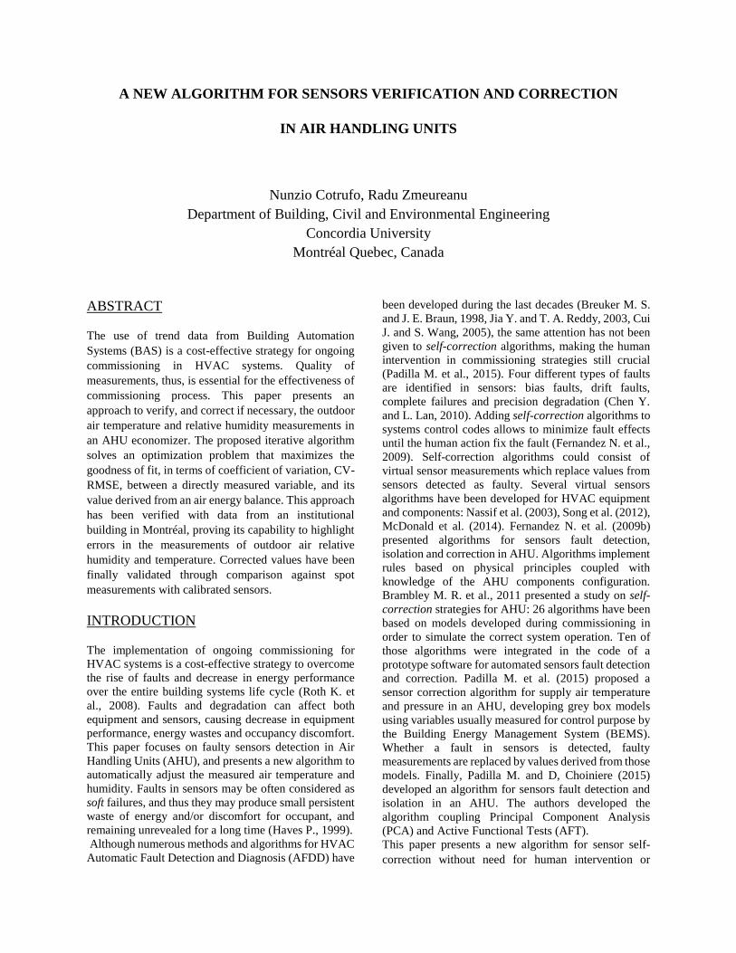
The flow-chart of the overall algorithm implementation

is showed in figure 1.

Figure 1 – Flow-chart of the overall algorithm process.

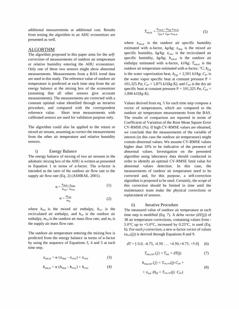
CASE STUDY This study uses two AHUs installed in parallel in a new

university building in Montréal, QC. The outdoor air

and recirculated air flows are mixed in two mixing

boxes, installed in parallel, before the air is treated and

supplied to the conditioned space (Figure 2). Four

variable speed fans are used to supply the conditioned

air to the building, and two fans for the returned air. Two

heat recovery coils are installed at the outdoor air intake

for pre-heating or pre-cooling.

Figure 2 – Schematic of the Air Handling Units.

The recirculated air temperature (Trec) and relative

humidity (RHrec), are derived from the return air

conditions, considering that the air specific humidity

does not change through the return fan, and the outdoor

air temperature increases by 1.8°C (Zibin N., 2014).

Table 1 lists variables used in this study from the BAS

trend data that contains measurements recorded at 15-

min time step.

Moreover, short term measurements with calibrated

sensors have been taken from September 2 to September

19 in 2015 in order to preliminary verify the accuracy of

measurements from the BAS. Short term measurements

of the mixed air relative humidity have been taken, since

this variable is not recorded by the BAS. Measurements

from BAS trend data taken when the heat recovery coils

were working have been excluded from the data set.

Table 1 – Variable used in this study for sensors

self-correction.

Variable Unit Symbol

Outdoor air temperature °C Toa

Outdoor air relative humidity

% RHoa

Return air temperature °C Tr

Return air relative humidity % RHr

Mixed air temperature °C Tma

Mixed air relative humidity % RHma

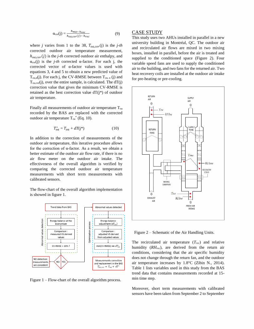
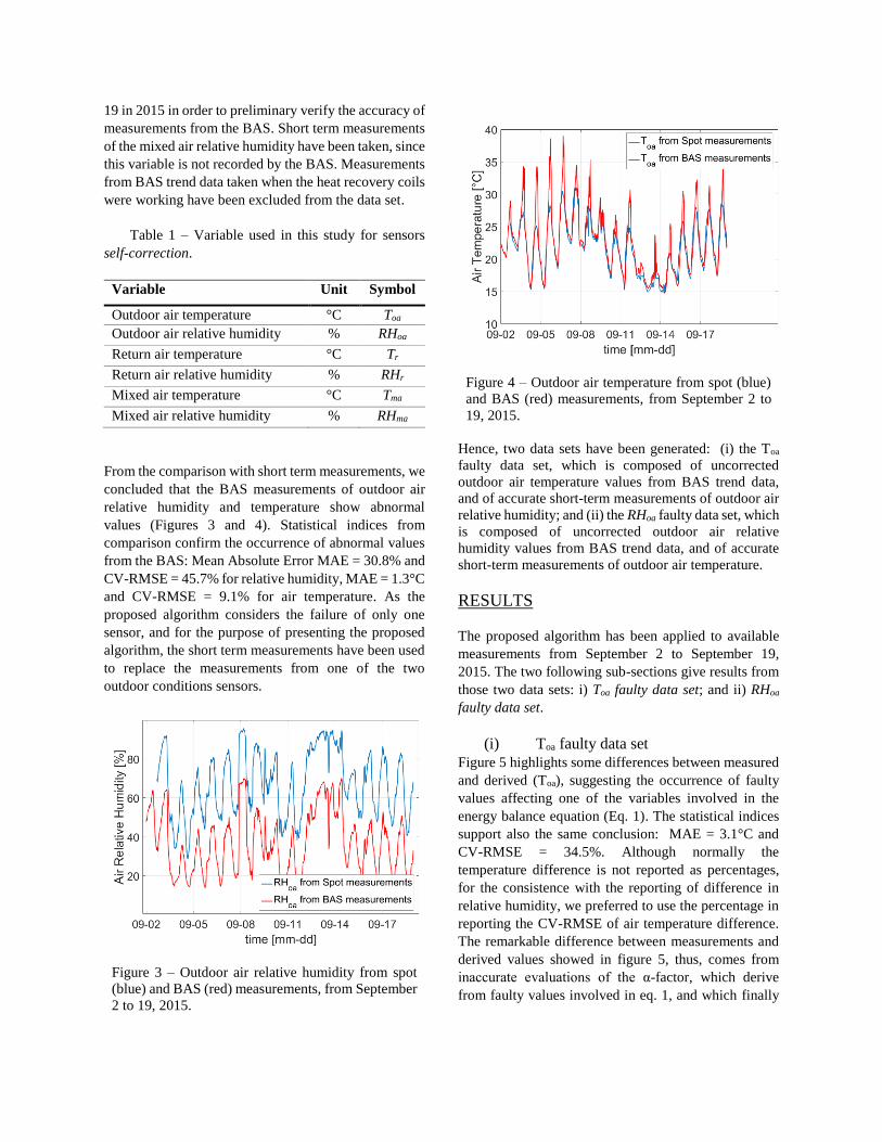
From the comparison with short term measurements, we

concluded that the BAS measurements of outdoor air

relative humidity and temperature show abnormal

values (Figures 3 and 4). Statistical indices from

comparison confirm the occurrence of abnormal values

from the BAS: Mean Absolute Error MAE = 30.8% and

CV-RMSE = 45.7% for relative humidity, MAE = 1.3°C

and CV-RMSE = 9.1% for air temperature. As the

proposed algorithm considers the failure of only one

sensor, and for the purpose of presenting the proposed

algorithm, the short term measurements have been used

to replace the measurements from one of the two

outdoor conditions sensors.

Figure 3 – Outdoor air relative humidity from spot

(blue) and BAS (red) measurements, from September

2 to 19, 2015.

Figure 4 – Outdoor air temperature from spot (blue)

and BAS (red) measurements, from September 2 to

19, 2015.

Hence, two data sets have been generated: (i) the Toa

faulty data set, which is composed of uncorrected

outdoor air temperature values from BAS trend data,

and of accurate short-term measurements of outdoor air

relative humidity; and (ii) the RHoa faulty data set, which

is composed of uncorrected outdoor air relative

humidity values from BAS trend data, and of accurate

short-term measurements of outdoor air temperature.

RESULTS

The proposed algorithm has been applied to available

measurements from September 2 to September 19,

2015. The two following sub-sections give results from

those two data sets: i) Toa faulty data set; and ii) RHoa

faulty data set.

(i) Toa faulty data set

Figure 5 highlights some differences between measured

and derived (Toa), suggesting the occurrence of faulty

values affecting one of the variables involved in the

energy balance equation (Eq. 1). The statistical indices

support also the same conclusion: MAE = 3.1°C and

CV-RMSE = 34.5%. Although normally the

temperature difference is not reported as percentages,

for the consistence with the reporting of difference in

relative humidity, we preferred to use the percentage in

reporting the CV-RMSE of air temperature difference.

The remarkable difference between measurements and

derived values showed in figure 5, thus, comes from

inaccurate evaluations of the α-factor, which derive

from faulty values involved in eq. 1, and which finally

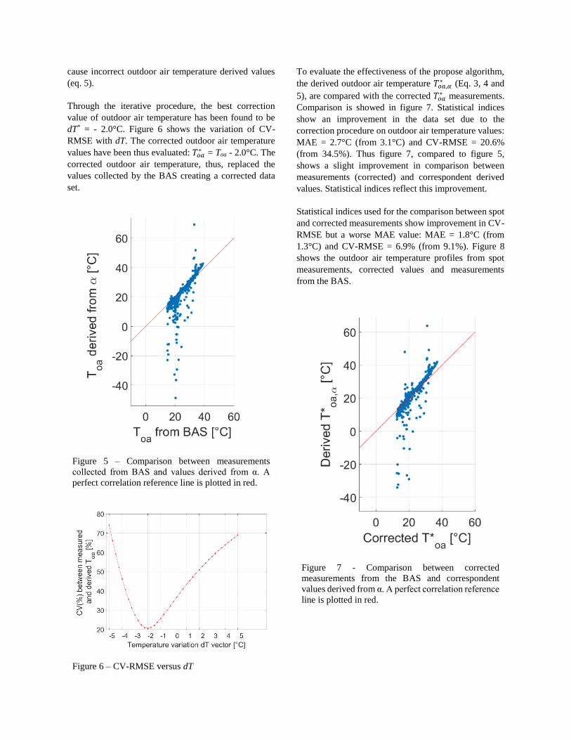
cause incorrect outdoor air temperature derived values

(eq. 5).

Through the iterative procedure, the best correction

value of outdoor air temperature has been found to be

dT* = - 2.0°C. Figure 6 shows the variation of CV-

RMSE with dT. The corrected outdoor air temperature

values have been thus evaluated: 𝑇𝑜𝑎∗ = Toa - 2.0°C. The

corrected outdoor air temperature, thus, replaced the

values collected by the BAS creating a corrected data

set.

Figure 5 – Comparison between measurements

collected from BAS and values derived from α. A

perfect correlation reference line is plotted in red.

Figure 6 – CV-RMSE versus dT

To evaluate the effectiveness of the propose algorithm,

the derived outdoor air temperature 𝑇𝑜𝑎,𝛼∗ (Eq. 3, 4 and

5), are compared with the corrected 𝑇𝑜𝑎∗ measurements.

Comparison is showed in figure 7. Statistical indices

show an improvement in the data set due to the

correction procedure on outdoor air temperature values:

MAE = 2.7°C (from 3.1°C) and CV-RMSE = 20.6%

(from 34.5%). Thus figure 7, compared to figure 5,

shows a slight improvement in comparison between

measurements (corrected) and correspondent derived

values. Statistical indices reflect this improvement.

Statistical indices used for the comparison between spot

and corrected measurements show improvement in CV-

RMSE but a worse MAE value: MAE = 1.8°C (from

1.3°C) and CV-RMSE = 6.9% (from 9.1%). Figure 8

shows the outdoor air temperature profiles from spot

measurements, corrected values and measurements

from the BAS.

Figure 7 - Comparison between corrected

measurements from the BAS and correspondent

values derived from α. A perfect correlation reference

line is plotted in red.

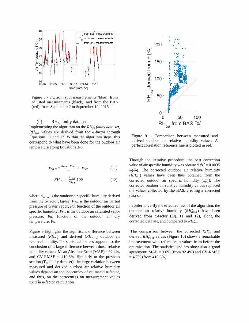
Figure 8 - Toa from spot measurements (blue), from

adjusted measurements (black), and from the BAS

(red), from September 2 to September 19, 2015.

(ii) RHoa faulty data set

Implementing the algorithm on the RHoa faulty data set,

RHoa,α values are derived from the α-factor through

Equations 11 and 12. Within the algorithm steps, this

correspond to what have been done for the outdoor air

temperature along Equations 3-5.

𝑥𝑜𝑎,𝛼 = 𝑥𝑚𝑎− 𝑥𝑟𝑒𝑐

𝛼+ 𝑥𝑟𝑒𝑐 (11)

RHoa,α = 𝑃𝑣𝑜𝑎

𝑃𝑠𝑜𝑎·100 (12)

where 𝑥𝑜𝑎,𝛼 is the outdoor air specific humidity derived

from the α-factor, kg/kg; Pvoa is the outdoor air partial

pressure of water vapor, Pa, function of the outdoor air

specific humidity; Psoa is the outdoor air saturated vapor

pressure, Pa, function of the outdoor air dry

temperature, Pa.

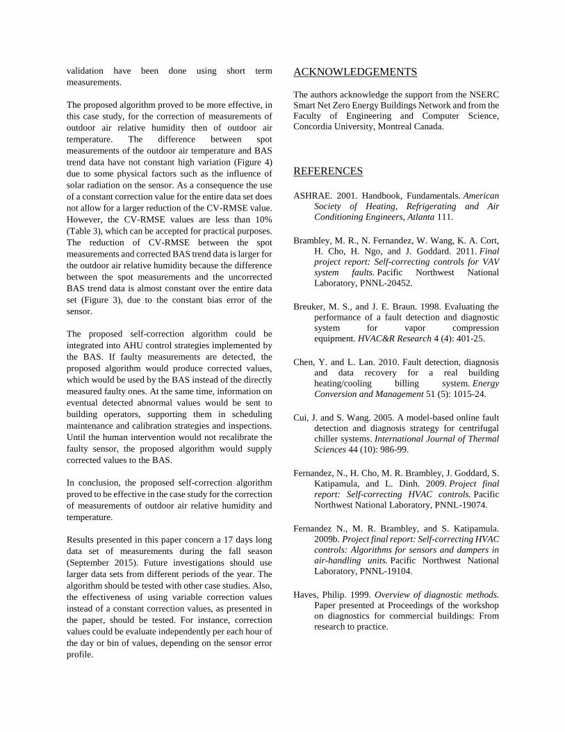
Figure 9 highlights the significant difference between

measured (RHoa) and derived (RHoa,α) outdoor air

relative humidity. The statistical indices support also the

conclusion of a large difference between those relative

humidity values: Mean Absolute Error (MAE) = 92.4%,

and CV-RMSE = 410.6%. Similarly to the previous

section (Toa faulty data set), the large variation between

measured and derived outdoor air relative humidity

values depend on the inaccuracy of estimated α-factor,

and thus, on the correctness on measurement values

used in α-factor calculation.

Figure 9 – Comparison between measured and

derived outdoor air relative humidity values. A

perfect correlation reference line is plotted in red.

Through the iterative procedure, the best correction

value of air specific humidity was obtained dx* = 0.0035

kg/kg. The corrected outdoor air relative humidity

(𝑅𝐻𝑜𝑎∗ ) values have been thus obtained from the

corrected outdoor air specific humidity (𝑥𝑜𝑎∗ ). The

corrected outdoor air relative humidity values replaced

the values collected by the BAS, creating a corrected

data set.

In order to verify the effectiveness of the algorithm, the

outdoor air relative humidity (𝑅𝐻𝑜𝑎,𝛼∗ ) have been

derived from α-factor (Eq. 11 and 12), along the

corrected data set, and compared to 𝑅𝐻𝑜𝑎∗ .

The comparison between the corrected 𝑅𝐻𝑜𝑎∗ and

derived 𝑅𝐻𝑜𝑎,𝛼∗ values (Figure 10) shows a remarkable

improvement with reference to values from before the

optimization. The statistical indices show also a good

agreement: MAE = 3.6% (from 92.4%) and CV-RMSE

= 4.7% (from 410.6%).

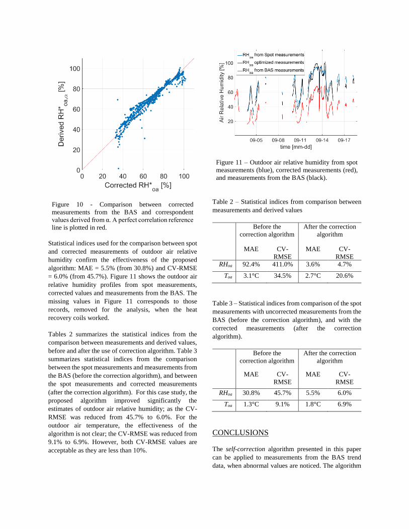
Figure 10 - Comparison between corrected

measurements from the BAS and correspondent

values derived from α. A perfect correlation reference

line is plotted in red.

Statistical indices used for the comparison between spot

and corrected measurements of outdoor air relative

humidity confirm the effectiveness of the proposed

algorithm: MAE = 5.5% (from 30.8%) and CV-RMSE

= 6.0% (from 45.7%). Figure 11 shows the outdoor air

relative humidity profiles from spot measurements,

corrected values and measurements from the BAS. The

missing values in Figure 11 corresponds to those

records, removed for the analysis, when the heat

recovery coils worked.

Tables 2 summarizes the statistical indices from the

comparison between measurements and derived values,

before and after the use of correction algorithm. Table 3

summarizes statistical indices from the comparison

between the spot measurements and measurements from

the BAS (before the correction algorithm), and between

the spot measurements and corrected measurements

(after the correction algorithm). For this case study, the

proposed algorithm improved significantly the

estimates of outdoor air relative humidity; as the CV-

RMSE was reduced from 45.7% to 6.0%. For the

outdoor air temperature, the effectiveness of the

algorithm is not clear; the CV-RMSE was reduced from

9.1% to 6.9%. However, both CV-RMSE values are

acceptable as they are less than 10%.

Figure 11 – Outdoor air relative humidity from spot

measurements (blue), corrected measurements (red),

and measurements from the BAS (black).

Table 2 – Statistical indices from comparison between

measurements and derived values

Before the

correction algorithm

After the correction

algorithm

MAE CV-

RMSE

MAE CV-

RMSE RHoa 92.4% 411.0% 3.6% 4.7%

Toa 3.1°C 34.5% 2.7°C 20.6%

Table 3 – Statistical indices from comparison of the spot

measurements with uncorrected measurements from the

BAS (before the correction algorithm), and with the

corrected measurements (after the correction

algorithm).

Before the

correction algorithm

After the correction

algorithm

MAE CV-

RMSE

MAE CV-

RMSE

RHoa 30.8% 45.7% 5.5% 6.0%

Toa 1.3°C 9.1% 1.8°C 6.9%

CONCLUSIONS

The self-correction algorithm presented in this paper

can be applied to measurements from the BAS trend

data, when abnormal values are noticed. The algorithm

validation have been done using short term

measurements.

The proposed algorithm proved to be more effective, in

this case study, for the correction of measurements of

outdoor air relative humidity then of outdoor air

temperature. The difference between spot

measurements of the outdoor air temperature and BAS

trend data have not constant high variation (Figure 4)

due to some physical factors such as the influence of

solar radiation on the sensor. As a consequence the use

of a constant correction value for the entire data set does

not allow for a larger reduction of the CV-RMSE value.

However, the CV-RMSE values are less than 10%

(Table 3), which can be accepted for practical purposes.

The reduction of CV-RMSE between the spot

measurements and corrected BAS trend data is larger for

the outdoor air relative humidity because the difference

between the spot measurements and the uncorrected

BAS trend data is almost constant over the entire data

set (Figure 3), due to the constant bias error of the

sensor.

The proposed self-correction algorithm could be

integrated into AHU control strategies implemented by

the BAS. If faulty measurements are detected, the

proposed algorithm would produce corrected values,

which would be used by the BAS instead of the directly

measured faulty ones. At the same time, information on

eventual detected abnormal values would be sent to

building operators, supporting them in scheduling

maintenance and calibration strategies and inspections.

Until the human intervention would not recalibrate the

faulty sensor, the proposed algorithm would supply

corrected values to the BAS.

In conclusion, the proposed self-correction algorithm

proved to be effective in the case study for the correction

of measurements of outdoor air relative humidity and

temperature.

Results presented in this paper concern a 17 days long

data set of measurements during the fall season

(September 2015). Future investigations should use

larger data sets from different periods of the year. The

algorithm should be tested with other case studies. Also,

the effectiveness of using variable correction values

instead of a constant correction values, as presented in

the paper, should be tested. For instance, correction

values could be evaluate independently per each hour of

the day or bin of values, depending on the sensor error

profile.

ACKNOWLEDGEMENTS

The authors acknowledge the support from the NSERC

Smart Net Zero Energy Buildings Network and from the

Faculty of Engineering and Computer Science,

Concordia University, Montreal Canada.

REFERENCES

ASHRAE. 2001. Handbook, Fundamentals. American

Society of Heating, Refrigerating and Air

Conditioning Engineers, Atlanta 111.

Brambley, M. R., N. Fernandez, W. Wang, K. A. Cort,

H. Cho, H. Ngo, and J. Goddard. 2011. Final

project report: Self-correcting controls for VAV

system faults. Pacific Northwest National

Laboratory, PNNL-20452.

Breuker, M. S., and J. E. Braun. 1998. Evaluating the

performance of a fault detection and diagnostic

system for vapor compression

equipment. HVAC&R Research 4 (4): 401-25.

Chen, Y. and L. Lan. 2010. Fault detection, diagnosis

and data recovery for a real building

heating/cooling billing system. Energy

Conversion and Management 51 (5): 1015-24.

Cui, J. and S. Wang. 2005. A model-based online fault

detection and diagnosis strategy for centrifugal

chiller systems. International Journal of Thermal

Sciences 44 (10): 986-99.

Fernandez, N., H. Cho, M. R. Brambley, J. Goddard, S.

Katipamula, and L. Dinh. 2009. Project final

report: Self-correcting HVAC controls. Pacific

Northwest National Laboratory, PNNL-19074.

Fernandez N., M. R. Brambley, and S. Katipamula.

2009b. Project final report: Self-correcting HVAC

controls: Algorithms for sensors and dampers in

air-handling units. Pacific Northwest National

Laboratory, PNNL-19104.

Haves, Philip. 1999. Overview of diagnostic methods.

Paper presented at Proceedings of the workshop

on diagnostics for commercial buildings: From

research to practice.

Jia Y. and T. A. Reddy. 2003. Characteristic physical

parameter approach to modeling chillers suitable

for fault detection, diagnosis, and

evaluation. Journal of Solar Energy

Engineering 125 (3): 258-65.

McDonald, E., R. Zmeureanu, and D. Giguère. 2013.

Virtual flow meter for chilled water loops in

existing buildings. ASHRAE Transactions; 2014,

120(2).

Nassif, N., S. Kajl, and R. Sabourin. 2003. Modélisation

des composants d'un système CVAC existant. In

VIe Colloque Interuniversitaire Franco-

Québécois, Québec, Canada. CIFQ2003 / 12-01.

Padilla, M., D. Choinière, and J. A. Candanedo. 2015. A

model-based strategy for self-correction of sensor

faults in VAV air handling units. Science and

Technology for the Built Environment.

Padilla M. and D. Choinière. 2015. A combined passive-

active sensor fault detection and isolation

approach for air handling units. Energy and

Buildings 99: 214-9.

Roth K., D. Westphalen, and J. Brodrick. 2008. Ongoing

commissioning. ASHRAE Journal 50 (3): 66.

Song, L., I. Joo, & G. Wang. 2012. Uncertainty analysis

of a virtual water flow measurement in building

energy consumption monitoring. HVAC&R

Research, 15:5, 997-1010.

Zibin N. 2014. A bottom-up method to calibrate

building energy models using building automation

system (BAS) trend data. Msc Degree., Concordia

University.