a method for estimating peak and time of peak … · a method for estimating peak and time of peak...
TRANSCRIPT

US Department of the InteriorUS Geological Survey
Scientific Investigations Report 2011ndash5104
Prepared in cooperation with the Harris County Flood Control District and the Texas Department of Transportation
A Method for Estimating Peak and Time of Peak Streamflow from Excess Rainfall for 10- to 640-Acre Watersheds in the Houston Texas Metropolitan Area
Cover Photograph courtesy of Steve Fitzgerald Harris County Flood Control District 2005
A Method for Estimating Peak and Time of Peak Streamflow from Excess Rainfall for 10- to 640-Acre Watersheds in the Houston Texas Metropolitan Area
By William H Asquith Theodore G Cleveland and Meghan C Roussel
Prepared in cooperation with the Harris County Flood Control District and the Texas Department of Transportation
Scientific Investigations Report 2011ndash5104
US Department of the Interior US Geological Survey
US Department of the Interior KEN SALAZAR Secretary
US Geological Survey Marcia K McNutt Director
US Geological Survey Reston Virginia 2011
For more information on the USGSmdashthe Federal source for science about the Earth its natural and living resources natural hazards and the environment visit httpwwwusgsgov or call 1-888-ASK-USGS
For an overview of USGS information products including maps imagery and publications visit httpwwwusgsgovpubprod
To order this and other USGS information products visit httpstoreusgsgov
Any use of trade product or firm names is for descriptive purposes only and does not imply endorsement by the US Government
Although this report is in the public domain permission must be secured from the individual copyright owners to reproduce any copyrighted materials contained within this report
Suggested citation Asquith WH Cleveland TG and Roussel MC 2011 A method for estimating peak and time of peak streamflow from excess rainfall for 10- to 640-acre watersheds in the Houston Texas metropolitan area US Geological Survey Scientific Investigations Report 2011ndash5104 41 p at httppubsusgsgovsir20115104
iii
Contents
Abstract 1 Introduction 1
Purpose and Scope 2 Study Watersheds 2
Database of Rainfall and Runoff 2 Selected Watershed Characteristics 5
Analysis of Gamma Unit Hydrographs for the 24 Watersheds 5 Background 5 Analysis 5 Computing Gamma Unit Hydrographs 11
Analysis of Rational Method for the 24 Watersheds 11 Background and Mathematical Analysis 11 Computational and Statistical Analysis 14
A Method for Estimating Peak and Time of Peak Streamflow from Excess Rainfall for 10- to 640-Acre Watersheds in the Houston Texas Metropolitan Area 17
Comparison of Results from Unit Hydrograph and Rational Method Analysis 17 Nomograph and Example Computations for the Method 21
Nomograph for the Method 21 Example Computations 21
Potential Bias in the Excess Rational Method 23 On the Relative Influence of Basin-Development Factor on Peak Streamflow 23
Influence of Basin-Development Factor 23 Example Computations 25
Summary 25 References 26 Glossary 29
Appendix 1mdashBasin-Development Factor 33 Appendix 2mdashSelected Unit Conversions 39
Figures
1 Map showing downstream locations of the 24 selected watersheds in the Houston Texas metropolishytan area used for gamma unit hydrograph and rational method analysis 3
2 Example of headers (definitions) and selected data parts of rainfall and runoff data files for storm on January 22 2006 for BMP Basin 504 on Armand Bayou Houston Texas 7
3 Statistical summary of watershed-specific peak streamflow of gamma unit hydrograph and regresshysion equation for estimation of peak streamflow for applicable watersheds in the Houston Texas metropolitan area 9
iv
4 Statistical summary of watershed-specific time to peak of gamma unit hydrograph and regression equation for estimation of time to peak for applicable watersheds in the Houston Texas metropolitan area 9
5 Statistical summary of watershed-specific gamma unit hydrograph shape parameter and regresshysion equation for estimation of shape parameter for applicable watersheds in the Houston Texas metropolitan area 9
6ndash9 Graphs showing
6 Relation between watershed-specific peak streamflow and fitted values of peak streamflow by regression shown in equation 5 for a gamma unit hydrograph developed for 24 watersheds in the Houston Texas metropolitan area 10
7 Relation between watershed-specific time to peak and fitted values of time to peak by regresshysion shown in equation 6 for a gamma unit hydrograph developed for 24 watersheds in the Houston Texas metropolitan area 10
8 Dimensionless gamma hydrographs by shape parameter for 24 watersheds in the Houston Texas metropolitan area and for applicable developed and undeveloped non-Houston watersheds 12
9 Example of a gamma unit hydrograph with a shape factor of 1 from a 05-square mile watershyshed with a basin-development factor of 9 12
10 Screenshot of highly specialized single-purpose software for inversion of rational method for storm on January 22 2006 for BMP Basin 504 on Armand Bayou Houston Texas 15
11 Screenshot of output from highly specialized single-purpose software showing computational results for storm on January 22 2006 for BMP Basin 504 on Armand Bayou Houston Texas as shown in figure 10 16
12 Statistical summary of watershed-specific runoff and volumetric runoff coefficients and runoff coefficient ratios for 24 watersheds in the Houston Texas metropolitan area 18
13 Statistical summary of watershed-specific time-R and regression equation for time-R estimation for applicable watersheds in the Houston Texas metropolitan area 18
14ndash16 Graphs showing
14 Relation between watershed-specific time-R and fitted values of time-R by regression shown in equation 19 developed for 24 watersheds in the Houston Texas metropolitan area 19
15 Relation between time to peak or depth of peak streamflow of the gamma unit hydrograph to drainage area and basin development factor 20
16 Nomograph of the relation between arithmetic means of peak and time of peak streamflow by gamma unit hydrograph and excess rational method computations for 1 inch of excess rainfall by selected basin-development factor and drainage area for 24 watersheds in the Houston Texas metropolitan area 22
17 Steps for implementing the method for 10- to 640-acre watersheds in the Houston Texas metropolishytan area 24
18 Graph showing relation between ratio of watershed-specific (mean) values of runoff coefficient and volumetric runoff coefficient to drainage area for 24 watersheds in the Houston Texas metropolitan area 24
Tables
1 Summary of 24 selected watersheds in the Houston Texas metropolitan area used for gamma unit hydrograph and rational method analysis 4
v
2 Summary of storm counts and watershed-mean parameters of gamma unit hydrograph analysis and watershed-mean parameters for rational method analysis of 24 selected watersheds in the Houston Texas metropolitan area 6
3 Comparison of values of peak and time of peak streamflow by gamma unit hydrograph and excess rational method computations for 1 inch of excess rainfall for limiting developed and undeveloped conditions for a 300-acre watershed in the Houston Texas metropolitan area 23
Conversion Factors
Multiply By To obtain
Length inch (in) 254 millimeter (mm) foot (ft) 3048 meter (m) mile (mi) 1609 kilometer (km)
Area square mile (mi2) 2590 square kilometer (km2) acre (acre) 001563 square mile (mi2) acre (acre) 004047 square kilometer (km2)
Flow cubic foot per second (ft3s) 02832 cubic meter per second (m3s)
Datum
Horizontal coordinate information is referenced to the North American Datum of 1983 (NAD 83) Vertical coordinate information is referenced to the North American Vertical Datum of 1988 (NAVD 88)
A Method for Estimating Peak and Time of Peak Streamflow from Excess Rainfall for 10- to 640-Acre Watersheds in the Houston Texas Metropolitan Area
By William H Asquith Theodore G Cleveland and Meghan C Roussel
Abstract
Estimates of peak and time of peak streamflow for small watersheds (less than about 640 acres) in a suburban to urban low-slope setting are needed for drainage design that is cost-effective and risk-mitigated During 2007ndash10 the US Geological Survey (USGS) in cooperation with the Harris County Flood Control District and the Texas Department of Transportation developed a method to estimate peak and time of peak streamflow from excess rainfall for 10- to 640-acre watersheds in the Houston Texas metropolitan area To develop the method 24 watersheds in the study area with drainage areas less than about 35 square miles (2240 acres) and with concomishytant rainfall and runoff data were selected The method is based on conjunctive analysis of rainfall and runoff data in the context of the unit hydrograph method and the ratioshynal method For the unit hydrograph analysis a gamma distribution model of unit hydrograph shape (a gamma unit hydrograph) was chosen and parameters estimated through matching of modeled peak and time of peak streamflow to observed values on a storm-by-storm basis Watershed mean or watershed-specific values of peak and time to peak (ldquotime to peakrdquo is a parameter of the gamma unit hydrograph and is distinct from ldquotime of peakrdquo) of the gamma unit hydrograph were computed Two regresshysion equations to estimate peak and time to peak of the gamma unit hydrograph that are based on watershed charshyacteristics of drainage area and basin-development factor (BDF) were developed For the rational method analysis a lag time (time-R) volumetric runoff coefficient and runoff coefficient were computed on a storm-by-storm basis Watershed-specific values of these three metrics were computed A regression equation to estimate time-R based on drainage area and BDF was developed Overall arithmetic means of volumetric runoff coefficient (041 dimensionless) and runoff coefficient (025 dimensionless)
for the 24 watersheds were used to express the rational method in terms of excess rainfall (the excess rational method) Both the unit hydrograph method and excess rational method are shown to provide similar estimates of peak and time of peak streamflow The results from the two methods can be combined by using arithmetic means A nomograph is provided that shows the respecshytive relations between the arithmetic-mean peak and time of peak streamflow to drainage areas ranging from 10 to 640 acres The nomograph also shows the respective relashytions for selected BDF ranging from undeveloped to fully developed conditions The nomograph represents the peak streamflow for 1 inch of excess rainfall based on drainage area and BDF the peak streamflow for design storms from the nomograph can be multiplied by the excess rainshyfall to estimate peak streamflow Time of peak streamflow is readily obtained from the nomograph Therefore given excess rainfall values derived from watershed-loss modshyels which are beyond the scope of this report the nomoshygraph represents a method for estimating peak and time of peak streamflow for applicable watersheds in the Houston metropolitan area Lastly analysis of the relative influence of BDF on peak streamflow is provided and the results indicate a 004log10 cubic feet per second change of peak streamflow per positive unit of change in BDF This relshyative change can be used to adjust peak streamflow from the method or other hydrologic methods for a given BDF to other BDF values example computations are provided
Introduction
Estimation of peak and time of peak streamflow from design storms provides for cost-effective risk-mitigated design of drainage structures such as bridges culverts roadways and other infrastructure Relevant guidelines or manuals which provide further context related to infrasshy
2 A Method for Estimating Peak and Time of Peak Streamflow for 10- to 640-Acre Watersheds in Houston Texas
tructure design can be found in Texas Department of Transportation (2002) or Harris County Flood Control District (2004)
Accordingly during 2007ndash10 the US Geological Survey (USGS) in cooperation with the Harris County Flood Control District (HCFCD) and the Texas Departshyment of Transportation (TxDOT) developed a method for estimating peak and time of peak streamflow from excess rainfall for 10- to 640-acre watersheds in the Houston Texas metropolitan area
Purpose and Scope
The primary purpose of this report is to present a method for estimating peak and time of peak stream-flow from excess rainfall for 10- to 640-acre watersheds in the Houston Texas metropolitan area that is based on watershed characteristics of drainage area and basin-development factor A secondary purpose is to report on the conjunctive analysis of rainfall and runoff data in the context of the unit hydrograph and the rational method for 24 watersheds in the Houston metropolitan area There are three major components of this report
1 A comprehensive summary of the unit hydrograph method and statistical results from analysis for the 24 watersheds is provided in the section titled ldquoAnalshyysis of Gamma Unit Hydrographs for the 24 Watershyshedsrdquo The section documents two equations that parameterize a gamma unit hydrograph and each is used in the development of the method described in
component 3
2 A comprehensive summary of the rational method and statistical results from analysis for the 24 watershysheds is provided in the section titled ldquoAnalysis of Rational Method for the 24 Watershedsrdquo The section documents an equation and appropriate runoff coefshyficient values which are used in the development of the method described in component 3
3 The method is based on conjunctive analysis of rainshyfall and runoff data in the context of the unit hydro-graph and the rational method for the watersheds and is presented in section titled ldquoA Method for Estimatshying Peak and Time of Peak Streamflow from Excess Rainfall for 10- to 640-Acre Watersheds in the Housshyton Texas Metropolitan Areardquo The primary result of the conjunctive analysis is a nomograph Examshyple computations involving the nomograph also are provided
Study Watersheds
For this investigation 21 distinct watersheds (based on latitude and longitude) were identified as pertinent for the Houston metropolitan area Pertinent watersheds were selected on the basis of drainage area as a measure of watershed size These watersheds represent genershyally the smallest watersheds for which there exist paired rainfall and runoff data suitable for conjunctive analysis of the unit hydrograph method and the rational method Although the focus of the investigation is the unit hydro-graph method and the rational method in the context of small watersheds (less than about 640 acres) to supshyport statistical development watersheds with drainage areas less than about 35 square miles (2240 acres) were selected
Two of the watersheds were identified as having considerable changes in extent of land development as expressed by a basin-development factor The period of record for the two watersheds was thus segregated (three total divisions) resulting in the 24 watersheds that are used in this report The 24 watersheds and ancillary charshyacteristics are listed in table 1 and shown in figure 1 Colshylectively these 24 watersheds are assumed to represent the generalized hydrologic and hydraulic conditions of many small low-slope watersheds in the Houston metropolitan area
Database of Rainfall and Runoff A database of rainfall and runoff data from about
1965 through about 2006 for the 24 watersheds was comshypiled and converted to digital format as needed The data for the 24 watersheds were obtained from various sources including Liscum and others (1996) and Liscum (2001) and from selected non-USGS rainfall-runoff data (Fred Liscum PBSampJ Inc [now (2011) with HCFCD] written commun 2008 and Steve Johnson LJA Engineering Inc written commun 2008) These collective data used here are stored in files available from the Texas Water Science Center upon request
An example of headers (definitions) and selected data parts of two data files for a selected storm for one of the study watersheds is shown in figure 2 The definitions in the figure are identical to those described in Asquith Thompson and others (2004 p 11 and 17) For the rainshyfall data the time stamps which are evenly spaced in the example (but not universally in the data) are shown under the DATE_TIME field The cumulative depth of weighted (WTD) rainfall among all available rain gages is available under the ACCUM_WTD_PRECIP field in units of inches For the parshyticular example a single rain gage (PRECIP1) was operated
Introduction 3
Figure 1 Map showing downstream locations of the 24 selected watersheds in the Houston Texas metropolitan area used for gamma unit hydrograph and rational method analysis
TheWoodlands
Houston
sectbrvbar610
sectbrvbar45
sectbrvbar10
sectbrvbar45
sectbrvbar45
poundcurren90poundcurren290
poundcurren90
poundcurren59
UV8
UV6
UV288
UV494
UV548
UV225
UV527
UV261
UV8
UV8
HARRIS COUNTY
MONTGOMERYCOUNTY
FORT BEND COUNTY
LIBERTY
CO
UN
TY
BRAZORIACOUNTY
LakeHouston
Brickhouse Gully
Berry BayouG
reensBayou
Armand
Bayou
Hunting Bayou
9
8 and 19
6 and 7
4
3
2
1
24
23
22
20
18
16
15
14
13
10 11 and 12
21
5
17
0 5 75
75
25
0 525
95deg1595deg30
30deg00
29deg45
24
EXPLANATION
Downstream location of watershedand sequence number (table 1)
TEXAS
Mapboundary
4 A Method for Estimating Peak and Time of Peak Streamflow for 10- to 640-Acre Watersheds in Houston Texas
Table 1 Summary of 24 selected watersheds in the Houston Texas metropolitan area used for gamma unit hydrograph and rational method analysis
[ no number fig figure A drainage area (contributing) L main-channel length S dimensionless main-channel slope BDF basin-development factor -- not available St Street Dr Drive trib tributary BMP Best-management practice Pkwy Parkway Rd Road NPDES National Pollutant Discharge Elimination System ]
Site no used in
fig 1
Station no and calendar year
range of storms Station name Latitude Longitude
A (square miles)
L (miles)
S (dimenshy
sionshyless)
BDF (dimenshy
sionshyless)
1 08068438 1975ndash87 Swale no 8 at Woodlands Tex 30deg0838 95deg2809 055 074 00077 8 2 08073630 1979ndash85 Bettina St Ditch Houston Tex 29deg4632 95deg3223 137 73 0041 11 3 08073750 1967ndash72 Stoney Brook St Ditch Houston Tex 29deg4405 95deg3022 50 -shy -shy 10 4 08073800 1964ndash72 Bering Ditch at Woodway Dr Houston 29deg4522 95deg2944 277 135 0019 9
Tex 5 08074145 1980ndash82 Bingle Rd storm sewer Houston Tex 29deg5131 95deg2909 21 70 0011 9 6 08074200 1965ndash75 Brickhouse Gully at Clarblak St Housshy 29deg4953 95deg3142 256 85 0030 3
ton Tex 7 08074200 1978ndash84 Brickhouse Gully at Clarblak St Housshy 29deg4953 95deg3142 256 85 0030 6
ton Tex 8 08074400 1980ndash82 Lazybrook St storm sewer Houston 29deg4815 95deg2604 13 69 0047 12
Tex 9 08074910 1979ndash83 Hummingbird St Ditch Houston Tex 29deg3944 95deg2911 32 145 0008 9
10 08075550 1966ndash72 Berry Bayou at Gilpin St Houston 29deg3832 95deg1322 326 334 0018 5 Tex
11 08075550 1974ndash78 Berry Bayou at Gilpin St Houston 29deg3832 95deg1322 287 334 0018 7 Tex
12 08075550 1979ndash84 Berry Bayou at Gilpin St Houston 29deg3832 95deg1322 256 334 0018 7 Tex
13 08075600 1965ndash72 Berry Bayou trib at Globe St Housshy 29deg3900 95deg1418 158 227 0017 5 ton Tex
14 08075750 1965ndash72 Hunting Bayou trib at Cavalcade St 29deg4800 95deg2002 120 178 0013 4 Houston Tex
15 00000BW8 2004ndash06 BMP Beltway 8 mitigation bank near 29deg5554 95deg1229 14 -shy -shy 11 Greens Bayou Houston Tex
16 0000B504 2005ndash06 BMP Basin 504 on Armand Bayou 29deg3628 95deg0655 19 103 0010 9 Houston Tex
17 0000K542 2005ndash06 BMP K542 Eldridge Pkwy at Louetta 30deg0015 95deg3723 18 81 0010 12 Rd Houston Tex
18 011NS004 2004ndash06 NPDES 011NS004 West 11th St Housshy 29deg4721 95deg2558 36 -shy -shy 9 ton Tex
19 0LBNS001 2000ndash02 NPDES 0LBNS001 Lazybrook storm 29deg4815 95deg2604 10 -shy -shy 12 sewer at White Oak Bayou Houston Tex
20 0TGNS002 2000ndash02 NPDES 0TGNS002 Tanglewilde at 29deg4436 95deg3204 06 -shy -shy 12 Houston Tex
21 0WBNS003 2004ndash05 NPDES 0WBNS003 Willowbrook Mall 29deg5725 95deg3217 13 -shy -shy 12 near Greens Rd Houston Tex
22 X8068420 1985ndash1986 Ditch C at Wedgewood Lake Woodshy 30deg1000 95deg2910 33 93 0041 0 lands Tex
23 X8068426 1985ndash1986 Ditch A at Woodlands Parkway Woodshy 30deg0900 95deg2930 41 16 0030 7 lands Tex
24 0BFDN000 1992 Briar Forest Dr storm sewer at Housshy 29deg4521 95deg3759 07 -shy -shy 4 ton Tex
5 Analysis of Gamma Unit Hydrographs for the 24 Watersheds
For other storms or watersheds two or more rain gages might have been operated and these data also are availshyable within the database The rainfall used for data proshycessing herein is always provided in the ACCUM_WTD_PRECIP
field For the runoff data the time stamps which also are
evenly spaced in the example but not universally in the database are shown under the DATE_TIME field The time stamps within the separate rainfall and runoff data files for the same storm might not have a one-to-one corresponshydence The streamflow in cubic feet per second is listed under the RUNOFF field The cumulative volume of runoff in inches is provided in the ACCUM_RUNOFF field
Selected Watershed Characteristics
Selected characteristics for the 24 watersheds were obtained from various sources including Liscum and others (1996) and from colleagues (Duane Barrett RG Miller Engineers Inc Fred Liscum PBSampJ Inc [now (2011) with HCFCD] and Steve Johnson LJA Engishyneering Inc written commun 2008) The characterisshytics include drainage area (contributing) main-channel length dimensionless main-channel slope and basin-development factor
1 Values for drainage area (contributing) A for each watershed were obtained and are listed in table 1
2 Values for main-channel length L were obtained and are listed in table 1 The L is defined as the length in stream-course miles of the longest defined chanshynel from the approximate watershed headwaters to the outlet There is considerable ambiguity in estishymation of L in the Houston metropolitan area where small watersheds can contain interconnected chanshynels ditches streets and storm sewers As a result some lengths could not be precisely quantified and are not listed in table 1
3 Values for dimensionless main-channel slope S (feet per feet) were obtained and are listed in table 1 The S is defined as the change in elevation ΔE in feet between the two end points of L divided by L in feet S = ΔE(5280 times L) Because of the ambiguity in estimation of L some slopes could not be precisely quantified and are not listed in table 1
4 Values for the dimensionless basin-development factor BDF were obtained and are listed in table 1 BDFs are integers from 0 to 12 There are 13 BDF categories resulting in 12 discrete changes in BDF from 0 rarr 1 1 rarr 2 and so forth through 11 rarr 12
BDF as a concept and definition for this report is described in appendix 1
Analysis of Gamma Unit Hydrographs for the 24 Watersheds
Background
The unit hydrograph method (Dingman 2002) estishymates the runoff hydrograph given an excess rainfall hyetograph Excess rainfall is a volume of rainfall per unit area (depth) after watershed losses such as evaporation infiltration and depression storage are subtracted (Chow and others 1988 p 135) A unit hydrograph is defined as the runoff hydrograph that results from a unit pulse of excess rainfall uniformly distributed over a watershed at a constant rate for a specific duration (Chow and others 1988 p 213)
Extensive investigations of the unit hydrograph method with Texas data and gamma distributions as the form of the unit hydrograph (Haan and others 1994 p 79) are available in Asquith and others (2005) and Asquith and Roussel (2007) In an associated study Cleveshyland and others (2006) documented an independent analshyysis of unit hydrographs for Texas A gamma distribution form of the unit hydrograph is referred to as a gamma unit hydrograph For this report an analysis of gamma unit hydrographs for the 24 watersheds was made Results of the gamma unit hydrograph analysis are listed in table 2 (columns 2ndash5)
Analysis
In total 317 data files were considered for the 24 watersheds The number of storms (discrete peaks) analyzed per watershed and per methods of this report is listed in table 2 These numbers were not used as weights in statistical computations such as weight factors in weighted-least squares regression because of the absence of numerical similarity in the ldquoNo of storms rdquo (three separate columns) between the USGS monitored watershysheds (the first 14 entries in the table) and the remaining watersheds
For each watershed unit hydrographs were generated from the rainfall and runoff data by using a custom modshyeling technique developed for Asquith and others (2005) Asquith and Roussel (2007) The technique involved an analyst-directed approach for 5-minute gamma unit hydro-graph estimation The output consisted of graphics (not
6 A Method for Estimating Peak and Time of Peak Streamflow for 10- to 640-Acre Watersheds in Houston Texas
Table 2 Summary of storm counts and watershed-mean parameters of gamma unit hydrograph analysis and watershed-mean parameters for rational method analysis of 24 selected watersheds in the Houston Texas metropolitan area
[ no number GUH gamma unit hydrograph analysis qp peak streamflow Tp time to peak K gamma hydrograph shape Cv volumetric runoff coefficient Cr runoff coefficient Tc time of concentration ]
Station no and calendar year
range of storms
No of storms for GUH
qp (inches
per hour)
Tp (hours)
K (dimenshy
sionshyless)
No of storms for Cv
No of storms for Cr
Tc (hours)
Cv (dimenshy
sionshyless)
Cr (dimenshy
sionshyless)
08068438 1975ndash87 11 04602 09091 12529 15 15 12625 05862 03521
08073630 1979ndash85 21 4935 8333 12157 25 25 12952 5494 3650
08073750 1967ndash72 12 5242 2847 2439 14 14 6095 4866 3789
08073800 1964ndash72 26 3450 5641 3580 18 15 21211 6398 4225
08074145 1980ndash82 20 16242 5083 44461 35 35 4809 5250 4944
08074200 1965ndash75 18 1537 23610 9768 19 17 44618 3531 0968
08074200 1978ndash84 21 1991 9048 3193 32 30 18834 3446 1761
08074400 1980ndash82 22 23764 1288 7315 29 29 2550 4544 4757
08074910 1979ndash83 14 5224 4702 5120 23 23 11071 4832 2647
08075550 1966ndash72 21 1651 18992 7614 25 24 32568 6089 2273
08075550 1974ndash78 3 1282 11167 2301 3 3 22776 5406 1369
08075550 1979ndash84 12 1177 16597 3600 15 15 32776 6300 2079
08075600 1965ndash72 20 1935 12083 4738 22 20 24993 4783 1687
08075750 1965ndash72 21 1856 11968 4375 21 21 18116 4658 1266
00000BW8 2004ndash06 8 10137 4792 16392 10 10 8649 2199 1244
0000B504 2005ndash06 6 12564 4861 25042 8 8 7877 4485 4153
0000K542 2005ndash06 6 14917 2778 12319 7 7 5699 3992 3273
011NS004 2004ndash06 7 7308 3691 5945 14 14 7477 2735 2206
0LBNS001 2000ndash02 7 19788 3333 28948 9 9 4977 0334 0342
0TGNS002 2000ndash02 7 12183 2500 7256 8 8 4392 1880 1436
0WBNS003 2004ndash05 8 11708 3125 9906 12 9 7156 2204 2152
X8068420 1985ndash1986 7 5136 17143 50355 8 8 19466 2829 0764
X8068426 1985ndash1986 13 8785 8910 40126 15 14 12142 5844 4376
0BFDN000 1992 6 12202 1250 2515 7 7 4787 1060 0689
HYETOGRAPH FILE INPUT Filename = B504_6txt Site=B504_6 DATE_TIME=date and time in MMDDYYYYHHMMSS PRECIP1=preciptation in inches for station 1 ACCUM_WTD_PRECIP=accumulated weighted precip in
inches DATE_TIME HOURS_PASSED PRECIP1 ACCUM_WTD_PRECIP 01222006141500 00000 0000 0000 01222006143000 02500 0010 0010 01222006144500 05000 0010 0020 01222006150000 07500 0100 0120 01222006151500 10000 0030 0150 01222006153000 12500 0020 0170 01222006154500 15000 0070 0240 01222006160000 17500 0130 0370 01222006161500 20000 0070 0440 01222006163000 22500 0130 0570 01222006164500 25000 0060 0630 01222006170000 27500 0050 0680 01222006171500 30000 0050 0730 01222006173000 32500 0010 0740 01222006174500 35000 0000 0740 01222006180000 37500 0000 0740 01222006181500 40000 0000 0740 01222006183000 42500 0000 0740
HYDROGRAPH FILE INPUT Filename = B504_6txt Site=B504_6 DATE_TIME=date and time in MMDDYYYYHHMMSS RUNOFF=runoff in cubic feet per second ACCUM_RUNOFF=accumulated runoff in inches DATE_TIME HOURS_PASSED RUNOFF ACCUM_RUNOFF 01222006141500 00000 000 0000000 01222006143000 02500 000 0000000 01222006144500 05000 000 0000000 01222006150000 07500 000 0000000 01222006151500 10000 136 0002786 01222006153000 12500 298 0008883 01222006154500 15000 242 0013844 01222006160000 17500 816 0030560 01222006161500 20000 2034 0072231 01222006163000 22500 1765 0108399 01222006164500 25000 1894 0147199 01222006170000 27500 2653 0201552 01222006171500 30000 2306 0248801 01222006173000 32500 1998 0289730 01222006174500 35000 1469 0319839 01222006180000 37500 973 0339783 01222006181500 40000 639 0352868 01222006183000 42500 481 0362714 01222006184500 45000 405 0371009
7 Analysis of Gamma Unit Hydrographs for the 24 Watersheds
Figure 2 Example of headers (definitions) and selected data parts of rainfall (left) and runoff (right) data files for storm on Janshyuary 22 2006 for BMP Basin 504 on Armand Bayou Houston Texas
shown here) and numerical parameters (statistics of which are used here) The numerical parameters are described in this section
The equation (Asquith and others 2005 Asquith and Roussel 2007) defining a gamma hydrograph (unit or otherwise) is K q(t) t 1minus(tTp)= e (1)
qp Tp
where qp is peak streamflow in inches per hour from the watershed Tp is the time to peak of the gamma distribushytion in hours K is a shape parameter that is dependent on qp and Tp and q(t) is streamflow in inches per hour at time t in hours This equation produces the q(t) ordinates of a gamma hydrograph
The gamma unit hydrograph can attain shapes that mimic the general shape of many observed runoff hydro-graphs (unit or otherwise) Expression and analysis of unit hydrographs in terms of qp and Tp are important because the magnitude and timing of peak streamflow Qp in cubic feet per second are critical for many designs Two notes concerning nomenclature are needed First synonymous use of lower-case q and upper-case Q for ldquostreamflowrdquo with attendant modifiers is made throughout this report the two differ only in context-dependent units Second Tp
(time to peak) exists here as a distinct parameter for the
gamma unit hydrograph There also exists a time of peak that is denoted as T Qp which represents the real time that Qp occurs
Because of the importance of Qp estimation in hydroshylogic engineering practice the optimal qp and Tp values were computed by using techniques described in Asquith and others (2005) and Asquith and Roussel (2007) for each storm in the database by precisely matching the modeled Qp and modeled T Qp to observed values for 291 individual storm runoff peaks The count of 291 peaks for the unit hydrograph analysis does not match the 317 data files considered because mathematical solutions for the Asquith and others (2005) and Asquith and Roussel (2007) technique were not attainable for 26 storm peaks The modeling technique also permitted individual (disshycrete) analysis of multiple Qp values within a pair (rainfall and runoff) of data files if the storm had peaks in stream-flow that were substantially separate in time as judged by the analyst
The relation between streamflow [Q Q(t) or Qp (a peak) in cubic feet per second] and depth runoff [q q(t) or qp (a peak) in inches per hour] is
Q = 64533qA (2)
where Q is streamflow in cubic feet per second q is streamflow in watershed inches per hour A is drainage
8 A Method for Estimating Peak and Time of Peak Streamflow for 10- to 640-Acre Watersheds in Houston Texas
area in square miles and 64533 is a unit-conversion facshytor A review of unit conversions for equation 2 is proshyvided in appendix 2
Although the three parameters qp Tp and K are shown in equation 1 in practice K is a function of qp
and Tp and total runoff volume V Consequently any two parameters will yield the third because V = 1 (unit volshyume) for a unit hydrograph The total runoff volume V of a gamma hydrograph (Haan and others 1994 p 79) is
e(1) KV = qp Tp Γ(K) (3)K
where Γ(K) is the complete gamma function for K The time scale of the unit hydrograph is represented by Tp but Tp does not represent the time base Tb or overall width in time of a runoff hydrograph The complete gamma function is expressed as the infinite integral
infin
uminus1Γ(u) = x eminusx dx (4)
0
For each watershed mean values of qp and Tp were computed and are referred to as ldquowatershed specificrdquo These watershed-specific values were used to compute through numerical root-solving of equation 3 watershed-specific values of K
Summary statistics for each of the three parameters for the 24 watersheds were computed and are listed in figures 3 4 and 5 under the SUMMARY STATISTICS heading Lastly regression equations were developed by using the R software (R Development Core Team 2007) to estishymate each parameter from the watershed characteristics of drainage area A and basin-development factor BDF
The regression equation and ancillary details of the analysis for qp are listed in figure 3 The equation is
= 10002682timesBDFminus05789log10(A)minus06575qp (5)
in which the residual standard error is 0152 log10(inches per hour) with an adjusted R-squared of about 0861 The relation between the watershed-specific peak streamflow and fitted values from the regression equation is shown in figure 6 Plotted next to the data points are corresponding values for BDF
The regression equation and ancillary details of the analysis for Tp are listed in figure 4 The equation is
= 10minus003421timesBDF+03936log10(A)+01745Tp (6)
in which the residual standard error is 0204 log10(hours) with an adjusted R-squared of about 0668 The relation
between watershed-specific time to peak and fitted values of time to peak from the regression equation is made in figure 7 Next to the data points are corresponding values for BDF
The regression equation and ancillary details of the analysis for K are listed in figure 5 The equation is conshysidered statistically weak (p-value asymp 008) is not sepashyrately typeset and thus is not suggested for general applishycation Because the K equation is weak it is judged that the mean (K = 13) and median (K = 075) values of K for the 24 watersheds represent generalized but acceptable measures of gamma hydrograph shape for the study watershysheds Dimensionless gamma hydrographs for the mean value (K = 13) and median value (K = 075) shape paramshyeter and the shape parameters for developed (K = 52) and undeveloped (K = 29) watersheds in Texas (Asquith and Roussel 2007) are provided in figure 8
The dimensionless hydrographs considered by Asquith and Roussel (2007) were derived from watersheds mostly in central and north central Texas where watershed slopes are larger than those in the Houston metropolishytan area As a result these Asquith and Roussel dimenshysionless hydrographs (dashed lines in fig 8) represent more ldquoconventionalrdquo hydrograph shape than the relatively longer tailed (longer recession limb) hydrographs derived from the 24 watersheds in the Houston metropolitan area The difference in dimensionless hydrograph shape for the Houston metropolitan area likely means that the watershysheds have greater storage and depth-driven streamflow as opposed to the greater gravitationally driven stream-flow of larger sloped watersheds west and northwest of the Houston metropolitan area
For illustration of the interaction between qp and Tp and using K = 1 the relation between qp and Tp by equation 3 is straightforward 1 = qp Tp Γ(1) (e(1)1)1
becomes Tp = 03679qp Comparison of the p-values and adjusted R-squared
values in conjunction with visual comparison of the plots in figures 6 and 7 indicates that the qp and Tp equations are reliable for the types of watersheds included in the analysis In practice K would be determined by iterative solution of equation 3 by using qp and Tp estimates from equations 5 and 6 to maintain unit volume of the gamma hydrograph
The authors recognize that the potential qp and Tp
parameter space is not as well populated as statistically desired and that the degrees of freedom are barely suffishycient to justify two explanatory variables in the regresshysion equations For example if figure 7 is used as a guide without a loss of generality the largest watersheds (large circles on right of the graph) also tend to have the smallshy
SUMMARY STATISTICS FOR Tp IN HOURS Min 1st Qu Median Mean 3rd Qu Max
01250 03281 05362 08035 11370 23610
REGRESSION EQUATION Call lm(formula = log10(Tp) ~ log10(A) + BDF)
Residuals Min 1st Qu Median 3rd Qu Max
-048622 -008179 007531 012831 024908
Coefficients Estimate StdError t-value Pr(gt|t|)
(Intercept) 017454 011866 1471 0156140 log10(A) 039361 008495 4633 0000143 BDF -003421 001520 -2250 0035263 --shy
Residual standard error 0204 on 21 degrees of freedom Multiple R-Squared 0696 Adjusted R-squared 0668 F-statistic 2409 on 2 and 21 DF p-value 3661e-06
---
SUMMARY STATISTICS FOR qp IN INCHES PER HOUR Min 1st Qu Median Mean 3rd Qu Max
01177 01977 05233 07901 12190 23760
REGRESSION EQUATION Call lm(formula = log10(qp) ~ log10(A) + BDF)
Residuals Min 1st Qu Median 3rd Qu Max
-028590 -011306 001154 009148 023684
Coefficients Estimate StdError t-value Pr(gt|t|)
(Intercept) -065746 008854 -7425 266e-07 log10(A) -057888 006339 -9132 927e-09 BDF 002682 001134 2364 00278
Residual standard error 0152 on 21 degrees of freedom Multiple R-Squared 0873 Adjusted R-squared 0861 F-statistic 7222 on 2 and 21 DF p-value 3869e-10
SUMMARY STATISTICS FOR K DIMENSIONLESS Min 1st Qu Median Mean 3rd Qu Max
02301 04181 07464 13420 13490 50350
REGRESSION EQUATION Call lm(formula = K ~ log10(A) + BDF)
Residuals Min 1st Qu Median 3rd Qu Max
-27905 -07324 -02728 02910 28134
Coefficients Estimate StdError t-value Pr(gt|t|)
(Intercept) 226514 075702 2992 000694 log10(A) -123924 054196 -2287 003271 BDF -016360 009697 -1687 010638 --shy
Residual standard error 13 on 21 degrees of freedom Multiple R-Squared 0212 Adjusted R-squared 0137 F-statistic 2829 on 2 and 21 DF p-value 008171
ABBREVIATIONS SHOWN ON THESE FIGURES
qp Depth peak streamflow in inches per hour
Tp Time to peak streamflow in hours K Shape factor dimensionless A Drainage area in square miles BDF Basin-development factor
Min Minimum 1st Qu First quartile 3rd Qu Third quartile Max Maximum lm() Linear modeling function StdError Standard error t-value T-statistic Pr(gt|t|) Probability of absolute value
of t-value DF Degrees of freedom
9 Analysis of Gamma Unit Hydrographs for the 24 Watersheds
Figure 3 Statistical summary of watershed-specific peak streamflow of gamma unit hydrograph and regression equashytion for estimation of peak streamflow for applicable watershysheds in the Houston Texas metropolitan area
Figure 5 Statistical summary of watershed-specific gamma unit hydrograph shape parameter and regression equation for estimation of shape parameter for applicable watersheds in the Houston Texas metropolitan area
Figure 4 Statistical summary of watershed-specific time to peak of gamma unit hydrograph and regression equation for estimation of time to peak for applicable watersheds in the Houston Texas metropolitan area
10 A Method for Estimating Peak and Time of Peak Streamflow for 10- to 640-Acre Watersheds in Houston Texas
5
WATERSHED-SPECIFIC PEAK STREAMFLOW IN INCHES PER HOUR
FITT
EDPE
AKST
REAM
FLOW
IN
INCH
ESPE
RHO
UR
01 02 03 04 05 07 1 2 301
02
03
04
050607
1
2
3
8
11
12
9
6
3
6
77
8
8
9
11
9
12
9
12
12
12
07
4
EXPLANATION
EQUAL VALUE LINE
8FITTED VALUE FROM REGRESSION EQUATIONmdashSymbol size is in proporationto drainage area and number indicates basin-development factor
region of overestimation
region of underestimation
5
Figure 6 Relation between watershed-specific peak streamflow and fitted values of peak streamflow by regression shown in equation 5 for a gamma unit hydrograph developed for 24 watersheds in the Houston Texas metropolitan area
5
7
WATERSHED-SPECIFIC TIME TO PEAK IN HOURS
FITT
EDTI
ME
TO P
EAK
INHO
URS
005 006 008 01 02 03 04 05 06 08 1 2 3 4 5015
02
03
04
0506
08
1
2
3
8
11
12
9
5
36
7
8
8
9
11
912
9
12
12
12
0
7
4
8FITTED VALUE FROM REGRESSION EQUATIONmdashSymbol size is in proporationto drainage area and number indicates basin-development factor
EXPLANATION
region of overestimation
region of underestimationEQUAL VALUE LINE
6
Figure 7 Relation between watershed-specific time to peak and fitted values of time to peak by regression shown in equashytion 6 for a gamma unit hydrograph developed for 24 watersheds in the Houston Texas metropolitan area
est BDF values and visa versa Whether the equations for qp and Tp fundamentally lack estimation power for largely undeveloped BDF le 3 or moderately developed 3 le BDF le 6 watersheds with A le 1 square mile canshynot be determined because of the general absence of such watersheds among the 24 used for this report
Computing Gamma Unit Hydrographs
Computations of the 5-minute gamma unit hydro-graph are demonstrated in this section Suppose that 1 inch of excess rainfall is uniformly distributed in a 5shyminute interval and across a 05-square mile watershed with a BDF = 9 What are the estimates of Qp and T Qp
for this watershed An estimate of qp provides a starting point The qp
for the watershed from equation 5 by substitution is
= 10002682times9minus05789log10(05)minus06575qp (7)
or qp = 0573 inches per hour of runoff from the watershyshed Using a K = 1 (only for these immediate comshyputations) the Tp is Tp = 036790573 or Tp = 0642 hours (about 40 minutes) Solving for the Qp by using equation 2 the gamma unit hydrograph provides UHQp = 64533 times 0573 times 05 or UHQp = 185 cubic feet per second The gamma unit hydrograph for this watershed is shown in figure 9
Extending the example if K = 1 is not assumed the computation of Tp for the watershed is needed and K will have to be computed by numerical methods The Tp from equation 6 by substitution is
= 10minus003421times9+03936log10(05)+01745Tp (8)
or Tp = 0560 hours The equivalent KTq
p
p=0573 =0560 value is
K = 079 by iterative-solution to equation 3 for V = 1 The value K = 079 is less than 1 so the resulting gamma unit hydrograph (not shown here) would have a heavier tail (longer recession) than the K = 1 hydrograph shown in figure 9
Lastly the T Qp of the gamma unit hydrograph for the example is simply UHT Qp = Tp because the rainfall has a duration of 5 minutes and is equal to that of the gamma unit hydrograph no convolution is required In general however UHT Qp requires estimation from convolution of the gamma unit hydrograph with the excess rainfall time series Similar time computations to these are described in the section titled ldquoComparison of Unit Hydrograph and Rational Method Analysisrdquo
Analysis of Rational Method for the 24 Watersheds 11
Analysis of Rational Method for the 24 Watersheds
Background and Mathematical Analysis
The rational method (Pilgrim and Cordery 1993 Dingman 2002) is a less complex technique compared to the unit hydrograph method to estimate Qp The method originating from Kuichling (1889) is widely used for drainage design in small urban watersheds The estimashytion of Qp by the rational method (RMQp) is obtained by
RMQp = 1008C I A (9)
where 1008 is a unit-conversion factor for indicated units of other variables C is a dimensionless runoff coefficient I is rainfall intensity in inches per hour and A is drainage area in acres A review of the unit-conversion factor is provided in appendix 2
By inspection of equation 9 estimates of RMQp are sensitive to values of C Tables of C for various land use watershed slope types of surfaces and rainfall recurrence intervals or intensities by various authors for different historical contexts are provided in text books (Chow and others 1988 table 1511 on p 498) intra-agency proceshydures (Texas Department of Transportation 2002) and jurisdictionally specific guidelines (Freeze and Nichols 2010)
Similar to the gamma unit hydrograph analysis preshyviously described the rational method can be adapted or rephrased for the generalized hydrologic and hydraulic conditions represented by the 24 watersheds To this end the method can be rewritten as
P(TF) RMQp = 1008C A (10)
T
where the depth of rainfall P(TF) for a given duration T and nonexceedance probability F (commonly an expresshysion of recurrence interval) divided by T is equal to I of equation 9 Depth-duration relations of rainfall with recurshyrence interval could be derived from Asquith and Roussel (2004) or other sources Given that P(TF) and A are known quantities in a design context the rational method is not only a function of C but also of T
Values for T often are taken to be the ldquotime of conshycentrationrdquo denoted as Tc for the watershed Alternashytively values for T are taken to be a time (perhaps not numerically equal to Tc) that is representative of ldquofull watershed contributionrdquo The authors prefer the concept of ldquocritical storm durationrdquo over either of the other two Methods to estimate Tc based on empirical equations also
12 A Method for Estimating Peak and Time of Peak Streamflow for 10- to 640-Acre Watersheds in Houston Texas
RATIO OF TIME (REAL TIME) TO TIME TO PEAK
K = 29 FROM DEVELOPED NON-HOUSTON WATERSHEDS (Asquith and Roussel 2007)K = 52 FROM UNDEVELOPED NON-HOUSTON WATERSHEDS (Asquith and Roussel 2007)
RATI
OOF
STRE
AMFL
OWTO
PEAK
STRE
AMFL
OW
0 1 2 3 4 5 60
01
02
03
04
05
06
07
08
09
1
MEAN SHAPE FACTOR K = 13 FROM THE 24 WATERSHEDSMEDIAN K = 075 FROM THE 24 WATERSHEDS
EXPLANATION
Figure 8 Dimensionless gamma hydrographs by shape parameter for 24 watersheds in the Houston Texas metropolitan area and for applicable developed and undeveloped non-Houston watersheds considered by Asquith and Roussel (2007)
TIME IN HOURS
STRE
AMFL
OWI
NCU
BIC
FEET
PER
SECO
ND
0 05 1 15 2 25 3 35 40
20
40
60
80
100
120
140
160
180
200
Figure 9 Example of a gamma unit hydrograph with a shape factor of 1 from a 05-square mile watershed with a basin-development factor of 9
are available with various lineages or historical contexts (Dingman 2002 table 9ndash9 and references therein) Rousshysel and others (2005) provided a review of Tc estimation methods pertinent to the needs of TxDOT Because an adaptation of the rational method specific to small low-slope watersheds in the Houston metropolitan area is needed existing equations or techniques for Tc estimation were not used in this report
If equation 10 reasonably expresses the coupled relashytion between rainfall intensity and peak streamflow then to maintain proportionality C cannot be decoupled conshyceptually from T because the two parameters are intershyrelated In a statistical sense as T becomes too large (is overestimated) then C must increase and the opposite is true if T is underestimated Values for T therefore are of equal importance to the rational method as values for C The authors note that the method results in one equation and two unknowns (C and T )
A starting point for the analysis of the rational method is needed Schaake and others (1967) observed that
An assumption of the time required for runoff [a time of concentration] to flow from the farthest point in the drainage area is presently used in design pracshytice However there is no known way to determine this time of flow either from measurements in the field during storms or from records of rainfall and runoff
Except for steady state conditions which rarely if ever are reached during a thunderstorm there is no good reason to believe that the time of flow from the farthest point in a drainage area should necessarily be the best rainfall averaging time to use in the [rational method] A study therefore was made to find for each area the averaging time giving the best correlation between average rainfall intensity and peak runoff rates
Schaake and others (1967) eventually settled on the lag time from rainfall centroid to runoff centroid as the ldquobestrdquo time (As discussed in following paragraphs it is effectively this time definition that the authors of this report computed and recorded as Tr)
Because of the need to lock either C or T down the authors of this report considered
T a = A[square miles] = A[acres]640 (11)c
as a first-order approximation to Tc or T by association where T a is in hours and A is in units as shown Equashyc tion 11 can be physically interpreted as follows if a watershyshed is square and thus has sides of equal length then the radic hypotenuse of a unit area is 2 asymp 14 so the approximashytion assumes that aggregate travel speed (combination of
Analysis of Rational Method for the 24 Watersheds 13
overland flow storage residence times and channel flow) is about 14 miles per hour or about 2 feet per second Although perhaps a fast aggregate velocity for overland-flow conditions for undeveloped low-slope watersheds in the study area the storm sewers in the Houston metropolishytan area generally are engineered for velocities of 3 feet per second (Duane Barrett RG Miller Engineers Inc written commun 2008) Hence 2 feet per second might be considered an appropriate (albeit rough) generalization for the method described here
Building on equation 11 the rational method for a observed storm event that is denoted by i (ldquostorm speshycificrdquo) becomes
iPmax a times A[acres]Tc
RMiQp = 1008iCr times (12)
A[acres]640
where RMiQp is the peak streamflow for the storm in
cubic feet per second and iCr is a storm-specific runoff coefficient (dimensionless) with subscript r (ldquorootrdquo) as a reminder that A[acres]640 is used to approximate Tc The term iPmax represents the maximum depth of rain-T a c fall in inches for a time window (duration) having a width of T a by equation 11 that is moved or swept through the c observed rainfall time series The iPmax effectively deter-T a c mines the maximum rainfall intensity The units of A are explicitly shown as a reminder that a mixed unit system for A is involved in mathematical operations in this report
Equation 12 can be solved (ldquoinvertedrdquo) for iCr A[acres]640iCr = RM
iQp times (13)iPmax times A[acres]aTc
Equation 13 is useful because a single runoff coefficient can be extracted Statistical summaries or methods to estishymate Cr from processing of multiple storms for a watershyshed then would provide estimates of C that are congruent with the assumption of watershed time given by equashytion 11
A problem still remains For computation of iCr each observed time series of rainfall and runoff requires parsing into discrete epochs for computation of iPmax
T ac
and computation of RMiQp respectively This parsing
requires analyst input for meaningful interpretation To this end highly specialized single-purpose softshy
ware was developed for this report to compute iCr and other features of the rational method A screenshot is shown in figure 10 which shows selection of a boundshying box (the dashed box was manually superimposed on the figure for clarity) on the rainfall time series (top box the ldquorainfall epochrdquo) likely producing the observed runoff
14 A Method for Estimating Peak and Time of Peak Streamflow for 10- to 640-Acre Watersheds in Houston Texas
hydrograph The runoff time series also requires pars-ing into the associated runoff (streamflow) hydrograph(bottom box the ldquorunoff epochrdquo) Extraction of RM
Qpfrom the runoff epoch is straightforward Computationof Pmax
T is algorithmically more complex but readilycprime
performed by the computerThe parsing of the rainfall and runoff in figure 10 is
completed by the analyst pressing the ldquoCalculate Crdquo but-ton ( ) The results are shown in figure 11 Infigure 10 there are 24 rainfall pulses of 5-minute widthwithin the parsed rainfall epoch Following computationalmigration to half the rainfall width 23 unique durations ofrainfall exist for the example (see the 23 plotted points infig 11) A maximum rainfall intensity and correspondingC value for each unique duration (5-minute increments forthe example and this study) can be computed by a mov-able time window These are referred to as Ci values andare shown as open circles in figure 11 The Cw value rep-resents the C for the full width of the rainfall epoch the Cassociated with the average intensity of the ldquoentire stormrdquoas parsed by the analyst The primary conclusion derivingfrom figure 11 is that no unique runoff coefficient existswithout an estimate of watershed time (critical storm dura-tion)
Because no single C exists without watershed timeand because of the need to simplify forthcoming analysisby having a single representative C by storm equation 11was used to provide a first approximation The filled tri-angle in figure 11 represents Cr based on Pmax
T that hascprime
been ldquosnappedrdquo to the nearest
integer multiple
of 5 min-utes (the time increment of the specific analysis as shownin fig 10)
For a given storm the volumetric runoff coefficient Cv can be computed by
Cv = R
(14)P
where R is the
total runoff in inches for the runoff epochand P is the total rainfall in inches for the rainfall epochThe Cv is represented in figure 11 by the horizontaldashed line In general
A
Cr = Cv
useful expression of the rational method for thisinvestigation is as the ldquoexcess rational methodrdquo which is asolution of the rational method for a unit depth of excessrainfall The equation for estimation of Qp by the excessrational method (ERMQp) is
(EC ) A[acres]ERMQp = 1 v
008Crtimes
(15)Tc
where ERMQp is the Qp from the excess rational methodin cubic feet per second the term ECv is the depth of
6
rainfall in inches E is excess rainfall in inches and Tc inhours is explicitly chosen as the critical storm durationFor a unit depth of excess rainfall (rainfall remaining afterwatershed losses) E = 1 inch The excess rational methodcan be expressed as
C ]ERMQ = 1 r A[acres
p 008 (16)Cv Tc
To complete the mathematical analysis of the rationalmethod and partly inspired by Schaake and others (1967)a better estimate of time than provided by equation 11 canbe computed after parsing of the rainfall and runoff intoepochs The Tr can be defined as follows
Tr mdash The center of the window of PmaxT can be concep-
cprime
tualized as the centroid of rainfall Time separationbetween this centroid and the time of peak stream-flow T Qp for the storm is defined as Tr This time isknown
as a lag time (Dingman 2002 table 9ndash1 termTLPC) For this report Tr also is referred to as time-R
By further interpretation of the rational method bothtimes of rise and recession of a hydrograph are equal toTc (Pilgrim and Cordery 1993 p 915ndash916) The timeof peak Q
ERMT p (also a ldquotime of riserdquo) of the excess ratio-nal method is equivalent to that for rational method andtherefore is
ERMT Qp = RMT Qp = Tc (17)
It follows from the definition of Tr and because thewidth of rainfall was defined by Tc
prime that the best availableestimate of critical storm duration Tc is given by
Tcprime
radicA[acres]640
Tc = Tr + = Tr + =2 2 ERMT Qp
(18)
To reiterate ERMT Qp is the duration from the begin-ning of rainfall to the time that Qp occurs (Technicallythis time represents the duration from the beginning ofexcess rainfall but no initial abstraction is formulated inthe rational method) Therefore ERMT Qp can be directlycompared to UHT Qp Equation 18 provides a more rea-sonable estimate of critical storm duration compared toequation 11
Computational and Statistical Analysis
Watershed-specific values for Cv and Cr were com-puted for each watershed as the arithmetic mean of Cvand Cr (table 2) Statistical summaries of these Cv and Cr
Analysis of Rational Method for the 24 Watersheds 15
Figure 10 Screenshot of highly specialized single-purpose software for inversion of rational method for storm on January 22 2006 for BMP Basin 504 on Armand Bayou Houston Texas
16 A Method for Estimating Peak and Time of Peak Streamflow for 10- to 640-Acre Watersheds in Houston Texas
Figure 11 Screenshot of output from highly specialized single-purpose software showing computational results for storm on January 22 2006 for BMP Basin 504 on Armand Bayou Houston Texas as shown in figure 10
values and the ratio CrCv are provided in figure 12 The number of storms varies slightly for the Cv and Cr compushytations Because suitable storms had to have less runoff than rainfall values of iCv were available for each storm For a few storms the width of analyst-selected rainfall (the rainfall epoch) was smaller than the Tc = T a therefore c an estimate for Cr (and Tr) was not available because the runoff-producing storm pulse was shorter than T a in time c In total 394 storms were analyzed and the iCv computed of these 380 storms provided estimates of iCr
An analysis of potential relations between both Cv
and Cr (the watershed-specific values listed in table 2) and A and BDF was performed Consistent with the observashytion by Chow and others (1988 p 497) that ldquoC [values are] the least precise variable of the rational methodrdquo it is concluded from the analysis that reliable estimation of these C values by A and BDF is difficult to achieve There are only weak associations of C values with either A or BDF The weak associations are likely related to many storm-specific factors including antecedent moisture conshyditions and deviations from uniform spatial distribution of rainfall
A useful approximation of Cv and Cr for applicable watersheds in the Houston metropolitan area are the mean values of the iCv and iCr These means are reported in the
statistical summaries shown in figure 12 for the 24 watershysheds Cv = 041 and Cr = 025 The first and third quarshytiles of the CrCv ratios shown in figure 12 are about 037 and 081 respectively These ratios can be used to estishymate some of the uncertainty associated with the method described in this report The authors explicitly use the ratio of respective mean values for Cr and Cv and not the mean value for the CrCv ratios in later computations
In total 380 storms were used to estimate iTr Watershed-specific values for Tr were computed as the radic mean by watershed of iTr The term A2 subsequently was added to yield the watershed-specific Tc estimates listed in table 2
A regression equation was developed to estimate Tr
from watershed characteristics of drainage area A and basin-development factor BDF Because A was used in the regression regression analysis of the Tc values listed in table 2 would be inappropriate because of the explicit radic inclusion of A2 in these values
The regression equation and ancillary details of the analysis for Tr are listed in figure 13 The equation is
= 10minus005228timesBDF+04028log10(A)+03926Tr (19)
in which the residual standard error is 0209 log10(hours)
A Method for Estimating Peak and Time of Peak Streamflow from Excess Rainfall for 10- to 640-Acre Watersheds in 17
with an adjusted R-squared of about 0718 A comparisonof the watershed-specific Tr (time-R) and fitted valuesfrom the regression equation is made in figure 14 Next tothe data points are the corresponding values for BDF
A Method for Estimating Peak andTime of Peak Streamflow fromExcess Rainfall for 10- to 640-AcreWatersheds in the Houston TexasMetropolitan Area
A method for estimating peak and time of peakstreamflow from excess rainfall for 10- to 640-acre water-sheds in the Houston Texas metropolitan area is pre-sented in this section
Comparison of Results from Unit Hydrographand Rational Method Analysis
A comparison of the results from the rainfall andrunoff analysis of the 24 watersheds is informative Manyof the computations presented in the comparison will beused for formal definition of the method
The comparison between (1) the unit hydrographanalysis using a 5-minute gamma unit hydrograph and (2)the rational method analysis is made through graphicaldepiction of equations 5 (qp) 6 (Tp) 11 (Tc
prime) and 19 (Tr)and is shown in figure 15 The figure shows the ldquotimingrdquoand the ldquopeakingrdquo response of the watershed The figurehelps users visualize the regression equations and facili-tates estimation of qp and Tp for applicable watersheds inthe Houston metropolitan area Independent estimates ofQp and T Qp from the unit hydrograph and rational meth-ods can be obtained with knowledge of
1 The watershed characteristics A and BDF
2 Representative runoff coefficients (Cr and Cv) for theexcess rational method and
3 A watershed-loss model that is a conceptual ornumerical model of watershed losses (Chow andothers 1988 p 135) which is beyond the scope ofthis report
Hypothetical WatershedmdashSuppose a watershedhas a drainage area of A = 300 acres (A = 0469 squaremiles) By using undeveloped conditions (as represented
by BDF = 0) and fully developed conditions (as repre-sented by BDF = 12) the T Qp (not Tp or Tc) and Qp arecomputed from both the unit hydrograph and excess ratio-nal methods
The mean Cv of the 24 watersheds is about Cv = 041(fig 12) and the mean Cr is about Cr = 025 (fig 12)Combining these runoff coefficients into the excess ratio-nal method for 1 inch of excess rainfall for applicablewatersheds in the Houston metropolitan area the authorsobtain from equation 16 by substitution
025 AERMQp = 1008times (20)
041 Tc
or approximately
061AERMQp = (21)
Tc
where ERMQp is the Qp in cubic feet per second per 1 inchof excess rainfall A is drainage area in acres and Tc isestimated by equation 18
Undeveloped Conditions (BDF = 0)mdashThe Tp ofthe gamma unit hydrograph for A = 300 acres is aboutTp = 109 hours or about 65 minutes (rounded to nearest5 minutes) (fig 15) The qp for the gamma unit hydro-graph is about qp = 034 inches per hour The K is com-puted by inversion of equation 3 for these Tp and qp val-ues and is about K = 100 The Tr for the watershed isabout Tr = 182 hours or about 110 minutes (roundedto nearest 5 minutes) for which ( A[acres]640 )2 =
0342 hours or about 20 minutes is added to Tr as perequation 18 to acquire a Tc for th
radice watershed (fig 15)
Therefore a Tc = 130 minutes (about 217 hours) isused
The excess rational method for the undevelopedwatershed thus is solved from equation 20
ERMQp | BDF=0 025 A= 1008 (22)
041 Tc025 300
= 1008041 13060
= 845 cubic feet per second
The division by 60 minutes is made to acquire units ofhours Because the T Qp for the excess rational method isTc the authors estimate that ERMT Qp | BDF=0 or ldquoERMT Qp
given a BDF = 0rdquo is about 130 minutes The unit hydrograph method requires convolution of
the 5-minute gamma unit hydrograph GUH(qp=034Tp = 1083 K = 100) defined by equation 1 witha unit of excess rainfall uniformly distributed across
ABBREVIATIONS SHOWN ON THIS FIGURE Min Minimum 1st Qu First quartile 3rd Qu Third quartile Max Maximum
Volumetric runoff coefficient summary(meansCv) watershed-specific Cv values
Min 1st Qu Median Mean 3rd Qu Max 003339 028060 046010 041260 054280 063980
Runoff coefficient for Rational Method summary(meansCr) watershed-specific Cr values
Min 1st Qu Median Mean 3rd Qu Max 003419 013430 021790 024820 036850 049440
Ratio of runoff coefficients for Rational Method summary(meansCrmeansCv)
Min 1st Qu Median Mean 3rd Qu Max 02531 03682 06549 06316 08099 10470
ABBREVIATIONS SHOWN ON THIS FIGURE
qp Depth peak streamflow in inches per hour
Tr Time-R in hours K Shape factor dimensionless A Drainage area in square miles BDF Basin-development factor
Min Minimum 1st Qu First quartile 3rd Qu Third quartile Max Maximum lm() Linear modeling function StdError Standard error t-value T-statistic Pr(gt|t|) Probability of absolute value
of t-value DF Degrees of freedom
SUMMARY STATISTICS FOR Tr DIMENSIONLESS Min 1st Qu Median Mean 3rd Qu Max
007471 035480 076710 101900 132400 366200
REGRESSION EQUATION Call lm(formula = log10(Tr) ~ log10(A) + BDF)
Residuals Min 1st Qu Median 3rd Qu Max
-053502 -009974 004105 013479 036084
Coefficients Estimate StdError t-value Pr(gt|t|)
(Intercept) 039259 011653 3369 0002902 log10(A) 040275 008599 4684 0000127 BDF -005228 001453 -3597 0001694 --shy
Residual standard error 0209 on 21 degrees of freedom Multiple R-Squared 07428 Adjusted R-squared 0718 F-statistic 3033 on 2 and 21 DF p-value 642e-07
18 A Method for Estimating Peak and Time of Peak Streamflow for 10- to 640-Acre Watersheds in Houston Texas
Figure 12 Statistical summary of watershed-specific runoff and volumetric runoff coefficients and runoff coefshyficient ratios for 24 watersheds in the Houston Texas metropolitan area
Figure 13 Statistical summary of watershed-specific time-R and regression equation for time-R estimation for applicable watersheds in the Houston Texas metropolitan area
A Method for Estimating Peak and Time of Peak Streamflow from Excess Rainfall for 10- to 640-Acre Watersheds in 19
75
W
6
ATERSHED-SPECIFIC TIME-R IN HOURS
FITT
EDTI
ME-
RIN
HOUR
S
005 006 008 01 02 03 04 05 06 08 1 2 3 4 5015
02
03
04
0506
08
1
2
3
11
9
12
9
0
78
11
10
9
9
3
12
9
54
4
12
12
12
11FITTED VALUE FROM REGRESSION EQUATIONmdashSymbol size is in proporationto drainage area and number indicates basin-development factor
EXPLANATION
two watersheds
region of overestimation
region of underestimationEQUAL VALUE LINE
7
Figure 14 Relation between watershed-specific time-R and fitted values of time-R by regression shown in equation 19 devel-oped for 24 watersheds in the Houston Texas metropolitan area
Tc | BDF=0 = 130 minutes The convolutions for theseexamples were performed in a spreadsheet Also becausea 5-minute unit hydrograph is used for convenience andthe fact that the watershed is small 5-minute computa-tional steps were used for the convolution process Theresults of the convolution provide a UHQp |BDF=0 ofabout 883 cubic feet per second and a UHT Qp | BDF=0
of about 145 minutes This timing is on the order ofthe Tc | BDF=0 estimated for the watershed but logicallyis slightly longer because of the nature of the resultanthydrograph from the convolutionmdashan offset multiply andsummation process
Developed Conditions (BDF = 12)mdashThe Tp ofthe gamma unit hydrograph for A = 300 acres is aboutTp = 042 hours or about 25 minutes (rounded to near-est 5 minutes) (fig 15) Also from the figure the qp forthe gamma unit hydrograph is about qp = 073 inchesper hour The K is computed by inversion of equation 3for these Tp and qp values and is about K = 0725 TheTr for the watershed is about Tr = 043 hours or about25radicminutes (rounded to nearest 5 minutes) for which( A[acres]640 )2 = 0342 hours or about 20 min-utes is added to Tr as per equation 18 to acquire a Tc for
the watershed (fig 15) Therefore a Tc = 45 minutes(075 hours) is used
The excess rational method (equation 16) for thedeveloped watershed thus is solved from equation 20
ERMQp | BDF=12 C= 1008 r A
(23)Cv Tc025 300
= 1008041 4560
= 244 cubic feet per second
Again because the T Qp for the rational method is Tcthe authors estimate that ERMT Qp | BDF=12 is about45 minutes
The unit hydrograph method requires convolution ofthe gamma unit hydrograph GUH(qp = 073 Tp = 0417K = 0725) defined in equation 1 with a unit of excessrainfall uniformly distributed across Tc | BDF=12 =
45 minutes The results of the convolution provide aBDF
UHQp | =12 of about 202 cubic feet per second anda UHT Qp | BDF=12 of about 50 minutes This timing is onthe order of the Tc | BDF=12 estimated from figure 15 forthe watershed but logically is slightly longer because of
20 A Method for Estimating Peak and Time of Peak Streamflow for 10- to 640-Acre Watersheds in Houston Texas
DRAINAGE AREA IN ACRES
TIM
EIN
HOUR
S
UNIT
HYDROGRAPHPEAK
STREAMFLOW
ININ
CHESPER
HOUR
10 20 30 40 50 60 70 80 100 200 300 400 500 600 800 1000 1280000
025
050
075
100
125
150
175
200
225
250
275
300 015
02
03
05
07
1
2
3
5
7
10
12
0
Basi
n D
evel
opm
ent F
acto
r
The 13 lines (curves) of each color represent each of the 13 basin-development factor (BDF) values The curves are stacked top to bottom 0 to 12 respectively
TIME TO PEAK OF 5-MINUTE GAMMA UNIT HYDROGRAPH (T equation 6)DEPTH OF PEAK STREAMFLOW OF 5-MINUTE GAMMA UNIT HYDROGRAPH (q equation 6)TIME-R FROM ANALYSIS OF RATIONAL METHOD (T equation 19) SQUARE ROOT OF DRAINAGE AREA IN SQUARE MILES (not acres) ( equation 11)
EXPLANATION
p
p
r
Tc
Figure 15 Relation between time to peak or depth of peak streamflow of the gamma unit hydrograph to drainage area and basin development factor
A Method for Estimating Peak and Time of Peak Streamflow from Excess Rainfall for 10- to 640-Acre Watersheds in 21
the nature of the resultant hydrograph from the convolu-tion process
The results for developed and undeveloped water-sheds are listed in table 3 The results demonstrate remark-able consistency between the unit hydrograph and rationalmethods for the hypothetical watershed and by associationthe methods are expected to agree for similar watershedsless than about 640 acres in the Houston metropolitanarea As a final step the arithmetic mean of the two T Qp
and Qp estimates can be used to establish the best esti-mate from the analysis these values are listed in table 3(columns 6 and 7) This suggestion is the basis for thenomograph described in the next section
Nomograph and Example Computations forthe Method
The method is a technique to compute Qp and T Qp
given excess rainfall for design storms for applicablewatersheds in the Houston metropolitan area The methodrequires graphical lookup from a nomograph of peakstreamflow (cubic feet per second per 1 inch of excessrainfall) and T Qp (minutes) for the watershed The Qp isacquired by multiplying the excess rainfall (inches) forthe design storm with the peak streamflow from the nomo-graph Given an analyst-selected watershed-loss modelthat is beyond the scope of this report the excess rainfallfor the design storm for the duration Tc will require anestimate of Tc
Nomograph for the Method
To facilitate the method through graphical lookup toavoid multistep mathematics by the user a nomographis needed For A values of 10 20 40 80 160 320 and640 acres and BDF values of 0 3 6 9 and 12 the arith-metic means of Qp and T Qp from the gamma unit hydro-graph and excess rational methods for excess rainfall of1 inch were estimated by following the computationsdescribed in the previous section The resultant valueswere used as ordinates in the nomograph shown in fig-ure 16 Subsequently minor smoothing of the lines wasperformed
Example Computations
Example computations that follow show that thenomograph can be readily used In this example the Qp
for a design storm on a 160-acre watershed (025 squaremiles) that has a BDF = 6 is needed for a design stormhaving a recurrence interval of 10 years in the approxi-mate center of the Houston metropolitan area
First the nomograph by graphical lookup showsthat Qp asymp 104 cubic feet per second for 1 inch of excessrainfall and that T Qp asymp 60 minutes
Second an estimate of the excess rainfall is neededThe Tc for the watershed is computed by equation 19 withthe addition of ( A[acres]640)2 per equation 18 Theestimate of Tr is
radicTr = 10minus005228times(6)+04028log10(025)+03926
= 069 hour (24)
and the Tc is
Tc = 069+
radic160640
= 094 hour (25)2
To keep this example brief as possible 094 hour isrounded to 1 hour and Asquith and Roussel (2004 fig 30p 37) is used to estimate the 10-year 1-hour design stormfor the approximate center of Harris County Texas Thisdepth is about 29 inches This storm has an averageintensity of about 291 = 29 inches per hour At thisaverage intensity a 094-hour storm has a depth of about27 inches (094times29)
Continuing with the example suppose that awatershed-loss model for the watershed which is beyondthe scope of this report yields an effective rainfall depthof about 14 inches for the 27-inch design storm (abouta 50-percent loss for the example) The Qp for thewatershed thus is 14times104asymp 146 cubic feet per second
As a means for assessment of uncertainty in Qp esti-mated from the method the first and third quartiles ofthe Cr and Cv values which are shown in figure 12 areuseful These quartiles can be used to compute lower Qdarrpand upper Quarrp estimates which might be interpreted asquartiles of Qp The computations of lower Qdarrp are
013 146Qdarrp = or
028 061Qdarrp = 076times146asymp 111 cubic feet per second (26)
and the computations of upper Quarrp are
037 146Quarrp = or
054 061Quarrp = 112times146asymp 164 cubic feet per second (27)
22 A Method for Estimating Peak and Time of Peak Streamflow for 10- to 640-Acre Watersheds in Houston Texas
UNIT HYDROGRAPH AND EXCESS RATIONAL METHOD APPROACHESTIME OF PEAK FROM INCEPTION OF EXCESS RAINFALL COMPUTED BY AVERAGING
PEAK STREAMFLOW FOR 1 INCH OF EXCESS RAINFALL COMPUTED BY AVERAGINGUNIT HYDROGRAPH AND EXCESS RATIONAL METHOD APPROACHES
EXPLANATIONDRAINAGE AREA IN ACRES
PEAK
STRE
AMFL
OWI
NCU
BIC
FEET
PER
SECO
ND
TIME
OFPEAKIN
MIN
UTES
10 20 30 40 50 60 80 100 200 300 400 500 64015
20
30
40
50
60
80
100
200
300
400 0
15
30
45
60
75
90
105
120
135
150
165
180
195
036912
0
3
6
9
12
Basi
n-de
velo
pmen
t fac
tor
70
Figure 16 Nomograph of the relation between arithmetic means of peak and time of peak streamflow by gamma unit hydro-graph and excess rational method computations for 1 inch of excess rainfall by selected basin-development factor and drainage area for 24 watersheds in the Houston Texas metropolitan area
A Method for Estimating Peak and Time of Peak Streamflow from Excess Rainfall for 10- to 640-Acre Watersheds in 23
Table 3 Comparison of values of peak and time of peak streamflow by gamma unit hydrograph and excess rational method computations for 1 inch of excess rainfall for limiting developed and undeveloped conditions for a 300-acre watershed in the Houston Texas metropolitan area
[ BDF basin-development factor T Qp time of peak streamflow Qp peak streamflow ERM excess rational method UH unit hydro-graph method ft3s cubic feet per second larrrarr direct (left to right) comparison can be made The numerical values listed in this table are found in the text starting on page 17 and are identifiable by frames or boxes around the value and corresponding units ]
BDF (dimensionless)
ERMT Qp
(minutes) UHT Qp
(minutes) ERMQp
(ft3s) UHQp
(ft3s) T Qp
(minutes) Qp
(ft3s)
Developed BDF = 12 45 larrrarr 50 244 larrrarr 202 48 223 Undeveloped BDF = 0 130 larrrarr 145 845 larrrarr 883 138 864
where the value 061 (ratio mean Cr to mean Cv) used in the denominator is shown in equation 21 The Qp for the 160-acre watershed that has a BDF = 6 estimated from method could be written as
Qp = 146 plusmn 18 | 35 cubic feet per second
where the values 18 and 35 are computed by 18 = 164 minus 146 and 35 = 146 minus 111 Lastly the steps of the method are shown in figure 17
Potential Bias in the Excess Rational Method
The method was developed through conjunctive analshyysis of the unit hydrograph method and the excess rational method For the excess rational method as expressed by equation 16 a major generalization is made that the ratio of Cr to Cv is approximately 061 (see equation 20) The reliability of the generalization that CrCv asymp 061 is imporshytant because the resultant ERMQp is obviously in direct proportion with the ratio
To explore the reliability the ratios of the watershed-specific values for Cr and Cv were computed The relation between these ratios and drainage area is shown in figshyure 18
From the figure it can be concluded that the ratio of CrCv tends to be larger than about 061 for the larger BDF values and smaller for the smaller BDF values But exactly how the ratio changes with BDF and the additional interaction with drainage area is uncertain because of the disparity in the distribution of low BDF values for very small watersheds If for high BDF (BDF asymp 10ndash12) a more appropriate genshyeralization of the CrCv ratio is about 09 then the
ERMQp used for the development of the method are a factor of about 067 too low (06109) If for low BDF (BDF asymp 0ndash2) a more appropriate generalizashytion of CrCv is about 03 then ERMQp used in the creshyation of the method are a factor of about 20 too high (06103)
This discussion can be generalized as meaning that the excess rational method in equation 20 has the potential for considerable overestimation of Qp for undeveloped or lightly developed watersheds as expressed by BDF As a result concerns over the accuracy of the Qp from the method naturally arise A discussion of the relative influence of BDF on Qp therefore is needed and provided in the next section
On the Relative Influence of Basin-Development Factor on Peak Streamflow
Influence of Basin-Development Factor
There are many hydrologic methods to estimate Qp for design storms including empirical equations and coupled hydrologic and hydraulic models The method described here is but one that has specific focus on excess rainfall and thus is conceptually independent from watershed-loss models A discussion of the relative influence of BDF on Qp as demonstrated in this report is useful because BDF can be used as an expression of the transition of a watershed from undeveloped to developed conditions or from a given state of development back to a lesser state of development
The influence of BDF on Qp can be generalized in terms of log10-cycle change per unit change of BDF BDFs are from 0 to 12 (13 categories) and are scored representations of the presence of various development
Implementation of the Method
1 Compute Tr the center of the window for the maximum rainfall during the rainfall epoch with equation 19 by using area A in square miles and basin-development factor BDF
2 Compute Tc with equation 18 by using Tr and A in square miles
3 Determine design storm depth (the total design rainfall referred to as Pstorm) for the duration Tc as well as for an appropriate annual recurrence interval
4 Determine excess rainfall Estorm of the design storm depth by using a watershed-loss model it necessarily follows that Estorm lt Pstorm
5 Estimate the peak streamflow (identify as Qfig 16 ) for 1 inch of excess rainfall from figure 16 by using A in acres and p
BDF linearly interpolate to BDF values not shown in the figure
= Qfig 16 times Estorm6 Compute Qp in cubic feet per second for the design storm by Qstorm p p
p7 Estimate the time of peak T Qstorm in minutes for the design storm from figure 16 by using A in acres and BDF Linshy
early interpolate to BDF values not shown in the figure
24 A Method for Estimating Peak and Time of Peak Streamflow for 10- to 640-Acre Watersheds in Houston Texas
Figure 17 Steps for implementing the method for 10- to 640-acre watersheds in the Houston Texas metropolitan area
DRAINAGE AREA IN SQUARE MILES
RATI
OTO
DIM
ENSI
ONLE
SS
0 05 1 15 2 25 30
01
02
03
04
05
06
07
08
09
1
11
11
912 9
0
7
8
11
10
9
9
3
6
12
9
5
7
7
5
4
4
12
12
12
8RATIO OF WATERSHED-SPECIFIC TO Symbol size is in proportionto drainage area and number indicates basin-development factor
EXPLANATION
Cr Cv
Cr
Cv
Runoff coefficient is Cr Volumetric runoff coefficient is Cv
Figure 18 Graph showing relation between ratio of watershed-specific (mean) values of runoff coefficient and volumetric runoff coefficient to drainage area for 24 watersheds in the Houston Texas metropolitan area
conditions on each third of a watershed Inspection of the Qp lines (solid) in figure 16 on the left axis shows a maximum of about 38 and a minimum of about 15 which implies a change of 0031log10 cubic feet per second of Qp per unit change in BDF or log10(38) minus log10(15) = 0404 and 040412 = 0034 for the 12 discrete changes in BDF 0ndash12
In reference to the unit hydrograph method the 0034 value compares favorably with the coefficient of about 0027 on BDF in equation 5 and by association the absoshylute value of the coefficient of about 0034 on BDF in equation 6 (The Qp is inversely dependent on value for Tp)
In reference to the rational method the 0034 value also compares favorably with the absolute value of the coefficient of about 0052 on BDF in equation 19
After reviewing these various coefficients (about 0034 0027 0034 and 0052) and with the purpose of generalizing the influence of BDF on Qp in terms of a sinshygle number that is appropriate for 10- to 640-acre watershysheds in the Houston metropolitan area an ad hoc value of 004log10 cubic feet per second change of Qp per positive unit of change in BDF is deemed to be appropriate
Example Computations
Example computations which demonstrate the genershyalized influence of BDF on Qp are informative For examshyple assume that a numerical hydrologic and hydraulic model of a 200-acre watershed with a BDF = 12 results in Qp |BDF=12= 600 cubic feet per second Also for this hypothetical watershed rainfall and runoff data only exist for BDF = 12 conditions It is further assumed that the hydrologic and hydraulic model model has been reasonshyably calibrated with these data
Can the estimate of Qp |BDF=0 for this watershed be obtained by using the generalized influence of BDF on Qp By using the suggested value of 004log10 cubic feet per second change of Qp per positive unit of change in BDF the computation is made for the base-10 log-transformed estimate of Qp
Ψ = log10(Qp)+ 004 times (ΔBDF) (28)
where Qp is the peak streamflow in cubic feet per secshyond for the watershed and the respective BDF value and ΔBDF is the change in BDF For a BDF = 12 rarr 0 the ΔBDF = minus12 (increments) which yields in equation 28 (log10(600) + 004 times (minus12)) and Ψ = 230 When Ψ
=0asympis retransformed by 10Ψ the estimate is Qp |BDF
200 cubic feet per second
Summary 25
For a second example computation a watershed has BDF = 9 and an estimated Qp |BDF=9 = 600 cubic feet per second An estimate of Qp |BDF=12 for this watershed using the generalized influence of BDF on Qp can be computed For a BDF = 9 rarr 12 the ΔBDF = 3 which yields in equation 28 (log10(600)+ 004 times (3)) an Ψ = 290 When Ψ is retransformed by 10Ψ the estimate is Qp |BDF=12asymp 791 cubic feet per second
Summary
Estimation of peak and time of peak stream-flow from design storms provides for cost-effective risk-mitigated design of drainage structures such as bridges culverts roadways and other infrastrucshyture During 2007ndash10 the US Geological Survey (USGS) in cooperation with the Harris County Flood Control District and the Texas Department of Transshyportation developed a method to estimate peak and time of peak streamflow from excess rainfall for 10shyto 640-acre low-slope watersheds in the Houston Texas metropolitan area The method is based on conjunctive analysis of rainfall and runoff data in the context of the unit hydrograph method and the rational method
For this investigation 21 distinct watersheds (based on latitude and longitude) were identified as pertinent for the Houston metropolitan area Pertinent watersheds were selected on the basis of drainage area as a measure of watershed size These watersheds represent generally the smallest watersheds for which there exist paired rainfall and runoff data suitable for conjunctive analysis of the unit hydrograph method and the rational method
The focus of the investigation is the conjunctive analysis of the unit hydrograph method and various applications of the rational method in the context of small watersheds (less than about 640 acres) To supshyport statistical development watersheds with drainage areas less than about 35 square miles (2240 acres) were selected Two of the watersheds were identified as having considerable changes in land development as expressed by the basin-development factor The period of record for these two watersheds was thus segshyregated (three total divisions) resulting in the 24 watershysheds that are used in this report Collectively these 21 watersheds are assumed to represent the generalized hydrologic and hydraulic conditions of many small low-slope watersheds in the Houston metropolitan area
26 A Method for Estimating Peak and Time of Peak Streamflow for 10- to 640-Acre Watersheds in Houston Texas
For the 24 watersheds a database of rainfall and runoff data for the selected watersheds in the Houston metropolitan area was compiled and converted to digital format as needed The data for the 24 watersheds were obtained from various sources Also selected watershed characteristics of drainage area basin-development facshytor and others for the 24 watersheds were obtained from various sources The basin-development factor BDF is conceptualized as a measure of runoff transport efficiency of a watershed containing interconnections of various drainage systems BDFs are from 0 to 12 point (13 cateshygories) and are scored representations of the presence of various development conditions on each third of a watershyshed
For the unit hydrograph analysis background of the unit hydrograph method and discussion of a gamma unit hydrograph are provided A gamma distribution model of unit hydrograph shape (a gamma unit hydrograph) was chosen and parameters estimated for the storms for the 24 watersheds through matching of modeled peak and time of peak streamflow to observed values on a storm-byshystorm basis Watershed mean or watershed-specific values of peak and time to peak (ldquotime to peakrdquo is a parameter of the gamma unit hydrograph and is distinct from ldquotime of peakrdquo) of the gamma unit hydrograph were recorded Two regression equations to estimate peak and time to peak of the gamma unit hydrograph based on watershed charactershyistics of drainage area and basin-development factor were developed
For the rational method analysis background and specific mathematical analysis were provided From analshyysis of the rational method for the 24 watersheds a lag time (time-R) volumetric runoff coefficient and runoff coefficient were computed on a storm-by-storm basis Watershed-specific values of these three metrics were computed A regression equation to estimate time-R based on drainage area and basin-development factor was develshyoped Overall arithmetic means of volumetric runoff coefshyficient (041 dimensionless) and runoff coefficient (025 dimensionless) for the 24 watersheds were used to express the rational method in terms of excess rainfall
The peak and time of peak streamflow estimates from both the unit hydrograph and rational methods were comshybined by using the arithmetic mean of the values from each method (unit hydrograph and excess rational) Examshyple computations are shown These computations were used to develop the method
The method is a technique to compute peak and time of peak streamflow given excess rainfall for design storms for applicable watersheds in the Houston metropolishy
tan area The method requires graphical lookup from a nomograph of peak streamflow (cubic feet per second per 1 inch of excess rainfall) and time of peak stream-flow (minutes) for the watershed The peak streamflow is acquired by multiplying the excess rainfall (inches) for the design storm with the peak streamflow from the nomoshygraph Given an analyst-selected watershed-loss model which is beyond the scope of this report the excess rainshyfall for the design storm will require an estimate of time of concentration
The nomograph shows the respective relations between peak and time of peak streamflow to drainage areas ranging from 10- to 640-acres The nomograph also shows the respective relations for selected basin-development factors which range from undeveloped to fully developed conditions The nomograph represents the peak streamflow for 1 inch of excess rainfall based on drainage area and basin-development factor the peak streamflow for design storms from the nomograph can be multiplied by the excess rainfall (inches) to estimate peak streamflow Time of peak streamflow is readily obtained from the nomograph Therefore given excess rainfall values derived from watershed-loss models which are beyond the scope of this report the nomograph represents a method for estimating peak and time of peak streamflow for applicable watersheds in the Houston metropolitan area Example computations of the method are provided for a hypothetical watershed along with an estimate of peak streamflow uncertainty associated with the method
Lastly analysis of the relative influence of basin-development factor on peak streamflow is provided and the results suggest that a 004log10 cubic feet per second change of peak streamflow per positive unit of change in basin-development factor is appropriate This relative change can be used to adjust peak streamflow from altershynative hydrologic methods for a given BDF to other basin-development factor values example computations were provided
References
Asquith WH and Roussel MC 2004 Atlas of depth-duration frequency of precipitation annual maxima for Texas US Geological Survey Scishyentific Investigations Report 2004ndash5041 106 p (Also available at httppubsusgsgovsir2004 5041 )
Asquith WH and Roussel MC 2007 An initial-abstraction constant-loss model for unit
Summary 27
hydrograph modeling for applicable watershysheds in Texas US Geological Survey Scishyentific Investigation Report 2007ndash5243 82 p (Also available at httppubsusgsgovsir2007 5243 )
Asquith WH Roussel MC Thompson DB Cleveshyland TG and Fang Xing 2005 Unit hydrograph estimation for applicable Texas watersheds Lubbock Texas Tech Center for Multidisciplinary Research in Transportation Texas Tech University Texas Departshyment of Transportation Research Report 0ndash4193ndash4 71 p
Asquith WH Thompson DB Cleveland TG and Fang Xing 2004 Synthesis of rainfall and runoff data used for Texas Department of Transportation Research Projects 0ndash4193 and 0ndash4194 US Geologshyical Survey Open-File Report 2004ndash1035 1050 p (Also available at httppubsusgsgovof2004 1035 )
Chow VT Maidment DR and Mays LW 1988 Applied hydrology New York McGraw-Hill 572 p
Cleveland TG He Xin Asquith WH Fang Xing and Thompson DB 2006 Instantaneous unit hydrograph selection for rainfall-runoff modeling of small watershysheds in north and south central Texas Journal of Irrishygation and Drainage Engineering v 132 p 479ndash485
Dingman SL 2002 Physical hydrology (2nd ed) Upper Saddle River NJ Prentice Hall 646 p
Freeze and Nichols 2010 City of San Angelo stormwater design manual Freeze and Nichols Fort Worth Texas adopted by City of San Angelo Tex on November 16 2010 [variously paged] accessed June 23 2011 at httpwwwsanangelotexasusverticalSites BD27ED61-E710-4F56-8954-CC319F012B3D uploads 1DE248C9-C517-4519-8CF7-04E9EB4645B4PDF
Haan CT Barfield BJ and Hayes JC 1994 Design hydrology and sedimentology for small catchments San Diego Academic Press 588 p
Harris County Flood Control District 2004 Policy crishyteria and procedure manualmdashfor approval and accepshytance of infrastructure Houston Tex Harris County
Flood Control District [variously paged] accessed June 23 2011 at httpwwwhcfcdorgdownloads manualsHCFCD_PCP_Manual_2004pdf
Kuichling Emil 1889 The relation between the rainfall and the discharge of sewers in populous districts Transshyactions American Society of Civil Engineers v 20 p 1ndash56
Liscum Fred 2001 Effects of urban development on stormwater runoff characteristics for the Housshyton Texas metropolitan area US Geological Surshyvey Water-Resources Investigations 01ndash4071 35 p (Also available at httppubsusgsgovwri wri01-4071 )
Liscum Fred Brown DW and Kasmarek MC 1996 Summary of surface-water hydrologic data for the Houston metropolitan area Texas water years 1964ndash 1989 US Geological Survey Open-File Report 96ndash 250 44 p (Also available at httppubserusgsgovdjvu OFR1996ofr_96_250djvu )
Pilgrim DH and Cordery Ian 1993 Flood runoff chapshyter 9 in Maidment DR ed Handbook of hydrology New York McGraw-Hill p 91ndash942
R Development Core Team 2007 RmdashA language and environment for statistical computing Vienna Ausshytria R Foundation for Statistical Computing ISBN 3ndash900051ndash07ndash0 httpwwwR-projectorg
Roussel MC Thompson DB Fang Xing Cleveland TG and Garcia CA 2005 Time-parameter estimashytion for applicable Texas watersheds Beaumont Tex Lamar University Texas Department of Transportation Research Report 0ndash4696ndash2 30 p
Schaake JC Geyer JC and Knapp JW 1967 Expershyimental examination of the rational method Journal of the Hydraulics Division American Society of Civil Engineers v 93 no 6 p 353ndash370
Texas Department of Transportation 2002 Hydraulic design manual revised November 2002 Austin Tex [variously paged] accessed June 23 2011 at http onlinemanualstxdotgov txdotmanualshyd indexhtm
Glossary
Acronyms
HCFCD mdash Harris County Flood Control District (first use on page 2)
TxDOT mdash Texas Department of Transportation (first use on page 2)
ERM mdash Excess rational method defined on page 14 and by equation 15
RM mdash Rational method defined on page 11 and by equashytion 9
GUH mdash Gamma unit hydrograph and used in context of parameterization of such a unit hydrograph (first use on page 17)
UH mdash Unit hydrograph and used in context as a modifier of other variables defined in this glossary (first use on page 11)
Selected Definitions
Design Storm mdash A design storm is a conceptual model that can be either a hypothetical or observed storm (or combination of both) that is characterized by depth areal extent duration and temporal intensishyties The design storm is used as an input into one or more also conceptual or numerical models of a watershyshed The design storm is often chosen to represent some type of ldquohazardrdquo used to illicit hydrologic and hydraulic response of similar hazard within the watershyshedrsquos interconnected water courses and channels
Symbols
i mdash Represents ldquostorm specificrdquo (see page 13 and other entries in this glossary)
| mdash Represents the two concepts of ldquogivenrdquo (first use on page 17) and ldquoorrdquo (first use on page 23) as mathematshyical context dictates For example Qp | BDF=0 is to read ldquopeak streamflow in cubic feet per second given a basin-development factor of zerordquo This is the by far the most common context for | used in this report
Glossary 29
For the other example Qp = 146 plusmn 18 | 35 is to read ldquopeak streamflow of 146 cubic feet per second plus 18 cubic feet per second or minus 35 cubic feet per secondrdquo (see page 23)
plusmn mdash Represents ldquoplus or minusrdquo (see page 23)
= mdash Represents ldquonot equalrdquo as a numerical concept (see page 14)
asymp mdash Represents ldquoapproximaterdquo or ldquoapproximatelyrdquo as a numerical concept (see page 8)
Greek Alphabet
ΔE mdash Change in elevation in feet (ΔE) between the two end points of the main-channel of a watershed (see page 5)
ΔBDF mdash Change in BDF (see page 25) For example suppose that a major albeit unusual low-impact reshydevelopment of a watershed causes BDF to go from 10 to 8 (10 rarr 8) Such a watershed has ΔBDF = minus2 which by the methods described in this report would result in a reduction in Qp and lengthening (dilation) of T Qp
Γ(u) mdash The complete gamma function is expressed as an infinite integral defined in equation 4 and used in equation 3
Ψ mdash A quantity defined in equation 28 that represents the base-10 transformed estimate of Qp based on ΔBDF
Latin Alphabet
A mdash Drainage area (contributing) in square miles (or acres as indicated in text) A mixed unit system for A in this report was required based on the recognized traditions of the hydrologic engineering community Values for the 24 watersheds are listed in table 1 (see page 5)
BDF mdash Basin-development factor thoroughly described in appendix 1 Values for the 24 watersheds are listed in table 1 (see page 5)
30 A Method for Estimating Peak and Time of Peak Streamflow for 10- to 640-Acre Watersheds in Houston Texas
C mdash Runoff coefficient of rational method (see equashytion 9)
Ci mdash Runoff coefficient that corresponds to maximum rainfall intensity that has been determined for each unique duration (5-minute increments in this study) from the rainfall epoch (see page 14 and fig 11)
Cr mdash Runoff coefficient from computations involving rational method from observed rainfall and runoff for storm duration T a (see page 14) c
iCr mdash The Cr value for a particular storm (see equashytions 12 and 13)
Cv mdash Volumetric runoff coefficient (total rainfall divided by total runoff dimensionless) (see page 14)
iCv mdash Volumetric runoff coefficient for a given storm (dimensionless see equation 14)
Cw mdash Runoff coefficient for the full width of the rainfall epoch (see page 14 and fig 11)
E mdash Excess rainfall in inches (see equation 15)
I mdash Rainfall intensity in inches per hour (see equation 9)
K mdash The shape parameter of gamma hydrograph (see equation 1)
L mdash Main-channel length The L is defined as the length in stream-course miles of the longest defined chanshynel from the approximate watershed headwaters to the outlet Values for the 24 watersheds are listed in table 1 (see page 5)
P mdash Depth of rainfall in inches (see equation 10)
iP mdash Depth of rainfall for a particular storm in inches (see equation 14)
P(TF) mdash Depth of rainfall in inches as function of some storm duration T and nonexceedance probability F (see equation 10)
iPmax T a mdash Maximum depth of rainfall in inches for a time
c
window (duration) having width of T a (see equashyc
tions 12 and 13)
q mdash Depth of streamflow in watershed inches per hour The relation between Q and q is seen in equation 2
q(t) mdash Depth of streamflow in watershed inches per hour at time t of the gamma unit hydrograph of equation 1 The relation between Q and q is seen in equation 2
qp mdash Depth of peak streamflow in watershed inches per hour of the gamma unit hydrograph of equation 1 The estimate of qp for the gamma unit hydrograph is provided by equation 5 The relation between Q and q is seen in equation 2
Q mdash Streamflow in cubic feet per second The relation between Q and q is seen in equation 2
Qp mdash The peak or maximum instantaneous streamflow in cubic feet per second (see page 7)
Qdarr p mdash The lower estimate of peak streamflow Qp from the method in cubic feet per second (see page 21)
Quarr p mdash The upper estimate of peak streamflow Qp from the method in cubic feet per second (see page 21)
ERMQp mdash Solution to Qp from the excess rational method in cubic feet per second (see equations 15 and 16)
RMQp mdash Solution to Qp from the rational method in cubic feet per second (see equation 10)
RMiQp mdash Peak streamflow Qp for a particular storm from
the rational method in cubic feet per second (see equations 12 and 13)
UHQp mdash Solution to Qp from the unit hydrograph method in cubic feet per second (see page 11)
R mdash Depth of runoff in inches see iR entry in this glosshysary
iR mdash Depth of runoff for a particular storm in inches (see equation 14)
S mdash Dimensionless main-channel slope The S is defined as the change in elevation ΔE in feet between the two end points of L divided by L in feet S = ΔE(5280 times L) Values for the 24 watersheds are listed in table 1 (see page 5)
t mdash Time metric in hours of equation 1
T mdash Rainfall duration (critical storm duration) in hours (see equation 10)
TLPC mdash Lag-time of a watershed (see page 14)
Glossary 31
Tb mdash Time base of a streamflow hydrograph (see page 8)
Tc mdash Time of concentration in hours (see equation 18 forthe primary definition of this report)
Tcprimemdash First-order approximation to Tc as a critical storm
duration in hours that is equal toradic
A[square miles] orA[acres]640 (see equation 11)
Tp mdash
radicThe time to qp of a gamma unit hydrograph in
hours of equation 1 Or in other words the time topeak of the gamma distribution used to model theunit hydrograph The estimate of Tp for the gammaunit hydrograph is provided by equation 6
T Qp mdash The time of Qp occurrence in hours (see page 7)
pERMT Qp mdash Solution to T Q from the excess rationalmethod in hours (see equation 17)
RMT Qp mdash Solution to T Qp from the rational method inhours which is same as ERMT Qp (see equation 17)
UHT Qp mdash Solution to T Qp from the unit hyrographmethod in hours (see page 11)
Tr mdash The quantity ldquotime-Rrdquo defined on page 14 whichrepresents a time metric between rainfall and result-ing time of peak Equation 19 provides an estimatefrom analysis of rainfall and runoff described in thisreport
V mdash The volume in depth of a runoff hydrograph and fora unit hydrograph V = 1 inch (see equation 3)
Appendix 1mdashBasin-Development Factor
Basin-Development Factor
The basin-development factor BDF is conceptualized as a measure of runoff transport efficiency of a watershed containing interconnections of various drainage systems (constructed or otherwise) The BDF is a 0ndash12 point cateshygorical variable that is a scored representation of the presshyence of various development conditions (scored 1 through 3) on each third of a watershed Although a categorical variable the BDF is treated as a continuous variable in a multilinear regression context herein Values for BDF are defined by dividing the watershed into thirds (see fig 11) and evaluating each third with respect to four indices of urbanization
The BDF is considered by Sauer and others (1983) in the context of estimation of urban flooding potential and is shown to be a useful predictive variable for that purpose The BDF description that follows is a near verbatim quote by Sauer and others (1983 p 8) who state
The most significant index of urbanization that resulted from [the 1983] study is a basin-development factor (BDF) which provides a measure of the effishyciency of the drainage system This parameter which proved to be highly significant in the regression equashytions [of the 1983 report] can be easily determined from drainage maps and field inspections of the drainage basin The basin is first divided into thirds as [shown in figure 11] Then within each third four aspects of the drainage system are evaluated and each assigned a code as follows
1 Channel improvementsmdashIf channel improvements such as straightening enlarging deepening and clearing are prevalent for the main drainage channels and principal tributaries (those that drain directly into the main channel) then a code of 1 is assigned Any or all of these improvements would qualify for a code of 1 To be considered prevalent at least 50 percent of the main drainage channels and principal tributaries must be improved to some degree over natural conditions If channel improvements are not prevalent then a code of zero is assigned
2 Channel liningsmdashIf more than 50 percent of the length of the main drainage channels and principal tributaries has been lined with an impervious material such as concrete then a code of 1 is assigned to this aspect If less than 50 percent of these channels is lined then a code of zero is assigned The presence of channel linings would obviously indicate the presence of
Appendix 1mdashBasin-Development Factor 35
channel improvements as well Therefore this is an added factor and indicates a more highly developed drainage system
3 Storm drains or storm sewersmdashStorm drains are defined as enclosed drainage structures (usually pipes) frequently used on the secondary tributaries where the drainage is received directly from streets or parking lots Many of these drains empty into open channels however in some basins they empty into channels enclosed as box or pipe culverts When more than 50 percent of the secondary tributaries within a subarea (third) consists of storm drains then a code of 1 is assigned to this aspect if less than 50 percent of the secondary tributaries consists of storm drains then a code of zero is assigned It should be noted that if 50 percent or more of the main drainage channels and principal tributaries are enclosed then the aspects of channel improvements and channel linings would also be assigned a code of 1
4 Curb-and-gutter streetsmdashIf more than 50 percent of a subarea (third) is urbanized (covered by residential commercial andor industrial development) and if more than 50 percent of the streets and highways in the subarea are constructed with curbs and gutters then a code of 1 would be assigned to this aspect Otherwise it would receive a code of zero Drainage from curb-and-gutter streets frequently empties into storm drains
The above guidelines for determining the various drainage-system codes are not intended to be preshycise measurements A certain amount of subjectivity will necessarily be involved Field checking should be performed to obtain the best estimate The basin-development factor (BDF) is the sum of the assigned codes therefore with three subareas (thirds) per basin and four drainage aspects to which codes are assigned in each subarea the maximum value for a fully developed drainage system would be [BDF = 12] Conversely if the drainage system were totally undeshyveloped then a BDF of zero would result Such a condition does not necessarily mean that the basin is unaffected by urbanization In fact a basin could be partially urbanized have some impervious area have some improvement of secondary tributaries and still have an assigned BDF of zero As is discussed later in [the 1983 report] such a condition still frequently causes peak discharges to increase
36 A Method for Estimating Peak and Time of Peak Streamflow for 10- to 640-Acre Watersheds in Houston Texas
Lowerthird
Upperthird
Middlethird
Outlet
Drainage divide
Outlet
Lowerthird
Upperthird
Middlethird
Drainage divide
Outlet
Lowerthird
Upperthird
Middlethird
Drainage divide
A Long narrow basin
B Fan-shaped basin
C Short narrow basin
Figure 11 Diagram of typical drainage basin shapes and subdivision into basin thirds Note that the stream-channel distances within any given third of a basin in the examples are approximately equal but between basin thirds the distances are not equal to compensate for relative basin width of the thirds
Appendix 1mdashBasin-Development Factor 37
The BDF is a fairly [straightforward] index to estimate for an existing urban basin The 50-percent guideshyline will usually not be difficult to evaluate because many urban areas tend to use the same design crishyteria and therefore have similar drainage aspects throughout Also the BDF is convenient for projecting future development Obviously full development and maximum urban effects on peaks would occur when BDF = 12 Projections of full development or intershymediate stages of development can usually be obtained from city engineers
A basin-development factor was evaluated for each of the 269 sites used in [the 1983] study Approximately 30 people were involved in making these evaluations using guidelines similar to the ones described in the preceding paragraphs but somewhat less explicit Tests have not been made to see how consistently two or more people can estimate the BDF for a basin Howshyever this study indicates that fairly consistent estishymates can be made by different people A relatively large group of individuals made the estimates for this study and the parameter was statistically very signifishycant in the regression equations If the results obtained by various individuals had not been consistent it is doubtful that the statistical results [reported in the 1983 study] would be so significant
Values of the BDF change with urbanization thereshyfore BDF values need to be redefined whenever signifshyicant changes take place within a watershed Further because the current (2010) investigation is focused on watersheds in the Houston Texas metropolitan area select modifications to the method of BDF computation by Sauer and others (1983) were needed (Fred Liscum PBSampJ Inc [now (2011) with HCFCD] written comshymun 2008) Modifications to the method were deemed important in order to account for conditions commonly encountered in the Houston metropolitan area These modshyifications consider (1) the presence of enclosed channels and (2) the prevalence of roadside ditch drainage in a parshyticular watershed
The following discussion presents suggested modifishycations to the BDF method described by Sauer and others (1983) These modifications were used for the 24 watershysheds considered in the current (2010) investigation The four ldquoaspectsrdquo of Sauer and others (1983) are summarized and the modification shown in italic type
1 Channel ImprovementsmdashIf channel improvements such as straightening enlarging deepening and clearing are prevalent for the main drainage channels and principal tributaries then a code of 1 is assigned Otherwise a code of 0 is assigned unless one of the following applies
If 50 percent or more of the main drainage channel andor principal tributaries are enclosed (for example by storm sewers) then a code of 1 is assigned
For areas with roadside ditch drainage that satisfy the 50 percent or more criteria a code of 05 is assigned in lieu of the normal value of 1
2 Channel LiningsmdashIf more than 50 percent of the length of the main drainage channel and principal tributaries has been lined with an impervious mateshyrial such as concrete a code of 1 is assigned Othershywise a code of 0 is assigned unless one of the followshying applies
If 50 percent or more of the main drainage channel andor principal tributaries are enclosed (for example by storm sewers) then a code of 1 is assigned
For areas with roadside ditch drainage that satisfy the 50 percent or more criteria a code of 05 is assigned in lieu of the normal value of 1
3 Storm SewersmdashIf more than 50 percent of the main channel and secondary tributaries are enclosed as storm sewers a code of 1 is assigned Otherwise a code of 0 is assigned
In the absence of channels (conventional open-channels) the main trunk of the storm sewer system is treated as a ldquolinedrdquo channel for the purposes of scoring the Channel Linings aspect
In the absence of channels (conventional open-channels) the main trunk of the storm sewer system is scored as Channel Improvements
4 Curb-and-Gutter StreetsmdashIf more than 50 percent of a third is urbanized and if more than 50 percent of the streets and roads within the area are constructed with curbs and gutters a code of 1 is assigned Othershywise a code of 0 is assigned
Reference
Sauer VB Thomas WO Stricker VA Wilshyson KV 1983 Flood characteristics of urban watersheds in the United States US Geologshyical Survey Water-Supply Paper 2207 63 p (Also available at httppubserusgsgovdjvu WSPwsp_2207djvu )
Appendix 2mdashSelected Unit Conversions
Appendix 2mdashSelected Unit Conversions 41
The relation between q in inches per hour and Q in cubic feet per second needed for equation 2 is readily obtained by dimensional analysis as follows
feet3 inches miles2 1 hour 1 foot 52802 feet2 Q = q times A times times times
second hour 1 3600 seconds 12 inches 1 mile2 64533
which upon simplification and dropping of units becomes Q = 64533 times q times A
The unit-conversion factor 1008 for the rational method in equation 9 is readily obtained by dimensional analysis as follows
Q feet3
second = κ dimensionless times I
inches hour
times A acre
1 times
1 hour 3600 seconds times
1 foot 12 inches times
20872 feet2
acre
1008
which upon simplification becomes κ = 1008
Publishing support provided by Lafayette Publishing Service Center
Information regarding water resources in Texas is available at httptxusgsgov
Asquith Cleveland and Rousselmdash A M
ethod for Estimating Peak and Tim
e of Peak Streamflow
for 10- to 640-AcreWatersheds in Houston Texasmdash
SIR 2011ndash5104 Printed on recycled paper
- Contents
- Abstract
- Introduction
-
- Purpose and Scope
- Study Watersheds
-
- Database of Rainfall and Runoff
- Figure 1
- Table 1
- Selected Watershed Characteristics
-
- Analysis of Gamma Unit Hydrographs for the 24 Watersheds
-
- Background
- Analysis
- Table 2
- Figure 2
- Figure 3
- Figure 4
- Figure 5
- Figure 6
- Figure 7
- Computing Gamma Unit Hydrographs
-
- Analysis of Rational Method for the 24 Watersheds
-
- Background and Mathematical Analysis
- Figure 8
- Figure 9
- Computational and Statistical Analysis
- Figure 10
- Figure 11
-
- A Method for Estimating Peak and Time of Peak Streamflow from Excess Rainfall for 10-to 640-Acre Watersheds in the Houston Texas Metropolitan Area
-
- Comparison of Results from Unit Hydrograph and Rational Method Analysis
- Figure 12
- Figure 13
- Figure 14
- Figure 15
- Nomograph and Example Computations for the Method
-
- Nomograph for the Method
- Example Computations
- Figure 16
- Table 3
-
- Potential Bias in the Excess Rational Method
- On the Relative Influence of Basin-Development Factor on Peak Streamflow
-
- Influence of Basin-Development Factor
- Example Computations
- Figure 17
- Figure 18
-
- Summary
- References
- Glossary
- Appendix 1
-
- Figure 11
-
- Appendix 2
-

A Method for Estimating Peak and Time of Peak Streamflow from Excess Rainfall for 10- to 640-Acre Watersheds in the Houston Texas Metropolitan Area
By William H Asquith Theodore G Cleveland and Meghan C Roussel
Prepared in cooperation with the Harris County Flood Control District and the Texas Department of Transportation
Scientific Investigations Report 2011ndash5104
US Department of the Interior US Geological Survey
US Department of the Interior KEN SALAZAR Secretary
US Geological Survey Marcia K McNutt Director
US Geological Survey Reston Virginia 2011
For more information on the USGSmdashthe Federal source for science about the Earth its natural and living resources natural hazards and the environment visit httpwwwusgsgov or call 1-888-ASK-USGS
For an overview of USGS information products including maps imagery and publications visit httpwwwusgsgovpubprod
To order this and other USGS information products visit httpstoreusgsgov
Any use of trade product or firm names is for descriptive purposes only and does not imply endorsement by the US Government
Although this report is in the public domain permission must be secured from the individual copyright owners to reproduce any copyrighted materials contained within this report
Suggested citation Asquith WH Cleveland TG and Roussel MC 2011 A method for estimating peak and time of peak streamflow from excess rainfall for 10- to 640-acre watersheds in the Houston Texas metropolitan area US Geological Survey Scientific Investigations Report 2011ndash5104 41 p at httppubsusgsgovsir20115104
iii
Contents
Abstract 1 Introduction 1
Purpose and Scope 2 Study Watersheds 2
Database of Rainfall and Runoff 2 Selected Watershed Characteristics 5
Analysis of Gamma Unit Hydrographs for the 24 Watersheds 5 Background 5 Analysis 5 Computing Gamma Unit Hydrographs 11
Analysis of Rational Method for the 24 Watersheds 11 Background and Mathematical Analysis 11 Computational and Statistical Analysis 14
A Method for Estimating Peak and Time of Peak Streamflow from Excess Rainfall for 10- to 640-Acre Watersheds in the Houston Texas Metropolitan Area 17
Comparison of Results from Unit Hydrograph and Rational Method Analysis 17 Nomograph and Example Computations for the Method 21
Nomograph for the Method 21 Example Computations 21
Potential Bias in the Excess Rational Method 23 On the Relative Influence of Basin-Development Factor on Peak Streamflow 23
Influence of Basin-Development Factor 23 Example Computations 25
Summary 25 References 26 Glossary 29
Appendix 1mdashBasin-Development Factor 33 Appendix 2mdashSelected Unit Conversions 39
Figures
1 Map showing downstream locations of the 24 selected watersheds in the Houston Texas metropolishytan area used for gamma unit hydrograph and rational method analysis 3
2 Example of headers (definitions) and selected data parts of rainfall and runoff data files for storm on January 22 2006 for BMP Basin 504 on Armand Bayou Houston Texas 7
3 Statistical summary of watershed-specific peak streamflow of gamma unit hydrograph and regresshysion equation for estimation of peak streamflow for applicable watersheds in the Houston Texas metropolitan area 9
iv
4 Statistical summary of watershed-specific time to peak of gamma unit hydrograph and regression equation for estimation of time to peak for applicable watersheds in the Houston Texas metropolitan area 9
5 Statistical summary of watershed-specific gamma unit hydrograph shape parameter and regresshysion equation for estimation of shape parameter for applicable watersheds in the Houston Texas metropolitan area 9
6ndash9 Graphs showing
6 Relation between watershed-specific peak streamflow and fitted values of peak streamflow by regression shown in equation 5 for a gamma unit hydrograph developed for 24 watersheds in the Houston Texas metropolitan area 10
7 Relation between watershed-specific time to peak and fitted values of time to peak by regresshysion shown in equation 6 for a gamma unit hydrograph developed for 24 watersheds in the Houston Texas metropolitan area 10
8 Dimensionless gamma hydrographs by shape parameter for 24 watersheds in the Houston Texas metropolitan area and for applicable developed and undeveloped non-Houston watersheds 12
9 Example of a gamma unit hydrograph with a shape factor of 1 from a 05-square mile watershyshed with a basin-development factor of 9 12
10 Screenshot of highly specialized single-purpose software for inversion of rational method for storm on January 22 2006 for BMP Basin 504 on Armand Bayou Houston Texas 15
11 Screenshot of output from highly specialized single-purpose software showing computational results for storm on January 22 2006 for BMP Basin 504 on Armand Bayou Houston Texas as shown in figure 10 16
12 Statistical summary of watershed-specific runoff and volumetric runoff coefficients and runoff coefficient ratios for 24 watersheds in the Houston Texas metropolitan area 18
13 Statistical summary of watershed-specific time-R and regression equation for time-R estimation for applicable watersheds in the Houston Texas metropolitan area 18
14ndash16 Graphs showing
14 Relation between watershed-specific time-R and fitted values of time-R by regression shown in equation 19 developed for 24 watersheds in the Houston Texas metropolitan area 19
15 Relation between time to peak or depth of peak streamflow of the gamma unit hydrograph to drainage area and basin development factor 20
16 Nomograph of the relation between arithmetic means of peak and time of peak streamflow by gamma unit hydrograph and excess rational method computations for 1 inch of excess rainfall by selected basin-development factor and drainage area for 24 watersheds in the Houston Texas metropolitan area 22
17 Steps for implementing the method for 10- to 640-acre watersheds in the Houston Texas metropolishytan area 24
18 Graph showing relation between ratio of watershed-specific (mean) values of runoff coefficient and volumetric runoff coefficient to drainage area for 24 watersheds in the Houston Texas metropolitan area 24
Tables
1 Summary of 24 selected watersheds in the Houston Texas metropolitan area used for gamma unit hydrograph and rational method analysis 4
v
2 Summary of storm counts and watershed-mean parameters of gamma unit hydrograph analysis and watershed-mean parameters for rational method analysis of 24 selected watersheds in the Houston Texas metropolitan area 6
3 Comparison of values of peak and time of peak streamflow by gamma unit hydrograph and excess rational method computations for 1 inch of excess rainfall for limiting developed and undeveloped conditions for a 300-acre watershed in the Houston Texas metropolitan area 23
Conversion Factors
Multiply By To obtain
Length inch (in) 254 millimeter (mm) foot (ft) 3048 meter (m) mile (mi) 1609 kilometer (km)
Area square mile (mi2) 2590 square kilometer (km2) acre (acre) 001563 square mile (mi2) acre (acre) 004047 square kilometer (km2)
Flow cubic foot per second (ft3s) 02832 cubic meter per second (m3s)
Datum
Horizontal coordinate information is referenced to the North American Datum of 1983 (NAD 83) Vertical coordinate information is referenced to the North American Vertical Datum of 1988 (NAVD 88)
A Method for Estimating Peak and Time of Peak Streamflow from Excess Rainfall for 10- to 640-Acre Watersheds in the Houston Texas Metropolitan Area
By William H Asquith Theodore G Cleveland and Meghan C Roussel
Abstract
Estimates of peak and time of peak streamflow for small watersheds (less than about 640 acres) in a suburban to urban low-slope setting are needed for drainage design that is cost-effective and risk-mitigated During 2007ndash10 the US Geological Survey (USGS) in cooperation with the Harris County Flood Control District and the Texas Department of Transportation developed a method to estimate peak and time of peak streamflow from excess rainfall for 10- to 640-acre watersheds in the Houston Texas metropolitan area To develop the method 24 watersheds in the study area with drainage areas less than about 35 square miles (2240 acres) and with concomishytant rainfall and runoff data were selected The method is based on conjunctive analysis of rainfall and runoff data in the context of the unit hydrograph method and the ratioshynal method For the unit hydrograph analysis a gamma distribution model of unit hydrograph shape (a gamma unit hydrograph) was chosen and parameters estimated through matching of modeled peak and time of peak streamflow to observed values on a storm-by-storm basis Watershed mean or watershed-specific values of peak and time to peak (ldquotime to peakrdquo is a parameter of the gamma unit hydrograph and is distinct from ldquotime of peakrdquo) of the gamma unit hydrograph were computed Two regresshysion equations to estimate peak and time to peak of the gamma unit hydrograph that are based on watershed charshyacteristics of drainage area and basin-development factor (BDF) were developed For the rational method analysis a lag time (time-R) volumetric runoff coefficient and runoff coefficient were computed on a storm-by-storm basis Watershed-specific values of these three metrics were computed A regression equation to estimate time-R based on drainage area and BDF was developed Overall arithmetic means of volumetric runoff coefficient (041 dimensionless) and runoff coefficient (025 dimensionless)
for the 24 watersheds were used to express the rational method in terms of excess rainfall (the excess rational method) Both the unit hydrograph method and excess rational method are shown to provide similar estimates of peak and time of peak streamflow The results from the two methods can be combined by using arithmetic means A nomograph is provided that shows the respecshytive relations between the arithmetic-mean peak and time of peak streamflow to drainage areas ranging from 10 to 640 acres The nomograph also shows the respective relashytions for selected BDF ranging from undeveloped to fully developed conditions The nomograph represents the peak streamflow for 1 inch of excess rainfall based on drainage area and BDF the peak streamflow for design storms from the nomograph can be multiplied by the excess rainshyfall to estimate peak streamflow Time of peak streamflow is readily obtained from the nomograph Therefore given excess rainfall values derived from watershed-loss modshyels which are beyond the scope of this report the nomoshygraph represents a method for estimating peak and time of peak streamflow for applicable watersheds in the Houston metropolitan area Lastly analysis of the relative influence of BDF on peak streamflow is provided and the results indicate a 004log10 cubic feet per second change of peak streamflow per positive unit of change in BDF This relshyative change can be used to adjust peak streamflow from the method or other hydrologic methods for a given BDF to other BDF values example computations are provided
Introduction
Estimation of peak and time of peak streamflow from design storms provides for cost-effective risk-mitigated design of drainage structures such as bridges culverts roadways and other infrastructure Relevant guidelines or manuals which provide further context related to infrasshy
2 A Method for Estimating Peak and Time of Peak Streamflow for 10- to 640-Acre Watersheds in Houston Texas
tructure design can be found in Texas Department of Transportation (2002) or Harris County Flood Control District (2004)
Accordingly during 2007ndash10 the US Geological Survey (USGS) in cooperation with the Harris County Flood Control District (HCFCD) and the Texas Departshyment of Transportation (TxDOT) developed a method for estimating peak and time of peak streamflow from excess rainfall for 10- to 640-acre watersheds in the Houston Texas metropolitan area
Purpose and Scope
The primary purpose of this report is to present a method for estimating peak and time of peak stream-flow from excess rainfall for 10- to 640-acre watersheds in the Houston Texas metropolitan area that is based on watershed characteristics of drainage area and basin-development factor A secondary purpose is to report on the conjunctive analysis of rainfall and runoff data in the context of the unit hydrograph and the rational method for 24 watersheds in the Houston metropolitan area There are three major components of this report
1 A comprehensive summary of the unit hydrograph method and statistical results from analysis for the 24 watersheds is provided in the section titled ldquoAnalshyysis of Gamma Unit Hydrographs for the 24 Watershyshedsrdquo The section documents two equations that parameterize a gamma unit hydrograph and each is used in the development of the method described in
component 3
2 A comprehensive summary of the rational method and statistical results from analysis for the 24 watershysheds is provided in the section titled ldquoAnalysis of Rational Method for the 24 Watershedsrdquo The section documents an equation and appropriate runoff coefshyficient values which are used in the development of the method described in component 3
3 The method is based on conjunctive analysis of rainshyfall and runoff data in the context of the unit hydro-graph and the rational method for the watersheds and is presented in section titled ldquoA Method for Estimatshying Peak and Time of Peak Streamflow from Excess Rainfall for 10- to 640-Acre Watersheds in the Housshyton Texas Metropolitan Areardquo The primary result of the conjunctive analysis is a nomograph Examshyple computations involving the nomograph also are provided
Study Watersheds
For this investigation 21 distinct watersheds (based on latitude and longitude) were identified as pertinent for the Houston metropolitan area Pertinent watersheds were selected on the basis of drainage area as a measure of watershed size These watersheds represent genershyally the smallest watersheds for which there exist paired rainfall and runoff data suitable for conjunctive analysis of the unit hydrograph method and the rational method Although the focus of the investigation is the unit hydro-graph method and the rational method in the context of small watersheds (less than about 640 acres) to supshyport statistical development watersheds with drainage areas less than about 35 square miles (2240 acres) were selected
Two of the watersheds were identified as having considerable changes in extent of land development as expressed by a basin-development factor The period of record for the two watersheds was thus segregated (three total divisions) resulting in the 24 watersheds that are used in this report The 24 watersheds and ancillary charshyacteristics are listed in table 1 and shown in figure 1 Colshylectively these 24 watersheds are assumed to represent the generalized hydrologic and hydraulic conditions of many small low-slope watersheds in the Houston metropolitan area
Database of Rainfall and Runoff A database of rainfall and runoff data from about
1965 through about 2006 for the 24 watersheds was comshypiled and converted to digital format as needed The data for the 24 watersheds were obtained from various sources including Liscum and others (1996) and Liscum (2001) and from selected non-USGS rainfall-runoff data (Fred Liscum PBSampJ Inc [now (2011) with HCFCD] written commun 2008 and Steve Johnson LJA Engineering Inc written commun 2008) These collective data used here are stored in files available from the Texas Water Science Center upon request
An example of headers (definitions) and selected data parts of two data files for a selected storm for one of the study watersheds is shown in figure 2 The definitions in the figure are identical to those described in Asquith Thompson and others (2004 p 11 and 17) For the rainshyfall data the time stamps which are evenly spaced in the example (but not universally in the data) are shown under the DATE_TIME field The cumulative depth of weighted (WTD) rainfall among all available rain gages is available under the ACCUM_WTD_PRECIP field in units of inches For the parshyticular example a single rain gage (PRECIP1) was operated
Introduction 3
Figure 1 Map showing downstream locations of the 24 selected watersheds in the Houston Texas metropolitan area used for gamma unit hydrograph and rational method analysis
TheWoodlands
Houston
sectbrvbar610
sectbrvbar45
sectbrvbar10
sectbrvbar45
sectbrvbar45
poundcurren90poundcurren290
poundcurren90
poundcurren59
UV8
UV6
UV288
UV494
UV548
UV225
UV527
UV261
UV8
UV8
HARRIS COUNTY
MONTGOMERYCOUNTY
FORT BEND COUNTY
LIBERTY
CO
UN
TY
BRAZORIACOUNTY
LakeHouston
Brickhouse Gully
Berry BayouG
reensBayou
Armand
Bayou
Hunting Bayou
9
8 and 19
6 and 7
4
3
2
1
24
23
22
20
18
16
15
14
13
10 11 and 12
21
5
17
0 5 75
75
25
0 525
95deg1595deg30
30deg00
29deg45
24
EXPLANATION
Downstream location of watershedand sequence number (table 1)
TEXAS
Mapboundary
4 A Method for Estimating Peak and Time of Peak Streamflow for 10- to 640-Acre Watersheds in Houston Texas
Table 1 Summary of 24 selected watersheds in the Houston Texas metropolitan area used for gamma unit hydrograph and rational method analysis
[ no number fig figure A drainage area (contributing) L main-channel length S dimensionless main-channel slope BDF basin-development factor -- not available St Street Dr Drive trib tributary BMP Best-management practice Pkwy Parkway Rd Road NPDES National Pollutant Discharge Elimination System ]
Site no used in
fig 1
Station no and calendar year
range of storms Station name Latitude Longitude
A (square miles)
L (miles)
S (dimenshy
sionshyless)
BDF (dimenshy
sionshyless)
1 08068438 1975ndash87 Swale no 8 at Woodlands Tex 30deg0838 95deg2809 055 074 00077 8 2 08073630 1979ndash85 Bettina St Ditch Houston Tex 29deg4632 95deg3223 137 73 0041 11 3 08073750 1967ndash72 Stoney Brook St Ditch Houston Tex 29deg4405 95deg3022 50 -shy -shy 10 4 08073800 1964ndash72 Bering Ditch at Woodway Dr Houston 29deg4522 95deg2944 277 135 0019 9
Tex 5 08074145 1980ndash82 Bingle Rd storm sewer Houston Tex 29deg5131 95deg2909 21 70 0011 9 6 08074200 1965ndash75 Brickhouse Gully at Clarblak St Housshy 29deg4953 95deg3142 256 85 0030 3
ton Tex 7 08074200 1978ndash84 Brickhouse Gully at Clarblak St Housshy 29deg4953 95deg3142 256 85 0030 6
ton Tex 8 08074400 1980ndash82 Lazybrook St storm sewer Houston 29deg4815 95deg2604 13 69 0047 12
Tex 9 08074910 1979ndash83 Hummingbird St Ditch Houston Tex 29deg3944 95deg2911 32 145 0008 9
10 08075550 1966ndash72 Berry Bayou at Gilpin St Houston 29deg3832 95deg1322 326 334 0018 5 Tex
11 08075550 1974ndash78 Berry Bayou at Gilpin St Houston 29deg3832 95deg1322 287 334 0018 7 Tex
12 08075550 1979ndash84 Berry Bayou at Gilpin St Houston 29deg3832 95deg1322 256 334 0018 7 Tex
13 08075600 1965ndash72 Berry Bayou trib at Globe St Housshy 29deg3900 95deg1418 158 227 0017 5 ton Tex
14 08075750 1965ndash72 Hunting Bayou trib at Cavalcade St 29deg4800 95deg2002 120 178 0013 4 Houston Tex
15 00000BW8 2004ndash06 BMP Beltway 8 mitigation bank near 29deg5554 95deg1229 14 -shy -shy 11 Greens Bayou Houston Tex
16 0000B504 2005ndash06 BMP Basin 504 on Armand Bayou 29deg3628 95deg0655 19 103 0010 9 Houston Tex
17 0000K542 2005ndash06 BMP K542 Eldridge Pkwy at Louetta 30deg0015 95deg3723 18 81 0010 12 Rd Houston Tex
18 011NS004 2004ndash06 NPDES 011NS004 West 11th St Housshy 29deg4721 95deg2558 36 -shy -shy 9 ton Tex
19 0LBNS001 2000ndash02 NPDES 0LBNS001 Lazybrook storm 29deg4815 95deg2604 10 -shy -shy 12 sewer at White Oak Bayou Houston Tex
20 0TGNS002 2000ndash02 NPDES 0TGNS002 Tanglewilde at 29deg4436 95deg3204 06 -shy -shy 12 Houston Tex
21 0WBNS003 2004ndash05 NPDES 0WBNS003 Willowbrook Mall 29deg5725 95deg3217 13 -shy -shy 12 near Greens Rd Houston Tex
22 X8068420 1985ndash1986 Ditch C at Wedgewood Lake Woodshy 30deg1000 95deg2910 33 93 0041 0 lands Tex
23 X8068426 1985ndash1986 Ditch A at Woodlands Parkway Woodshy 30deg0900 95deg2930 41 16 0030 7 lands Tex
24 0BFDN000 1992 Briar Forest Dr storm sewer at Housshy 29deg4521 95deg3759 07 -shy -shy 4 ton Tex
5 Analysis of Gamma Unit Hydrographs for the 24 Watersheds
For other storms or watersheds two or more rain gages might have been operated and these data also are availshyable within the database The rainfall used for data proshycessing herein is always provided in the ACCUM_WTD_PRECIP
field For the runoff data the time stamps which also are
evenly spaced in the example but not universally in the database are shown under the DATE_TIME field The time stamps within the separate rainfall and runoff data files for the same storm might not have a one-to-one corresponshydence The streamflow in cubic feet per second is listed under the RUNOFF field The cumulative volume of runoff in inches is provided in the ACCUM_RUNOFF field
Selected Watershed Characteristics
Selected characteristics for the 24 watersheds were obtained from various sources including Liscum and others (1996) and from colleagues (Duane Barrett RG Miller Engineers Inc Fred Liscum PBSampJ Inc [now (2011) with HCFCD] and Steve Johnson LJA Engishyneering Inc written commun 2008) The characterisshytics include drainage area (contributing) main-channel length dimensionless main-channel slope and basin-development factor
1 Values for drainage area (contributing) A for each watershed were obtained and are listed in table 1
2 Values for main-channel length L were obtained and are listed in table 1 The L is defined as the length in stream-course miles of the longest defined chanshynel from the approximate watershed headwaters to the outlet There is considerable ambiguity in estishymation of L in the Houston metropolitan area where small watersheds can contain interconnected chanshynels ditches streets and storm sewers As a result some lengths could not be precisely quantified and are not listed in table 1
3 Values for dimensionless main-channel slope S (feet per feet) were obtained and are listed in table 1 The S is defined as the change in elevation ΔE in feet between the two end points of L divided by L in feet S = ΔE(5280 times L) Because of the ambiguity in estimation of L some slopes could not be precisely quantified and are not listed in table 1
4 Values for the dimensionless basin-development factor BDF were obtained and are listed in table 1 BDFs are integers from 0 to 12 There are 13 BDF categories resulting in 12 discrete changes in BDF from 0 rarr 1 1 rarr 2 and so forth through 11 rarr 12
BDF as a concept and definition for this report is described in appendix 1
Analysis of Gamma Unit Hydrographs for the 24 Watersheds
Background
The unit hydrograph method (Dingman 2002) estishymates the runoff hydrograph given an excess rainfall hyetograph Excess rainfall is a volume of rainfall per unit area (depth) after watershed losses such as evaporation infiltration and depression storage are subtracted (Chow and others 1988 p 135) A unit hydrograph is defined as the runoff hydrograph that results from a unit pulse of excess rainfall uniformly distributed over a watershed at a constant rate for a specific duration (Chow and others 1988 p 213)
Extensive investigations of the unit hydrograph method with Texas data and gamma distributions as the form of the unit hydrograph (Haan and others 1994 p 79) are available in Asquith and others (2005) and Asquith and Roussel (2007) In an associated study Cleveshyland and others (2006) documented an independent analshyysis of unit hydrographs for Texas A gamma distribution form of the unit hydrograph is referred to as a gamma unit hydrograph For this report an analysis of gamma unit hydrographs for the 24 watersheds was made Results of the gamma unit hydrograph analysis are listed in table 2 (columns 2ndash5)
Analysis
In total 317 data files were considered for the 24 watersheds The number of storms (discrete peaks) analyzed per watershed and per methods of this report is listed in table 2 These numbers were not used as weights in statistical computations such as weight factors in weighted-least squares regression because of the absence of numerical similarity in the ldquoNo of storms rdquo (three separate columns) between the USGS monitored watershysheds (the first 14 entries in the table) and the remaining watersheds
For each watershed unit hydrographs were generated from the rainfall and runoff data by using a custom modshyeling technique developed for Asquith and others (2005) Asquith and Roussel (2007) The technique involved an analyst-directed approach for 5-minute gamma unit hydro-graph estimation The output consisted of graphics (not
6 A Method for Estimating Peak and Time of Peak Streamflow for 10- to 640-Acre Watersheds in Houston Texas
Table 2 Summary of storm counts and watershed-mean parameters of gamma unit hydrograph analysis and watershed-mean parameters for rational method analysis of 24 selected watersheds in the Houston Texas metropolitan area
[ no number GUH gamma unit hydrograph analysis qp peak streamflow Tp time to peak K gamma hydrograph shape Cv volumetric runoff coefficient Cr runoff coefficient Tc time of concentration ]
Station no and calendar year
range of storms
No of storms for GUH
qp (inches
per hour)
Tp (hours)
K (dimenshy
sionshyless)
No of storms for Cv
No of storms for Cr
Tc (hours)
Cv (dimenshy
sionshyless)
Cr (dimenshy
sionshyless)
08068438 1975ndash87 11 04602 09091 12529 15 15 12625 05862 03521
08073630 1979ndash85 21 4935 8333 12157 25 25 12952 5494 3650
08073750 1967ndash72 12 5242 2847 2439 14 14 6095 4866 3789
08073800 1964ndash72 26 3450 5641 3580 18 15 21211 6398 4225
08074145 1980ndash82 20 16242 5083 44461 35 35 4809 5250 4944
08074200 1965ndash75 18 1537 23610 9768 19 17 44618 3531 0968
08074200 1978ndash84 21 1991 9048 3193 32 30 18834 3446 1761
08074400 1980ndash82 22 23764 1288 7315 29 29 2550 4544 4757
08074910 1979ndash83 14 5224 4702 5120 23 23 11071 4832 2647
08075550 1966ndash72 21 1651 18992 7614 25 24 32568 6089 2273
08075550 1974ndash78 3 1282 11167 2301 3 3 22776 5406 1369
08075550 1979ndash84 12 1177 16597 3600 15 15 32776 6300 2079
08075600 1965ndash72 20 1935 12083 4738 22 20 24993 4783 1687
08075750 1965ndash72 21 1856 11968 4375 21 21 18116 4658 1266
00000BW8 2004ndash06 8 10137 4792 16392 10 10 8649 2199 1244
0000B504 2005ndash06 6 12564 4861 25042 8 8 7877 4485 4153
0000K542 2005ndash06 6 14917 2778 12319 7 7 5699 3992 3273
011NS004 2004ndash06 7 7308 3691 5945 14 14 7477 2735 2206
0LBNS001 2000ndash02 7 19788 3333 28948 9 9 4977 0334 0342
0TGNS002 2000ndash02 7 12183 2500 7256 8 8 4392 1880 1436
0WBNS003 2004ndash05 8 11708 3125 9906 12 9 7156 2204 2152
X8068420 1985ndash1986 7 5136 17143 50355 8 8 19466 2829 0764
X8068426 1985ndash1986 13 8785 8910 40126 15 14 12142 5844 4376
0BFDN000 1992 6 12202 1250 2515 7 7 4787 1060 0689
HYETOGRAPH FILE INPUT Filename = B504_6txt Site=B504_6 DATE_TIME=date and time in MMDDYYYYHHMMSS PRECIP1=preciptation in inches for station 1 ACCUM_WTD_PRECIP=accumulated weighted precip in
inches DATE_TIME HOURS_PASSED PRECIP1 ACCUM_WTD_PRECIP 01222006141500 00000 0000 0000 01222006143000 02500 0010 0010 01222006144500 05000 0010 0020 01222006150000 07500 0100 0120 01222006151500 10000 0030 0150 01222006153000 12500 0020 0170 01222006154500 15000 0070 0240 01222006160000 17500 0130 0370 01222006161500 20000 0070 0440 01222006163000 22500 0130 0570 01222006164500 25000 0060 0630 01222006170000 27500 0050 0680 01222006171500 30000 0050 0730 01222006173000 32500 0010 0740 01222006174500 35000 0000 0740 01222006180000 37500 0000 0740 01222006181500 40000 0000 0740 01222006183000 42500 0000 0740
HYDROGRAPH FILE INPUT Filename = B504_6txt Site=B504_6 DATE_TIME=date and time in MMDDYYYYHHMMSS RUNOFF=runoff in cubic feet per second ACCUM_RUNOFF=accumulated runoff in inches DATE_TIME HOURS_PASSED RUNOFF ACCUM_RUNOFF 01222006141500 00000 000 0000000 01222006143000 02500 000 0000000 01222006144500 05000 000 0000000 01222006150000 07500 000 0000000 01222006151500 10000 136 0002786 01222006153000 12500 298 0008883 01222006154500 15000 242 0013844 01222006160000 17500 816 0030560 01222006161500 20000 2034 0072231 01222006163000 22500 1765 0108399 01222006164500 25000 1894 0147199 01222006170000 27500 2653 0201552 01222006171500 30000 2306 0248801 01222006173000 32500 1998 0289730 01222006174500 35000 1469 0319839 01222006180000 37500 973 0339783 01222006181500 40000 639 0352868 01222006183000 42500 481 0362714 01222006184500 45000 405 0371009
7 Analysis of Gamma Unit Hydrographs for the 24 Watersheds
Figure 2 Example of headers (definitions) and selected data parts of rainfall (left) and runoff (right) data files for storm on Janshyuary 22 2006 for BMP Basin 504 on Armand Bayou Houston Texas
shown here) and numerical parameters (statistics of which are used here) The numerical parameters are described in this section
The equation (Asquith and others 2005 Asquith and Roussel 2007) defining a gamma hydrograph (unit or otherwise) is K q(t) t 1minus(tTp)= e (1)
qp Tp
where qp is peak streamflow in inches per hour from the watershed Tp is the time to peak of the gamma distribushytion in hours K is a shape parameter that is dependent on qp and Tp and q(t) is streamflow in inches per hour at time t in hours This equation produces the q(t) ordinates of a gamma hydrograph
The gamma unit hydrograph can attain shapes that mimic the general shape of many observed runoff hydro-graphs (unit or otherwise) Expression and analysis of unit hydrographs in terms of qp and Tp are important because the magnitude and timing of peak streamflow Qp in cubic feet per second are critical for many designs Two notes concerning nomenclature are needed First synonymous use of lower-case q and upper-case Q for ldquostreamflowrdquo with attendant modifiers is made throughout this report the two differ only in context-dependent units Second Tp
(time to peak) exists here as a distinct parameter for the
gamma unit hydrograph There also exists a time of peak that is denoted as T Qp which represents the real time that Qp occurs
Because of the importance of Qp estimation in hydroshylogic engineering practice the optimal qp and Tp values were computed by using techniques described in Asquith and others (2005) and Asquith and Roussel (2007) for each storm in the database by precisely matching the modeled Qp and modeled T Qp to observed values for 291 individual storm runoff peaks The count of 291 peaks for the unit hydrograph analysis does not match the 317 data files considered because mathematical solutions for the Asquith and others (2005) and Asquith and Roussel (2007) technique were not attainable for 26 storm peaks The modeling technique also permitted individual (disshycrete) analysis of multiple Qp values within a pair (rainfall and runoff) of data files if the storm had peaks in stream-flow that were substantially separate in time as judged by the analyst
The relation between streamflow [Q Q(t) or Qp (a peak) in cubic feet per second] and depth runoff [q q(t) or qp (a peak) in inches per hour] is
Q = 64533qA (2)
where Q is streamflow in cubic feet per second q is streamflow in watershed inches per hour A is drainage
8 A Method for Estimating Peak and Time of Peak Streamflow for 10- to 640-Acre Watersheds in Houston Texas
area in square miles and 64533 is a unit-conversion facshytor A review of unit conversions for equation 2 is proshyvided in appendix 2
Although the three parameters qp Tp and K are shown in equation 1 in practice K is a function of qp
and Tp and total runoff volume V Consequently any two parameters will yield the third because V = 1 (unit volshyume) for a unit hydrograph The total runoff volume V of a gamma hydrograph (Haan and others 1994 p 79) is
e(1) KV = qp Tp Γ(K) (3)K
where Γ(K) is the complete gamma function for K The time scale of the unit hydrograph is represented by Tp but Tp does not represent the time base Tb or overall width in time of a runoff hydrograph The complete gamma function is expressed as the infinite integral
infin
uminus1Γ(u) = x eminusx dx (4)
0
For each watershed mean values of qp and Tp were computed and are referred to as ldquowatershed specificrdquo These watershed-specific values were used to compute through numerical root-solving of equation 3 watershed-specific values of K
Summary statistics for each of the three parameters for the 24 watersheds were computed and are listed in figures 3 4 and 5 under the SUMMARY STATISTICS heading Lastly regression equations were developed by using the R software (R Development Core Team 2007) to estishymate each parameter from the watershed characteristics of drainage area A and basin-development factor BDF
The regression equation and ancillary details of the analysis for qp are listed in figure 3 The equation is
= 10002682timesBDFminus05789log10(A)minus06575qp (5)
in which the residual standard error is 0152 log10(inches per hour) with an adjusted R-squared of about 0861 The relation between the watershed-specific peak streamflow and fitted values from the regression equation is shown in figure 6 Plotted next to the data points are corresponding values for BDF
The regression equation and ancillary details of the analysis for Tp are listed in figure 4 The equation is
= 10minus003421timesBDF+03936log10(A)+01745Tp (6)
in which the residual standard error is 0204 log10(hours) with an adjusted R-squared of about 0668 The relation
between watershed-specific time to peak and fitted values of time to peak from the regression equation is made in figure 7 Next to the data points are corresponding values for BDF
The regression equation and ancillary details of the analysis for K are listed in figure 5 The equation is conshysidered statistically weak (p-value asymp 008) is not sepashyrately typeset and thus is not suggested for general applishycation Because the K equation is weak it is judged that the mean (K = 13) and median (K = 075) values of K for the 24 watersheds represent generalized but acceptable measures of gamma hydrograph shape for the study watershysheds Dimensionless gamma hydrographs for the mean value (K = 13) and median value (K = 075) shape paramshyeter and the shape parameters for developed (K = 52) and undeveloped (K = 29) watersheds in Texas (Asquith and Roussel 2007) are provided in figure 8
The dimensionless hydrographs considered by Asquith and Roussel (2007) were derived from watersheds mostly in central and north central Texas where watershed slopes are larger than those in the Houston metropolishytan area As a result these Asquith and Roussel dimenshysionless hydrographs (dashed lines in fig 8) represent more ldquoconventionalrdquo hydrograph shape than the relatively longer tailed (longer recession limb) hydrographs derived from the 24 watersheds in the Houston metropolitan area The difference in dimensionless hydrograph shape for the Houston metropolitan area likely means that the watershysheds have greater storage and depth-driven streamflow as opposed to the greater gravitationally driven stream-flow of larger sloped watersheds west and northwest of the Houston metropolitan area
For illustration of the interaction between qp and Tp and using K = 1 the relation between qp and Tp by equation 3 is straightforward 1 = qp Tp Γ(1) (e(1)1)1
becomes Tp = 03679qp Comparison of the p-values and adjusted R-squared
values in conjunction with visual comparison of the plots in figures 6 and 7 indicates that the qp and Tp equations are reliable for the types of watersheds included in the analysis In practice K would be determined by iterative solution of equation 3 by using qp and Tp estimates from equations 5 and 6 to maintain unit volume of the gamma hydrograph
The authors recognize that the potential qp and Tp
parameter space is not as well populated as statistically desired and that the degrees of freedom are barely suffishycient to justify two explanatory variables in the regresshysion equations For example if figure 7 is used as a guide without a loss of generality the largest watersheds (large circles on right of the graph) also tend to have the smallshy
SUMMARY STATISTICS FOR Tp IN HOURS Min 1st Qu Median Mean 3rd Qu Max
01250 03281 05362 08035 11370 23610
REGRESSION EQUATION Call lm(formula = log10(Tp) ~ log10(A) + BDF)
Residuals Min 1st Qu Median 3rd Qu Max
-048622 -008179 007531 012831 024908
Coefficients Estimate StdError t-value Pr(gt|t|)
(Intercept) 017454 011866 1471 0156140 log10(A) 039361 008495 4633 0000143 BDF -003421 001520 -2250 0035263 --shy
Residual standard error 0204 on 21 degrees of freedom Multiple R-Squared 0696 Adjusted R-squared 0668 F-statistic 2409 on 2 and 21 DF p-value 3661e-06
---
SUMMARY STATISTICS FOR qp IN INCHES PER HOUR Min 1st Qu Median Mean 3rd Qu Max
01177 01977 05233 07901 12190 23760
REGRESSION EQUATION Call lm(formula = log10(qp) ~ log10(A) + BDF)
Residuals Min 1st Qu Median 3rd Qu Max
-028590 -011306 001154 009148 023684
Coefficients Estimate StdError t-value Pr(gt|t|)
(Intercept) -065746 008854 -7425 266e-07 log10(A) -057888 006339 -9132 927e-09 BDF 002682 001134 2364 00278
Residual standard error 0152 on 21 degrees of freedom Multiple R-Squared 0873 Adjusted R-squared 0861 F-statistic 7222 on 2 and 21 DF p-value 3869e-10
SUMMARY STATISTICS FOR K DIMENSIONLESS Min 1st Qu Median Mean 3rd Qu Max
02301 04181 07464 13420 13490 50350
REGRESSION EQUATION Call lm(formula = K ~ log10(A) + BDF)
Residuals Min 1st Qu Median 3rd Qu Max
-27905 -07324 -02728 02910 28134
Coefficients Estimate StdError t-value Pr(gt|t|)
(Intercept) 226514 075702 2992 000694 log10(A) -123924 054196 -2287 003271 BDF -016360 009697 -1687 010638 --shy
Residual standard error 13 on 21 degrees of freedom Multiple R-Squared 0212 Adjusted R-squared 0137 F-statistic 2829 on 2 and 21 DF p-value 008171
ABBREVIATIONS SHOWN ON THESE FIGURES
qp Depth peak streamflow in inches per hour
Tp Time to peak streamflow in hours K Shape factor dimensionless A Drainage area in square miles BDF Basin-development factor
Min Minimum 1st Qu First quartile 3rd Qu Third quartile Max Maximum lm() Linear modeling function StdError Standard error t-value T-statistic Pr(gt|t|) Probability of absolute value
of t-value DF Degrees of freedom
9 Analysis of Gamma Unit Hydrographs for the 24 Watersheds
Figure 3 Statistical summary of watershed-specific peak streamflow of gamma unit hydrograph and regression equashytion for estimation of peak streamflow for applicable watershysheds in the Houston Texas metropolitan area
Figure 5 Statistical summary of watershed-specific gamma unit hydrograph shape parameter and regression equation for estimation of shape parameter for applicable watersheds in the Houston Texas metropolitan area
Figure 4 Statistical summary of watershed-specific time to peak of gamma unit hydrograph and regression equation for estimation of time to peak for applicable watersheds in the Houston Texas metropolitan area
10 A Method for Estimating Peak and Time of Peak Streamflow for 10- to 640-Acre Watersheds in Houston Texas
5
WATERSHED-SPECIFIC PEAK STREAMFLOW IN INCHES PER HOUR
FITT
EDPE
AKST
REAM
FLOW
IN
INCH
ESPE
RHO
UR
01 02 03 04 05 07 1 2 301
02
03
04
050607
1
2
3
8
11
12
9
6
3
6
77
8
8
9
11
9
12
9
12
12
12
07
4
EXPLANATION
EQUAL VALUE LINE
8FITTED VALUE FROM REGRESSION EQUATIONmdashSymbol size is in proporationto drainage area and number indicates basin-development factor
region of overestimation
region of underestimation
5
Figure 6 Relation between watershed-specific peak streamflow and fitted values of peak streamflow by regression shown in equation 5 for a gamma unit hydrograph developed for 24 watersheds in the Houston Texas metropolitan area
5
7
WATERSHED-SPECIFIC TIME TO PEAK IN HOURS
FITT
EDTI
ME
TO P
EAK
INHO
URS
005 006 008 01 02 03 04 05 06 08 1 2 3 4 5015
02
03
04
0506
08
1
2
3
8
11
12
9
5
36
7
8
8
9
11
912
9
12
12
12
0
7
4
8FITTED VALUE FROM REGRESSION EQUATIONmdashSymbol size is in proporationto drainage area and number indicates basin-development factor
EXPLANATION
region of overestimation
region of underestimationEQUAL VALUE LINE
6
Figure 7 Relation between watershed-specific time to peak and fitted values of time to peak by regression shown in equashytion 6 for a gamma unit hydrograph developed for 24 watersheds in the Houston Texas metropolitan area
est BDF values and visa versa Whether the equations for qp and Tp fundamentally lack estimation power for largely undeveloped BDF le 3 or moderately developed 3 le BDF le 6 watersheds with A le 1 square mile canshynot be determined because of the general absence of such watersheds among the 24 used for this report
Computing Gamma Unit Hydrographs
Computations of the 5-minute gamma unit hydro-graph are demonstrated in this section Suppose that 1 inch of excess rainfall is uniformly distributed in a 5shyminute interval and across a 05-square mile watershed with a BDF = 9 What are the estimates of Qp and T Qp
for this watershed An estimate of qp provides a starting point The qp
for the watershed from equation 5 by substitution is
= 10002682times9minus05789log10(05)minus06575qp (7)
or qp = 0573 inches per hour of runoff from the watershyshed Using a K = 1 (only for these immediate comshyputations) the Tp is Tp = 036790573 or Tp = 0642 hours (about 40 minutes) Solving for the Qp by using equation 2 the gamma unit hydrograph provides UHQp = 64533 times 0573 times 05 or UHQp = 185 cubic feet per second The gamma unit hydrograph for this watershed is shown in figure 9
Extending the example if K = 1 is not assumed the computation of Tp for the watershed is needed and K will have to be computed by numerical methods The Tp from equation 6 by substitution is
= 10minus003421times9+03936log10(05)+01745Tp (8)
or Tp = 0560 hours The equivalent KTq
p
p=0573 =0560 value is
K = 079 by iterative-solution to equation 3 for V = 1 The value K = 079 is less than 1 so the resulting gamma unit hydrograph (not shown here) would have a heavier tail (longer recession) than the K = 1 hydrograph shown in figure 9
Lastly the T Qp of the gamma unit hydrograph for the example is simply UHT Qp = Tp because the rainfall has a duration of 5 minutes and is equal to that of the gamma unit hydrograph no convolution is required In general however UHT Qp requires estimation from convolution of the gamma unit hydrograph with the excess rainfall time series Similar time computations to these are described in the section titled ldquoComparison of Unit Hydrograph and Rational Method Analysisrdquo
Analysis of Rational Method for the 24 Watersheds 11
Analysis of Rational Method for the 24 Watersheds
Background and Mathematical Analysis
The rational method (Pilgrim and Cordery 1993 Dingman 2002) is a less complex technique compared to the unit hydrograph method to estimate Qp The method originating from Kuichling (1889) is widely used for drainage design in small urban watersheds The estimashytion of Qp by the rational method (RMQp) is obtained by
RMQp = 1008C I A (9)
where 1008 is a unit-conversion factor for indicated units of other variables C is a dimensionless runoff coefficient I is rainfall intensity in inches per hour and A is drainage area in acres A review of the unit-conversion factor is provided in appendix 2
By inspection of equation 9 estimates of RMQp are sensitive to values of C Tables of C for various land use watershed slope types of surfaces and rainfall recurrence intervals or intensities by various authors for different historical contexts are provided in text books (Chow and others 1988 table 1511 on p 498) intra-agency proceshydures (Texas Department of Transportation 2002) and jurisdictionally specific guidelines (Freeze and Nichols 2010)
Similar to the gamma unit hydrograph analysis preshyviously described the rational method can be adapted or rephrased for the generalized hydrologic and hydraulic conditions represented by the 24 watersheds To this end the method can be rewritten as
P(TF) RMQp = 1008C A (10)
T
where the depth of rainfall P(TF) for a given duration T and nonexceedance probability F (commonly an expresshysion of recurrence interval) divided by T is equal to I of equation 9 Depth-duration relations of rainfall with recurshyrence interval could be derived from Asquith and Roussel (2004) or other sources Given that P(TF) and A are known quantities in a design context the rational method is not only a function of C but also of T
Values for T often are taken to be the ldquotime of conshycentrationrdquo denoted as Tc for the watershed Alternashytively values for T are taken to be a time (perhaps not numerically equal to Tc) that is representative of ldquofull watershed contributionrdquo The authors prefer the concept of ldquocritical storm durationrdquo over either of the other two Methods to estimate Tc based on empirical equations also
12 A Method for Estimating Peak and Time of Peak Streamflow for 10- to 640-Acre Watersheds in Houston Texas
RATIO OF TIME (REAL TIME) TO TIME TO PEAK
K = 29 FROM DEVELOPED NON-HOUSTON WATERSHEDS (Asquith and Roussel 2007)K = 52 FROM UNDEVELOPED NON-HOUSTON WATERSHEDS (Asquith and Roussel 2007)
RATI
OOF
STRE
AMFL
OWTO
PEAK
STRE
AMFL
OW
0 1 2 3 4 5 60
01
02
03
04
05
06
07
08
09
1
MEAN SHAPE FACTOR K = 13 FROM THE 24 WATERSHEDSMEDIAN K = 075 FROM THE 24 WATERSHEDS
EXPLANATION
Figure 8 Dimensionless gamma hydrographs by shape parameter for 24 watersheds in the Houston Texas metropolitan area and for applicable developed and undeveloped non-Houston watersheds considered by Asquith and Roussel (2007)
TIME IN HOURS
STRE
AMFL
OWI
NCU
BIC
FEET
PER
SECO
ND
0 05 1 15 2 25 3 35 40
20
40
60
80
100
120
140
160
180
200
Figure 9 Example of a gamma unit hydrograph with a shape factor of 1 from a 05-square mile watershed with a basin-development factor of 9
are available with various lineages or historical contexts (Dingman 2002 table 9ndash9 and references therein) Rousshysel and others (2005) provided a review of Tc estimation methods pertinent to the needs of TxDOT Because an adaptation of the rational method specific to small low-slope watersheds in the Houston metropolitan area is needed existing equations or techniques for Tc estimation were not used in this report
If equation 10 reasonably expresses the coupled relashytion between rainfall intensity and peak streamflow then to maintain proportionality C cannot be decoupled conshyceptually from T because the two parameters are intershyrelated In a statistical sense as T becomes too large (is overestimated) then C must increase and the opposite is true if T is underestimated Values for T therefore are of equal importance to the rational method as values for C The authors note that the method results in one equation and two unknowns (C and T )
A starting point for the analysis of the rational method is needed Schaake and others (1967) observed that
An assumption of the time required for runoff [a time of concentration] to flow from the farthest point in the drainage area is presently used in design pracshytice However there is no known way to determine this time of flow either from measurements in the field during storms or from records of rainfall and runoff
Except for steady state conditions which rarely if ever are reached during a thunderstorm there is no good reason to believe that the time of flow from the farthest point in a drainage area should necessarily be the best rainfall averaging time to use in the [rational method] A study therefore was made to find for each area the averaging time giving the best correlation between average rainfall intensity and peak runoff rates
Schaake and others (1967) eventually settled on the lag time from rainfall centroid to runoff centroid as the ldquobestrdquo time (As discussed in following paragraphs it is effectively this time definition that the authors of this report computed and recorded as Tr)
Because of the need to lock either C or T down the authors of this report considered
T a = A[square miles] = A[acres]640 (11)c
as a first-order approximation to Tc or T by association where T a is in hours and A is in units as shown Equashyc tion 11 can be physically interpreted as follows if a watershyshed is square and thus has sides of equal length then the radic hypotenuse of a unit area is 2 asymp 14 so the approximashytion assumes that aggregate travel speed (combination of
Analysis of Rational Method for the 24 Watersheds 13
overland flow storage residence times and channel flow) is about 14 miles per hour or about 2 feet per second Although perhaps a fast aggregate velocity for overland-flow conditions for undeveloped low-slope watersheds in the study area the storm sewers in the Houston metropolishytan area generally are engineered for velocities of 3 feet per second (Duane Barrett RG Miller Engineers Inc written commun 2008) Hence 2 feet per second might be considered an appropriate (albeit rough) generalization for the method described here
Building on equation 11 the rational method for a observed storm event that is denoted by i (ldquostorm speshycificrdquo) becomes
iPmax a times A[acres]Tc
RMiQp = 1008iCr times (12)
A[acres]640
where RMiQp is the peak streamflow for the storm in
cubic feet per second and iCr is a storm-specific runoff coefficient (dimensionless) with subscript r (ldquorootrdquo) as a reminder that A[acres]640 is used to approximate Tc The term iPmax represents the maximum depth of rain-T a c fall in inches for a time window (duration) having a width of T a by equation 11 that is moved or swept through the c observed rainfall time series The iPmax effectively deter-T a c mines the maximum rainfall intensity The units of A are explicitly shown as a reminder that a mixed unit system for A is involved in mathematical operations in this report
Equation 12 can be solved (ldquoinvertedrdquo) for iCr A[acres]640iCr = RM
iQp times (13)iPmax times A[acres]aTc
Equation 13 is useful because a single runoff coefficient can be extracted Statistical summaries or methods to estishymate Cr from processing of multiple storms for a watershyshed then would provide estimates of C that are congruent with the assumption of watershed time given by equashytion 11
A problem still remains For computation of iCr each observed time series of rainfall and runoff requires parsing into discrete epochs for computation of iPmax
T ac
and computation of RMiQp respectively This parsing
requires analyst input for meaningful interpretation To this end highly specialized single-purpose softshy
ware was developed for this report to compute iCr and other features of the rational method A screenshot is shown in figure 10 which shows selection of a boundshying box (the dashed box was manually superimposed on the figure for clarity) on the rainfall time series (top box the ldquorainfall epochrdquo) likely producing the observed runoff
14 A Method for Estimating Peak and Time of Peak Streamflow for 10- to 640-Acre Watersheds in Houston Texas
hydrograph The runoff time series also requires pars-ing into the associated runoff (streamflow) hydrograph(bottom box the ldquorunoff epochrdquo) Extraction of RM
Qpfrom the runoff epoch is straightforward Computationof Pmax
T is algorithmically more complex but readilycprime
performed by the computerThe parsing of the rainfall and runoff in figure 10 is
completed by the analyst pressing the ldquoCalculate Crdquo but-ton ( ) The results are shown in figure 11 Infigure 10 there are 24 rainfall pulses of 5-minute widthwithin the parsed rainfall epoch Following computationalmigration to half the rainfall width 23 unique durations ofrainfall exist for the example (see the 23 plotted points infig 11) A maximum rainfall intensity and correspondingC value for each unique duration (5-minute increments forthe example and this study) can be computed by a mov-able time window These are referred to as Ci values andare shown as open circles in figure 11 The Cw value rep-resents the C for the full width of the rainfall epoch the Cassociated with the average intensity of the ldquoentire stormrdquoas parsed by the analyst The primary conclusion derivingfrom figure 11 is that no unique runoff coefficient existswithout an estimate of watershed time (critical storm dura-tion)
Because no single C exists without watershed timeand because of the need to simplify forthcoming analysisby having a single representative C by storm equation 11was used to provide a first approximation The filled tri-angle in figure 11 represents Cr based on Pmax
T that hascprime
been ldquosnappedrdquo to the nearest
integer multiple
of 5 min-utes (the time increment of the specific analysis as shownin fig 10)
For a given storm the volumetric runoff coefficient Cv can be computed by
Cv = R
(14)P
where R is the
total runoff in inches for the runoff epochand P is the total rainfall in inches for the rainfall epochThe Cv is represented in figure 11 by the horizontaldashed line In general
A
Cr = Cv
useful expression of the rational method for thisinvestigation is as the ldquoexcess rational methodrdquo which is asolution of the rational method for a unit depth of excessrainfall The equation for estimation of Qp by the excessrational method (ERMQp) is
(EC ) A[acres]ERMQp = 1 v
008Crtimes
(15)Tc
where ERMQp is the Qp from the excess rational methodin cubic feet per second the term ECv is the depth of
6
rainfall in inches E is excess rainfall in inches and Tc inhours is explicitly chosen as the critical storm durationFor a unit depth of excess rainfall (rainfall remaining afterwatershed losses) E = 1 inch The excess rational methodcan be expressed as
C ]ERMQ = 1 r A[acres
p 008 (16)Cv Tc
To complete the mathematical analysis of the rationalmethod and partly inspired by Schaake and others (1967)a better estimate of time than provided by equation 11 canbe computed after parsing of the rainfall and runoff intoepochs The Tr can be defined as follows
Tr mdash The center of the window of PmaxT can be concep-
cprime
tualized as the centroid of rainfall Time separationbetween this centroid and the time of peak stream-flow T Qp for the storm is defined as Tr This time isknown
as a lag time (Dingman 2002 table 9ndash1 termTLPC) For this report Tr also is referred to as time-R
By further interpretation of the rational method bothtimes of rise and recession of a hydrograph are equal toTc (Pilgrim and Cordery 1993 p 915ndash916) The timeof peak Q
ERMT p (also a ldquotime of riserdquo) of the excess ratio-nal method is equivalent to that for rational method andtherefore is
ERMT Qp = RMT Qp = Tc (17)
It follows from the definition of Tr and because thewidth of rainfall was defined by Tc
prime that the best availableestimate of critical storm duration Tc is given by
Tcprime
radicA[acres]640
Tc = Tr + = Tr + =2 2 ERMT Qp
(18)
To reiterate ERMT Qp is the duration from the begin-ning of rainfall to the time that Qp occurs (Technicallythis time represents the duration from the beginning ofexcess rainfall but no initial abstraction is formulated inthe rational method) Therefore ERMT Qp can be directlycompared to UHT Qp Equation 18 provides a more rea-sonable estimate of critical storm duration compared toequation 11
Computational and Statistical Analysis
Watershed-specific values for Cv and Cr were com-puted for each watershed as the arithmetic mean of Cvand Cr (table 2) Statistical summaries of these Cv and Cr
Analysis of Rational Method for the 24 Watersheds 15
Figure 10 Screenshot of highly specialized single-purpose software for inversion of rational method for storm on January 22 2006 for BMP Basin 504 on Armand Bayou Houston Texas
16 A Method for Estimating Peak and Time of Peak Streamflow for 10- to 640-Acre Watersheds in Houston Texas
Figure 11 Screenshot of output from highly specialized single-purpose software showing computational results for storm on January 22 2006 for BMP Basin 504 on Armand Bayou Houston Texas as shown in figure 10
values and the ratio CrCv are provided in figure 12 The number of storms varies slightly for the Cv and Cr compushytations Because suitable storms had to have less runoff than rainfall values of iCv were available for each storm For a few storms the width of analyst-selected rainfall (the rainfall epoch) was smaller than the Tc = T a therefore c an estimate for Cr (and Tr) was not available because the runoff-producing storm pulse was shorter than T a in time c In total 394 storms were analyzed and the iCv computed of these 380 storms provided estimates of iCr
An analysis of potential relations between both Cv
and Cr (the watershed-specific values listed in table 2) and A and BDF was performed Consistent with the observashytion by Chow and others (1988 p 497) that ldquoC [values are] the least precise variable of the rational methodrdquo it is concluded from the analysis that reliable estimation of these C values by A and BDF is difficult to achieve There are only weak associations of C values with either A or BDF The weak associations are likely related to many storm-specific factors including antecedent moisture conshyditions and deviations from uniform spatial distribution of rainfall
A useful approximation of Cv and Cr for applicable watersheds in the Houston metropolitan area are the mean values of the iCv and iCr These means are reported in the
statistical summaries shown in figure 12 for the 24 watershysheds Cv = 041 and Cr = 025 The first and third quarshytiles of the CrCv ratios shown in figure 12 are about 037 and 081 respectively These ratios can be used to estishymate some of the uncertainty associated with the method described in this report The authors explicitly use the ratio of respective mean values for Cr and Cv and not the mean value for the CrCv ratios in later computations
In total 380 storms were used to estimate iTr Watershed-specific values for Tr were computed as the radic mean by watershed of iTr The term A2 subsequently was added to yield the watershed-specific Tc estimates listed in table 2
A regression equation was developed to estimate Tr
from watershed characteristics of drainage area A and basin-development factor BDF Because A was used in the regression regression analysis of the Tc values listed in table 2 would be inappropriate because of the explicit radic inclusion of A2 in these values
The regression equation and ancillary details of the analysis for Tr are listed in figure 13 The equation is
= 10minus005228timesBDF+04028log10(A)+03926Tr (19)
in which the residual standard error is 0209 log10(hours)
A Method for Estimating Peak and Time of Peak Streamflow from Excess Rainfall for 10- to 640-Acre Watersheds in 17
with an adjusted R-squared of about 0718 A comparisonof the watershed-specific Tr (time-R) and fitted valuesfrom the regression equation is made in figure 14 Next tothe data points are the corresponding values for BDF
A Method for Estimating Peak andTime of Peak Streamflow fromExcess Rainfall for 10- to 640-AcreWatersheds in the Houston TexasMetropolitan Area
A method for estimating peak and time of peakstreamflow from excess rainfall for 10- to 640-acre water-sheds in the Houston Texas metropolitan area is pre-sented in this section
Comparison of Results from Unit Hydrographand Rational Method Analysis
A comparison of the results from the rainfall andrunoff analysis of the 24 watersheds is informative Manyof the computations presented in the comparison will beused for formal definition of the method
The comparison between (1) the unit hydrographanalysis using a 5-minute gamma unit hydrograph and (2)the rational method analysis is made through graphicaldepiction of equations 5 (qp) 6 (Tp) 11 (Tc
prime) and 19 (Tr)and is shown in figure 15 The figure shows the ldquotimingrdquoand the ldquopeakingrdquo response of the watershed The figurehelps users visualize the regression equations and facili-tates estimation of qp and Tp for applicable watersheds inthe Houston metropolitan area Independent estimates ofQp and T Qp from the unit hydrograph and rational meth-ods can be obtained with knowledge of
1 The watershed characteristics A and BDF
2 Representative runoff coefficients (Cr and Cv) for theexcess rational method and
3 A watershed-loss model that is a conceptual ornumerical model of watershed losses (Chow andothers 1988 p 135) which is beyond the scope ofthis report
Hypothetical WatershedmdashSuppose a watershedhas a drainage area of A = 300 acres (A = 0469 squaremiles) By using undeveloped conditions (as represented
by BDF = 0) and fully developed conditions (as repre-sented by BDF = 12) the T Qp (not Tp or Tc) and Qp arecomputed from both the unit hydrograph and excess ratio-nal methods
The mean Cv of the 24 watersheds is about Cv = 041(fig 12) and the mean Cr is about Cr = 025 (fig 12)Combining these runoff coefficients into the excess ratio-nal method for 1 inch of excess rainfall for applicablewatersheds in the Houston metropolitan area the authorsobtain from equation 16 by substitution
025 AERMQp = 1008times (20)
041 Tc
or approximately
061AERMQp = (21)
Tc
where ERMQp is the Qp in cubic feet per second per 1 inchof excess rainfall A is drainage area in acres and Tc isestimated by equation 18
Undeveloped Conditions (BDF = 0)mdashThe Tp ofthe gamma unit hydrograph for A = 300 acres is aboutTp = 109 hours or about 65 minutes (rounded to nearest5 minutes) (fig 15) The qp for the gamma unit hydro-graph is about qp = 034 inches per hour The K is com-puted by inversion of equation 3 for these Tp and qp val-ues and is about K = 100 The Tr for the watershed isabout Tr = 182 hours or about 110 minutes (roundedto nearest 5 minutes) for which ( A[acres]640 )2 =
0342 hours or about 20 minutes is added to Tr as perequation 18 to acquire a Tc for th
radice watershed (fig 15)
Therefore a Tc = 130 minutes (about 217 hours) isused
The excess rational method for the undevelopedwatershed thus is solved from equation 20
ERMQp | BDF=0 025 A= 1008 (22)
041 Tc025 300
= 1008041 13060
= 845 cubic feet per second
The division by 60 minutes is made to acquire units ofhours Because the T Qp for the excess rational method isTc the authors estimate that ERMT Qp | BDF=0 or ldquoERMT Qp
given a BDF = 0rdquo is about 130 minutes The unit hydrograph method requires convolution of
the 5-minute gamma unit hydrograph GUH(qp=034Tp = 1083 K = 100) defined by equation 1 witha unit of excess rainfall uniformly distributed across
ABBREVIATIONS SHOWN ON THIS FIGURE Min Minimum 1st Qu First quartile 3rd Qu Third quartile Max Maximum
Volumetric runoff coefficient summary(meansCv) watershed-specific Cv values
Min 1st Qu Median Mean 3rd Qu Max 003339 028060 046010 041260 054280 063980
Runoff coefficient for Rational Method summary(meansCr) watershed-specific Cr values
Min 1st Qu Median Mean 3rd Qu Max 003419 013430 021790 024820 036850 049440
Ratio of runoff coefficients for Rational Method summary(meansCrmeansCv)
Min 1st Qu Median Mean 3rd Qu Max 02531 03682 06549 06316 08099 10470
ABBREVIATIONS SHOWN ON THIS FIGURE
qp Depth peak streamflow in inches per hour
Tr Time-R in hours K Shape factor dimensionless A Drainage area in square miles BDF Basin-development factor
Min Minimum 1st Qu First quartile 3rd Qu Third quartile Max Maximum lm() Linear modeling function StdError Standard error t-value T-statistic Pr(gt|t|) Probability of absolute value
of t-value DF Degrees of freedom
SUMMARY STATISTICS FOR Tr DIMENSIONLESS Min 1st Qu Median Mean 3rd Qu Max
007471 035480 076710 101900 132400 366200
REGRESSION EQUATION Call lm(formula = log10(Tr) ~ log10(A) + BDF)
Residuals Min 1st Qu Median 3rd Qu Max
-053502 -009974 004105 013479 036084
Coefficients Estimate StdError t-value Pr(gt|t|)
(Intercept) 039259 011653 3369 0002902 log10(A) 040275 008599 4684 0000127 BDF -005228 001453 -3597 0001694 --shy
Residual standard error 0209 on 21 degrees of freedom Multiple R-Squared 07428 Adjusted R-squared 0718 F-statistic 3033 on 2 and 21 DF p-value 642e-07
18 A Method for Estimating Peak and Time of Peak Streamflow for 10- to 640-Acre Watersheds in Houston Texas
Figure 12 Statistical summary of watershed-specific runoff and volumetric runoff coefficients and runoff coefshyficient ratios for 24 watersheds in the Houston Texas metropolitan area
Figure 13 Statistical summary of watershed-specific time-R and regression equation for time-R estimation for applicable watersheds in the Houston Texas metropolitan area
A Method for Estimating Peak and Time of Peak Streamflow from Excess Rainfall for 10- to 640-Acre Watersheds in 19
75
W
6
ATERSHED-SPECIFIC TIME-R IN HOURS
FITT
EDTI
ME-
RIN
HOUR
S
005 006 008 01 02 03 04 05 06 08 1 2 3 4 5015
02
03
04
0506
08
1
2
3
11
9
12
9
0
78
11
10
9
9
3
12
9
54
4
12
12
12
11FITTED VALUE FROM REGRESSION EQUATIONmdashSymbol size is in proporationto drainage area and number indicates basin-development factor
EXPLANATION
two watersheds
region of overestimation
region of underestimationEQUAL VALUE LINE
7
Figure 14 Relation between watershed-specific time-R and fitted values of time-R by regression shown in equation 19 devel-oped for 24 watersheds in the Houston Texas metropolitan area
Tc | BDF=0 = 130 minutes The convolutions for theseexamples were performed in a spreadsheet Also becausea 5-minute unit hydrograph is used for convenience andthe fact that the watershed is small 5-minute computa-tional steps were used for the convolution process Theresults of the convolution provide a UHQp |BDF=0 ofabout 883 cubic feet per second and a UHT Qp | BDF=0
of about 145 minutes This timing is on the order ofthe Tc | BDF=0 estimated for the watershed but logicallyis slightly longer because of the nature of the resultanthydrograph from the convolutionmdashan offset multiply andsummation process
Developed Conditions (BDF = 12)mdashThe Tp ofthe gamma unit hydrograph for A = 300 acres is aboutTp = 042 hours or about 25 minutes (rounded to near-est 5 minutes) (fig 15) Also from the figure the qp forthe gamma unit hydrograph is about qp = 073 inchesper hour The K is computed by inversion of equation 3for these Tp and qp values and is about K = 0725 TheTr for the watershed is about Tr = 043 hours or about25radicminutes (rounded to nearest 5 minutes) for which( A[acres]640 )2 = 0342 hours or about 20 min-utes is added to Tr as per equation 18 to acquire a Tc for
the watershed (fig 15) Therefore a Tc = 45 minutes(075 hours) is used
The excess rational method (equation 16) for thedeveloped watershed thus is solved from equation 20
ERMQp | BDF=12 C= 1008 r A
(23)Cv Tc025 300
= 1008041 4560
= 244 cubic feet per second
Again because the T Qp for the rational method is Tcthe authors estimate that ERMT Qp | BDF=12 is about45 minutes
The unit hydrograph method requires convolution ofthe gamma unit hydrograph GUH(qp = 073 Tp = 0417K = 0725) defined in equation 1 with a unit of excessrainfall uniformly distributed across Tc | BDF=12 =
45 minutes The results of the convolution provide aBDF
UHQp | =12 of about 202 cubic feet per second anda UHT Qp | BDF=12 of about 50 minutes This timing is onthe order of the Tc | BDF=12 estimated from figure 15 forthe watershed but logically is slightly longer because of
20 A Method for Estimating Peak and Time of Peak Streamflow for 10- to 640-Acre Watersheds in Houston Texas
DRAINAGE AREA IN ACRES
TIM
EIN
HOUR
S
UNIT
HYDROGRAPHPEAK
STREAMFLOW
ININ
CHESPER
HOUR
10 20 30 40 50 60 70 80 100 200 300 400 500 600 800 1000 1280000
025
050
075
100
125
150
175
200
225
250
275
300 015
02
03
05
07
1
2
3
5
7
10
12
0
Basi
n D
evel
opm
ent F
acto
r
The 13 lines (curves) of each color represent each of the 13 basin-development factor (BDF) values The curves are stacked top to bottom 0 to 12 respectively
TIME TO PEAK OF 5-MINUTE GAMMA UNIT HYDROGRAPH (T equation 6)DEPTH OF PEAK STREAMFLOW OF 5-MINUTE GAMMA UNIT HYDROGRAPH (q equation 6)TIME-R FROM ANALYSIS OF RATIONAL METHOD (T equation 19) SQUARE ROOT OF DRAINAGE AREA IN SQUARE MILES (not acres) ( equation 11)
EXPLANATION
p
p
r
Tc
Figure 15 Relation between time to peak or depth of peak streamflow of the gamma unit hydrograph to drainage area and basin development factor
A Method for Estimating Peak and Time of Peak Streamflow from Excess Rainfall for 10- to 640-Acre Watersheds in 21
the nature of the resultant hydrograph from the convolu-tion process
The results for developed and undeveloped water-sheds are listed in table 3 The results demonstrate remark-able consistency between the unit hydrograph and rationalmethods for the hypothetical watershed and by associationthe methods are expected to agree for similar watershedsless than about 640 acres in the Houston metropolitanarea As a final step the arithmetic mean of the two T Qp
and Qp estimates can be used to establish the best esti-mate from the analysis these values are listed in table 3(columns 6 and 7) This suggestion is the basis for thenomograph described in the next section
Nomograph and Example Computations forthe Method
The method is a technique to compute Qp and T Qp
given excess rainfall for design storms for applicablewatersheds in the Houston metropolitan area The methodrequires graphical lookup from a nomograph of peakstreamflow (cubic feet per second per 1 inch of excessrainfall) and T Qp (minutes) for the watershed The Qp isacquired by multiplying the excess rainfall (inches) forthe design storm with the peak streamflow from the nomo-graph Given an analyst-selected watershed-loss modelthat is beyond the scope of this report the excess rainfallfor the design storm for the duration Tc will require anestimate of Tc
Nomograph for the Method
To facilitate the method through graphical lookup toavoid multistep mathematics by the user a nomographis needed For A values of 10 20 40 80 160 320 and640 acres and BDF values of 0 3 6 9 and 12 the arith-metic means of Qp and T Qp from the gamma unit hydro-graph and excess rational methods for excess rainfall of1 inch were estimated by following the computationsdescribed in the previous section The resultant valueswere used as ordinates in the nomograph shown in fig-ure 16 Subsequently minor smoothing of the lines wasperformed
Example Computations
Example computations that follow show that thenomograph can be readily used In this example the Qp
for a design storm on a 160-acre watershed (025 squaremiles) that has a BDF = 6 is needed for a design stormhaving a recurrence interval of 10 years in the approxi-mate center of the Houston metropolitan area
First the nomograph by graphical lookup showsthat Qp asymp 104 cubic feet per second for 1 inch of excessrainfall and that T Qp asymp 60 minutes
Second an estimate of the excess rainfall is neededThe Tc for the watershed is computed by equation 19 withthe addition of ( A[acres]640)2 per equation 18 Theestimate of Tr is
radicTr = 10minus005228times(6)+04028log10(025)+03926
= 069 hour (24)
and the Tc is
Tc = 069+
radic160640
= 094 hour (25)2
To keep this example brief as possible 094 hour isrounded to 1 hour and Asquith and Roussel (2004 fig 30p 37) is used to estimate the 10-year 1-hour design stormfor the approximate center of Harris County Texas Thisdepth is about 29 inches This storm has an averageintensity of about 291 = 29 inches per hour At thisaverage intensity a 094-hour storm has a depth of about27 inches (094times29)
Continuing with the example suppose that awatershed-loss model for the watershed which is beyondthe scope of this report yields an effective rainfall depthof about 14 inches for the 27-inch design storm (abouta 50-percent loss for the example) The Qp for thewatershed thus is 14times104asymp 146 cubic feet per second
As a means for assessment of uncertainty in Qp esti-mated from the method the first and third quartiles ofthe Cr and Cv values which are shown in figure 12 areuseful These quartiles can be used to compute lower Qdarrpand upper Quarrp estimates which might be interpreted asquartiles of Qp The computations of lower Qdarrp are
013 146Qdarrp = or
028 061Qdarrp = 076times146asymp 111 cubic feet per second (26)
and the computations of upper Quarrp are
037 146Quarrp = or
054 061Quarrp = 112times146asymp 164 cubic feet per second (27)
22 A Method for Estimating Peak and Time of Peak Streamflow for 10- to 640-Acre Watersheds in Houston Texas
UNIT HYDROGRAPH AND EXCESS RATIONAL METHOD APPROACHESTIME OF PEAK FROM INCEPTION OF EXCESS RAINFALL COMPUTED BY AVERAGING
PEAK STREAMFLOW FOR 1 INCH OF EXCESS RAINFALL COMPUTED BY AVERAGINGUNIT HYDROGRAPH AND EXCESS RATIONAL METHOD APPROACHES
EXPLANATIONDRAINAGE AREA IN ACRES
PEAK
STRE
AMFL
OWI
NCU
BIC
FEET
PER
SECO
ND
TIME
OFPEAKIN
MIN
UTES
10 20 30 40 50 60 80 100 200 300 400 500 64015
20
30
40
50
60
80
100
200
300
400 0
15
30
45
60
75
90
105
120
135
150
165
180
195
036912
0
3
6
9
12
Basi
n-de
velo
pmen
t fac
tor
70
Figure 16 Nomograph of the relation between arithmetic means of peak and time of peak streamflow by gamma unit hydro-graph and excess rational method computations for 1 inch of excess rainfall by selected basin-development factor and drainage area for 24 watersheds in the Houston Texas metropolitan area
A Method for Estimating Peak and Time of Peak Streamflow from Excess Rainfall for 10- to 640-Acre Watersheds in 23
Table 3 Comparison of values of peak and time of peak streamflow by gamma unit hydrograph and excess rational method computations for 1 inch of excess rainfall for limiting developed and undeveloped conditions for a 300-acre watershed in the Houston Texas metropolitan area
[ BDF basin-development factor T Qp time of peak streamflow Qp peak streamflow ERM excess rational method UH unit hydro-graph method ft3s cubic feet per second larrrarr direct (left to right) comparison can be made The numerical values listed in this table are found in the text starting on page 17 and are identifiable by frames or boxes around the value and corresponding units ]
BDF (dimensionless)
ERMT Qp
(minutes) UHT Qp
(minutes) ERMQp
(ft3s) UHQp
(ft3s) T Qp
(minutes) Qp
(ft3s)
Developed BDF = 12 45 larrrarr 50 244 larrrarr 202 48 223 Undeveloped BDF = 0 130 larrrarr 145 845 larrrarr 883 138 864
where the value 061 (ratio mean Cr to mean Cv) used in the denominator is shown in equation 21 The Qp for the 160-acre watershed that has a BDF = 6 estimated from method could be written as
Qp = 146 plusmn 18 | 35 cubic feet per second
where the values 18 and 35 are computed by 18 = 164 minus 146 and 35 = 146 minus 111 Lastly the steps of the method are shown in figure 17
Potential Bias in the Excess Rational Method
The method was developed through conjunctive analshyysis of the unit hydrograph method and the excess rational method For the excess rational method as expressed by equation 16 a major generalization is made that the ratio of Cr to Cv is approximately 061 (see equation 20) The reliability of the generalization that CrCv asymp 061 is imporshytant because the resultant ERMQp is obviously in direct proportion with the ratio
To explore the reliability the ratios of the watershed-specific values for Cr and Cv were computed The relation between these ratios and drainage area is shown in figshyure 18
From the figure it can be concluded that the ratio of CrCv tends to be larger than about 061 for the larger BDF values and smaller for the smaller BDF values But exactly how the ratio changes with BDF and the additional interaction with drainage area is uncertain because of the disparity in the distribution of low BDF values for very small watersheds If for high BDF (BDF asymp 10ndash12) a more appropriate genshyeralization of the CrCv ratio is about 09 then the
ERMQp used for the development of the method are a factor of about 067 too low (06109) If for low BDF (BDF asymp 0ndash2) a more appropriate generalizashytion of CrCv is about 03 then ERMQp used in the creshyation of the method are a factor of about 20 too high (06103)
This discussion can be generalized as meaning that the excess rational method in equation 20 has the potential for considerable overestimation of Qp for undeveloped or lightly developed watersheds as expressed by BDF As a result concerns over the accuracy of the Qp from the method naturally arise A discussion of the relative influence of BDF on Qp therefore is needed and provided in the next section
On the Relative Influence of Basin-Development Factor on Peak Streamflow
Influence of Basin-Development Factor
There are many hydrologic methods to estimate Qp for design storms including empirical equations and coupled hydrologic and hydraulic models The method described here is but one that has specific focus on excess rainfall and thus is conceptually independent from watershed-loss models A discussion of the relative influence of BDF on Qp as demonstrated in this report is useful because BDF can be used as an expression of the transition of a watershed from undeveloped to developed conditions or from a given state of development back to a lesser state of development
The influence of BDF on Qp can be generalized in terms of log10-cycle change per unit change of BDF BDFs are from 0 to 12 (13 categories) and are scored representations of the presence of various development
Implementation of the Method
1 Compute Tr the center of the window for the maximum rainfall during the rainfall epoch with equation 19 by using area A in square miles and basin-development factor BDF
2 Compute Tc with equation 18 by using Tr and A in square miles
3 Determine design storm depth (the total design rainfall referred to as Pstorm) for the duration Tc as well as for an appropriate annual recurrence interval
4 Determine excess rainfall Estorm of the design storm depth by using a watershed-loss model it necessarily follows that Estorm lt Pstorm
5 Estimate the peak streamflow (identify as Qfig 16 ) for 1 inch of excess rainfall from figure 16 by using A in acres and p
BDF linearly interpolate to BDF values not shown in the figure
= Qfig 16 times Estorm6 Compute Qp in cubic feet per second for the design storm by Qstorm p p
p7 Estimate the time of peak T Qstorm in minutes for the design storm from figure 16 by using A in acres and BDF Linshy
early interpolate to BDF values not shown in the figure
24 A Method for Estimating Peak and Time of Peak Streamflow for 10- to 640-Acre Watersheds in Houston Texas
Figure 17 Steps for implementing the method for 10- to 640-acre watersheds in the Houston Texas metropolitan area
DRAINAGE AREA IN SQUARE MILES
RATI
OTO
DIM
ENSI
ONLE
SS
0 05 1 15 2 25 30
01
02
03
04
05
06
07
08
09
1
11
11
912 9
0
7
8
11
10
9
9
3
6
12
9
5
7
7
5
4
4
12
12
12
8RATIO OF WATERSHED-SPECIFIC TO Symbol size is in proportionto drainage area and number indicates basin-development factor
EXPLANATION
Cr Cv
Cr
Cv
Runoff coefficient is Cr Volumetric runoff coefficient is Cv
Figure 18 Graph showing relation between ratio of watershed-specific (mean) values of runoff coefficient and volumetric runoff coefficient to drainage area for 24 watersheds in the Houston Texas metropolitan area
conditions on each third of a watershed Inspection of the Qp lines (solid) in figure 16 on the left axis shows a maximum of about 38 and a minimum of about 15 which implies a change of 0031log10 cubic feet per second of Qp per unit change in BDF or log10(38) minus log10(15) = 0404 and 040412 = 0034 for the 12 discrete changes in BDF 0ndash12
In reference to the unit hydrograph method the 0034 value compares favorably with the coefficient of about 0027 on BDF in equation 5 and by association the absoshylute value of the coefficient of about 0034 on BDF in equation 6 (The Qp is inversely dependent on value for Tp)
In reference to the rational method the 0034 value also compares favorably with the absolute value of the coefficient of about 0052 on BDF in equation 19
After reviewing these various coefficients (about 0034 0027 0034 and 0052) and with the purpose of generalizing the influence of BDF on Qp in terms of a sinshygle number that is appropriate for 10- to 640-acre watershysheds in the Houston metropolitan area an ad hoc value of 004log10 cubic feet per second change of Qp per positive unit of change in BDF is deemed to be appropriate
Example Computations
Example computations which demonstrate the genershyalized influence of BDF on Qp are informative For examshyple assume that a numerical hydrologic and hydraulic model of a 200-acre watershed with a BDF = 12 results in Qp |BDF=12= 600 cubic feet per second Also for this hypothetical watershed rainfall and runoff data only exist for BDF = 12 conditions It is further assumed that the hydrologic and hydraulic model model has been reasonshyably calibrated with these data
Can the estimate of Qp |BDF=0 for this watershed be obtained by using the generalized influence of BDF on Qp By using the suggested value of 004log10 cubic feet per second change of Qp per positive unit of change in BDF the computation is made for the base-10 log-transformed estimate of Qp
Ψ = log10(Qp)+ 004 times (ΔBDF) (28)
where Qp is the peak streamflow in cubic feet per secshyond for the watershed and the respective BDF value and ΔBDF is the change in BDF For a BDF = 12 rarr 0 the ΔBDF = minus12 (increments) which yields in equation 28 (log10(600) + 004 times (minus12)) and Ψ = 230 When Ψ
=0asympis retransformed by 10Ψ the estimate is Qp |BDF
200 cubic feet per second
Summary 25
For a second example computation a watershed has BDF = 9 and an estimated Qp |BDF=9 = 600 cubic feet per second An estimate of Qp |BDF=12 for this watershed using the generalized influence of BDF on Qp can be computed For a BDF = 9 rarr 12 the ΔBDF = 3 which yields in equation 28 (log10(600)+ 004 times (3)) an Ψ = 290 When Ψ is retransformed by 10Ψ the estimate is Qp |BDF=12asymp 791 cubic feet per second
Summary
Estimation of peak and time of peak stream-flow from design storms provides for cost-effective risk-mitigated design of drainage structures such as bridges culverts roadways and other infrastrucshyture During 2007ndash10 the US Geological Survey (USGS) in cooperation with the Harris County Flood Control District and the Texas Department of Transshyportation developed a method to estimate peak and time of peak streamflow from excess rainfall for 10shyto 640-acre low-slope watersheds in the Houston Texas metropolitan area The method is based on conjunctive analysis of rainfall and runoff data in the context of the unit hydrograph method and the rational method
For this investigation 21 distinct watersheds (based on latitude and longitude) were identified as pertinent for the Houston metropolitan area Pertinent watersheds were selected on the basis of drainage area as a measure of watershed size These watersheds represent generally the smallest watersheds for which there exist paired rainfall and runoff data suitable for conjunctive analysis of the unit hydrograph method and the rational method
The focus of the investigation is the conjunctive analysis of the unit hydrograph method and various applications of the rational method in the context of small watersheds (less than about 640 acres) To supshyport statistical development watersheds with drainage areas less than about 35 square miles (2240 acres) were selected Two of the watersheds were identified as having considerable changes in land development as expressed by the basin-development factor The period of record for these two watersheds was thus segshyregated (three total divisions) resulting in the 24 watershysheds that are used in this report Collectively these 21 watersheds are assumed to represent the generalized hydrologic and hydraulic conditions of many small low-slope watersheds in the Houston metropolitan area
26 A Method for Estimating Peak and Time of Peak Streamflow for 10- to 640-Acre Watersheds in Houston Texas
For the 24 watersheds a database of rainfall and runoff data for the selected watersheds in the Houston metropolitan area was compiled and converted to digital format as needed The data for the 24 watersheds were obtained from various sources Also selected watershed characteristics of drainage area basin-development facshytor and others for the 24 watersheds were obtained from various sources The basin-development factor BDF is conceptualized as a measure of runoff transport efficiency of a watershed containing interconnections of various drainage systems BDFs are from 0 to 12 point (13 cateshygories) and are scored representations of the presence of various development conditions on each third of a watershyshed
For the unit hydrograph analysis background of the unit hydrograph method and discussion of a gamma unit hydrograph are provided A gamma distribution model of unit hydrograph shape (a gamma unit hydrograph) was chosen and parameters estimated for the storms for the 24 watersheds through matching of modeled peak and time of peak streamflow to observed values on a storm-byshystorm basis Watershed mean or watershed-specific values of peak and time to peak (ldquotime to peakrdquo is a parameter of the gamma unit hydrograph and is distinct from ldquotime of peakrdquo) of the gamma unit hydrograph were recorded Two regression equations to estimate peak and time to peak of the gamma unit hydrograph based on watershed charactershyistics of drainage area and basin-development factor were developed
For the rational method analysis background and specific mathematical analysis were provided From analshyysis of the rational method for the 24 watersheds a lag time (time-R) volumetric runoff coefficient and runoff coefficient were computed on a storm-by-storm basis Watershed-specific values of these three metrics were computed A regression equation to estimate time-R based on drainage area and basin-development factor was develshyoped Overall arithmetic means of volumetric runoff coefshyficient (041 dimensionless) and runoff coefficient (025 dimensionless) for the 24 watersheds were used to express the rational method in terms of excess rainfall
The peak and time of peak streamflow estimates from both the unit hydrograph and rational methods were comshybined by using the arithmetic mean of the values from each method (unit hydrograph and excess rational) Examshyple computations are shown These computations were used to develop the method
The method is a technique to compute peak and time of peak streamflow given excess rainfall for design storms for applicable watersheds in the Houston metropolishy
tan area The method requires graphical lookup from a nomograph of peak streamflow (cubic feet per second per 1 inch of excess rainfall) and time of peak stream-flow (minutes) for the watershed The peak streamflow is acquired by multiplying the excess rainfall (inches) for the design storm with the peak streamflow from the nomoshygraph Given an analyst-selected watershed-loss model which is beyond the scope of this report the excess rainshyfall for the design storm will require an estimate of time of concentration
The nomograph shows the respective relations between peak and time of peak streamflow to drainage areas ranging from 10- to 640-acres The nomograph also shows the respective relations for selected basin-development factors which range from undeveloped to fully developed conditions The nomograph represents the peak streamflow for 1 inch of excess rainfall based on drainage area and basin-development factor the peak streamflow for design storms from the nomograph can be multiplied by the excess rainfall (inches) to estimate peak streamflow Time of peak streamflow is readily obtained from the nomograph Therefore given excess rainfall values derived from watershed-loss models which are beyond the scope of this report the nomograph represents a method for estimating peak and time of peak streamflow for applicable watersheds in the Houston metropolitan area Example computations of the method are provided for a hypothetical watershed along with an estimate of peak streamflow uncertainty associated with the method
Lastly analysis of the relative influence of basin-development factor on peak streamflow is provided and the results suggest that a 004log10 cubic feet per second change of peak streamflow per positive unit of change in basin-development factor is appropriate This relative change can be used to adjust peak streamflow from altershynative hydrologic methods for a given BDF to other basin-development factor values example computations were provided
References
Asquith WH and Roussel MC 2004 Atlas of depth-duration frequency of precipitation annual maxima for Texas US Geological Survey Scishyentific Investigations Report 2004ndash5041 106 p (Also available at httppubsusgsgovsir2004 5041 )
Asquith WH and Roussel MC 2007 An initial-abstraction constant-loss model for unit
Summary 27
hydrograph modeling for applicable watershysheds in Texas US Geological Survey Scishyentific Investigation Report 2007ndash5243 82 p (Also available at httppubsusgsgovsir2007 5243 )
Asquith WH Roussel MC Thompson DB Cleveshyland TG and Fang Xing 2005 Unit hydrograph estimation for applicable Texas watersheds Lubbock Texas Tech Center for Multidisciplinary Research in Transportation Texas Tech University Texas Departshyment of Transportation Research Report 0ndash4193ndash4 71 p
Asquith WH Thompson DB Cleveland TG and Fang Xing 2004 Synthesis of rainfall and runoff data used for Texas Department of Transportation Research Projects 0ndash4193 and 0ndash4194 US Geologshyical Survey Open-File Report 2004ndash1035 1050 p (Also available at httppubsusgsgovof2004 1035 )
Chow VT Maidment DR and Mays LW 1988 Applied hydrology New York McGraw-Hill 572 p
Cleveland TG He Xin Asquith WH Fang Xing and Thompson DB 2006 Instantaneous unit hydrograph selection for rainfall-runoff modeling of small watershysheds in north and south central Texas Journal of Irrishygation and Drainage Engineering v 132 p 479ndash485
Dingman SL 2002 Physical hydrology (2nd ed) Upper Saddle River NJ Prentice Hall 646 p
Freeze and Nichols 2010 City of San Angelo stormwater design manual Freeze and Nichols Fort Worth Texas adopted by City of San Angelo Tex on November 16 2010 [variously paged] accessed June 23 2011 at httpwwwsanangelotexasusverticalSites BD27ED61-E710-4F56-8954-CC319F012B3D uploads 1DE248C9-C517-4519-8CF7-04E9EB4645B4PDF
Haan CT Barfield BJ and Hayes JC 1994 Design hydrology and sedimentology for small catchments San Diego Academic Press 588 p
Harris County Flood Control District 2004 Policy crishyteria and procedure manualmdashfor approval and accepshytance of infrastructure Houston Tex Harris County
Flood Control District [variously paged] accessed June 23 2011 at httpwwwhcfcdorgdownloads manualsHCFCD_PCP_Manual_2004pdf
Kuichling Emil 1889 The relation between the rainfall and the discharge of sewers in populous districts Transshyactions American Society of Civil Engineers v 20 p 1ndash56
Liscum Fred 2001 Effects of urban development on stormwater runoff characteristics for the Housshyton Texas metropolitan area US Geological Surshyvey Water-Resources Investigations 01ndash4071 35 p (Also available at httppubsusgsgovwri wri01-4071 )
Liscum Fred Brown DW and Kasmarek MC 1996 Summary of surface-water hydrologic data for the Houston metropolitan area Texas water years 1964ndash 1989 US Geological Survey Open-File Report 96ndash 250 44 p (Also available at httppubserusgsgovdjvu OFR1996ofr_96_250djvu )
Pilgrim DH and Cordery Ian 1993 Flood runoff chapshyter 9 in Maidment DR ed Handbook of hydrology New York McGraw-Hill p 91ndash942
R Development Core Team 2007 RmdashA language and environment for statistical computing Vienna Ausshytria R Foundation for Statistical Computing ISBN 3ndash900051ndash07ndash0 httpwwwR-projectorg
Roussel MC Thompson DB Fang Xing Cleveland TG and Garcia CA 2005 Time-parameter estimashytion for applicable Texas watersheds Beaumont Tex Lamar University Texas Department of Transportation Research Report 0ndash4696ndash2 30 p
Schaake JC Geyer JC and Knapp JW 1967 Expershyimental examination of the rational method Journal of the Hydraulics Division American Society of Civil Engineers v 93 no 6 p 353ndash370
Texas Department of Transportation 2002 Hydraulic design manual revised November 2002 Austin Tex [variously paged] accessed June 23 2011 at http onlinemanualstxdotgov txdotmanualshyd indexhtm
Glossary
Acronyms
HCFCD mdash Harris County Flood Control District (first use on page 2)
TxDOT mdash Texas Department of Transportation (first use on page 2)
ERM mdash Excess rational method defined on page 14 and by equation 15
RM mdash Rational method defined on page 11 and by equashytion 9
GUH mdash Gamma unit hydrograph and used in context of parameterization of such a unit hydrograph (first use on page 17)
UH mdash Unit hydrograph and used in context as a modifier of other variables defined in this glossary (first use on page 11)
Selected Definitions
Design Storm mdash A design storm is a conceptual model that can be either a hypothetical or observed storm (or combination of both) that is characterized by depth areal extent duration and temporal intensishyties The design storm is used as an input into one or more also conceptual or numerical models of a watershyshed The design storm is often chosen to represent some type of ldquohazardrdquo used to illicit hydrologic and hydraulic response of similar hazard within the watershyshedrsquos interconnected water courses and channels
Symbols
i mdash Represents ldquostorm specificrdquo (see page 13 and other entries in this glossary)
| mdash Represents the two concepts of ldquogivenrdquo (first use on page 17) and ldquoorrdquo (first use on page 23) as mathematshyical context dictates For example Qp | BDF=0 is to read ldquopeak streamflow in cubic feet per second given a basin-development factor of zerordquo This is the by far the most common context for | used in this report
Glossary 29
For the other example Qp = 146 plusmn 18 | 35 is to read ldquopeak streamflow of 146 cubic feet per second plus 18 cubic feet per second or minus 35 cubic feet per secondrdquo (see page 23)
plusmn mdash Represents ldquoplus or minusrdquo (see page 23)
= mdash Represents ldquonot equalrdquo as a numerical concept (see page 14)
asymp mdash Represents ldquoapproximaterdquo or ldquoapproximatelyrdquo as a numerical concept (see page 8)
Greek Alphabet
ΔE mdash Change in elevation in feet (ΔE) between the two end points of the main-channel of a watershed (see page 5)
ΔBDF mdash Change in BDF (see page 25) For example suppose that a major albeit unusual low-impact reshydevelopment of a watershed causes BDF to go from 10 to 8 (10 rarr 8) Such a watershed has ΔBDF = minus2 which by the methods described in this report would result in a reduction in Qp and lengthening (dilation) of T Qp
Γ(u) mdash The complete gamma function is expressed as an infinite integral defined in equation 4 and used in equation 3
Ψ mdash A quantity defined in equation 28 that represents the base-10 transformed estimate of Qp based on ΔBDF
Latin Alphabet
A mdash Drainage area (contributing) in square miles (or acres as indicated in text) A mixed unit system for A in this report was required based on the recognized traditions of the hydrologic engineering community Values for the 24 watersheds are listed in table 1 (see page 5)
BDF mdash Basin-development factor thoroughly described in appendix 1 Values for the 24 watersheds are listed in table 1 (see page 5)
30 A Method for Estimating Peak and Time of Peak Streamflow for 10- to 640-Acre Watersheds in Houston Texas
C mdash Runoff coefficient of rational method (see equashytion 9)
Ci mdash Runoff coefficient that corresponds to maximum rainfall intensity that has been determined for each unique duration (5-minute increments in this study) from the rainfall epoch (see page 14 and fig 11)
Cr mdash Runoff coefficient from computations involving rational method from observed rainfall and runoff for storm duration T a (see page 14) c
iCr mdash The Cr value for a particular storm (see equashytions 12 and 13)
Cv mdash Volumetric runoff coefficient (total rainfall divided by total runoff dimensionless) (see page 14)
iCv mdash Volumetric runoff coefficient for a given storm (dimensionless see equation 14)
Cw mdash Runoff coefficient for the full width of the rainfall epoch (see page 14 and fig 11)
E mdash Excess rainfall in inches (see equation 15)
I mdash Rainfall intensity in inches per hour (see equation 9)
K mdash The shape parameter of gamma hydrograph (see equation 1)
L mdash Main-channel length The L is defined as the length in stream-course miles of the longest defined chanshynel from the approximate watershed headwaters to the outlet Values for the 24 watersheds are listed in table 1 (see page 5)
P mdash Depth of rainfall in inches (see equation 10)
iP mdash Depth of rainfall for a particular storm in inches (see equation 14)
P(TF) mdash Depth of rainfall in inches as function of some storm duration T and nonexceedance probability F (see equation 10)
iPmax T a mdash Maximum depth of rainfall in inches for a time
c
window (duration) having width of T a (see equashyc
tions 12 and 13)
q mdash Depth of streamflow in watershed inches per hour The relation between Q and q is seen in equation 2
q(t) mdash Depth of streamflow in watershed inches per hour at time t of the gamma unit hydrograph of equation 1 The relation between Q and q is seen in equation 2
qp mdash Depth of peak streamflow in watershed inches per hour of the gamma unit hydrograph of equation 1 The estimate of qp for the gamma unit hydrograph is provided by equation 5 The relation between Q and q is seen in equation 2
Q mdash Streamflow in cubic feet per second The relation between Q and q is seen in equation 2
Qp mdash The peak or maximum instantaneous streamflow in cubic feet per second (see page 7)
Qdarr p mdash The lower estimate of peak streamflow Qp from the method in cubic feet per second (see page 21)
Quarr p mdash The upper estimate of peak streamflow Qp from the method in cubic feet per second (see page 21)
ERMQp mdash Solution to Qp from the excess rational method in cubic feet per second (see equations 15 and 16)
RMQp mdash Solution to Qp from the rational method in cubic feet per second (see equation 10)
RMiQp mdash Peak streamflow Qp for a particular storm from
the rational method in cubic feet per second (see equations 12 and 13)
UHQp mdash Solution to Qp from the unit hydrograph method in cubic feet per second (see page 11)
R mdash Depth of runoff in inches see iR entry in this glosshysary
iR mdash Depth of runoff for a particular storm in inches (see equation 14)
S mdash Dimensionless main-channel slope The S is defined as the change in elevation ΔE in feet between the two end points of L divided by L in feet S = ΔE(5280 times L) Values for the 24 watersheds are listed in table 1 (see page 5)
t mdash Time metric in hours of equation 1
T mdash Rainfall duration (critical storm duration) in hours (see equation 10)
TLPC mdash Lag-time of a watershed (see page 14)
Glossary 31
Tb mdash Time base of a streamflow hydrograph (see page 8)
Tc mdash Time of concentration in hours (see equation 18 forthe primary definition of this report)
Tcprimemdash First-order approximation to Tc as a critical storm
duration in hours that is equal toradic
A[square miles] orA[acres]640 (see equation 11)
Tp mdash
radicThe time to qp of a gamma unit hydrograph in
hours of equation 1 Or in other words the time topeak of the gamma distribution used to model theunit hydrograph The estimate of Tp for the gammaunit hydrograph is provided by equation 6
T Qp mdash The time of Qp occurrence in hours (see page 7)
pERMT Qp mdash Solution to T Q from the excess rationalmethod in hours (see equation 17)
RMT Qp mdash Solution to T Qp from the rational method inhours which is same as ERMT Qp (see equation 17)
UHT Qp mdash Solution to T Qp from the unit hyrographmethod in hours (see page 11)
Tr mdash The quantity ldquotime-Rrdquo defined on page 14 whichrepresents a time metric between rainfall and result-ing time of peak Equation 19 provides an estimatefrom analysis of rainfall and runoff described in thisreport
V mdash The volume in depth of a runoff hydrograph and fora unit hydrograph V = 1 inch (see equation 3)
Appendix 1mdashBasin-Development Factor
Basin-Development Factor
The basin-development factor BDF is conceptualized as a measure of runoff transport efficiency of a watershed containing interconnections of various drainage systems (constructed or otherwise) The BDF is a 0ndash12 point cateshygorical variable that is a scored representation of the presshyence of various development conditions (scored 1 through 3) on each third of a watershed Although a categorical variable the BDF is treated as a continuous variable in a multilinear regression context herein Values for BDF are defined by dividing the watershed into thirds (see fig 11) and evaluating each third with respect to four indices of urbanization
The BDF is considered by Sauer and others (1983) in the context of estimation of urban flooding potential and is shown to be a useful predictive variable for that purpose The BDF description that follows is a near verbatim quote by Sauer and others (1983 p 8) who state
The most significant index of urbanization that resulted from [the 1983] study is a basin-development factor (BDF) which provides a measure of the effishyciency of the drainage system This parameter which proved to be highly significant in the regression equashytions [of the 1983 report] can be easily determined from drainage maps and field inspections of the drainage basin The basin is first divided into thirds as [shown in figure 11] Then within each third four aspects of the drainage system are evaluated and each assigned a code as follows
1 Channel improvementsmdashIf channel improvements such as straightening enlarging deepening and clearing are prevalent for the main drainage channels and principal tributaries (those that drain directly into the main channel) then a code of 1 is assigned Any or all of these improvements would qualify for a code of 1 To be considered prevalent at least 50 percent of the main drainage channels and principal tributaries must be improved to some degree over natural conditions If channel improvements are not prevalent then a code of zero is assigned
2 Channel liningsmdashIf more than 50 percent of the length of the main drainage channels and principal tributaries has been lined with an impervious material such as concrete then a code of 1 is assigned to this aspect If less than 50 percent of these channels is lined then a code of zero is assigned The presence of channel linings would obviously indicate the presence of
Appendix 1mdashBasin-Development Factor 35
channel improvements as well Therefore this is an added factor and indicates a more highly developed drainage system
3 Storm drains or storm sewersmdashStorm drains are defined as enclosed drainage structures (usually pipes) frequently used on the secondary tributaries where the drainage is received directly from streets or parking lots Many of these drains empty into open channels however in some basins they empty into channels enclosed as box or pipe culverts When more than 50 percent of the secondary tributaries within a subarea (third) consists of storm drains then a code of 1 is assigned to this aspect if less than 50 percent of the secondary tributaries consists of storm drains then a code of zero is assigned It should be noted that if 50 percent or more of the main drainage channels and principal tributaries are enclosed then the aspects of channel improvements and channel linings would also be assigned a code of 1
4 Curb-and-gutter streetsmdashIf more than 50 percent of a subarea (third) is urbanized (covered by residential commercial andor industrial development) and if more than 50 percent of the streets and highways in the subarea are constructed with curbs and gutters then a code of 1 would be assigned to this aspect Otherwise it would receive a code of zero Drainage from curb-and-gutter streets frequently empties into storm drains
The above guidelines for determining the various drainage-system codes are not intended to be preshycise measurements A certain amount of subjectivity will necessarily be involved Field checking should be performed to obtain the best estimate The basin-development factor (BDF) is the sum of the assigned codes therefore with three subareas (thirds) per basin and four drainage aspects to which codes are assigned in each subarea the maximum value for a fully developed drainage system would be [BDF = 12] Conversely if the drainage system were totally undeshyveloped then a BDF of zero would result Such a condition does not necessarily mean that the basin is unaffected by urbanization In fact a basin could be partially urbanized have some impervious area have some improvement of secondary tributaries and still have an assigned BDF of zero As is discussed later in [the 1983 report] such a condition still frequently causes peak discharges to increase
36 A Method for Estimating Peak and Time of Peak Streamflow for 10- to 640-Acre Watersheds in Houston Texas
Lowerthird
Upperthird
Middlethird
Outlet
Drainage divide
Outlet
Lowerthird
Upperthird
Middlethird
Drainage divide
Outlet
Lowerthird
Upperthird
Middlethird
Drainage divide
A Long narrow basin
B Fan-shaped basin
C Short narrow basin
Figure 11 Diagram of typical drainage basin shapes and subdivision into basin thirds Note that the stream-channel distances within any given third of a basin in the examples are approximately equal but between basin thirds the distances are not equal to compensate for relative basin width of the thirds
Appendix 1mdashBasin-Development Factor 37
The BDF is a fairly [straightforward] index to estimate for an existing urban basin The 50-percent guideshyline will usually not be difficult to evaluate because many urban areas tend to use the same design crishyteria and therefore have similar drainage aspects throughout Also the BDF is convenient for projecting future development Obviously full development and maximum urban effects on peaks would occur when BDF = 12 Projections of full development or intershymediate stages of development can usually be obtained from city engineers
A basin-development factor was evaluated for each of the 269 sites used in [the 1983] study Approximately 30 people were involved in making these evaluations using guidelines similar to the ones described in the preceding paragraphs but somewhat less explicit Tests have not been made to see how consistently two or more people can estimate the BDF for a basin Howshyever this study indicates that fairly consistent estishymates can be made by different people A relatively large group of individuals made the estimates for this study and the parameter was statistically very signifishycant in the regression equations If the results obtained by various individuals had not been consistent it is doubtful that the statistical results [reported in the 1983 study] would be so significant
Values of the BDF change with urbanization thereshyfore BDF values need to be redefined whenever signifshyicant changes take place within a watershed Further because the current (2010) investigation is focused on watersheds in the Houston Texas metropolitan area select modifications to the method of BDF computation by Sauer and others (1983) were needed (Fred Liscum PBSampJ Inc [now (2011) with HCFCD] written comshymun 2008) Modifications to the method were deemed important in order to account for conditions commonly encountered in the Houston metropolitan area These modshyifications consider (1) the presence of enclosed channels and (2) the prevalence of roadside ditch drainage in a parshyticular watershed
The following discussion presents suggested modifishycations to the BDF method described by Sauer and others (1983) These modifications were used for the 24 watershysheds considered in the current (2010) investigation The four ldquoaspectsrdquo of Sauer and others (1983) are summarized and the modification shown in italic type
1 Channel ImprovementsmdashIf channel improvements such as straightening enlarging deepening and clearing are prevalent for the main drainage channels and principal tributaries then a code of 1 is assigned Otherwise a code of 0 is assigned unless one of the following applies
If 50 percent or more of the main drainage channel andor principal tributaries are enclosed (for example by storm sewers) then a code of 1 is assigned
For areas with roadside ditch drainage that satisfy the 50 percent or more criteria a code of 05 is assigned in lieu of the normal value of 1
2 Channel LiningsmdashIf more than 50 percent of the length of the main drainage channel and principal tributaries has been lined with an impervious mateshyrial such as concrete a code of 1 is assigned Othershywise a code of 0 is assigned unless one of the followshying applies
If 50 percent or more of the main drainage channel andor principal tributaries are enclosed (for example by storm sewers) then a code of 1 is assigned
For areas with roadside ditch drainage that satisfy the 50 percent or more criteria a code of 05 is assigned in lieu of the normal value of 1
3 Storm SewersmdashIf more than 50 percent of the main channel and secondary tributaries are enclosed as storm sewers a code of 1 is assigned Otherwise a code of 0 is assigned
In the absence of channels (conventional open-channels) the main trunk of the storm sewer system is treated as a ldquolinedrdquo channel for the purposes of scoring the Channel Linings aspect
In the absence of channels (conventional open-channels) the main trunk of the storm sewer system is scored as Channel Improvements
4 Curb-and-Gutter StreetsmdashIf more than 50 percent of a third is urbanized and if more than 50 percent of the streets and roads within the area are constructed with curbs and gutters a code of 1 is assigned Othershywise a code of 0 is assigned
Reference
Sauer VB Thomas WO Stricker VA Wilshyson KV 1983 Flood characteristics of urban watersheds in the United States US Geologshyical Survey Water-Supply Paper 2207 63 p (Also available at httppubserusgsgovdjvu WSPwsp_2207djvu )
Appendix 2mdashSelected Unit Conversions
Appendix 2mdashSelected Unit Conversions 41
The relation between q in inches per hour and Q in cubic feet per second needed for equation 2 is readily obtained by dimensional analysis as follows
feet3 inches miles2 1 hour 1 foot 52802 feet2 Q = q times A times times times
second hour 1 3600 seconds 12 inches 1 mile2 64533
which upon simplification and dropping of units becomes Q = 64533 times q times A
The unit-conversion factor 1008 for the rational method in equation 9 is readily obtained by dimensional analysis as follows
Q feet3
second = κ dimensionless times I
inches hour
times A acre
1 times
1 hour 3600 seconds times
1 foot 12 inches times
20872 feet2
acre
1008
which upon simplification becomes κ = 1008
Publishing support provided by Lafayette Publishing Service Center
Information regarding water resources in Texas is available at httptxusgsgov
Asquith Cleveland and Rousselmdash A M
ethod for Estimating Peak and Tim
e of Peak Streamflow
for 10- to 640-AcreWatersheds in Houston Texasmdash
SIR 2011ndash5104 Printed on recycled paper
- Contents
- Abstract
- Introduction
-
- Purpose and Scope
- Study Watersheds
-
- Database of Rainfall and Runoff
- Figure 1
- Table 1
- Selected Watershed Characteristics
-
- Analysis of Gamma Unit Hydrographs for the 24 Watersheds
-
- Background
- Analysis
- Table 2
- Figure 2
- Figure 3
- Figure 4
- Figure 5
- Figure 6
- Figure 7
- Computing Gamma Unit Hydrographs
-
- Analysis of Rational Method for the 24 Watersheds
-
- Background and Mathematical Analysis
- Figure 8
- Figure 9
- Computational and Statistical Analysis
- Figure 10
- Figure 11
-
- A Method for Estimating Peak and Time of Peak Streamflow from Excess Rainfall for 10-to 640-Acre Watersheds in the Houston Texas Metropolitan Area
-
- Comparison of Results from Unit Hydrograph and Rational Method Analysis
- Figure 12
- Figure 13
- Figure 14
- Figure 15
- Nomograph and Example Computations for the Method
-
- Nomograph for the Method
- Example Computations
- Figure 16
- Table 3
-
- Potential Bias in the Excess Rational Method
- On the Relative Influence of Basin-Development Factor on Peak Streamflow
-
- Influence of Basin-Development Factor
- Example Computations
- Figure 17
- Figure 18
-
- Summary
- References
- Glossary
- Appendix 1
-
- Figure 11
-
- Appendix 2
-
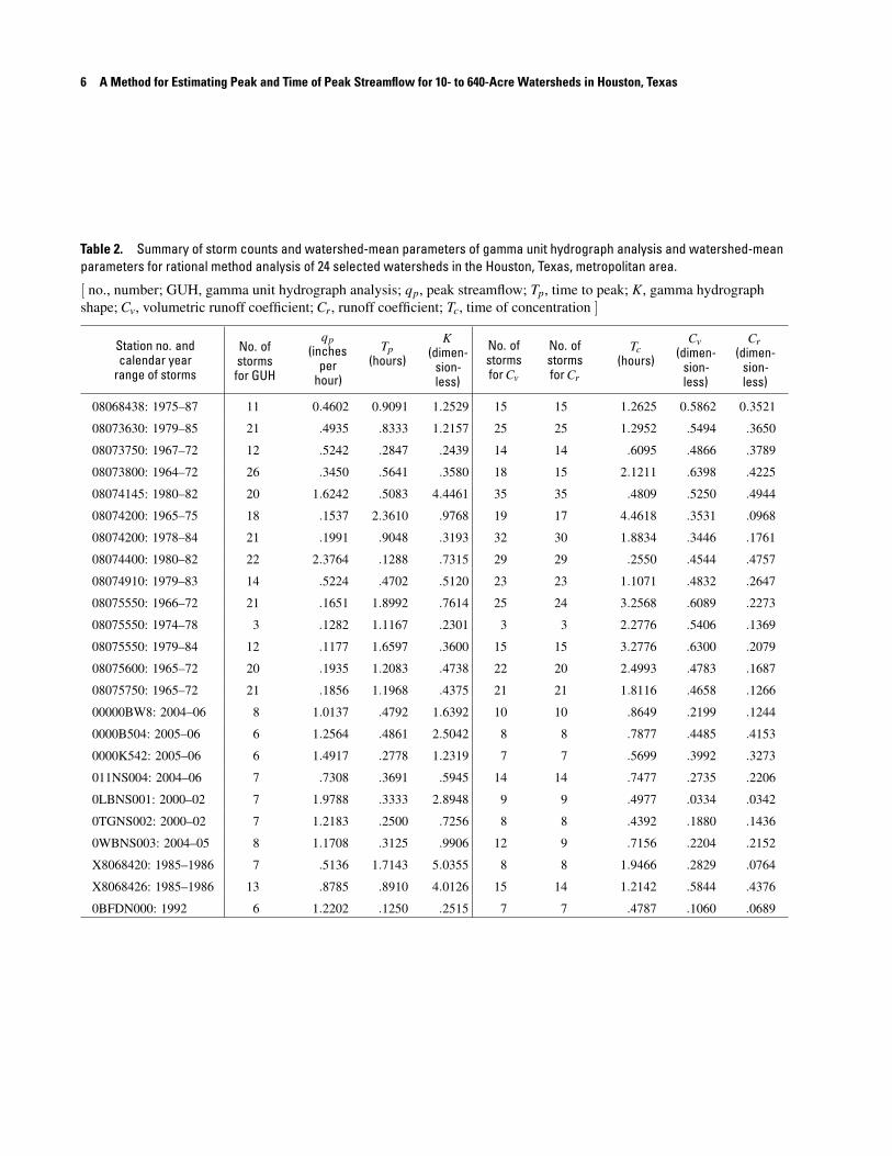
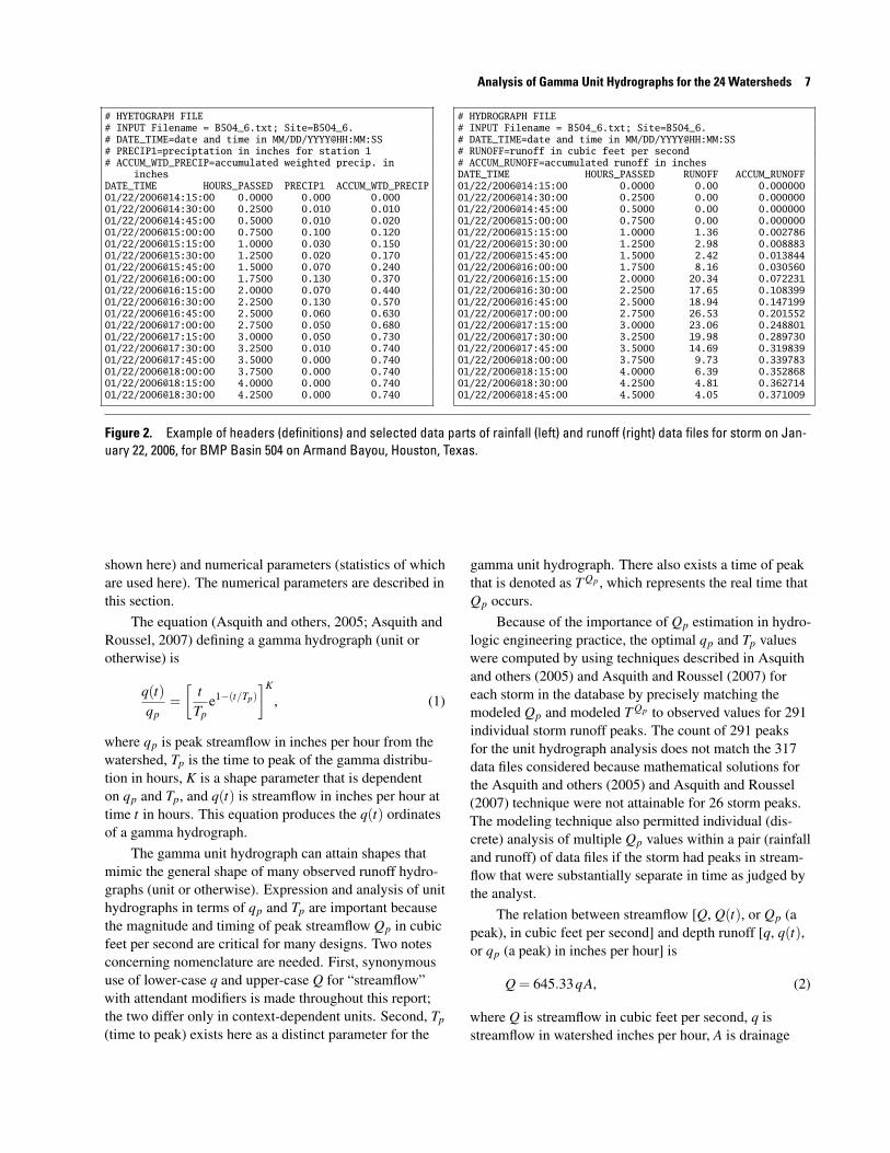
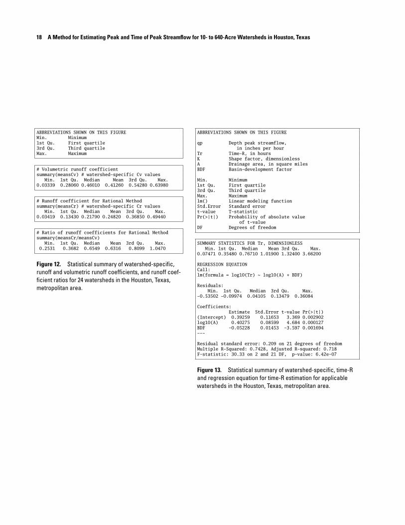
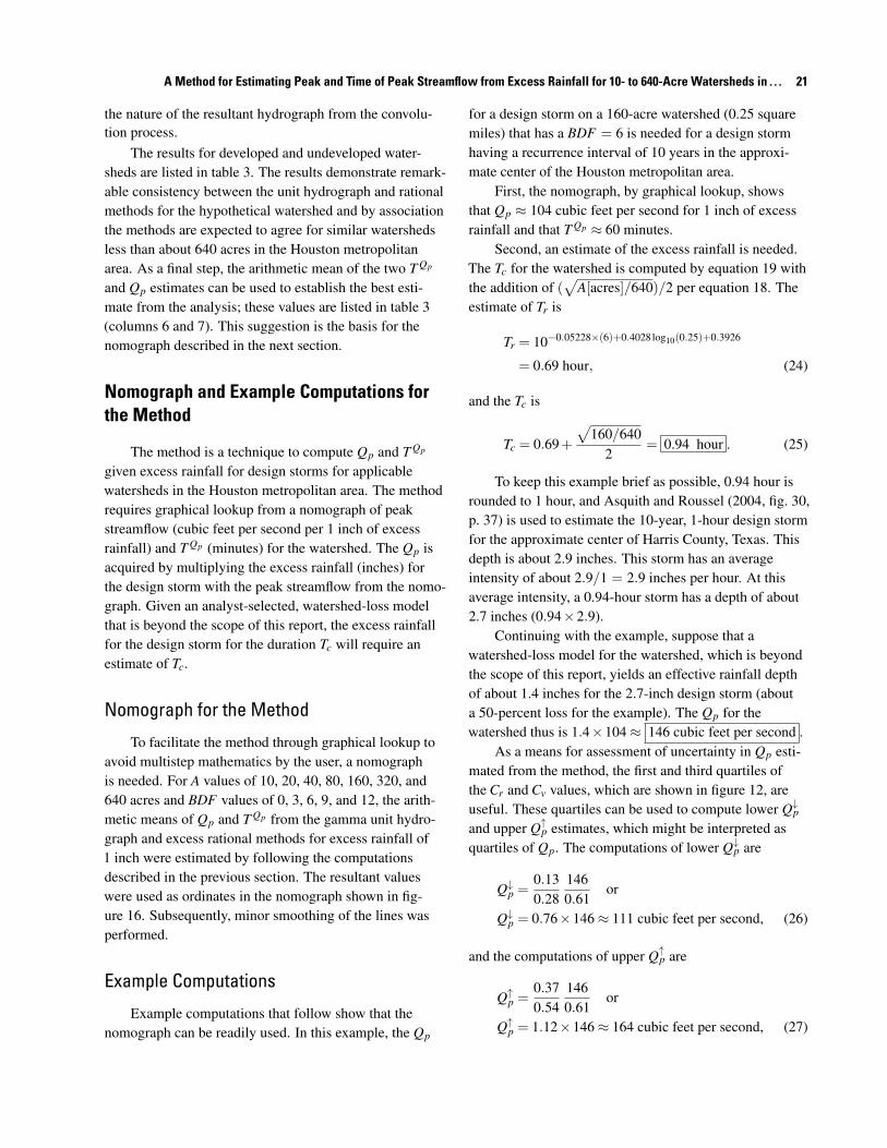