a measurement model of disease damage in paired organs

A Measurement Model of Disease Damage in Paired Organs

Peter Martus

Department of Medical InformaticsBiometry and EpidemiologyFree University Berlin

Summary

Diagnostic test can be used to classify subjects as “diseased” or “undiseased”. If measurements areobtained on a quantitative scale they may serve additionally to quantify the damage caused by thedisease. If a whole bundle of measurements is available but no gold standard exists, the evaluation ofthese measurements may be improved by using latent variables. The subject of this investigation is anapplication of latent variable techniques in the evaluation of diagnostic measurements concerningpaired organs. A method is presented which allows to quantify the association between the true diseasedamage of affected organs. Furthermore, the corresponding association of the error components ofseveral measurements can be quantified. The method is based upon a one factor model of the diagnos-tic measurements. The method supports the investigation of the pathogenetic process of the underlyingdisease and the improvement of diagnostic measurements. It is applied to data from the ErlangenGlaucoma Registry.

Key words: Latent variables; Measurement model; Paired organs; Glaucoma.

Zusammenfassung

Diagnoseverfahren konnen Probanden als „krank“ oder „nicht krank“ klassifizieren. Wenn die Messungenauf einer quantitativen Skala erfolgen, konnen Sie zusatzlich dazu dienen, den Schweregrad der betreffen-den Erkrankung zu quantifizieren. Wenn ein ganzes Bundel von Messungen verfugbar ist, aber kein echter“Goldstandard” existiert, konnen derartige Messverfahren mit Hilfe von Latenten Variablen bewertet wer-den. Thema der hier vorgelegten Arbeit ist die Anwendung der Methodik Latenter Variablen fur die Eva-luation diagnostischer Messungen an paarigen Organen. Es wird ein Ansatz vorgestellt, der es erlaubt, dieAssoziation zwischen den betroffenen Teilorganen zu quantifizieren. Weiterhin kann die entsprechendeAssoziation der Messfehler der einzelnen Messverfahren quantifiziert werden. Die Methode basiert aufder Gultigkeit eines Ein-Faktor-Modells fur die untersuchten Diagnoseverfahren und kann sowohl derUntersuchung der Pathogenese der entsprechenden Erkrankung als auch der Verbesserung der Diagnose-verfahren dienen. Sie wird auf Daten des Erlanger Glaukomregisters angewendet.

1. Introduction

Paired data occur in a natural way in the fields of e.g. ophthalmology, nephrology,and otaryngology. These data have to be treated as stochastically dependent: Inconfirmatory analyses corrections for standard errors, significance tests, and confi-

Biometrical Journal 43 (2001) 8, 927–940

# WILEY-VCH Verlag Berlin GmbH, 13086 Berlin, 2001 0323-3847/01/0812-0927 $ 17.50þ.50/0

dence limits have to be applied. In estimation problems optimal weighing factorsincrease efficiency. These problems are the most obvious ones and have beenrealized for a long time in many fields of medical applications (e.g. Ederer,1973). However, these are not the only interesting topics in this setting: In diag-nostic studies it has to be clarified whether subject or site-related classification isdesired. Furthermore it might be useful to include information contributed by thefellow organ into the classification of the selected organ (Martus, 2000).The understanding of the pathogenesis of a disease affecting paired organs can

be improved if the systemic component of the disease can be distinguished fromthe local, site-related one. One important question concerns the relative impactof site-related processes as compared to subject-related ones. If a gold standardfor the quantification of the disease exists, a simple way of determining thedependency of different sites in the pathogenetic process would be comprised bycorrelation analysis between these sites. If agreement between both sites wouldbe of interest, the method proposed by Bland and Altman (1986) could beapplied.The question becomes more complicated if there is no perfect gold standard

measuring the damage of the disease. In this framework we present a measure-ment model which allows to quantify the systemic component of diseases, whichin our application are the glaucoma eye diseases.Our model is based upon the correlation structure of a bundle of quantitative

diagnostic measurements which all quantify the damage of the visual systemcaused by glaucoma but which are sensitive to different components of the visualpathway. The crucial assumption of our model is the conditional independence ofthe procedures under study.We construct a measurement model using 4 diagnostic procedures, which have

been developed to detect glaucoma and to quantify the progress of this disease.Our model comprises information about the systemic or local nature of the dis-ease. Furthermore, also the relative impact of systemic and local error componentscan be quantified. The assumption of conditional independence has been examinedin a different study (Martus et al. 2000; Martus accepted for publication).In Section 2 we describe the clinical example. In Section 3 we present the basic

one-factor model. In Sections 4 and 6 we present the model for paired organs, inSection 5 we discuss the special case of only two measurements, and in Section 7we give the results of our example. In Section 8 we discuss the assumptions andlimitations of our approach and motivate further research.

2. Clinical Example: Measurement of Glaucomatous Damage

Glaucoma is the name of a group of eye diseases, characterized by typical dam-ages of the optic nerve head, often accompanied by elevated intraocular pressureand followed by typical glaucomatous losses of the visual field. The chronic form

928 P. Martus: Disease Damage in Paired Organs

of the disease is one of the major causes of blindness in the industrialized world(American Academy of Ophthalmology, 1998, p. 9). The established diagnosticcriteria of glaucoma are the measurement of the intraocular pressure, inspection ofthe optic nerve head, and the determination of visual field loss (American Acad-emy of Ophthalmology, 1998, p. 67).In the Erlangen Glaucoma Registry several additional diagnostic procedures

have been examined: Perimetry as implemented in our study reveals differentiallight sensitivity measures at 59 points of the entire visual field. The mean defect(MD) is the arithmetic mean of the 59 differences between individual local sensi-tivities and age adjusted norm values (Flammer, 1985). Two electrophysiologicalprocedures reveal the amplitude of a pattern reversal electroretinogram with a ra-pidly reversing black and white stimulus (ERG, Korth et al., 1989), and the peaklatency of a visually evoked potential in response to a blue on yellow patternpresented in the onset-offset mode (VEP, Korth et al., 1994). Finally, we includethe quantitative component of the optic nerve head inspection, the area of theneuroretinal rim (NRR, Jonas, Fernandez, and Naumann, 1992). This area corre-sponds to the number of nerve fibres which are still intact. We investigate a sam-ple of 237 glaucoma patients from the Erlangen Glaucoma Registry, a clinicalregistry for long-term observation of glaucoma patients and subjects with diseasesuspect, which all have been examined with each of the described procedures. Thegold standard of diagnostic classification was the qualitative inspection of the op-tic nerve head by two experienced ophthalmologists.

3. The one-Factor Model of Diagnostic Measures Quantifying Disease Damage

We assume that for a given disease several quantitative diagnostic measurements Yj,ðj ¼ 1; . . . ; JÞ are available. All these measurements quantify the degree of severityG of the underlying disease but none of them serves as a gold standard. Therefore Ghas to be treated as a latent variable which is assumed to measure the severity of thedisease without error. We are interested in the correlations rj, ðj ¼ 1; . . . ; JÞ betweenthe diagnostic measurements Yj and G. It has been discussed elsewhere (Martuset al., 2000, Martus, accepted for publication) that these correlations serve to quan-tify the validity of the measurements Yj. Given the sample correlations rjk betweenmeasurements j and k ðj; k ¼ 1; . . . ; JÞ the correlations rj can be estimated if themeasurements Yj are independent conditionally on G, the true severity of disease:We start with equations

Yj ¼ bj � G þ xj ðj ¼ 1; . . . ; JÞ : ð1Þ

In these equations xj describes the residual term for measurement j. xj is assumedto be independent from G for j ¼ 1; . . . ; J. If all procedures Yj and the gold stand-ard G are standardized, bj is equal to rj and Var ðxjÞ ¼ 1� b2

j . Conditional inde-pendence of Yj and Yk is equivalent to independence of xj and xk. If this assump-

Biometrical Journal 43 (2001) 8 929

tion is fulfilled we have

rjk ¼ rj � rk : ð2ÞIf at least three diagnostic measurements are available and the assumption of con-ditional independence is fulfilled, the correlations rj ðj ¼ 1; . . . ; JÞ between theunobservable variable G and the observable variables Yj can be determined bysolving the system of equations (2) ðj; k ¼ 1; . . . ; J; j 6¼ kÞ. In the case of threemeasurements the exact solution is

rj ¼ffiffiffiffiffiffiffiffiffiffiffiffiffiffiffirjk � rjl

rkl

rðj; k; l ¼ 1; . . . ; J; j 6¼ k 6¼ l 6¼ jÞ :

If more than three measurements are available, rj has to be estimated according tosome optimality criterion (Bollen, 1989, pp. 104–123, 254; Fahrmeier, Ha-merle and Tutz, 1996, pp. 745–748).Equations (1) can be described equivalently by using path diagrams. In these

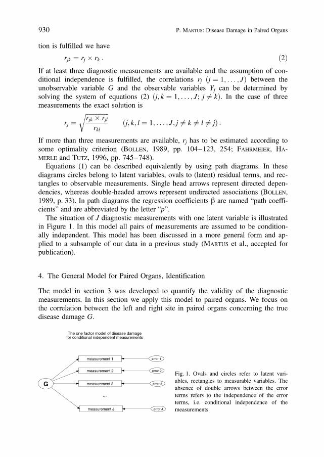
diagrams circles belong to latent variables, ovals to (latent) residual terms, and rec-tangles to observable measurements. Single head arrows represent directed depen-dencies, whereas double-headed arrows represent undirected associations (Bollen,1989, p. 33). In path diagrams the regression coefficients b are named “path coeffi-cients” and are abbreviated by the letter “p”.The situation of J diagnostic measurements with one latent variable is illustrated

in Figure 1. In this model all pairs of measurements are assumed to be condition-ally independent. This model has been discussed in a more general form and ap-plied to a subsample of our data in a previous study (Martus et al., accepted forpublication).

4. The General Model for Paired Organs, Identification

The model in section 3 was developed to quantify the validity of the diagnosticmeasurements. In this section we apply this model to paired organs. We focus onthe correlation between the left and right site in paired organs concerning the truedisease damage G.


G measurement 3

measurement 1

measurement J

error 3

error 2

error 1

error J

measurement 2

The one factor model of disease damagefor conditional independent measurements

...

Fig. 1. Ovals and circles refer to latent vari-ables, rectangles to measurable variables. Theabsence of double arrows between the errorterms refers to the independence of the errorterms, i.e. conditional independence of themeasurements

We assume that J diagnostic measures are obtained from two sites l (left) and r(right) per patient, so that 2*J measurements are available from each subject. Thegeneral model equation is

Yjs ¼ bjs � Gs þ xjs ðj ¼ 1; . . . ; J; s ¼ l; rÞ :

Yjs is measurement j ðj ¼ 1; . . . ; JÞ from site s ðs ¼ l; rÞ; Gs is the latent variableof the true damage of the disease at site s and xjs is the residual term for measure-ment j at site s. The following assumptions will be used in the sequel withj; j0 ¼ 1; . . . ; J; s; s0 ¼ l; r:

1 Yjs and Gs are standardized with expectation zero and variance one;2 E(xjs) ¼ 0;3 xjs and Gs are independent;4 Gl and Gr are identically distributed;5 xjr and xjl are identically distributed;6 (xjr , xj0l) and (xjl , xj0r) are identically (bivariately) distributed;7 xjs and xj0s are independent for j 6¼ j0;8 xjs and xj0s0 are independent for j 6¼ j0, s 6¼s0;9 xjs and Gs0 are independent for s6¼s0.

Assumptions 1–3 are purely conventional, assumptions 4–6 concern the sym-metry between left and right sites. Assumptions 8 and 9 are plausible if assump-tion 7 is fulfilled. This assumption, however, is the crucial one which has to bejustified by several methods (Martus, accepted for publication). The coefficientsbjs are the path coefficients from the one-factor model of site s as described inSection 3. By assumption 1 they are identical to the correlations between Gs andYjs. The above assumptions imply bjl ¼ bjr for j ¼ 1; . . . ; J, i.e. the same one-factor model with identical parameter values is valid for left and right eyes. Thuswe will use the notation “bj” if the symmetry assumption are fulfilled. The covar-iance of two measurements

Yjs ; Yj0s0

which is equal to the correlation of both measures from assumption 1, is given by

bj � bj0 � cov ðGs;Gs0 Þ þ cov ðxj; s; xj0; s0 Þ ð3Þwith

cov ðGs;Gs0 Þ ¼ cor ðGs;Gs0 Þ ;

cov ðxj; s; xj0; s0 Þ ¼ cor ðxj; s; xj0; s0 Þ �ffiffiffiffiffiffiffiffiffiffiffiffiffiffiffiffiffiffiffiffiffiffiffiffiffiffiffiffiffiffiffiffiffiffiffiffiffiffiffið1� b2

j Þ � ð1� b2j0 Þ

q:

If s ¼ s0, clearly cor ðGs;Gs0 Þ ¼ 1. If j ¼ j0 and s 6¼ s0, i.e. the same measurementis correlated between left and right eyes, the above term (3) simplifies tob2

j* cor ðGl;GrÞ þ cov ðxjl; xjrÞ. For j 6¼ j0 and s ¼ s0 from the conditional indepen-

dence of the measurements we obtain cor ðYl; YrÞ ¼ b*j bj0 and if j 6¼ j0 and s 6¼ s0

we get cor ðYl; YrÞ ¼ b*j b*j0 cor ðGs;Gs0 Þ. Formula (3) can be generalized straight-


forwardly if the symmetry assumptions bjl ¼ bjr are violated, in this case bj has toreplaced by bjs and bj0 has to be replaced by bj0s0.Without any symmetry assumptions, the correlation matrix of our model contains

2� J

2

� �¼ J � ð2J � 1Þ

free parameters. From assumptions 4–6 we can reduce this number to only J2

parameters according to the following restrictions for the correlation matrix:– The correlation between two different measures at the same eye does notdepend upon whether it is the left or the right eye.

– The correlation between two different measures at different eyes does not de-pend upon which measurement is obtained from which site. I.e. the correlationof measurement j1 (left eye) with measurement j2 (right eye) is identical to thecorrelation of measurement j1 (right eye) with measurement j2 (left eye).

If these assumptions hold, only J lateral correlations of identical measures,J*ðJ � 1Þ=2 correlations of different measures at the same eye and J*ðJ � 1Þ=2correlations of different measures at different eyes exist so that J2 free correlationsare contained in the model.If additionally assumptions 7–9 hold, we have J path coefficients, J correlations

between left and right eye’s residual terms for identical measurements, and finallythe parameter of interest: the correlation between the true damage at left and righteye. In summary, 2*J þ 1 free parameters are in the model. This model is dis-played in Figure 2.A necessary condition for the model to be identifiable is J*ð2J � 1Þ 2*J þ 1.

This condition is fulfilled if J > 1, but the model is identifiable only for J > 2(see appendix). However, in the case J ¼ 2 the parameter of main interest, i.e.cor ðGl;GrÞ, is identifiable even if the path coefficients are different for left andright eyes. This will be shown in the following section.


Gleft

Gright

ERG_l

MD_l

VEP_l

VEP_r

MD_r

ERG_r

e_VEP_l

e_VEP_r

e_MD_l

e_MD_r

e_ERG_l

e_ERG_r

p2

p4

p2

p3

NRR_l

NRR_r

e_NRR_l

e_NRR_r

p1

p3

p4

p1

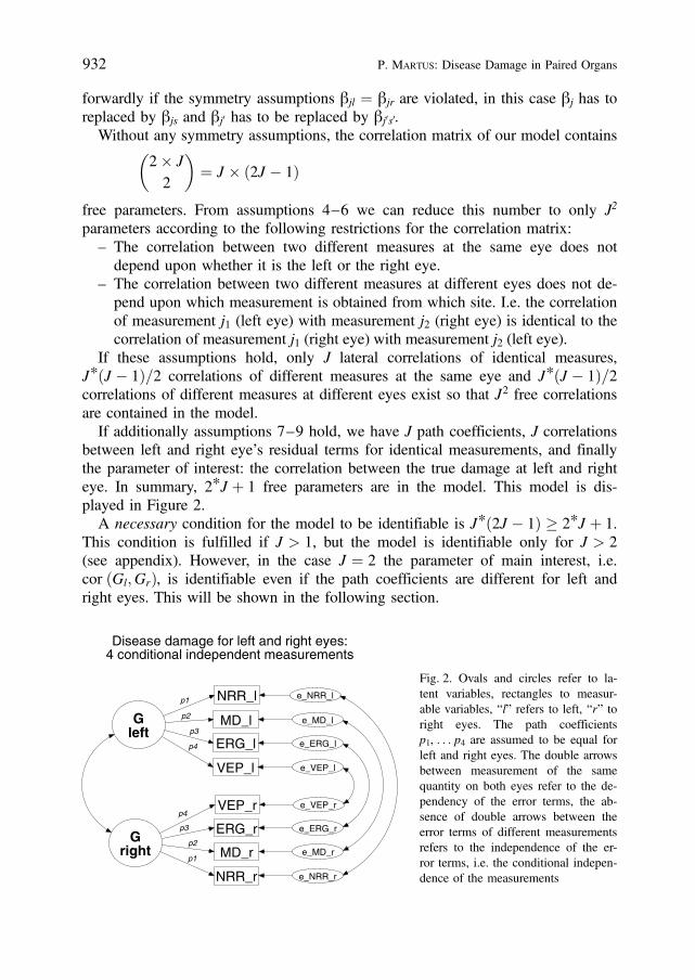
Disease damage for left and right eyes:4 conditional independent measurements

Fig. 2. Ovals and circles refer to la-tent variables, rectangles to measur-able variables, “l” refers to left, “r” toright eyes. The path coefficientsp1, . . . p4 are assumed to be equal forleft and right eyes. The double arrowsbetween measurement of the samequantity on both eyes refer to the de-pendency of the error terms, the ab-sence of double arrows between theerror terms of different measurementsrefers to the independence of the er-ror terms, i.e. the conditional indepen-dence of the measurements

5. A Special Case: Two Conditionally Independent Diagnostic Measurements

In the following we investigate the model displayed in Figure 2 for J ¼ 2 meas-urements. We assume that the measurements are independent conditionally on Gbut we don’t need the assumption of identical path coefficients for left and righteyes. Therefore the model equations are

Y1l ¼ b1l � Gl þ x1l

Y1r ¼ b1r � Gr þ x1r

Y2l ¼ b2l � Gl þ x2l

Y2r ¼ b2r � Gr þ x2r :

From the first law of path analysis (Kenny (1979), p. 28) or directly from equa-tions (3) and the remark on asymmetric coefficients bjl 6¼ bjr we obtain

cor ðY1l; Y1rÞ ¼ b1l � b1r � cor ðGl;GrÞ þ cov ðx1l; x1rÞcor ðY2l; Y2rÞ ¼ b2l � b2r � cor ðGl;GrÞ þ cov ðx2l; x2rÞcor ðY1l; Y2lÞ ¼ b1l � b2l

cor ðY1r; Y2rÞ ¼ b1r � b2r

cor ðY1l; Y2rÞ ¼ b1l � b2r � cor ðGl;GrÞcor ðY1r; Y2lÞ ¼ b1r � b2l � cor ðGl;GrÞ :

In this system of equations neither bjs nor cov (xjl, xjr) are identified even if bjl ¼ bjr

holds for j ¼ 1; 2. Nevertheless, from the last four equations we have

cor ðGl;GrÞ ¼

ffiffiffiffiffiffiffiffiffiffiffiffiffiffiffiffiffiffiffiffiffiffiffiffiffiffiffiffiffiffiffiffiffiffiffiffiffiffiffiffiffiffiffiffiffiffiffiffiffiffiffiffiffiffiffiffiffiffiffifficor ðY1l;Y2rÞ � cor ðY1r; Y2lÞcor ðY1l;Y2lÞ � cor ðY1r; Y2rÞ

� �sð4Þ

and therefore the parameter of main interest, cor ðGl;GrÞ, indeed is the only iden-tifiable parameter.

6. Estimation and Model fit

Estimation of parameters and standard errors is performed using the methods de-veloped for structural equation models. These methods have been described inseveral textbooks and will not be presented in detail here (Bollen, 1989; Fahr-meier et al., 1996, chap. 11). An overview focussed on medical application isgiven in Bentler and Stein (1992).From the ð2*J þ 1Þ-vector q of path coefficients and lateral correlations of the

latent variable G and the residual terms xjs, the predicted correlation matrix can bederived according to formula (3). Assuming multivariate normally distributed vari-


ables maximum likelihood estimation is achieved by minimizing

FðS;SðqÞÞ ¼ ln jSðqÞj þ tr ½SS�1ðqÞ� � ln jSj � p ð5Þwith observed covariance matrix S, predicted covariance matrix S(q) according to(3), and p being the number of parameters in the model (Bollen, 1989, p. 33). Inthe case of a one-factor model for paired organs with J measurements independentconditionally on G, p ¼ 2*J þ 1.If the assumption of normality is fulfilled, standard errors can be derived from

the covariance matrix of qq. In our application we used the software AMOS(Arbuckle, 1997) in which standard errors according to the bootstrap method(Efron, 1979) are available.There are different strategies of examining the goodness of fit in our model.

Assuming normally distributed data and the model to be true, ðN � 1Þ* FðS;SðqÞÞis equal to �2* log ðLÞ, L being the likelihood ratio of the model corresponding toq and the saturated model with S ¼ S. It is distributed according to a chi-squaredistribution with ½J*ð2J � 1Þ � ð2J þ 1Þ� degrees of freedom (Fahrmeier et al.,1996, p. 759).Furthermore, the fit of the model can be examined by the use of modification

indices. These indices quantify the improvement of the fit of the model after inclu-sion of new parameters qp (or more generally after cancelation of fixed values forparameters in the model) or cancelation of equality constraints between parametersqg in the model. The indices can be determined by using first and second deriva-tives of F and the information matrix E of the restricted model (Fahrmeier et al.,1996, pp. 761–763). Thus, they avoid the fit of a new model for every new param-eter. They are approximately chi-square distributed with 1 DF, if the restrictedmodel is true.If more than three measures are available, it is possible to estimate the param-

eters in all submodels with at least three variables. As it has been shown insection 5, the main parameter of interest, the correlation between Gl and Gr, canbe determined in models containing only two diagnostic measurements. The scat-ter of the parameter estimates gives some insight in how well the model fits thedata.

7. Clinical Example: Results

All analyses were performed using the software AMOS (Arbuckle, 1997). Insubmodels with only two measurements, the correlation between Gl and Gr wasdetermined directly from the sample correlations according to formula (4) given inSection 5.In Table 1 the sample correlations are given. The subsequent analyses are based

on these correlations. The symmetry assumptions stated in section 4 are fulfilledfor NRR, MD and ERG. They are, to a certain degree, violated for VEP.


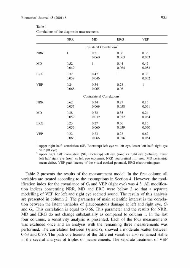
Table 2 presents the results of the measurement model. In the first column allvariables are treated according to the assumptions in Section 4. However, the mod-ification index for the covariance of Gl and VEP (right eye) was 4.3. All modifica-tion indices concerning NRR, MD and ERG were below 2 so that a separatemodelling of VEP for left and right eye seemed sound. The results of this analysisare presented in column 2. The parameter of main scientific interest is the correla-tion between the latent variables of glaucomatous damage at left and right eye, Gl

and Gr. This correlation is equal to 0.66. This parameter and the results for NRR,MD and ERG do not change substantially as compared to column 1. In the lastfour columns, a sensitivity analysis is presented. Each of the four measurementswas excluded once and an analysis with the remaining three measurements wasperformed. The correlation between Gl and Gr showed a moderate scatter between0.63 and 0.70. The path coefficients of the different variables also remained stablein the several analyses of triples of measurements. The separate treatment of VEP


Table 1

Correlations of the diagnostic measurements

NRR MD ERG VEP

Ipsilateral Correlations1

NRR 1 0.510.060

0.360.063

0.360.053

MD 0.520.049

1 0.440.064

0.470.053

ERG 0.320.059

0.470.046

1 0.330.052

VEP 0.240.068

0.340.065

0.280.061

1

Contralateral Correlations2

NRR 0.620.057

0.340.069

0.270.058

0.160.061

MD 0.380.059

0.720.039

0.350.052

0.240.064

ERG 0.230.056

0.270.060

0.660.039

0.160.060

VEP 0.220.063

0.230.066

0.220.056

0.620.054

1 upper right half: correlation (SE, Bootstrap) left eye vs left eye, lower left half: right eyevs right eye;

2 upper right half: correlation (SE, Bootstrap) left eye (row) vs right eye (column), lowerleft half right eye (row) vs left eye (column); NRR neuroretinal rim area, MD perimetricmean defect, VEP peak latency of the visual evoked potential, ERG electroretinogram.

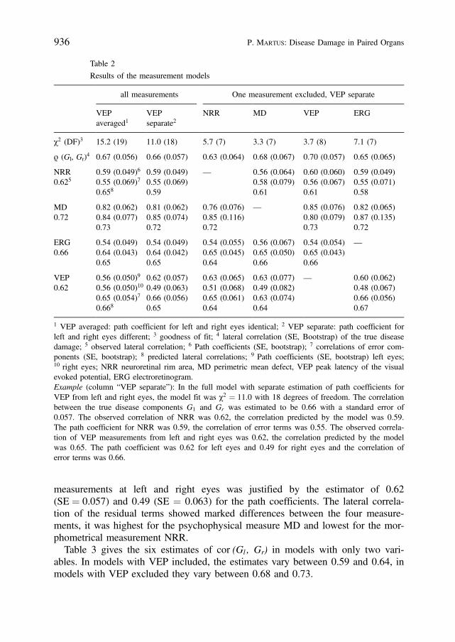
measurements at left and right eyes was justified by the estimator of 0.62(SE ¼ 0.057) and 0.49 (SE ¼ 0.063) for the path coefficients. The lateral correla-tion of the residual terms showed marked differences between the four measure-ments, it was highest for the psychophysical measure MD and lowest for the mor-phometrical measurement NRR.Table 3 gives the six estimates of cor (Gl , Gr) in models with only two vari-

ables. In models with VEP included, the estimates vary between 0.59 and 0.64, inmodels with VEP excluded they vary between 0.68 and 0.73.


Table 2

Results of the measurement models

all measurements One measurement excluded, VEP separate

VEPaveraged1

VEPseparate2

NRR MD VEP ERG

c2 (DF)3 15.2 (19) 11.0 (18) 5.7 (7) 3.3 (7) 3.7 (8) 7.1 (7)

r (Gl, Gr)4 0.67 (0.056) 0.66 (0.057) 0.63 (0.064) 0.68 (0.067) 0.70 (0.057) 0.65 (0.065)

NRR0.625

0.59 (0.049)6

0.55 (0.069)7

0.658

0.59 (0.049)0.55 (0.069)0.59

— 0.56 (0.064)0.58 (0.079)0.61

0.60 (0.060)0.56 (0.067)0.61

0.59 (0.049)0.55 (0.071)0.58

MD0.72

0.82 (0.062)0.84 (0.077)0.73

0.81 (0.062)0.85 (0.074)0.72

0.76 (0.076)0.85 (0.116)0.72

— 0.85 (0.076)0.80 (0.079)0.73

0.82 (0.065)0.87 (0.135)0.72

ERG0.66

0.54 (0.049)0.64 (0.043)0.65

0.54 (0.049)0.64 (0.042)0.65

0.54 (0.055)0.65 (0.045)0.64

0.56 (0.067)0.65 (0.050)0.66

0.54 (0.054)0.65 (0.043)0.66

—

VEP0.62

0.56 (0.050)9

0.56 (0.050)10

0.65 (0.054)7

0.668

0.62 (0.057)0.49 (0.063)0.66 (0.056)0.65

0.63 (0.065)0.51 (0.068)0.65 (0.061)0.64

0.63 (0.077)0.49 (0.082)0.63 (0.074)0.64

— 0.60 (0.062)0.48 (0.067)0.66 (0.056)0.67

1 VEP averaged: path coefficient for left and right eyes identical; 2 VEP separate: path coefficient forleft and right eyes different; 3 goodness of fit; 4 lateral correlation (SE, Bootstrap) of the true diseasedamage; 5 observed lateral correlation; 6 Path coefficients (SE, bootstrap); 7 correlations of error com-ponents (SE, bootstrap); 8 predicted lateral correlations; 9 Path coefficients (SE, bootstrap) left eyes;10 right eyes; NRR neuroretinal rim area, MD perimetric mean defect, VEP peak latency of the visualevoked potential, ERG electroretinogram.Example (column “VEP separate”): In the full model with separate estimation of path coefficients forVEP from left and right eyes, the model fit was c2 ¼ 11.0 with 18 degrees of freedom. The correlationbetween the true disease components G1 and Gr was estimated to be 0.66 with a standard error of0.057. The observed correlation of NRR was 0.62, the correlation predicted by the model was 0.59.The path coefficient for NRR was 0.59, the correlation of error terms was 0.55. The observed correla-tion of VEP measurements from left and right eyes was 0.62, the correlation predicted by the modelwas 0.65. The path coefficient was 0.62 for left eyes and 0.49 for right eyes and the correlation oferror terms was 0.66.

8. Discussion

There is a large literature on the topic of quantifying agreement between differentmeasurement devices (e.g. Fleiss, 1986; Bland and Altman, 1995; Shoukri,1998). If the measurements are defined on identical scales the use of correlationanalyses has been criticized in a series of well known papers by Altman andBland (Altman and Bland, 1983; Bland and Altman, 1986; Bland and Alt-man, 1995). However, in the case of measurements obtained on entirely differentscales, methods related to correlation analysis seem to be acceptable (Chinn,1990).The models used in the preceding sections are measurement models which be-

long to the family of structural equation models, also known as LISREL typemodels (Bentler and Stein, 1992; Bollen, 1989). In these models, observablevariables are used as indicators for unmeasurable, latent variables. The generalstructural equation model consists of two parts: A path model of the latent vari-ables and a measurement model connecting manifest and latent variables. The pathmodel contains directed causal and undirected correlational relationships. Basis ofthe analyses is the correlation or covariance matrix of the manifest variables. In ameasurement model no directed relationship is assumed for the latent variables.In our analysis a measurement model without directed relationships between

latent variables but with correlated residual terms was used. The interpretation ofthe residual term in the model requires a more detailed discussion. First, it con-tains the intrinsic measurement error which theoretically could be reduced to aninfinitely small degree by sufficient repetition or improvement of the measurementdevice. This component, which could be devided further in an observer-relatedand a technical component therefore reflects the quality of implementation of themeasurement. Second, the residual component contains the short term fluctuationsof the true value. From the practical point of view this component could be elimi-nated by repeated measurements in the same way as the measurement error. Third,the residual term contains the longterm fluctuation of the true quantity measuredand this fluctuation of course could be quantified and eliminated by repeated meas-urements in a longterm setting. If the model presented in this investigation would


Table 3

Estimation of cor (Gl,Gr) from all possible pairs of measurements

measurement 1 NRR NRR MD NRR MD ERG

measurement 2 MD ERG ERG VEP VEP VEP

estimate cor (Gl, Gr) 0.70 0.73 0.68 0.64 0.59 0.62

NRR neuroretinal rim area, MD perimetric mean defect, VEP peak latency of the visualevoked potential, ERG electroretinogram.

be combined with a study of longterm- and shortterm reproducibility, the residualterm principally could be splitted in the components just described.On the other hand, the residual term additionally contains the true biological

variability of the underlying trait. This biological variability is not affected byoptimization or repetition of the measurement procedure. To give an example, thearea of the neuroretinal rim could be determined theoretically with a perfect meas-urement device. However, from this it is not clear that the correlation of the truerim area with the true glaucomatous damage would be equal to 1, as e.g. the truerim area is also affected by the biological variability between subjects. In theanalysis of laboratory measurements this reproducible component of the residualterm is called a “random matrix effect”. This term refers to the material or med-ium in which the substance to be measured is embedded or dissolved, e.g. bloodserum (Dunn and Roberts, 1999). In our setting, the variability of this specificcomponent of the residual term quantifies the validity of the measurement ratio-nale. Especially in a complex and only partly understood disease like glaucomathese random matrix effects are likely to be present in any diagnostic measure-ment. Therefore, in no instance the simple repetition of the same measurementcould provide independent residual terms.In our analysis the total residual terms showed correlations between 0.55 (NRR)

and 0.85 (MD). It seems plausible that the high correlation for the psychophysicalmeasurement MD is due to the concentration of the patient, the correlation of theerror term was estimated to be 0.84, therefore about 70% of the whole residualvariance being subject-related. An improvement of this measurement device there-fore might be achieved by reducing the measurement error due to the complianceof the patient. In contrast, the residual terms of NRR only shows a small lateraldependency with about 30% of the whole residual variance being subject-related.The sensitivity analysis of our model revealed a somehow inconsistent pattern

of estimators for the correlations of disease damage at left and right site, depend-ing on whether the measurement VEP was included in the analysis or not: In themodels excluding VEP, cor (Gl, Gr) was estimated between 0.68 and 0.73, in themodels including VEP estimators took values between 0.59 and 0.66. It is not thepurpose of this study to discuss in detail the ophthalmological implications of thisobservation. However, as VEP was the only variable which showed severe viola-tions of symmetry assumptions for left and right eyes the range of 0.68 to 0.73seems to be realistic for a point estimator of cor (Gl, Gr).An explanation for the observed asymmetry in the visual evoked potential

(VEP) might be that this measurement is always performed first at the right eye. Itseems plausible, that during the second measurement the proband gets more usedto the device. Thus left-eye measurements may be influenced by smaller errorterms, which results in a higher validity, i.e. a greater path coefficient, of themeasurements at left eyes. A similar result was found for the discrimination be-tween patients and controls (Martus, 2000). However, the same argument appliesto the electroretinogram (ERG) where no asymmetries have been found.


Acknowledgement

I thank G. O. H. Naumann, J. B. Jonas, and M. Korth for permission of use ofdata from the Erlangen Glaucoma Registry.

Appendix: Identification of the General Model for More than 2 Measurements

We assume that assumptions 1–8 from Section 4 are fulfilled. We will show thatfor any set of three measurements the corresponding submodel is identifiable.From equations

Y1l ¼ b1 � Gl þ x1l



we obtain exact solutions for the coefficients bj ðj ¼ 1; 2; 3Þ analogous to Kenny(1979), p. 41. With known path coefficients b1, b2 we obtain from e.g.

cor ðY1l; Y2rÞ ¼ b1 � b2 � cor ðGl;GrÞa solution for cor (Gl, Gr), and finally from the equations of the form

cor ðYij; YjrÞ ¼ bj � bj � cor ðGl;GrÞ þ cov ðxjl; xjrÞ

we obtain solutions for cov (xjl, xjr) ðj ¼ 1; 2; 3Þ.If there are more than three measurements all parameters with the exception of

cov (xjl, xjr) are even overidentified.

References

Arbuckle J. L., 1997: Amos Users’ Guide Version 3.6. SmallWaters Corporation, Chicago.Altman, D. G. and Bland, J. M., 1983: Measurement in medicine: the analysis of method comparison

studies. Statistician 32, 307–17.American Academy of Ophthalmology, 1998: Basic and Clinical Science Course 1998–1999, Sec-

tion 10. Glaucoma. AAO, San Francisco.Bentler, P. M. and Stein, J. A., 1992: Structural equation models in medical research. Statistical

Methods in Medical Research 1, 159–181.Bland, J. M. and Altman, D. G., 1986: Statistical methods for assessing agreement between two

methods of clinical measurement. Lancet i, 307–10.Bland, J. M. and Altman, D. G., 1995: Comparing two methods of clinical measurement: A personal

history. International Journal of Epidemiology 24 (Suppl. 1), S7–S14.Bollen, K. A., 1989: Structural Equations with latent variables. Wiley, New York.Chinn, S., 1990: The assessment of methods of measurement. Statistics in Medicine 9, 351–362.Dunn, G. and Roberts, C., 1999: Modelling method comparison data. Statistical Methods in Medical

Research 8: 161–179.Ederer, F., 1973: Shall we count numbers of eyes or numbers of subjects? Archives of Ophthalmology

89, 1–2.


Efron, B., 1979: Bootstrap methods: Another look at the jackknife. Annals of Statistics 7, 1–26.Fahrmeier, L., Hamerle, A., and Tutz, G. (eds.), 1996: Multivariate statistische Verfahren (2. ed.). de

Gruyter, Berlin.Flammer, J., 1985: The concept of visual field indices. Graefe’s Archive of Clinical and Experimental

Ophthalmolology 224, 389–392.Fleiss, J. L., 1986: Design and Analysis of Clinical Experiments (reprint 1999). Wiley, New York.Jonas, J. B., Fernandez, M. C., and Naumann, G. O. H., 1992: Glaucomatous parapapillary chorior-

etinal atrophy: Occurence and correlations. Arch Ophthalmol. 110, 214–22.Kenny, D. A., 1979: Correlation and causality. Wiley, New York.Korth, M., Horn, F., Storck, B., and Jonas, J. B., ‘The pattern-evoked electroretinogram (PERG):

Age-related alterations and changes in glaucoma’, 1989: Graefe’s Archive of Clinical and Experi-mental Ophthalmolology 227, 123–130.

Korth, M., Nguyen, N. X., Junemann, A., MARTUS, P. and Jonas, J. B., 1994: ‘VEP test of theblue-sensitive pathway in glaucoma’, Investigative Ophthalmolology and Visual Science 35, 2599–2610.

Martus, P., Junemann, A., Wisse, M., Budde, W. M., Horn, F., Korth, M., and Jonas, J. B.: Amultivariate approach for quantification of morphologic and functional damage in glaucoma, In-vestigative Ophthalmolology and Visual Science 2000 41, 1099–1110.

Martus, P.: Statistical Methods for diagnostic models concerning paired organs. Statistics in Medicine2000 19, 525–540.

Martus P.: A measurement model for disease severity in absence of a gold standard. Methods ofinformation in medicine (accepted for publication).

Shoukri, M. M., 1998: Agreement, Measurement of. In: Armitage, P. and Colton, T. (eds) Encyclope-dia of Biostatistics Vol.1, 103–117. Wiley, New York.

Dr. P. Martus Received, November 1999Hindenburgdamm 3 Revised, May 2001Institut fur Medizinische Informatik Accepted, May 2001Biometrie und EpidemiologieD-12200 BerlinGermany


a measurement model of disease damage in paired organs

Documents