a mathematical optimization approach for resource ... · a mathematical optimization approach for...

A Mathematical Optimization Approach for Resource Allocation in Large Scale Data Centers Cipriano Santos, Xiaoyun Zhu, Harlan Crowder Intelligent Enterprise Technologies Laboratory HP Laboratories Palo Alto HPL-2002-64 (R.1) December 12th , 2002* E-mail: {cipriano_santos, xiaoyun_zhu, harlan_crowder}@hp.com mathematical programming, Internet data center, resource allocation, scalability

In this paper, we address the resource allocation problem (RAP) for large scale data centers using mathematical optimization techniques. Given a physical topology of resources in a large data center, and an application with certain architecture and requirements, we want to determine which resources in the physical topology should be assigned to the application architecture such that application requirements and bandwidth constraints in the network are satisfied, while communication delay between assigned servers is minimized. We have decomposed this complex combinatorial optimization problem into a series of tractable mathematical optimization models that can be easily solved using commercially available mathematical programming solvers. Preliminary tests of this approach demonstrated consis tently that optimal or “good” solutions for problems from small to large scales can be found in seconds, which proves its better scalability compared to a Layered Partitioning and Pruning (LPP) algorithm in previous work. In addition, this Mathematical Programming approach can be extended to more general problems using the same solvers, that is, extensions of the original problem do not require the development of new algorithms.

* Internal Accession Date Only Approved for External Publication Presented at the Informs Annual Meeting, 17-20 November 2002, San Jose, CA Copyright Hewlett-Packard Company 2002

- 1 -

A M athem atical Optim ization Approach for Resource Allocation in Large Scale Data Centers

Cipriano Santos Xiaoyun Zhu Harlan Crowder

Hewlett Packard Labs Palo Alto, CA 94304

{cipriano_santos, xiaoyun_zhu, harlan_crowder}@hp.com

Abstract In this paper, we address the resource allocation problem (RAP) for large scale data centers using mathematical optimization techniques. Given a physical topology of resources in a large data center, and an application with certain architecture and requirements, we want to determine which resources in the physical topology should be assigned to the application architecture such that application requirements and bandwidth constraints in the network are satisfied, while communication delay between assigned servers is minimized. We have decomposed this complex combinatorial optimization problem into a series of tractable mathematical optimization models that can be easily solved using commercially available mathematical programming solvers. Preliminary tests of this approach demonstrated consistently that optimal or “good” solutions for problems from small to large scales can be found in seconds, which proves its better scalability compared to a Layered Partitioning and Pruning (LPP) algorithm in previous work. In addition, this Mathematical Programming1 approach can be extended to more general problems using the same solvers, that is, extensions of the original problem do not require the development of new algorithms. Keywords: Internet data center, resource allocation, mathematical programming, scalability 1 Introduction Internet Data Centers (IDCs) aim to provide highly available, scalable, flexible, and secure information technology (IT) infrastructure and services to both Applications Service Providers (ASPs) --- companies that offer individuals or businesses Internet-based access to applications and related services --- and enterprises with internal IT requirements. The recent shakeout of high-profile ASP and IDC providers – including several spectacular bankruptcies – has shifted the focus and business model of the surviving companies from “growth and market share at any cost” to more conservative, old fashion objectives such as profitability management and optimizing the effectiveness and efficiency of existing resources. IDC providers can be classified into two categories. Some are co-location service providers that lease secure IDC space and network connectivity to corporations or third party ASPs. Others are referred to as Managed Service Providers (MSPs), who own the servers in the IDC and provide value-added services including security, performance monitoring, content distribution, and capacity planning. In addition, many IDCs are themselves ASPs who manage not only the infrastructure but also the applications. As we move towards the world of utility computing, MSPs are of particular interest to us because they offer the potential for further sharing the infrastructure among different customers and applications, thus increasing the resource utilization in the data centers. Recently, IDCs have grown significantly in both size and complexity. Some IDCs today consist of tens of thousands of servers with high-speed network connections for both inter- and intra-IDC communications. Managing both infrastructure and applications in such large and complex environments raises many challenges since IDC operating costs can escalate very quickly, damaging the profitability of these businesses. The key to effective management of these large data complexes is to continually evaluate and

1 In this paper, we use the terms mathematical programming and mathematical optimization indistinctly.

- 2 -

refine business models and processes, and to employ decision support and automation tools for assessing performance and making good operational and strategic decisions. The business model we want to address in this paper is the sharing of resources among applications in an IDC. A key driver for this model is the need for an IDC to manage a suite of complex applications with diverse requirements and dynamic characteristics based on service-level agreements. On one hand, some Web applications experience highly bursty traffic whose workload intensity varies dramatically during different time of day, or day of week. Over-provisioning, a common practice today, turns out to be a highly inefficient way for capacity planning. If resources are allocated based on maximum usage, there will be periods when the system activity level is extremely low and the resources are very poorly utilized. In addition, special promotions come and go with peak demands much higher than the regular usage, which makes over-provisioning even infeasible to implement. On the other hand, there may be fairly predictable batch processing jobs that can utilize resources when they are not needed for other applications. Therefore, where applicable, an application should not be bound to a particular piece or set of hardware devices, but rather the application-resource assignment should be made dynamically by IDC management processes. This is often referred to as “capacity on demand.”[5] This business model is desirable because it allows IDC resources to be leveraged across many applications, with significant economies of scale. But the downside is a significant increase in the complexity of IDC operations that requires new levels of sophistication in both workload demand and resource capacity management. In this paper, we address the Resource Allocation Problem (RAP) that is inherent in any IDC that shares resources among applications. In simple terms, the RAP is:

Given a physical network topology of nodes consisting of switches and servers in an IDC, and application requirements architecture, we need to determine which servers in the physical topology should be assigned to the application architecture. Any such assignments much obey two rules: (1) the application requirements and bandwidth constraints of the nodes in the physical topology must be satisfied, and (2) the average communication delay between the assigned servers is minimized.

The RAP problem was originally formulated by Zhu and Singhal, and a layered partitioning and pruning (LPP) method was proposed to solve this problem [7]. While their method captures the essential elements of the problem, their computational solution method is not scalable to contemporary-sized IDC architecture. The mathematical optimization approach in this paper is based on the core ideas of the LPP algorithm, but the procedural approach of LPP has been translated into a declarative approach, a sequence of mathematical optimization models that can be solved efficiently by commercially available solvers such as CPLEX2 and MINOS3. The RAP problem is present either when applications are initially deployed in an IDC, or when changes in workload intensity require that resources be added to or removed from an application. The mathematical programming models presented in this paper deal with the initial allocation process in particular. However, the models are easily extensible to handle dynamic incremental resource allocations to an existing application. The IBM “Oceano” project also focuses on the concept of “capacity on demand” and addresses the problem of dynamic resource allocation. [1] However, there has not been any published work on this subject using analytical techniques. In the meantime, the TAO (Transactions, Analysis, and Optimization) project of HP Labs is investigating the issues in integrating workload characterization and resource capacity planning using a combination of analytical tools and an experimental test bed. The work presented in this paper is essentially complementary to the research conducted in the TAO project. For more details about the TAO project see Garg et al [3].

2 CPLEX is an ILOG software product for solving Linear and Mixed Integer programming problems. For more information visit the following website, www.ilog.com. 3 MINOS is software developed by Professors Walter Murray and Michael Saunders from Stanford University, and Professor Phillip Gill from UC San Diego for solving Non-linear programming problems. For more information visit the following site, www.sbsi-sol-optimize.com.

- 3 -

2 RAP Definition and an Example For a given physical network topology of an IDC, a given application with a tiered architecture, and resource requirements for the application, the problem is to allocate servers in the topology into the tiered architecture such that the application resource requirements are satisfied and the average communication delay between servers (also known as latency) is minimized. The following example illustrates an instance of RAP. 2.1 Network Topology An IDC network topology is illustrated in Figure 1. The topology is characterized by:

• The layout of the network topology is a hierarchical tree. The root of the tree is a mesh switch, an abstraction of a tightly connected group of switches acting as a single device.

• Below the root are two edge switches, labeled Edge 1 and Edge 2. • Below the edge switches are four rack switches: Rack 1 through Rack 4. • At the bottom of the tree are 12 servers, Server 1 through Server 12. • Each server has 3 attributes: number of CPUs, CPU speed, and memory size. Server attributes are

summarized in Table 1. For example, Server 1 has 8 CPUs of 400 MHz each and 4 GB of random access memory. (Note that other instances of RAP may require more server attributes.)

• Each server, rack switch, and edge switch has an incoming and outgoing bandwidth capacity, measured in Gbps. These capacities are summarized in Table 2. For example, both the incoming and outgoing bandwidth capacity of Server 1 is 2.0 Gbps.

Edge 1 Edge 2

Rack 1 Rack 2 Rack 3 Rack 4

Server 10 Server 12

Server 11

Server 7 Server 9

Server 8

Server 4 Server 6

Server 5

Server 1 Server 3

Server 2

Mesh Switch

Edge Switches

Rack Switches

Servers

Figure 1. Example of network topology

1 2 3 4 5 6 7 8 9 10 11 12

CPU Speed (MHz) 400 400 400 500 500 500 400 500 500 400 400 500Number of CPUs 8 8 8 10 10 10 8 10 10 8 8 10RAM (GB) 4.0 4.0 4.0 16.0 16.0 16.0 4.0 16.0 16.0 4.0 4.0 16.0

Servers

Table 1. Example of server attributes

1 2 1 2 3 4 1 2 3 4 5 6 7 8 9 10 11 12

Input (Gbps) 4.0 4.0 4.0 4.0 4.0 4.0 2.0 2.0 2.0 2.0 2.0 2.0 2.0 2.0 2.0 2.0 2.0 2.0Output (Gbps) 4.0 4.0 4.0 4.0 4.0 4.0 2.0 2.0 0.5 2.0 2.0 0.4 2.0 2.0 0.5 2.0 2.0 2.0

Edge S. Rack Switchs Servers

Table 2. Example of server and switch bandwidth

- 4 -

2.2 Application Architecture The application architecture for the example is illustrated in Figure 2 and is characterized by:

• A three-tier architecture consisting of Web, application and database servers. We have labeled these tiers L1, L2 and L3.

• Tiers L1 and L2 require two servers each. L3 requires one server. • The servers in each tier have minimum and maximum values for the required attributes. These

requirements are summarized in Table 3. For example, the minimum and maximum CPU speed for any server in tier L1 is 200MHz and 500MHz, respectively.

• At the top of Figure 2 are notations that indicate the maximum amount of data traffic, measured in Gbps, going from each server in a tier to each server in a consecutive tier. In this example, the maximum amount of traffic from each server in tier L1 to each server in tier L2 is 0.2Gbps.

DB

Apps

Apps W eb

W eb

0.15Gbps

0.15G bps

0.2G bps

0.2G bps

0.2G bps

0.2G bps

L3: DatabaseServers

L2: ApplicationServers

L1: W ebServers

Figure 2. Example of tiered application architecture

min max min max min maxCPU Speed 200 500 400 600 500 INFCPU Number 4 10 8 16 10 INFRAM 4.0 12.0 4.0 16.0 10.0 INF

Note: INF = no bound specified

TiersL1 L2 L3

Table 3. Example of application requirements on servers

Our problem is to identify which servers in the physical topology should be allocated to each tier in the application such that latency is minimized while bandwidth constraints and Min/Max server attribute requirements are satisfied. 3 Mathematical Formulation of RAP The mathematical formulation is based on the following assumptions.

1. The physical topology is a hierarchical tree.4 4 We define a hierarchical tree as the tree where the set of nodes can be partitioned into levels. Level zero is the root of the tree, level 1 is the set of children of level 0, level 2 is the union of the sets of children of each node in level 1, etc.

- 5 -

2. The application has a tiered architecture. 3. Servers at the same tier have the same functionality. Consequently, they have the same attribute

requirements. 4. The amount of traffic generated by different servers in the same tier is similar. And the amount of

traffic coming into each tier is evenly distributed among all the servers in the tier. 5. No traffic goes between servers in the same tier.

The reasoning behind these assumptions was described in [7]. When it is necessary to consider applications with more general architecture or traffic characteristics, the mathematical models presented below can be easily extended to deal with these variations. The following notation is used to describe the mathematical formulation of RAP. Sets and their indices

Ll ∈ : Set of tiers or layers, where L represents the number of tiers. [Alternative index i]

Ss ∈ : Set of servers. S represents the number of servers. [Alternative index j]

Aa ∈ : Set of attributes for servers. A represents the number of attributes.

Rr ∈ : Set of rack switches. R represents the number of rack switches. [Alternative index q]

Ee ∈ : Set of edge switches. E represents the number of edge switches.

The network topology of the IDC can be captured using the following sets.

SSRr ⊂ : Set of servers connected to rack switch r.

SSEe ⊂ : Set of servers connected to edge switch e.

RRe ⊂ : Set of rack switches connected to edge switch e.

The attributes of servers in the physical topology are represented by the matrix V, where each element asV

represents the value of the attribute a of server s. The bandwidth capacity of servers, rack and edge switches in the physical topology are represented by the following set of parameters:

sBSI : The incoming bandwidth of server s.

sBSO : The outgoing bandwidth of server s.

rBRI : The incoming bandwidth of rack switch r.

rBRO : The outgoing bandwidth of rack switch r.

eBEI : The incoming bandwidth of edge switch e.

eBEO : The outgoing bandwidth of edge switch e.

The application architecture requirements are represented by the following parameters. The number of

servers to be allocated to tier l is defined by lN . The maximum and minimum attribute requirements are

represented by two matrices VMAX and VMIN, where each element laVMAX and laVMIN represent the

maximum and minimum level of attribute a for any server in tier l. The matrix T is defined to characterize

the traffic pattern of the application, where the element liT represents the maximum amount of traffic

going from each server in tier l to each server in tier i. The numbers 01T and 10T represent the Internet

traffic coming into and going out of each server in tier 1. Using these traffic parameters, we can calculate

the total amount of incoming and outgoing traffic at each server in different tiers, denoted by lTI and lTO ,

respectively.

- 6 -

So far we have defined all the input parameters to RAP. We now define the decision variables. In the optimization problem we need to decide which server in the physical topology should be assigned to which tier. The following matrix of binary variables represents this.

=otherwise

ltiertoassignedsserverxls 0

1

The development of the constraints and the definition of the objective function can be found in Appendix 1. In addition, interested readers may consult the paper by Zhu and Singhal [7]. In summary, the mathematical optimization problem for RAP is the following.

∑ ∑ ∑∑ ∑∑ ∑ ∑∑ ∑∈ ∈ ∈ ∈ ∈∈ ∈ ∈ ∈ ∈

+Ee SEj Li Ll SEs

ijlsliRr SRj Li Ll SRs

ijlsli

e er r

xxTxxTMax

Subject to:

∑∈

∈=Ss

lls LlNx )1( ,

)2( ,1 SsxLl

ls ∈≤∑∈

)3( , , SsAaxVMAXVxxVMINLl

lslaasLl

lsLl

lsla ∈∈≤

≤ ∑∑∑

∈∈∈

)4( , SsBSOxTO sLl

lsl ∈≤∑∈

)5( , SsBSIxTI sLl

lsl ∈≤∑∈

)6( , RrBROxxTxTO rSRj Li Ll SRs

ijlsliLl SRs

lsl

r rr

∈≤− ∑ ∑∑ ∑∑ ∑∈ ∈ ∈ ∈∈ ∈

)7( , RrBRIxxTxTI rSRj Li Ll SRs

ijlsliLl SRs

lsl

r rr

∈≤− ∑ ∑∑ ∑∑ ∑∈ ∈ ∈ ∈∈ ∈

)8( , EeBEOxxTxTO eSEj Li Ll SEs

ijlsliLl SEs

lsl

e ee

∈≤− ∑ ∑∑ ∑∑ ∑∈ ∈ ∈ ∈∈ ∈

)9( , EeBEIxxTxTI eSEj Li Ll SEs

ijlsliLl SEs

lsl

e ee

∈≤− ∑ ∑∑ ∑∑ ∑∈ ∈ ∈ ∈∈ ∈

{ } MjsDilxx ijls ∈∈∈ , , , ,1,0 ,

This formulation is referred to as the original mathematical optimization problem, labeled as P0. Since the objective function is nonlinear and there are nonlinear constraints, the optimization model is a nonlinear programming problem with binary variables, which cannot be solved efficiently by commercially available mathematical programming solvers. 4 Mixed Integer Programming Formulation --- The First Attempt In this section, the original formulation of RAP is revised and an equivalent Mixed Integer Programming (MIP) formulation is developed, which can be solved directly using commercial solvers. The interested reader may consult the book written by Wolsey [6] for a very comprehensive description of the theory and practice behind Mixed Integer Programming models. This formulation is referred to as MIP0. The key idea of the MIP0 formulation is based on the following observation. The product of binary variables is also binary. Consequently, we define a new variable for each product of binary variables in the original model as follows.

====

=11

000

ijls

ijls

lsij xxif

xorxify

- 7 -

The following constraints are imposed to ensure that the new variable behaves as the product of binary

variables. First, to guarantee that 000 === ijlslsij xorxwhenevery , we need

)10( . , ,, , SjsLilyxyx lsijijlsijls ∈∈≥≥

Second, to ensure that 111 === ijlslsij xandxwhenevery , we need

1≤−+ lsijijls yxx .

We now explain why the new y variables can be non-negative continuous variables instead of binary variables. This is crucial, because a formulation with a large number of binary variables is extremely hard to solve due to combinatorial explosion, even for small problems. The main idea works as follows. Observe

that the variables lsijy will appear in the new objective function by replacing ijls xx in the objective

function of the original formulation. Due to the fact that we want to maximize the objective function, and all the y variables have positive coefficients, at optimality the y variables will tend to hit its upper bounds.

Therefore, the constraints lsijijlsijls yxyx ≥≥ , will be binding, which means at optimality the y variable

will tend to be 1=== lsijijls yxx . Consequently, the y variables do not need to be binary. Because the

number of y variables is much larger than the x variables, the combinatorial explosion is greatly reduced by

making y variables continuous. In addition, the logical constraints 1≤−+ lsijijls yxx that would otherwise

constitute a fair number of equations can be removed. To further reduce the number of y variables, observe

that, lsijijls xxxx = implies ijlslsij yy = . These constraints are added to the model so that the CPLEX

preprocessing engine can automatically make these substitutions, thus reducing the number of variables in the model without increasing the number of equations. To reduce the number of binary variables lsx in MIP0, a feasibility matrix F is defined as follows.

otherwise.0

P0; of (5) and (4) (3), satisfies 1 if1

=

= lsls

xF

It is used to pre-screen the servers that are infeasible. To make sure that the variable lsx appears in the

MIP0 formulation if and only if 1=lsF , an additional constraint },0{ lsls Fx ∈ is imposed.

In summary, the MIP0 formulation expressed in terms of binary variables x and non-negative continuous variables y is defined as follows.

∑ ∑ ∑∑ ∑∑ ∑ ∑∑ ∑∈ ∈ ∈ ∈ ∈∈ ∈ ∈ ∈ ∈

+Ee SEj Li Ll SEs

lsijliRr SEj Li Ll SEs

lsijli

e ee e

yTyTMax

Subject to:

∑∈

∈=Ss

lls LlNx )1( ,

)2( ,1 SsxLl

ls ∈≤∑∈

)6( , RrBROyTxTO rSRj Li Ll SRs

lsijliLl SRs

lsl

r rr

∈≤− ∑ ∑∑ ∑∑ ∑∈ ∈ ∈ ∈∈ ∈

)7( , RrBRIyTxTI rSRj Li Ll SRs

lsijliLl SRs

lsl

r rr

∈≤− ∑ ∑∑ ∑∑ ∑∈ ∈ ∈ ∈∈ ∈

)8( , EeBEOyTxTO eSEj Li Ll SEs

lsijliLl SEs

lsl

e ee

∈≤− ∑ ∑∑ ∑∑ ∑∈ ∈ ∈ ∈∈ ∈

)9( , EeBEIyTxTI eSEj Li Ll SEs

lsijliLl SEs

lsl

e ee

∈≤− ∑ ∑∑ ∑∑ ∑∈ ∈ ∈ ∈∈ ∈

- 8 -

)10(, ,, , , SjsLilyxyx lsijijlsijls ∈∈≥≥

SjsLilySsLlFx lsijlsls ∈∈≥∈∈∈ , ,, ,0 ; , ,},0{ The above approach was applied to the example in Section 2, referred to as “M12”. Given that the size of the solution space grows exponentially with the number of binary variables in MIP0, and the number of binary variables is a function of the number of servers in the physical topology, we use the number of servers as a measure of complexity of the problem. The “M12” problem has 12 servers. The number of servers required by the application is N=(2,2,1). The MIP0 model for “M12” has the following dimensions.

• 351 equations. • 110 non-negative continuous variables y. • 21 binary variables x. • The model can be solved in 0.3 seconds with GAMS (MIP0)5/CPLEX7.0. • The Layered Partitioning and Pruning (LPP) algorithm by Zhu and Singhal [7] took 0.156

seconds. • The optimal objective function value found by both approaches is 3.3. • The optimal server allocation found by the MIP0 approach is shown in Figure 3.

S erver 9

S erver 12

S erver 7 Server 10

Server 11

L3 L2 L1

Edge 1 E dge 2

M esh

R ack 3 R ack 4

S erver 10 S erver 12

S erver 11

S erver 7 S erver 9

S erver 8

Figure 3. Optimal server allocation for the “M12” problem

5 GAMS is a mathematical optimization modeling language that allows coding the MIP formulation. GAMS calls CPLEX Branch and Bound (Cut) solver to find the optimal solution. For more details about GAMS visit the following website, www.gams.com.

- 9 -

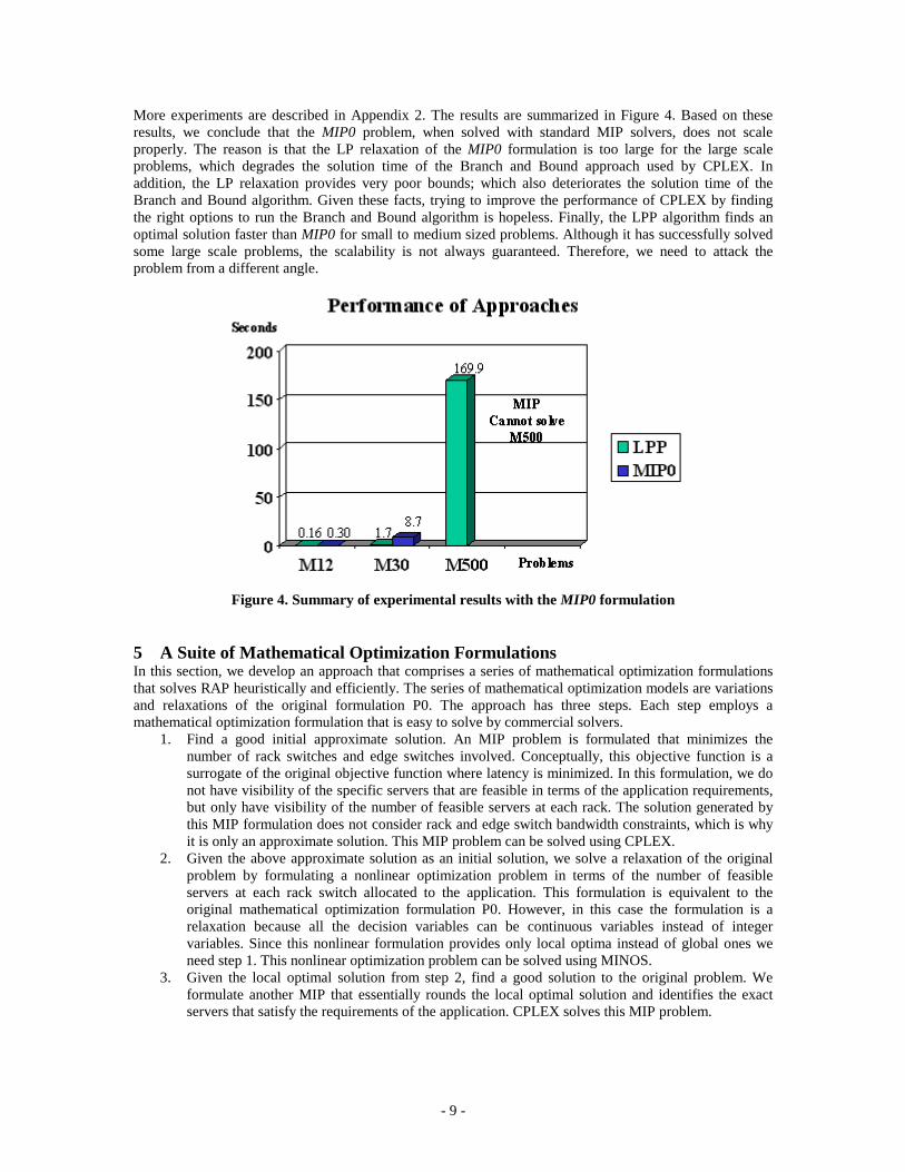
More experiments are described in Appendix 2. The results are summarized in Figure 4. Based on these results, we conclude that the MIP0 problem, when solved with standard MIP solvers, does not scale properly. The reason is that the LP relaxation of the MIP0 formulation is too large for the large scale problems, which degrades the solution time of the Branch and Bound approach used by CPLEX. In addition, the LP relaxation provides very poor bounds; which also deteriorates the solution time of the Branch and Bound algorithm. Given these facts, trying to improve the performance of CPLEX by finding the right options to run the Branch and Bound algorithm is hopeless. Finally, the LPP algorithm finds an optimal solution faster than MIP0 for small to medium sized problems. Although it has successfully solved some large scale problems, the scalability is not always guaranteed. Therefore, we need to attack the problem from a different angle.

Figure 4. Summary of experimental results with the MIP0 formulation

5 A Suite of Mathematical Optimization Formulations In this section, we develop an approach that comprises a series of mathematical optimization formulations that solves RAP heuristically and efficiently. The series of mathematical optimization models are variations and relaxations of the original formulation P0. The approach has three steps. Each step employs a mathematical optimization formulation that is easy to solve by commercial solvers.

1. Find a good initial approximate solution. An MIP problem is formulated that minimizes the number of rack switches and edge switches involved. Conceptually, this objective function is a surrogate of the original objective function where latency is minimized. In this formulation, we do not have visibility of the specific servers that are feasible in terms of the application requirements, but only have visibility of the number of feasible servers at each rack. The solution generated by this MIP formulation does not consider rack and edge switch bandwidth constraints, which is why it is only an approximate solution. This MIP problem can be solved using CPLEX.

2. Given the above approximate solution as an initial solution, we solve a relaxation of the original problem by formulating a nonlinear optimization problem in terms of the number of feasible servers at each rack switch allocated to the application. This formulation is equivalent to the original mathematical optimization formulation P0. However, in this case the formulation is a relaxation because all the decision variables can be continuous variables instead of integer variables. Since this nonlinear formulation provides only local optima instead of global ones we need step 1. This nonlinear optimization problem can be solved using MINOS.

3. Given the local optimal solution from step 2, find a good solution to the original problem. We formulate another MIP that essentially rounds the local optimal solution and identifies the exact servers that satisfy the requirements of the application. CPLEX solves this MIP problem.

- 10 -

We start with the nonlinear optimization formulation, step 2 of our approach, since this formulation is at the core of the solution approach. Then, we describe the MIP formulation that comprises step 3, which chooses the specific servers. Finally, we describe the MIP formulation in step 1, which determines good initial solutions for the nonlinear optimization problem. 5.1 QP (Step 2) --- Nonlinear Optimization and Binary Relaxation For combinatorial optimization problems with binary variables, it is sometimes advisable, if possible, to reformulate the problem in terms of continuous variables over an interval. This brings convexity to the formulation and helps the continuous relaxation to be stronger, which means that the relaxation will give tighter bounds. For this purpose, a quadratic programming approximation of the original problem is formulated, referred to as QP. The interested reader might consult the book written by Gill, Murray, and Wright [4] for a comprehensive description of the theory and practice of Non-linear Programming models. A new decision variable is defined as follows.

• lrxr : Number of feasible servers connected to rack switch r that are allocated to tier l.

• [ ]llr Nxr ,0∈ .

• For a given rack r, ∑∈

=rSRs

lslslr xFxr .

The variable lrxr appears in the QP formulation if and only if 1≥∑∈ rSRs

lsF , which means the rack switch r

has a feasible server for tier l. To simplify the notation, we define a new set SSRFSR rlr ⊂⊂ , which is

the set of servers connected to rack switch r that are feasible for tier l. We now reformulate each constraint

in the original problem P0 in terms of lrxr . The details of the formulation of the QP problem are explained

in Appendix 3. The resulting QP formulation follows.

)0(∑∑∑ ∑ ∑∑∑∈ ∈ ∈ ∈ ∈ ∈ ∈

+=Rr Li Ll Ee Rr Li Ll

irlrliirlrli

e

xrxrTxrxrTZQPMax

Subject to:

∑∈

∈=Rr

llr LlNxr )1( ,

Constraints (2). We assume a 3-tier architecture; extensions to other number of tiers can be easily considered. For all Rr ∈ ,

rlrlrlrlrlrl FSRFSRFSRxrxrxr 321321 ∪∪≤++

rlrlrlrl FSRFSRxrxr 2121 ∪≤+



rlrl FSRxr 110 ≤≤ rlrl FSRxr 220 ≤≤ rlrl FSRxr 330 ≤≤

)6( , RrBROxrxrTxrTO rLl Li Ll

irlrlilrl ∈≤−∑ ∑∑∈ ∈ ∈

)7( , RrBRIxrxrTxrTI rLl Li Ll


∑∑ ∑ ∑∑∑∈ ∈ ∈ ∈ ∈ ∈

∈≤−e e eRr Ll Rq Rr Li Ll

eiqlslilrl EeBEOxrxrTxrTO )8( ,

∑∑ ∑ ∑∑∑∈ ∈ ∈ ∈ ∈ ∈


eiqlslilrl EeBEIxrxrTxrTI )9( ,

∑∈

≥∋∈∈≥rSRs

lslr FRrLlxr 1 , ,0

- 11 -

Experimental results with the QP model are presented in Appendix 4. We note that the QP model is significantly smaller than the LP relaxation of the MIP0. The QP model represents a promising approach since it can be solved very fast and finds the optimal solution in terms of the xr variables if a good initial solution is provided. 5.2 MIP2 (Step 3) --- Intelligent Rounding In this section, we formulate a Mixed Integer Programming problem, MIP2, to intelligently round the local optimal solution generated by the QP model. The MIP2 model defines the actual servers to allocate to the application. The decision variables are the same as those in the original problem P0.

=otherwise

ltiertoassignedsserverxls 0

1

The first two constraints of the model are similar to those for the P0 problem.

∑∈

∈=Ss

lls LlNx )1( ,

)2( ,1 SsxLl

ls ∈≤∑∈

For each rack switch r and tier l, allocate as many servers as recommended by the local optimal solution, *xr , from the QP model.

)3(0 if ** >≥∑∈

lrSRs

lrls xrxrxr

As we have explained, constraints (3), (4) and (5) of the original problem P0 are captured by the feasibility

matrix F. Accordingly, we impose another constraint },0{ lsls Fx ∈ to ensure that the variable lsx appears

in the formulation if and only if 1=lsF . Incoming and outgoing bandwidth capacity constraints are not

considered because these constraints are satisfied by the solution of the QP model. The MIP2 model is just rounding the QP solution without modifying total traffic going through rack switches and edge switches. The objective function is simply to minimize the number of servers allocated.

∑∑∈ ∈Ll Ss

lsxMin )0(

Observe that the above objective function is a constant, ∑∈ Ll

lN , due to constraint (1). The reason why it is

imposed is not that the rounding model needs it. Instead, it is because the commercial solver that we use for mixed integer programming requires that an objective function be specified. Due to the fact that all feasible solutions have the same objective function value, the minimization does not enforce anything, which is what we want in this case. In some other cases, we might want to use the objective function to minimize the total “cost” of allocating servers to the application. In summary, the MIP2 formulation is as follows.

∑∑∈ ∈Ll Ss

lsxMin )0(

Subject to

∑∈

∈=Ss

lls LlNx )1( ,

)2( ,1 SsxLl

ls ∈≤∑∈

)3(0 if ** >≥∑∈

lrSRs

lrls xrxrxr

{ }lsls Fx ,0∈

- 12 -

This formulation is like a transportation model with side constraints. The CPLEX solver exploits this structure nicely and solves it extremely fast. 5.3 MIP0 (Step 1) --- Initial Solution As we observed from the experiments of the QP model, this model needs a good starting solution to find the global optimal solution, or at least a good local optimum for the original problem P0. Recall that the initial solution for the QP model does not need to be feasible. Hence, in this section, we formulate a Mixed Integer Programming problem, MIP1, to generate a good initial solution for the QP model. The MIP1 formulation is based on the following intuitions. First, if there is a feasible server assignment under a single rack switch that satisfies constraints (1) to (5) of the original problem P0, then this solution is most likely feasible for the rack and edge switches bandwidth constraints (6) to (9). Second, this feasible server assignment is optimal for P0. This is easy to show. From appendix 1, the objective function of P0 is formulated as minimizing the weighted average of the number of hops between each pair of servers, i.e.,

MER FFFzMin 642 ++=�,

where MER FFF and , are the total amounts of inner traffic at all rack switches, edge switches and mesh

switch, respectively. In addition, ∑∑∈ ∈

=++Ll Li

ililMER NTNFFF , which is a constant. Let it be

denoted by C. Hence, ME FFCz 422ˆ ++= . Since 0≥EF and 0≥MF , we have Cz 2ˆ ≥ . The

optimum is achieved if and only if CF R = and 0== ME FF , which is exactly the case when only servers under one rack switch are chosen. Furthermore, even if more than one rack switches are needed, the

intention will be to minimize ME FF and as much as possible. Observer that EF is larger when more

rack switches are involved, and MF is larger when more edge switches are involved. Therefore, the main idea in the MIP1 model is to try to allocate servers that are in the same rack or that are in “closer” racks, where two racks are considered to be close if they are connected to the same edge switch. It would be desirable for each rack switch to have an “appropriate server mix” so that an application with “typical” server requirements can be hosted using a single rack switch or a minimum number of rack switches. A related tactical optimization problem would be to identify such server mix for a set of applications. On the other hand, data center operators may prefer the idea of having the same kind of servers under each rack switch for easy maintenance. Based on the above discussion, the objective function of the MIP1 formulation is a surrogate function of the objective function of P0. Roughly speaking, the objective of MIP1 is to minimize the total weighted usage of rack and edge switches. Consequently, the MIP1 problem is formulated as a “Facility Location Optimization Problem”. We define the following “location” variables:

=∈otherwise

usediseswitchedgeifuEeeachFor e 0

1,

=∈otherwise

usedisrswitchrackifvRreachFor r 0

1,

The weights for these location variables are chosen so that the minimization of the objective function emulates the direction of optimality in the original problem P0. In particular, we define the weight for each switch used to be the latency measure (number of hops) for that switch, i.e., 2=rCR , and 4=eCE .

The main issue with the original formulation P0 is that we have a combinatorial optimization problem with binary variables, quadratic constraints, and a quadratic objective function. Having removed the nonlinearity from the objective function in MIP1 already, we would further remove the quadratic bandwidth constraints for rack and edge switches to linearize the problem. Therefore, the MIP1 formulation is an approximation of the original problem P0. It is not guaranteed to generate a feasible solution for P0.

- 13 -

However, this is acceptable since the goal of the MIP1 model is to generate good initial solutions for the QP model, which explicitly considers the quadratic constraints removed in the MIP1 formulation. As in the QP model, we assume a 3-tier architecture for the application. Extensions to other number of tiers

are easy to implement. Similar to the QP formulation, we define lrx as the number of feasible servers in

rack switch r allocated to tier l. The lrx appears in the formulation if and only if rack switch r has a

feasible server for tier l. The constraints of the MIP1 formulation are as follows.

Constraint 1) The total number of servers allocated to tier l is lN .

∑∈

∈=Rr

llr LlNxr )1( ,

Constraint 2) Allocate at most one server to a tier and ensure that no server allocated is double counted.





rlrl FSRxr 110 ≤≤ , rlrl FSRxr 220 ≤≤ , rlrl FSRxr 330 ≤≤

Constraint 3) These are logical constraints over the binary variables eu and rv that ensure that these

variables behave as intended. If we want to allocate servers from rack switch r to tier l then rack switch r needs to be “used”. That is,

1. 1=rv if 0>lrxr ;

2. 0=rv if 0=lrxr .

Therefore, we define the following constraint:

)1.3( , ∅≠≥ lrlrrl FSRxrvN

Where the coefficient of the variable rv is an upper bound of the variable lrxr . Note that condition 1 is

satisfied by constraint (3.1), and condition 2 is satisfied by this constraint and because we are minimizing

the weighted summation of rv variables, at optimality 0=rv if 0=lrxr .

Now, if we want to “use” rack switch r, we need to “use” the edge switch e connected to this rack switch. That is,

1. 1=eu if 1=rv ;

2. 0=eu if 0=rv .

Hence, we define the following constraint: )2.3( , , ere RrEevu ∈∈≥

This constraint ensures condition 1 is satisfied, and condition 2 is satisfied at optimality. The objective function of the MIP1 formulation is to minimize the total cost of “using” rack and edge switches, and is defined as follows

)0( ∑∑∈∈

+Rr

rrEe

ee vCRuCEMin

In summary, the formulation of the MIP1 model is

)0( ∑∑∈∈

+Rr

rrEe

ee vCRuCEMin

Subject to:

- 14 -

∑∈

∈=Rr

llr LlNxr )1(,





rlrl FSRxr 110 ≤≤ , rlrl FSRxr 220 ≤≤ , rlrl FSRxr 330 ≤≤

)1.3( , ∅≠≥ lrlrrl FSRxrvN

)2.3( , , ere RrEevu ∈∈≥

{ }∑∈

≥×∈≥∈∈∈

rSRslsls

re

FRLrlxr

RrEevu

1 and ,, ,0

,,1,0,

This type of “Facility Location” formulation has a structure that CPLEX can exploit very effectively and can be solved extremely fast. 6 Experimental Results of the MP Approach This section summarizes the Mathematical Programming (MP) approach we have developed to tackle the resource allocation problem P0 and shows some experimental results. The MP approach involves three steps. Each step represents a mathematical optimization formulation that is easy to solve using commercial solvers.

1. Generate a good initial approximate solution 0lrxr for the QP model using the MIP1 formulation,

which can be solved efficiently by CPLEX.

2. Use the approximate solution 0lrxr as an initial solution for the QP problem; use MINOS as the

solver to find a local optimal solution of the QP problem, *lrxr . We expect that this local optimal

solution would be a global optimal solution or a good local optimal solution.

3. With the local optimal solution *lrxr of the QP problem, use the MIP2 formulation to identify the

specific servers to be allocated to each tier in the application, *lsx . CPLEX solves the MIP2

problem very fast. Both the MP approach and the LPP algorithm were applied to a set of problems of different sizes to compare the performance. The problems were divided into two sets, one with 500 servers and the other with 1000 servers. Within each set, a few other parameters were varied to influence the complexity of the problem, such as the number of servers required in each tier of the application, the numbers of edge and rack switches, and the amount of incoming or outgoing bandwidth at the edge and rack switches. From each set, three problems are chosen as representatives and the results are summarized in Table 4. Due to the fact that the two algorithms were running on different kinds of machines, the comparison of the absolute numbers for computation time is less meaningful than the variance between different problems. The same data is presented graphically in Figure 5. It is easy to see that the solution time of the LPP algorithm heavily depends on the parameters of the problem, while the performance of the MP approach is much more stable, especially within problems of the same server number. Overall the MP approach is more robust and scalable and is able to find good solutions quickly when the problem is feasible and not too tight in terms of the rack and edge switch bandwidth constraints. However, when the problem is tight, the MP approach is not very reliable, since it may declare the problem infeasible while in fact there exist feasible solutions. On the other hand, the LPP algorithm is in favor of tighter problems, because its efficiency relies on the ability to quickly prune infeasible nodes in the search tree, which is easier when the bandwidth

- 15 -

constraints are tighter. Consequently, a hybrid MP and LPP approach is desirable, where the LPP approach is used to determine infeasibility or identify a good feasible solution whenever the MP approach fails to find a feasible solution. This hybrid method will be described in the next section.

Table 4. Comparison between the LPP and MP approaches

Figure 5. Comparison of the LPP and MP approaches

- 16 -

Another advantage of the MP approach is that it can be extended to handle more general problems that capture the operational issues and economical factors inherent in the management of large IDCs (e.g., 50,000 servers). These extensions do not require the invention of new algorithms. Instead, the new problems need to be formulated in an intelligent way such that they can be efficiently solved using existing commercial solvers. 7 A Hybrid MP and LPP approach In this section, we describe a hybrid MP and LPP approach to tackle the RAP. Please refer to Figure 6 to follow the flow of events of the hybrid approach.

1. The approach requires the following inputs a. Resource physical topology and capacities. b. Application architecture and resource requirements.

2. The “Facility Location” surrogate problem, MIP1, is solved to generate a “good” initial solution. 3. Given the initial solution generated by MIP1, a relaxation problem QP is solved. 4. The solution of the QP model can either be a local optimum or infeasible.

a. If the solution of QP is infeasible, then the LPP algorithm is used to determine if the original problem P0 is feasible or not. If a feasible solution is found, go to 5; otherwise,

i. if the LPP algorithm declares the original problem P0 as infeasible, then solve a feasibility model, which is a variation of the relaxation problem QP. The purpose of this feasibility model is to identify which rack and/or edge switches need to increase the bandwidth and the amount of this increase. We refer to this feasibility model as the FModel. The FModel adds artificial variables to the incoming/outgoing bandwidth constraints to the QP model and minimizes the sum of these artificial variables. If bandwidth is increased as recommended by the FModel, then go to 1, and resolve the revised model.

b. If the solution of QP is a local optimum, then solve the intelligent rounding problem, MIP2. The solution of MIP2 is a feasible solution of the original problem P0.

5. Implement the feasible solution found. 8 Future Research The following extensions to RAP and some related topics will be explored in our future research.

1. The RAP studied in this paper employs a multi-tier architecture for applications. Although the multi-tier configuration is fairly common in current Web applications, there are applications that do not necessarily require a tiered structure. We are formulating a mathematical optimization model for general distributed applications that require a set of communicating servers.

2. We have taken the approach of allocating resources to one application at a time, which provides a suboptimal solution to efficiently sharing resources by multiple applications. It will be interesting to explore the formulation of RAP when multiple applications are considered simultaneously.

3. It is also desirable to consider general network topologies that do not have a hierarchical tree structure.

4. Capacity at IDCs can be expanded by scaling out – adding more servers of the same type, or scaling up – upgrading current servers by installing latest software or adding hardware components. We are working on a model that will capture the cost trade-off between scaling out and scaling up.

5. We are investigating a methodology that may further substantiate the notions of “Intelligent Provisioning” and “Capacity on Demand” which allows to integrate demand planning – workload management at IDCs, with capacity planning – optimal resource allocation to satisfy dynamic application requirements. For more details see Garg et al [3].

6. We attempt to use mathematical programming approaches for more systematic return on investment (ROI) and total cost of ownership (TCO) analysis for IDCs. For more details see Crowder et al [2].

- 17 -

Figure 6. Flow Diagram of the hybrid MP & LPP approach

4. Is QP solution Feasible?

2. Solve MIP1 Facility Location Problem

Initial Solution

3. Solve QP Relaxation of P0

4a. Solve using LPP algorithm

NO

YES

Is LPP solution Feasible?

4b. Solve MIP2 Intelligent Rounding

NO

4a.i. Solve FModel Feasibility Model

Recommendations for Resource Capacity Change

5. Implement Feasible Solution

YES

1a. Resource Physical Topology Resource Capacities

1b. Application Architecture Resource Requirements

- 18 -

Bibliography 1. K. Appleby, S. Fakhouri, L. Fong, G. Golszmidt, M. Kalantar, S. Krishnakumar, D.P. Pazel, J.

Pershing and B. Rockwerger. “Océano–SLA based management of computing utility,” Proceedings of 2001 IEEE/IFIP International Symposium on Integrated Network Management (IM 2001), Seattle, May 2001.

2. H. P Crowder, P. K. Garg, C. A Santos and X. Zhu. “UDC Financial Planning (UFP)”. Power point presentation, December 7, 2001.

3. P. K Garg, Ming Hao, C. A Santos, H. K. Tang, A. X. Zhang. “Web Transaction Analysis and Optimization (TAO),” working paper.

4. P. E. Gill, W. Murray and M. H. Wright. Practical Optimization, Academic Press, 1981. 5. J. Rolia, S. Singhal and R. Friedrich, “Adaptive Internet Data Centers,” Proceedings of SSGRR

2000 Computer and eBusiness Conference, L'Aquila, Italy, July-August, 2000. 6. L. A. Wolsey. Integer Programming, Wiley, 1998. 7. X. Zhu and S. Singhal. "Optimal Resource Assignment in Internet Data Centers," Proceedings of

the Ninth International Symposium on Modeling, Analysis, and Simulation of Computer and Telecommunications Systems, pp. 61-69, Cincinnati, Ohio, August 2001. http://www.hpl.hp.com/personal/Sharad_Singhal/Zhu_Mascots2001.pdf

- 19 -

Appendix 1 Mathematical Formulation of P0 This appendix contains details of the development of the constraints and the objective function of P0. The following constraints are posed on the decision variables.

• The total number of servers allocated to tier l is lN :

∑∈

∈=Ss

lls LlNx )1( ,

• Each server in the physical topology can only be assigned no more than once to a particular tier:

)2( ,1 SsxLl

ls ∈≤∑∈

• The attribute values for each server assigned satisfy the minimum and maximum requirements:

)3( , , SsAaxVMAXVxxVMINLl

lslaasLl

lsLl

lsla ∈∈≤

≤ ∑∑∑

∈∈∈

Note that the summation ∑∈ Ll

lsx is either 0 or 1, because of constraint (2) and the terms in the summation

are binary variables. Therefore, constraint (3) takes the following forms for any feasible solution:

000 ≤≤≤≤ orVMAXVVMIN lalala .

• The outgoing and incoming bandwidth constraints for all the links that connect the servers to the rack

switches are:

)4( , SsBSOxTO sLl

lsl ∈≤∑∈

)5( , SsBSIxTI sLl

lsl ∈≤∑∈

Since the summation ∑∈ Ll

lsx is either 0 or 1, then constraint (4) takes the following values for any feasible

solution: 00 ≤≤ orBSOTO sl . The same argument can be given for constraint (5). Therefore constraints

(4) and (5) force the traffic at the server assigned to a tier to satisfy the server outgoing or incoming bandwidth requirement for that tier. • The outgoing and incoming bandwidth constraints for all the links that connect the rack switches to the

edge switches are:

)6( , RrBROxxTxTO rSRj Li Ll SRs

ijlsliLl SRs

lsl

r rr

∈≤− ∑ ∑∑ ∑∑ ∑∈ ∈ ∈ ∈∈ ∈

)7( , RrBRIxxTxTI rSRj Li Ll SRs

ijlsliLl SRs

lsl

r rr

∈≤− ∑ ∑∑ ∑∑ ∑∈ ∈ ∈ ∈∈ ∈

Consider constraint (6). For each tier l and rack switch r, define ∑∈

=rSRs

lslr xxr as the number of servers

under rack switch r allocated to tier l. Then, the outgoing traffic at rack switch r is the total amount of

outgoing traffic generated by all the connected servers under this switch, ∑ ∑∈ ∈Ll SRs

lsl

r

xTO , reduced by the

amount of inner traffic6 at this switch, ∑ ∑∑ ∑∈ ∈ ∈ ∈r rSRj Li Ll SRs

ijlsli xxT . At the same time, the outgoing traffic at

rack switch r should be less than the rack switch’s outgoing bandwidth. The same reasoning can be given for constraint (7). 6 Inner traffic at a particular switch is defined as the sum of traffic between any pair of servers connected by this same switch.

- 20 -

• The outgoing and incoming bandwidth constraints for all the links that connect the edge switches to the mesh switches are:

)8( , EeBEOxxTxTO eSEj Li Ll SEs

ijlsliLl SEs

lsl

e ee

∈≤− ∑ ∑∑ ∑∑ ∑∈ ∈ ∈ ∈∈ ∈

)9( , EeBEIxxTxTI eSEj Li Ll SEs

ijlsliLl SEs

lsl

e ee

∈≤− ∑ ∑∑ ∑∑ ∑∈ ∈ ∈ ∈∈ ∈

Consider constraint (8). For each tier l and edge switch e, define ∑∈

=eSEs

lsle xxe as the number of servers

under edge switch e allocated to tier l. Then, the outgoing traffic at edge switch e is the total amount of

outgoing traffic generated by all the connected servers under this switch, ∑ ∑∈ ∈Ll SEs

lsl

e

xTO , reduced by

amount of inner traffic at this switch, ∑ ∑∑ ∑∈ ∈ ∈ ∈e eSEj Li Ll SEs

ijlsli xxT . At the same time, the outgoing traffic at

edge switch e should be less than the edge switch’s outgoing bandwidth. The same reasoning can be given for constraint (9). The objective of the optimization problem is to minimize the communication delay between servers for each set of application requirements. Consider the number of hops7 needed for two servers to communicate.

Consider the case when the physical topology is a hierarchical tree. Define RF as the total traffic between

all the server pairs that communicate only through a rack switch. That is, RF is the sum of the inner traffic

for each rack switch r, ∑ ∑∑ ∑∈ ∈ ∈ ∈r rSRj Li Ll SRs

ijlils xTx . Therefore,

∑ ∑ ∑∑ ∑∈ ∈ ∈ ∈ ∈

=Rr SRj Li Ll SRs

ijlilsR

r r

xTxF .

Define NHR as the number of hops needed for two servers under the same rack switch to communicate. Note that NHR=2.

Define EF as the total traffic between all the server pairs that have to communicate through an edge

switch. That is, EF is the sum of the inner traffic for each edge switch e, ∑ ∑∑ ∑∈ ∈ ∈ ∈e eSEj Li Ll SEs

ijlils xTx ,

reduced by the traffic that only goes through a rack switch, RF . Consequently,

∑ ∑ ∑∑ ∑∈ ∈ ∈ ∈ ∈

−=Ee SEj Li Ll SEs

Rijlils

E

e e

FxTxF .

Define NHE as the number of hops needed for each data packet between two servers to go through an edge switch. Observe that NHE=4.

Define MF as the total traffic between all the server pairs that have to communicate through a mesh

switch. That is, MF is the total traffic between all the server pairs, ∑∑∈ ∈Ll Li

ilil NTN , reduced by the sum of

the inner traffic at all the edge switches. Consequently,

∑ ∑ ∑∑ ∑∑∑∈ ∈ ∈ ∈ ∈∈ ∈

−=Ee SEj Li Ll SEs

ijlilsLl Li

ililM

e e

xTxNTNF .

Define NHM as the number of hops needed for each data packet between two servers to go through a mesh switch. Note that NHM=6.

7 The number of hops is defined as the number of arcs in the path of minimal length that connects two servers in the graph that represents the physical topology.

- 21 -

We now have defined all the terms that determine the objective function. Therefore, if we want to minimize the communication delay between servers for each set of application requirements, the objective function of the optimization model is to minimize the average number of hops for each server pair weighted by the corresponding amount of traffic between these two servers. That is,

MER FNHMFNHEFNHRMin *** ++ .

Substituting and canceling terms, we have

ijEe SEj Li Ll SEs

lilsRr SRj Li Ll SRs

ijlilsLl Li

ilil xTxxTxNTNzMine er r

∑ ∑ ∑∑ ∑∑ ∑ ∑∑ ∑∑∑∈ ∈ ∈ ∈ ∈∈ ∈ ∈ ∈ ∈∈ ∈

−−= 226�

The first term is a constant, so it can be ignored from the optimization model. Therefore, instead of minimize z

�, we can maximize z, where

ijEe SEj Li Ll SEs

lilsRr SRj Li Ll SRs

ijlils xTxxTxzMaxe er r

∑ ∑ ∑∑ ∑∑ ∑ ∑∑ ∑∈ ∈ ∈ ∈ ∈∈ ∈ ∈ ∈ ∈

+=

Appendix 2 Experimental Results of the MIP0 Model In this Appendix, we present the experimental results of using the MIP0 formulation. First a problem called “M30” with 30 servers was tested. The global parameters for this problem are:

• Five attributes per server • Six edge switches • Two rack switches • Three tiers • The server requirements by the application are N = (4,5,3). • The MIP0 formulation has the following dimensions:

o 1682 equations o 526 non-negative continuous variables y o 50 binary variables x

• The model can be solved in 8.7 seconds with GAMS (MIP0) /CPLEX7.0 • The LPP algorithm developed by Zhu and Singhal takes 1.7 seconds. • The optimal solution value found by both approaches is 17.2.

Then a problem called “M500” with 500 servers was tested. The global parameters for this problem are:

• Five attributes per server • Five edge switches • Number of rack switches is 25 • Three tiers • The server requirements by the application are N = (6, 8, 5).

The LPP algorithm can solve this problem optimally in 169.9 sec. The optimal objective function found is 62.4. The servers in the solution are all in rack switch r18. The servers in

• Tier 1 are (s341, s342, … , s346) • Tier 2 are (s347, … , s354) • Tier 3 are (s355, … ,s359)

The MIP0 problem has about 810 binary variables x and about 57,800 continuous variables y.

The Linear Programming Relaxation ( )10 ≤≤ x has the following properties:

• 179,000 equations • 58,610 variables • 560,000 non-zero coefficients • This relaxation solves using GAMS/CPLEX6.0 Primal Simplex in about 17 min 35 sec. • This relaxation solves using GAMS/CPLEX6.0 Dual Simplex in about 5 min 18 sec. • This relaxation is too big, and solves too slowly.

- 22 -

• The optimal objective function value of the relaxation is 264. • The LP relaxation gives poor bounds (264/62.4 = 4.23). It seems the y variables lose their meaning

as a product of 2 binary variables, when x is no longer binary but continuous in the interval [0,1]. • The MIP0 problem itself cannot be solved by GAMS/CPLEX6.0 after running for almost a week.

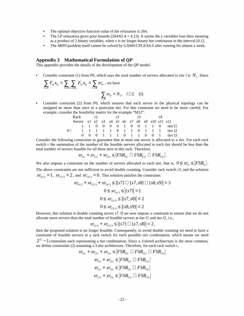
Appendix 3 Mathematical Formulation of QP This appendix provides the details of the development of the QP model.

• Consider constraint (1) from P0, which says the total number of servers allocated to tier l is lN . Since

∑ ∑ ∑ ∑∈ ∈ ∈ ∈

==Ss Rr SRs Rr

lrlslslsls

r

xrxFxF , we have

∑∈

∈=Rr

llr LlNxr )1( ,

• Consider constraint (2) from P0, which ensures that each server in the physical topology can be assigned no more than once to a particular tier. For this constraint we need to be more careful. For example, consider the feasibility matrix for the example “M12”.

Rack r1 r2 r3 r4 Server s1 s2 s3 s4 s5 s6 s7 s8 s9 s10 s11 s12

1 1 0 0 0 0 1 0 0 1 1 0 tier l1 F= 1 1 1 1 1 0 1 1 0 1 1 1 tier l2

0 0 0 1 1 1 0 1 1 0 0 1 tier l3 Consider the following constraints to guarantee that at most one server is allocated to a tier. For each rack switch r the summation of the number of the feasible servers allocated to each tier should be less than the total number of servers feasible for all three tiers in this rack. Therefore,

rlrlrlrlrlrl FSRFSRFSRxrxrxr 321321 ∪∪≤++ .

We also impose a constraint on the number of servers allocated to each tier, that is, lrlr FSRxr ≤≤0 .

The above constraints are not sufficient to avoid double counting. Consider rack switch r3, and the solution

131 =rlxr , 232 =rlxr , and 033 =rlxr . This solution satisfies the constraints

3}9,8{}8,7{}7{333231 =∪∪≤++ sssssxrxrxr rlrlrl

1}7{0 31 =≤≤ sxr rl

2}8,7{0 32 =≤≤ ssxr rl

2}9,8{0 33 =≤≤ ssxr rl

However, this solution is double counting server s7. If we now impose a constraint to ensure that we do not allocate more servers than the total number of feasible servers at tier l1 and tier l2, i.e.,

2}8,7{}7{3231 =∪≤+ sssxrxr rlrl ,

then the proposed solution is no longer feasible. Consequently, to avoid double counting we need to have a constraint of feasible servers at a rack switch for each possible tier combination, which means we need

12 || −L constraints each representing a tier combination. Since a 3-tiered architecture is the most common, we define constraints (2) assuming a 3-tier architecture. Therefore, for each rack switch r,





- 23 -

rlrl FSRxr 110 ≤≤



• Constraints (3), (4) and (5) from P0 are omitted because they are implicitly considered in the

generation of the variables lrxr .

• The outgoing and incoming bandwidth constraints for all the links that connect the rack switches to the edge switches are represented by constraints (6) and (7) from P0. Consider the first term of constraint (6),

∑ ∑ ∑ ∑∑∈ ∈ ∈ ∈∈

==Ll SRs Ll Ll

lrlSRs

lslsllsl

r r

xrTOxFTOxTO .

Now consider the second term of constraint (6),

∑∑ ∑∑ ∑ ∑ ∑ ∑∈∈ ∈ ∈ ∈ ∈ ∈ ∈

==Lil

irlilsSRj Li Ll SRs Lil SRs SRj

ijijlslsliijlsli xrTxrxFxFTxxTr r r r ,,

.

Constraints (7) can be treated in a similar manner. Therefore we have constraints (6) and (7) defined in

terms of lrxr as follows.

)6( , RrBROxrxrTxrTO rLl Li Ll


)7( , RrBRIxrxrTxrTI rLl Li Ll


• The outgoing and incoming bandwidth constraints for all the links that connect the edge switches to the mesh switches are represented by constraints (8) and (9) from P0. Consider the first term of constraint (8),

∑ ∑ ∑ ∑ ∑∑ ∑∈ ∈ ∈ ∈ ∈∈ ∈

==Ll SEs Ll Ll Rr

lrlRr SRs

lslsllsl

e ee r

xrTOxFTOxTO

Now consider the second term of constraint (8),

∑ ∑∑ ∑∑ ∑ ∑ ∑ ∑ ∑ ∑∈ ∈∈ ∈ ∈ ∈ ∈ ∈ ∈ ∈ ∈

==Lil Rqr

iqlrliSEj Li Ll SEs Lil Rr SRs Rq SRj

ijijlslsliijlsli

ee e e r e q

xrxrTxFxFTxxT, ,,

Constraints (9) can be treated in a similar fashion. Consequently, we have constraints (8) and (9) defined in

terms of lrxr as follows.

∑∑ ∑ ∑∑∑∈ ∈ ∈ ∈ ∈ ∈


eiqlslilrl EeBEOxrxrTxrTO )8( ,

∑∑ ∑ ∑∑∑∈ ∈ ∈ ∈ ∈ ∈


eiqlslilrl EeBEIxrxrTxrTI )9( ,

• Similarly, the objective function reformulated in terms of lrxr follows:

)0(∑∑∑ ∑ ∑ ∑∑∑∈ ∈ ∈ ∈ ∈ ∈ ∈ ∈

+=Rr Li Ll Ee Rq Rr Li Ll

iqlsliirlrli

e e

xrxrTxrxrTZQPMax

Appendix 4 Experimental Results of the QP model In this appendix we present the experimental results for the QP model. For the problem “M12”:

• The initial solution for the QP model is xr0 = 0. • The server requirements by the application are N=(2,2,1). • 32 equations • 11 variables

- 24 -

• 91 Non-zero coefficients • 50 Non-linear coefficients • The QP model local optimal solution is

o 3.3* =ZQP .

o 1,1,1,2 *23

*22

*12

*11 ==== rlrlrlrl xrxrxrxr .

o Solution time is 0.2 sec. • In this case, the QP model using GAMS/MINOS5.5 found the global optimal solution in terms of

variables xr, using xr0 = 0 as an initial solution. For the problem “M30”:

• The initial solution for the QP model is xr0=0. • The server requirements by the application are N=(4, 5, 3). • 43 equations • 15 variables • 127 non-zero coefficients • 68 non-linear coefficients • The QP model local optimal solution is

o 5.15* =ZQP , NOT a global optimal since the value of the optimal solution is 17.2.

o 3,2,3,1,3 *33

*32

*22

*21

*11 ===== rlrlrlrlrl xrxrxrxrxr .

o Solution time is 0.2 sec. • In this case, the QP model using GAMS/MINOS5.5 found a local optimal solution using xr0 = 0

as initial solution.

• Another initial solution was tested8, where xr is equal to its upper bound, that is ),( qixiq = .

o The QP model local optimal value is 1.17* =ZQP , and takes 0.2 sec to find it.

• We observed that the QP model is very sensitive to the initial solution provided. For the problem “M500”, which cannot be solved using the MIP0 formulation.

• The initial solution for the QP model is xr0=0. • The server requirements by the application are N= (6,8,5). • 149 equations • 45 variables • 397 non-zero coefficients • 202 non-linear coefficients • Observe that instantiation of the QP model for this problem is significantly smaller than the LP

relaxation of the MIP0 formulation. • The QP model local optimal value is

o 4.50* =ZQP , locally infeasible !!!

o Solution time is 2.6 sec.

• Another initial solution was tested, where xr is equal to its upper bound, that is lrlr FSRx = .

o The QP model local optimal value is 3.30* =ZQP . The optimal value found by the

LPP algorithm is 62.4. o Solution time is 2.6 sec.

• If instead, llr Nx =18 , the solution found by the LPP algorithm, was used as an initial solution for

the QP model, then

o The QP model local optimal value is 4.62* =ZQP .

o Solution time 2.6 sec.

8 Note that the initial solution for the QP model does not need to be feasible.

a mathematical optimization approach for resource ... · a mathematical optimization approach for...

Documents