Mathematical Optimization: introduction

Carlo Mannino

University of Oslo, INF-MAT5360 - Autumn 2011 (Mathematical optimization)

Practical Information

Lecturer: Carlo Mannino, mannino@dis.uniroma1.it

2 to 4 obligatory projects (assignments)

Written exams (theoretical arguments from the lectures, exercises (including, possibly, short proofs of properties).

Structure of the lesson

14:15 – 15:00 main topic

15:15 – 16 main topic

16:15 – 17 Exercises and questions (unless more time is needed)

Normally the lecture notes will be posted on the web-page the day before the lecture.

Reference Texts

Course Reference Texts:

Alexander Schrijver, A course in combinatorial optimization, http://homepages.cwi.nl/~lex/files/dict.pdf (Chap. 1)

Geir Dahl, Carlo Mannino, Notes on combinatorial optimization http://heim.ifi.uio.no/~geird/comb_notes.pdf

Geir Dahl, An introduction to convexity http://heim.ifi.uio.no/~geird/conv.pdf

Geir Dahl, Network flows and combinatorial matrix theory http://heim.ifi.uio.no/~geird/CombMatrix.pdf

Bradley, Hax, Magnanti, Applied Mathematical Programming http://web.mit.edu/15.053/www/AMP-Chapter-01.pdf

ILOG OPL Development Studio 5.5

Mathematical Models and Optimization

Mathematical Modelling

Model: a structure used to represent and analyze specific features or characteristics of concrete objects or systems

Mathematical Model: makes use of the algebraic formalism, i.e. variables, equations, inequalities, to represent concrete relations.

Good motives to build mathematical models:

- Mathematical analysis may reveal non-apparent properties

- Find quantitative solutions which may be used in practical decisions

- Allow for quick simulations (what-if scenarios)

Mathematical Optimization

Optimization Model: you want to find the best possible out of a set of feasible alternatives, according to some evaluation criterion

Mathematical Optimization Model: min {𝑐 𝑥 : 𝑥 ∈ 𝑆}

𝑐: 𝑆 → ℝ objective function, 𝑆 feasible solutions set

Typically S•⊆ ℝn is expressed by means of constraints, i.e.

𝑆 = 𝑥 ∈ ℝn: 𝑔𝑖 𝑥 ≤ 𝑏𝑖 , 𝑖 = 1, … , 𝑚 with 𝑔𝑖 : ℝ

n → ℝ

𝑔𝑖 , 𝑐 linear functions → linear programming (VS non-linear progr.)

and S ⊆ ℤ𝑛→ integer linear programming

|S| finite → combinatorial optimization

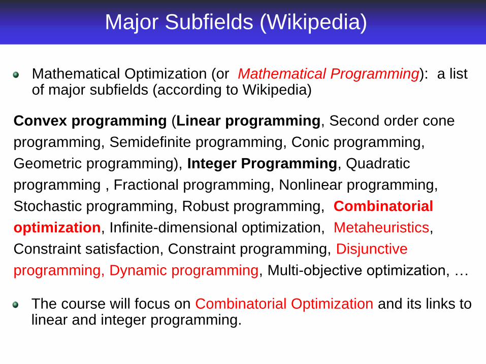
Convex programming (Linear programming, Second order cone

programming, Semidefinite programming, Conic programming,

Geometric programming), Integer Programming, Quadratic

programming , Fractional programming, Nonlinear programming,

Stochastic programming, Robust programming, Combinatorial

optimization, Infinite-dimensional optimization, Metaheuristics,

Constraint satisfaction, Constraint programming, Disjunctive

programming, Dynamic programming, Multi-objective optimization, …

Major Subfields (Wikipedia)

Mathematical Optimization (or Mathematical Programming): a list of major subfields (according to Wikipedia)

The course will focus on Combinatorial Optimization and its links to linear and integer programming.

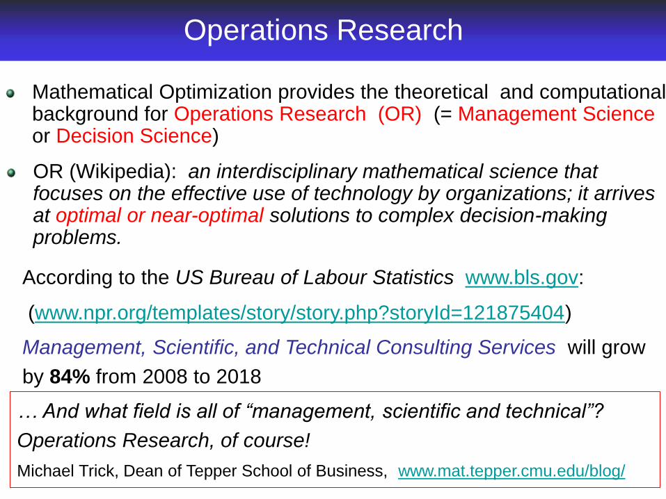
Mathematical Optimization provides the theoretical and computational background for Operations Research (OR) (= Management Science or Decision Science)

Operations Research

OR (Wikipedia): an interdisciplinary mathematical science that focuses on the effective use of technology by organizations; it arrives at optimal or near-optimal solutions to complex decision-making problems.

… And what field is all of “management, scientific and technical”?

Operations Research, of course!

Michael Trick, Dean of Tepper School of Business, www.mat.tepper.cmu.edu/blog/

Management, Scientific, and Technical Consulting Services will grow

by 84% from 2008 to 2018

According to the US Bureau of Labour Statistics www.bls.gov:

(www.npr.org/templates/story/story.php?storyId=121875404)

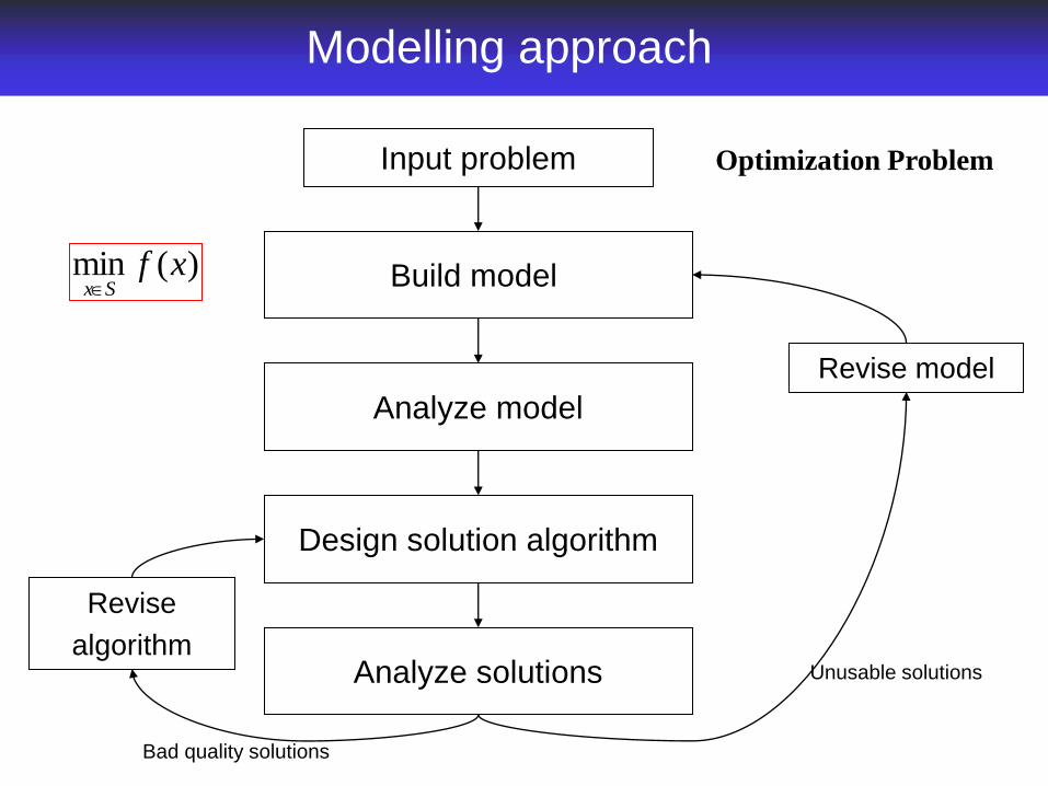
Input problem

Design solution algorithm

Analyze solutions

Revise

algorithm

Revise model

Analyze model

Build model

Optimization Problem

)(min xfSx

Modelling approach

Bad quality solutions

Unusable solutions

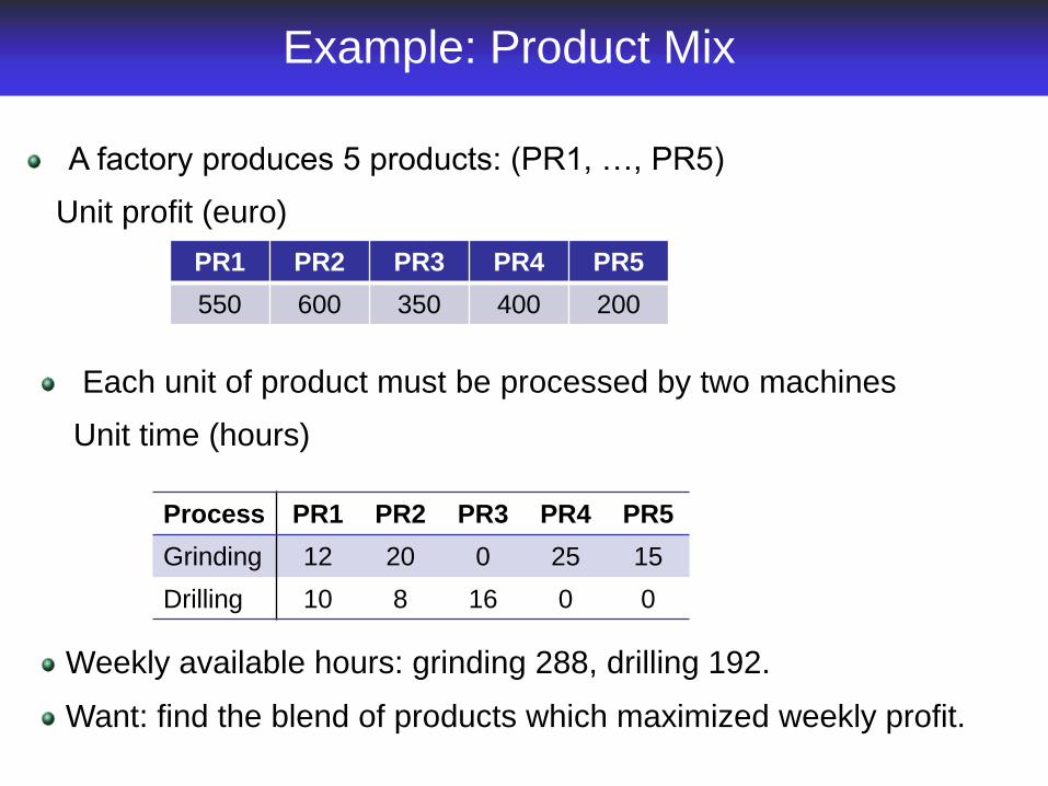
Example: Product Mix

A factory produces 5 products: (PR1, …, PR5)

PR1 PR2 PR3 PR4 PR5

550 600 350 400 200

Unit profit (euro)

Each unit of product must be processed by two machines

Unit time (hours)

Process PR1 PR2 PR3 PR4 PR5

Grinding 12 20 0 25 15

Drilling 10 8 16 0 0

Weekly available hours: grinding 288, drilling 192.

Want: find the blend of products which maximized weekly profit.

Product Mix: a linear program

Decision variables xi : quantity of PRi, i = 1, ….,5

Profit: 550 x1 + 600 x2 + 350 x3 + 400 x4 + 200 x5

Constraints: we cannot exceed grinding and drilling available hours

Grinding: 12 x1 + 20 x2 + 25 x4 + 15 x5 ≤ 288

Drilling: 10 x1 + 8 x2 + 16 x3 ≤ 192

𝑚𝑎𝑥 +550𝑥1 +600𝑥2 +350𝑥3 +400𝑥4 +200𝑥5

+12𝑥1 +20𝑥2 +25𝑥4 +15𝑥1 ≤ 288

+10𝑥1 +8𝑥2 +16𝑥3 ≤ 192

𝑥𝑖 ≥ 0 𝑖 = 1, … , 5

Canonical lp form: 𝑚𝑎𝑥 𝑐𝑇𝑥

𝐴𝑥 ≤ 𝑏𝑥 ≥ 𝑂

The complete LP-program:

Linear Programming: applications

There is a very large number of real-life problems that can be modeled by LP. Here is some examples

Petroleum Industry (refinery optimization problem)

Manufacturing Industry (lot sizing, stock control)

Transport, distribution, transhipment

Finance (portfolio optimization)

Energy

Defence

….

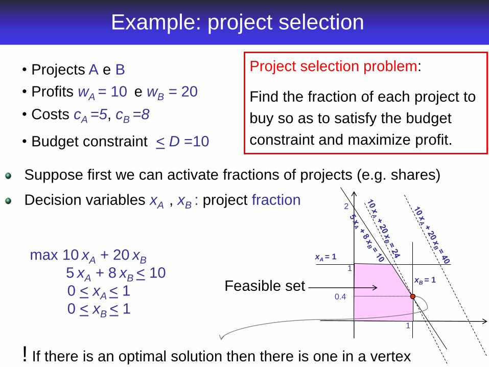
Example: project selection

• Projects A e B

• Budget constraint < D =10

• Costs cA =5, cB =8

Project selection problem:

Find the fraction of each project to

buy so as to satisfy the budget

constraint and maximize profit.

max 10 xA + 20 xB

5 xA + 8 xB < 10

0 < xA < 1

0 < xB < 1

• Profits wA = 10 e wB = 20

Suppose first we can activate fractions of projects (e.g. shares)

Decision variables xA , xB : project fraction

xA = 1

xB = 1

1

1

2

Feasible set 0.4

! If there is an optimal solution then there is one in a vertex

Example 0,1 LP: project selection

• Projects A e B

• Budget constraint < D =10

• Costs cA =5, cB =8

B

AS

1

0 ,

0

1 ,

0

0

Project selection problem:

Find a selection of projects

satisfying the budget constraint

and maximizing profit.

c({}) = 0, c({A}) = 5, c({B}) = 8,

c({A, B}) = 13 > D {A, B} not feasible

Feasible Solutions {{}, {A}, {B}}

xS

max 10 xA + 20 xB

S incident vectors of

the feasible solutions

• Profits wA = 10 e wB = 20

The problem can be written as a 0,1 linear program.

Solving 0,1 linear program is “difficult” (in general).

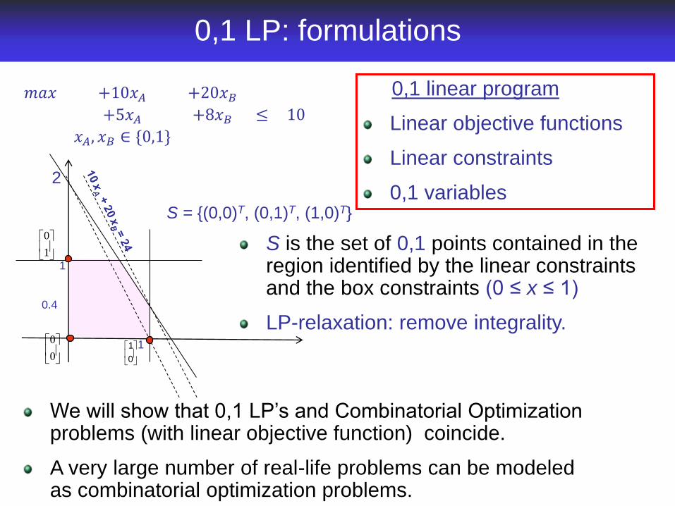
0,1 LP: formulations

S = {(0,0)T, (0,1)T, (1,0)T}

𝑚𝑎𝑥 +10𝑥𝐴 +20𝑥𝐵

+5𝑥𝐴 +8𝑥𝐵 ≤ 10

𝑥𝐴, 𝑥𝐵 ∈ {0,1}

We will show that 0,1 LP’s and Combinatorial Optimization problems (with linear objective function) coincide.

A very large number of real-life problems can be modeled as combinatorial optimization problems.

0

1

0

0

1

0

1

1

2

0.4

S is the set of 0,1 points contained in the region identified by the linear constraints and the box constraints (0 ≤ x ≤ 1)

LP-relaxation: remove integrality.

0,1 linear program

Linear objective functions

Linear constraints

0,1 variables

Combinatorial optimization: applications

17

Network design

Example: connectivity

You need to connect a source s (of

water, packets, …) to a number of

locations (farms, computers).

Each connection (pipe, fiber) has a cost

WANT: find a minimum cost network

connecting all locations to the source

s

2

3 7

5

2 1

3 s 11

20

1

7

1

4

s

18

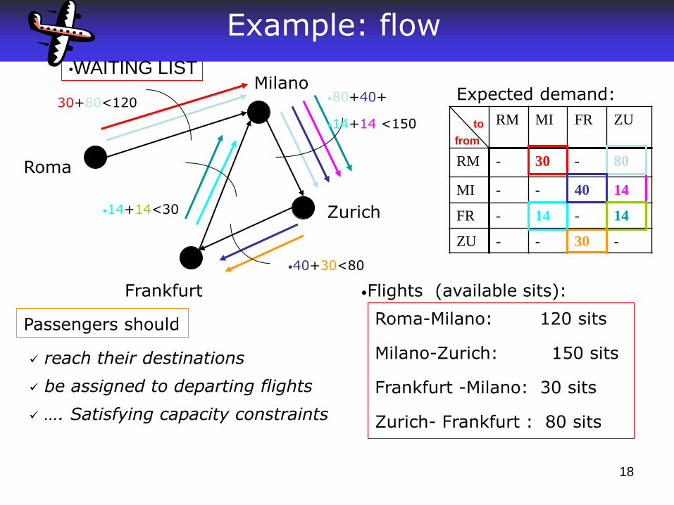
Example: flow

RM MI FR ZU

RM - 30 - 80

MI - - 40 14

FR - 14 - 14

ZU - - 30 -

Roma

Milano

Zurich

Frankfurt

Expected demand:

from

to

Roma-Milano: 120 sits

Milano-Zurich: 150 sits

Frankfurt -Milano: 30 sits

Zurich- Frankfurt : 80 sits

•Flights (available sits):

30+80<120 •80+40+

•14+14 <150

•14+14<30

•40+30<80

Passengers should

reach their destinations

be assigned to departing flights

…. Satisfying capacity constraints

•WAITING LIST

Example: Project Scheduling

1

4

2

3

6

8

5

1

0

7

9 SSmin(2)

FFmax(3)

FFmax(4)

SSmin(0)

SSmin(2)

SSmin(1)

SSmin(1)

SSmin(2)

SFmin(10) SFmin(6)

SFmax(4)

FSmin(4)

FFmin(2)

FSmin(0)

FFmin(2)

FSmin(2)

0

7

2

3 4

4

6

4

0

5

Projects decompose into activities

Precedence Relations exist

between activities.

WANT: find a schedule of the activities satisfying all precedence

constraints and minimizing the project completion time

Activities may require resources,

which in turn may be limited

5 7 SFmin(6)

= “7 must Start at least 6 hours after 5 is Finished”

Simple version equivalent to the shortest path problem (LP).

Example: Job-Shop Scheduling

• A product (job) must be processed on

different machines in a production line

• Processing a job on a machine is

called operation

• Each machine can process at most k

jobs at a time.

• WANT: find a schedule of

the operations satisfying

machine capacities and

additional precedence

constraints.

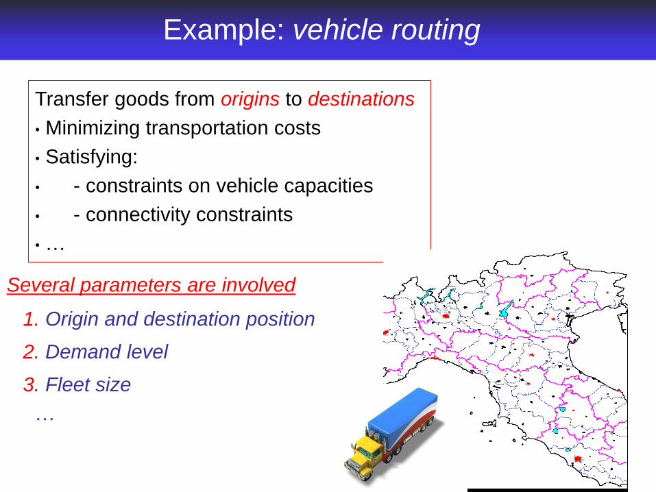
Example: vehicle routing

Transfer goods from origins to destinations

• Minimizing transportation costs

• Satisfying:

• - constraints on vehicle capacities

• - connectivity constraints

• …

Several parameters are involved

1. Origin and destination position

2. Demand level

3. Fleet size

…

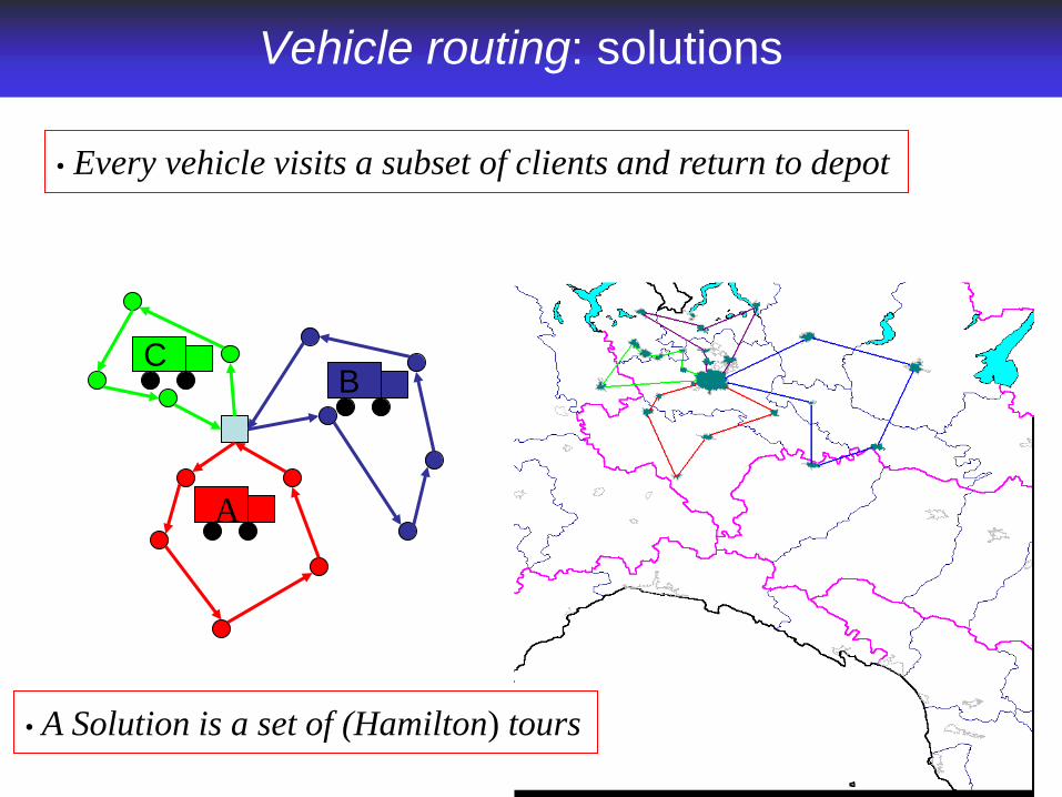
A

C B

• Every vehicle visits a subset of clients and return to depot

• A Solution is a set of (Hamilton) tours

Vehicle routing: solutions

A famous instance

Standard test instance G-n262-k25 (Gillett & Johnson 1976)

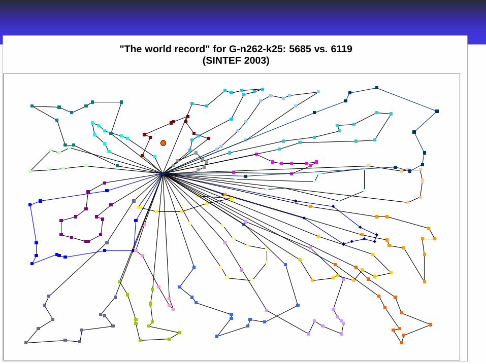
"The world record" for G-n262-k25: 5685 vs. 6119 (SINTEF 2003)

Inventory routing problem (IRP):

establish when and how much

produce and stock

Inventory level,

production

•Time •LB

•UB

Mixed problem: plan production and

transport of goods so as production is

never halted and warehouses are

never empty.

Lot sizing and rounting

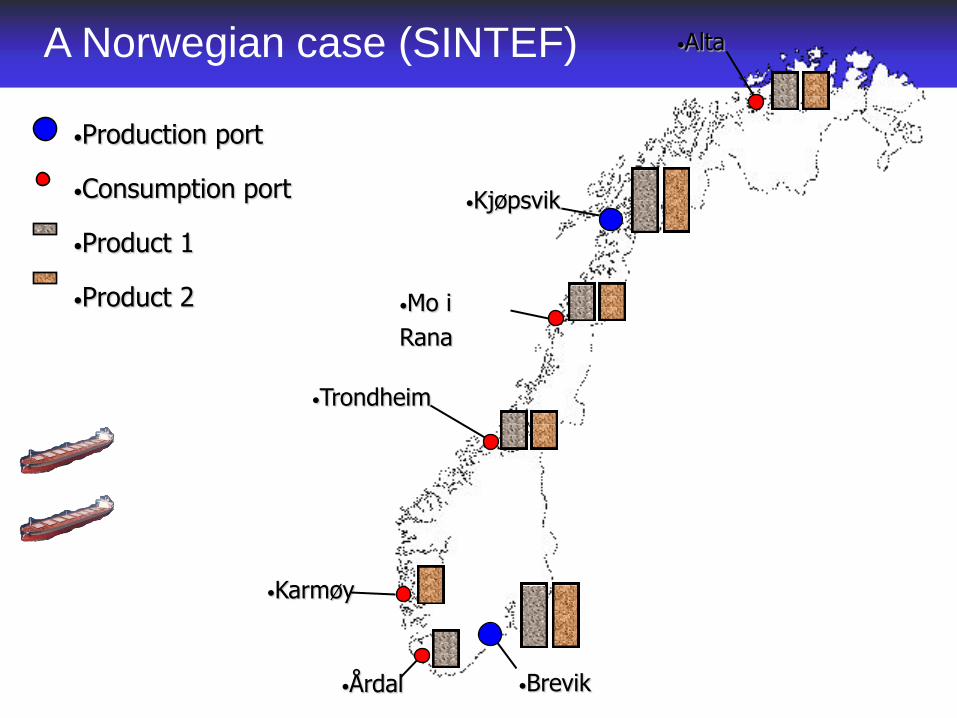
•Production port

•Consumption port

•Product 1

•Product 2

•Kjøpsvik

•Brevik

•Alta

•Mo i

Rana

•Trondheim

•Karmøy

•Årdal

A Norwegian case (SINTEF)

Mathematical Optimization Course

Basic combinatorial optimization problems: shortest path, minimum spanning tree, maximum flow, minimum cut.

Connections with linear programming and polyhedral theory: convexity, representation of polyhedra, formulations

Integer Polyhedra

Methods: heuristic algorithms

Methods: exact approaches

Outline of the course

LP-duality, basic relations

Dual Pair

Given a linear program (primal) (P)

min cTx

Ax b

x 0

(P)

A Rm×n, c Rn , b Rm x Rn

We associate a dual problem (D)

OBS a dual variable for each primal constraint, a dual constraint for each primal variable

y Rm

max bTy

ATy c

y 0

(D)

(P) can be infeasible, or unbounded, or the minimum is finite.

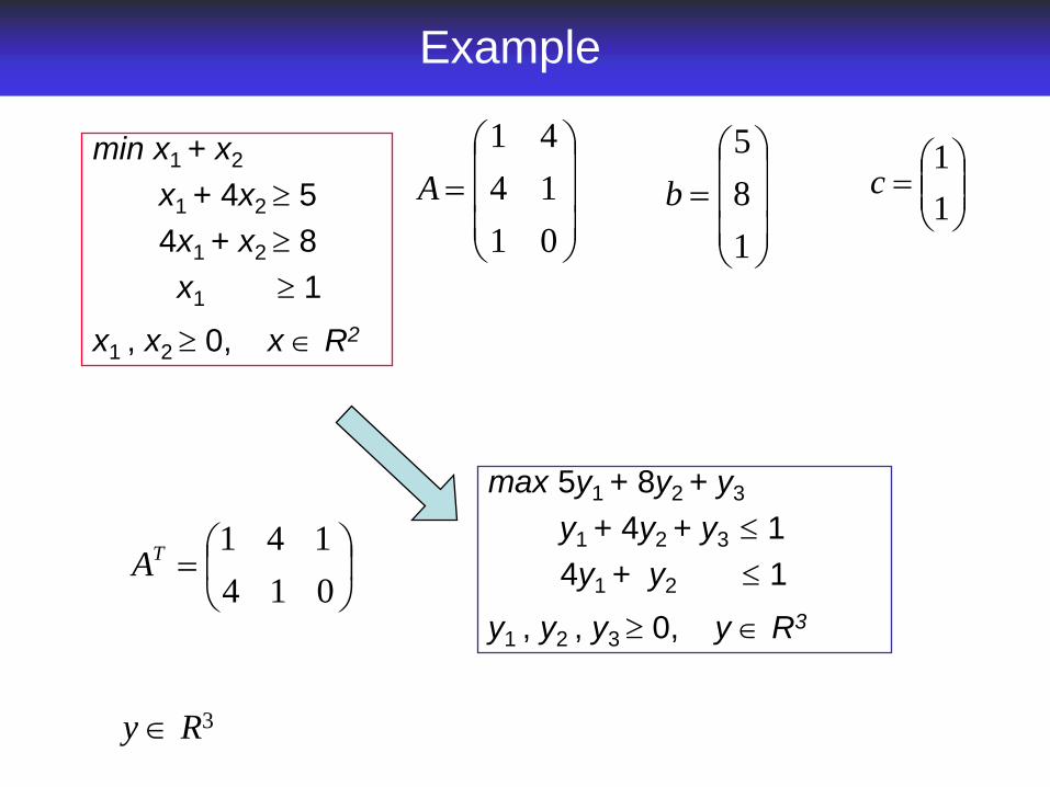
Example

y R3

0

1

4

1

4

1

A

1

1c

1

8

5

b

014

141TA

min x1 + x2

x1 + 4x2 5

4x1 + x2 8

x1 1

x1 , x2 0, x R2

max 5y1 + 8y2 + y3

y1 + 4y2 + y3 1

4y1 + y2 1

y1 , y2 , y3 0, y R3

General Form

PRIMAL DUAL

constraints

min max

bi

bi

= bi

0

constraints variables

variables 0

free

0

0

free

cj

cj

= cj

Dual variables correspond to primal constraints

Dual constraints correspond to primal variables

Exercise: Derive some of these rules from the canonical forms

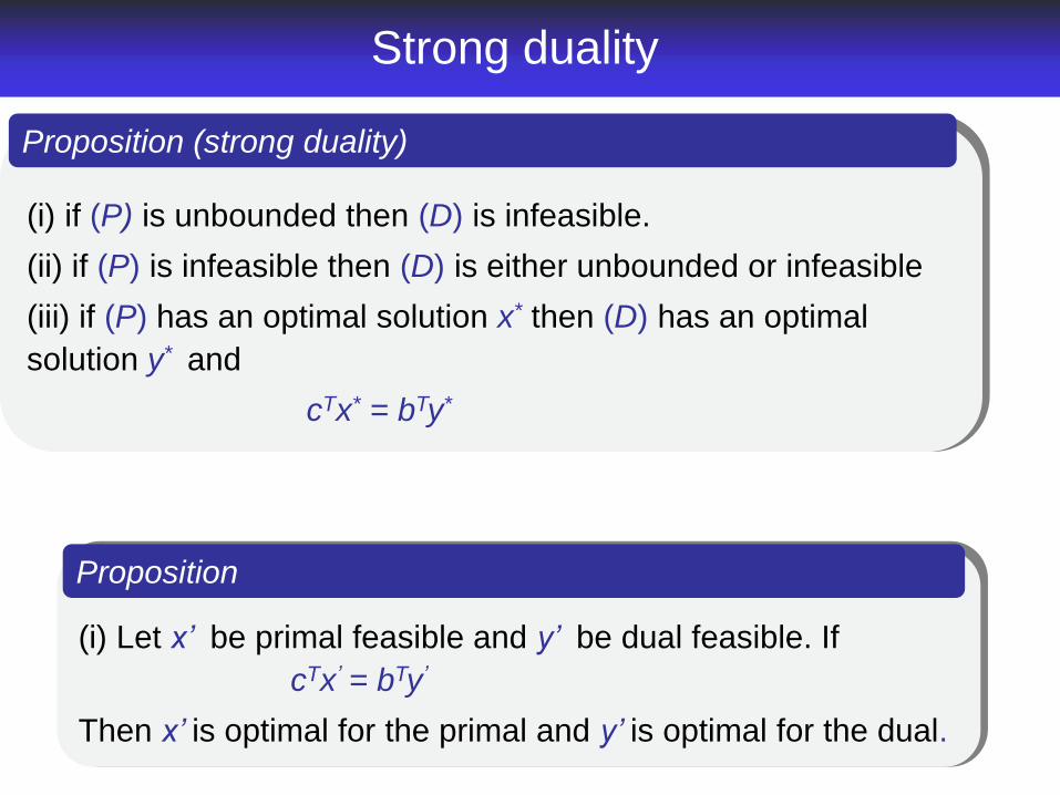
Strong duality

(i) if (P) is unbounded then (D) is infeasible.

(ii) if (P) is infeasible then (D) is either unbounded or infeasible

(iii) if (P) has an optimal solution x* then (D) has an optimal

solution y* and

cTx* = bTy*

Proposition (strong duality)

(i) Let x’ be primal feasible and y’ be dual feasible. If

cTx’ = bTy’

Then x’ is optimal for the primal and y’ is optimal for the dual.

Proposition

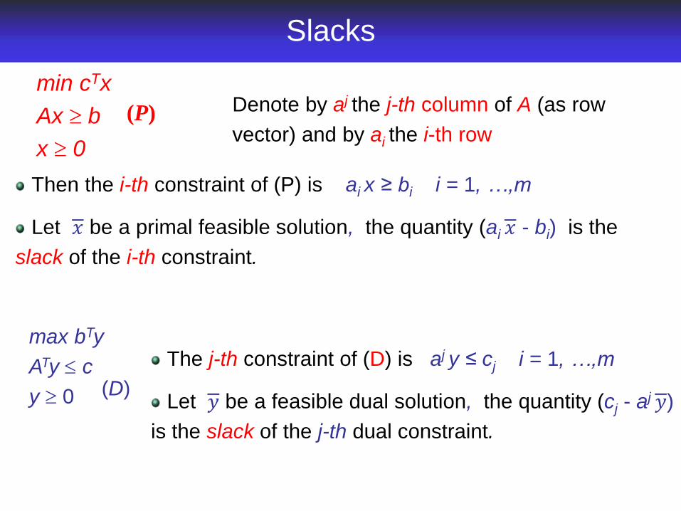
Slacks

Denote by aj the j-th column of A (as row

vector) and by ai the i-th row

min cTx

Ax b

x 0

max bTy

ATy c

y 0

Then the i-th constraint of (P) is ai x ≥ bi i = 1, …,m

Let 𝑥 be a primal feasible solution, the quantity (ai 𝑥 - bi) is the

slack of the i-th constraint.

The j-th constraint of (D) is aj y ≤ cj i = 1, …,m

Let 𝑦 be a feasible dual solution, the quantity (cj - aj 𝑦)

is the slack of the j-th dual constraint.

(D)

(P)

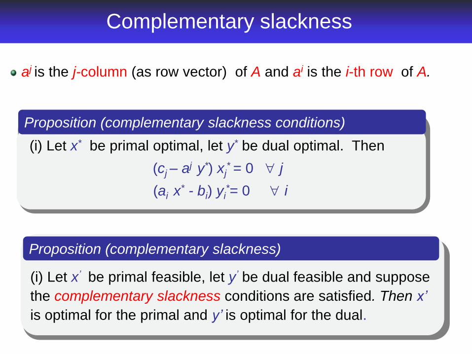
Complementary slackness

(i) Let x* be primal optimal, let y* be dual optimal. Then

(cj – aj y

*) xj* = 0 j

(ai x* - bi) yi

*= 0 i

Proposition (complementary slackness conditions)

aj is the j-column (as row vector) of A and ai is the i-th row of A.

(i) Let x’ be primal feasible, let y’ be dual feasible and suppose

the complementary slackness conditions are satisfied. Then x’

is optimal for the primal and y’ is optimal for the dual.

Proposition (complementary slackness)

Exercise

Model this problem as a linear program (example taken from

Bradley, Hax, Magnanti, Applied Mathematical Programming)