A Human Capital Model of the Effects of Abilities

and Family Background on Optimal Schooling

Levels

Tracy L. Regan∗, Ronald L. Oaxaca†, and Galen Burghardt‡

May 1, 2003

Abstract

This paper develops a theoretical model of earnings where human capital is

the central explanatory variable. The analysis and estimation strategy stems

from the Mincerian (1974) simple schooling model. We incorporate human cap-

ital investments (i.e., schooling) into a model based on individual wealth maxi-

mization. From this model we can derive and utilize the conventional economic

models of supply and demand. We use data collected from the NLSY79 to strat-

ify our sample into one-year work-experience intervals for the years 1985-1989

to identify the “overtaking” cohort (i.e., the years of work experience at which

an individual’s observed earnings approximately equal what they would have

∗Department of Economics, The University of Arizona, McClelland Hall #401, P.O. Box 210108,

Tucson, AZ 85721-0108. Comments/inquiries can be directed to tregan@u.arizona.edu, [W] (520)

621-6224, [F] (520) 621-8450.†Department of Economics, The University of Arizona, McClelland Hall #401, P.O. Box 210108,

Tucson, AZ 85721-0108.‡Carr Futures Inc., 150 S. Wacker Dr., Suite 1500, Chicago, IL, 60606.

1

been based on his schooling and ability alone). We find that the “overtak-

ing” year of work-experience occurs for individuals who have 13 “FTE” years

of work-experience, which is associated with an average 9.7 percent rate of re-

turn to the average optimal 11.4 years of schooling. Ultimately, we estimate

an earnings transformation (production) function, a derived internal rate of re-

turn (demand) function, and a discounting rate of interest (supply) function to

derive a reduced-form optimal level of schooling function for this “overtaking”

cohort. Our estimation strategy employs the AFQT score as an ability proxy

and also considers the possible endogenous nature of this variable (which we

ultimately reject). This paper explores several estimation strategies including

OLS, 2SLS, and NLSUR/NLOLS.

Acknowledgement 1 We would like to thank the workshop participants at the

University of Arizona for their helpful comments and insights. Special thanks

to Price Fishback and Alfonso Flores-Lagunes. We also appreciate the research

assitance provided by Laura Martinez.

2

I. INTRODUCTION

Becker’s 1962 paper defines human capital investments to be any “activities that

influence future real income through the imbedding of resources in people.” (Becker,

1962, pp. 9) Human capital investments are of wide ranging interest because they can

be used to explain income disparities across people, over space, and over time. Labor

earnings are typically people’s primary source of income. Human capital investments

include schooling, on-the-job-training (OJT), routine medical exams, healthy diets,

etc.-in other words, anything that can help increase worker productivity. Schooling is

a unique type of investment in that it affects not only current day consumption but

also future earnings potential as well. Individuals choose to invest in schooling until

their marginal rate of return equals their discounting rate of interest. More practically

speaking, they operate in such a way so as to maximize their expected (discounted)

future earnings stream. Social and intellectual interest in income disparities, primar-

ily stemming from differing schooling levels, has generated an enormous amount of

attention across disciplines. There is a vast literature supporting/reflecting such an

interest.

This paper specifies and estimates a human capital model that is based on indi-

vidual wealth maximization. We use an earnings-schooling relationship to calculate

individual marginal rates of return to schooling and discounting rates of interest.

From these we can identify and estimate supply and demand functions for schooling-

investment. We ultimately arrive at an optimal level of schooling equation that

accounts for permanent family income levels, family size, and abilities. We consider

two different proxies for ability, but ultimately confine our attention to just one. We

consider the possible endogeneity of this variable as well. Our estimation strategy

involves disaggregating our sample into one-year work-experience intervals for 1985-

1989. We then estimate a log wage equation to identify the work-experience cohort

3

which minimizes the estimated residual standard error and three other model selec-

tion criteria, namely the Akaike information criterion, the Schwarz criterion, and the

Amemiya’s prediction criterion. Once we have identified this group we proceed with

the rest of our estimation. We employ the following estimation strategies in this

paper: OLS, NLSUR/NLOLS, and 2SLS.

This paper is organized as follows: Section II provides the background and literature

review. Section III discusses the conceptual framework that underlies the analysis.

Section IV discusses the data used in the analysis. Section V presents the results and

Section VI discusses them and provides alternative estimation strategies. Finally,

Section VII concludes. A bibliography, appendices, and supporting tables and figures

are provided at the paper’s end. The Technical Appendix is available upon request

from the authors.

II. Background and Literature Review

A tremendous amount of the economics literature has been devoted to studying

human capital investments and the economic rates of return, particularly to education.

Researchers have exploited the models and theories developed by Mincer and Becker

in their attempts at getting purer, more accurate, and more sophisticated rates of

return. Various econometric strategies have been developed and utilized to account

for the potential measurement error, omitted variables bias, and selection bias of the

traditional log wage model.

Becker’s 1962 paper is one of the seminal works done on human capital invest-

ments. Becker provides the justification for an age-earnings profile that is both steep

and concave. Its shape stems from the fact that such human capital investments

lower observed earnings at young ages because any such costs are deducted from an

individual’s wage. However, observed earnings rise in later years because the returns

to such investments are then added on to an individual’s wage. Several years later

4

Willis and Rosen (1979) published a paper where they attempt to estimate lifetime

earnings conditional on actual school choices (i.e., high school or college) that were

purged of any selection bias. They estimate a structural probit for data collected from

the NBER-Thorndike-Hagen survey of 1968 (i.e., male WWII veterans). Willis and

Rosen do find that there is positive selection bias in observed earnings and estimate

rates of return to be about 9 percent.

Some of the more recent studies on human capital investments and the associated

rates of return to school have delved deeper into such econometric issues and also

presented modifications to the standard Mincerian approach of explaining earnings.

In 1983, Behrman and Birdsall extend the simple log wage model to incorporate not

only school quantity but quality as well, as proxied by the years of schooling completed

by a pupil’s teacher. They argue that the omission of quality biases the traditional

OLS estimates upwards. Behrman and Birdsall’s analysis uses data collected from

the 1970 Brazilian Census. Card and Krueger (1992) use an approach similar to

Behrman and Birdsall in estimating the effects of school quality on rates of return to

education. They proxy for school quality with various measures (e.g., pupil/teacher

ratio, average teacher term length, relative teacher pay) found in the Biennial Survey

of Education. Using the 1980 Census, Card and Krueger estimate earnings functions

for white men born between 1920 and 1949. They find that men educated in states

with higher quality schools, better-educated teachers, and a higher fraction of female

teachers have higher rates of return to each additional year of schooling.

Another modification to the log earnings function comes from the work done by

Altonji and Dunn in 1996. They incorporate parental education levels into their

model by interacting them with their children’s education levels. Using a fixed-effects

estimation strategy, on data collected from the NLSY66 and PSID68, they find mixed

evidence on the role of parental education in the human capital function. Ashenfelter

and Zimmerman (1997) continue to investigate the effects of family background on the

5

economic rates of return to education. Using data collected from the NLSY66, they

gather information on father-son and sibling (i.e., brother-brother) pairings. They

incorporate a family-specific fixed effect into the standard Mincerian log earnings

function and ultimately arrive at a correlated random effects model. Ultimately,

Ashenfelter and Zimmerman use a seemingly unrelated regressions approach and find

an upward bias in the estimated rates of return from omitted variables. This bias

is offset by a downward bias due to measurement error in self-reported schooling

levels. Hence, controlling for omitted variables and measurement error yields results

comparable to the conventional rates of return obtained from OLS.

Family background again comes to the forefront in Lang and Ruud’s (1986) work.

The approach taken by Lang and Ruud is similar to ours but differs on several im-

portant points. Like us, Lang and Ruud employ data collected from the NLSY (the

1966 wave instead) but they use potential, rather than actual work experience. They

consider single, rather restrictive measures of socioeconomic status (i.e., the Duncan

Index) and ability (i.e., IQ). Furthermore, their wage regressions employ an individ-

ual’s hourly wage as the dependent variable which glosses over the well-known fact

that individuals who have a higher hourly wage tend to work more because of their

high opportunity costs to leisure. In spite of the paper’s shortcomings they do find

that their measures of individual discount rates, implicit in the education investment

decision, do not vary with socioeconomic background. Family background does how-

ever help to explain differences in individual levels of education, primarily due to

variation in their attainment speeds.

Ability measures have always received much attention in the human capital liter-

ature. Such unobservables have often posed problems for researchers. Researchers

have most often proxied ability measures with IQ scores, or other such similar tests.

However, in 1994, Ashenfelter and Krueger compile a unique data set consisting of

twins (mostly identical) to address such issues. Using an instrumental variables tech-

6

nique, they do find significant evidence of measurement error that biases the rates of

return down. When they adjust for such measurement error they find rates of return

between 12 and 16 percent, much higher than the conventional estimates. Moreover,

they conclude that any unobserved ability (i.e., omitted variables) does not bias the

rates of return upwards.

Several of these different econometric estimation strategies are surveyed and sum-

marized in Card’s 1994 work. The studies he cites either use a fixed effects or instru-

mental variables method in accounting for the causal effect of schooling in the labor

market. All but one of these studies find that the OLS estimates to rates of return

are biased down (by about 10 to 30 percent). While many of these studies can be

criticized for their identification strategy, imprecision, strict underlying assumptions,

and unique samples, their similar findings do warrant careful rethinking.

III. CONCEPTUAL FRAMEWORK

Throughout this paper we will treat the schooling decision as an investment activity

and focus solely on it. First, we posit the existence of an earnings transformation

function1 ,2 and define it as follows,

Y = F (S,A). (1)

This function relates an individual’s annual earnings, Y , to his/her years of schooling,

S, and to his/her natural ability, A. For our earnings function to exhibit the conven-

1Burghardt and Oaxaca (1979) state that, “As Rosen (1973) points out, the transformation

function is derived from a production function of knowledge whose arguments are schooling and

ability. The units of knowledge (human capital) are multiplied by a constant market rental rate

on human capital to yield earnings. The production function itself is derived from a learning

function that governs the rate at which knowledge can be produced from prior schooling and ability.”

(Burghardt and Oaxaca, 1979, pp. 3)2Lazear (1977) frames his discussion of education in the context of a production function.

7

tional positive, but diminishing marginal returns to schooling and positive returns to

ability, we need the following inequalities to be satisfied,

FS, FA > 0 and FSS < 0. (2)

We might also expect more able people to reap greater rewards (i.e., in the form of

their resulting wage structure) to increased schooling levels and vice-versa as well3.

Thus,

FSA = FAS > 0. (3)

In the analysis that follows it is more convenient to think of our earnings transfor-

mation function in its log form,

lnY = lnF (S,A). (4)

Now, it is much easier to interpret and derive the marginal rate of return to schooling.

Let us define the marginal rate of return to schooling, r, as follows,

r =∂ lnF (S,A)

∂S. (5)

In order for the marginal rate of return to schooling to increase with ability (and

hence for the demand for schooling to increase with ability) we need the following

inequality to be maintained4,

FFSA > FAFS. (6)

3For a general, perhaps dated, discussion of the effects of schooling and ability (and their inter-

action) on log earnings, see Hause (1972).4The proof of this inequality is found in Appendix 1.

8

Next, we will assume that all relevant costs are just foregone earnings and that an

individual seeks to maximize the present value, of his/her lifetime earnings over an

infinite horizon5 subject to the constraint imposed by (1). Formally speaking, we can

mathematically represent an individual’s maximization problem as,

MaxVS

=

Z ∞

S

Y e−itdt subject to Y = F (S,A), (7)

where V is the present value of lifetime earnings, i is a fixed discounting rate of

interest, and t is the index of integration.

We can then simplify the present value of lifetime earnings and take the log of the

resulting expression to obtain,

lnV = lnY − iS − ln i. (8)

Taking derivatives with respect to S we arrive at the following first order condition,

r = i. (9)

Hence, the optimal level of schooling for an individual occurs at the point where

his/her marginal rate of return to schooling exactly equals his/her discounting rate

of interest.

We can now put the above analysis into a conventional supply and demand frame-

work. We obtain an individual’s demand for investment in schooling by taking the

derivative of the log transformation function as defined in (4) with respect to school-

ing6. Hence, the demand for schooling can be expressed as,

r = r(S,A), (10)

5This infinite horizon is imposed for mathematical simplicity. An infinite horizon model has

been used by numerous other researchers as well. See Lang and Ruud (1986).6For a given individual, his/her abiliity level is assumed to be fixed.

9

or equivalently as,

Sd = Sd(i, A),

where Sd is the level of schooling demanded at each discounting rate of interest for

an individual with a given ability level A7. Thus, we allow the demand for schooling

to be the marginal rate of return.

We can derive an individual’s supply function for school investment from the present

value function as defined in (8). Simple manipulation of this expression yields,

lnY = ln(iV ) + iS. (11)

Differentiating this expression with respect to S yields an individual’s supply curve.

This establishes the relationship between the supply of schooling and the discounting

rate of interest. It should be noted that an individual’s discounting rate of interest,

i, is uniquely fixed and does not vary with the level of schooling. However, since

i can also be interpreted as the marginal opportunity cost of an additional year of

school, it is reasonable to assume that i can vary across individuals. For example,

we would probably expect the discounting rate of interest to be higher for children

from poorer families than that of children from wealthier families. The same could

be said of children from larger families as compared to children from smaller families.

Hence, we can define i as a function of an individual’s family characteristics,

i = i(X), (12)

7The derivation of this equivalent expression is most clearly seen when we consider the stochastic

estimation to equation (4) (i.e., equation (15)). Taking the derivative of the lnY with respect to

S yields the marginal rate of return. Rearraning this expression and solving for S yields a level of

schooling that is a function of r and A. Imposing the equilibrium condition that r = i makes the

demand for school a function of i and A.

10

whereX denotes a vector of family background variables. In our analysis these include

family size and permanent family income levels.

Combining (9), (10), and (12) we can simply define the optimal level of schooling

as,

S∗ = f(X,A). (13)

We can graphically illustrate this optimal level of schooling using both a supply and

demand framework and a framework relating the log earnings functions8. This can

be seen in Figure 1. The top graph relates the log earnings transformation function

to the log earnings present value functions as defined in (11). The log earnings

transformation function is a concave curve reflecting the positive, but diminishing

marginal returns to schooling. The log earnings present value functions are a series

of straight lines relating lnY and S at a given discounting rate of interest, i. The

optimal level of schooling, S∗, occurs at the point of tangency between these two

curves-the point at which discounted lifetime earnings are maximized. The bottom

graph tells the same story, just from a different viewpoint. This framework relates the

downward sloping demand function, as defined in (10), to the infinitely elastic supply

curve, as defined in (12). The intersection point between these two curves corresponds

to the point where the discounting rate of interest exactly equals the marginal returns

to schooling (i.e., the equilibrium as defined in (9)). This in turn establishes again,

the optimal level of schooling, S∗. These two frameworks graphically establish the

solution to the maximization problem as defined in (7).

We can now consider the situation in which ability levels and discounting rates of

interest are allowed to vary across individuals. Figure 2 depicts this situation. Again

in the top framework we see individuals’ optimal schooling levels being established

8Becker and Chiswick (1966) give a very general discussion of how human capital investment can

be nested in the context of a supply and demand curve analysis.

11

by the point of tangency between their log earnings transformation functions and

their log earnings present value functions. The bottom framework achieves the same

results, by utilizing the individual-specific supply and demand intersections instead.

Hence, fitting a line through the set of tangency points in the top graph parallels the

development of Mincer’s simple schooling model9 which is,

lnYj = β0 + β1Sj + uj, (14)

for individual j.

Next, we will discuss the empirical specification that underlies the econometric

analysis. The stochastic approximation10 to the transformation function as defined

in (4) is,

lnYj = β0 + β1Sj + β2AjSj + β3S2j + u1j, (15)

where j denotes the individual and u1j11 is an error term. To maintain the relationship

as defined in (4), we would expect the following signs on the coefficients:

β1,β2 > 0 and β3 < 0. (16)

The schooling-investment demand function is obtained by differentiating (15) with

respect to S. Thus, obtaining,

rj = β1 + β2Aj + 2β3Sj , (17)

9Burghardt and Oaxaca (1979) address the identification of this model. Since the model is not

identified, β1, has no economic meaning. However, its interpretation as an average rate of return to

schooling is maintained throughout the analysis.10See Heckman and Polachek (1974) for a discussion of the appropriateness of this functional form.11We assume u1j ∼ iidN(0,σ21). The Bera and Jarque (1981, 1982) test confirms this assumption.

The details of this test can be found in Appendix 2.

12

where rj =∂ lnYj∂Sj

. We specify the schooling-investment supply function to be a linear

function of various family background variables. Consider the following specification,

ij = θ0+θ1Sfj+θ2Smj+θ3(Sfj+Smj)+θ4DV Sfj+θ5DV Smj+θ6Nj+θ7Nj+u2j, (18)

where Sfj is the schooling level of an individual’s father, Smj is the schooling level

of an individual’s mother, Nj is the family size, and u2j12 is an error term. In

the above construct, we have proxied permanent family income with the schooling

levels of an individual’s parents13. So as to not lose observations, and to maintain

a constant sample size across regressions14, we imposed an education level of zero

years for any respondent’s parent whose education level was reported as a missing

value. We then constructed dummies indicating whether or not we imposed such a

value. Hence, DV Sf takes on a value of “1” if we replaced a missing value for the

respondent’s father’s education level with a zero. Similar reasoning applies for the

dummy variable on a respondent’s mother’s schooling level, DV Sm15.

The above construct allows for a nice interpretation of the coefficients. The θ1 and

θ2 capture the pure wealth effects of family income on an individual’s discounting

rate of interest. Hence, we would expect these two parameters to have negative

signs because an individual’s discounting rate of interest (or alternatively, his/her

12We assume u2j ∼ iidN(0,σ22).13We considered several other proxies of permanent family income, namely the Duncan Socioeco-

nomic Index and variations of the parental schooling levels—the average level, the maximum level,

and the head of the household’s level. We abandoned such alternatives because we either lost too

many observations or because we feared the bias that would result from a subjective judgement of

the importance of parental schooling.14The importance of maintaing a constant sample size across (15), (19), and (22) will become

evident in the NLSUR estimations that follow.15Of the 239 observations, only 26 (22) respondents did not report their father’s (mother’s) school-

ing level.

13

marginal opportunity cost of an additional year of schooling ) decreases with his/her

family wealth (i.e., the individual is more patient and can postpone earnings for

more schooling). The θ3 however captures the effect of family wealth on potential

financial aid. Since financial aid offices base their decisions purely on family wealth,

not individual parental contributions, we sum these two variables together and expect

their common parameter, θ3, to have a positive sign. Hence, children from richer

families have less of a chance of receiving financial aid which in turn increases their

discounting rate of interest. We can decompose the effects of family size on an

individual’s marginal opportunity cost of an additional year of schooling into two

separate effects. The θ6 parameter captures the pure income effect of family size.

We would expect individuals from larger families to have increased opportunity costs

to additional schooling, hence θ6 should be positive. However, the larger a family, the

more widely the (financial) resources are spread and hence the greater the opportunity

for financial aid assistance. Thus, we would expect θ7 to be negative.

Since the coefficients are not identified in the above specification, we collect terms

and arrive at the following functional form,

ij = α0 + α1Sfj + α2Smj + α3DV Sfj + α4DV Smj + α5Nj + u2j, (19)

where,

θ1 + θ3 = α1, (20)

θ2 + θ3 = α2,

and

θ6 + θ7 = α5.

Hence, the above specification identifies the relative parental contributions on wealth

14

effects, aside from the financial aid effects16. We can determine which of the effects

are larger by noting the sign of the estimated coefficient.

The reduced-form optimal level of schooling equation is obtained by substituting

(17) and (19) into the individual-specific equilibrium condition,

rj = ij. (21)

When we do this and solve for S∗, we obtain,

S∗j = γ0 + γ1Sfj + γ2Smj + γ3DV Sfj + γ4DV Smj + γ5Nj + γ6Aj + u3j, (22)

where

γ0 =α0 − β12β3

, (23)

γ1 =α12β3

,

γ2 =α22β3

,

γ3 =α32β3

,

γ4 =α42β3

,

γ5 =α52β3

,

γ6 =−β22β3

,

u3j =u2j2β3

,

and

σ23 =σ224β23

.

The signs on the coefficients establish the net effect of the direct and indirect (i.e.,

through financial aid awards) wealth effects on schooling. The only coefficient that

16Specifically, this is because α1 − α2 = θ1 − θ2.

15

we could sign at this point would be that of ability. It is reasonable to expect that

more able people would reap greater rewards from increased schooling levels. Thus,

we expect γ6 to be positive.

Due to the fact that an individual’s discounting rate of interest and marginal rate

of return to schooling are not observable, we must estimate them in order to identify

the supply and demand functions. Hence, in estimating the marginal rate of return

to schooling, we use the estimated parameters obtained from the OLS estimation of

(15). This then establishes an estimated marginal rate of return to schooling, rj, for

each individual. We then impose the equilibrium condition as defined in (21) to get

an estimated discounting rate of interest, ıj. In other words, rj = ıj. We use these

estimated marginal rates of return and discounting rates of interest as the dependent

variables in the demand of and supply for schooling investment functions, respectively.

The estimation strategy used here follows a procedure Mincer (1974) used when

estimating the simple schooling model of equation (14). In this work he seeks to “gain

understanding of the observed distribution and structures of earnings from informa-

tion on the distribution of accumulated net investments in human capital among

workers.” (Mincer, 1974, pp. 2) He considers a theoretical model of earnings where

human capital is the central explanatory variable. Mincer argues that experience,

more than age, explains earnings differentials due to education. He argues that the

correlation between log earnings and education is strongest in the first decade of work

experience. Mincer introduces the notion of an “overtaking” year in which an indi-

vidual’s observed earnings are most reflective of his/her investment in school (and

innate ability). At this particular point in time the distortion from post-schooling in-

vestments (i.e., OJT) is minimized and the return on an individual’s prior investment

(i.e., schooling) equals the cost of the current investment (i.e., OJT). An individual’s

earnings at this “overtaking” year provide the best test of the simple schooling model.

This “overtaking” year is usually eight years after an individual has left school when

16

an individual has between seven and nine “years” of work experience.

Goodness of Fit Measures

In our attempts to identify the “overtaking” year of work-experience, we considered

five separate “goodness of fit” measures for the model as described in (15)17. The

most typical and singular way of gauging the “goodness of fit” of a regression is the

use of the R2 measure. The R2 measures the proportion of the total variance in

the dependent variable that is explained by the model (linearly). Thus, we seek

to maximize the R2. This measure has been criticized for its obvious fault—it can

be inflated just by including more regressors. Theil (1961) purported the use of an

adjusted R2 measure, R2, that corrects for the degrees of freedom. We chose not to

include the adjusted R2 measure because the number of regressors in (15) does not

vary.

It is the belief of some that even the R2does not impose a harsh enough penalty for

the loss in degrees of freedom. Hence, the next three measures we consider attempt

to correct this problem. All three of these selection criterion seek to minimize the

mean-squared error (MSE) of prediction (as opposed to the residual standard error),

E(lnYf −dlnY f)2, (24)

where lnYf is the future value of lnY and ln bYf is the predicted future value.The first of these selection criteria is Amemiya’s (1980) prediction criteria (PC).

We seek to minimize the following,

PC =SSE(1 + k

N)

N − k = σ21(1 +k

N), (25)

17All of these “goodness of fit” measures are based on the fact that we have a reasonably large

sample (i.e., greater than 100 observations). This however is not really much of a concern for the

earlier cohorts.

17

where SSE denotes the total sum of squared errors, k is the number of regressors

(inclusive of the constant term), N refers to the sample size, and σ21 is the error

variance of u1.

Another more general selection criterion is the use of Akaike’s (1973, 1974) infor-

mation criterion (AIC). It seeks to minimize,

AIC = lnSSE

N+2k

N≈ lnσ21 +

2k

N. (26)

The third selection criterion was developed by Schwarz (1978). The Schwarz criterion

seeks to minimize,

SC = lnSSE

N+k lnN

N≈ lnσ21 +

k lnN

N. (27)

It should be noted that the three criterion discussed above are typically nested

in discussions of regressor selection18. Typically researchers are testing different

models using the same data set. We however, are testing a common model using

different samples of our data to determine which work-experience cohort best suit its

predictions.

The last “goodness of fit” measure we consider is simply the estimated standard

error of the regression. We seek to minimize the estimated residual variance,

bσ21 = SSEj(N − k) , (28)

(or alternatively its square root which is the estimated residual standard error). The

estimated residual variance helps to explain all the variance in the model that has

not been explained by the regressors. Thus, the smaller it is the more explanatory

18For nice discussions of these selection criterion see Greene (1997), Kennedy (1998), Maddala

(2001), and Judge et al. (1988).

18

power we can attribute to our model.

IV. DATA

The data used in this paper is from the National Longitudinal Survey of Youth

1979 (NLSY79). The NLSY79 consists of 12,686 young men and women, living in

the U.S., who were between the ages of 14 and 22 years when the first survey was

conducted in 197919. In 1998, the most recent wave of the survey, 8,399 civilian and

military respondents were interviewed from the 9,964 eligible persons, hence yielding

an overall retention rate of 84.3 percent.

The demographic variables for each respondent were collected from the 1979 inter-

view. We confined our attention to include only white males. The resulting sample

size is 4,393 persons. From this 1979 interview we were able to get several measures

of a respondent’s family background/income level. These measures include the re-

spondent’s family size and the highest grade completed by a respondent’s mother and

father. The NLSY79 provides three different measures used to gauge a respondent’s

ability. The first of these, which we chose not to use because of the small number

of respondents, is the total Intelligence Quotient (IQ) score. The second of these

is the Knowledge of the World of Work (KWW). The third is the Armed Forces

Qualification Test (AFQT).

The educational attainment and enrollment status was available for each survey

year. We have measures indicating both the highest grade completed by a respondent

and his current enrollment status. When performing the econometric analysis, we do

not include any respondent who is currently enrolled in school for that year because

such individuals have not fully realized the gains to school in terms of their resulting

wage structure yet. We also omit anyone who attended school after 1989 to ensure

19There is oversampling of the poor and people in the military.

19

that the wages we observe are truly reflective of final20 schooling choices21.

The income variables were collected from the main NLSY79 files as well. The

dependent variable in the log earnings regression is the log of a respondent’s total

income from wages and salary in the respective year. Using the Consumer Price

Index (CPI) for all urban consumers, as published by the BLS (Bureau of Labor

Statistics), we deflated the income figures and express them in terms of 1985 dollars.

In our analysis, we consider only people who earned at least $500 in nominal terms

for a given year.

The variables used in the construction of the experience measures were collected

from the supplementary NLSY79 work history file. Since each respondent is assigned

a unique identification code, we were able to merge the two data sets. Due to this

detailed collection of work experience variables, we do not have to use less accurate,

potential work experience measures. A respondent’s work experience for a given year

is calculated by summing the hours worked in that year and all prior years (since

1979) and then dividing through by 2080. Taking account of the fact that many of

our respondents were older than 18 years (the usual age that one graduates from high

school in the U.S.) and had potentially been working for several years prior to the

first survey in 1979, we constructed a variable to measure their experience prior to

1979. This variable is calculated as follows,

20The term “final schooling” is used somewhat loosely here because we can only observe individual

schooling choices/enrollment through 1998, the most recent wave of the NLSY79 survey that we have.

21Including such individuals yields estimates of (15), (19), and (22) that are marginally more

significant. By focusing on those individuals who have finished their educational investment through

1998, we only lose nine observations for the 13 year work-experience cohort. The earlier cohorts

considered, the more observations lost. The figures in Table 4 do however support the choice of the

13 year work-experience cohort as the “overtaking” cohort.

20

Experience prior to 1979 = (Age1979−Schooling1979−6)∗(Work Experience1979/2080).(29)

Hence, this gives us a measure of “full-time equivalent” (FTE) work experience22.

FollowingMincer’s lead, we stratified our sample into one-year FTEwork-experience

intervals for the years 1985-198923. Ultimately this procedure controls for experience

without making it explicit in any of the equations. (15) is then estimated separately

for each work-experience cohort. Running each regression separately allows for full

interaction effects of work experience on each coefficient. The earnings data in the

model as defined by (15), (17), (19), and (22) reflects not only ability and schooling-

investment decisions but post-schooling investments (e.g., work experience, on-the-

22It should be noted that most often these “years” of work-experience do not coincide calendar

years.23We chose to confine our attention to the years 1985-1989 for several reasons. First, as previously

stated, Mincer argues that the correlation between log earnings and education is strongest in the

first decade of work experience. The NLSY79 began in 1979 and the latest year we chose to look at

was 10 years later, in 1989. Second, Mincer finds that the “overtaking” year occurs eight years after

an individual has left school and has acquired seven to nine “years” of work experience. In the first

year of the survey, our respondents are between 14 and 22 years old. Roughly, half are under 18

years and it is reasonable to assume still enrolled in school. Using 1985 as a lower bound allows our

youngest respondents to probably have acquired at least four years of work experience. We also do

not, at this point, consider earlier years, like 1980 for instance, because the closer to the first survey

year the cruder our approximations are of the respondents’ true work experience. This is due to the

fact that we had to estimate their work experience prior to 1979. Going as late into the survey as

1989 probably biases us towards finding a later “overtaking” year if anything. Furthermore, as a

rough rule of thumb you can estimate the rate of return to education as the inverse of the overtaking

cohort. Roughly speaking, in 1985, six calendar years have passed since the first survey year and

we would calculate a 16.7 percent rate of return to schooling. This figure seems a bit high, but for

1989 we would get a 9.1 percent rate of return which seems more reasonable and is similar to rates

previously found by other researchers.

21

job training) as well. Thus, ignoring the potential correlation between schooling and

work-experience in cross-sections would bias the OLS estimates. By stratifying our

sample into work-experience cohorts we purge the model of any post-schooling in-

vestment decisions. Thus, there exists an “overtaking” year in which an individual’s

earnings are most reflective of his/her natural ability and schooling levels alone. We

reasonably assume that this “overtaking” year varies across individuals, even within

a given work-experience cohort. Thus, we stratify our sample into one-year work-

experience intervals for 1985-1989 so we can best identify the group whose earnings

are “free” of OJT effects.

V. Estimation and Results

As mentioned above, our statistical estimation concerns white males who earned

at least $500, in nominal terms, for a given survey year and who were not currently

enrolled in school or anytime after 1989. Table 1 provides the descriptive statistics

for each variable used in the analysis. The mean, standard deviation, maximum

value, minimum value, and the number of cases are given for the overall sample. On

average, our respondents are about 18 years old and seem to have the equivalent of a

high school education while their parent(s) appear to have completed through their

junior year of high school. On average, the respondents come from households with

three other members. The ability measures indicate average intelligence levels. From

these tables we can observe an upward trend in schooling levels, years of experience24,

24At first glance the maximum values for the years of work experience may look quite peculiar.

However, due to the construction of this variable it is quite possible for people to work the equivalent

of several years within a given calendar year. This is the case for multiple-job holders and over-time

workers. The maximum hours reported for any calendar year between 1979 and 1989 is 4992 (which

corresponds to 57 percent of total annual hours and 2.4 FTE years). The reporting of such large

values is relatively infrequent and the corresponding work-experience cohorts are rarely, if at all,

used in the following analysis. The work-experience frequency distributions in Table 2 support this

22

and wages over time.

Table 2 provides the frequency distributions for the work-experience cohorts in

1985-1989. As would be expected, the cohort encompassing the largest percentage

of respondents increases each year. However, as we move further in time we see a

greater dispersion of respondents into each of the cohorts. In 1985, 14.7 percent of the

sample had the modal experience that was about two years and in 1989, 9.3 percent

of the sample had the modal experience of seven years.

Sample Stratification

As was previously mentioned, we chose to stratify our sample into one-year full-

time equivalent intervals of work-experience for 1985-1989. Table 3 lists the number

of people in each respective cohort and the corresponding percentage they comprise

of the entire sample. The information contained in Table(s) 3 (and 4) correspond

to cohorts in which the sample size was reasonable, i.e., above 100. The proce-

dure for constructing the FTE work-experience intervals worked as follows: For

example, in constructing the one-year work-experience cohort, we included individ-

uals who reported having between one (inclusive) and two (not inclusive) years of

work-experience at any time between 1985 and 1989. Obviously, in using such a

decision rule we encountered the possibility of individuals who reported say, 1.2 years

of work experience in 1985 and 1.9 years of work experience in 1986. To ensure that

an individual entered the sample only once, we manually identified those individuals

latter claim. When one considers alternative work-experience measures, such as hours worked per

week, one encounters indivuals who reported all possible hours. It is rarely the case however, that

people report working the maximum weekly hours for more than a few weeks at a time. Individuals

reporting such may include firefighters or physicials who are “on-call” but not necessarily actively

or physically working. We did consider eliminating anyone who indicated working more than 16

hours a day but opted not to do so because we did not want to impose any artifical limitations.

23

who were double-, or even triple-counted. For these individuals, we chose to use the

most recent year in which their work experience fell within the desired range (again

subject to the constraint that their earnings were $500 or above and that they were

not enrolled in school for that particular year or any year after 1989). Once this year

was identified, we chose their corresponding education and income levels.

We performed similar procedures for all other relevant work-experience cohorts and

estimated the log earnings function, (15), separately for each cohort. Table 4 lists the

selection criterion (AIC, SC, PC, bσ1, and R2) for each regression done utilizing AFQTas the ability proxy. We get much stronger results, in terms of the appropriate signs

and significance levels, on our regressors when using the AFQT score, as opposed to

the KWW score. Hence, we have omitted the results from the regressions utilizing

the KWW score as an ability proxy and only use the AFQT score in the estimations

that follow25.

13 Year-Work Experience Cohort

As can be seen fromTable 4 the minimum values on the AIC, SC, PC, and estimated

residual standard error are achieved for the 13-year work-experience cohort. The R2

criterion reaches a maximum for the 14-year cohort. We however chose to work with

the former work-experience cohort because it provides for a bigger sample and the

regression yields coefficients that are of the appropriate sign and are all significant

at the 10 percent level (the schooling and interaction term are significant at the

five percent level as well). The estimated coefficients on the 14-year cohort are of

the appropriate sign, but the only significant term (at the 10 percent level) is the

schooling-ability interaction term. Thus, we can conclude that the “overtaking” year

occurs for individuals with 13 FTE years of work experience.

25For an earlier discussion of the use of AFQT in the log earnings function, and the unique role

that it plays, see Griliches and Mason (1972).

24

As was previously noted the AIC, SC, and PC criterion are typically nested in

discussions of regressor selection. We however employ such criterion to determine

which cohort (of varying sample sizes) best fits our proposed log earnings functional

form (where the number of regressors is fixed). Thus, the differing degrees of free-

dom across our regressions are due to variations in the sample size as opposed to the

number of explanatory variables. Holding other things constant (i.e., σ21), the AIC,

SC, and PC criterion would favor larger samples. Thus, the use of such criterion

would bias our results towards finding earlier work-experience cohorts as the “over-

taking” year(s). Due to the fact however that we determine the “overtaking” cohort

to correspond to individuals with 13 FTE years of work-experience, we feel satisfied

in our unconventional use of these “goodness of fit” criterion.

Table 5 lists the descriptive statistics for the 13-year work-experience cohort. The

average age of our respondents is about 28.7 years (at any point between 1985 and

1989). The average annual income, in real terms, is about $19,000, and $25,000, in

nominal terms. The respondents have completed through their junior year of high

school and have been out for about 11.4 years. The average experience level is 13.5

years, so we can conclude that many of these individuals are either working over-time

or are dual-job holders. 1989 was the most recent year in which 49.1 percent of

these individuals had between 13 and 14 FTE years of work-experience. Similarly,

it was 1988, 1987, 1986, and 1985 for 27.8, 0.4, 15.2, and 7.4 percent of the sample,

respectively. As reported by the NLSY79, the parents have completed through their

sophomore year of high school. However, when we adjust our figures for missing

values, as was previously described, the average parental level of schooling falls by

about one year. The average family size is 3.7 persons.

25

Overall

From this point onward, we will base the rest of our estimation on the “overtaking”

cohort, i.e., the 13-year work-experience cohort. Table 6, column 2, lists the OLS

results of (15) for this cohort. The strong performance of this cohort is evident

from the table. As theory predicts, the schooling and schooling-ability interacted

variables are positive while the schooling squared term is negative. The results are

all significant at the five percent level.

Table 6, column 1, lists the results from the simple schooling model (14). We

can compare the coefficient on the schooling variable in this model to the estimated

marginal rate of return to schooling evaluated at the sample mean which is 9.7 percent.

As expected, the rate of return, as estimated from the simple schooling model, is

greater than that which is calculated directly from (15). The simple schooling model

predicts a rate of return of 15.3 percent.

The results from the schooling-investment demand function are presented in Table

6, column 3. The coefficients on the demand function are taken directly from (15)’s

coefficients. As expected, ability is positive and schooling is negative.

VII. DISCUSSION OF ESTIMATION STRATEGIES

There are a few estimation strategies we consider in this paper.

Unrestricted/OLS

1. Reduced-Form Optimal Level of Schooling

The first few estimation strategies are based on the assumption that Aj is exoge-

nous, i.e., uncorrelated with u1j and u3j (and hence u2j), and that Sj is also uncor-

related with u1j. Our first estimation strategy involves the direct estimation of the

26

schooling-investment supply function (19) by OLS. Since our estimation procedure

constrains the model to be in equilibrium, the marginal rates of return we calculated

from (15) are directly imposed as the left-hand side variables for (19) (i.e., the dis-

counting rates of interest). Table 6, column 4, lists these results. The negative sign

associated with the permanent family income proxies—the parental education levels—

imply that children from wealthier families (as indicated by higher educated parents)

have lower discounting rates of interest. Referring back to the conceptual framework,

the negative sign on these coefficients implies that the pure wealth effects of increased

parental schooling levels outweigh the indirect effects that family wealth has on the

propensity to receive financial aid. Furthermore, we see that the dummy variables

on parental schooling levels are negative, but only significant for the father. Thus,

by us imposing a zero for missing father education levels, an individual’s marginal

opportunity cost of an additional year of schooling is lowered. The coefficient esti-

mate on family size is also negative but insignificant. Again, referring back to the

empirical section of the paper, this implies that the pure wealth effects of family size

completely offset the indirect wealth effects on financial aid.

Now, once we have the estimated coefficients from (15) and (19) we can use them

to derive the parameters in (22). Thus,

γ0 =α0 − β1

2β3, γ1 =

α1

2β3, γ2 =

α2

2β3, γ3 =

α3

2β3, γ4 =

α4

2β3, γ5 =

α5

2β3, γ6 =

−β22β3

,

(30)

and

σ23 =σ22

4β2

3

.

Table 6, column 7, lists these results. The standard errors, hence the t-statistics,

27

have been computed using the Delta Method26. The optimal level of schooling is

higher for more able individuals from smaller, richer families. The optimal level of

schooling based on these coefficients for this work-experience cohort is 11.4 years.

2. Derived Supply Equation

Our second estimation strategy involves the direct estimation of the log earnings

equation (15) and the optimal level of schooling equation (22) (i.e., the two equations

in which we observe the dependent variable) by OLS and then uses the results to get

consistent estimates of the coefficients on the supply equation (19). Hence,

α0 = 2β3γ0 + β1, α1 = 2β3γ1, α2 = 2β3γ2, α3 = 2β3γ3, α4 = 2β3γ4, α5 = 2β3γ5,

(31)

and

bσ22 = 4bβ23bσ23.Table 6, column 6, lists the OLS results for (22). The signs and magnitudes on

the coefficients are similar to those derived above based on the OLS estimates of α

and β27. The magnitudes of the parental schooling levels, the parental schooling

dummies, and the family size variables are a little smaller while the AFQT variable

is a bit larger. All of the variables, except for the mother’s schooling dummy and

the family size, are significant at the five percent level.

Table 6, column 5, lists the derived results of (19). Again, we utilize the Delta

Method to calculate the standard errors of the estimates. The signs on the coeffi-

cients are identical to those based on the OLS estimates, but the magnitude differs26It is assumed that cov(β, α)=cov(β, γ)=0.27Note that the OLS estimates and the derived estimates are similar but not identical. This is

because our system is overidentified.

28

somewhat.

Restricted/NLSUR

3. NLSUR

Another estimation strategy involves the following recursive, constrained system of

equations,

lnYj = β0 + β1Sj + β2AjSj + β3S2j + u1j (32)

S∗j = γ0 + γ1Sfj + γ2Smj + γ3DVfj + γ4DVmj + γ5Nj + γ6Aj + u3j

subject to

γ6 =−β22β3

.

We used a nonlinear seemingly unrelated regression (NLSUR) strategy28 to estimate

this restricted recursive system. The equations were stacked with the OLS estimates

providing the starting values for the iterative estimation strategy. We imposed two

alternative variance-covariance matrices, Σ, that allowed us to test the following hy-

pothesis,

H0 : Σ is diagonal; H1 : Σ is not diagonal.

Thus, under the null hypothesis there is no correlation between the two errors, u1j

and u3j, and hence each equation could just be estimated separately by non-linear

28This estimation strategy requires the sample sizes to be equal across the regressions. This

helps justify our imposition of zero values for missing parental education levels and the subsequent

indicator variable construction.

29

OLS (NLOLS). We obtained the estimated residual variances and covariances from

the separate OLS estimates of (15) and (22).

We were able to test the null hypothesis using the following Breush Pagan test

which is just a lagrange multiplier (LM) test,

LM = NXm<j

MXj=1

r2mj → χ2M(M−1)2

,(33)

whereM represent the number of equations in the system and r2 is the simple squared

correlation between the residuals, u1 and u3. The LM test is based on the restricted

model where Σ has non-zero off-diagonal entries. For our two-equation system, the

test statistic reduces to,

LM = 215

bσ13qbσ21qbσ232 → χ22(2−1)

2

. (34)

Our test-statistic is equal to .227 which is less than the critical χ2,.951 value of 3.84.

Hence, we can accept the null hypothesis at the 95 percent confidence level and

conclude that these is no covariance between the error terms and each equation could

have been estimated separately by non-linear OLS (NLOLS) producing consistent but

biased results with no loss in efficiency.

Next, we turn to testing the restriction. The hypothesis we test is,

H0 : γ6 =−β22β3

; H1 : γ6 6=−β22β3

. (35)

We were able to test the null hypothesis using a likelihood-ratio test. We maintained

the imposition of a diagonal variance/covariance matrix throughout. We calculated a

test statistic of .357 which is again less than the critical χ2,.951 value of 3.84. Hence,

we can accept the null hypothesis at the five percent level and conclude that this

system of equations is in fact constrained.

30

Table 6, columns 8-11, provide the restricted NLSUR results for (15), (17), (19),

and (22). All of the estimates from (15), with the exception of the schooling and

ability interaction term, increase in significance. This rise in significance is due to the

fact that the estimation of this set of equations by NLSUR imposes cross-equation

restrictions that tighten up our standard errors and make our estimates more precise.

Overall, the coefficient estimates increase in magnitude. The imposed estimates on

(17) maintain appropriate signs and reflect the increased significance levels. The

coefficient estimates from (19) maintain the same signs as those from the unrestricted

OLS but vary somewhat in magnitude. The t-statistics are a bit peculiar here as

we lose some significance on all the coefficients. Perhaps the somewhat odd results

obtained here stem from the fact that (19) is not directly part of the constrained

system of equations29. Lastly, the estimates from (22) are nearly identical to those

obtained from unrestricted OLS.

A Last Thought

4. Endogenous Ability?29We also considered estimating a three-equation system (i.e., equations (15), (19), and (22)) by

NLSUR. This strategy was inoperable due to the fact that the variance/covariance matrix is not

positive definite.

31

30Measures of ability pose continuing problems for researchers, labor economists

in particular. The importance of incorporating such a measure is well documented

in the literature, however choosing an appropriate measure to proxy such abilities

poses a persistent challenge. “First, even our cognitive abilities as adults are heavily

influenced by the social environment that we experienced during childhood, making

it hard to discern any influence of preexisting genetic differences. Second, tests of

cognitive ability (like IQ tests) tend to measure cultural learning and not pure innate

intelligence, whatever that is.” (Diamond, 1999, pp. 20) Some researchers have

devised clever ways of overcoming such problems31 but most are left using various

potentially err-ridden proxies in their analysis.

We are fortunate that the NLSY does provide some measures of ability—the question

however remains as to what type of ability is actually being measured. It is reasonable

to question just how well the KWW32 and AFQT scores used in this paper proxy for

“true, innate” ability. Both of these tests were administered in the teenage or early

adult years of our respondents’ lives and are also quite particular as to what they are

30Kelejian’s 1971 article outlines an estimation procedure for structural equations that are linear in

parameters but whose regressors are nonlinear functions of endogenous and predetermined variables.

At first glance some might think that the endogenous nature of the schooling variable, Sj , in (22)

could warrant a closer look at its role in our original log wage equation (15). For us to employ

Kelejian’s nonlinear 2SLS (N2SLS) strategy we would need Sj to be correlated with u1j . Due to

the fact that u1 and u3 are uncorrelated (see arguments given in estimation strategy #3), we have

a recursive, not simultaneous, system of equations and hence OLS is fine.

31See Ashenfelter and Krueger (1994) and Card (1994).32Lazear (1977) attempts to purge the use of the KWW in his NLSY66 study by instrumenting

for it with the following variables: schooling, schooling squared, parental education levels, a race

dummy, and the median income for the father. In an earlier version of this paper, we similarly

attempted to “purge” our ability measures of any outside influences. We did not pursue this avenue

due to the poor results obtained using such a method.

32

testing. The AFQT score comes from the ASVAB test, which was administered in

1980, and used by the Armed Forces to assess a respondent’s measure of trainability.

Accounting for these and other facts (to be discussed below), we propose instrumen-

tation for AFQT in the optimal level of schooling equation (22). We try the following

set of instruments which help to identify the simultaneous system of equations: the

inverse of a respondent’s age in 1980 (the year in which the test was administered),

the respondent’s family size and a set of occupational dummies for the adult present

in a respondent’s home when he was 14 years old. Using the inverse of the respon-

dent’s age in 1980 allows ability to be concave with respect to his age. Thus, we are

expecting ability to increase, but at a decreasing rate, as a person ages given their

family background characteristics. The positive relationship between a child’s ability

and his/her family’s resources (financial and time equivalents) is well-known across

disciplines.

The occupational dummies were constructed based on the respondent’s answers

to the questions the NLSY posed in regard to with whom he lived when he was

14 years old. If there was an adult male present in the household, we took this

individual’s occupation. If there was no adult male present, but an adult female

was present, we took her occupation. Individuals with other arrangements, those

who lived by themselves, and those with no adults present were coded as missing

values. We constructed a set of 12 occupational dummies based on the 1970 Census

of the Population’s Occupational Classification System. Regressing AFQT on these

instruments yielded significant results for the most part (the exceptions are for a few

of the occupational dummies). As expected, the inverse age and family size yielded

negative effects and the occupational dummies were all positive.

When we instrumented for AFQT in (22) we got pretty poor results. All of the

variables, with the exception of the constant term and AFQT, became insignificant.

Due to the poor performance of the 2SLS estimation method, we decided to test the

33

endogeneity of ability (i.e., the potential correlation that exists between AFQT and

u3) in (22) by performing a Hausman test. We test the following hypothesis,

H0 : p lim¡γOLS − γ2SLS

¢= 0; H1 : p lim

¡γOLS − γ2SLS

¢ 6= 0. (36)

Thus, under the null hypothesis OLS and 2SLS produce consistent estimates of γ

but OLS is asymptotically efficient. Thus, we have no simultaneity because ability

is exogenous. Under the alternative hypothesis, OLS is not consistent but 2SLS is.

Here, ability is in fact endogenous to this system of equations. The Hausman test

consists of the following regression and tests for the significance of γ7,

S∗j = γ0+ γ1Sfj +γ2Smj +γ3DV Sfj +γ4DV Smj +γ5Nj + γ6Aj +γ7AIVj +u∗3j. (37)

Based on the results for this regression, we can reject the null hypothesis because γ7

is insignificant at the five (and 10) percent level. Thus, we conclude that our ability

proxy, AFQT, is in fact uncorrelated with u3 and hence exogenous to the system.

Given that estimation strategy #3 concluded that we did in fact have a constrained

system of equations (with no covariance existing between u1 and u3) we attempted

to conduct a similar test using the NLSUR estimation. We believe that a test

parallel to the above Hausman test in aforementioned context would lead to testing

the significance of γ7 in the following constrained system,

lnYj = β0 + β1Sj + β2AjSj + β3S2j + u1j (38)

S∗j = γ0 + γ1Sfj + γ2Smj + γ3DV Sfj + γ4DV Smj + γ5Nj + γ6Aj + γ7AIVj + u∗3j

subject to

γ6 =−β22β3

.

34

Like before, the estimated coefficient on AIVj is insignificant at the five (and 10)

percent level. Thus, we conclude that ability remains exogenous even in the context

of the constrained system of equations.

Overall

In this paper we stratify our sample into one-year FTE work-experience intervals

for 1985-1989 and estimate our log earnings equation separately for each cohort. We

identify the “overtaking” cohort to be for those individuals who had 13 FTE years

of work-experience anytime between 1985 and 1989. Mincer (1974) found that the

best time to measure the effects of education on earnings is about 8 years after an

individual leaves/completes school. At that point the distortion from post-schooling

investment is minimized and the return on prior investments (i.e., schooling) equals

the costs of current investment (i.e., OJT). Furthermore, Mincer argues that schooling

best explains the earnings of individuals with 7 to 9 years of work-experience. While

our results seem to over-shoot his findings, we would argue that it is most probably

due to the way in which work-experience is measured and the five-year interval we

chose to look at (which probably biases us towards finding a later work-experience

cohort). Mincer was forced to use a crude approximation to measure experience

where he said it was the difference between a person’s age and the years of schooling

he had completed. As we define it, a “year” of work experience may or may not

(which is more likely) correspond to an actual calendar year. This is due to the

full-time equivalent status that we impose in our construction of the work-experience

intervals and because we know that there are many individuals who moon-light, work

over time, or who only work part-time.

Moreover, the estimated rates of return to schooling for our “overtaking” cohort

seemed reasonable and consistent with past findings at 9.7 percent. The coefficient

on schooling in the simple schooling model of (14) tended to overstate the returns due

35

to the fact that this equation does not include any other controls. Mincer purports

that we can get a rough estimate of an individual’s rate of return to education just

by inverting the “overtaking” year. Applying similar reasoning, we estimate a rate of

return of 7.7 percent.

The estimation strategies discussed above lead us to believe that we have a con-

strained system of equations whose error term in the log earnings function is normally

distributed33 and not correlated with the error term in the optimal level of schooling

equation. Moreover, it is reasonable to think that ability exogenously enters our sys-

tem of equations and is uncorrelated with u1 (obviously) and u3. Thus, the results

found in Table 6, columns 8-11, are most applicable. Overall, our models perform

very well as the estimated coefficients are of the theoretically predicted sign and most

gain significance at the 10 percent level (or even the five percent level in most cases).

The only variables that perform insignificantly throughout are the dummy variable

for mother’s education and family size. The latter could be due to its poor defi-

nition as was previously discussed. Lastly, the average estimated optimal level of

schooling based on the sample means and using the OLS and NLSUR estimates is

11.4 years. These figures do not differ too much from the actual average schooling

levels as reported by the NLSY.

VIII. CONCLUSIONS

This paper develops a theoretical model of earnings where human capital is the

central explanatory variable. The analysis and estimation strategy stems from the

Mincerian (1974) simple schooling model. We incorporate human capital investment

(i.e., schooling) into a model based on individual wealth maximization while implic-

itly controlling for work experience. From this model we can derive and utilize the

33Departures from normality were tested using the Bera and Jarque (1981, 1982) test. See

Appendix 2 for details.

36

conventional economic models of supply and demand.

Using data collected from the NLSY79 we stratify our sample into one-year FTE

work-experience intervals for 1985-1989 and estimate a log earnings model that in-

corporates both schooling and ability for each cohort. Originally we considered two

separate proxies of ability, namely the KWW and AFQT scores, but resign to using

the latter. We even test for the endogeneity of this variable, but conclude that it is

in fact exogenous. Based on this and the “goodness of fit” measures (and somewhat

on the model’s performance) we are able to identify the “overtaking” year of FTE

work-experience from the estimation of (15). At this year, an individual’s earnings

most closely correspond to their natural abilities and schooling investments, which are

purged of any OJT effects. The 13-year FTE work-experience cohort satisfies such

criterion. We calculate the average estimated marginal rate of return to schooling

to be 9.7 percent and an optimal level of schooling of 11.4 years. In the end we

estimated a constrained system of equations with uncorrelated error-terms and are

satisfied with the overall performance of each equation.

REFERENCES

Altonji, Joseph G. and Thomas A. Dunn. “The Effects of Family Characteristics on

the Return to Education.” Review of Economics and Statistics, Nov. 1996,

vol. 78, pp. 692-703.

Ashenfelter, Orley and Alan Krueger. “Estimates of the Return to Schooling from

a New Sample of Twins.” American Economic Review, Dec. 1994, pp. 1157-

1173.

Ashenfelter, Orley and David J. Zimmerman. “Estimates of the Returns to Schooling

from Sibling Data: Fathers, Sons, and Brothers.” Review of Economics and

Statistics, Feb. 1997, vol. 97, no. 1, pp. 1-9.

37

Becker, Gary S. “Investment in Human Capital: A Theoretical Analysis.” Journal of

Political Economy, Oct. 1962, vol. 70, no. 5, Part 2, pp. 9-49.

Becker, Gary S., and Barry R. Chiswick. “Education and the Distribution of Earn-

ings.” The American Economic Review, vol. 56, no. 1/2, Mar. 1966, pp. 358-

369.

Behrman, Jere R. and Nancy Birdsall. “The Quality of Schooling: Quantity Alone

is Misleading.” American Economic Review, Dec. 1983, vol. 73, no. 4, pp.

928-946.

www.bls.gov

Borjas, George J. Labor Economics. McGraw-Hill Companies, Inc., New York, 1996.

Burghardt, Galen and Ronald L. Oaxaca. “Optimal Investment in Schooling: A Test

of the Human Capital Model.” Unpublished, 1979.

Card, David. “Earnings, Schooling, and Ability Revisited.” NBER Working Paper

#4832, Aug. 1994.

Card, David and Alan B. Krueger. “Does School Quality Matter? Returns to Educa-

tion and the Characteristics of Public Schools in the United States.” Journal

of Political Economy, Feb. 1992, no. 1, pp. 1-40.

Diamond, Jared. Guns, Germs, and Steel: The Fates of Human Societies. W.W.

Norton & Company; New York, 1999.

Greene, William H. Econometric Analysis, 4th edition. Prentice-Hall, Inc.; New Jer-

sey, 2000.

Greene, William H. LIMDEP User’s Manual and Reference Guide, version 6.0. 1987.

38

Griliches, Zvi. “Estimating the Returns to Schooling: Some Econometric Problems.”

Econometrica, vol. 45, no. 1, Jan. 1977, pp. 1-22.

Griliches, Zvi. “Wages of Very Young Men.” Journal of Political Economy, vol. 84,

no. 4, part 2, pp. S69-S86.

Griliches, Zvi and William M. Mason. “Education, Income, and Ability.” Journal

of Political Economy, vol. 80, no. 3, part 2, May-June 1972, pp. S74-S103.

Hause, John C. “Earnings Profile: Ability and Schooling.” Journal of Political

Economy, vol. 80, no. 3, part 2, May-June 1972, pp. S108-S138.

Heckman, James and Solomon Polachek. “Empirical Evidence on the Functional

Form of the Earnings-Schooling Relationship.” Journal of the American Sta-

tistical Association, vol. 69, no. 346, June 1974, pp. 350-354.

Judge, George G. et al. Introduction to the Theory and Practice of Econometrics,

2nd edition. John Wiley & Sons; New York, 1988.

Kelejian, Harry H. “Two-Stage Least Squares and Econometric Systems Linear in Pa-

rameters but Nonlinear in the Endogenous Variables.” Journal of the Amer-

ican Statistical Association, June. 1971, vol. 66, no. 334, pp. 373-374.

Kennedy, Peter. A Guide to Econometrics, 4th edition. The MIT Press; Cambridge,

MA, 1998.

Lang, Kevin and Paul A. Ruud. “Returns to Schooling, Implicit Discount Rates and

Black-White Wage Differentials.” Review of Economics and Statistics, Feb.

1986, vol. 68, no. 1, pp. 41-47.

Lazear, Edward. “Education: Consumption or Production?” Journal of Political

Economy, vol. 85, no. 3, June 1977, pp. 569-598.

39

Maddala, G.S. Introduction to Econometrics, 3rd edition. John Wiley & Sons, Ltd.;

Chichester, England, 2001.

Mincer, Jacob. Schooling, Experience, and Earnings. National Bureau of Economic

Research; New York, 1974.

The National Longitudinal Surveys of Youth, 1979. Bureau of Labor Statistics, U.S.

Dept. of Labor and Center for Human Resource Research at Ohio State Uni-

versity; Columbus, Ohio, 1999.

Willis, Robert J. and Sherwin Rosen. “Education and Self-Selection.” Journal of

Political Economy, Oct. 1979, vol. 87, no. 5, Part 2, pp. S7-S36.

Appendix 1

Proof of FFSA > FAFS.

r = ∂lnF (S,A)∂S

= FsF

∂r∂A= FFSA−FSFA

F 2> 0

FFSA > FAFS.

Appendix 2

The Bera and Jarque (1981, 1982) test tests for departures from normality. The

hypothesis we test is,

H0 : u1 ∼ N(0,σ21); H1 : u1 ;∼ N(0,σ21). (39)

This test is based on the fact that a normally distributed error would be symmetric

(i.e., its third moment or its skewness equals zero) and mesokurtic (i.e., its fourth

moment or its kurtosis equals three). The standard measure of a distribution’s

symmetry is its skewness coefficient,

40

b1 =E(u31)

(σ21)3/2, (40)

and the kurtosis is,

b2 =E(u41)

(σ21)2. (41)

The test statistic is based on a Wald test,

W = N

"bb16+(bb2 − 3)224

#→ χ22. (42)

Performing this test on the residuals that result from (15), we get a test statistic of .176

which is less than the critical χ2,.951 value of 3.84. We can accept the null hypothesis

at the five percent level and conclude that our errors are normally distributed34.

34Greene (2000) warns that a failure to reject normality does not necessarily confirm it. He

states that the Bera and Jarque test merely tests the symmetry and kurtosis of the underlying error

distribution.

41

TABLE 1DESCRIPTIVE STATISTICS FOR OVERALL SAMPLE

OVERALL SAMPLEMean Std.Dev. Minimum Maximum NumCases

AGE 1979 17.948 2.336 14 22 4393AGE 1980 18.906 2.320 15 23 4393NOMINAL WAGE 1985 12717.900 10721.200 0 100001 3499NOMINAL WAGE 1986 15394.900 12535.400 0 100001 3370NOMINAL WAGE 1987 17553.200 13584.000 0 100001 3425NOMINAL WAGE 1988 20892.900 32787.400 0 566028 3405NOMINAL WAGE 1989 21992.500 18249.700 0 173852 3368SCHOOLING 1985 12.525 2.354 3 20 3622SCHOOLING 1986 12.636 2.455 3 20 3516SCHOOLING 1987 12.747 2.510 3 20 3449SCHOOLING 1988 12.812 2.594 3 20 3468SCHOOLING 1989 12.848 2.621 3 20 3490KWW 6.208 2.125 0 9 4393AFQT 48.856 29.385 1 99 4087EXPERIENCE 1985 4.073 3.071 0 23.9832 4393EXPERIENCE 1986 4.748 3.350 0 25.3942 4393EXPERIENCE 1987 5.443 3.638 0 25.3942 4393EXPERIENCE 1988 6.162 3.941 0 27.5909 4393EXPERIENCE 1989 6.908 4.256 0 29.9909 4393MOTHER'S SCHOOLING* 11.186 3.152 0 20 4139FATHER'S SCHOOLING* 11.396 3.944 0 20 3978FAMILY SIZE 1979 3.992 2.162 1 15 4393

*=as reported by the respondent in the NLSY survey

Source of data: NLSY79

TABLE 2WORK-EXPERIENCE COHORTS FREQUENCY DISTRIBUTION

1985 1986 1987 1988 1989Years of Work Experience Frequency % Frequency % Frequency % Frequency % Frequency % Frequency Total % Total

0 123 2.80% 112 2.55% 108 2.46% 104 2.37% 98 2.23% 545 12.41%1 522 11.88% 397 9.04% 324 7.38% 274 6.24% 250 5.69% 1767 40.22%2 645 14.68% 473 10.77% 374 8.51% 303 6.90% 253 5.76% 2048 46.62%3 604 13.75% 571 13.00% 454 10.33% 360 8.19% 289 6.58% 2278 51.86%4 595 13.54% 534 12.16% 486 11.06% 421 9.58% 337 7.67% 2373 54.02%5 507 11.54% 488 11.11% 456 10.38% 399 9.08% 333 7.58% 2183 49.69%6 401 9.13% 465 10.59% 436 9.92% 419 9.54% 370 8.42% 2091 47.60%7 291 6.62% 367 8.35% 427 9.72% 411 9.36% 408 9.29% 1904 43.34%8 211 4.80% 279 6.35% 345 7.85% 370 8.42% 355 8.08% 1560 35.51%9 155 3.53% 200 4.55% 272 6.19% 349 7.94% 360 8.19% 1336 30.41%

10 129 2.94% 167 3.80% 206 4.69% 262 5.96% 348 7.92% 1112 25.31%11 71 1.62% 128 2.91% 157 3.57% 207 4.71% 252 5.74% 815 18.55%12 49 1.12% 69 1.57% 127 2.89% 157 3.57% 210 4.78% 612 13.93%13 41 .93% 48 1.09% 78 1.78% 130 2.96% 155 3.53% 452 10.29%14 24 .55% 47 1.07% 46 1.05% 82 1.87% 130 2.96% 329 7.49%15 6 .14% 19 .43% 41 .93% 45 1.02% 90 2.05% 201 4.58%16 7 .16% 9 .20% 25 .57% 36 .82% 55 1.25% 132 3.00%17 2 .05% 8 .18% 8 .18% 24 .55% 30 .68% 72 1.64%18 4 .09% 2 .05% 10 .23% 17 .39% 29 .66% 62 1.41%19 2 .05% 4 .09% 2 .05% 6 .14% 16 .36% 30 0.68%20 1 .02% 1 .02% 6 .14% 4 .09% 6 .14% 18 0.41%21 1 .02% 2 .05% 0 .00% 5 .11% 6 .14% 14 0.32%22 1 .02% 0 .00% 2 .05% 3 .07% 4 .09% 10 0.23%23 0 .00% 1 .02% 0 .00% 0 .00% 4 .09% 5 0.11%24 1 .02% 1 .02% 0 .00% 2 .05% 0 .00% 4 0.09%25 0 .00% 0 .00% 1 .02% 0 .00% 2 .05% 3 0.07%26 0 .00% 1 .02% 2 .05% 1 .02% 0 .00% 4 0.09%27 0 .00% 0 .00% 0 .00% 0 .00% 0 .00% 0 0.00%28 0 .00% 0 .00% 0 .00% 2 .05% 1 .02% 3 0.07%29 0 .00% 0 .00% 0 .00% 0 .00% 0 .00% 0 0.00%30 0 .00% 0 .00% 0 .00% 0 .00% 2 .05% 2 0.05%

Source of data: NLSY79

TABLE 3WORK-EXPERIENCE COHORT FREQUENCY DISTRIBUTION*

Years of Work Experience 1985-1989 Frequency % of Entire Sample0 221 5.03%1 507 11.54%2 763 17.37%3 1039 23.65%4 1208 27.50%5 1272 28.96%6 1243 28.30%7 1107 25.20%8 971 22.10%9 833 18.96%10 614 13.98%11 446 10.15%12 359 8.17%13 230 5.24%14 162 3.69%

note: sample is based on those individuals who additionally have wages >$500 and are not currently enrolled in school or anytime after 1989

Source of data: NLSY79

TABLE 4EQ 15 LOG-EARNINGS FUNCTION SAMPLE SIZE, AIC, SC, PC, ESTIMATED STANDARD ERRORS, AND R^2.WORK-EXPERIENCE COHORTS

ABILITY MEASURE: AFQTWork Experience Cohort # observ. AIC SC PC std.error R^2

0 206 0.267 0.332 1.307 1.132 0.046

1 483 -0.476 -0.442 0.621 0.785 0.174

2 728 -0.670 -0.644 0.512 0.713 0.193

3 997 -0.899 -0.879 0.407 0.637 0.228

4 1157 -0.963 -0.946 0.382 0.617 0.199

5 1221 -1.048 -1.032 0.351 0.591 0.183

6 1186 -1.051 -1.033 0.350 0.590 0.161

7 1060 -1.211 -1.192 0.298 0.545 0.175

8 916 -1.240 -1.219 0.290 0.537 0.200

9 786 -1.123 -1.099 0.325 0.569 0.184

10 584 -1.201 -1.171 0.301 0.547 0.212

11 422 -1.107 -1.069 0.330 0.572 0.136

12 342 -0.474 -0.430 0.622 0.784 0.083

13 215 -1.461 -1.398 0.232 0.477 0.299

14 149 -1.317 -1.236 0.268 0.511 0.353

AIC=Akaike Information CriterionSC=Schwarz CriterionPC=Amemiya's Prediction Criterion

BOLDED FIGURES CORRESPOND TO THE MINIMUM AIC, SC, PC, AND STD. ERROR. BOLDED FIGURES CORRESPOND TO THE LARGEST R^2 AND ADJ. R^2.

note: samples are based on those individuals who additionally have wages >$500 and are not currently enrolled in school or anytime after 1989

Source of data: NLSY79

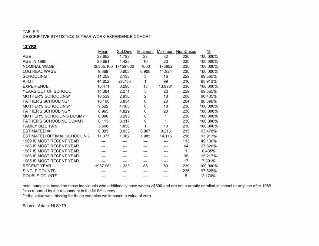
TABLE 5DESCRIPTIVE STATISTICS 13 YEAR WORK-EXPERIENCE COHORT

13 YRSMean Std.Dev. Minimum Maximum NumCases %

AGE 28.652 1.783 23 32 230 100.000%AGE IN 1980 20.691 1.425 16 23 230 100.000%NOMINAL WAGE 25355.100 17159.600 1000 173852 230 100.000%LOG REAL WAGE 9.869 0.603 6.908 11.924 230 100.000%SCHOOLING 11.258 2.138 3 16 229 99.565%AFQT 44.852 27.738 1 99 216 93.913%EXPERIENCE 13.471 0.296 13 13.9981 230 100.000%YEARS OUT OF SCHOOL 11.384 2.271 5 20 229 99.565%MOTHER'S SCHOOLING* 10.529 2.950 2 18 208 90.435%FATHER'S SCHOOLING* 10.108 3.834 0 20 204 88.696%MOTHER'S SCHOOLING** 9.522 4.183 0 18 230 100.000%FATHER'S SCHOOLING** 8.965 4.829 0 20 230 100.000%MOTHER'S SCHOOLING DUMMY 0.096 0.295 0 1 230 100.000%FATHER'S SCHOOLING DUMMY 0.113 0.317 0 1 230 100.000%FAMILY SIZE 1979 3.696 1.856 1 10 230 100.000%ESTIMATED r=I 0.095 0.033 0.007 0.216 215 93.478%ESTIMATED OPTIMAL SCHOOLING 11.377 1.362 7.985 14.116 216 93.913%1989 IS MOST RECENT YEAR --- --- --- --- 113 49.130%1988 IS MOST RECENT YEAR --- --- --- --- 64 27.826%1987 IS MOST RECENT YEAR --- --- --- --- 1 0.435%1986 IS MOST RECENT YEAR --- --- --- --- 35 15.217%1985 IS MOST RECENT YEAR --- --- --- --- 17 7.391%RECENT YEAR 1987.961 1.333 85 89 230 100.000%SINGLE COUNTS --- --- --- --- 225 97.826%DOUBLE COUNTS --- --- --- --- 5 2.174%

note: sample is based on those individuals who additionally have wages >$500 and are not currently enrolled in school or anytime after 1989*=as reported by the respondent in the NLSY survey**=if a value was missing for these variables we imposed a value of zero

Source of data: NLSY79

TABLE 6

MODEL/ESTIMATION STRAGEGY: UNRESTRICTED/OLS RESTRICTED/NLSURCOHORT: 13 YRS 13 YRS 13 YRS 13 YRS 13 YRS 13 YRS 13 YRS 13 YRS 13 YRS 13 YRS 13 YRSEQ: 14 15 17 19 19 22 22 15 17 19 22DEP. VARIAB.: ln(earnings) ln(earnings) estimated r estimated I estimated I years of school completed years of school completed ln(earnings) estimated r estimated I years of school completed

(1) (2) (3) (4) (5) (6) (7) (8) (9) (10) (11)CONSTANT 8.153 7.619 0.290 0.151 0.153 7.317 7.353 7.898 0.236 0.134 7.324

(45.311)** (14.426)** (2.965)** (14.764)** (4.023)** (13.449)** (2.406)** (35.786)** (6.049)** (8.086)** (14.652)**

SCHOOLING 0.153 0.290 -1.871E-02 --- --- --- --- 0.236 -1.395E-02 --- ---(9.722)** (2.965)** (-2.056)** (6.049)** (-2.927)**

AFQT*SCHOOLING --- 4.008E-04 --- --- --- --- --- 4.229E-04 --- --- ---(3.241)** (3.119)**

AFQT --- --- 4.008E-04 --- --- 3.089E-02 2.14E-02 --- 4.229E-04 --- 3.089E-02(3.241)** (6.738)** (2.659)** (3.119)** (6.004)**

SCHOOLING^2 --- -9.356E-03 --- --- --- --- --- -6.977E-03 --- --- ---(-2.056)** (-2.927)**

FATHER'S SCHOOLING --- --- --- -2.442E-03 -1.975E-03 0.106 0.115 --- --- -1.494E-03 0.107(-3.717)** (-2.064)** (2.862)** (1.455) (-1.995)* (2.840)**

MOTHER'S SCHOOLING --- --- --- -3.092E-03 -2.757E-03 0.147 0.159 --- --- -2.071E-03 0.148(-3.494)** (-1.919)* (3.088)** (1.580) (-2.161)** (3.882)**

FATHER'S SCHOOLING DUMMY --- --- --- -2.851E-02 -2.499E-02 1.335 1.385 --- --- -1.879E-02 1.347(-3.062)** (-1.856)* (2.659)** (1.496) (-2.010)** (2.904)**

MOTHER'S SCHOOLING DUMMY --- --- --- -1.089E-02 -9.796E-03 0.523 0.693 --- --- -7.354E-03 0.527(-.945) (-0.878) (.855) (0.772) (-.872) (.944)

FAMILY SIZE --- --- --- -3.895E-05 -5.542E-04 2.962E-02 9.533E-03 --- --- -3.897E-04 2.793E-02(-0.0354) (-0.0338) (0.495) (0.504) (-.481) (0.472)

R^2 0.294 0.299 --- 0.235 --- 0.446 --- 0.297 --- --- 0.446adj R^2 0.291 0.289 --- 0.216 0.281 0.430 --- --- --- --- ---resid. S.E. 0.507 0.477 --- 2.912E-02 2.506E-02 1.544 1.562 --- --- --- ---# observ. 229 215 215 215 215 215 215 215 215 215 215# of iterations --- --- --- --- --- --- --- 17 & 19 17 & 19 17 & 19 17 & 19Estimated at sample mean r=i --- --- 0.097 0.097 --- --- --- --- --- 0.095 ---Estimated at sample mean optimal years of schooling --- --- --- --- --- 11.377 11.377 --- --- --- 11.400

t-values are in parentheses** = significant at the 5% level for a 2 tailed t-test* = significant at the 10% level for a 2 tailed t-test

note:sample is based on those individuals who additionally have wages >$500 and are not currently enrolled in school or anytime after 1989(5)= derived form(7)=derived reduced form

Source of data: NLSY79

Technical Appendix

1. The interviewer established the respondent’s sex and race. An interviewer

only asked a respondent for his/her sex if it was not obvious by mere observation.

Furthermore, the “white” classification was established via the interviewer remarks.

The three choices available for race are white, black, and other. When the main data

files were merged with files from the work history supplements, it was done according

to the sex/race classifications as designated in the main files by the interviewer.

2. The family size is inclusive of the respondent and reflects his 1979 answers.

Ideally we would have liked to use the respondent’s family size when he was 14 years

old (this is how the Duncan Indices are established). However, due to the fact that

a large percentage of our respondents were between 18 and 22 years in the first year

of the survey, it is reasonable to expect that many of them lived on their own and

no longer took account of their family members when answering this question. We

tried to construct a better measure by using information on a respondent’s number

of siblings in 1979 and with whom he resided (i.e., parental units) when he was 14

years old. The data provided by the NLSY for the number of siblings seems pretty

unreasonable as it ranges from zero to 16. Most of the respondents report between

zero and five siblings, but there is a large number who report between six and eleven

siblings. Thus, when we calculate a respondent’s family size based on these measures

we get an average of 5.8 people, which is highly unlikely. We are left using the 1979

figures as reported by NLSY and concede that an average family size of 4.0 seems a

bit high as well.

3. There are several other IQ scores available, but the Otis-Lennon Mental Ability

Test was chosen because it had the most respondents.

4. The Knowledge of the World of Work (KWW) test was administered in 1979

and asks the respondents to pick which of three statements best describes a particular

42

job’s duties. An overall score is calculated by assigning a value of “1” to a correct

response and summing these for the nine questions.

5. The Department of Defense conducted the Armed Forces Qualifications Test

(AFQT) in 1980 to get a measure of trainability. The AFQT score is a composite

scored derived from select sections of the Armed Services Vocational Aptitude Battery

(ASVAB) test. The AFQT80 was calculated by summing the raw scores from the

arithmetic reasoning, word knowledge, paragraph comprehension, and one half the

numerical operations scores. The NLSY79 User’s Guide notes that the norms for the

AFQT are based on people who are at least 17 years old. Hence, those individuals

born in 1963 or 1964 were not used in this construction. They warn that while scores

have been constructed for these younger respondents, they have not been adjusted

to reflect their ages. But, the relative rankings of ability are maintained for all

respondents, regardless of their birth year.

6. The enrollment status as of May 1 for a given survey year was used because it

had the most observations available.

7. The NLSY79 reports these income variables for the past year. Hence, when

conducting the wage regressions for 1985 we use the total income from wages and

salary in the past year as reported in 1986.

8. The construction of the prior work experience inherently assumes that people’s

work experience in 1978 was similar to that measured in 1979.

9. There were two people in our sample who were 16 years old in 1979 and

reported 12 years of schooling completed. There were five others who were 17 years

old in 1979 and again reported having finished 12 years of school. All seven people

reported positive hours worked in 1979. Since our method of calculating prior work

experience would yield negative numbers for these individuals, we imposed a zero

value instead. This may underestimate these individuals prior work experience but

since this was so rare, we did not believe any serious bias would result.

43

10. For all the variables, except the hours worked, we left non-responses as missing

values. Observations with missing values were omitted from the analysis. However,

when considering the hours worked for a given year, we imputed a zero value for

anyone who did not respond to the question for whatever reason. The justification

for this is two-fold. First, we did not want a cumulative effect of missing observations.

So for example, if a respondent did not know how many hours he worked in 1980 but

did work 1,000 hours in 1981, we still wanted to consider him in our 1981 regressions.

Imposing a missing value for his 1980 hours worked would have eliminated him from

any future year analyses. Second, it seemed reasonable to assign a value of zero

rather than a missing value because the potential existed for the inapplicability of

this question for the respondent. This could be due to a person being unemployed

but actively searching for employment, entirely out of the labor force, in school, etc.

Thus any potential bias from this would be in the downward direction.

11. It was suggested that we randomly select samples of 157 observations from

each work-experience cohort and re-run (15) to get more comparable measures of

the “goodness of fit” criterion. Initially this sounded like a reasonable idea. Since

the 14-year work-experience cohort corresponded to the smallest sample size (i.e., 157

observations), we would just randomly resample from each of the previous cohorts and

see if the “overtaking” cohort did in fact change. However, upon greater reflection

we realized that the actual implementation of such an idea would involve an almost

prohibitively large number of regressions to run. Consider for example, how many

unique samples of 157 individuals would come from say the five-year work-experience

cohort of 1356 respondents! Moreover, it would be erroneous to use just one sample

of 157 respondents from each work-experience cohort to see if the “overtaking” cohort

changed based on the new selection criterion.

12. The occupational dummies used as instruments for AFQT include the follow-

ing: 1) professional, technical, and kindred workers; 2) managers and administrators,

44

except farm; 3) sales workers; 4) clerical and unskilled workers; 5) craftsmen and

kindred workers; 6) operatives, except transport; 7) transport equipment operatives;

8) laborers, except farm; 9) farmers and farm managers; 10) farm laborers and farm

foremen; 11) service workers, excluding private household; and 12) private household

workers.

45