a general high-order multi-domain hybrid dg/weno · pdf filehigh-order derivatives with the...
TRANSCRIPT

Journal of Computational Mathematics
Vol.34, No.1, 2016, 30–48.
http://www.global-sci.org/jcm
doi:10.4208/jcm.1510-m4512
A GENERAL HIGH-ORDER MULTI-DOMAIN HYBRIDDG/WENO-FD METHOD FOR HYPERBOLIC CONSERVATION
LAWS*
Jian Cheng, Kun Wang and Tiegang Liu
School of Mathematics and Systems Science, Beihang University, Beijing, China
Email: [email protected], [email protected], [email protected]
Abstract
In this paper, a general high-order multi-domain hybrid DG/WENO-FD method, which
couples a pth-order (p ≥ 3) DG method and a qth-order (q ≥ 3) WENO-FD scheme, is
developed. There are two possible coupling approaches at the domain interface, one is
non-conservative, the other is conservative. The non-conservative coupling approach can
preserve optimal order of accuracy and the local conservative error is proved to be upmost
third order. As for the conservative coupling approach, accuracy analysis shows the forced
conservation strategy at the coupling interface deteriorates the accuracy locally to first-
order accuracy at the ‘coupling cell’. A numerical experiments of numerical stability is
also presented for the non-conservative and conservative coupling approaches. Several
numerical results are presented to verify the theoretical analysis results and demonstrate
the performance of the hybrid DG/WENO-FD solver.
Mathematics subject classification: 65M60, 65M99, 35L65
Key words: Discontinuous Galerkin method, Weighted essentially nonoscillatory scheme,
Hybrid methods, high-order scheme.
1. Introduction
In recent years, high-order methods with low numerical diffusion and dispersion errors have
been extensively studied and widely used for resolving complex fluid structures and capturing
vortex evolution. Many kinds of high-order methods have been developed over the past two
decades, especially high-order finite difference (FD) type methods, such as weighted essentially
non-oscillatory (WENO) schemes [10, 11], high-order finite volume (FV) type methods [12, 29,
30] and discontinuous Galerkin (DG) type methods, which includes traditional Runge-Kutta
discontinuous Galerkin (RKDG) methods [1,2], spectral volume (SV) methods [19,20], spectral
difference (SD) method [14], correction procedure via reconstruction (CPR) schemes [13, 21]
and so on. FD type methods are generally considered as highly efficient and easily achieve
high-order accuracy on structured grids. FV type methods, compared to the FD type methods,
have flexibility in handling almost arbitrary grid with reasonable computational cost, however,
they usually are not compact when extends to high order accuracy. DG type methods can
treat complex geometries through a compact stencil as each cell only communicates with its
immediate face-neighbors through approximate Riemann solvers. However, they are generally
more time consuming than the FV type methods.
As all of those high-order methods mentioned above have their advantages and disadvan-
tages, several hybrid methods have been developed in order to locally take the advantages of
* Received April 18, 2014 / Revised version received June 22, 2015 / Accepted October 16, 2015 /
Published online January 18, 2016 /

A General High-Order Multi-Domain Hybrid DG/WENO-FD Method · · · 31
different types of methods above. There are mainly two kinds of hybrid approaches in literature,
one is based on local polynomial reconstruction, the other is based on computational domain
decomposition.
Based on local polynomial reconstruction, one of the most typical and successful imple-
mentation is WENO/Hermite WENO type limiter for DG methods [4–7]. The basic idea of
WENO/Hermite WENO limiter is to use the local polynomial reconstruction of WENO type to
replace the original reconstruction approach of DG methods for high-order degrees of freedom
at the ‘troubled cells’. Such hybrid approach preserves essentially non-oscillatory property for
those cells near the area of discontinuities. In fact, the strategy can be applied for all the
cells rather than only for those ‘troubled cells’. Luo et al. [3, 8, 9] adopted this strategy and
developed a kind of reconstructed DG methods (rDG) which reconstructs high-order degrees of
freedom using a least-squares technique in 2D and a hierarchial WENO reconstruction in 3D.
This hybrid approach combines the efficiency of reconstruction methods widely used in FV type
schemes and the accuracy and robustness of DG methods. Similarly, based on local polynomial
reconstruction, Dumbser et al. [15] presented a unified framework for constructing one step
finite volume and discontinuous Galerkin schemes on unstructured meshes, resulting in a class
of PnPm schemes. Zhang et al. [16–18] introduced a hybrid DG/FV method. In their hybrid
DG/FV method, a DG method based on Taylor basis functions was adopted to compute the
low-order degrees of freedom. A high order finite volume method is then used to reconstruct
high-order derivatives with the known low-order derivatives.
Based on computational domain decomposition, a multi-domain hybrid spectral-WENO
method was introduced by Costa et al. [22] for hyperbolic conservation laws. The hybrid
spectral-WENO method conjugates the non-oscillatory properties of high-order WENO schemes
and the high efficiency and accuracy of spectral methods in a multi-domain approach. Recently,
Shahbazi et al. [23] introduced a multi-domain Fourier-continuation/WENO hybrid solver for
conservation laws. In the area of CAA, Utzmann et al. [26,28] and Leger et al. [27] developed a
coupled DG/FD method for computational aeroacoustics. The coupled DG/FD solver approx-
imates the solution in the close neighborhood of complex obstacles with an unstructured grids
and computes the rest of the field on structured grids in order to alleviate computational cost.
In our previous work [31,32], we introduced a class of multi-domain hybrid DG and WENO-
FD method based on a third-order DG method and a fifth-order WENO-FD scheme for the
purpose of saving computational cost and treating complex geometry. We found that the con-
servative coupling approach deteriorates the accuracy seriously and only the non-conservative
coupling approach can preserve third-order accuracy. Thus, a special treatment was developed
in our previous work: the non-conservative coupling approach is employed when the solution is
smooth enough and it is replaced by the conservative coupling approach when there are possible
discontinuities passing through the interface.
In this paper, as a direct extension of our previous work, two main issues will be addressed:
one is whether the hybrid method can be extended to arbitrary high-order accuracy, the other is
whether the hybrid method can preserve numerical stability with different choices of numerical
fluxes at coupling interface. Firstly, we extend the previous third-order hybrid DG/WENO-FD
method to a more general situation which couples a pth-order (p ≥ 3) DG method with a qth-
order (q ≥ 3) WENO-FD scheme. We present a general analysis of accuracy and conservative
error for this general high-order hybrid DG/WENO-FD method. From the theoretical analysis,
as we will see later, the conservative coupling approach of a pth-order DG method and a qth-
order WENO-FD scheme is only of first-order accuracy locally at the ‘coupling cell’ and the

32 J. CHENG, K. WANG AND T.G. LIU
accuracy order is independent from the choices of numerical fluxes at the coupling interface. In
contrast, the non-conservative coupling approach can preserve optimal rth-order (r = min(p, q))
accuracy in the whole computational domain while at the same time the local conservative error
is proved to be upmost third order. Secondly, numerical analysis and comparison of stability for
the non-conservative and conservative coupling approaches is presented. Numerical experiments
demonstrate that the non-conservative coupling approach can preserve numerical stability. For
the conservative coupling approach, it can be seen that in some situation the conservative
coupling approach with WENO-FD flux employed at the coupling interface can lead to linear
instability. However, when the nonlinear factors are taken into consideration, both using DG
flux and using WENO-FD flux can preserve numerical stability.
The rest of this paper is arranged as follows. In Section 2, we give a detail description of the
general high-order hybrid DG/WENO-FD method. In Section 3, we present the general analysis
results of accuracy, stability and conservative error for the conservative and non-conservative
coupling approaches, respectively. In Section 4, numerical experiments of a hybrid 3rd-order
DG/5th-order WENO-FD method together with a hybrid 5th-order DG/5th-order WENO-FD
method are used to verify our theoretical results and demonstrate the performance of the high-
order hybrid solver. Finally, Section 5 contains concluding remarks.
2. A General High-order Hybrid DG/WENO-FD Method
In this section, we give a detail description of the high-order hybrid DG/WENO-FD method,
we will focus on the implementation for the scalar conservation law:
ut +d∑
i=1
(fi(u))xi = 0, (2.1)
where u = (u1, . . . , um)t, x = (x1, . . . , xd). For simplicity, we use the special case of (2.1) with
d = m = 1 as a model to illustrate the method. Assume that the computational domain
RKDG WENO-FD
coupling flux
a bJ + 1
2
... ...
- +
(a) Domain decomposition in one dimension.
RKDG WENO-FD
coupling flux
J + 1
2
ghost points
+-
(b) Ghost nodes for constructing the WENO-FD
flux of a 5th-WENO-FD scheme.
Fig. 2.1. Multi-domain hybrid methods for one dimensional problems.
a = x 12< x 3
2< · · · < xN+ 1
2= b,
as shown in Fig. 2.1(a), is divided into two subdomains with the multi-domain interface located
at x = xJ+1/2.
In the left subdomain (x1/2, xJ+1/2), a traditional high-order DG method is applied as
follows
du(l)j
dt+
1
wl
[△−
(vjl (xj+ 1
2)f
(rkdg)
j+ 12
)]− 1
wl
∫Ij
f(uh(x, t))d
dxvjl (x)dx = 0, l = 0, 1, 2, · · · , k,
(2.2)
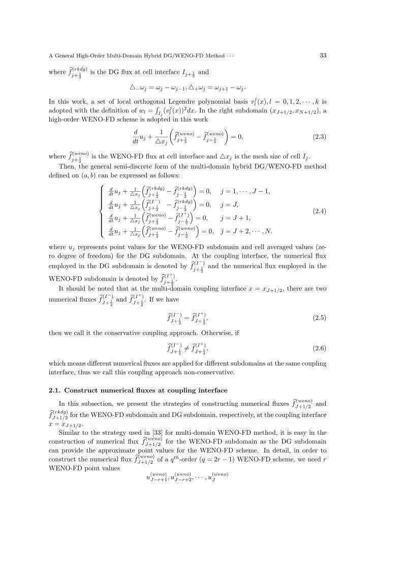
A General High-Order Multi-Domain Hybrid DG/WENO-FD Method · · · 33
where f(rkdg)
j+ 12
is the DG flux at cell interface Ij+ 12and
△−ωj = ωj − ωj−1,△+ωj = ωj+1 − ωj .
In this work, a set of local orthogonal Legendre polynomial basis vjl (x), l = 0, 1, 2, · · · , k is
adopted with the definition of wl =∫Ij(vjl (x))
2dx. In the right subdomain (xJ+1/2, xN+1/2), a
high-order WENO-FD scheme is adopted in this work
d
dtuj +
1
△xj
(f(weno)
j+ 12
− f(weno)
j− 12
)= 0, (2.3)
where f(weno)
j+ 12
is the WENO-FD flux at cell interface and △xj is the mesh size of cell Ij .
Then, the general semi-discrete form of the multi-domain hybrid DG/WENO-FD method
defined on (a, b) can be expressed as follows:
ddtuj +
1△xj
(f(rkdg)
j+ 12
− f(rkdg)
j− 12
)= 0, j = 1, · · · , J − 1,
ddtuj +
1△xj
(f(I−)
j+ 12
− f(rkdg)
j− 12
)= 0, j = J,
ddtuj +
1△xj
(f(weno)
j+ 12
− f(I+)
j− 12
)= 0, j = J + 1,
ddtuj +
1△xj
(f(weno)
j+ 12
− f(weno)
j− 12
)= 0, j = J + 2, · · · , N.
(2.4)
where uj represents point values for the WENO-FD subdomain and cell averaged values (ze-
ro degree of freedom) for the DG subdomain. At the coupling interface, the numerical flux
employed in the DG subdomain is denoted by f(I−)
j+ 12
and the numerical flux employed in the
WENO-FD subdomain is denoted by f(I+)
j+ 12
.
It should be noted that at the multi-domain coupling interface x = xJ+1/2, there are two
numerical fluxes f(I−)
J+ 12
and f(I+)
J+ 12
. If we have
f(I−)
J+ 12
= f(I+)
J+ 12
, (2.5)
then we call it the conservative coupling approach. Otherwise, if
f(I−)
J+ 12
= f(I+)
J+ 12
, (2.6)
which means different numerical fluxes are applied for different subdomains at the same coupling
interface, thus we call this coupling approach non-conservative.
2.1. Construct numerical fluxes at coupling interface
In this subsection, we present the strategies of constructing numerical fluxes f(weno)J+1/2 and
f(rkdg)J+1/2 for the WENO-FD subdomain and DG subdomain, respectively, at the coupling interface
x = xJ+1/2.
Similar to the strategy used in [33] for multi-domain WENO-FD method, it is easy in the
construction of numerical flux f(weno)J+1/2 for the WENO-FD subdomain as the DG subdomain
can provide the approximate point values for the WENO-FD scheme. In detail, in order to
construct the numerical flux f(weno)J+1/2 of a qth-order (q = 2r − 1) WENO-FD scheme, we need r
WENO-FD point values
u(weno)J−r+1, u
(weno)J−r+2, · · · , u
(weno)J
34 J. CHENG, K. WANG AND T.G. LIU
at xJ−r+1, xJ−r+2, · · · , xJ , which are located in the DG subdomain and called ghost points.
For example, we show these ghost points used for constructing the numerical flux for a 5th-
order WENO-FD scheme in Fig. 2.1(b). These point values are simply calculated from the
approximate solution polynomial of a pth-order DG method:
uh(x, t) =
p−1∑l=0
u(l)j (t)φ
(j)l (x), x ∈ Ij , (2.7)
where u(l)j (t) are degrees of freedom in the cell Ij and φ
(j)l (x), l = 0, 1, · · · p− 1 are a set of local
orthogonal basis over Ij .
As for the constructing of the numerical flux f(rkdg)J+1/2 for the DG subdomain, we need get
u+J+1/2 and u−
J+1/2 at the coupling interface xJ+1/2 to form the numerical flux. It is obvious
that u−J+1/2 at the right boundary of the cell IJ can be obtained by expression (2.7), whereas,
u+J+1/2 needs to be reconstructed through the point values from the WENO-FD subdomain.
In order to preserve high order accuracy and prevent possible numerical oscillation, a WENO
type interpolation is applied to the construction of u+J+1/2. In this procedure, we need a stencil
of 2p − 1 points to obtain the Gauss quadrature point values and reconstruct the degrees of
freedom for a pth-order DG method in the target cell IJ+1. To do so, the following steps are
used:
Step 1: Choose 2p − 1 points interpolation stencil S = {IJ−p+2, · · · , IJ+p−1, IJ+p} and
divide stencil S into p small stencils denoted by
Si = {IJ−p+2+i, · · · , IJ+i, IJ+1+i}, i = 0, 1, · · · , p− 1;
Step 2: Construct an interpolation polynomial pi(x) associated with each of the stencils
Si, i = 0, 1, · · · , p− 1 which satisfied pi(xk) = u(xk), k ∈ Si and get these approximate point
values at each Gauss quadrature point xG in the cell IJ+1 of each pi(x), i = 0, 1, · · · , p− 1;
Step 3: Obtain the linear weights λi, smoothness indicators βi and calculate the nonlin-
ear weights ωi of each small stencil Si, i = 0, 1, · · · , p − 1 following WENO reconstruction
procedures, the final approximate for each Gauss quadrature point xG is then given by
u(xG) ≈p−1∑i=0
ωipi(xG), xG ∈ IJ+1; (2.8)
Step 4: Reconstruct the degrees of freedom for the DG method in the cell IJ+1 through a
numerical integration
u(l)J+1 =
1
al
∑G
wGu(xG)φ(J+1)l (xG), l = 0, 1, · · · , p− 1, (2.9)
where al =∑
G wG(φ(J+1)l (xG))
2. Then, get the u+J+1/2 through the expression (2.7).
Since we have reconstructed the u+J+1/2 at the right side of the coupling interface x = xJ+1/2,
we can form the DG numerical flux f(rkdg)J+1/2 for the DG subdomain. The advantages of using
WENO interpolation in constructing DG flux is that WENO interpolation can provide u+J+1/2
with the property of essentially non-oscillation. It should be noted that this is crucial in
preserving the numerical stability when the DG flux is employed at the coupling interface. Al-
ternatively, we can get u+J+1/2 directly through a WENO interpolation at the coupling interface

A General High-Order Multi-Domain Hybrid DG/WENO-FD Method · · · 35
x = xJ+1/2 instead of reconstruction the approximated solution polynomial in the cell IJ+1.
Numerical experiments demonstrate that actually there is not much difference in obtaining
u+J+1/2 directly from this WENO interpolation, thus we also use this simple strategy in some
of our numerical experiments.
2.2. Non-conservative and conservative coupling
As the numerical fluxes at the coupling interface are not unique, we have two kinds of
coupling approaches at the coupling interface, one is non-conservative, the other is conservative.
For the non-conservative approach, we use different numerical fluxes for different subdomains
at the same coupling interface x = xJ+1/2. More specifically, we use
f(I−)
J+ 12
= f(rkdg)
J+ 12
, f(I+)
J+ 12
= f(weno)
J+ 12
, (2.10)
for the non-conservative coupling approach and the semi-discrete form Eq. (2.4) becomesddtuj +
1△xj
(f(rkdg)
j+ 12
− f(rkdg)
j− 12
)= 0, j = 1, · · · , J,
ddtuj +
1△xj
(f(weno)
j+ 12
− f(weno)
j− 12
)= 0, j = J + 1, · · · , N.
(2.11)
Non-conservative coupling approach demonstrates good performance when the solution is
smooth nearby the coupling interface, however, if there is a discontinuity, such as a shock wave,
like most of the other non-conservative methods, this coupling approach might suffer from a
severe problem in capturing discontinuities correctly. At this moment, conservative coupling
approach must be employed at the coupling interface. For this conservative coupling, we can
use either the WENO-FD flux or the DG flux as the unique flux at the coupling interface and
the semi-discrete form Eq. (2.4) of the conservative coupling approach now becomes
ddtuj +
1△xj
(f(rkdg)
j+ 12
− f(rkdg)
j− 12
)= 0, j = 1, · · · , J − 1,
ddtuj +
1△xj
(f(I)
j+ 12
− f(rkdg)
j− 12
)= 0, j = J,
ddtuj +
1△xj
(f(weno)
j+ 12
− f(I)
j− 12
)= 0, j = J + 1,
ddtuj +
1△xj
(f(weno)
j+ 12
− f(weno)
j− 12
)= 0, j = J + 2, · · · , N.
(2.12)
where f(I)
J+ 12
= f(rkdg)
J+ 12
or f(I)
J+ 12
= f(weno)
j+ 12
.
2.3. Hybrid DG/WENO-FD method
The theoretical analysis in the next section will show that there are both advantages and
disadvantages for non-conservative and conservative approaches. In practical application, we
firstly detect possible discontinuities near the coupling interface, then choose the appropriate
coupling approach in the hybrid DG/WENO-FD method.
In order to detect those possible discontinuities near the coupling interface x = xJ+1/2, a
feasible way is to use the so-called ‘troubled cell’ indicator [4,5]. We call a cell ‘troubled cell’ if
the cell is indicated to possibly include a discontinuity. Thus, if either of the neighbor cells near
the coupling interface is identified as a ‘troubled cell’, it is wise to use the conservative coupling
approach rather than the non-conservative one. That means the hybrid method comes back to
be conservative when a discontinuity is passing through the coupling interface. In practice, we

36 J. CHENG, K. WANG AND T.G. LIU
follow our previous work [31, 32] and use a TVD(TVB) minmod function as the ‘troubled cell’
indicator as follow
u(mod)k = m(uk,△+uk,△−uk), ˜u(mod)
k = m(˜uk,△+uk,△−uk), k = J, J + 1 (2.13)
where uk = u−k+ 1
2
−uk, ˜uk = uk−u+k− 1
2
, △+uk = uk+1−uk, △−uk = uk−uk−1 and m(a1, a2, a3)
is the TVD (TVB) minmod function. It should be noted that for the RKDG subdomain, the
zero degree of freedom u(0)k is used as the cell average uk and for the WENO-FD subdomain, the
cell average uk is provided by the high order integration polynomial p(x) described in Section
2.1.
Finally, we summary the procedure of the multi-domain hybrid DG/WENO-FD method in
following steps:
Step 1: Initialize degrees of freedom for the DG subdomain and point values for the WENO-
FD subdomain;
Step 2: Construct numerical fluxes f(weno)J+1/2 and f
(rkdg)J+1/2 at the coupling interface, respectively;
Step 3: Detect the possible discontinuities in the neighbor cells IJ and IJ+1 of the cou-
pling interface: If neither of these two neighbor cells is identified as a ‘troubled cell’, the
non-conservative coupling approach is adopted; Otherwise, the conservative coupling approach
is applied with an unique numerical flux f(weno)I+1/2,J or f
(rkdg)I+1/2,J used at the coupling interface;
Step 4: Complete the space discretization for the DG subdomain and the WENO-FD sub-
domain.
As for the time discretization, an explicit third-order TVD Runge-Kutta method is used
with a CFL number equal to the minimum of the CFL numbers of all the subdomains. It
should be noticed that the strategy of choosing CFL is straight forward, however, may be not
optimal, as for real application, a local time stepping procedure should be more appropriate.
Finally, the third-order TVD Runge-Kutta method is given as follows
u(1) = un +∆tL(un), (2.14a)
u(2) =3
4un +
1
4u(1) +
1
4∆tL(u(1)), (2.14b)
un+1 =1
3un +
2
3u(2) +
2
3∆tL(u(2)). (2.14c)
3. Accuracy, Stability and Conservative Error
In this section, we will present some theoretical analysis about the multi-domain hybrid
DG and WENO-FD method described in Section 2. For the conservative coupling approach,
analysis of accuracy and stability will be presented in Subsection 3.1. We also give a comparison
between the two different choices, using the DG flux or using the WENO-FD flux, as the unique
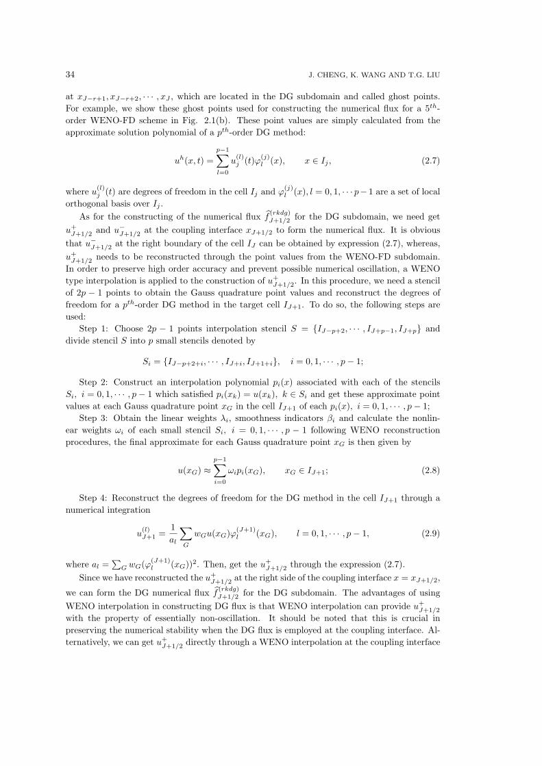
numerical flux at the coupling interface as shown in Fig. 3.1(a) and Fig. 3.1(b). For the non-
conservative coupling approach, analysis of accuracy and conservative error will be presented
in Subsection 3.2.
3.1. Conservative coupling approach
In the conservative coupling approach, an unique flux needs to be defined at the coupling
interface. This can easily be done by simply choosing the numerical flux of either the DG
method or the WENO-FD scheme provided at the interface. Another simple way is to use an

A General High-Order Multi-Domain Hybrid DG/WENO-FD Method · · · 37
RKDG WENO-FD
DG flux
J
WENO type coupling cell
J + 1
- + + +- -
(a) Use DG flux as interface flux.
RKDG WENO-FD
WENO flux
J
DG type coupling cell
J + 1
- + + +- -
(b) Use WENO-FD flux as interface flux.
Fig. 3.1. Different choices of numerical flux at the coupling interface for conservative coupling.
exact or approximate Riemann problem solution to define a unique numerical flux since the
left and right flow states at the coupling interface are readily provided by the DG and WENO
methods. In this work, we simply take either the DG flux or the WENO-FD flux as the unique
flux at coupling interface. If we apply the DG flux at the coupling interface x = xJ+1/2 as shown
in Fig. 3.1(a), a so-called WENO type ‘coupling cell’ will be generated in the cell IJ+1 which
means the space discretization in the cell IJ+1 is employed by WENO-FD schemes, however,
the numerical flux of left boundary of this cell comes from DG method. In a similar way, if a
WENO-FD flux is chosen as the unique flux at x = xJ+1/2, the ‘coupling cell’ will be located in
the cell IJ with a DG discretization actually applied in it, we denote it as a DG type ‘coupling
cell’ as shown in Fig. 3.1(b).
3.1.1. Accuracy analysis
We note that the space discretization in the coupling cell with these two different choices of
numerical fluxes shown in Fig. 3.1(a) and Fig. 3.1(b), however, leads to a similar form. In
specific, if the DG flux is employed at the coupling interface, the semi-discrete scheme for the
WENO-FD point value uJ+1 in the cell IJ+1 follows
d
dtuJ+1 +
1
△xJ+1(f
(weno)
J+ 32
− f(rkdg)
J+ 12
) = 0. (3.1)
Conversely, if the WENO-FD flux is used, the semi-discrete scheme for the DG cell average
value uJ in the cell IJ has the form
d
dtuJ +
1
△xJ(f
(weno)
J+ 12
− f(rkdg)
J− 12
) = 0. (3.2)
Eq. (3.1) and Eq. (3.2) indicate that the accuracy of conservative hybrid DG/WENO-FD
method in the coupling cell is independent from the choices of different numerical fluxes at the
coupling interface. For the accuracy analysis, we have the following theorem.
Theorem 3.1. The semi-discrete scheme of the conservative coupling of a pth-order (p ≥ 3)
DG method and a qth-order (q ≥ 3) WENO-FD scheme is of first order accuracy locally in the
coupling cell in the norm L∞.
Proof. To evaluate the numerical flux of a qth-order WENO-FD scheme, we assign λk is
the linear weight and pk is the reconstructed polynomials of the candidate stencil Sk (k =
0, 1, · · · , r − 1, q = 2r − 1).

38 J. CHENG, K. WANG AND T.G. LIU
Then we have
f(weno)
J+ 32
= hJ+ 32+O(∆xq), (3.3)
where the definition of h(x) is according to Shu and Osher [24,25]:
f(x) =1
∆x
∫ x+∆x/2
x−∆x/2
h(ξ)dξ. (3.4)
For the pth-order DG method, using Taylor series expansion at the center of the cell IJreveals the following formula at the coupling interface
f(rkdg)
J+ 12
= fJ+ 12+O(∆xp). (3.5)
From Eq. (3.3) and Eq. (3.5), the space discretization in the cell IJ+1 can be rewritten as
f(weno)
J+ 32
− f(rkdg)
J+ 12
= hJ+ 32− fJ+ 1
2+O(∆xmin(p,q)). (3.6)
From Shu and Osher [24,25], we know that the relationship between hJ+ 32and fJ+ 3
2is
hJ+ 32= fJ+ 3
2− 1
24
d2f
dx2
∣∣∣∣x=x
J+32
∆x2 +O(∆x4). (3.7)
Eq. (3.7) indicates that
f(weno)
J+ 32
− f(rkdg)
J+ 12
= fJ+ 32− fJ+ 1
2+O(∆x2). (3.8)
Thus, the semi-discrete scheme of the conservative hybrid approach in the coupling cell is of
first order accuracy and the accuracy is independent from the choices of numerical fluxes used
at the interface. �
Remark 3.1. Although, the conservative semi-discrete scheme in the coupling cell is of first-
order accuracy, an O(∆x2) solution error is routinely observed for the whole computation
domain in numerical experiments after applying time discretization.
3.1.2. Stability
In this subsection, we present analysis of stability for the conservative coupling approach
through numerical tests. The two different choices of numerical fluxes at the coupling in-
terface do not exert much influence on the accuracy. Nevertheless, numerical experiments show
that the stability of the conservative coupling approach in some degree depends on the choices
of numerical fluxes.
In our numerical experiments, the linear scalar hyperbolic conservation law is used as ex-
amples and the computational domain is directly divided into two subdomains. We test both
linear and nonlinear situation for the conservative coupling approach. Linear conservative cou-
pling approach means that the nonlinear limiter of the DG method and nonlinear weights of the
WENO-FD scheme are not taken into consideration. In contrast, the nonlinear conservative
coupling approach indicates that the nonlinear factors may exert their influence in solving a
linear conservation law.
From our numerical results, it has been found that the using of DG flux at the coupling
interface for conservative coupling approach can preserve numerical stability well for both linear

A General High-Order Multi-Domain Hybrid DG/WENO-FD Method · · · 39
and nonlinear situation. However, the choice of using WENO-FD flux at the coupling interface
may lead to linear instability in some situation. In order to preserve numerical stability for
this case, nonlinear factors in the DG method and the WENO-FD scheme must be taken into
consideration. The details of the numerical results are shown in Table 3.1.
Table 3.1: Stability of conservative coupling approach.
Left subdomain: DG Right subdomain: WENO-FD
Use DG flux at coupling interface Use WENO-FD flux at coupling interface
f ′(u) > 0 f ′(u) < 0 f ′(u) > 0 f ′(u) < 0
linear√ √
×√
nonlinear√ √ √ √
Left subdomain: WENO-FD Right subdomain: DG
Use DG flux at coupling interface Use WENO-FD flux at coupling interface
f ′(u) > 0 f ′(u) < 0 f ′(u) > 0 f ′(u) < 0
linear√ √ √
×nonlinear
√ √ √ √
3.2. Non-conservative coupling approach
For the non-conservative coupling approach, we give theoretical results of accuracy and local
conservative error. The conclusion of accuracy analysis is directly given by the theorem ?? as
the reconstruction steps are applied at the coupling interface, the fact that the non-conservative
coupling approach can preserve high order accuracy for smooth solutions becomes obvious.
3.2.1. Accuracy analysis
The semi-discrete scheme of the non-conservative coupling of a pth-order (p ≥ 3) DG method
and a qth-order (q ≥ 3) WENO-FD scheme can preserve optimal rth-order(r = min{p, q})accuracy in the region of smooth solutions.
3.2.2. Conservative error
A significant concern of a non-conservative method is the conservative error (CE). Here, we use
following formula to evaluate the local conservative error:
CE =
∣∣∣∣∑j
△xjun+1j −
∑j
△xjunj
∣∣∣∣, (3.9)
where unj is the numerical solution of time Tn. If a one dimensional scheme is truly conservative
with periodic boundary conditions or limj→±∞ u0j = 0 is imposed, then the conservative error
is equal to zero. For the non-conservative multi-domain hybrid DG/WENO-FD method, we
give an analysis based on the definition above.
Theorem 3.2. The local conservative error for the non-conservative coupling of a pth-order
(p ≥ 3) DG method and a qth-order (q ≥ 3) WENO-FD scheme is of third order accuracy.
Proof. From Eq. (2.11), we haveun+1j = un
j − ∆t∆x (f
n(rkdg)
j+ 12
− fn(rkdg)
j− 12
), j = 1, · · · , J,
un+1j = un
j − ∆t∆x (f
n(weno)
j+ 12
− fn(weno)
j− 12
), j = J + 1, · · · , N.(3.10)
40 J. CHENG, K. WANG AND T.G. LIU
Multiply (3.10) by ∆x and sum over all cells with the assumption that j → 1 and j → N ,
u0j → 0, we obtain ∑
j
∆xun+1j −
∑j
∆xunj = −∆t
(fn(rkdg)
J+ 12
− fn(weno)
J+ 12
). (3.11)
As we known from theorem 3.1,∣∣∣fk(rkdg)
J+ 12
− fk(weno)
J+ 12
∣∣∣ = O(∆x2). (3.12)
Thus, the conservative error of the non-conservative hybrid method is of third-order accuracy. �
3.2.3. Stability
The strict theoretical analysis of stability for the non-conservative coupling approach may be
complex and tedious. However, we can look at this problem from another point. As the DG
method and WENO-FD scheme are both numerical stable, if we can preserve the property of
essentially non-oscillatory in the reconstruction of numerical fluxes at the coupling interface,
then the non-conservative coupling approach should preserve numerical stability. From the
procedures of reconstructing numerical fluxes presented in Section 2.1, it should be noted that
the WENO type reconstruction is applied to preserve the property of essentially non-oscillatory.
Numerical experiments also demonstrate the non-conservative coupling approach is stable.
4. Numerical Results
In this section, we will present several numerical results of our high-order multi-domain hy-
brid DG/WENO-FD method. Two hybrid DG/WENO-FD methods are provided in Subsection
4.1 to verify the theoretical results for the conservative and non-conservative hybrid approach-
es, one is a hybrid 3rd-order DG/5th-order WENO-FD method, the other is a hybrid 5th-order
DG/5th-order WENO-FD method. Then, typical cases of two dimensional scalar conservation
law and Euler equations are presented to demonstrate the performance of our high-order hybrid
solvers in Subsection 4.2 and 4.3.
4.1. One dimensional conservation law
4.1.1. Accuracy test
Example 4.1. We solve the linear advection equation with the following initial and exact
boundary conditions: {ut − ux = 0,
u(x, 0) = sin(π(x+ 0.25)).x ∈ (0.0, 2.0), (4.1)
In this test case, we display the accuracy results of the semi-discrete scheme for conservative
coupling approach. In specific, a linear conservative coupling of third-order DG and fifth-
order WENO-FD, together with a linear conservative coupling of fifth-order DG and fifth-order
WENO-FD are demonstrated as examples. It should be noted that here compared to nonlinear
coupling, linear coupling means the nonlinear factors, such as limiters in the DG subdomain and
the nonlinear weights in the WENO-FD subdomain are not taken into account. The subdomain

A General High-Order Multi-Domain Hybrid DG/WENO-FD Method · · · 41
Table 4.1: Accuracy test of the conservative coupling approach locally at the ‘coupling cell’ (Example
4.1).
Use DG flux at coupling interface Use WENO-FD flux at coupling interface
3rd-DG/5th-WENO-FD5th-DG/5th-WENO-FD3rd-DG/5th-WENO-FD5th-DG/5th-WENO-FD
N L∞ error L∞ order L∞ error L∞ order L∞ error L∞ order L∞ error L∞ order
40 1.45E-2 1.45E-2 1.62E-2 1.66E-2
80 7.27E-3 1.00 7.27E-3 1.00 7.71E-3 1.07 7.82E-3 1.09
160 3.63E-3 1.00 3.63E-3 1.00 3.75E-5 1.04 3.77e-3 1.05
320 1.82E-3 1.00 1.82E-3 1.00 1.85E-5 1.02 1.85e-3 1.03
interface is set at x = 1.0, where the DG method is applied in (0.0, 1.0) and the WENO-FD
scheme is applied in (1.0, 2.0). At the coupling interface, we test both using the DG flux and
using the WENO-FD flux as the unique flux for this conservative coupling approach. The results
are shown in Table 4.1. Through the numerical results, we can see that the conservative semi-
discrete coupling is locally first-order accuracy at the coupling cell and the order is independent
from the choices of numerical fluxes at the coupling interface.
Example 4.2. We solve the linear advection equation with the following initial and exact
boundary conditions: {ut − ux = 0,
u(x, 0) = sin(π(x+ 0.25)).x ∈ (0.0, 2.0), (4.2)
In this test case, we display the results of a linear conservative coupling of third-order DG and
the fifth-order WENO-FD, together with a linear conservative coupling of fifth-order DG and
fifth-order WENO-FD. All the set are the same as Example 4.1. The computing time is till
1.0. At the coupling interface, we test both using the DG flux and using the WENO-FD flux
as the unique flux for this conservative coupling approach. The results are shown in Table 4.2.
Through the numerical results, we can see that the conservative coupling approach is numerical
stable and shows upmost second-order accuracy in the whole computation domain and the order
of accuracy is independent from the choices of numerical fluxes at the coupling interface.
Table 4.2: Accuracy test of linear conservative coupling approach (Example 4.2).
Use DG flux at coupling interface
3rd-DG/5th-WENO-FD 5th-DG/5th-WENO-FD
N L∞ error L∞ order L1 error L1 order L∞ error L∞ order L1 error L1 order
40 1.02E-3 6.43E-4 1.03E-3 6.51E-4
80 2.56E-4 1.99 1.62E-4 1.99 2.57E-4 2.00 1.63E-4 2.00
160 6.42E-5 2.00 4.07E-5 1.99 6.42E-5 2.00 4.09e-5 1.99
320 1.61E-5 2.00 1.02E-5 2.00 1.61E-5 2.00 1.02e-5 2.00
Use WENO-FD flux at coupling interface
3rd-DG/5th-WENO-FD 5th-DG/5th-WENO-FD
N L∞ error L∞ order L1 error L1 order L∞ error L∞ order L1 error L1 order
40 1.05E-3 6.58E-4 1.06E-3 6.67E-4
80 2.58E-4 2.02 1.64E-4 2.00 2.58E-4 2.04 1.65E-4 2.02
160 6.42E-5 2.01 4.10E-5 2.00 6.43E-5 2.00 4.11e-5 2.01
320 1.61E-5 2.00 1.02E-5 2.01 1.61E-5 2.00 1.02e-5 2.01

42 J. CHENG, K. WANG AND T.G. LIU
Example 4.3. We solve the linear advection equation with the following initial and exact
boundary conditions: {ut + ux = 0,
u(x, 0) = sin(π(x+ 0.25)).x ∈ (0.0, 2.0), (4.3)
In this test case, the characteristics propagate in an opposite direction compared to Example
4.1. We also display the results of a linear conservative coupling of third-order DG and fifth-
order WENO-FD, together with a linear conservative coupling of fifth-order DG and fifth-order
WENO-FD. All the other settings are the same as Example 4.1. The results are shown in Table
4.3. In this case, numerical results show that the linear conservative coupling approach which
uses the DG flux at the coupling interface is stable and exhibit a second-order convergence.
However, the conservative coupling approach which adopts the WENO-FD flux suffers numerical
instability during the numerical experiment. In order to preserve the stability, nonlinear factors
must be considered as shown in Subsection 4.1.3.
Table 4.3: Accuracy test of linear conservative coupling approach (Example 4.3).
Use DG flux at the coupling interface
3rd-DG/5th-WENO-FD 5th-DG/5th-WENO-FD
N L∞ error L∞ order L1 error L1 order L∞ error L∞ order L1 error L1 order
40 1.03E-3 6.44E-4 1.03E-3 6.42E-4
80 2.57E-4 2.00 1.62E-4 1.99 2.57E-4 2.00 1.62E-4 1.99
160 6.43E-5 2.00 4.07E-5 1.99 6.42E-5 2.00 4.07E-5 1.99
320 1.61E-5 2.00 1.02E-5 2.00 1.61E-5 2.00 1.02E-5 2.00
Example 4.4. We solve the same linear advection equation using non-conservative coupling
approach with the following initial and exact boundary conditions:{ut ± ux = 0,
u(x, 0) = sin(π(x+ 0.25)).x ∈ (0.0, 2.0), (4.4)
In this example, we test the accuracy of the non-conservative coupling approach. All the
other settings are same as Example 4.1. The results are shown in Table 4.4. As we seen
Table 4.4: Accuracy test of linear non-conservative coupling approach (Example 4.4).
3rd-DG/5th-WENO-FD
ut + ux = 0 ut − ux = 0
N L∞ error L∞ order L1 error L1 order L∞ error L∞ order L1 error L1 order
40 1.91E-5 1.40E-5 2.01E-5 1.39E-5
80 2.06E-5 3.21 1.80E-6 2.96 2.08E-6 3.27 1.76E-6 2.98
160 2.57E-5 3.00 2.27E-7 2.99 2.57E-7 3.02 2.24E-7 2.97
320 3.21E-5 3.00 2.83E-8 3.00 3.21E-8 3.00 2.82E-8 2.99
5th-DG/5th-WENO-FD
ut + ux = 0 ut − ux = 0
N L∞ error L∞ order L1 error L1 order L∞ error L∞ order L1 error L1 order
40 4.67E-6 1.40E-6 3.56E-6 1.33E-6
80 1.53E-7 4.93 4.15E-8 5.08 1.29E-7 4.79 6.11E-8 4.44
160 4.92E-9 4.96 1.27E-9 5.03 4.01E-9 5.01 1.89E-9 5.01
320 1.58E-10 4.96 4.00E-11 4.95 1.25E-10 5.00 5.97E-11 4.98

A General High-Order Multi-Domain Hybrid DG/WENO-FD Method · · · 43
from the numerical results, the non-conservative coupling approach are numerical stable and
can preserve optimal order of accuracy. More specifically, a third-order convergence and a fifth-
order convergence are exhibited by a non-conservative coupling of a third-order DG method with
a fifth-order WENO-FD scheme and a non-conservative coupling of a fifth-order DG method
with a fifth-order WENO-FD scheme, respectively.
Example 4.5. We solve the Burgers’ equation with the following initial and periodic boundary
conditions: {ut + (u
2
2 )x = 0,
u(x, 0) = 0.5 + sin(πx).x ∈ (0.0, 2.0), (4.5)
In this test case, we display the accuracy tests for both the conservative coupling approach and
non-conservative coupling approach. The computational domain has been divided into three
subdomains where the DG method is in (0.5, 1.5) and the WENO-FD scheme is applied in
(0.0, 0.5) and (1.5, 2.0). Periodic boundary is imposed and the computing time is till T = 0.5/π
when the solution is still smooth. The results are shown in Table 4.5 and 4.6. Similarly, we ob-
serve that conservative coupling approach shows only second-order of accuracy and the accuracy
is independent from the choices of numerical fluxes at the coupling interfaces. In contrast, the
non-conservative coupling approach demonstrates a good performance in preserving high-order
accuracy.
Table 4.5: Accuracy test of conservative coupling approach (Example 4.5).
Use DG flux at the coupling interface
3rd-DG/5th-WENO-FD 5th-DG/5th-WENO-FD
N L∞ error L∞ order L∞ error L∞ order L∞ error L∞ order L∞ error L∞ order
40 1.04E-3 2.79E-4 9.95E-4 1.13E-4
80 2.79E-4 1.90 3.08E-5 2.13 2.86E-4 1.80 2.79E-5 2.02
160 6.99E-5 2.00 7.31E-6 2.07 7.50E-5 1.93 6.96E-6 2.01
320 1.78E-5 1.96 1.79E-6 2.03 1.81E-5 2.05 1.73E-5 2.01
Use WENO-FD flux at the coupling interface
3rd-DG/5th-WENO-FD 5th-DG/5th-WENO-FD
N L∞ error L∞ order L1 error L1 order L∞ error L∞ order L1 error L1 order
40 1.19E-3 1.72E-4 1.15E-3 1.58E-4
80 3.34E-4 1.83 3.58E-5 2.27 3.32E-4 1.79 3.26E-4 2.27
160 8.48E-5 1.98 7.89E-6 2.18 8.61E-5 1.95 7.41E-5 2.14
320 2.10E-5 2.01 1.85E-6 2.01 1.81E-5 2.25 1.73E-5 2.10
Table 4.6: Accuracy test of non-conservative coupling approach (Example 4.5).
3rd-DG/5th-WENO-FD 5th-DG/5th-WENO-FD
N L∞ error L∞ order L1 error L1 order L∞ error L∞ order L1 error L1 order
40 1.47E-4 1.73E-5 2.29E-6 3.15E-7
80 2.56E-5 2.53 2.53E-6 2.77 7.66E-8 4.90 5.85E-9 5.75
160 3.61E-6 2.83 3.51E-7 2.85 8.45E-10 6.50 1.42E-10 5.36
320 4.80E-7 2.91 4.61E-8 2.93 2.55E-11 5.05 4.32E-12 5.05

44 J. CHENG, K. WANG AND T.G. LIU
4.1.2. Conservative error
Example 4.6. We solve the linear advection equation with the following initial and periodic
boundary conditions: {ut ± ux = 0,
u(x, 0) = sin(π(x+ 0.25)).x ∈ (0.0, 2.0), (4.6)
In this test case, we display the local conservative error of a non-conservative coupling of
third-order DG and fifth-order WENO-FD, together with a non-conservative coupling of fifth-
order DG and fifth-order WENO-FD. In order to impose periodic boundary conditions, the
computational domain has been divided into three subdomains as Example 4.5. The results
are shown in Table 4.7. From the numerical results, we can find out that the local conservative
error is third-order which verifies our theoretical analysis.
Table 4.7: Local conservative error test of non-conservative coupling approach (Example 4.6).
3rd-DG/5th-WENO-FD 5th-DG/5th-WENO-FD
ut + ux = 0 ut − ux = 0 ut + ux = 0 ut − ux = 0
N L∞ error L∞ order L∞ error L∞ order L∞ error L∞ order L∞ error L∞ order
40 8.40E-6 8.40E-6 2.31E-6 2.31E-6
80 1.04E-6 3.01 1.03E-6 3.02 2.89E-7 3.00 2.89E-7 3.00
160 1.30E-7 3.00 1.30E-7 3.00 3.61E-8 3.00 3.61E-8 3.00
320 1.63E-8 3.00 1.63E-8 3.00 4.52E-9 3.00 4.52E-9 3.00
4.1.3. Stability
Example 4.7. We solve the linear advection equation with the following initial and exact
boundary conditions: {ut + ux = 0,
u(x, 0) = sin(π(x+ 0.25)).x ∈ (0, 2), (4.7)
This test case is the same as Example 4.3 in which the numerical results show that it is lin-
ear unstable if WENO-FD flux is employed as the unique flux for the conservative coupling
approach. In order to preserve numerical stability, the conservative coupling approach has to
be nonlinear even for solving linear conservation law. When the nonlinear factors are taken
into consideration, the conservative coupling using WENO-FD flux at coupling interface can
preserve numerical stability and the numerical results are shown in Table 4.8.
Table 4.8: Stability test of conservative coupling approach (Example 4.7).
Use WENO-FD flux at the coupling interface
3rd-DG/5th-WENO-FD 5th-DG/5th-WENO-FD
N L∞ error L∞ order L1 error L1 order L∞ error L∞ order L1 error L1 order
40 3.46e-3 8.27e-4 4.72e-3 2.47e-3
80 1.31e-3 1.40 1.97e-4 2.06 1.20e-3 1.98 6.21e-4 1.99
160 4.07e-4 1.69 4.61e-5 2.09 3.05e-4 1.98 1.56e-5 1.99
320 8.22e-5 2.30 1.07e-5 2.11 7.69e-5 1.99 3.90e-6 2.00

A General High-Order Multi-Domain Hybrid DG/WENO-FD Method · · · 45
4.2. Two dimensional conservation law
Example 4.8. We further test the performance of the multi-domain hybrid DG/WENO-FD
method for solving two dimensional inviscid Burgers’ equation with the following initial and
periodic boundary conditions. The subdomain interfaces occur at x = 0.5, 0.0 < y < 2.0 and
x = 1.5, 0.0 < y < 2.0. The computing time is till 0.5/π and 1.5/π. At T = 0.5/π, the
solution is still smooth. We display the L∞ and L1 errors of a hybrid method of third-order
DG coupling fifth-order WENO-FD together with a hybrid method of fifth-order DG coupling
fifth-order WENO-FD, respectively. Numerical results show the hybrid methods can preserve
high-order accuracy in Table 4.9. At T = 1.5/π, the numerical results illustrate that shock
waves can correctly pass through the coupling interface as shown in Fig. 4.1.{ut + (u
2
2 )x + (u2
2 )y = 0,
u(x, 0) = 0.5 sin(π(x+ y)) + 0.25.(x, y) ∈ (0.0, 2.0)× (0.0, 2.0), (4.8)
Table 4.9: Accuracy test of hybrid DG/WENO-FD methods (Example 4.8).
3rd-DG/5th-WENO-FD 5th-DG/5th-WENO-FD
N×N L∞ error L∞ order L1 error L1 order L∞ error L∞ order L1 error L1 order
40×40 4.54e-4 2.96e-5 1.52e-4 2.95e-6
80×80 5.10e-5 3.15 2.99e-6 3.31 9.60e-6 3.98 5.29e-8 5.80
160×160 3.44e-6 3.89 3.64e-7 3.11 3.93e-7 4.61 9.74e-10 5.76
320×320 4.90e-7 2.81 4.88e-8 2.90 1.03e-8 5.25 2.24e-11 5.44
X
Y
0 0.5 1 1.5 20
0.5
1
1.5
2
(a) Hybrid 3rd-DG/5th-WENO-FD method, mesh
size h = 1/160.
X
Y
0 0.5 1 1.5 20
0.5
1
1.5
2
(b) Hybrid 5th-DG/5th-WENO-FDmethod, mesh
size h = 1/160.
Fig. 4.1. Two dimensional Burgers’ equation at time T = 1.5/π.
4.3. Two dimensional Euler equations
We consider the two dimensional Euler equations
Ut + F (U)x +G(U)y = 0, (4.9)where
U = (ρ, ρu, ρv, E)T , F (U) = (ρu, ρu2 + P, ρuv, u(E + P ))T ,
G(U) = (ρv, ρuv, ρv2 + P, u(E + P ))T .

46 J. CHENG, K. WANG AND T.G. LIU
(a) 3rd-DG method, 30 density contours from 1.731 to 20.92, mesh
size h = 1/120, CPU time: 17059.6s
(b) Hybrid 3rd-DG/5th-WENO-FD method, 30 density contours
from 1.731 to 20.92, mesh size h = 1/120, CPU time: 10238.7s
(c) 5th-DG method, 30 density contours from 1.731 to 20.92, mesh
size h = 1/120, CPU time: 75534.6s
(d) Hybrid 5th-DG/5th-WENO-FD method, 30 density contours
from 1.731 to 20.92, mesh size h = 1/120, CPU time: 39921.2s
Fig. 4.2. Double mach reflection problem.
The total energy E is expressed as
E =P
γ − 1+
1
2ρ(u2 + v2), (4.10)
with γ = 1.4 for air.
Example 4.9. This is a standard test case for high resolution schemes. The computational
domain is chosen to be (0.0, 4.0)×(0.0, 1.0). Initially a right-moving Mach 10 shock is positioned
at x = 1/6, y = 0.0 and makes a 60o angle with the x-axis. The coupling interface is located
at y = 0.25, 0.0 < x < 4.0 with DG method computing 25% regions of total domain near
A General High-Order Multi-Domain Hybrid DG/WENO-FD Method · · · 47
the bottom. A comparison of the hybrid 3rd-order DG/5th-order WENO-FD method and the
hybrid 5th-order DG/5th-order WENO-FD method is presented in Fig. 4.2. From the numerical
results, we can see that both the third-order and the fifth-order hybrid DG/WENO-FD method
give good performances in handling the coupling interface in this test case. From the CPU time
comparison, it can be seen clearly that the hybrid method is much more efficient than traditional
pure DG method.
5. Conclusions
In this paper, a general high-order multi-domain hybrid DG/WENO-FD method which
couples a pth-order (p ≥ 3) DG method and a qth-order (q ≥ 3) WENO-FD scheme has been
developed. The conservative and non-conservative coupling approaches were described in detail.
We concluded that the conservative coupling approach is only of first-order accuracy locally at
the ‘coupling cell’. In contrast, the non-conservative coupling approach can preserve the optimal
order in the whole computation domain while the local conservative error is upmost third order.
As for the stability analysis, numerical experiments showed nonlinear factors must be taken into
consideration in order to maintain the stability for the conservative coupling approach when the
WENO-FD flux is employed at the coupling interface. Further research focusing on extension
the hybrid solver to diffusion equations is ongoing.
Acknowledgments. This work is supported by the Innovation Foundation of BUAA for PhD
Graduates, the National Natural Science Foundation of China (Nos. 91130019 and 10931004),
the International Cooperation Project (No. 2010DFR00700), the State Key Laboratory of
Software Development Environment (No. SKLSDE-2011ZX-14) and the National 973 Project
(No. 2012CB720205).
References
[1] B. Cockburn, Discontinuous Galerkin methods for convection-dominated problems, High-order
methods for computational physics, Springer Berlin Heidelberg, Springer, 1999.
[2] B. Cockburn, C.-W. Shu, The Runge-Kutta local projection discontinuous Galerkin finite element
method for scalar conservation laws V: Multidimensional systems, J. Comput. Phys., 141(1998),
199-224.
[3] H. Luo, Y.D. Xia, S. Spiegel, R. Nourgaliev, Z. L. Jiang, A reconstructed discontinuous Galerkin
method based on a Hierarchical WENO reconstruction for compressible flows on tetrahedral grids,
J. Comput. Phys., 236(2013), 477-492.
[4] J.X. Qiu, C.-W. Shu, Runge-Kutta discontinuous Galerkin method using WENO limiters, SIAM
J. Sci. Comput., 26(2005), 907-929.
[5] J.X. Qiu, C.-W. Shu, Hermite WENO schemes and their application as limiter for Runge-Kutta
discontinuous Galerkin method: One dimensional case, J. Comput. Phys., 193(2004), 115-135.
[6] J. Zhu, J.X. Qiu, Hermite WENO schemes and their application as limiter for Runge-Kutta
discontinuous Galerkin method III: Unstructured meshes, J. Sci. Comput., 39(2009), 293-321.
[7] H. Luo, J.D. Baum, R. Lohner, A Hermite WENO-based limiter for discontinuous Galerkin method
on unstructed grids, AIAA-2007-0510.
[8] H. Luo, Y. Xia, R. Nourgaliev, C. Cai, A Class of reconstructed discontinuous galerkin methods
for the compressible flows on arbitrary grids, AIAA-2011-0199.
[9] H. Luo, H. Xiao, R. Nourgaliev, C. Cai, A comparative study of different reconstruction schemes
for reconstructed discontinuous Galerkin methods for the compressible flows on arbitrary grids,
AIAA-2011-3839.
[10] G.S. Jiang, C.-W. Shu, Efficient implementation of weighted ENO schemes, J. Comput. Phys.,
126(1996), 202-228.

48 J. CHENG, K. WANG AND T.G. LIU
[11] D. Balsara, C.-W. Shu, Monotonicity preserving weighted essentially non-oscillatory schemes with
increasingly high order of accuracy, J. Comput. Phys., 160(2000), 405C452.
[12] O. Friedrich, Weighted essentially non-oscillatory schemes for the interpolation of mean values on
unstructured grids, J. Comput. Phys., 144(1998), 194-212.
[13] Z.J. Wang, H.Y. Gao, A unifying lifting collocation penalty formulation including the discon-
tinuous Galerkin, spectral volume/difference methods for conservation laws on mixed grids, J.
Comput. Phys., 228(2009), 8161-8186.
[14] Y. Liu, M. Vinokur, Z.J. Wang, Discontinuous spectral difference method for conservation laws
on unstructured grids, J. Compout. Phys., 216(2006), 780-801.
[15] M. Dumbser, D.S. Balsara, E.F. Toro, A unified framework for the construction of one step finite
volume and discontinuous Galerkin schemes on unstructed meshes, J. Comput. Phys., 227(2008),
8209-8253.
[16] L.P. Zhang, W. Liu, L.X. He, X.G. Deng, H.X. Zhang, A new class of DG/FV hybrid methods for
conservation laws I: Basic formulation and one-dimensional systems, J. Comput. Phys., 231(2012),
1081-1103.
[17] L.P. Zhang, W. Liu, L.X. He, X.G. Deng, H.X. Zhang, A class of hybrid DG/FV methods for
conservation laws II: Two dimensional cases, J. Comput. Phys., 231(2012), 1104-1120.
[18] L.P. Zhang, W. Liu, L.X. He, X.G. Deng, A class of hybrid DG/FV methods for conservation laws
III: Two dimensional Euler Equations, Commun. Comput. Phys., 12(2012), 284-314.
[19] Z.J. Wang, Spectral (Finite) volume method for conservation laws on unstructured grids: basic
formulation, J. Comput. Phys., 178(2002), 210-251.
[20] Z.J. Wang, Y. Liu, Spectral (Finite) volume method for conservation laws on unstructured grids
IV: extension to two-dimensional systems, J. Comput. Phys., 194(2004), 716-741.
[21] H.T. Huynh, A flux reconstruction approach to high-order schemes including discontinuous
Galerkin methods, AIAA-2007-4079.
[22] B. Costa, W.S. Don, Multi-domain hybrid spectral-WENO methods for hyperbolic conservation
laws, J. Comput. Phys., 224(2007), 970-991.
[23] K. Shahbazi, N. Albin, O.P. Bruno, J.S. Hesthaven, Multi-domain Fourier-continuation/WENO
hybrid solver for conservation laws, J. Comput. Phys., 230(2011), 8779-8796.
[24] C.-W. Shu, S. Osher, Efficient implementation of essentially non-oscillatory shock capturing
schemes I, J. Comput. Phys., 77(1987), 439-471.
[25] C.-W. Shu, S. Osher, Efficient implementation of essentially non-oscillatory shock capturing
schemes II, J. Comput. Phys., 83(1989), 32-78.
[26] J. Utzmann, F. Lorcher, M. Dumbser, C.-D. Munz, Aeroacoutic simulations for complex geome-
tries based on hybrid meshes, AIAA-2006-2418.
[27] R. Leger, C. Peyret, Coupled discontinuous Galerkin/Finite Difference solver on hybrid meshes
for computational aeroacoutics, AIAA JOURNAL 50(2012), 338-349.
[28] J. Utzmann, T. Schwartzkopff, M. Dumbser, C.-D. Munz, Heterogeneous domain decomposition
for CAA, AIAA-2005-2989.
[29] P. Tsoutsanis, V.A. Titarev, D. Drikakis, WENO schemes on arbitrary mixed-element unstruc-
tured meshes in three space dimensions, J. Comput. Phys., 230(2011), 1585-1601.
[30] M. Dumbser, M. Kaser, Arbitrary high order non-oscillatory finite volume schemes on unstructured
meshes for linear hyperbolic systems, J. Comput. Phys., 221(2007), 693-723.
[31] J. Cheng, Y.W. Lu, T.G. Liu, Multi-domain hybrid RKDG and WENO methods for hyperbolic
conservation laws, SIAM J. Sci. Comput., 35(2013), A1049-A1072.
[32] J. Cheng, T.G. Liu, A multi-domain hybrid DG and WENO method for hyperbolic conservation
laws on hybrid mesh, Commun. Comput. Phys., 16(2014), 1116-1134.
[33] K. Sebastian and C.-W. Shu, Multidomain WENO finite difference method with interpolation at
subdomain interfaces, J. Sci. Comput., 19(2003), 405-438.