a galerkin boundary element method for …sms03snc/convpoly_final_revised.pdf · a galerkin...
TRANSCRIPT

A GALERKIN BOUNDARY ELEMENT METHOD FOR HIGH
FREQUENCY SCATTERING BY CONVEX POLYGONS
S N CHANDLER-WILDE∗† AND S LANGDON∗‡
Abstract. In this paper we consider the problem of time-harmonic acoustic scattering in twodimensions by convex polygons. Standard boundary or finite element methods for acoustic scatteringproblems have a computational cost that grows at least linearly as a function of the frequency ofthe incident wave. Here we present a novel Galerkin boundary element method, which uses anapproximation space consisting of the products of plane waves with piecewise polynomials supportedon a graded mesh, with smaller elements closer to the corners of the polygon. We prove thatthe best approximation from the approximation space requires a number of degrees of freedom toachieve a prescribed level of accuracy that grows only logarithmically as a function of the frequency.Numerical results demonstrate the same logarithmic dependence on the frequency for the Galerkinmethod solution. Our boundary element method is a discretisation of a well-known second kindcombined-layer-potential integral equation. We provide a proof that this equation and its adjointare well-posed and equivalent to the boundary value problem in a Sobolev space setting for generalLipschitz domains.
Key words. Galerkin boundary element method, high frequency scattering, convex polygons,Helmholtz equation, large wave number, Lipschitz domains
AMS subject classifications. 35J05, 65R20
1. Introduction. The scattering of time-harmonic acoustic waves by boundedobstacles is a classical problem that has received much attention in the literatureover the years. Much effort has been put into the development of efficient numericalschemes, but an outstanding question yet to be fully resolved is how to achieve anaccurate approximation to the scattered wave with a reasonable computational costin the case that the scattering obstacle is large compared to the wavelength of theincident field.
The standard boundary or finite element method approach is to seek an approxi-mation to the scattered field from a space of piecewise polynomial functions. However,due to the oscillatory nature of the solution, such an approach suffers from the limita-tion that a fixed number of degrees of freedom K are required per wavelength in orderto achieve a good level of accuracy, with the accepted guideline in the engineering lit-erature being to take K = 10 (see for example [53] and the references therein). Afurther difficulty, at least for the finite element method, is the presence of “pollutionerrors”, phase errors in wave propagation across the domain, which can lead to evenmore severe restrictions on the value of K when the wavelength is short [9, 39].
Let L be a linear dimension of the scattering obstacle, and set k = 2π/λ, whereλ is the wavelength of the incident wave, so that k is the wave number, proportionalto the frequency of the incident wave. Then a consequence of fixing K is that thenumber of degrees of freedom will be proportional to (kL)d, where d = N in thecase of the finite element method (FEM), d = N − 1 in the case of the boundaryelement method (BEM), and N = 2 or 3 is the number of space dimensions of theproblem. Thus, as either the frequency of the incident wave or the size of the obstaclegrows, so does the number of degrees of freedom, and hence the computational cost of
∗Department of Mathematics, University of Reading, Whiteknights, PO Box 220, Berkshire RG66AX, UK
†Email: [email protected]‡Supported by a Leverhulme Trust Early Career Fellowship. Email: [email protected]
1

2 S. N. CHANDLER-WILDE AND S. LANGDON
the numerical scheme. As a result, the numerical solution of many realistic physicalproblems is intractable using current technologies. In fact, for some of the mostpowerful recent algorithms for three-dimensional scattering problems (e.g. [13, 21]),the largest obstacles for which numerical results have been reported have diameternot more than a few hundred times the wavelength.
For boundary element methods, the cost of setting up and solving the large lin-ear systems which arise can be reduced substantially through a combination of pre-conditioned iterative methods [4, 22, 36] combined with fast matrix-vector multiplymethods based on the fast multipole method [5, 26, 21] or the FFT [13]. However,this does nothing to reduce the growth in the number of degrees of freedom as kL in-creases (linear with respect to kL in 2D, quadratic in 3D). Thus computations becomeinfeasible as kL→ ∞.
1.1. Reducing the number of degrees of freedom for kL large. To achievea dependence of the number of degrees of freedom on kL which is lower than (kL)d, itseems essential to use an approximation space better able to replicate the behaviourof the scattered field at high frequencies than piecewise polynomials. To that end,much attention in the recent literature has focused on enriching the approximationspace with oscillatory functions, specifically plane waves or Bessel functions.
A common approach (see e.g. [8, 16, 27, 37, 53]) is to form an approximationspace consisting of standard finite element basis functions multiplied by plane wavestravelling in a large number of directions, approximately uniformly distributed on theunit circle (in 2D) or sphere (in 3D). Theoretical analysis (e.g. [8]) and computationalresults (e.g. [53]) suggest that these methods converge rapidly as the number of planewave directions increases, with a significant reduction in the number of degrees offreedom required per wavelength, compared to standard finite and boundary elementmethods. But the number of degrees of freedom is still proportional to (kL)d, andserious conditioning problems occur when the number of plane wave directions is large.
A related idea is to attempt to identify the important wave propagation directionsat high frequencies, and to incorporate the oscillatory part of this high frequencyasymptotic behaviour into the approximation space. This is the idea behind the finiteelement method of [34] and the boundary element methods of [25, 19, 12, 33, 45]. Thisidea has been investigated most thoroughly in the case that the scattering obstacleis smooth and strictly convex. In this case the leading order oscillatory behaviour isparticularly simple on the boundary of the scattering obstacle, so that this approach isperhaps particularly well-adapted for boundary element methods. If a direct integralequation formulation is used, in which the solution to be determined is the trace ofthe total field or its normal derivative on the boundary, the most important wavedirection to include is that of the incident wave (see for example [1, 25, 12, 28]). Thisapproach is equivalent, in the case of a sound hard scatterer, to approximating theratio of the total field to the incident field, with physical optics predicting that thisratio is approximately constant on the illuminated side and approximately zero onthe shadow side of the obstacle at high frequencies.
In [1], Abboud et. al. consider the two dimensional problem of scattering by asmooth, strictly convex obstacle. They suggest that the ratio of the scattered fieldto the incident field can be approximated with error of order N−ν + ((kL)1/3/N)ν+1
using a uniform mesh of piecewise polynomials of degree ν, so that the total numberof degrees of freedom N only needs to be proportional to (kL)1/3 in order to maintaina fixed level of accuracy. In fact this paper appears to be the first in which the depen-dence of the error estimates on the wave number k is indicated, and the requirement

HIGH FREQUENCY SCATTERING BY CONVEX POLYGONS 3
that the number of degrees of freedom is proportional to (kL)1/3 is a big improvementover the usual requirement for proportionality to kL. This approach is coupled witha fast multipole method in [25], where impressive numerical results are reported forlarge scale 3D problems.
The same approach is combined with a mesh refinement concentrating degrees offreedom near the shadow boundary in [12]. The numerical results in [12] for scatteringby a circle suggest that, with this mesh refinement, both the number of degreesof freedom and the total computational cost required to maintain a fixed level ofaccuracy remain constant as kL→ ∞. The method of [12] has recently been appliedto deal with each of the multiple scatters which occur when a wave is incident ontwo, separated, smooth convex 2D obstacles [33]. Numerical experiments have alsorecently been presented in [29] where the convergence of this iterative approach tothe multiple scattering problem is analysed.
In [28] a numerical method in the spirit of [12] is proposed, namely a p-versionboundary element method with a k-dependent mesh refinement in a transition regionaround the shadow boundary. A rigorous error analysis, which combines estimatesusing high frequency asymptotics of derivatives of the solution on the surface withcareful numerical analysis, demonstrates that the approximation space is able to rep-resent the oscillatory solution to any desired accuracy provided the number of degreesof freedom increases approximately in proportion to (kL)1/9 as kL increases. And infact numerical experiments in [28], using this approximation space as the basis of aGalerkin method, suggest that a prescribed accuracy can be achieved by keeping thenumber of degrees of freedom fixed as the wave number increases.
The boundary element method and its analysis that we will present in this paperfor the problem of scattering by a convex polygon are most closely related to our ownrecent work [19, 45] on the specific problem of 2D acoustic scattering by an inhomo-geneous, piecewise constant impedance plane. In [19, 45] a Galerkin boundary ele-ment method for this problem is proposed, in which the leading order high frequencybehaviour as k → ∞, consisting of the incident and reflected ray contributions, isfirst subtracted off. The remaining scattered wave, consisting of rays diffracted bydiscontinuities in impedance, is expressed as a sum of products of oscillatory andnon-oscillatory functions, with the non-oscillatory functions being approximated bypiecewise polynomials supported on a graded mesh, with larger elements away fromdiscontinuities in impedance. For the method in [19] it was shown in that paper thatthe number of degrees of freedom needed to maintain accuracy as k → ∞ grows onlylogarithmically with k. This result was improved in [45] where it was shown, viasharper regularity results and a modified mesh, that for a fixed number of degrees offreedom the error is bounded independently of k.
1.2. The oscillatory integral problem. In the above paragraphs we havereviewed methods for reducing the dependence on k of the number of degrees offreedom necessary to achieve a required accuracy. Indeed some of the methods we havedescribed above [12, 45, 33, 28] appear, in numerical experiments, to require only anumber of degrees of freedomM = O(1) as k → ∞. Further, for one specific scatteringproblem [45] this has been shown by a rigorous numerical analysis. However, it shouldbe emphasised strongly that this is not the end of the story; M = O(1) as k → ∞does not imply a computational cost which is O(1) as k → ∞. The reason is that,while M fixed implies a fixed size of the approximating linear system, the matrixentries become increasingly difficult to evaluate, at least by conventional quadraturemethods, as k → ∞. This observation is perhaps particularly true for boundary

4 S. N. CHANDLER-WILDE AND S. LANGDON
integral equation based methods where the difficulty arises from the high frequencybehaviour of both the oscillatory basis functions (necessary to keepM fixed as k → ∞)and the oscillatory kernels of the integral operators. As a consequence, each matrixentry is a highly oscillatory integral when k is large. We discuss only briefly in thispaper the effective evaluation of the matrix entries in the Galerkin method we willpropose, referring the reader to [44] for most of the details. And the methods wedescribe in [44] are O(1) in computational cost as k → ∞ for many but not all of thematrix entries, so that further work is required to make the algorithm we will proposefully effective at high frequency. But we note that, of the papers cited above, onlythe methods of Bruno et al. [12, 33] and Langdon and Chandler-Wilde [45] appear toachieve an O(1) computational cost as k → ∞.
The issue in evaluating the matrix entries is one of numerical evaluation of oscil-latory integrals. In Bruno et al. this is achieved by a ‘localized integration’ strategydescribed in [12]. This strategy might be termed a ‘numerical method of station-ary phase’, in which the integrals are approximated by localised integrals over small,wave-number-dependent neighbourhoods of the stationary points of the oscillatoryintegrand. A similar strategy for integrals of the same type arising in high fre-quency boundary integral methods for 3D problems is developed in [32]. Promis-ing alternative approaches are two older methods for oscillatory integrals due toFilon [31] (recently re-analysed by Iserles [40, 41] and see [6] for discussion of itsapplication to the matrix entries in a high-frequency collocation boundary elementmethod) and Levin [47], and methods based on deformation of paths of integrationinto the complex plane to steepest descent paths [38]. We note that, in contrast to[12, 33, 6], where Nystrom/collocation methods are used and the oscillatory integralsare one-dimensional, the matrix entries in our Galerkin methods are, of course, two-dimensional oscillatory integrals, so that development of a robust method for theirevaluation is a harder problem.
1.3. The main results of the paper. In this paper, we consider specificallythe problem of scattering by convex polygons. This is, in at least one respect, a morechallenging problem than the smooth convex obstacle since the corners of the polygongive rise to strong diffracted rays which illuminate the shadow side of the obstaclemuch more strongly than the rays that creep into the shadow zone of a smooth convexobstacle. These creeping rays decay exponentially, so that it is enough to remove theoscillation of the incident field to obtain a sufficiently simple field to approximate bypiecewise polynomials, though a wave number dependent, carefully graded mesh (cf.[12, 28]) must be used to resolve the transition zone between illuminated and shadowregions.
This approach, of removing the oscillation of the incident field and then approx-imating by a piecewise polynomial, does not suffice for a scatterer with corners. Inbrief, our algorithm for the convex polygon is as follows, inspired by our previouslydeveloped algorithm for scattering by a piecewise-constant impedance plane [19], dis-cussed in the last paragraph of §1.1. From the geometrical theory of diffraction, oneexpects, on the sides of the polygon, incident, reflected and diffracted ray contribu-tions. On each illuminated side, the leading order behaviour as k → ∞ consists ofthe incident wave and a known reflected wave. The first stage in our algorithm is toseparate this part of the solution explicitly. (On sides in shadow this step is omitted.)The remaining field on the boundary consists of waves which have been diffracted atthe corners and which travel along the polygon sides. We approximate this remainingfield by taking linear combinations of products of piecewise polynomials with plane

HIGH FREQUENCY SCATTERING BY CONVEX POLYGONS 5
waves, the plane waves travelling parallel to the polygon sides. A key ingredient inour algorithm is to design a graded mesh to go on each side of the polygon for thepiecewise polynomial approximation. This mesh has larger elements away from thecorners and a mesh grading near the corners depending on the internal angles, in sucha way as to equidistribute the approximation error over the subintervals of the mesh,based on a careful study of the oscillatory behaviour of the solution.
The major results of the paper are as follows. We begin in §2 by introducingthe exterior Dirichlet scattering problem that we will solve numerically via a sec-ond kind boundary integral equation formulation. Our boundary integral equation iswell known (e.g. [23]), obtained from Green’s representation theorem. The boundaryintegral operator is a linear combination of a single-layer potential and its normalderivative, so that the integral equation is precisely the adjoint of the equation pro-posed independently for the exterior Dirichlet problem by Brakhage and Werner [11],Leis [46], and Panic [52]. However, it seems (see e.g. the introduction to [14]) notto be widely appreciated that these formulations are well-posed for Lipschitz as wellas smooth domains in a range of boundary Sobolev spaces; indeed there exists onlya brief and partial account of these standard formulations for the Lipschitz domaincase in the literature [50] (the treatment in [23] is for domains of class C2). Weremedy this gap in the literature in §2, showing that our operator is a bijection onthe boundary Sobolev space Hs−1/2(Γ) and the adjoint operator of [11] a bijection onHs+1/2(Γ), both for |s| ≤ 1/2. Our starting points are known results on the (Laplace)double-layer potential operator on Lipschitz domains [57, 30] coupled with mappingproperties of the single-layer potential operator [49]. (We note that this obvious ap-proach of deducing results for the Helmholtz equation as a perturbation from theLaplace case has previously been employed for second kind boundary integral equa-tions in Lipschitz domains in [56, 50, 48].) Of course the results we obtain apply inparticular to a polygonal domain in 2D.
The design of our numerical algorithm depends on a careful analysis of the oscilla-tory behaviour of the solution of the integral equation (which is the normal derivativeof the total field on the boundary Γ). This is the content of §3 of the paper. Incontrast e.g. to [28], where this information is obtained by difficult high frequencyasymptotics, we adapt a technique from [19, 45], where explicit representations of thesolution in a half-plane are obtained from Green’s representation theorem. In theestimates we obtain of high order derivatives, we take care to obtain as precise infor-mation as possible, with a view to the future design of alternative numerical schemes,perhaps based on a p- or hp-boundary element method.
Section 4 of the paper contains, arguably, the most significant theoretical andpractical results. In this section we design an approximation space for the normalderivative of the total field on Γ. As outlined above, on each side we approximatethis unknown as the sum of the leading order asymptotics (known explicitly, and zeroon a side in shadow) plus an expression of the form exp(iks)V+(s) + exp(−iks)V−(s),where s is arc-length distance along the side and V±(s) are piecewise polynomials.We show, as a main result of the paper, that the approximation space based on thisrepresentation has the property that the error in best approximation of the normalderivative of the total field is bounded by Cν(n[1 + log(kL)])ν+3/2M−ν−1
N , where MN
is the total number of degrees of freedom, L is the length of the perimeter, n thenumber of sides of the polygon, ν is the polynomial degree, and the constant Cν
depends only on ν and the corner angles of the polygon. This is a strong result,showing that the number of degrees of freedom need only increase like log3/2(kL) as

6 S. N. CHANDLER-WILDE AND S. LANGDON
kL→ ∞ to maintain accuracy.
In §5 we analyse a Galerkin method, based on the approximation space of §4.We show that the same bound holds for our Galerkin method approximation to thesolution of the integral equation, except that an additional stability constant is intro-duced. We do not attempt the (difficult) task of ascertaining the dependence of thisstability constant on k. In §6 we present some numerical results which fully supportour theoretical estimates, and we discuss, briefly, some numerical implementation is-sues, including conditioning and evaluation of the integrals that arise. We finish thepaper with some concluding remarks and open problems.
We note that the Galerkin method is, of course, not the only way to select anumerical solution from a given approximation space. In [6] we present some results fora collocation method, based on the approximation space results in §4. The attractionof the Galerkin method we present in §5 is that we are able to establish stability, atleast in the asymptotic limit of sufficient mesh refinement, which we do not know howto do for the collocation method.
2. The boundary value problem and integral equation formulation.
Consider scattering of a time-harmonic acoustic plane wave ui by a sound-soft convexpolygon Υ, with boundary Γ :=
⋃nj=1 Γj , where Γj , j = 1, . . . , n are the n sides of
the polygon with j increasing anticlockwise, as shown in figure 2.1. We denote by
Υ
ui
P1 n1
Γ1
Ω1
P2
n2Γ2
Ω2
P3
n3Γ3 Ω3
P4
n4
Γ4
Ω4P5
n5
Γ5
Ω5
P6
n6
Γ6
Ω6
θ
Fig. 2.1. Our notation for the polygon.
Pj := (pj , qj), j = 1, . . . , n, the vertices of the polygon, and we set Pn+1 = P1, sothat, for j = 1, . . . , n, Γj is the line joining Pj with Pj+1. We denote the length ofΓj by Lj := |Pj+1 − Pj |, the external angle at each vertex Pj by Ωj ∈ (π, 2π), theunit normal perpendicular to Γj and pointing out of Υ by nj := (nj1, nj2), and theangle of incidence of the plane wave, as measured anticlockwise from the downwardvertical, by θ ∈ [0, 2π). Writing x = (x1, x2) and d := (sin θ,− cos θ), we then have
ui(x) = eik(x1 sin θ−x2 cos θ) = eikx·d.
We will say that Γj is in shadow if nj · d ≥ 0 and is illuminated if nj · d < 0. If ns isthe number of sides in shadow, it is convenient to choose the numbering so that sides1, . . . , ns are in shadow, sides ns + 1, . . . , n are illuminated.

HIGH FREQUENCY SCATTERING BY CONVEX POLYGONS 7
We will formulate the boundary value problem we wish to solve for the totalacoustic field u in a standard Sobolev space setting. For an open set G ⊂ RN ,let H1(G) := v ∈ L2(G) : ∇v ∈ L2(G) (∇v denoting here the weak gradientof v). We recall [49] that, if G is a Lipschitz domain then there is a well-definedtrace operator, the unique bounded linear operator γ : H1(G) → H1/2(∂G) whichsatisfies γv = v|∂G in the case when v ∈ C∞(G) := w|G : w ∈ C∞(RN ). LetH1(G; ∆) := v ∈ H1(G) : ∆v ∈ L2(G) (∆ the Laplacian in a weak sense), a Hilbertspace with the norm ‖v‖H1(G;∆) :=
∫
G[|v|2 + |∇v|2 + |∆v|2]dx1/2. If G is Lipschitz,
then [49] there is also a well-defined normal derivative operator, the unique boundedlinear operator ∂n : H1(G; ∆) → H−1/2(∂G) which satisfies
∂nv =∂v
∂n:= n · ∇v,
almost everywhere on Γ, when v ∈ C∞(G). H1loc(G) denotes the set of measurable
v : G→ C for which χv ∈ H1(G) for every compactly supported χ ∈ C∞(G).The polygonal domain Υ is Lipschitz as is its exterior D := R2 \ Υ. Let γ+ :
H1(D) → H1/2(Γ) and γ− : H1(Υ) → H1/2(Γ) denote the exterior and interior traceoperators, respectively, and let ∂+
n : H1(D; ∆) → H−1/2(Γ) and ∂−n : H1(Υ; ∆) →H−1/2(Γ) denote the exterior and interior normal derivative operators, respectively,the unit normal vector n directed out of Υ. Then the boundary value problem we seekto solve is the following: given k > 0 (the wave number) find u ∈ C2(D) ∩H1
loc(D)such that
∆u+ k2u = 0 in D,(2.1)
γ+u = 0 on Γ,(2.2)
and the scattered field, us := u− ui, satisfies the Sommerfeld radiation condition
limr→∞
r1/2
(
∂us
∂r(x) − ikus(x)
)
= 0,(2.3)
where r = |x| and the limit holds uniformly in all directions x/|x|.Theorem 2.1. (see e.g. [49, theorem 9.11]). The boundary value problem (2.1)–
(2.3) has exactly one solution.Remark 2.2. While, for compatibility with most of the boundary element lit-
erature, we formulate the above boundary value problem in a standard Sobolev spacesetting, where one looks for a solution in the energy space H1
loc(D), we note thatother alternatives are available. In particular, we might seek the solution in classicalfunction spaces as u ∈ C2(D) ∩ C(D); this is commonly done when the boundary issufficiently smooth [23, 24], but is also reasonable when D is Lipschitz, as it followsfrom standard elliptic regularity estimates up to the boundary (e.g. [42]) that if D isLipschitz then every solution to the Sobolev space formulation is continuous up to theboundary. A weaker requirement than u ∈ C2(D) ∩ C(D) is usual in the harmonicanalysis literature, namely to seek u ∈ C2(D) which satisfies the boundary condition(2.2) in the sense of almost everywhere tangential convergence, and to require that thenon-tangential maximal function of u is in Lp(Γ) for some p ∈ (1,∞) (most commonlyp = 2). For details of this latter formulation for the sound-soft scattering problem forthe Helmholtz equation, and proofs of its well-posedness (for 2− ǫ < p <∞ and someǫ > 0) via second kind integral equation formulations, see Torres and Welland [56]for the case Im k > 0, and Liu [48] and Mitrea [50] for the case k > 0.

8 S. N. CHANDLER-WILDE AND S. LANGDON
Suppose that u ∈ C2(D)∩H1loc(D) satisfies (2.1)–(2.3). Then, by standard elliptic
regularity estimates [35, §8.11], u ∈ C∞(D \ ΓC), where ΓC := P1, . . . , Pn is theset of corners of Γ. It is, moreover, possible to derive an explicit representation for unear the corners. For j = 1, . . . , n, let Rj := min(Lj−1, Lj) (with L−1 := LN). Let(r, θ) be polar coordinates local to a corner Pj , chosen so that r = 0 corresponds tothe point Pj , the side Γj−1 lies on the line θ = 0, the side Γj lies on the line θ = Ωj ,and the part of D within distance Rj of Pj is the set of points with polar coordinates(r, θ) : 0 ≤ r < Rj , 0 ≤ θ ≤ Ωj. Choose R so that R ≤ Rj and ρ := kR < π/2, andlet G denote the set of points with polar coordinates (r, θ) : 0 ≤ r < R, 0 ≤ θ ≤ Ωj(see figure 2.2). The following result, in which Jν denotes the Bessel function of thefirst kind of order ν, follows by standard separation of variables arguments.
G
r
Ωj
R
θ
Pj
ΓjΓj−1
Fig. 2.2. Neighbourhood of a corner.
Theorem 2.3 (representation near corners). Let g(θ) denote the value of u at thepoint with polar coordinates (R, θ). Then, where (r, θ) denotes the polar coordinatesof x, it holds that
u(x) =
∞∑
n=1
anJnπ/Ωj(kr) sin
(
nθπ
Ωj
)
, x ∈ G,(2.4)
where
an :=2
ΩjJnπ/Ωj(kR)
∫ Ωj
0
g(θ) sin
(
nθπ
Ωj
)
dθ, n ∈ N.(2.5)
Remark 2.4. The condition ρ = kR < π/2 ensures that Jnπ/Ωj(kR) 6= 0, n ∈ N,
in fact (see (3.14)) that |anJnπ/Ωj(kr)| ≤ C(r/R)nπ/Ωj , where the constant C is
independent of n and x, so that the series (2.4) converges absolutely and uniformlyin G. Thus u ∈ C(D). Moreover, from this representation and the behaviour of the

HIGH FREQUENCY SCATTERING BY CONVEX POLYGONS 9
Bessel function Jν (cf. theorem 3.3) it follows that, near the corner Pj, ∇u(x) hasthe standard singular behaviour that
|∇u(x)| = O(
rπ/Ωj−1)
as r → 0.(2.6)
From [24, theorem 3.12] and [49, theorems 7.15, 9.6] we see that, if u satisfies theboundary value problem (2.1)–(2.3), then a form of Green’s representation theoremholds, namely
u(x) = ui(x) −∫
Γ
Φ(x,y)∂+n u(y) ds(y), x ∈ D,(2.7)
where n is the normal direction directed out of Υ and Φ(x,y) := (i/4)H(1)0 (k|x−y|) is
the standard fundamental solution for the Helmholtz equation, with H(1)0 the Hankel
function of the first kind of order zero. Note that, since u ∈ C∞(D \ ΓC) and thebound (2.6) holds, we have in fact that ∂+
n u = ∂u/∂n ∈ L2(Γ) ∩ C∞(Γ \ ΓC).Starting from the representation (2.7) for u, we will obtain the boundary integral
equation for ∂u/∂n which we will solve numerically later in the paper. This inte-gral equation formulation is expressed in terms of the standard single-layer potentialoperator (S) and the adjoint of the double-layer potential operator (T ), defined, forv ∈ L2(Γ), by
Sv(x) := 2
∫
Γ
Φ(x,y)v(y) ds(y), T v(x) := 2
∫
Γ
∂Φ(x,y)
∂n(x)v(y) ds(y), x ∈ Γ\ΓC .
(2.8)We note that both S and T are bounded operators on L2(Γ). In fact, more generally([56, Lemma 6.1] or see [49]), S : Hs−1/2(Γ) → Hs+1/2(Γ) and T : Hs−1/2(Γ) →Hs−1/2(Γ), for |s| ≤ 1/2, and these mappings are bounded. We state the integralequation we will solve in the next theorem. Our proof of this theorem is based onthat in [23] for domains of class C2, modified to use more recent results on layerpotentials on Lipschitz domains.
Theorem 2.5. If u ∈ C2(D) ∩ H1loc(D) satisfies the boundary value problem
(2.1)–(2.3) then, for every η ∈ R, ∂+n u = ∂u
∂n∈ L2(Γ) satisfies the integral equation
(I + K)∂+n u = f on Γ,(2.9)
where I is the identity operator, K := T + iηS, and
f(x) := 2∂ui
∂n(x) + 2iηui(x), x ∈ Γ \ ΓC .
Conversely, if v ∈ H−1/2(Γ) satisfies (I + K)v = f , for some η ∈ R \ 0, and u isdefined in D by (2.7), with ∂+
n u replaced by v, then u ∈ C2(D)∩H1loc(D) and satisfies
the boundary value problem (2.1)–(2.3). Moreover, ∂+n u = v.
Proof. Suppose first that v ∈ H−1/2(Γ) satisfies (I + K)v = f and define u byu := ui − Sv where
Sv(x) :=
∫
Γ
Φ(x,y)v(y) ds(y), x ∈ R2 \ Γ.
Then [49, theorem 6.11, chapter 9] u ∈ C2(R2 \ Γ) ∩ H1loc(R
2) and satisfies (2.1) inR2 \ Γ and (2.3). Thus u satisfies the boundary value problem as long as γ+u = 0.

10 S. N. CHANDLER-WILDE AND S. LANGDON
Now, standard results on boundary traces of the single-layer potential on Lipschitzdomains [49] give us that
2γ±Sv = Sv, 2∂±n (Sv) = (∓I + T )v.(2.10)
On the other hand, we have that (I + T + iηS)v = f . Thus
2∂−n u = 2∂ui
∂n− (I + T )v = iηSv − 2iηγ+u
i = −2iηγ−u.
Applying Green’s first identity [49, theorem 4.4] to u ∈ H1(Υ; ∆) we deduce that
−η∫
Γ
|γ−u|2 ds = Im
∫
Γ
∂−n u γ−uds = 0.
Thus γ+u = γ−u = 0, so that u satisfies the boundary value problem (2.1)–(2.3).Further, ∂−n u = 0 and ∂+
n u = v + ∂−n u = v.Conversely, if u satisfies the boundary value problem, in which case ∂+
n u = ∂u∂n
∈L2(Γ) ⊂ H−1/2(Γ) and (2.7) holds, then, applying the trace results (2.10), we deduce
2γ+ui = S∂+
n u, 2∂ui
∂n= (I + T )∂+
n u.
Hence equation (2.9) holds.The above theorem, together with theorem 2.1, implies that the integral equation
(2.9) has exactly one solution in H−1/2(Γ), provided we choose η 6= 0.Remark 2.6. The idea of taking a linear combination of first and second kind
integral equations to obtain a uniquely solvable boundary integral equation equivalentto an exterior scattering problem for the Helmholtz equation dates back to Brakhageand Werner [11], Leis [46], and Panic [52] for the exterior Dirchlet problem andBurton and Miller [15] for the Neumann problem. In fact, the integral equation in[11, 46, 52] is precisely the adjoint of equation (2.9) (see the discussion and corollary2.8 and remark 2.9 below). The above proof is based on that in [23]. But, while Coltonand Kress [23] restrict attention to the case when Γ is sufficiently smooth (of class C2),the proof given above is valid for arbitrary Lipschitz Γ, and in an arbitrary numberof dimensions. (Note however that, for general Lipschitz Γ, T v, for v ∈ H−1/2(Γ),must be understood as the sum of the normal derivatives of Sv on the two sides of Γ[49, Chapter 7]. This definition of T v is equivalent to that in (2.8) when v ∈ L2(Γ)[56, §4],[50, §7].)
The following theorem, which shows that the operator I + K is bijective on arange of Sobolev spaces, holds for a general Lipschitz boundary Γ (with T defined asin remark 2.6 in the general case), in any number of space dimensions ≥ 2.
Theorem 2.7. Let A := I + K and suppose that η ∈ R \ 0. Then, for|s| ≤ 1/2, the bounded linear operator A : Hs−1/2(Γ) → Hs−1/2(Γ) is bijective withbounded inverse A−1.
Proof. It is enough to show this result for s = ±1/2; it then follows for all s byinterpolation [49]. We note first that, since H1(Γ) is compactly embedded in L2(Γ),so that L2(Γ) is compactly embedded in H−1(Γ), and since S is a bounded operatorfrom H−1(Γ) to L2(Γ), it follows that S is a compact operator on H−1(Γ) and L2(Γ).Let T0 denote the operator corresponding to T in the case k = 0; explicitly, in thecase when Γ is a 2D polygon, T0v, for v ∈ L2(Γ), is defined by (2.8) with Φ(x,y)replaced by Φ0(x,y) := −(2π)−1 log |x − y|. Then T0 − T is a bounded operator

HIGH FREQUENCY SCATTERING BY CONVEX POLYGONS 11
from H−1(Γ) to L2(Γ) and so a compact operator on H−1(Γ) and L2(Γ). (To seethe boundedness of T0 − T it is perhaps easiest to show that the adjoint operator,T ′
0 −T ′, is a bounded operator from L2(Γ) to H1(Γ), which follows since D(T ′0 −T ′)
is a bounded operator on L2(Γ). Here D is the surface gradient operator, T ′ and T ′0
are standard double-layer potential operators [49, theorem 6.17], in particular
T ′v(x) :=
∫
Γ
∂Φ(x,y)
∂n(y)v(y)ds(y), x ∈ Γ,
and the boundedness of the integral operator D(T ′0 − T ′) follows since its kernel is
continuous or weakly singular.) Thus A, as an operator on Hs−1/2(Γ), s = ±1/2, is acompact perturbation of I+T0. But it is known that I+T ′
0 is Fredholm of index zeroon Hs+1/2(Γ), for |s| ≤ 1/2 (see [57, 30]), from which it follows from [49, theorem6.17] that the adjoint operator I + T ′
0 is Fredholm of index zero on Hs−1/2(Γ), for|s| ≤ 1/2. Thus A is Fredholm of index zero on Hs−1/2(Γ), s = ±1/2. Since A isFredholm with the same index on H−1(Γ) and L2(Γ), and L2(Γ) is dense in H−1(Γ),it follows from a standard result on Fredholm operators (see e.g. [54, §1]) that thenull-space of A, as an operator on H−1(Γ), is a subset of L2(Γ). But it follows fromtheorems 2.1 and 2.5 that Av = 0 has no non-trivial solution in H−1/2(Γ) ⊃ L2(Γ).Thus A : Hs−1/2(Γ) → Hs+1/2(Γ) is invertible for s = ±1/2.
We have observed in remark 2.6 that an alternative integral equation formulationfor the exterior Dirichlet problem was introduced in [11, 46, 52]. In this formulationone seeks a solution to the exterior Dirichlet problem in the form of a combined single-and double-layer potential with some unknown density φ and arrives at the boundaryintegral equation A′φ = 2γ+u
i, where
A′ = I + T ′ + iηS
is the adjoint of A in the sense that the duality relation holds that 〈Aφ,ψ〉Γ =〈φ,A′ψ〉Γ, for φ ∈ H−1/2(Γ), ψ ∈ H1/2(Γ), where 〈φ, ψ〉Γ :=
∫
Γφ(y)ψ(y)ds(y) [49,
theorems 6.15, 6.17]. It is known that A′ maps Hs+1/2(Γ) to Hs+1/2(Γ) and thismapping is bounded, for |s| ≤ 1/2 [56, 49]. This, the duality relation, and theorem2.7 imply the invertibility of A′. Precisely, we have the following result.
Corollary 2.8. For |s| ≤ 1/2 and η ∈ R \ 0, the mapping A′ : Hs+1/2(Γ) →Hs+1/2(Γ) is bijective with bounded inverse A′−1
.Remark 2.9. We note that brief details of a proof that the related operator
A′ := I + T ′ + iηSS20 , where S0 denotes S in the case k = 0, is invertible as an
operator on L2(Γ), if η ∈ R \ 0, are given in Mitrea [50]. Moreover, the argumentoutlined in [50], which follows the same pattern that we have used to prove theorem2.7, namely to show that A′ is Fredholm of index zero by perturbation from the Laplacecase, and then to establish uniqueness by mirroring the usual uniqueness argument forsmooth domains [23] (though the details of this are omitted in [50]), could be appliedequally to show that A′ is invertible on L2(Γ), for η ∈ R \ 0. Then, arguing byduality in the same way that we deduce corollary 2.8 above, we could deduce that Ais invertible on L2(Γ). Thus the argument outlined in [50] offers an alternative routeto that written out above for establishing that A and A′ are invertible as operators onL2(Γ) for η ∈ R \ 0.
We also note that, for the case η = 0 when A′ = I + T ′, it is shown that A′ isinvertible as an operator on L2(Γ) if Imk > 0 in [56]. This result is sharpened in [50],where it is shown that A′ is also invertible as an operator on L2(Γ) if k > 0 is not

12 S. N. CHANDLER-WILDE AND S. LANGDON
an eigenvalue of an appropriately stated interior Neumann problem in Υ. See [50](and Liu [48]) for further discussion of the case when k > 0 is an interior Neumanneigenvalue when A′ has a finite-dimensional kernel.
In the remainder of the paper we will focus on the properties of A as an operatoron L2(Γ). We remark that the result that I + T ′
0 is Fredholm of index zero on L2(Γ)dates back to [58] in the case when Γ is a 2D polygon. Letting ‖ · ‖2 denote the normon L2(Γ), the technique in [58] (or see [17]) is to show that T ′
0 = T ′1 + T ′
2 , where‖T ′
1‖2 < 1. Since taking adjoints preserves norms and compactness, and since S andT − T0 are compact operators on L2(Γ), it holds in the case of a 2D polygon thatA = I +K = I +K1 +K2, where ‖K1‖2 < 1 and K2 is a compact operator on L2(Γ).
Through the remainder of the paper we suppose that η ∈ R with η 6= 0, so thatA is invertible, and let
CS := ‖A−1‖2 = ‖(I + K)−1‖2.(2.11)
We note that the value of CS depends on k, η, and the geometry of Γ. But recentlyan upper bound has been obtained for CS as a function of k, η and the geometry ofΓ in the case when Γ is (in 2D or 3D) the boundary of a piecewise smooth, starlikeLipschitz domain [20, Theorem 4.3], by using Rellich-type identities. In particular,for the commonly recommended choice |η| = k (see e.g. [28]), this bound implies forthe convex polygon that
CS ≤ 1
2
(
1 + 9θ + 4θ2)
(2.12)
for kR0 ≥ 1. Here it is assumed that the coordinate system is chosen so that theorigin lies inside Γ, and we define R0 := maxx∈Γ |x|, θ := R0/δ−, and δ− to be theperpendicular distance from the origin to the nearest side of the polygon. For example,in the case of a square (for which we carry out computations in §6, choosing η = k),taking the origin at the centre of the square gives θ =
√2 and so CS ≤ 9
2 (1+√
2) < 11,for kR0 ≥ 1.
3. Regularity results. In this section we aim to understand the behaviour of∂u/∂n, the normal derivative of the total field on Γ, which is the unknown function inthe integral equation (2.9). Precisely, we will obtain bounds on the surface tangentialderivatives of ∂u/∂n in which the dependence on the wave number is completelyexplicit. This will enable us in §4 to design a family of approximation spaces well-adapted to approximating ∂u/∂n.
To understand the behaviour of ∂u/∂n near the corners Pj our technique will beto use the explicit representation (2.4). To understand the behaviour away from thecorners we will need another representation for ∂u/∂n which we now derive.
Our starting point is the observation that, if U = x = (x1, x2), x1 ∈ R, x2 > 0is the upper half-plane, and v ∈ C2(U) ∩ C(U) satisfies the Helmholtz equation in Uand the Sommerfeld radiation condition, then [18, theorem 3.1]
v(x) = 2
∫
∂U
∂Φ(x,y)
∂y2v(y) ds(y), x ∈ U.(3.1)
The same formula holds [18] if v is a horizontally or upwards propagating plane wave,i.e. if v(x) = eikx.d with d = (d1, d2), |d| = 1, and d2 ≥ 0.
To make use of this observation, we make the following construction. Extendthe line Γj to infinity in both directions; the resulting infinite line comprises Γj and
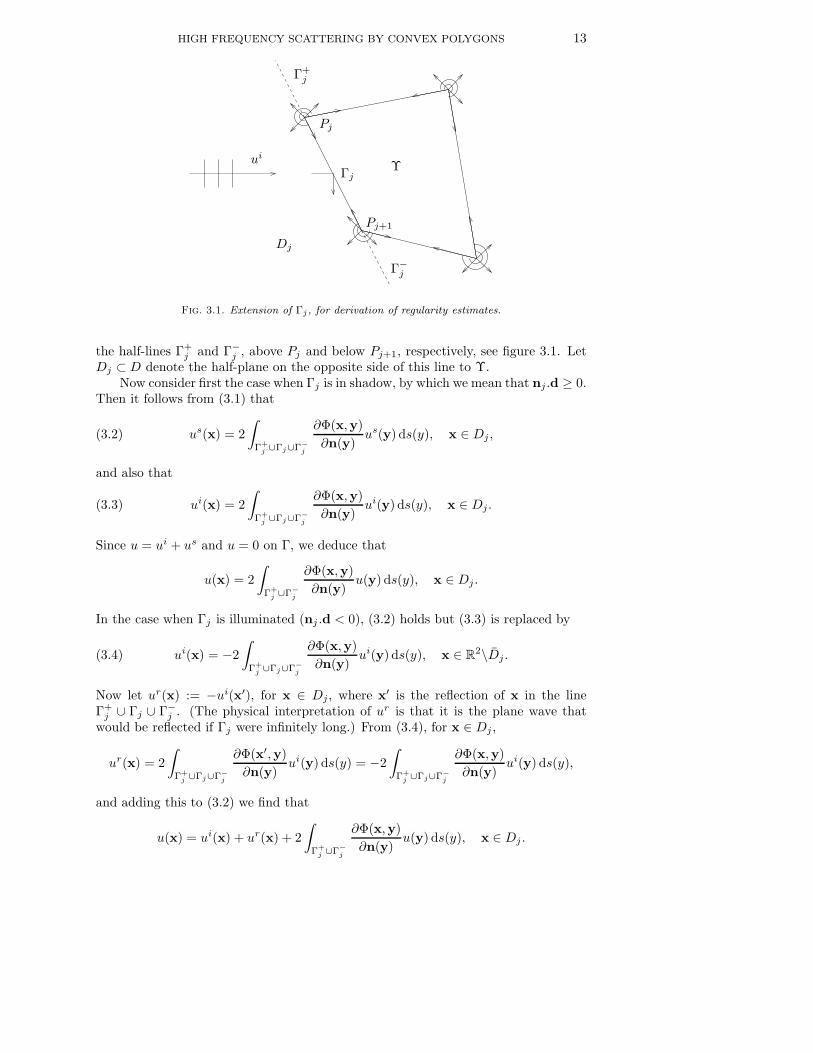
HIGH FREQUENCY SCATTERING BY CONVEX POLYGONS 13
ui
Pj
Pj+1
Υ
Dj
Γj
Γ+j
Γ−j
Fig. 3.1. Extension of Γj, for derivation of regularity estimates.
the half-lines Γ+j and Γ−
j , above Pj and below Pj+1, respectively, see figure 3.1. LetDj ⊂ D denote the half-plane on the opposite side of this line to Υ.
Now consider first the case when Γj is in shadow, by which we mean that nj .d ≥ 0.Then it follows from (3.1) that
us(x) = 2
∫
Γ+
j ∪Γj∪Γ−
j
∂Φ(x,y)
∂n(y)us(y) ds(y), x ∈ Dj ,(3.2)
and also that
ui(x) = 2
∫
Γ+
j ∪Γj∪Γ−
j
∂Φ(x,y)
∂n(y)ui(y) ds(y), x ∈ Dj .(3.3)
Since u = ui + us and u = 0 on Γ, we deduce that
u(x) = 2
∫
Γ+
j ∪Γ−
j
∂Φ(x,y)
∂n(y)u(y) ds(y), x ∈ Dj .
In the case when Γj is illuminated (nj .d < 0), (3.2) holds but (3.3) is replaced by
ui(x) = −2
∫
Γ+
j ∪Γj∪Γ−
j
∂Φ(x,y)
∂n(y)ui(y) ds(y), x ∈ R
2\Dj .(3.4)
Now let ur(x) := −ui(x′), for x ∈ Dj, where x′ is the reflection of x in the lineΓ+
j ∪ Γj ∪ Γ−j . (The physical interpretation of ur is that it is the plane wave that
would be reflected if Γj were infinitely long.) From (3.4), for x ∈ Dj ,
ur(x) = 2
∫
Γ+
j ∪Γj∪Γ−
j
∂Φ(x′,y)
∂n(y)ui(y) ds(y) = −2
∫
Γ+
j ∪Γj∪Γ−
j
∂Φ(x,y)
∂n(y)ui(y) ds(y),
and adding this to (3.2) we find that
u(x) = ui(x) + ur(x) + 2
∫
Γ+
j ∪Γ−
j
∂Φ(x,y)
∂n(y)u(y) ds(y), x ∈ Dj .

14 S. N. CHANDLER-WILDE AND S. LANGDON
Thus on an illuminated side it holds that
∂u
∂n(x) = 2
∂ui
∂n(x) + 2
∫
Γ+
j ∪Γ−
j
∂2Φ(x,y)
∂n(x)∂n(y)u(y) ds(y), x ∈ Γj .(3.5)
The same expression, but without the term 2∂ui
∂n(x), holds when Γj is in shadow. The
high frequency Kirchhoff or physical optics approximation to ∂u/∂n is just ∂u/∂n =2∂ui/∂n on the illuminated sides and zero on the sides in shadow. Thus the integral in(3.5) is an explicit expression for the correction to the physical optics approximation.
The representation (3.5) is very useful in understanding the oscillatory nature ofthe solution on a typical side Γj . In particular we note that, in physical terms, theintegral over Γ+
j can be interpreted as the normal derivative on Γj of the field due to
dipoles distributed along Γ+j . The point is that the field due to each dipole has the
same oscillatory behaviour eiks on Γj . To exhibit this explicitly, we calculate, usingstandard properties of Bessel functions [2], that, for x ∈ Γj , y ∈ Γ±
j , with x 6= y,
∂2Φ(x,y)
∂n(x)∂n(y)=
ikH(1)1 (k|x − y|)4|x − y| =
ik2
4eik|x−y|µ(k|x − y|),(3.6)
where µ(z) := e−izH(1)1 (z)/z, for z > 0. The function µ(z) is singular at z = 0 but
increasingly smooth as z → ∞, as quantified in the next theorem (cf. [19, lemma 2.5]).Theorem 3.1. For every ǫ > 0,
|µ(m)(z)| ≤ Cǫ(m+ 1)! z−3/2−m,
for z ≥ ǫ and m = 0, 1, . . ., where
Cǫ =2 4√
5(1 + ǫ−1/2)
π.(3.7)
Proof. From [51, equation (12.31)], µ(z) = (−2i/π)∫ ∞
0 (t2 − 2it)1/2e−zt dt, for
Rez > 0, where the branch of (t2 − 2it)1/2 is chosen so that Re(t2 − 2it)1/2 ≥ 0. Thus
µ(m)(z) = (−1)m+1 2i
π
∫ ∞
0
tm+1/2(t− 2i)1/2e−zt dt
and hence
|µ(m)(z)| ≤ 2
π
∫ ∞
0
tm+1/2(t2 + 4)1/4e−zt dt.
Now, for t ∈ [0, 1], (t2 + 4)1/4 ≤ 51/4 and, for t ∈ [1,∞), (t2 + 4)1/4 ≤ 51/4t1/2. So
π
2 4√
5|µ(m)(z)| ≤
∫ ∞
0
tm+1/2e−zt dt+
∫ ∞
0
tm+1e−zt dt
= Γ(m+3/2)z−3/2−m+Γ(m+2)z−2−m ≤ (1+ǫ−1/2)Γ(m+2)z−3/2−m,
for z ≥ ǫ.To make use of the above result, let x(s) denote the point on Γ whose arc-length
distance measured anticlockwise from P1 is s. Explicitly,
x(s) = Pj +(
s− Lj−1
)
(
Pj+1 − Pj
Lj
)
, for s ∈ [Lj−1, Lj], j = 1, . . . , n,
HIGH FREQUENCY SCATTERING BY CONVEX POLYGONS 15
where L0 := 0 and, for j = 1, . . . , n, Lj :=∑j
m=1 Lm is the arc-length distance fromP1 to Pj+1. Define
φ(s) :=1
k
∂u
∂n(x(s)), for s ∈ [0, L],(3.8)
where L := Ln, so that φ(s) is the unknown function of arc-length whose behaviourwe seek to determine. Let
Ψ(s) :=
2k
∂ui
∂n(x(s)), if s ∈ (Lns
, L)
0, if s ∈ (0, Lns),
so that Ψ(s) is the physical optics approximation to φ(s), and set ψj(s) := u(xj(s)),s ∈ R, where xj(s) ∈ Γ+
j ∪ Γj ∪ Γ−j is the point
xj(s) := Pj +(
s− Lj−1
)
(
Pj+1 − Pj
Lj
)
, −∞ < s <∞.
From (3.5) and (3.6) we have the explicit representation for φ on the side Γj , that
φ(s) = Ψ(s) +i
2[eiksv+
j (s) + e−iksv−j (s)], s ∈ [Lj−1, Lj], j = 1, . . . , n,(3.9)
where
v+j (s) := k
∫ Lj−1
−∞
µ(k|s− t|)e−iktψj(t) dt, s ∈ [Lj−1, Lj], j = 1, . . . , n,
v−j (s) := k
∫ ∞
Lj
µ(k|s− t|)eiktψj(t) dt, s ∈ [Lj−1, Lj], j = 1, . . . , n.
The terms eiksv+j (s) and e−iksv−j (s) in (3.9) are the integrals over Γ+
j and Γ−j , respec-
tively, in equation (3.5), and can be thought of as the contributions to ∂u/∂n on Γj
due to the diffracted rays travelling from Pj to Pj+1 and from Pj+1 to Pj , respectively,including all multiply diffracted ray components.
So the equation we wish to solve is (2.9), and we have the explicit representa-tion (3.9) for its solution. At first glance this may not appear to help us, since theunknown solution u appears (as ψj) on the right hand side of (3.9). However, (3.9)is extremely helpful in understanding how φ behaves since it explicitly separates outthe oscillatory part of the solution. The functions v±j are not oscillatory away fromthe corners, as the following theorem quantifies. In this theorem and hereafter we let
uM := supx∈D
|u(x)| <∞(3.10)
and note that ‖ψj‖∞ ≤ uM , j = 1, . . . , n.Theorem 3.2 (solution behaviour away from corners). For ǫ > 0, j = 1, . . . , n,
and m = 0, 1, . . ., it holds for s ∈ [Lj−1, Lj] that
|v+j
(m)(s)| ≤ 2Cǫm!uMkm(k(s− Lj−1))
−1/2−m, k(s− Lj−1) ≥ ǫ,
|v−j(m)
(s)| ≤ 2Cǫm!uMkm(k(Lj − s))−1/2−m, k(Lj − s) ≥ ǫ,
where Cǫ is given by (3.7).
16 S. N. CHANDLER-WILDE AND S. LANGDON
Proof. From theorem 3.1, for s ∈ [Lj−1 + ǫ/k, Lj],
|v+j
(m)(s)| = km+1
∣
∣
∣
∣
∣
∫ Lj−1
−∞
µ(m)(k|s− t|)e−iktψj(t) dt
∣
∣
∣
∣
∣
≤ Cǫ(m+ 1)!km+1‖ψj‖∞∫ Lj−1
−∞
(k|s− t|)−3/2−m dt
= Cǫ(m+ 1)!
(m+ 1/2)k−1/2‖ψj‖∞(s− Lj−1)
−1/2−m
≤ 2Cǫm!uMkm(k(s− Lj−1))−1/2−m.
The bound on v−j(m)
(s) is obtained similarly.The above theorem quantifies precisely the behaviour of ∂u/∂n away from the
corners. Complementing this bound, using theorem 2.3 we can study the behaviour of∂u/∂n near the corners. To state this result it is convenient to extend the definitionof φ from [0, L] to R by the periodicity condition φ(s+ L) = φ(s), s ∈ R.
Theorem 3.3 (solution behaviour near corners). If kRj = min(kLj−1, kLj) ≥π/4, for j = 1, . . . , n, then, for j = 1, . . . , n and 0 < k|s− Lj−1| ≤ π/12, it holds that
∣
∣
∣φ(m)(s)
∣
∣
∣≤ CuM
√
m+1
2m!km(k|s− Lj−1|)−αj−m, m = 0, 1, . . . ,
where
αj := 1 − π
Ωj∈ (0, 1/2)(3.11)
and C = 72√
2 π−1 e1/e+π/6.
Proof. To analyse the behaviour of u using (2.4) we will use the representationfor the Bessel function of order ν [2, (9.1.20)],
Jν(z)=2(z/2)ν
π1/2Γ(ν + 1/2)
∫ 1
0
(1 − t2)ν−1/2 cos(zt) dt, for Rez > 0, ν > −1/2,
where the branch of (z/2)ν is chosen so that (z/2)ν > 0 for z > 0 and (z/2)ν isanalytic in Rez > 0. This representation implies that
cos z ≤ Jν(z)π1/2Γ(ν + 1/2)
2(z/2)ν∫ 1
0 (1 − t2)ν−1/2 dt≤ 1, 0 ≤ z ≤ π/2.(3.12)
Recalling the definitions of R and G before theorem 2.3 and the definition (2.5) of thecoefficient an, we have that ρ := kR < π/2 and
|an| ≤2uM
Jnπ/Ωj(ρ)
.(3.13)
Thus, for 0 < r < R,
∣
∣anJnπ/Ωj(kr)
∣
∣ ≤ 2uM
cos ρ
( r
R
)nπ/Ωj
,(3.14)
HIGH FREQUENCY SCATTERING BY CONVEX POLYGONS 17
confirming that the series (2.4) converges for 0 ≤ r < R. Further, the bound (3.14)justifies differentiating (2.4) term by term to get that, for x ∈ Γj−1 ∩ G, ∂u
∂n(x) =
kF (kr), where
F (z) :=π
Ωjz
∞∑
n=1
nanJnπ/Ωj(z), Rez > 0, |z| < ρ.(3.15)
Since | cos z| ≤ e|Imz|, z ∈ C, so that | cos zt| ≤ e|Imz| for z ∈ C, 0 ≤ t ≤ 1, we seefrom (3.13) that, for Rez > 0,
∣
∣nanJnπ/Ωj(z)
∣
∣ ≤ 2uMn
cos ρe|Imz|
( |z|ρ
)nπ/Ωj
.(3.16)
So the series (3.15) is absolutely and uniformly convergent in Rez > 0, |z| < ρ0, forevery ρ0 < ρ, and F is analytic in Rez > 0, |z| < ρ. Further, from (3.16), and since,for 0 ≤ α < 1,
∑∞n=1 nα
n = α ddα
∑∞n=1 α
n = α(1−α)2 , we see that, for Rez > 0, |z| < ρ,
|F (z)| ≤ π
Ωj |z|2uM
cos ρ
e|Imz|
(1 − |z/ρ|π/Ωj)2
( |z|ρ
)π/Ωj
.
We can use this bound to obtain bounds on derivatives of F , and hence boundson derivatives of ∂u/∂n. For 0 < t ≤ ρ/3, 0 < ε < t, from Cauchy’s integral formulawe have that
|F (m)(t)| =m!
2π
∣
∣
∣
∣
∫
Γε
F (z)
(z − t)m+1dz
∣
∣
∣
∣
,
where Γε is the circle of radius ε centred on t, which lies in Rez > 0, |z| < ρ. Since
|F (z)| ≤ 2πuMe|Imz|(t− ε)π/Ωj−1
Ωjρπ/Ωj cos ρ(1 − (2/3)π/Ωj )2,
for z ∈ Γε, we see that
|F (m)(t)| ≤ 2πuMet(t− ε)π/Ωj−1ε−mm!
Ωjρπ/Ωj cos ρ(1 − (2/3)π/Ωj)2.(3.17)
Now, for α > 0, β > 0, (t−ε)−αε−β is minimised on (0, t) by the choice ε = βt/(α+β).Setting ε = mt/(m+ 1 − π/Ωj) in (3.17) we see that
|F (m)(t)| ≤ 2πuMetm!(m+ 1 − π/Ωj)m+1−π/Ωj tπ/Ωj−1−m
Ωjρπ/Ωj cos ρ(1 − (2/3)π/Ωj )2mm(1 − π/Ωj)1−π/Ωj.
Now
(m+ 1 − π/Ωj)m+1−π/Ωj
mm≤ (m+ 1/2)m+1/2
mm=
(
1+1
2m
)m√
m+1
2≤ e1/2
√
m+1
2,
2π
Ωj(1 − π/Ωj)1−π/Ωj (1 − (2/3)π/Ωj )2≤ 18
(1 − π/Ωj)1−π/Ωj≤ 18e1/e,
and hence
|F (m)(t)| ≤ 18e1/e+1/2+t√
m+ 1/2m!uM
ρπ/Ωj cos ρtπ/Ωj−1−m, 0 < t ≤ ρ/3.(3.18)

18 S. N. CHANDLER-WILDE AND S. LANGDON
Since ∂u∂n
(x) = kF (kr), this implies that
∣
∣
∣
∣
∂(m)
∂rm
[
∂u
∂n(x)
]∣
∣
∣
∣
≤ CuM km+1(kr)π/Ωj−1−m, 0 < r ≤ R/3 <π
6k,
where C = (18e1/e+1/2+π/6√
m+ 1/2m!)/(ρπ/Ωj cos ρ). Choosing ρ = π/4 the resultfollows.
From theorems 3.2 and 3.3, and equation (3.9), which gives that
v±j (s) = −2ie∓iks(φ(s) − Ψ(s)) − e±2iksv∓j (s),
we deduce the following corollary, in which αn+1 := α1.Corollary 3.4. Suppose that kRj = min(kLj−1, kLj) ≥ π/4, for j = 1, . . . , n.
Then, for m = 0, 1, . . ., there exists Cm > 0, dependent only on m, such that, ifj ∈ 1, . . . , n, then
|v+j
(m)(s)| ≤ CmuMkm(k(s− Lj−1))
−αj−m, 0 < k(s− Lj−1) ≤ π/12,
|v−j(m)
(s)| ≤ CmuMkm(k(Lj − s))−αj+1−m, 0 < k(Lj − s) ≤ π/12.
The following limiting case suggests that the bounds in theorem 3.2 and corollary3.4 are optimal in their dependence on k, s− Lj−1, and Lj − s, in the sense that nosharper bound holds uniformly in the angle of incidence. Suppose that Υ lies in theright hand half-plane with P1 located at the origin and d · n1 = 0, and consider thelimit min(kL0, kL1) → ∞ and Ω1 → 2π. In this limit α1 → 1/2 and it is plausible thatu(x) → uk.e.(x), where uk.e. is the solution to the following “knife edge” diffractionproblem: where Γk.e. := (x1, 0) : x1 ≥ 0, given the incident plane wave ui, find thetotal field uk.e. ∈ C2(R2 \ Γk.e.) ∩ C(R2) such that ∆uk.e. + k2uk.e. = 0 in R
2 \ Γk.e.,uk.e. = 0 on Γk.e., and uk.e. − ui has the correct radiating behaviour. The solutionto this problem which satisfies the physically correct radiation condition is given by[10, equation (8.24)]. This solution implies that ϕ(s) := 1
k∂uk.e.
∂n((s, 0)) = ±eiksv(s),
where the +/− sign is taken on the upper/lower surface of the knife edge and v(s) :=c(ks)−1/2, where c = e−iπ/4
√
2/π. The function v(s) and its derivatives satisfy thebounds on v+
1 in theorem 3.2 and corollary 3.4 (with αj = 1/2), but do not satisfy
any sharper bounds in terms of dependence on k or s− Lj−1.
4. The approximation space. Our aim now is to use the regularity resultsof §3 to design an optimal approximation space for the numerical solution of (2.9).We begin by rewriting (2.9) in parametric form. Defining, for j = 1, . . . , n,
aj :=pj+1 − pj
Lj, bj :=
qj+1 − qjLj
, cj := pj − ajLj−1, dj := qj − bjLj−1,
and noting that nj1 = bj , nj2 = −aj , we can rewrite (2.9) as
φ(s) +
∫ L
0
κ(s, t)φ(t) dt = f(s), s ∈ [0, L],(4.1)
where, for x(s) ∈ Γl, y(t) ∈ Γj , i.e. for s ∈ (Ll−1, Ll), t ∈ (Lj−1, Lj),
κ(s, t) := −1
2
[
ηH(1)0 (kR) + ik [(albj − blaj)t+ bl(cl − cj) − al(dl − dj)]
H(1)1 (kR)
R
]
,

HIGH FREQUENCY SCATTERING BY CONVEX POLYGONS 19
with R = R(s, t) :=√
(als− ajt+ cl − cj)2 + (bls− bjt+ dl − dj)2 and f ∈ L2(0, L)defined by
f(s) := 2i[bl sin θ + al cos θ + (η/k)]eik((als+cl) sin θ−(bls+dl) cos θ).
The first step in our numerical method is to separate off the explicitly knownleading order behaviour, the physical optics approximation Ψ(s). Thus we introducea new unknown,
ϕ := φ− Ψ ∈ L2(0, L).(4.2)
Substituting into (4.1) we have
ϕ+Kϕ = F,(4.3)
where the integral operator K : L2(0, L) → L2(0, L) and F ∈ L2(0, L) are defined by
Kψ(s) :=
∫ L
0
κ(s, t)ψ(t) dt, 0 ≤ s ≤ L, F := f − Ψ −KΨ.
Equation (4.3) is the integral equation we will solve numerically. By theorem 2.7,(4.3) has a unique solution in L2(0, L) and ‖(I +K)−1‖2 = CS , where CS is definedin (2.11) and I is the identity operator on L2(0, L).
We will design an approximation space to represent ϕ based on (3.9). The noveltyof the scheme we propose is that on each side Γj , j = 1, . . . , n, of the polygon, weapproximate v±j by conventional piecewise polynomials, rather than approximating
ϕ itself. This makes sense since, as quantified by theorem 3.2, the functions v±j aresmooth (their higher-order derivatives are small) away from the corners Pj and Pj+1.To approximate v±j we use piecewise polynomials of a fixed degree ν ≥ 0 on a gradedmesh, the mesh grading adapted in an optimal way to the bounds of theorems 3.2and 3.3. In [19] the 2D problem of scattering of a plane wave by a straight boundaryof piecewise constant surface impedance was considered. We will construct a similarmesh on each side of the polygon as was used on each interval of constant impedancein [19], except that we use a different grading near the corners, with the grading neareach corner dependent on the angle at that corner.
To construct this mesh we choose a constant c∗ > 0 (we take c∗ = 2π in thenumerical examples in §6) and set λ∗ := c∗/k. Next, for every A > λ∗, we define acomposite graded mesh on [0, A], with a polynomial grading on [0, λ∗] and a geometricgrading on [λ∗, A] (note that the mesh on [0, λ∗] is similar to that classically used nearcorners (e.g. [17], [7]) for solving Laplace’s equation on polygonal domains).
Definition 4.1. For A > λ∗, N = 2, 3, . . ., ΛN,A,q := y0, . . . , yN+NA,q is the
mesh consisting of the points
yi = λ∗(
i
N
)q
, i = 0, . . . , N, and yN+j := λ∗(
A
λ∗
)j/NA,q
, j = 1, . . . , NA,q,(4.4)
where NA,q := ⌈N∗⌉, i.e. NA,q is the smallest integer greater than or equal to N∗,and
N∗ :=− log(A/λ∗)
q log(1 − 1/N).

20 S. N. CHANDLER-WILDE AND S. LANGDON
Let us explain the rationale behind this definition. Having the bounds of theo-rems 3.2 and 3.3 in mind, the mesh on [0, λ∗] is chosen to be approximately optimal,if q is chosen appropriately (see theorem 4.2 below), in terms of equidistributing theerror between the subintervals of the mesh when s−α, with 0 < α < 1/2, is ap-proximated on [0, λ∗] in the L2 norm. That the mesh we propose on [0, λ∗] has thisproperty, and the appropriate choice of q as a function of α, are well-known and dateback to Rice [55]. Similarly, the mesh on [λ∗, A] is chosen to be approximately opti-mal, in terms of equidistributing the error between the subintervals of the mesh, whens−1/2 is approximated on [λ∗, A] in the L2 norm. Finally, the choice of N∗ ensures asmooth transition between the two parts of the mesh, and so approximately the sameL2 error in the two adjacent sub-intervals either side of λ∗. In particular, in the casethat NA,q = N∗, it holds that yN+1/yN = yN/yN−1, so that yN−1 and yN are pointsin both the polynomial and the geometric parts of the mesh. Note that, by the meanvalue theorem, − log(1 − 1/N) = 1/(ξN) for some ξ ∈ (1 − 1/N, 1), and hence
NA,q <N log(kA/c∗)
q+ 1.(4.5)
For a < b let ‖·‖2,(a,b) denote the norm on L2(a, b), ‖f‖2,(a,b) := ∫ b
a|f(s)|2ds1/2.
Similarly, for f ∈ C[a, b], let ‖f‖∞,(a,b) := supa<s<b |f(s)|. For A > λ∗, ν ∈ N ∪ 0,q ≥ 1, let ΠN,ν ⊂ L2(0, A) denote the set of piecewise polynomials
ΠN,ν := σ : σ|(yj−1,yj) is a polynomial of degree ≤ ν, for j = 1, . . . , N +NA,q,
and let P ∗N be the orthogonal projection operator from L2(0, A) to ΠN,ν, so that
setting p = P ∗Nf minimises ‖f − p‖2,(0,A) over all p ∈ ΠN,ν.
Theorem 4.2. Suppose that f ∈ C∞(0,∞), kA > c∗, and α ∈ (0, 1/2), and thatfor m = 0, 1, 2, . . . there exist constants cm > 0 such that
|f (m)(s)| ≤
cmkm(ks)−α−m, ks ≤ 1,
cmkm(ks)−1/2−m, ks ≥ 1.
(4.6)
Then, with the choice q := (2ν + 3)/(1 − 2α), there exists a constant Cν , dependentonly on c∗, ν, and α, such that, for N = 2, 3, . . .,
‖f − P ∗Nf‖2,(0,A) ≤
Cν cν(1 + log(kA/c∗))1/2
k1/2Nν+1,
where cν := max(c0, cν+1).
Proof. Throughout the proof let Cν denote a positive constant whose value de-pends on ν, c∗, and α, not necessarily the same at each occurrence. For 0 ≤ a < b ≤ A,let pa,b,ν denote the polynomial of degree ≤ ν which is the best approximation to fin the L2 norm on (a, b). Then it follows from Taylor’s theorem that
‖f − pa,b,ν‖2,(a,b) ≤ Cν(b− a)ν+3/2‖f (ν+1)‖∞,(a,b).(4.7)
Now
‖f − P ∗Nf‖2
2,(0,A) =
N+NA,q∑
j=1
∫ yj
yj−1
|f − P ∗Nf |2 ds =
N+NA,q∑
j=1
ej ,(4.8)

HIGH FREQUENCY SCATTERING BY CONVEX POLYGONS 21
where ej := ‖f − pyj−1,yj,ν‖22,(yj−1,yj)
. From the definition (4.4) we see that
e1 ≤∫ y1
0
|f(s)|2 ds ≤ c20k−2α
∫ λ∗/Nq
0
s−2α ds ≤ Cνc20
kN2ν+3.(4.9)
Using (4.7) we have, for j = 2, 3, . . . , N +NA,q,
ej ≤ Cν(yj − yj−1)2ν+3‖f (ν+1)‖2
∞,(yj−1,yj).(4.10)
Further, for j = 2, . . . , N ,
yj − yj−1 =c∗
kN q[jq − (j − 1)q] ≤ c∗qjq−1
kN q,(4.11)
and, using (4.6) and since N/(j − 1) ≤ 2N/j,
‖f (ν+1)‖∞,(yj−1,yj) ≤ cν+1k−αy−α−ν−1
j−1 ≤ cν+1kν+1
(
2N
j
)q(α+ν+1)
.(4.12)
Combining (4.10)-(4.12) we see that, for j = 2, . . . , N ,
ej ≤ Cνc2ν+1
kN2ν+3.(4.13)
For j = N + 1, . . . , NA,q, recalling (4.4) and the choice of N∗, and then using (4.11),
yj − yj−1 = yj−1
(
yj − yj−1
yj−1
)
≤ yj−1
(
yN − yN−1
yN−1
)
≤ yj−1q
N − 1≤ 2yj−1
q
N.
Also, from (4.6),
‖f (ν+1)‖∞,(yj−1,yj) ≤ cν+1k−1/2y
−ν−3/2j−1 .
Using these bounds in (4.10), we see that the bound (4.13) holds also for j = N +1, . . . , N +NA,q. Combining (4.8), (4.9), and (4.13),
‖f − P ∗Nf‖2
2,(0,A) ≤Cν c
2ν(N +NA,q)
kN2ν+3≤ Cν c
2ν(1 + log(kA/c∗))
kN2ν+2,
using (4.5). Hence the result follows.We assume through the remainder of the paper that c∗ > 0 is chosen so that
kLj ≥ c∗, j = 1, . . . , n.(4.14)
For j = 1, . . . , n, recalling (3.11), we define qj := (2ν + 3)/(1 − 2αj), and the twomeshes
Γ+j := Lj−1 + ΛN,Lj,qj
, Γ−j := Lj − ΛN,Lj,qj+1
.
Letting e±(s) := e±iks, s ∈ [0, L], we then define
VΓ+
j ,ν := σe+ : σ ∈ ΠΓ+
j ,ν, VΓ−
j ,ν := σe− : σ ∈ ΠΓ−
j ,ν,

22 S. N. CHANDLER-WILDE AND S. LANGDON
for j = 1, . . . , n, where
ΠΓ+
j ,ν := σ ∈ L2(0, L) : σ|(Lj−1+ym−1,Lj−1+ym) is a polynomial of degree ≤ ν,
for m = 1, . . . , N +NLj,qj, and σ|(0,Lj−1)∪(Lj,L) = 0,
ΠΓ−
j ,ν := σ ∈ L2(0, L) : σ|(Lj−ym,Lj−ym−1)is a polynomial of degree ≤ ν,
for m = 1, . . . , N +NLj,qj+1, and σ|(0,Lj−1)∪(Lj,L) = 0,
with 0 = y0 < y1 < . . . < yN+NLj,qj= Lj the points of the mesh ΛN,Lj,qj
, and
0 = y0 < y1 < . . . < yN+NLj,qj+1= Lj the points of the mesh ΛN,Lj,qj+1
. We define
P+N and P−
N to be the orthogonal projection operators from L2(0, L) onto ΠΓ+,ν andΠΓ−,ν , respectively, where ΠΓ±,ν denotes the linear span of
⋃
j=1,...,n ΠΓ±
j ,ν . We also
define the functions v± ∈ L2(0, L) by
v+(s) := v+j (s), v−(s) := v−j (s), Lj−1 < s < Lj, j = 1, . . . , n.
We then have the following error estimate, in which uM is as defined in (3.10) and weabbreviate ‖ · ‖2,(0,L) by ‖ · ‖2.
Theorem 4.3. There exists a constant Cν > 0, dependent only on c∗, ν, and Ω1,Ω2, . . . , Ωn, such that
‖v+ − P+N v+‖2 ≤ CνuM
n1/2(1 + log(kL/c∗))1/2
k1/2Nν+1,
where L := (L1 . . . Ln)1/n, with an identical bound holding on ‖v− − P−N v−‖2.
Proof. From theorem 3.2, corollary 3.4, and theorem 4.2,
‖v+ − P+N v+‖2
2 =
n∑
j=1
‖v+j − P+
N v+j ‖2
2,(Lj−1,Lj)≤ n
C2νu
2M (1 + log(kL))
kN2ν+2,
and the result follows.Our approximation space VΓ,ν is the linear span of
⋃
j=1,...,n
VΓ+
j ,ν ∪ VΓ−
j ,ν.
The dimension of this approximation space, i.e. the number of degrees of freedom, is
MN = 2(ν + 1)
n∑
j=1
(N +NLj,qj) < 2(ν + 1)nN(1 +N−1 + log(kL/c∗))(4.15)
by (4.5). We define PN to be the operator of orthogonal projection from L2(0, L)onto VΓ,ν . It remains to prove a bound on ‖ϕ− PNϕ‖2, showing that our mesh andapproximation space are well adapted to approximating ϕ.
To use theorem 4.3 we note from (3.9) and (4.2) that ϕ = i2 (e+v+ + e−v−). But
e+P+N v+ +e−P
−N v− ∈ VΓ,ν and PNϕ is the best approximation to ϕ in VΓ,ν . Applying
theorem 4.3 we thus have that
‖ϕ− PNϕ‖2 ≤ ‖ϕ− i
2(e+P
+N v+ + e−P
−N v−)‖2
=1
2‖e+(v+ − P+
N v+) + e−(v− − P−N )‖2
≤ ‖e+‖∞‖v+ − P+N v+‖2 + ‖e−‖∞‖v− − P−
N v−‖2
≤ CνuMn1/2(1 + log1/2(kL))
k1/2Nν+1.

HIGH FREQUENCY SCATTERING BY CONVEX POLYGONS 23
Combining this bound with (4.15) we obtain the following main result of the paper.We remind the reader that we are assuming throughout that (4.14) holds.
Theorem 4.4. There exist positive constants Cν and C′ν , depending only on c∗,
ν, and Ω1, Ω2, . . . , Ωn, such that
k1/2‖ϕ− PNϕ‖2 ≤ CνuMn1/2(1 + log(kL/c∗))1/2
Nν+1≤ C′
νuM(n[1 + log(kL/c∗)])ν+3/2
Mν+1N
.
A comment on the factor k1/2 on the left hand side is probably helpful. Reflectingthat the solution of the physical problem must be independent of the unit of lengthmeasurement and that we are designing our numerical scheme to preserve this prop-erty, it is easy to see that the values of both k1/2‖ϕ‖2 and k1/2‖ϕ − PNϕ‖2 remainfixed as k changes, if we keep kLj fixed for j = 1, . . . , n (and also, of course, keepΩj , j = 1, . . . , n, c∗, and ν fixed). Thus inclusion of the factor k1/2 ensures that thevalue of k1/2‖ϕ−PNϕ‖2 is independent of the unit of length measurement as are thebounds on the right hand side.
5. Galerkin method. Theorem 4.4 has shown that it is possible to approximateaccurately the solution of the integral equation (4.3) with a number of degrees of free-dom that grows only very modestly as the wave number increases. To select an approx-imation, ϕN , from the approximation space VΓ,ν we use the Galerkin method. Let (·, ·)denote the usual inner product on L2(0, L), defined by (χ1, χ2) :=
∫ L
0 χ1(s)χ2(s) ds,
so that ‖χ‖2 = (χ, χ)1/2. Then our Galerkin method approximation ϕN ∈ VΓ,ν isdefined by
(ϕN , ρ) + (KϕN , ρ) = (F, ρ), for all ρ ∈ VΓ,ν ;(5.1)
equivalently
ϕN + PNKϕN = PNF.(5.2)
Our goal now is to show that (5.2) has a unique solution ϕN , to establish a boundon the error ‖ϕ−ϕN‖2 in this numerical method, and to relate this error to the bestapproximation error ‖ϕ−PNϕ‖2. We begin by establishing that I+PNK is invertibleif N is large enough. We remind the reader (see the end of §2) that we are assumingthat η ∈ R, the coupling parameter in the integral equation, is chosen with η 6= 0which ensures that I +K is invertible.
Theorem 5.1. For all v ∈ L2(0, L), ‖PNv − v‖2 → 0 as N → ∞.Proof. Since ‖PN‖2 = 1 it is enough to show that PNv → v in L2(0, L) for all
v ∈ C∞[0, L], a dense subset of L2(0, L). But this follows from theorem 4.2 and thedefinition of PN .
Theorem 5.2. There exists a constant N∗ ≥ 2, dependent only on Γ, k, and η,such that, for N ≥ N∗, the operator I + PNK : L2(0, L) → L2(0, L) is bijective with
Cs := supN≥N∗
‖(I + PNK)−1‖2 <∞,(5.3)
so that (5.2) has exactly one solution for N ≥ N∗.Proof. Recalling the discussion at the end of §2, we note that it holds that
K = K1 + K2, where ‖K1‖2 < 1 and K2 is a compact operator on L2(0, L). Since‖PNK1‖2 ≤ ‖K1‖2 < 1, I+PNK1 is invertible and ‖(I+PNK1)
−1‖2 ≤ (1−‖K1‖2)−1.

24 S. N. CHANDLER-WILDE AND S. LANGDON
Since K2 is compact and I +K is injective, it follows from theorem 5.1 and standardperturbation arguments for projection methods (e.g. [7, theorem 8.2.1], [17]) that(I + PNK)−1 exists and is uniformly bounded for all N sufficiently large.
From (4.3) and (5.2) it follows that ϕ−ϕN = (I+PNK)−1(ϕ−PNϕ), and hence
‖ϕ− ϕN‖2 ≤ ‖(I + PNK)−1‖2‖ϕ− PNϕ‖2.(5.4)
Combining (5.3) and (5.4) with theorem 4.4 we obtain our final error estimate.Theorem 5.3. There exist positive constants Cν and C′
ν , depending only on c∗,ν, and Ω1, Ω2, . . . , Ωn, such that
k1/2‖ϕ− ϕN‖2 ≤ CsCνuMn1/2(1 + log(kL/c∗))1/2
Nν+1
≤ CsC′νuM
(n[1 + log(kL/c∗)])ν+3/2
Mν+1N
,(5.5)
for N ≥ N∗, where N∗ and Cs are as defined in theorem 5.2.Note that we will take c∗ = 2π and η = k in all our numerical calculations
in the next section. Note also that, while the constants Cν and C′ν , from the best
approximation theorem 4.4, depend only on c∗, ν and the corner angles of Γ, thenumbers N∗ and Cs depend additionally on k, L1, L2, . . . , Ln and η. We do notattempt the difficult task of elucidating this dependence in this paper. We note onlythat, very recently, for the boundary integral equation formulation (2.9) applied toscattering by a circle, Dominguez et al. [28] have shown that I + K is elliptic ifη = ±k and k is sufficiently large, so that every Galerkin method is automaticallystable; specifically, (5.3) holds for every N∗ if PN is the orthogonal projection fromL2(0, L) onto the Galerkin approximation space. Further it follows from results in [28]that, at worst, Cs = O(k1/3) as k → ∞ in the circle case. Our numerical results in§6 will suggest the stronger result that, for our particular scheme and geometry, thebound of theorem 5.3 holds with a constant Cs independent of k. We recall from §2(equation (2.12)) that it has been shown that the corresponding continuous continuityconstant CS = O(1) as k → ∞ if the choice η = k is made.
Of course our aim in approximating ϕ by ϕN is to approximate ∂+n u and hence,
via (2.7), the solution u of the scattering problem. Clearly, from (3.8) and (4.2), anapproximation to ∂u/∂n is
∂u
∂n(x(s)) ≈ k(Ψ(s) + ϕN (s)), 0 ≤ s ≤ L.
Using this approximation in (2.7), we conclude that
u(x) ≈ uN (x) := ui(x) − k
∫ L
0
Φ(x,x(s))[Ψ(s) + ϕN (s)] ds, x ∈ D.(5.6)
Theorem 5.3 implies the following error estimate.Theorem 5.4. There exist positive constants Cν and C′
ν , depending only on c∗,ν, and Ω1, Ω2, . . . , Ωn, such that
supx∈D |u(x) − uN(x)|supx∈D |u(x)| ≤ CsCν
n(1 + log(kL/c∗))
Nν+1≤ CsC
′ν
(n[1 + log(kL/c∗]))ν+2
Mν+1N
,
for N ≥ N∗, where N∗ and Cs are as defined in theorem 5.2.
HIGH FREQUENCY SCATTERING BY CONVEX POLYGONS 25
Proof. From (2.7) and (5.6),
|u(x) − uN(x)| = k
∣
∣
∣
∣
∣
∫ L
0
Φ(x,x(s)) [ϕ(s) − ϕN (s)] ds
∣
∣
∣
∣
∣
≤ k
4
∫ L
0
|H(1)0 (k|x − x(s)|)|2 ds
1/2
‖ϕ− ϕN‖2
≤ k
4
2n
∑
j=1
∫ Lj/2
0
|H(1)0 (kt)|2 dt
1/2
‖ϕ− ϕN‖2
≤ Cνk1/2n1/2(1 + log(kL/c∗))1/2‖ϕ− ϕN‖2,
where we have used that |H(1)0 (t)| is a monotonic decreasing function of t on (0,∞)
and that |H(1)0 (t)| = O(t−1/2) as t → ∞ (see e.g. [2]). The result now follows from
theorem 5.3.
6. Numerical results. There has been much work on the optimal choice of theparameter η in (2.9) (see e.g. [3, 43]). Here we choose η = k as in [28]. We alsoset c∗ = 2π and restrict attention to the case ν = 0. For higher values of ν theimplementation of the scheme is similar. Note that, with c∗ = 2π and ν = 0, thereare approximately N degrees of freedom used to represent the solution in the firstwavelength on each side adjacent to a corner.
The equation we wish to solve is (5.1) with ν = 0. Writing ϕN as a linearcombination of the basis functions of VΓ,0, we have
ϕN (s) =
MN∑
j=1
vjρj(s), 0 ≤ s ≤ L,
where ρj is the jth basis function and MN is the dimension of VΓ,0. For p = 1, . . . , n,where n is the number of sides of the polygon, we define n±
p to be the number ofpoints in the mesh Γ±
p , so n+p = N +NLp,qp
, n−p = N +NLp,qp+1
, and we denote the
points of the mesh Γ±p by s±p,l, for l = 1, . . . , n±
p , with s±p,1 < . . . < s±p,n±
p
. Setting
n1 := 0, np :=∑p−1
j=1(n+j + n−
j ), for p = 2, . . . , n− 1, we define, for p = 1, . . . , n,
ρnp+j(s) :=
eiksχ(s+
p,j−1,s+
p,j)(s)/
√
s+p,j − s+p,j−1, j = 1, . . . , n+p ,
e−iksχ(s−
p,j−1,s−
p,j)(s)/
√
s−p,j − s−p,j−1, j = n+p + 1, . . . , n+
p + n−p ,
where χ(y1,y2) denotes the characteristic function of the interval (y1, y2). From (4.15),
MN =∑n
j=1(n+j + n−
j ) < 2nN(3/2 + log(kL/c∗)).Equation (5.1) with ν = 0 is equivalent to the linear system
MN∑
j=1
vj((ρj , ρm) + (Kρj, ρm)) = (F, ρm), m = 1, . . . ,MN .(6.1)
In order to set up this linear system we need to determine the integrals (ρj , ρm),(Kρj , ρm) and (F, ρm). We note that many of the integrals (Kρj , ρm) and (F, ρm)are highly oscillatory, in particular all these integrals become highly oscillatory in the

26 S. N. CHANDLER-WILDE AND S. LANGDON
limit as k → ∞ with N fixed. The efficient calculation of these integrals is an aspectof the numerical scheme which requires further research, as discussed in §1.2. Butnote that explicit formulae for the analytic evaluation of some of these integrals, anda consideration of the quadrature techniques required to evaluate the rest of themnumerically, are presented in [44].
Another important issue is the conditioning of the linear system. Standard anal-ysis of the Galerkin method for second kind equations [7] implies that, where M :=[(ρj , ρm)] is the mass matrix (which is necessarily Hermitian and positive definite) andA = [(ρj , ρm) + (Kρj, ρm)] is the whole matrix, it holds that cond2A ≤ Cscond2M ,where Cs is defined by (5.3). Thus theorem 5.2 implies that cond2A is bounded asN → ∞ if the mass matrix is well-conditioned. Unfortunately, it appears that, asN → ∞ with k fixed, M must ultimately become badly conditioned. However, theresults below will show only moderate condition numbers of A even for large values ofN (see table 6.1). More positively, in the limit as k → ∞ with N fixed, cond2M → 1.To see this we observe that, if (ρj , ρm) is a non-zero off-diagonal element of the massmatrix (in which case the supports of ρj and ρm are overlapping subintervals of the
meshes Γ+p and Γ−
p , for some side p), it holds that |(ρj , ρm)| = | sin(ko)|√
o/(kS1S2),where S1 and S2 are the lengths of the two-subintervals, o the length of the overlap.
As a numerical example, we consider the problem of scattering by a square withsides of length 2π. In this case n = 4 and Ωj = 3π/2, j = 1, 2, 3, 4. The corners of thesquare are P1 := (0, 0), P2 := (2π, 0), P3 := (2π, 2π), P4 := (0, 2π), and the incidentangle is θ = π/4, so the incident field is directed towards P4, with P2 in shadow (asshown in figure 6.1, where the total acoustic field is plotted for k = 10).
Fig. 6.1. Total acoustic field, scattering by a square, k = 10. Incident field is directed from thetop left corner towards the bottom right corner.
In figure 6.2 we plot |ϕN (s)| against s for k = 10 and N = 4, 16, 64, 256. As weexpect, |ϕN (s)| is highly peaked at the corners of the polygon, s = 0, 2π, 4π, 6πand 8π (which is the same corner as s = 0), where ϕ(s) is infinite. Except at these

HIGH FREQUENCY SCATTERING BY CONVEX POLYGONS 27
corners, |ϕN (s)| appears to be converging pointwise as N increases. (We do not plotϕN (s) itself which is highly oscillatory.)
−0.5 0 0.5 1 1.5 2 2.5 3 3.5 4 4.510
−3
10−2
10−1
100
101
102
103
N=4N=16N=64N=256
s/2π
|ϕN
(s)|
Fig. 6.2. |ϕN (s)| plotted against s, various N , for scattering by a square of side length tenwavelengths.
In order to test the convergence of our scheme, we take the “exact” solution to bethat computed with a large number of degrees of freedom, namely with N = 256. Fork = 5 and k = 320 the relative L2 errors ‖ϕN −ϕ256‖2/‖ϕ256‖2 are shown in table 6.1(all L2 norms are computed by approximating by discrete L2 norms, sampling at100000 evenly spaced points around the boundary of the square). For this example,
k N MN k1/2‖ϕN − ϕ256‖2 ‖ϕN − ϕ256‖2/‖ϕ256‖2 EOC cond2A5 8 88 5.7339×10⁻¹ 2.4426×10⁻¹ 9.5×100
16 176 3.7454×10⁻¹ 1.5955×10⁻¹ 0.6 4.6×101
32 360 1.6176×10⁻¹ 6.8909×10⁻² 0.9 2.6×101
64 712 7.7267×10⁻² 3.2916×10⁻² 1.0 2.4×10²
128 1416 3.3541×10⁻² 1.4289×10⁻² 1.0 1.5×10³
320 8 120 7.0765×10⁻¹ 3.6736×10⁻¹ 2.4×10²
16 240 5.9792×10⁻¹ 3.1040×10⁻¹ 0.2 6.9×10²
32 472 1.9668×10⁻¹ 1.0211×10⁻¹ 0.9 8.1×10²
64 944 7.5808×10⁻² 3.9354×10⁻² 1.1 1.1×10³
128 1888 4.8814×10⁻² 2.5341×10⁻² 1.0 3.8×10³
Table 6.1Errors and relative L2 errors, various N , k = 5 and k = 320.
theorem 5.3 predicts that, for N ≥ N∗, ‖ϕ− ϕN‖2 ≤ CN−1, where C is a constant.Thus theorem 5.3 predicts that, for N > N∗, the average rate of convergence,
EOC :=log(‖ϕ− ϕN‖2/‖ϕ− ϕN∗‖2)
log(N/N∗)≥ 1 − C
log(N/N∗)∼ 1

28 S. N. CHANDLER-WILDE AND S. LANGDON
as N → ∞, where C := log(‖ϕ−ϕN‖2/C). This behaviour is clearly seen in the EOCvalues (defined with N∗ = 8) in table 6.1, for both values of k. We also show in ta-ble 6.1 the 2-norm condition number, cond2A, of the matrix A = [(ρj , ρm)+(Kρj, ρm)]for each example. Unlike methods where the approximation space is formed by mul-tiplying standard finite element basis functions by many plane waves, travelling in alarge number of directions [27, 53, 37], the condition number does not grow signifi-cantly as the number of degrees of freedom increases.
In table 6.2 we fix N = 64 and show ‖ϕ64 − ϕ256‖2/‖ϕ256‖2 and k1/2‖ϕ64 −ϕ256‖2 for increasing values of k. Both measures of errors remain approximatelyconstant in magnitude as k increases. Recall that, keeping N fixed as k increasescorresponds to keeping the number of degrees of freedom per wavelength fixed neareach corner and increasing the total number of degrees of freedom, MN , approximatelyin proportion to log(kL). Thus these results are consistent with the approximationerror estimate of theorem 4.2 which suggests that increasing MN proportional tolog3/2(kL) is enough to keep the error bounded; indeed these results are suggestivethat the bound (5.5) in the Galerkin error estimate, theorem 5.3, holds with a constantCs which is independent of k. Note that the condition number of the coefficient matrixA only increases modestly as k increases, and is approximately constant for k ≥ 40.
k MN k1/2‖ϕ64 − ϕ256‖2 ‖ϕ64 − ϕ256‖2/‖ϕ256‖2 cond2A5 712 7.7267×10⁻² 3.2916×10⁻² 2.4×10²
10 752 6.6373×10⁻² 2.8702×10⁻² 8.4×101
20 792 3.8309×10⁻¹ 1.6914×10⁻¹ 5.1×10³
40 824 1.3162×10⁻¹ 5.9856×10⁻² 1.2×10³
80 864 7.4315×10⁻² 3.4801×10⁻² 2.7×10³
160 904 7.0884×10⁻² 3.4570×10⁻² 1.4×10³
320 944 7.5808×10⁻² 3.9354×10⁻² 1.1×10³
640 984 6.4280×10⁻² 3.5693×10⁻² 1.5×10³
Table 6.2Errors and relative L2 errors, various k, N = 64.
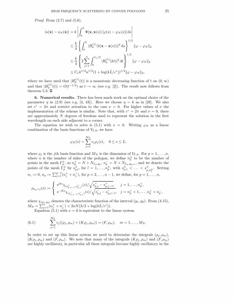
In table 6.3 we show numerical convergence of the total field uN(x) at the threepoints x = (−π, 3π) (illuminated), x = (3π, 3π), and x = (3π,−π) (shadow), fork = 5 and k = 320. The errors are consistent with the estimate of theorem 5.4. Asmight be expected for the computation of linear functionals of ϕN , the relative errorsin table 6.3 are a lot smaller and converge to zero more rapidly than the relative errorsin the computation of the boundary data in tables 6.1 and 6.2.
7. Conclusions. In this paper we have described a novel Galerkin boundaryintegral equation method for solving problems of high frequency scattering by convexpolygons. In §2, building on previous results for Lipschitz domains [56, 48, 50, 49], wehave shown that the standard second kind boundary integral equations for the exteriorDirichlet problem for the Helmholtz equation are well-posed for general Lipschitzdomains in a scale of Sobolev spaces. We have understood very completely in §3the oscillatory behaviour of the normal derivative of the field on the boundary of thepolygon. We have then used this understanding to design an optimal graded meshfor approximation of the diffracted field by products of piecewise polynomials andplane waves. Our error analysis demonstrates that the number of degrees of freedomrequired to achieve a prescribed level of accuracy using the best approximation tothe solution from the approximation space grows only logarithmically with respect
HIGH FREQUENCY SCATTERING BY CONVEX POLYGONS 29
k N x = (−π, 3π) x = (3π, 3π) x = (3π,−π)5 4 1.9587×10⁻² 1.0071×10⁻³ 1.5885×10⁻²
8 4.2629×10⁻³ 2.8031×10⁻³ 2.3215×10⁻³
16 3.6284×10⁻⁴ 3.1410×10⁻⁴ 1.3513×10⁻³
32 6.7523×10⁻⁵ 2.9803×10⁻⁵ 1.7939×10⁻⁵
64 1.2675×10⁻⁵ 5.9626×10⁻⁶ 4.6158×10⁻⁶
320 4 2.2938×10⁻³ 2.9350×10⁻³ 2.0897×10⁻²
8 4.3176×10⁻³ 1.5157×10⁻³ 1.1652×10⁻²
16 3.3908×10⁻³ 9.6409×10⁻⁴ 9.3922×10⁻³
32 3.3898×10⁻⁴ 1.6984×10⁻⁴ 9.0526×10⁻⁴
64 1.0022×10⁻⁴ 9.6493×10⁻⁵ 2.6204×10⁻⁴
Table 6.3Relative errors, |uN (x) − u256(x)|/|u256(x)|, as a function of N , at three points x.
to the wave number k as k → ∞. Numerical experiments indicate that the samestatement holds for the Galerkin approximation from the same approximation space.However, while we have established that the error in the Galerkin approximationspace is bounded by the stability constant Cs times the best approximation error,our theorem 5.3 only holds for a sufficiently refined mesh and we have not establisheda bound on Cs which is independent of k, to mirror the recently established bound(2.12) on the corresponding continuous stability constant.
There are very many open problems in extending the results of this paper to moregeneral scatterers. In this extension we expect that our mesh design and parts of ouranalysis will have relevance for representing certain components of the total field. Forexample, in the case of 2D convex curvilinear polygons, something close to the meshgrading we use may be appropriate on each side of the polygon, especially at higherfrequencies when the waves diffracted by the corners become more localised near thecorners. In the case of three-dimensional scattering by convex polyhedra it seemsto us that the mesh we propose may be useful in representing the variation of edgescattered waves in the direction perpendicular to the edge.
Acknowledgement The authors gratefully acknowledge helpful discussions withMarkus Melenk (Vienna) and Johannes Elschner (WIAS, Berlin) and the helpfulcomments of the anonymous referees.
REFERENCES
[1] T. Abboud, J. C. Nedelec, and B. Zhou, Methodes des equations integrales pour les hautesfrequences, C.R. Acad. Sci. I-Math, 318 (1994), pp. 165–170.
[2] M. Abramowitz and I. Stegun, Handbook of Mathematical Functions, Dover, 1972.[3] S. Amini, On the choice of the coupling parameter in boundary integral formulations of the
exterior acoustic problem, Applicable Analysis, 35 (1990), pp. 75–92.[4] S. Amini and N. D. Maines, Preconditioned Krylov subspace methods for boundary element
solution of the Helmholtz equation, Internat. J. Numer. Methods Engrg., 41 (1998), pp. 875–898.
[5] S. Amini and A. T. J. Profit, Multi-level fast multipole Galerkin method for the boundaryintegral solution of the exterior Helmholtz equation, in Current trends in scientific comput-ing (Xi’an, 2002), vol. 329 of Contemp. Math., Amer. Math. Soc., Providence, RI, 2003,pp. 13–19.
[6] S. Arden, S. N. Chandler-Wilde, and S. Langdon, A collocation method for high frequencyscattering by convex polygons, J. Comp. Appl. Math., (2006). Published online, July 2006,doi:10.1016/j.cam.2006.03.028.

30 S. N. CHANDLER-WILDE AND S. LANGDON
[7] K. E. Atkinson, The numerical solution of integral equations of the second kind, CambridgeUniversity Press, 1997.
[8] I. Babuska and J. M. Melenk, The partition of unity method, Int. J. Numer. Meth. Eng., 40(1997), pp. 727–758.
[9] I. Babuska and S. Sauter, Is the pollution effect of the FEM avoidable for the Helmholtzequation considering high wave numbers, SIAM J. Numer. Anal., 34 (1997), pp. 2392–2423. Reprinted in SIAM Rev. 42 (3), 451-484, 2000.
[10] J. J. Bowman, T. B. A. Senior, and P. L. E. Uslenghi, Electromagnetic and AcousticScattering by Simple Shapes, North-Holland, Amsterdam, 1969.
[11] H. Brakhage and P. Werner, Uber das Dirichletsche Aussenraumproblem fur dieHelmholtzsche Schwingungsgleichung, Arch. Math., 16 (1965), pp. 325–329.
[12] O. P. Bruno, C. A. Geuzaine, J. A. Monro Jr, and F. Reitich, Prescribed error toleranceswithin fixed computational times for scattering problems of arbitrarily high frequency: theconvex case, Phil. Trans. R. Soc. Lond A, 362 (2004), pp. 629–645.
[13] O. P. Bruno and L. A. Kunyansky, A fast, high-order algorithm for the solution of surfacescattering problems: Basic implementation, tests and applications, J. Comput. Phys., 169(2001), pp. 80–110.
[14] A. Buffa and S. Sauter, On the acoustic single layer potential: stabilization and Fourieranalysis, SIAM J. Sci. Comput. To appear.
[15] A. J. Burton and G. F. Miller, The application of integral equation methods to the numericalsolution of some exterior boundary-value problems, Proc. R. Soc. Lond. A, 323 (1971),pp. 201–210.
[16] O. Cessenat and B. Despres, Using plane waves as base functions for solving time har-monic equations with the ultra weak variational formulation, J. Comp. Acoust., 11 (2003),pp. 227–238.
[17] G. Chandler, Galerkin’s method for boundary integral equations on polygonal domains, J.Austral. Math. Soc., Series B, 26 (1984), pp. 1–13.
[18] S. N. Chandler-Wilde, Boundary value problems for the Helmholtz equation in a half-line,in Proc. 3rd Int. Conf. on Mathematical and Numerical Aspects of Wave Propagation,G. Cohen, ed., SIAM, Philadelphia, 1995.
[19] S. N. Chandler-Wilde, S. Langdon, and L. Ritter, A high-wavenumber boundary-elementmethod for an acoustic scattering problem, Phil. Trans. R. Soc. Lond. A, 362 (2004),pp. 647–671.
[20] S. N. Chandler-Wilde and P. Monk, Wave-number-explicit bounds in time-harmonic scat-tering. Submitted for publication., 2006.
[21] W. C. Chew, J. M. Song, T. J. Cui, S. Velamparambil, M. L. Hastriter, and B. Hu,Review of large scale computing in electromagnetics with fast integral equation solvers,CMES-Computer Modeling Engineering Sciences, 5 (2004), pp. 361–372.
[22] S. H. Christiansen and J. C. Nedelec, Preconditioners for the numerical solution of bound-ary integral equations from electromagnetism, C.R. Acad. Sci. I-Math, 331 (2000), pp. 733–738.
[23] D. Colton and R. Kress, Integral Equation Methods in Scattering Theory, Wiley, 1983.[24] , Inverse Acoustic and Electromagnetic Scattering Theory, Springer Verlag, 1992.[25] E. Darrigrand, Coupling of fast multipole method and microlocal discretization for the 3-D
Helmholtz equation, J. Comput. Phys., 181 (2002), pp. 126–154.[26] E. Darve and P. Have, A fast multipole method for Maxwell equations stable at all frequencies,
Phil. Trans. R. Soc. Lond A, 362 (2004), pp. 603–628.[27] A. de La Bourdonnaye and M. Tolentino, Reducing the condition number for microlocal
discretization problems, Phil. Trans. R. Soc. Lond. A, 362 (2004), pp. 541–559.[28] V. Domınguez, I. G. Graham, and V. P. Smyshlyaev, A hybrid numerical-asymptotic bound-
ary integral method for high-frequency acoustic scattering, Preprint 1/2006, Bath Institutefor Complex Systems, University of Bath, 2006.
[29] F. Ecevit and F. Reitich, A high-frequency integral equation method for electromagnetic andacoustic scattering simulations: rate of convergence of multiple scattering iterations, inProceedings of the 7th International Conference on Mathematical and Numerical Aspectsof Wave Propagation, 2005, pp. 145–147.
[30] J. Elschner, The double layer potential operator over polyhedral domains I: solvability inweighted Sobolev spaces, Applicable Analysis, 45 (1992), pp. 117–134.
[31] L. N. G. Filon, On a quadrature formula for trigonometric integrals, Proc. Royal Soc. Edin-burgh, 49 (1928), pp. 38–47.
[32] M. Ganesh, S. Langdon, and I. Sloan, Efficient evaluation of highly oscillatory acous-tic scattering integrals, J. Comp. Appl. Math., (2006). Published online, July 2006,
HIGH FREQUENCY SCATTERING BY CONVEX POLYGONS 31
doi:10.1016/j.cam.2006.03.029.[33] C. Geuzaine, O. Bruno, and F. Reitich, On the O(1) solution of multiple-scattering prob-
lems, IEEE Trans. Magnetics, 41 (2005), pp. 1488–1491.[34] E. Giladi and J. B. Keller, A hybrid numerical asymptotic method for scattering problems,
J. Comput. Phys., 174 (2001), pp. 226–247.[35] D. Gilbarg and N. S. Trudinger, Elliptic Partial Differential Equations of Second Order,
Springer-Verlag, Berlin, 1983.[36] P. J. Harris and K. Chen, On efficient preconditioners for iterative solution of a Galerkin
boundary element equation for the three-dimensional exterior Helmholtz problem, J. Com-put. Appl. M., 156 (2003), pp. 303–318.
[37] T. Huttunen, P. Monk, F. Collino, and J. P. Kaipio, The ultra-weak variational formula-tion for elastic wave problems, SIAM J. Sci. Comput., 25 (2004), pp. 1717–1742.
[38] D. Huybrechs and S. Vandewalle, On the evaluation of highly oscillatory integrals by ana-lytic continuation, SIAM J. Numer. Anal., 44 (2006), pp. 1026–1048.
[39] F. Ihlenburg, Finite Element Analysis of Acoustic Scattering, Springer-Verlag, New York,1998.
[40] A. Iserles, On the numerical quadrature of highly-oscillating integrals I: Fourier transforms,IMA J. Numer. Anal., 24 (2004), pp. 365–391.
[41] , On the numerical quadrature of highly-oscillating integrals II: Irregular oscillations,IMA J. Numer. Anal., 25 (2005), pp. 25–44.
[42] C. E. Kenig, Harmonic Analysis Techniques for Second Order Elliptic Boundary Value Prob-lems, American Mathematical Society, 1994.
[43] R. Kress, Minimizing the condition number of boundary integral operators in acoustic andelectromagnetic scattering, Q. Jl. Mech. Appl. Math., 38 (1985), pp. 323–341.
[44] S. Langdon and S. N. Chandler-Wilde, Implementation of a boundary element method forhigh frequency scattering by convex polygons, in Advances in Boundary Integral Methods(Proceedings of the 5th UK Conference on Boundary Integral Methods), K. Chen, ed.,Liverpool University Press, 2005, pp. 2–11.
[45] , A wavenumber independent boundary element method for an acoustic scattering prob-lem, SIAM J. Numer. Anal., 43 (2006), pp. 2450–2477.
[46] R. Leis, Zur Dirichletschen Randwertaufgabe des Außenraumes der Schwingungsgleichung,Math. Zeitschr., 90 (1965), pp. 205–211.
[47] D. Levin, Analysis of a collocation method for integrating rapidly oscillatory functions, J.Comput. Appl. Math., 78 (1997), pp. 131–138.
[48] C. Liu, The Helmholtz equation on Lipschitz domains. IMA, University of Minnesota, Preprint1356, 1995.
[49] W. McLean, Strongly Elliptic Systems and Boundary Integral Equations, Cambridge Univer-sity Press, 2000.
[50] M. Mitrea, Boundary value problems and Hardy spaces associated to the Helmholtz equationin Lipschitz domains, J. Math. Anal. Appl., 202 (1996), pp. 819–842.
[51] F. Oberhettinger and L. Badii, Tables of Laplace Transforms, Springer-Verlag, 1973.[52] O. J. Panic, On the solubility of exterior boundary value problems for the wave equation and
for a system of Maxwell’s equations [Russian], Uspeshi Mat. Nauk, 20 (1965), pp. 221–226.[53] E. Perrey-Debain, O. Lagrouche, P. Bettess, and J. Trevelyan, Plane-wave basis finite
elements and boundary elements for three-dimensional wave scattering, Phil. Trans. R.Soc. Lond. A, 362 (2004), pp. 561–577.
[54] S. Prossdorf and B. Silbermann, Numerical Analysis for Integral and Related OperatorEquations, Birkhauser, 1991.
[55] J. R. Rice, On the degree of convergence of nonlinear spline approximation. In: Approxima-tions with Special Emphasis on Spline Functions, (I.J.Schoenburg, Ed.), Academic Press,New York, 1969.
[56] R. H. Torres and G. V. Welland, The Helmholtz equation and transmission problems withLipschitz interfaces, Indiana Univ. Math. J., 42 (1993), pp. 1457–1485.
[57] G. Verchota, Layer potentials and boundary value problems for Laplace’s equation in Lips-chitz domains, J. Funct. Anal., 59 (1984), pp. 572–611.
[58] V. J. Selepov, The index of an integral operator of potential type in the space Lp, SovietMath. Dokl., 10 (1969), pp. 754–757.