Non-conforming Galerkin finite element methods for local absorbingboundary conditions of higher order

Kersten Schmidta, Julien Diazb, Christian Heiera

aResearch Center MATHEON, TU Berlin, 10623 Berlin, Germanyb Laboratoire de Mathematiques et de leurs Applications, UMR5142, Universite de Pau et des Pays de l’Adour, 64013

Pau, France;Project MAGIQUE-3D, INRIA Bordeaux-Sud-Ouest, 64013 Pau, France

Abstract

A new non-conforming finite element discretization methodology for second order elliptic partial dif-ferential equations involving higher order local absorbing boundary conditions in 2D and 3D is proposed.The novelty of the approach lies in the application of C0-continuous finite element spaces, which is thestandard discretization of second order operators, to the discretization of boundary differential operatorsof order four and higher. For each of these boundary operators, additional terms appear on the bound-ary nodes in 2D and on the boundary edges in 3D, similarly to interior penalty discontinuous Galerkinmethods, which leads to a stable and consistent formulation. In this way, no auxiliary variables on theboundary have to be introduced and trial and test functions of higher smoothness along the boundary arenot required. As a consequence, the method leads to lower computational costs for discretizations withhigher order elements and is easily integrated in high-order finite element libraries. A priori h-conver-gence error estimates show that the method does not reduce the order of convergence compared to usualDirichlet, Neumann or Robin boundary conditions if the polynomial degree on the boundary is increasedsimultaneously. A series of numerical experiments illustrates the utility of the method and validates thetheoretical convergence results.

Keywords: Interior Penalty Galerkin finite element methods, Local absorbing boundary conditions

1. Introduction

Modelling of complex systems in science and engineering, for example in electromagnetics, mechanics,acoustics or quantum mechanics, often require the problem to be reduced to a domain of interest andconditions on its boundary are described to incorporate the state of the system exterior to this compu-tational domain. Very often local absorbing and impedance boundary conditions [26, 44, 51] are used,where Dirichlet, Neumann and Robin boundary conditions are the most prominent examples. To achievehigher accuracy, local absorbing boundary conditions of higher order are derived, which possess highertangential derivatives that are even of order four and higher. In this paper, solutions of second orderpartial differential equations (PDEs) in a connected Lipschitz domain Ω ∈ Rd, d = 2,3 subject to localabsorbing boundary conditions (ABCs) on a closed subset Γ of the boundary ∂Ω are considered. Asprominent exponent are the symmetric local absorbing boundary conditions (see [20, Eq. 3.14] and [39]),which are given for d = 2 as

∂νu +J

∑j=0

(−1)j∂jΓ(αj∂jΓu) = g , (1)

where ∂ν and ∂Γ denote the normal and tangential derivatives on Γ, ∂ν ∶= ν ⋅ ∇, ∂Γ = τ ⋅ ∇, ν is theouter unit normal vector on Γ and τ the unit tangential vector. Furthermore, αj , j = 0, . . . , J andg are smooth enough functions on Γ, and J ∈ N0 ∪ −1 is the order of highest (second) derivatives.

Email address: kersten.schmidt@math.tu-berlin.de (Kersten Schmidt)

Preprint submitted to Computers & Mathematics with Applications August 12, 2015

Local ABCs for J = −1,0 are well-known as Neumann (J = −1) and Robin boundary conditions (J = 0)and for J = 1 possibly less known as Wentzell boundary conditions (see [8] and the references therein).The discretization of second order PDEs with local ABCs by the usual C0-continuous finite elementmethods (FEM) has been so far restricted to these three cases (see, e. g., [47] for Wentzell’s conditions).For local ABCs of any order J finite element methods with C(J−1)-continuous basis functions (at least)

along Γ [19, 20] or with auxiliary unknowns [17, 18] for each ∂2Γu, ∂4

Γu up to ∂2(J−1)Γ u leading to a mixed

system have been proposed. Even so, local ABCs with derivatives higher than two have rarely been usedso far.

In this article, C0-continuous finite element methods were proposed for local symmetric ABCs of anyorder J , for both d = 2,3, and are analyzed when they are applied to the Helmholtz equation. Thesefinite element methods are inspired by interior penalty discontinuous Galerkin methods [21] and exhibitadditional terms on boundary nodes for d = 2 or boundary edges for d = 3. A similar approach wasintroduced by Brenner and Sung [10] for fourth order partial differential equations. Moreover, additionalterms are introduced in the formulation if also tangential derivatives of odd orders are present, as this isthe case for several impedance boundary conditions. Eventually, for d = 3 even more general boundaryconditions with higher tangential derivatives applied to the Neumann trace are considered.

The article is organized as follows. In Section 2 several examples of local ABCs are given and corre-sponding variational formulations are introduced. Then, interior penalty formulations in two dimensionsare introduced in Section 3 and in three dimensions in Section 4. The numerical analysis of the numericalmethod proposed in the article is presented for the case of local symmetric ABCs in two dimensions inSection 5. Finally, in Section 6 the proven theoretical convergence results are validated by a series ofnumerical experiments.

2. Local absorbing boundary conditions

Local ABCs are stated for example on artificial boundaries of truncated, originally infinite domainsto approximate radiation or decay conditions [16, 26]. Then, the functions αj in (1) correspond to PDEsoutside Ω and a better approximation is obtained by moving the artificial boundary further to infinity orby adding further terms, i. e., increasing J .

If a possibly bounded subdomain correspond to a highly conducting body in electromagnetics, thefields can be computed approximately by a formulation in the exterior of the conductor with so-calledsurface or generalised impedance boundary conditions [43, 44, 51] on the conductor surface. Whileintroduced first by Rytov [35] and Leontovich [29], in recent years impedance boundary conditions ofhigher orders are proposed [22, 50]. Similar impedance boundary conditions were derived for thin dielectriccoatings on perfect conducting bodies [3, 7, 14, 33] or for viscosity boundary layers in acoustics [41].Furthermore, impedance transmission conditions may be used to approximate the behaviour of thinlayers (see [38] and the references therein) or even microstructured layers [13]. In this case they relatejumps and means of Dirichlet and Neumann traces on the mid-surface of the layer.

The derivation of these local ABCs is often performed by asymptotic expansion techniques or bya truncation of Fourier series, where, at least for the rigorous error estimates, the boundary Γ andthe functions αj are assumed to be smooth. The local ABCs may also be applied for piecewise smoothboundaries Γ, e. g., domains with corners, or for piecewise smooth functions αj which may have jumps. In

this case the higher surface derivatives ∂jΓαj∂jΓ are not necessary weak derivatives on the whole boundary

Γ and additional conditions on the corners are needed [45]. To knowledge of the authors of this article,those corner conditions have not been mathematically analyzed so far and this analysis is restricted toΓ ∈ C∞ with ring topology and αj ∈ C

∞, j = 0, . . . , J .With these assumptions, the weak form of (1), after j-time integration by parts of the j-th term along

Γ is, with v smooth enough, given by

∫Γ∂νuv +

J

∑j=0

αj∂jΓu∂

jΓv dσ(x) = ∫

Γgv dσ(x). (2)

If the local ABCs are used in combination with the Helmholtz equation with homogeneous Neumannboundary conditions on ∂Ω/Γ the corresponding variational formulation reads: Seek uJ ∈ VJ ∶= v ∈

2

H1(Ω) ∶ v∣Γ ∈HJ(Γ) such that

aJ(uJ , v) ∶= ∫Ω(∇uJ ⋅ ∇v − κ

2uJv) dx +J

∑j=0∫

Γαj∂

jΓuJ ∂

jΓv dσ(x) = ⟨fJ , v⟩ ∀ v ∈ VJ , (3)

where fJ corresponds to source terms in the domain Ω or on the boundary Γ and the wave numberκ ∈ L∞(Ω).

If only second derivatives are present in (1) and so only first derivatives in (3), i.e., for the Neumann,Robin and Wentzell conditions, a numerical realisation with usual piecewise continuous finite elementmethods is straightforward. For J ≥ 2, the usual finite element spaces are not contained any more in thenatural space VJ of the continuous formulation. For those high-order conditions, finite elements methodswith C0-continuous basis functions will be introduced in the following section.

3. Interior penalty finite element formulation in 2D

For the derivation of the interior penalty formulation, the following regularity result is needed.

Lemma 3.1. Let uJ ∈ VJ be solution of (3) with infx∈Γ ∣αJ ∣ > 0 and κ ∈ C∞(ΩΓ) in some neighbourhoodΩΓ ⊂ Ω of Γ. Then, uJ ∈ C

∞(Γ).

Proof. The proof is a simple generalization of the proof of Lemma 2.8 in [39] from circular to C∞

boundary Γ, from constants αj to αj ∈ C∞, and from constants κ in some neighbourhood of Γ to C∞-

functions in such a neighbourhood.

3.1. Definition of the C0-continuous finite element spaces

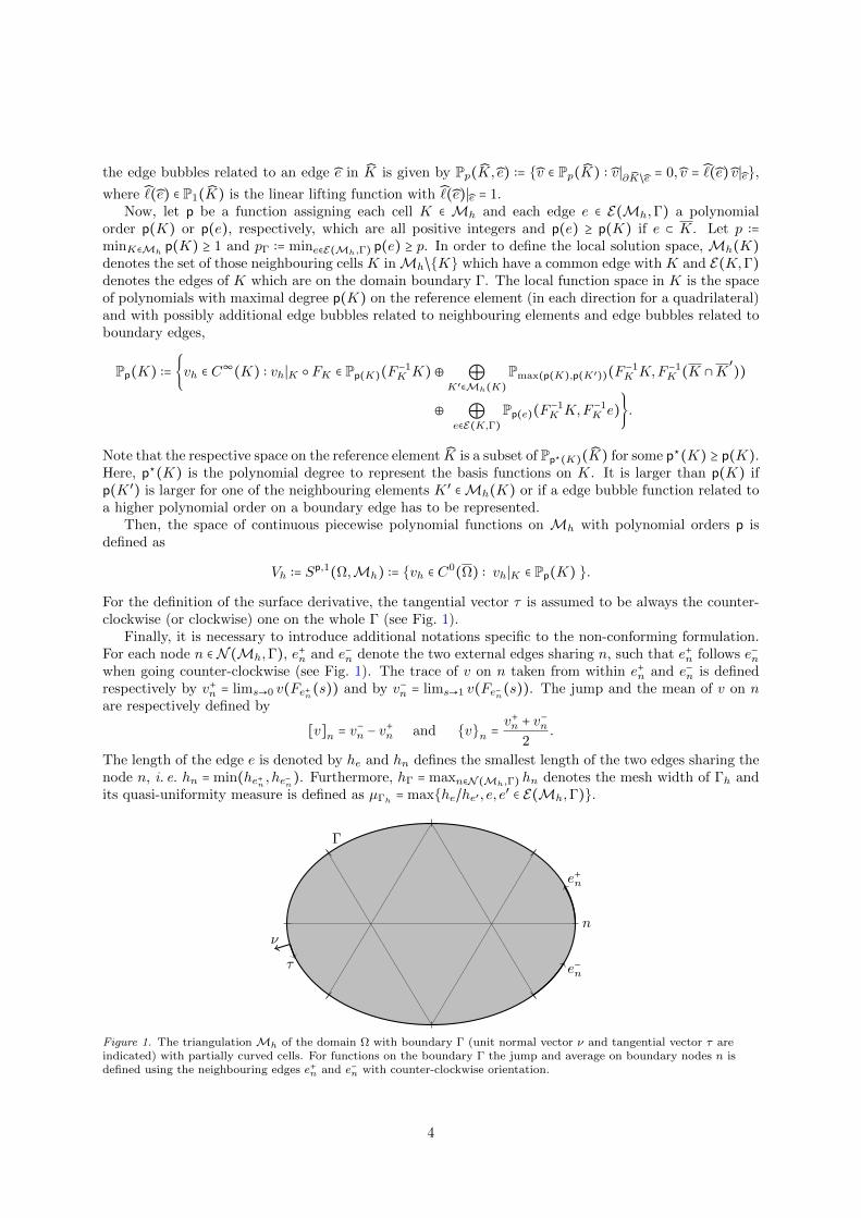
The presented non-conforming finite element method is based on a mesh Mh of the computationaldomain Ω (see Fig. 1) consisting of possibly curved triangles Th and curved quadrilaterals Qh, whichare disjoint and which fill the computational domain, i. e., Ω = ⋃K∈Mh

K. Each cell K in Th or Qh can

be represented through a smooth mapping FK from a single reference triangle K or a single referencequadrilateral K, respectively. The set of edges ofMh on Γ is denoted by E(Mh,Γ), N (Mh,Γ) is the setof nodes ofMh on Γ, and N (e) is the set composed of the two nodes of the external edge e. Furthermore,the union of all outer boundary edges and the union of all cells is defined as

Γh ∶= ⋃e∈E(Mh,Γ)

e = Γ/ ⋃n∈N (Mh,Γ)

n, Ωh ∶= ⋃K∈Mh

K = Ω/ ⋃e∈E(Mh)

e.

The edges E(Mh,Γ) of Mh are possibly curved, where for the analysis they are assumed to resolve Γexactly, i. e.,

Γ = ⋃e∈E(Mh,Γ)

e.

Furthermore, each edge is assumed to have counter-clockwise orientation and can be represented by asmooth mapping Fe from the reference interval (0,1). The mesh width h is the largest outer diameter ofthe cells

h ∶= maxK∈Mh

diam(K).

The discretization space will be defined in the following. First, K denotes a reference quadrilateralor triangle, respectively, and e denotes either one edge of K or the reference interval. Furthermore,Pp(K) denotes the space of polynomials of maximal total degree p for the reference triangle K and of

maximal degree p in each coordinate direction for the reference quadrilateral K. The space Pp(K) canbe decomposed into interior bubbles, edges bubbles to one of the edges and the nodal functions. Thespace of interior bubbles for the reference triangle is Pp(K,0) ∶= v ∈ Pp(K) ∶ v∣∂K = 0 and the one of

3

the edge bubbles related to an edge e in K is given by Pp(K, e) ∶= v ∈ Pp(K) ∶ v∣∂K/e = 0, v = (e) v∣e,

where (e) ∈ P1(K) is the linear lifting function with (e)∣e = 1.Now, let p be a function assigning each cell K ∈ Mh and each edge e ∈ E(Mh,Γ) a polynomial

order p(K) or p(e), respectively, which are all positive integers and p(e) ≥ p(K) if e ⊂ K. Let p ∶=minK∈Mh

p(K) ≥ 1 and pΓ ∶= mine∈E(Mh,Γ) p(e) ≥ p. In order to define the local solution space, Mh(K)

denotes the set of those neighbouring cells K inMh/K which have a common edge with K and E(K,Γ)

denotes the edges of K which are on the domain boundary Γ. The local function space in K is the spaceof polynomials with maximal degree p(K) on the reference element (in each direction for a quadrilateral)and with possibly additional edge bubbles related to neighbouring elements and edge bubbles related toboundary edges,

Pp(K) ∶= vh ∈ C∞(K) ∶ vh∣K FK ∈ Pp(K)(F

−1K K)⊕ ⊕

K′∈Mh(K)

Pmax(p(K),p(K′))(F−1K K,F −1

K (K ∩K′))

⊕ ⊕e∈E(K,Γ)

Pp(e)(F−1K K,F −1

K e).

Note that the respective space on the reference element K is a subset of Pp⋆(K)(K) for some p⋆(K) ≥ p(K).Here, p⋆(K) is the polynomial degree to represent the basis functions on K. It is larger than p(K) ifp(K ′) is larger for one of the neighbouring elements K ′ ∈Mh(K) or if a edge bubble function related toa higher polynomial order on a boundary edge has to be represented.

Then, the space of continuous piecewise polynomial functions on Mh with polynomial orders p isdefined as

Vh ∶= Sp,1

(Ω,Mh) ∶= vh ∈ C0(Ω) ∶ vh∣K ∈ Pp(K) .

For the definition of the surface derivative, the tangential vector τ is assumed to be always the counter-clockwise (or clockwise) one on the whole Γ (see Fig. 1).

Finally, it is necessary to introduce additional notations specific to the non-conforming formulation.For each node n ∈ N (Mh,Γ), e+n and e−n denote the two external edges sharing n, such that e+n follows e−nwhen going counter-clockwise (see Fig. 1). The trace of v on n taken from within e+n and e−n is definedrespectively by v+n = lims→0 v(Fe+n(s)) and by v−n = lims→1 v(Fe−n(s)). The jump and the mean of v on nare respectively defined by

[v]n = v−n − v

+n and vn =

v+n + v−n

2.

The length of the edge e is denoted by he and hn defines the smallest length of the two edges sharing thenode n, i. e. hn = min(he+n , he−n). Furthermore, hΓ = maxn∈N (Mh,Γ) hn denotes the mesh width of Γh andits quasi-uniformity measure is defined as µΓh

= maxhe/he′ , e, e′ ∈ E(Mh,Γ).

n

Γ

e+n

e−n

ν

τ

Figure 1. The triangulation Mh of the domain Ω with boundary Γ (unit normal vector ν and tangential vector τ areindicated) with partially curved cells. For functions on the boundary Γ the jump and average on boundary nodes n isdefined using the neighbouring edges e+n and e−n with counter-clockwise orientation.

4

3.2. Derivation of the interior penalty Galerkin variational formulation

First, the term ∂jΓαj∂jΓu for a function u ∈ C∞ is multiplied by vh ∈ Vh, which is in C∞(e) in each

edge on Γ. Then, j times integration by part is successively applied in each edge e to obtain

(−1)j ∫Γ∂jΓαj∂

jΓuvh dσ(x) = (−1)j ∑

e∈E(Mh,Γ)∫e∂jΓαj∂

jΓuvh dσ(x)

= ∑e∈E(Mh,Γ)

∫eαj∂

jΓu∂

jΓvh dσ(x) +

j−1

∑i=0

(−1)i+j ∑n∈N (Mh,Γ)

[∂j−i−1Γ αj∂

jΓu∂

iΓvh]n

= ∫Γαj∂

jΓu∂

jΓvh dσ(x) +

j−1

∑i=1

(−1)i+j ∑n∈N (Mh,Γ)

∂j−i−1Γ αj∂

jΓun[∂

iΓvh]n. (4)

Here, the equivalence [ab]n = [a]n bn + an [b]n is exploited, the fact that with uj , αj ∈ C∞ all jumps

[∂j−i−1Γ αj∂

jΓu]n, i < j are zero and that with vh ∈ C

0(Γ) all jumps [v]n are zero.If one is interested in symmetric bilinear forms to obtain the symmetric interior penalty Galerkin

formulation (SIPG) [49], it is necessary to add the terms s [∂iΓu]n∂j−i−1Γ αj∂

jΓvhn with s = 1 leading to

(−1)j ∫Γ∂jΓαj∂

jΓuvh dσ(x) = ∫

Γαj∂

jΓu∂

jΓvh dσ(x) (5)

+

j−1

∑i=1

(−1)i+j ∑n∈N (Mh,Γ)

(∂j−i−1Γ αj∂Γun [∂iΓvh]n + s [∂

iΓu]n ∂j−i−1

Γ αj∂Γvhn) .

There is no loss of consistency as with the assumption of u ∈ C∞(Γ) the terms [∂iΓu]n are in fact zero.Note that, alternatively, s = −1 for the non-symmetric (NIPG) [34] or s = 0 for the incomplete interiorpenalty Galerkin formulation (IIPG) [46] can be chosen.

Finally, to ensure the coercivity of the bilinear forms (with a mesh-independent constant), it remainsto add for j > 0 the terms

βj

h2(J−j)+1n

[∂j−1Γ u]

n[∂j−1

Γ vh]n ,

which also do not harm the consistency since [∂j−1Γ u]n = 0, j = 1, . . . , J − 1.

Remark 3.2. The assumption u ∈ C∞(Γ) in the derivation can be lowered. In fact u ∈ HJ(Γ), α0u ∈

L2(Γ), αj∂jΓu ∈ C

j−1(Γ)∩L2(Γ), j = 1, . . . , J is enough to ensure consistency. This requires αj ∈ L∞(Γ),

j = 0, . . . , J and with ∂jΓu ∈ Cj−1(Γ) for 2j ≤ J that αj ∈ C

j−1(Γ), j = 1, . . . , ⌊J2⌋. With these assumptions

it is indeed enough to require Γ to be Lipschitz and CJ,1 in a finite partition of the boundary. However,if u is solution of the above system it is unlikely to fulfill the regularity assumptions in this case [28].

Now, the interior penalty Galerkin formulation can be stated: Seek uJ,h ∈ Vh such that

aJ,h(uJ,h, vh) = ⟨fJ , vh⟩ , ∀vh ∈ Vh, (6)

where

aJ,h(uh, vh) ∶= ∫Ω(∇uh ⋅ ∇v − κ

2uhvh) dx +J

∑j=0

(cj(uh, vh;αj) + bj,h;J(uh, vh;αj))

cj(uh, vh;αj) ∶= ∫Γh

αj∂jΓuh ∂

jΓvh dσ(x) ,

b0,h;J = b1,h;J = 0 and for j > 1

bj,h;J(uh, vh;αj) ∶=j−1

∑i=1

(−1)i+j ∑n∈N (Mh,Γ)

(∂j−i−1Γ αj∂

jΓuhn[∂

iΓvh]n + s [∂

iΓuh]n∂

j−i−1Γ αj∂

jΓvhn)

+ ∑n∈N (Mh,Γ)

βj

h2(J−j)+1n

[∂j−1Γ uh]n[∂

j−1Γ vh]n ,

where s corresponds to the symmetric, non-symmetric or incomplete interior penalty method.

5

3.3. Well-posedness and estimation of the discretization error

If the finite element space is rich enough, the interior penalty formulation is well-posed and thediscretization error can be bounded as stated in the following two theorems. For this the so called brokennorm

∥v∥2VJ,h

∶= ∥v∥2H1(Ω) + ∥v∥2

HJ(Γh)(7)

is needed, as functions in Vh do not possess weak derivatives of order j = 2, . . . , J in the whole Γ, butonly in the open set Γh. Note, that for functions in VJ the ∥ ⋅ ∥VJ

-norm and the ∥ ⋅ ∥VJ,h-norm coincide.

The proofs of the following two theorems will be postponed to Sect. 5.

Theorem 3.3. Let infx∈Γ Re(αJ) > 0 or infx∈Γ ∣Im(αJ)∣ > 0 and let zero be the only solution of (3) withfJ = 0. Then, there exists constants hunique, punique > 0 such that for all h < hunique and p ≥ punique thediscrete interior penalty Galerkin variational formulation (6) for s ∈ [−1,1] and βj, j = 2, . . . , J largeenough admits a unique solution uJ,h ∈ Vh and there exists a constant CJ,h > 0 such that

∥uJ,h∥VJ,h≤ CJ,h∥fJ∥V ′

J. (8)

Theorem 3.4. Let J > 0, let the assumption of Theorem 3.3 be satisfied, let h < hunique, p ≥ punique,pΓ ≥ J and let the boundary mesh Γh be quasi-uniform, i. e., µΓh

< µΓ for some constant µΓ. Then, thereexists a constant CJ > 0 independent of Vh such that for the solution uJ,h ∈ Vh of (6) it holds

∥uJ,h − uJ∥VJ,h≤ CJ ( inf

vh∈Vh

∥vh − uJ∥H1(Ω) + hpΓ−J+1Γ ∥fJ∥V ′

J) . (9)

The first term in the right hand side of (9) is the H1-best-approximation error in the computationaldomain. It can be systematically decreased towards zero by mesh refinement or by increasing the polyno-mial degrees, possibly adaptively, especially in case of material corners (see e. g. [42] for p- and hp-finiteelement methods). The second term is due to the discretization of the surface differential operators inthe symmetric local absorbing boundary conditions. In order to achieve a convergent discretization, theminimum pΓ of the polynomial degrees on Γh has to be chosen to be at least J . For simple refinementof uniform meshes Mh (h-refinement) and polynomial degrees of at least p in the cells of Mh, the poly-nomial degrees on the edges of E(Mh,Γ) has to be chosen to be at least pΓ ≥ p + J − 1 such that theerror due to the discretization of the absorbing boundary condition does not dominate asymptotically forh→ 0.

3.4. Analysis of the computational costs

The proposed methodology requires J − 1 additional degrees of freedom per edge in E(Mh,Γ) whencomparing absorbing boundary conditions of order J to Neumann or Robin boundary conditions, whileclassical methodology requires the introduction of J−1 auxiliary unknowns and thus of p(J−1) additionaldegrees of freedom per edge in E(Mh,Γ). Note that, when considering odd order ABCs, the methodologyproposed by Hagstrom et.al. [23, 24] reduces this cost to (J − 1)/2 auxiliary unknowns and p(J − 1)/2degrees of freedom. Hence, the strategy developed in this paper is less costly and the higher the polynomialthe larger the computational costs are reduced.

3.5. Interior penalty formulation for terms with odd tangential derivatives

The proposed interior penalty formulation can be extended to the local boundary condition involvingterms with odd tangential derivatives of order 2J − 1 and less. To illustrate this point, it is sufficientto derive the additional term in the variational formulation on the example of the term ∂2

Γ(γ∂Γu) forγ ∈ C∞(Γ). In analogy to terms with even derivatives, an integration by parts on Γh and the use of thefact that [u]n = 0 on all n ∈ N (Mh,Γ) leads to

∫Γh

∂2Γ(γ∂Γu)v dσ(x) = −∫

Γh

∂Γ(γ∂Γu)∂Γv dσ(x).

6

Then, dividing the expression into two parts, applying integration by parts on one part, and using that[∂Γu]n = 0 on all n ∈ N (Mh,Γ), it reads

∫Γh

∂2Γ(γ∂Γu)v dσ(x) =

1

2∫

Γh

−∂Γ(γ∂Γu)∂Γv + γ∂Γu∂2Γv dσ(x) +

1

2∑

n∈N (Mh,Γ)

γn ∂Γun [∂Γv]n ,

where γn are the function values of γ on n ∈ N (Mh,Γ). Now, adding the terms sγn [∂Γu]n ∂Γvn relatedto the different variants of interior penalty formulations and using the identity γ∂Γu∂

2Γv = ∂Γu∂Γ(γ∂Γv)−

∂Γγ∂Γu∂Γv it follows that

∫Γh

∂2Γ(γ∂Γu)v dσ(x) =

1

2∫

Γh

∂Γu∂Γ(γ∂Γv) − ∂Γ(γ∂Γu)∂Γv dσ(x) −1

2∫

Γh

(∂Γγ)∂Γu∂Γv dσ(x)

+1

2∑

n∈N (Mh,Γ)

γn (∂Γun [∂Γv]n + s [∂Γu]n ∂Γvn) .

Obviously, the formulation with those additional terms related to odd derivatives loses symmetry evenfor s = 1. As only the highest derivatives in the formulation are crucial for coercivity no need to add anyfurther penalty term to ensure coercivity , whatever s is chosen.

4. Interior penalty finite element formulation in 3D

4.1. Local absorbing boundary conditions in 3D

In three dimensions, the gradient of a function u can be decomposed into a contribution normal tothe smooth surface Γ, that is ν∂νu = ν(∇u ⋅ ν), and a tangential gradient ∇Γu ∶= ∇u − ν∂νu. Similarly,the Laplacian ∆u can be decomposed into the second normal derivative ∂2

νu = ν⊺H(u)ν, where H is the

Hessian matrix with all partial second derivatives, and the Laplace-Beltrami operator ∆Γu ∶= ∆u − ∂2νu.

Note, that the latter is also given in terms of the surfacic divergence divΓ by ∆Γ ∶= divΓ∇Γ (see [31,Sect. 2.5.6] for their definition on smooth surfaces).

For example, the ABCs by Bayliss, Gunzburger and Turkel [6] (BGT) set on a spherical boundary Γof radius R are written in terms of the Laplace-Beltrami operator. For given wave number k, the BGTconditions of order 2 amount to

∂νu =1

2(−ik +

2

R)

−1

(∆Γ +2

R2+

4ik

R+ 2k2

)u =∶ B2u, (10)

where they serve as non-reflecting boundary conditions for the time-harmonic Helmholtz equation in 3D.If the shape of the boundary is arbitrary, but smooth, similar conditions were derived in [2]. Theseconditions include a term of the form divΓ(I −

ikR)∇Γ, where I is the identity and R the curvature

tensor. Non-reflecting boundary conditions for ellipsoidal boundaries were proposed in [5], and generalizedimpedance boundary conditions for highly conducting bodies of order 3 can be found in [22] in the formof Wentzell’s conditions.

All these conditions can be discretized directly with C0-continuous finite elements with an additionalbilinear form

∫Γαuv + (β∇Γu) ⋅ ∇ΓvdS(x),

only, where some scalar function α and some possibly tensorial function β appears.Patlashenko and Givoli [20, 32] introduce symmetric local absorbing boundary conditions of any

order J in three dimensions

∂νu =J

∑j=0

αj (−1)j∆jΓu, (11)

where αj are scalar constants. In this case, (11) can be seen as a generalization of (1) with constantparameters αj in three dimensions. The parameters αj were computed by Harari in [25] in the specificcase where the artificial boundary is a sphere.

7

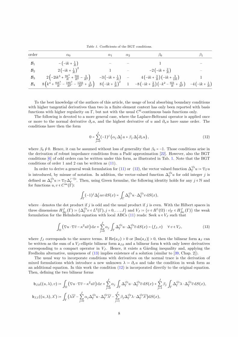
Table 1. Coefficients of the BGT conditions.

order α0 α1 α2 β0 β1

B1 − (−ik + 1R) – – 1 –

B2 2 (−ik + 1R)

21 – −2 (−ik + 2

R) –

B3 2 (−2ik3 + 9k2

R+ 9ikR2 −

3R3 ) −3 (−ik + 1

R) – 4 (−ik + 3

R) (−ik + 3

2R) 1

B4 8 (k4 + 8ik3

R− 18k2

R2 − 12ikR3 + 3

R4 ) 8 (−ik + 3R)

21 −8 (−ik + 2

R) (−k2 − 6ik

R+ 6R2 ) −4 (−ik + 1

R)

To the best knowledge of the authors of this article, the usage of local absorbing boundary conditionswith higher tangential derivatives than two in a finite element context has only been reported with basisfunctions with higher regularity on Γ, but not with the usual C0-continuous basis functions only.

The following is devoted to a more general case, where the Laplace-Beltrami operator is applied onceor more to the normal derivative ∂νu, and the highest derivative of u and ∂nu have same order. Theconditions have then the form

0 =J

∑j=0

(−1)j (αj ∆jΓu + βj ∆j

Γ∂νu) , (12)

where β0 /= 0. Hence, it can be assumed without loss of generality that β0 = −1. Those conditions arise inthe derivation of robust impedance conditions from a Pade approximation [22]. However, also the BGTconditions [6] of odd orders can be written under this form, as illustrated in Tab. 1. Note that the BGTconditions of order 1 and 2 can be written as (11).

In order to derive a general weak formulation for (11) or (12), the vector valued function ∆1/2

Γ u ∶= ∇Γu

is introduced, by misuse of notation. In addition, the vector-valued function ∆j/2

Γ u for odd integer j is

defined as ∆j/2

Γ u ∶= ∇Γ∆j−1/2

Γ . Then, using Green formulae, the following identity holds for any j ∈ N andfor functions u, v ∈ C∞(Γ):

∫Γ(−1)j∆j

Γuv dS(x) = ∫Γ

∆j/2

Γ u ⋅∆j/2

Γ v dS(x),

where ⋅ denotes the dot product if j is odd and the usual product if j is even. With the Hilbert spaces in

three dimensions HJ∆Γ

(Γ) ∶= ∆j/2

Γ v ∈ L2(Γ), j = 0, . . . , J and VJ ∶= v ∈ H1(Ω) ∶ v∣Γ ∈ HJ∆Γ

(Γ) the weakformulation for the Helmholtz equation with local ABCs (11) reads: Seek u ∈ VJ such that

∫Ω(∇u ⋅ ∇v − κ2uv)dx +

J

∑j=0

αj ∫Γ

∆j/2

Γ u ⋅∆j/2

Γ v dS(x) = ⟨fJ , v⟩ ∀ v ∈ VJ , (13)

where fJ corresponds to the source terms. If Re(aJ) > 0 or ∣Im(aJ)∣ > 0, then the bilinear form aJ canbe written as the sum of a VJ -elliptic bilinear form aJ,0 and a bilinear form k with only lower derivativescorresponding to a compact operator in VJ . Hence, it exists a Garding inequality and, applying theFredholm alternative, uniqueness of (13) implies existence of a solution (similar to [39, Chap. 2]).

The usual way to incorporate conditions with derivatives on the normal trace is the derivation ofmixed formulations which introduce a new unknown λ ∶= ∂νu and take the condition in weak form asan additional equation. In this work the condition (12) is incorporated directly to the original equation.Then, defining the two bilinear forms

bJ,0((u,λ), v) ∶= ∫Ω(∇u ⋅ ∇v − κ2uv)dx +

J

∑j=0

αj ∫Γ

∆j/2

Γ u ⋅∆j/2

Γ v dS(x) +J

∑j=1

βj ∫Γ

∆j/2

Γ λ ⋅∆j/2

Γ v dS(x),

bJ,1((u,λ), λ′) ∶= ∫

Γ(λλ′ −

J

∑j=0

αj∆j/2

Γ u ⋅∆j/2

Γ λ′ −J

∑j=1

βj∆j/2

Γ λ ⋅∆j/2

Γ λ′)dS(x),

8

the mixed variational formulation for the Helmholtz equation with (12) on Γ reads as: Seek (u,λ) ∈

VJ ×HJ∆Γ

(Γ) such that

bJ((u,λ), (v, λ′)) ∶= bJ,0((u,λ), v) + bJ,1((u,λ), λ

′) = ⟨fJ , v⟩ ∀ (v, λ′) ∈ VJ ×H

J∆Γ

(Γ). (14)

Using test functions (v,0) and (0, λ′) it easy to see that the two equations in the volume and on theartificial boundary are separately enforced. Equivalently to the two separate equations, the variationalformulation bJ,0((u,λ), v) + γJbJ,1((u,λ), λ′) = ⟨fJ , v⟩ can be considered, where the conjugate complexof the second equation is taken and γJ /= 0 is an arbitrary complex factor. Then, with the choice v = u,λ′ = λ and γJ =

βJ

αJ, the mixed terms of highest order cancel out and

bJ,0((u,λ), u) +βJαJ

bJ,1((u,λ), λ) = ∣u∣2H1(Ω) + αJ ∣u∣2HJ

∆Γ(Γ) −

∣βJ ∣2

αJ∣λ∣2HJ

∆Γ(Γ)

+ ⟨κu,u⟩L2(Ω)

+J−1

∑j=0

αj ∣u∣2Hj

∆Γ(Γ)

+βJαJ

(∥λ∥L2(Γ) −J−1

∑j=1

βj ∣λ∣2Hj

∆Γ(Γ)

)

+J−1

∑j=1

(βj −βJαJ

αj)⟨∆j/2

Γ λ,∆j/2

Γ u⟩L2(Γ)

−βJαJ

α0⟨λ,u⟩ .

Here, the seminorms ∣ ⋅ ∣Hj∆Γ(Γ) ∶= ∥∆

j/2

Γ ⋅ ∥L2(Γ), j = 0, . . . , J were used. If ∣Im(aJ)∣ > 0 and βJ /= 0 then

there holds a Garding inequality, i. e., there exists a constant θ ∈ (−π,π) and

Re(eiθ(bJ,0((u,λ), u) +βJαJ

bJ,1((u,λ), λ))) ≥ γ (∥u∥2VJ

+ ∥λ∥2HJ

∆Γ(Γ)) − δ (∥u∥

2WJ−1

+ ∥λ∥2HJ−1

∆Γ(Γ)) ,

for some constants γ > 0 and δ ∈ R, where WJ−1 ∶= L2(Ω) ∩HJ−1

∆Γ(Γ). Since VJ ⊂⊂WJ−1 and HJ

∆Γ(Γ) ⊂⊂

HJ−1∆Γ

(Γ) the Fredholm alternative applies as well and there exists a unique solution of (14), except for aset of spurious eigenmodes.

4.2. Definition of the C0-continuous finite element spacesSimilarly to the two-dimensional case, the non-conforming finite element method is based on a mesh

Mh of the computational domain Ω consisting of possibly curved tetrahedra, hexahedra, prism or pyra-mids, which are disjoint and which fill the computational domain, i. e., Ω = ⋃K∈Mh

K. The set of faces(triangles or quadrilaterals) of Mh on Γ is denoted by F(Mh,Γ), E(Mh,Γ) is the set of edges of Mh

on Γ and E(e) is the set composed of all the edges of the external boundary Γ. Furthermore, the unionof all outer boundary faces and the union of all cells is defined as

Γh ∶= ⋃f∈F(Mh,Γ)

f = Γ/ ⋃e∈E(Mh,Γ)

e, Ωh ∶= ⋃K∈Mh

K = Ω/ ⋃f∈F(Mh)

f.

It is assumed that each face can be represented by a smooth mapping Ff from the reference triangle

or quadrilateral F . As in 2D, the mesh width h is the largest outer diameter of the cells and Vh ∶=

Sp,1(Ω,Mh) denotes the space of piecewise continuous polynomial functions on Mh with polynomialorders p.

Finally, additional notations specific to the non-conforming formulation are introduced. For each edgee ∈ E(Mh,Γ), the two external faces sharing e are arbitrarily denoted by f+e and f−e and the trace of von e taken from within f+e and f−e is defined respectively by v+e and by v−e . Furthermore, on an edge e ofa face f ∈ F(Mh,Γ), the outward unit normal vector of f on e (orthogonal to ν) is denoted by τe. Thejump and the mean of a scalar function v on e are respectively defined by

[v]e = v−e − v

+e and ve =

v+e + v−e

2,

while the jump and the mean of a vectorial function v on e are respectively defined by

[v]e = v−e ⋅ τ

−e + v

+e ⋅ τ

+e and ve =

v−e ⋅ τ−e − v

+e ⋅ τ

+e

2.

The diameter of the face f is denoted by hf and he defines the smallest diameter of the two faces sharingthe edge e, i. e., he = min (hf+e , hf−e ).

9

4.3. Definition of the interior penalty Galerkin variational formulation

The construction of the interior penalty Galerkin formulation is similar to the 2D case. First,

∆j/2

Γ αj∆j/2

Γ u for a function u ∈ C∞ is multiplied by vh ∈ Vh, which is in C∞(f) in each face f on Γ,and j-times integration by part are successively applied in each face f . Second, the equivalence [ab]e =

[a]e be+ae [b]e is exploited, the fact that with uj , αj ∈ C∞ all jumps [∆

(j−i−1)/2Γ αj∆

j/2

Γ u]e, i < j are zero

and that with vh ∈ C0(Γ) all jumps [v]

eare zero. Third, the terms s ∫e[∆

i/2

Γ u]e∆(j−i−1)/2Γ αj∆

j/2

Γ vhe dσ(x)are added, with s = 1 for SIPG, s = −1 for NIPG and s = 0 for IPDG. There is no loss of consistency

since the terms [∆i/2

Γ u]e are in fact zero due to the assumption that u ∈ C∞(Γ). Finally, to ensure thecoercivity of the bilinear forms (with a mesh-independent constant), the terms

βj

h2(J−j)+1e

∫e[∆

j−1/2

Γ u]e[∆j−1/2

Γ vh]e dσ(x)

are added for j > 0, which does not harm the consistency since [∆j−1/2

Γ u]e = 0, j = 1, . . . , J − 1.The interior penalty Galerkin formulation reads then: Seek uJ,h ∈ Vh such that

aJ,h(uJ,h, vh) = ⟨fJ , vh⟩ , ∀vh ∈ Vh, (15)

where

aJ,h(uh, vh) ∶= ∫Ω(∇u ⋅ ∇v − κ2uv)dx +

J

∑j=0

(∫Γh

αj∆j/2

Γ uh ⋅∆j/2

Γ vh dS(x) + bj,h(uh, vh))

and b0,h = b1,h = 0 and for j > 1

bj,h(uh, vh) ∶=j−1

∑i=1

(−1)i+j ∑e∈E(Mh,Γ)

∫e(∆

(j−i−1)/2Γ αj∆

j/2

Γ uhe[∆i/2

Γ vh]e + s[∆i/2

Γ uh]e∆(j−i−1)/2Γ αj∆

j/2

Γ vhe) dσ(x)

+ ∑e∈E(Mh,Γ)

βj

h2(J−j)+1e

∫e[∆

j−1/2

Γ uh]e[∆j−1/2

Γ vh]e dσ(x).

5. Analysis of the interior penalty formulation in 2D

5.1. Associated variational formulation for infinite-dimensional spaces

The objective of this subsection is, in analogy to [21], the definition of an interior-penalty Galerkinvariational formulation which is identical to the discrete one for the discrete space Vh and which can bedefined for infinite-dimensional function spaces as well. As the discrete space Vh is not contained in thecontinuous function spaces VJ for J ≥ 2, it is necessary to use larger spaces VJ,h, which include both Vhand VJ . These infinite-dimensional spaces are defined by

VJ,h ∶= v ∈H1(Ω) ∶ v∣Γ ∈H1

(Γ) ∩HJ(Γh) ⊃ VJ . (16)

Note, that the trace of functions v ∈ VJ,h is continuous on Γ and their tangential derivatives of order 1 toJ − 1 are bounded, but may be discontinuous over the nodes N (Mh,Γ). In addition to the broken normdefined in (7) the norm

∥v∥2

VJ,h,IP∶= ∥v∥

2

H1(Ω)+ ∥v∥

2

HJ(Γh)+

J

∑j=2

∑n∈N (Mh,Γ)

1

h2(J−j)+1n

∣[∂j−1Γ v]

n∣2

(17)

with penalty terms on the boundary nodes n will be used. These norms are equivalent, however, withconstants depending on the edge lengths hn.

The discrete formulation (6) cannot directly be used with the function space VJ,h since the terms

∂j−i−1Γ αj∂

jΓun are not well-defined for 2j − i > J if u ∈ VJ,h. In the discrete variational formulation,

10

those terms occur only in product with the finitely many piecewise polynomials in Vh. An extensionof these products to functions u ∈ VJ,h can be defined using the lifting operators Lj,i ∶ H

1(Γh) → Vh,i, j ∈ N by

∫Γh

Lj,i(v)αj∂jΓwh dσ(x) = ∑

n∈N (Mh,Γ)

[v]n∂j−i−1Γ αj∂

jΓwhn ∀wh ∈ Vh. (18)

Then, any occurrence of ∑n∈N (Mh,Γ) ∂j−i−1Γ αj∂

jΓuhn[∂

iΓvh]n or of its symmetric counterpart in the

discrete formulation (6) is replaced by ∫Γhαj∂

jΓuLj,i(∂

iΓv)dσ(x) or by its symmetric counterpart, respec-

tively.Now, the interior penalty Galerkin variational formulation for the infinite-dimensional spaces VJ,h

reads as: Seek uJ ∈ VJ,h such that

aJ,h(uJ , v) = ⟨fJ,h, v⟩ , ∀v ∈ VJ,h, (19)

where

aJ,h(u, v) ∶= ∫Ω(∇uJ ⋅ ∇v − κ

2uJv) dx +J

∑j=0

(cj(uh, vh;αj) + bj,h;J(u, v;αj))

and for b0,h;J = b1,h;J = 0 and for j > 1

bj,h;J(u, v;αj) ∶=j−1

∑i=1

(−1)i+j ∫ΓαjLj,i(∂

iΓu)∂

jΓv + sαjLj,i(∂

iΓv)∂

jΓudσ(x)

+ ∑n∈N (Mh,Γ)

βj

h2(J−j)+1n

[∂j−1Γ u]

n[∂j−1

Γ v]n.

Note that, due to the definition of the lifting operators, bj,h;J = bj,h;J on Vh×Vh and bj,h;J = 0 on Vj ×Vj ,as all jump terms and so all lifting operators vanish and the weak derivatives exists on the whole Γ, notonly on Γh. Hence, aJ,h = aJ,h on Vh × Vh and aJ,h = aJ on VJ × VJ .

5.2. Analysis of the associated variational formulation

The following lemma states the equivalence of (3) and (19).

Lemma 5.1. Let ⟨fJ , v⟩ = ∫Ω fv dx + ∫Γ gv dσ(x) with f ∈ L2(Ω) and g ∈ L2(Γ). Then, the formula-tions (3) and (19) possess the same solutions, i. e., if uJ ∈ VJ is solution of (3), then it solves (19), andif uJ ∈ VJ,h is solution of (19), then it solves (3).

Proof. If J = 0,1, then the formulations (3) and (19) are identical, and the proof continues with J ≥ 2.The proof is in two steps. First, it is proven that the solution uJ ∈ VJ of (3) solves (19), and then, thatthe solution uJ ∈ VJ,h of (19) solves (3).

(i) Let uJ ∈ VJ be solution of (3). Choosing test functions v ∈ C∞c (Ω) ⊂H1

0(Ω) vanishing on ∂Ω in (3)and using the definition of weak derivatives, it follows that that uJ solves

−∆uJ − κ2uJ = f in Ω. (20a)

If ∂Ω/Γ is non empty, test functions v can be chosen in v ∈ H1(Ω) with v ≡ 0 on Γ. Then, usingintegration by parts in Ω and the fact that uJ solves (20a) one can show that uJ solves

∂νuJ = 0 on ∂Ω/Γ. (20b)

Now, taking test functions v in the whole space VJ , using integration by parts in Ω and on Γ, andusing the fact that uJ solves (20a) and (20b) it holds in the same way

∂νuJ +J

∑j=0

(−1)j∂jΓ(αj∂jΓuJ) = g on Γ. (20c)

11

Following the same steps as for the construction of the bilinear form aJ,h (but using the liftingoperators instead of the jump terms), it follows easily that uJ solves aJ,h(uJ , v) = ⟨fJ,h, v⟩ for allv ∈ VJ,h.

(ii) Let uJ ∈ VJ,h solution of (19). In the same way as in Part (i), it can be proven that uJ solves (20a)

and (20b). Now, let the test function v ∈ VJ ∩C∞c (Γh) such that bj(u, v) = bj,h(u, v) holds for any

u ∈ VJ . Then using integration by parts in Ω, and the fact that uJ solves (20a) and (20b), it followsthat uJ solves (20c) on Γh.

Comparing with the integration by parts formula in (4) this proves that for all v ∈ VJ ∩C∞(Γh)

J

∑j=2

∑n∈N (Mh,Γ)

(

j−1

∑i=1

(−1)i+j ([∂j−i−1Γ αj∂

jΓuJ]n∂

iΓvn − s[∂

iΓuJ]n∂

j−i−1Γ αj∂

jΓvn)

+βj

h2(J−j)+1n

[∂j−1Γ uJ]n[∂

j−1Γ v]

n) = 0.

Let now the test function v ∈ VJ ∩C∞(Γh) such that it holds ∂j−1

Γ vn= 0 for all j = 2, . . . , J and

all n ∈ N (Mh,Γ) and such that ∂j−i−1Γ αj∂

jΓvn = 0 for all j = 2, . . . , J and i = 1, . . . , j − 1 if s /= 0.

Then it holds that

J

∑j=2

∑n∈N (Mh,Γ)

βj

h2(J−j)+1n

[∂j−1Γ uJ]n[∂

j−1Γ v]

n= 0.

This is only possible if [∂j−1Γ uJ]n = 0 for j = 2, . . . , J and any n ∈ N (Mh,Γ).

Hence, this proves that uJ is in VJ and solves (20) and so (3).

This completes the proof.

The following lemmata are required to prove the well-posedness of the variational formulation (19).

Lemma 5.2. The lifting operators Lj,i ∶H1(Γh)→ Vh, i, j ∈ N defined by (18) are continuous, i. e., there

exists constants Cj,i > 0 such that

∥Lj,i(v)∥2L2(Γ) ≤ C

2j,i ∑n∈N (Mh,Γ)

∣[v]n∣2

h2(j−i)−1n

.

Proof. From the definition of the mean over n, it holds

∣∂j−i−1Γ αj∂

jΓwhn∣

2≤

∣(∂j−i−1Γ αj∂

jΓwh)

+n∣

2+ ∣(∂j−i−1

Γ αj∂jΓwh)

−n∣

2

2, (21)

with the notation (v)±n = v±n. Now, using inverse inequalities [42, 48] and the fact that hn ≤ he±n , it reads

∣(∂j−i−1Γ αj∂

jΓwh)

±n∣

2≤

C2j,i

2h2(j−i)−1n

∫e±n

∣αj∂jΓwh∣

2 dσ(x) (22)

with Cj,i ∶= Cj,i(pΓ) = O(p2(j−i)−1Γ ), and using (21) yields

∣∂j−i−1Γ αj∂

jΓwhn∣

2≤

C2j,i

2h2(j−i)−1n

∫e+n∪e−n

∣αj∂jΓwh∣

2 dσ(x)

and so

∑n∈N (Mh,Γ)

h2(j−i)−1n ∣∂j−i−1

Γ αj∂jΓwhn∣

2≤ C2

j,i∥αj∂jΓwh∥

2L2(Γ). (23)

12

Then, using the definition of the lifting operator Lj,i and the Cauchy-Schwarz-inequality, it follows that

∥Lj,i(v)∥2L2(Γ) = max

wh∈Vh

∣ ∑n∈N (Mh,Γ)

[v]n ∂j−i−1Γ αj∂

jΓwhn ∣

2

∥αj∂jΓwh∥

2L2(Γ)

≤ maxwh∈Vh

∑n∈N (Mh,Γ)

∣[v]n∣2

h2(j−i)−1n

∑n∈N (Mh,Γ)

h2(j−i)−1n ∣∂j−i−1

Γ αj∂jΓwhn∣

2

∥αj∂jΓwh∥

2L2(Γ)

.

Finally, inserting (23), and the statement of the lemma is proved.

Lemma 5.3. Let s ∈ [−1,1], J ≥ 1, αJ ∈ L∞(Γ) with infx∈Γ Re(αJ) > 0 or infx∈Γ ∣Im(αJ)∣ > 0. Then, for

βj large enough the bilinear form a0,J defined by

a0,J(u, v) ∶= ∫Ω(∇u ⋅ ∇v + uv) dx +

J−1

∑j=0

(cj,h(u, v; 1) + bj,h;J(u, v; 1)) + cJ,h(u, v; 1) + bJ,h;J(u, v;αJ),

(24)

is VJ,h-elliptic with an ellipticity constant independent of hn for all n ∈ N (Mh,Γ) when measured in the∥ ⋅ ∥VJ,h,IP

-norm.

The proof is a simple consequence of the following lemma, in which a more explicit statement howlarge the penalty terms βj need to be is given.

Lemma 5.4. Let the assumption on s and αJ in Lemma 5.3 be fulfilled. Then, there exist constantsC, γ and θ, such that the following inequality holds for βj >

√j C, j ≥ 2:

Re(eiθJ−1

∑j=0

(cj,h(v, v; 1) + bj,h;J(v, v; 1))) +Re(eiθ(cJ,h(v, v;αJ) + bJ,h;J(v, v;αJ)))

≥ γ⎛

⎝∥v∥2

HJ(Γ) +J

∑j=2

∑n∈N (Mh,Γ)

1

h2(J−j)+1n

∣[∂j−1Γ v]

n∣2⎞

⎠∀v ∈Hj

(Γh) .

Proof. With the assumption on αJ there exists θ ∈ (−π2, π

2) such that it holds

Re(eiθ∫

ΓαJ ∣v∣

2) ≥ γJ ∣v∣

2L2(Γ), (25)

with a positive constant γJ . In the remainder of the proof it is assumed that θ is such that (25) is fulfilled.The first step of the proof is to write

Re (eiθbj,h;J(v, v;αj)) =j−1

∑i=1

(−1)i+j Re(eiθ∫

ΓαjLj,i(∂

iΓv)∂

jΓv + sαjLj,i(∂

iΓv)∂

jΓv dσ(x))

+ cos(θ) ∑n∈N (Mh,Γ)

βj

h2(J−j)+1n

∣[∂j−1Γ v]

n∣2.

Using that 2ab ≤ εa2 + ε−1b2 for any positive ε, the fact that αj = 1 for j < J in the bilinear forms bj,h;J ,the assumption on αJ and Lemma 5.2, the estimate

2 ∣∫ΓαjLj,i(∂

iΓv)∂

jΓv dσ(x)∣ ≤ ε∥∂jΓv∥

2L2(Γ) + ε

−1∥αjLj,i(∂

iΓv)∥

2L2(Γ)

≤ ε∥∂jΓv∥2L2(Γ) + ε

−1∥αj∥

2L∞(Γ)C

2j,i ∑n∈N (Mh,Γ)

1

h2(j−i)−1n

∣ [∂iΓv]n ∣2 ,

13

follows. Obviously, the same bound holds, if v and v are interchanged. Consequently, it follows that

Re(eiθJ−1

∑j=0

(cj,h(v, v; 1) + bj,h;J(v, v; 1))) +Re(eiθ(cJ,h(v, v;αJ) + bJ,h;J(v, v;αJ)))

≥ cos(θ)∥v∥2

H1(Γ)+J−1

∑j=2

( cos(θ) − (j − 1) εj)∥∂jΓv∥

2

L2(Γ)+ (γJ − (J − 1) εJ)∥∂

JΓv∥

2

L2(Γ)

+J

∑j=2

∑n∈N (Mh,Γ)

⎛

⎝

cos(θ)βj

h2(J−j)+1n

−J

∑i=j

ε−1i ∥αi∥L∞(Γ)

C2i,j−1

h2(i−j)+1n

⎞

⎠∣[∂j−1

Γ v]n∣2.

Finally, choosing εj = cos(θ)/j for j = 2, . . . , J − 1 and εJ = γJ/J , and with the assumption on βj , thedesired inequality is obtained.

The following two theorems state the main results for the variational formulation (19).

Theorem 5.5. Let the assumption of Lemma 5.4 be satisfied, and let zero be the only solution of (19)with uinc ≡ 0. Then, there exists a unique solution uJ ∈ VJ,h of (19) and there exists a constant CJ > 0independent of hn for all n ∈ N (Mh,Γ) such that

∥uJ∥VJ,h,IP≤ CJ∥fJ,h∥V ′

J,h,IP.

Proof. The proof is along the lines of that of [39, Theorem 2.3]. By Lemma 5.3 the bilinear form a0,J is

VJ,h-elliptic and so the associated operators A0,J are isomorphisms in VJ,h. Let the Sobolev spaces

W0,h ∶= L2(Ω), WJ,h ∶= L

2(Ω) ∩HJ−1

(Γh), J > 0,

be defined, where the Rellich-Kondrachov compactness theorem [1, Chap. 6] implies that the embeddingVJ,h ⊂⊂WJ,h is compact. Now, the operators KJ associated to the bilinear forms

kJ(u, v) ∶= −∫Γ(κ2

+ 1)uv dx +J−1

∑j=0

(cj,h(u, v;αj − 1) + bj,h;J(u, v;αj − 1)) , J > 0,

are compact.Hence, the operators A0,J + KJ associated to the bilinear forms aJ = a0,J + kJ are Fredholm with

index 0 and by the Fredholm alternative [36, Sec. 2.1.4] the uniqueness of a solution of (3) implies itsexistence and its continuous dependence on the right hand side with constants independent of hn for alln ∈ N (Mh,Γ), and the proof is complete.

Theorem 5.6. Let the assumption of Lemma 5.5 be satisfied, and let c−1 ∈ L∞loc(R2) fixed with c(x) =c0 > 0 for ∣x∣ > RC and κ(x) = ω/c(x) with the frequency ω > R+. Then, (19) has a unique solution exceptfor a countable (possibly finite) set of frequencies ω, the spurious eigenfrequencies, which accumulatesonly at infinity. The set of these frequencies coincides with the one of (3).

Proof. Using Lemma 5.1, the proof of this statement is analog to the proof of [39, Lemma 2.6].

Remark 5.7. As the solution uJ ∈ VJ,h of (19) coincides with uJ ∈ VJ of (3) and as the eigenfrequenciescoincide, the guaranteed uniqueness in case of Feng’s absorbing boundary conditions for large enoughdomains by [39, Lemma 2.7] apply to uJ as well.

5.3. Analysis of the discrete discontinuous Galerkin variational formulation

The discrete discontinuous Galerkin variational formulation (6) is the Galerkin discretization of theassociated variational formulation (19), when using Vh as the finite-dimensional subspace of VJ,h.

14

Proof of Theorem 3.3. By the assumption that zero is the only solution of the continuous variationalformulation (3) with zero sources, there exist a function c(x) and a frequency ω such that κ(x) = ω/c(x)as in [39, Lemma 2.6] and such that ω is not a spurious eigenfrequency. For J = 0 and ∣Im α0∣ > 0 thestatement of the theorem was proved by Melenk and Sauter [30, Thm. 5.8].

The discrete system (6) is the Galerkin discretization of (19), which has by Theorem 5.6, with κ(x) =ω/c(x), the same eigenfrequencies as (3). Both systems are non-linear in ω and can be regarded in asimilar fix-point form, as in [39, Eq. (2.6)]. These systems are linear eigenvalue problems in ω2 for givenparameter ω ∈ C/0, where the fix-point system of (19) admits a countable set of frequencies ωm(ω) andthat of (6) a finite set ωm,h(ω). As ω is not a spurious eigenfrequency, ωm(ω) /= ω for any m ∈ N, and sothe distances of the curves ωm(ω) to the point ω = ω are positive. Let dm, m ∈ N denote these distances.

By the Babuska-Osborn theory [4] the discrete eigenfrequencies, ωm,h(ω) tend to ωm(ω) if the mesh-widths tend to zero for a minimal polynomial degree, which depends on J , or if the polynomial degreestend to infinity. As a consequence, the distance dm,h of the curve ωm,h(ω) to the point ω = ω tends todm, and for a fine enough mesh or large enough polynomial degrees ∣dm,h − dm∣ < 1

2dm, and so dm,h > 0.

This means that ω is not an eigenfrequency of the discrete variational problem (6). Hence, it admits aunique solution [36, Sec. 2.1.6] bounded by (8).

This completes the proof.

Proof of Theorem 3.4. First, to follow up directly the proof of Theorem 3.3 the observation that thebilinear form aJ,h of the interior penalty Galerkin formulation satisfies a Garding inequality implies itsasymptotic quasi-optimality in the VJ,h,IP-norm, see [9, 37] and [30, Sec. 3.2], i. e.,

∥uJ,h − uJ∥VJ,h,IP≤ C inf

vh∈Vh

∥vh − uJ∥VJ,h,IP, (26)

where C denotes throughout the proof a constant not depending on Vh.To estimate the jump terms in the definition of the VJ,h,IP-norm, see (17), let on any edge e ∈ E(Mh,Γ)

the pullback of vh and uJ to the reference interval [0,1] be denoted by (vh)e and (uJ)e. Then, using thetrace theorem twice on the reference interval it follows for any j = 2, . . . , J and any n ∈ N (Mh,Γ) that

1

h2(J−j)+1n

∣[∂j−1Γ (vh − uJ)]n∣

2≤

C

h2J−1n

(∣∂j−1s ((vh)e+n − (uJ)e+n)∣s=0∣

2+ ∣∂j−1

s ((vh)e−n − (uJ)e−n)∣s=1∣2)

≤C

h2J−1n

(∥(vh)e+n − (uJ)e+n)∥2Hj(0,1) + ∥(vh)e−n − (uJ)e−n)∥

2Hj(0,1))

≤ Cj

∑`=0

1

h2(J−`)n

(∣vh − uJ ∣2H`(e+n)

+ ∣vh − uJ ∣2H`(e−n)

) ,

where s denotes the local coordinate in [0,1].Hence, it follows for any vh ∈ Vh that

∥vh − uJ∥2VJ,h,IP

= ∥vh − uJ∥2H1(Ω) +

J

∑j=1

∣vh − uJ ∣2Hj(Γh)

+J

∑j=2

∑n∈N (Mh,Γ)

1

h2(J−j)+1n

∣[∂j−1Γ (vh − uJ)]n∣

2

≤ C (∥vh − uJ∥2H1(Ω) +

J

∑j=0

1

h2(J−j)Γ

∣vh − uJ ∣2Hj(Γh)

) . (27)

To obtain optimal bounds for the terms on Γh the function vh is replaced by the Raviart-Thomas inter-polation operator IΓ,huJ on the trace space TVh(Γ) of Vh on Γ, for which it holds [11, Chap. 3]

(hJ−jΓ )−1

∣IΓ,huJ − uJ ∣Hj(Γh) ≤ C hpΓ−J+1Γ ∥uJ∥HpΓ+1(Γ) ≤ C h

pΓ−J+1Γ ∥fJ∥V ′

J. (28)

Here, [39, Lemma 2.8] was used to obtain the last inequality.To estimate the first term in (27) the function vh is replaced by the H1(Ω)-projection QΩ,h ∶ VJ,h → Vh,

for which QΩ,h ⋅ ∣Γ = IΓ,h⋅. Then,

∫Ω∇(QΩ,huJ − uJ) ⋅ ∇wh + (QΩ,huJ − uJ)wh dx = 0 ∀wh ∈ Vh,0,

15

(a)

RD

R

ΓΩ

(b)

a

d

R

Γ = ∂ΩΩ

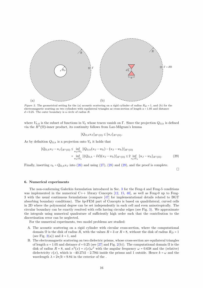
Figure 2. The geometrical setting for the (a) acoustic scattering on a rigid cylinder of radius RD = 1, and (b) for theelectromagnetic scatting on two cylinders with equilateral triangles as cross-section of length a = 1.05 and distanced = 0.25. The outer boundary is a circle of radius R.

where Vh,0 is the subset of functions in Vh whose traces vanish on Γ. Since the projection QΩ,h is definedvia the H1(Ω)-inner product, its continuity follows from Lax-Milgram’s lemma

∥QΩ,huJ∥H1(Ω) ≤ ∥uJ∥H1(Ω).

As by definition QΩ,h is a projection onto Vh it holds that

∥QΩ,huJ − uJ∥H1(Ω) ≤ infwh∈Vh

∥QΩ,h(uJ −wh) − (uJ −wh)∥H1(Ω)

= infwh∈Vh

∥(QΩ,h − Id)(uJ −wh)∥H1(Ω) ≤ 2 infvh∈Vh

∥uJ −wh∥H1(Ω). (29)

Finally, inserting vh = QΩ,huJ into (26) and using (27), (28) and (29), and the proof is complete.

6. Numerical experiments

The non-conforming Galerkin formulation introduced in Sec. 3 for the Feng-4 and Feng-5 conditionswas implemented in the numerical C++ library Concepts [12, 15, 40], as well as Feng-0 up to Feng-3 with the usual continuous formulations (compare [47] for implementational details related to BGTabsorbing boundary conditions). The hp-FEM part of Concepts is based on quadrilateral, curved cellsin 2D where the polynomial degree can be set independently in each cell and even anisotropically. Thecircular boundary can be exactly resolved with cells having circular edges (see Fig. 3). We approximatethe integrals using numerical quadrature of sufficiently high order such that the contribution to thediscretisation error can be neglected.

For the numerical experiments, two model problems are studied:

A. The acoustic scattering on a rigid cylinder with circular cross-section, where the computationaldomain Ω is the disk of radius R, with the values R = 3 or R = 8, without the disk of radius RD = 1(see Fig. 2(a)) and k = 1, and

B. The electromagnetic scattering on two dielectric prisms, whose cross-section are equilateral trianglesof length a = 1.05 and distance d = 0.25 (see [27] and Fig. 2(b)). The computational domain Ω is thedisk of radius R = 8, and κ2(x) = ε(x)ω2 with the angular frequency ω = 0.638 and the (relative)dielectricity ε(x), which is −40.2741 − 2.794i inside the prisms and 1 outside. Hence k = ω and thewavelength λ = 2π/k = 9.84 in the exterior of the .

16

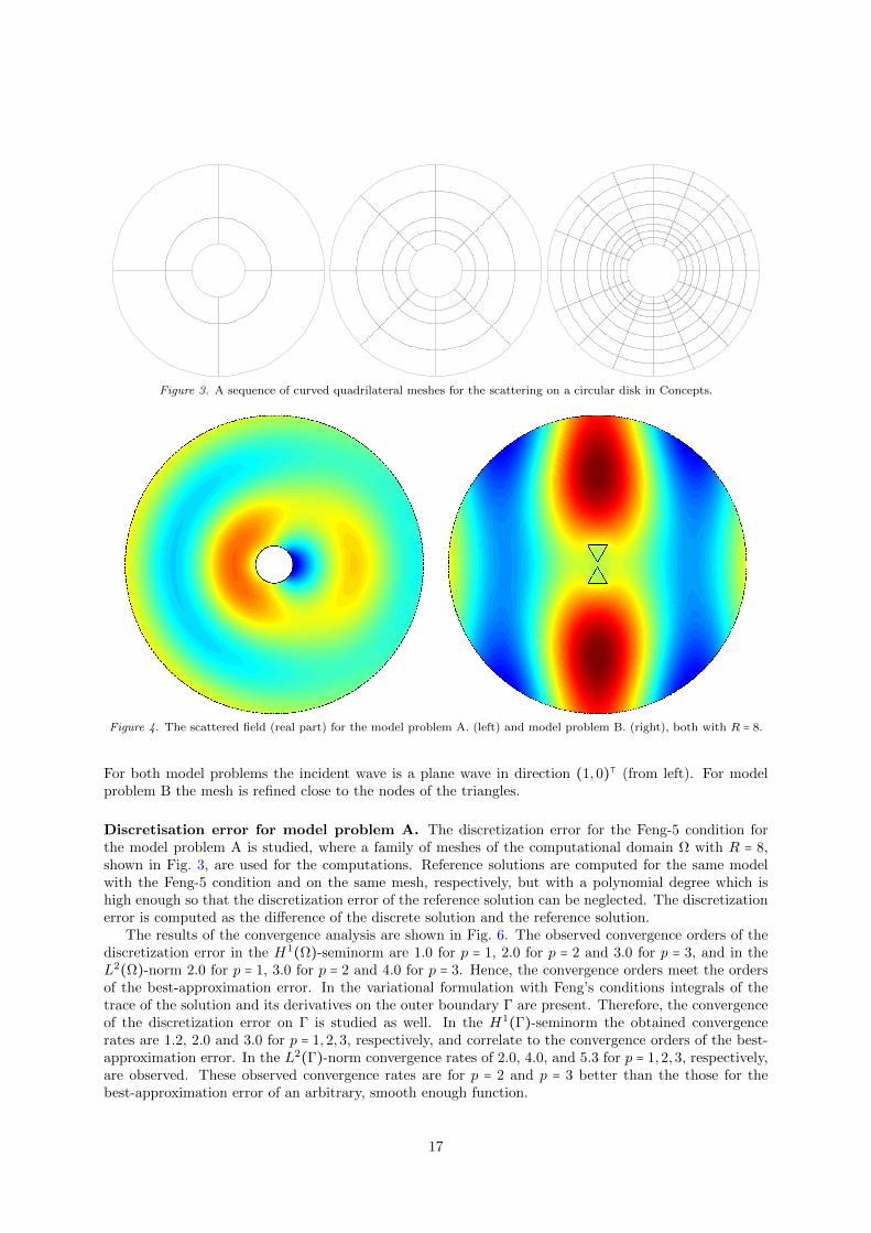
Figure 3. A sequence of curved quadrilateral meshes for the scattering on a circular disk in Concepts.

Figure 4. The scattered field (real part) for the model problem A. (left) and model problem B. (right), both with R = 8.

For both model problems the incident wave is a plane wave in direction (1,0)⊺ (from left). For modelproblem B the mesh is refined close to the nodes of the triangles.

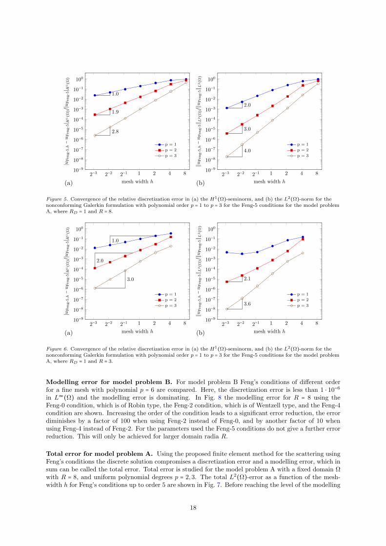
Discretisation error for model problem A. The discretization error for the Feng-5 condition forthe model problem A is studied, where a family of meshes of the computational domain Ω with R = 8,shown in Fig. 3, are used for the computations. Reference solutions are computed for the same modelwith the Feng-5 condition and on the same mesh, respectively, but with a polynomial degree which ishigh enough so that the discretization error of the reference solution can be neglected. The discretizationerror is computed as the difference of the discrete solution and the reference solution.

The results of the convergence analysis are shown in Fig. 6. The observed convergence orders of thediscretization error in the H1(Ω)-seminorm are 1.0 for p = 1, 2.0 for p = 2 and 3.0 for p = 3, and in theL2(Ω)-norm 2.0 for p = 1, 3.0 for p = 2 and 4.0 for p = 3. Hence, the convergence orders meet the ordersof the best-approximation error. In the variational formulation with Feng’s conditions integrals of thetrace of the solution and its derivatives on the outer boundary Γ are present. Therefore, the convergenceof the discretization error on Γ is studied as well. In the H1(Γ)-seminorm the obtained convergencerates are 1.2, 2.0 and 3.0 for p = 1,2,3, respectively, and correlate to the convergence orders of the best-approximation error. In the L2(Γ)-norm convergence rates of 2.0, 4.0, and 5.3 for p = 1,2,3, respectively,are observed. These observed convergence rates are for p = 2 and p = 3 better than the those for thebest-approximation error of an arbitrary, smooth enough function.

17

(a)

2−3 2−2 2−1 1 2 4 810−9

10−8

10−7

10−6

10−5

10−4

10−3

10−2

10−1

100

1.0

1.9

2.8

mesh width h

∣uFeng-5,h−u

Feng-5∣ H

1(Ω)/∣u

Feng-5∣ H

1(Ω)

p = 1

p = 2

p = 3

(b)

2−3 2−2 2−1 1 2 4 810−9

10−8

10−7

10−6

10−5

10−4

10−3

10−2

10−1

100

2.0

3.0

4.0

mesh width h

∥u

Feng-5,h−u

Feng-5∥L

2(Ω)/∥u

Feng-5∥L

2(Ω)

p = 1

p = 2

p = 3

Figure 5. Convergence of the relative discretization error in (a) the H1(Ω)-seminorm, and (b) the L2(Ω)-norm for thenonconforming Galerkin formulation with polynomial order p = 1 to p = 3 for the Feng-5 conditions for the model problemA, where RD = 1 and R = 8.

(a)

2−3 2−2 2−1 1 2 4 810−9

10−8

10−7

10−6

10−5

10−4

10−3

10−2

10−1

100

1.0

2.0

3.0

mesh width h

∣uFeng-5,h−u

Feng-5∣ H

1(Ω)/∣u

Feng-5∣ H

1(Ω)

p = 1

p = 2

p = 3

(b)

2−3 2−2 2−1 1 2 4 810−9

10−8

10−7

10−6

10−5

10−4

10−3

10−2

10−1

100

2.1

3.6

mesh width h

∥u

Feng-5,h−u

Feng-5∥L

2(Ω)/∥u

Feng-5∥L

2(Ω)

p = 1

p = 2

p = 3

Figure 6. Convergence of the relative discretization error in (a) the H1(Ω)-seminorm, and (b) the L2(Ω)-norm for thenonconforming Galerkin formulation with polynomial order p = 1 to p = 3 for the Feng-5 conditions for the model problemA, where RD = 1 and R = 3.

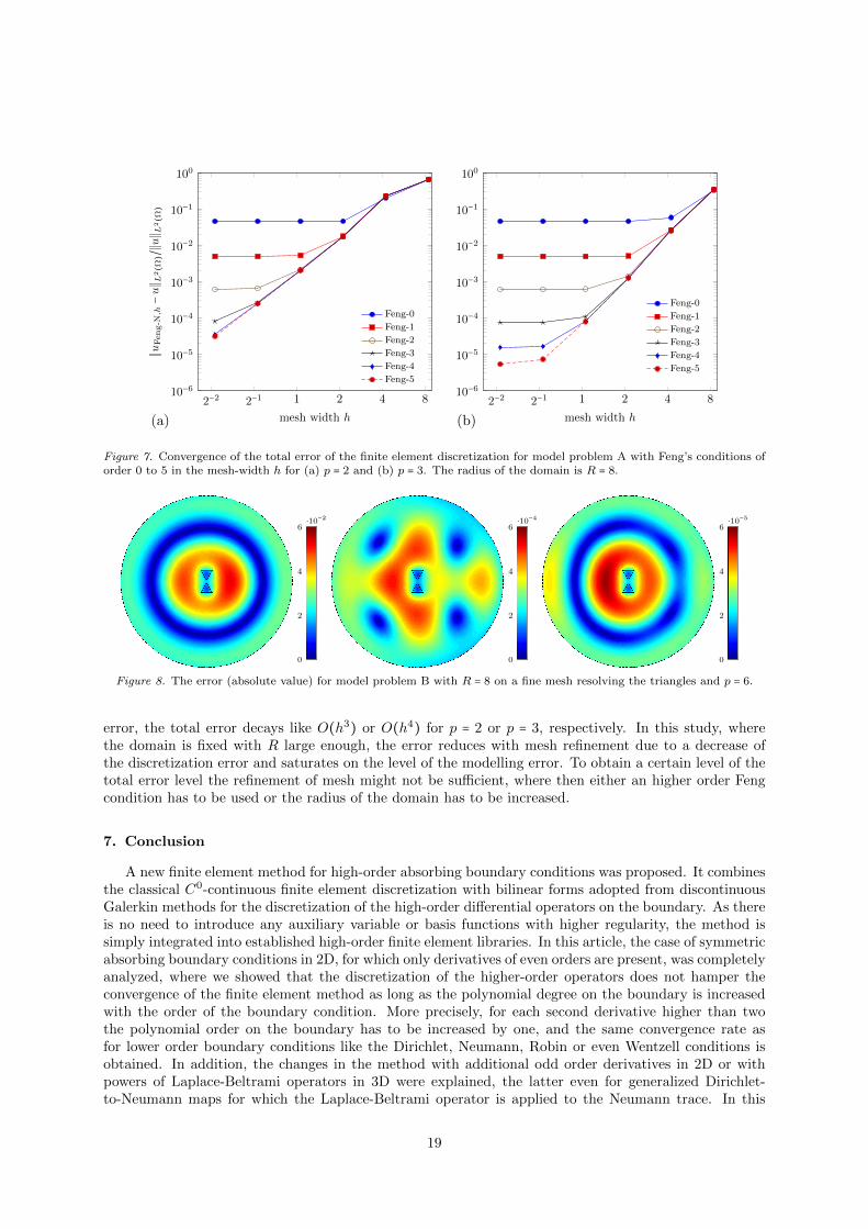
Modelling error for model problem B. For model problem B Feng’s conditions of different orderfor a fine mesh with polynomial p = 6 are compared. Here, the discretization error is less than 1 ⋅ 10−6

in L∞(Ω) and the modelling error is dominating. In Fig. 8 the modelling error for R = 8 using theFeng-0 condition, which is of Robin type, the Feng-2 condition, which is of Wentzell type, and the Feng-4condition are shown. Increasing the order of the condition leads to a significant error reduction, the errordiminishes by a factor of 100 when using Feng-2 instead of Feng-0, and by another factor of 10 whenusing Feng-4 instead of Feng-2. For the parameters used the Feng-5 conditions do not give a further errorreduction. This will only be achieved for larger domain radia R.

Total error for model problem A. Using the proposed finite element method for the scattering usingFeng’s conditions the discrete solution compromises a discretization error and a modelling error, which insum can be called the total error. Total error is studied for the model problem A with a fixed domain Ωwith R = 8, and uniform polynomial degrees p = 2,3. The total L2(Ω)-error as a function of the mesh-width h for Feng’s conditions up to order 5 are shown in Fig. 7. Before reaching the level of the modelling

18

(a)

2−2 2−1 1 2 4 810−6

10−5

10−4

10−3

10−2

10−1

100

mesh width h

∥u

Feng-N,h−u∥L

2(Ω)/∥u∥L

2(Ω)

Feng-0

Feng-1

Feng-2

Feng-3

Feng-4

Feng-5

(b)

2−2 2−1 1 2 4 810−6

10−5

10−4

10−3

10−2

10−1

100

mesh width h

Feng-0

Feng-1

Feng-2

Feng-3

Feng-4

Feng-5

Figure 7. Convergence of the total error of the finite element discretization for model problem A with Feng’s conditions oforder 0 to 5 in the mesh-width h for (a) p = 2 and (b) p = 3. The radius of the domain is R = 8.

0

2

4

6⋅10−2

0

2

4

6⋅10−4

0

2

4

6⋅10−5

Figure 8. The error (absolute value) for model problem B with R = 8 on a fine mesh resolving the triangles and p = 6.

error, the total error decays like O(h3) or O(h4) for p = 2 or p = 3, respectively. In this study, wherethe domain is fixed with R large enough, the error reduces with mesh refinement due to a decrease ofthe discretization error and saturates on the level of the modelling error. To obtain a certain level of thetotal error level the refinement of mesh might not be sufficient, where then either an higher order Fengcondition has to be used or the radius of the domain has to be increased.

7. Conclusion

A new finite element method for high-order absorbing boundary conditions was proposed. It combinesthe classical C0-continuous finite element discretization with bilinear forms adopted from discontinuousGalerkin methods for the discretization of the high-order differential operators on the boundary. As thereis no need to introduce any auxiliary variable or basis functions with higher regularity, the method issimply integrated into established high-order finite element libraries. In this article, the case of symmetricabsorbing boundary conditions in 2D, for which only derivatives of even orders are present, was completelyanalyzed, where we showed that the discretization of the higher-order operators does not hamper theconvergence of the finite element method as long as the polynomial degree on the boundary is increasedwith the order of the boundary condition. More precisely, for each second derivative higher than twothe polynomial order on the boundary has to be increased by one, and the same convergence rate asfor lower order boundary conditions like the Dirichlet, Neumann, Robin or even Wentzell conditions isobtained. In addition, the changes in the method with additional odd order derivatives in 2D or withpowers of Laplace-Beltrami operators in 3D were explained, the latter even for generalized Dirichlet-to-Neumann maps for which the Laplace-Beltrami operator is applied to the Neumann trace. In this

19

way, the method applies to generalized impedance boundary conditions as well as generalized absorbingboundary conditions in 3D such as the BGT conditions. A series of numerical experiments for Feng’sabsorbing boundary conditions up to order five illustrated the applicability of the method and validatesthe theoretically obtained estimates of the discretization error.

Based on C0-continuous finite element spaces, the proposed interior penalty formulation easily handleslocal absorbing boundary conditions of arbitrary order, tangential derivatives on curved boundaries ofvarious shapes and with elements of various types and even locally varying polynomial order, both in 2Dand 3D. As absorbing boundary conditions of higher order, and hence, higher accuracy, exhibit usuallyhigher order derivatives, the proposed numerical method may lead to significantly higher accuracies withthe same discretisation in the domain while only increasing the polynomial order in the boundary edges.

As an extension, the method is straightforwardly combined with discontinuous Galerkin methods,where besides the usual terms on the element boundaries additional terms on the domain boundaryappear already for second derivatives. Note that in this paper only smooth boundaries and smoothcoefficients αj were considered. An extension of the proposed method to boundaries with a corner or tothe case where the coefficients αj are only piecewise smooth is not a trivial task and has to be studiedseparately.

References

[1] Adams, R. A. Sobolev spaces. Academic Press, New-York, London, 1975.

[2] Antoine, X., Barucq, H., and Bendali, A. Bayliss-Turkel-like radiation conditions on surfacesof arbitrary shape. J. Math. Anal. Appl. 229, 1 (1999), 184–211.

[3] Aslanyurek, B., Haddar, H., and Sahinturk, H. Generalized impedance boundary conditionsfor thin dielectric coatings with variable thickness. Wave Motion 48, 7 (2011), 681–700.

[4] Babuska, I., and Osborn, J. Handbook of Numerical Analysis, vol. II. North-Holland, 1991,ch. Eigenvalue Problems, pp. 641–787.

[5] Barucq, H., Djellouli, R., and Saint-Guirons, A. Three-dimensional approximate local DtNboundary conditions for prolate spheroid boundaries. J. Comput. Appl. Math. 234, 6 (2010), 1810 –1816.

[6] Bayliss, A., Gunzburger, M., and Turkel, E. Boundary conditions for the numerical solutionof elliptic equations in exterior regions. SIAM J. Appl. Math. 42, 2 (1982), 430–451.

[7] Bendali, A., and Lemrabet, K. The effect of a thin coating on the scattering of a time-harmonicwave for the Helmholtz equation. SIAM J. Appl. Math. 6 (1996), 1664–1693.

[8] Bonnaillie-Noel, V., Dambrine, M., Herau, F., and Vial, G. On generalized Ventcel’s typeboundary conditions for Laplace operator in a bounded domain. SIAM J. Math. Anal., 42, 2 (2010),931–945.

[9] Brenner, S., and Scott, L. The mathematical theory of finite element methods. Springer-Verlag,New York, 1994.

[10] Brenner, S., and Sung, L.-Y. C0 interior penalty methods for fourth order elliptic boundaryvalue problems on polygonal domains. J. Sci. Comput. 22-23, 1-3 (2005), 83–118.

[11] Ciarlet, P. The Finite Element Method for Elliptic Problems, vol. 4 of Studies in Mathematicsand its Applications. North-Holland, Amsterdam, 1978.

[12] Concepts Development Team. Webpage of Numerical C++ Library Concepts 2.http://www.concepts.math.ethz.ch, 2014.

[13] Delourme, B., Haddar, H., and Joly, P. Approximate models for wave propagation acrossthin periodic interfaces. J. Math. Pures Appl. (9) 98, 1 (2012), 28–71.

20

[14] Engquist, B., and Nedelec, J.-C. Effective boundary conditions for acoustic and electromagneticscattering in thin layers. Tech. rep., Ecole Polytechnique Paris, 1993. Rapport interne du C.M.A.P.

[15] Frauenfelder, P., and Lage, C. Concepts – An Object-Oriented Software Package for PartialDifferential Equations. Math. Model. Numer. Anal. 36, 5 (2002), 937–951.

[16] Givoli, D. Non-reflecting boundary conditions. J. Comput. Phys. 94, 1 (1991), 1–29.

[17] Givoli, D. High-order nonreflecting boundary conditions without high-order derivatives. J. Comput.Phys. 170, 2 (2001), 849–870.

[18] Givoli, D. High-order local non-reflecting boundary conditions: a review. Wave Motion 39, 4(2004), 319–326.

[19] Givoli, D., and Keller, J. B. Special finite elements for use with high-order boundary conditions.Comput. Methods Appl. Mech. Engrg. 119, 3-4 (1994), 199–213.

[20] Givoli, D., Patlashenko, I., and Keller, J. B. High-order boundary conditions and finiteelements for infinite domains. Comput. Methods Appl. Mech. Engrg. 143, 1-2 (1997), 13–39.

[21] Grote, M., Schneebeli, A., and Schotzau, D. Discontinuous Galerkin finite element methodfor the wave equation. SIAM J. Numer. Anal. 44, 6 (2006), 2408–2431.

[22] Haddar, H., Joly, P., and Nguyen, H. Generalized impedance boundary conditions for scatter-ing by strongly absorbing obstacles: the scalar case. Math. Models Methods Appl. Sci 15, 8 (2005),1273–1300.

[23] Hagstrom, T., Mar-Or, A., and Givoli, D. High-order local absorbing conditions for the waveequation: Extensions and improvements. J. Comput. Phys. 227, 6 (2008), 3322 – 3357.

[24] Hagstrom, T., and Warburton, T. A new auxiliary variable formulation of high-order localradiation boundary conditions: corner compatibility conditions and extensions to first-order systems.Wave Motion 39, 4 (2004), 327 – 338.

[25] Harari, I. Computational Methods for Problems of Acoustics with Particular Reference to ExteriorDomains. PhD thesis, Stanford University, Stanford, USA, 1988.

[26] Ihlenburg, F. Finite Element Analysis of Acoustic Scattering. Springer-Verlag, 1998.

[27] Koh, A. L., Fernandez-Domınguez, A. I., McComb, D. W., Maier, S. A., and Yang, J. K.High-resolution mapping of electron-beam-excited plasmon modes in lithographically defined goldnanostructures. Nano Lett. 11, 3 (2011), 1323–1330.

[28] Kozlov, V. A., Maz′ya, V. G., and Rossmann, J. Elliptic boundary value problems in domainswith point singularities, vol. 52 of Mathematical Surveys and Monographs. American MathematicalSociety, Providence, RI, 1997.

[29] Leontovich, M. A. On approximate boundary conditions for electromagnetic fields on the surfaceof highly conducting bodies. In Research in the propagation of radio waves. Academy of Sciences ofthe USSR, Moscow, 1948, pp. 5–12. (In Russian).

[30] Melenk, J. M., and Sauter, S. Wavenumber explicit convergence analysis for Galerkin dis-cretizations of the Helmholtz equation. SIAM J. Numer. Anal. 49, 3 (2011), 1210–1243.

[31] Nedelec, J.-C. Acoustic and Electromagnetic Equations. No. 144 in Applied Mathematical Sci-ences. Springer Verlag, 2001.

[32] Patlashenko, I., and Givoli, D. Non-reflecting finite element schemes for three-dimensionalacoustic waves. J. Comput. Acoust. 5, 1 (1997), 95–115.

21

[33] Poignard, C. Asymptotics for steady-state voltage potentials in a bidimensional highly contrastedmedium with thin layer. Math. Meth. Appl. Sci. 31, 4 (2008), 443–479.

[34] Riviere, B., Wheeler, M. F., and Girault, V. A priori error estimates for finite elementmethods based on discontinuous approximation spaces for elliptic problems. SIAM J. Numer. Anal.39, 3 (2001), 902–931.

[35] Rytov, S. Calculation of skin effect by perturbation method. Zhurnal Experimental’noi I Teo-reticheskoi Fiziki 10 (1940), 180–189.

[36] Sauter, S., and Schwab, C. Boundary element methods. Springer-Verlag, Heidelberg, 2011.

[37] Schatz, A. H. An observation concerning Ritz-Galerkin methods indefinite bilinear forms. Math.Comp. 28 (1974), 959–962.

[38] Schmidt, K., and Chernov, A. A unified analysis of transmission conditions for thin conductingsheets in the time-harmonic eddy current model. SIAM J. Appl. Math. 73, 6 (2013), 1980–2003.

[39] Schmidt, K., and Heier, C. An analysis of Feng’s and other symmetric local absorbing boundaryconditions. ESAIM: Math. Model. Numer. Anal. 49, 1 (2015), 257–273.

[40] Schmidt, K., and Kauf, P. Computation of the band structure of two-dimensional photoniccrystals with hp finite elements. Comp. Meth. App. Mech. Engr. 198 (2009), 1249–1259.

[41] Schmidt, K., and Thons-Zueva, A. Impedance boundary conditions for acoustic time harmonicwave propagation in viscous gases. Submitted to Math. Meth. Appl. Sci.

[42] Schwab, C. p- and hp-finite element methods: Theory and applications in solid and fluid mechanics.Oxford University Press, Oxford, UK, 1998.

[43] Senior, T. Impedance boundary conditions for imperfectly conducting surfaces. Appl. Sci. Res.8(B), 1 (1960), 418–436.

[44] Senior, T., and Volakis, J. Approximate Boundary Conditions in Electromagnetics. Institutionof Electrical Engineers, 1995.

[45] Senior, T. B. A. Generalized boundary and transition conditions and the question of uniqueness.Radio Sci. 27, 6 (1992), 929–934.

[46] Sun, S., and Wheeler, M. F. Symmetric and nonsymmetric discontinuous Galerkin methods forreactive transport in porous media. SIAM J. Numer. Anal. 43, 1 (2005), 195–219.

[47] Wang, M., Engstrom, C., Schmidt, K., and Hafner, C. On high-order FEM applied tocanonical scattering problems in plasmonics. J. Comput. Theor. Nanosci. 8 (2011), 1–9.

[48] Warburton, T., and Hesthaven, J. S. On the constants in hp-finite element trace inverseinequalities. Comput. Methods Appl. Mech. Engrg., 192 (2003), 2765–2773.

[49] Wheeler, M. F. An elliptic collocation-finite element method with interior penalties. SIAM J.Numer. Anal. 15, 1 (1978), 152–161.

[50] Yuferev, S., and Di Rienzo, L. Surface impedance boundary conditions in terms of variousformalisms. IEEE Trans. Magn. 46, 9 (Sept 2010), 3617–3628.

[51] Yuferev, S., and Ida, N. Surface Impedance Boundary Conditions: A Comprehensive Approach.CRC Press, 2010.

22