T E C H N I C A L R E P O R T 0 3 8

2 0 0 7

Ministry of Forests and Range Forest Science Program

A Framework to Support Landscape Analyses

of Habitat Supply and Effects on Populations

of Forest-dwelling Species: A Case Study

Based on the Northern Spotted Owl

Ministry of Forests and RangeForest Science Program

A Framework to Support Landscape Analyses of Habitat Supply and Effects on Populations of Forest-dwelling Species: A Case Study Based on the Northern Spotted Owl

G.D. Sutherland, D.T. O’Brien, S.A. Fall, F.L. Waterhouse,

A.S. Harestad, and J.B. Buchanan (editors)

The use of trade, firm, or corporation names in this publication is for the information and convenience of the reader. Such use does not constitute an official endorsement or approval by the Government of British Columbia of any product or service to the exclusion of any others that may also be suitable. Contents of this report are presented for discussion purposes only. Funding assistance does not imply endorsement of any statements or information contained herein by the Government of British Columbia. Uniform Resource Locators (urls), addresses, and contact information contained in this document are current at the time of printing unless otherwise noted.

CitationSutherland, G.D., D.T. O'Brien, S.A. Fall, F.L. Waterhouse, A.S. Harestad, and J.B. Buchanan (editors). 2007. A framework to support landscape analyses of habitat supply and effects on populations of forest-dwelling species: a case study based on the Northern Spotted Owl. B.C. Min. For. Range, Res. Br., Victoria, B.C. Tech. Rep. 038. <http://www.for.gov.bc.ca/hfd/pubs/Docs/Tr/Tr038.htm>

Compiled and edited by

Library and Archives Canada Cataloguing in Publication DataMain entry under title:A framework to support landscape analyses of habitat supply and effects on populations of forest-dwelling species : a case study based on the Northern Spotted Owl(Technical report ; 038)“This project was completed through the co-operative effort of the Canadian Spotted Owl Recovery Team (CSORT) in contract with Cortex Consultants Inc. and Gowlland Technologies Ltd.”--Acknowledgements.Includes bibliographical references: p.

ISBN 978-0-7726-5677-3

. Spotted owl - Effect of habitat modification on - British Columbia - Simulation methods. 2. Spotted owl - Population viability analysis - British Columbia. 3. Spotted owl - Population viability analysis - British Columbia - Simulation methods. 4. Spotted owl - Habitat - British Columbia. 5. Spotted owl - Ecology - British Columbia. 6. Forest management - Environmen-tal aspects - British Columbia. 7. Forest landscape management - British Columbia - Planning. 8. Wildlife recovery - British Columbia. I. Sutherland, Glenn D. (Glenn Douglas), 956- . II. British Columbia. Forest Science Program. III. Canadian Spotted Owl Recovery Team. IV. Cortex Consultants Inc. V. Gowlland Technologies Ltd. VI. Series: Technical report (British Columbia. Forest Science Program) ; 38.

QL696.S83F75 2007 639.97’897 C2007-96009-0

Prepared forB.C. Ministry of Forests and RangeResearch Branch Victoria, BC v8w 9c2

© 2007 Province of British Columbia

Copies of this report may be obtained, depending upon supply, from:Government PublicationsPO Box 9452 Stn Prov GovtVictoria, BC v8w 9v7-800-663-605http://www.publications.gov.bc.ca

For more information on Forest Science Program publications, visit our web site at: <http://www.for.gov.bc.ca/scripts/hfd/pubs/hfdcatalog/index.asp>

G.D. Sutherland, D.T. O’BrienCortex Consultants Inc.Suite 2a-28 Langley StreetVictoria, BC V8W W2gsutherland@cortex.ca, dobrien@cortex.ca

S.A. FallGowlland Technologies Ltd.220 Old Mossy RoadVictoria, BC V9E 2A3andrew@gowlland.ca

F.L. WaterhouseB.C. Ministry of Forests and RangeCoast Forest Region200 Labieux Road Nanaimo, BC V9T 6E9Louise.Waterhouse@gov.bc.ca

A.S. Harestad Simon Fraser UniversityDep. of Biological SciencesBurnaby, BC V5A S6harestad@sfu.ca

J.B. Buchanan Washington Dep. of Fish and WildlifeNatural Resources Building Washington Street SE Olympia, WA 9850Buchajbb@dfw.wa.gov

EXECUTIVE SUMMARY

Planning tools and decision-making processes to support sustainable forestry are an integral part of practicing good forest stewardship in British Colum-bia. The challenges when applying stewardship principles are often at their greatest when resource extraction activities and habitats of forest-dependent species overlap. Tools to represent and integrate information about both ecological processes and predicted consequences of forest management activ-ities, and approaches for comparing costs and benefits of both economic and environmental values, are evolving to meet this challenge. In this document we present a spatial modelling framework designed to assist those confront-ing these challenges to sustainable forestry. Users can use this framework as a tool to evaluate hypotheses about the ecological and economic consequences of management strategies. Of particular interest is the capability of the framework to assist in the search for acceptable trade-offs between social and ecological values—a necessary but challenging requirement of meeting good stewardship objectives in natural resource management.

We illustrate application of the framework using an endangered species in British Columbia, the Northern Spotted Owl (Strix occidentalis caurina; SPOW). Our approach was designed to help decision-makers understand the probable roles of currently hypothesized threats to the population in mod-elled experiments conducted within the framework. We developed indicators representing the condition of the landscape, volumes of merchantable timber harvested from the landscape, and several types of indicators representing population-level status of Spotted Owls. The main questions we examined during the evolution of the framework were:

• What is a reasonable recovery goal for the study species (Spotted Owl) expressed as the number of breeding pairs?

• Is habitat loss a continuing threat, and if so, how? • Is habitat recovery possible, and if so, when and where?• Can potential outcomes for both the case study species and socio-

economic values using a suite of potential management policies be demonstrated?

• Is some suitable habitat of better quality than others? Does the definition of suitable habitat need to account for spatial locations of current and potential populations, a concept related to the idea of “critical habitat”?

• Where should we place our species-specific management areas to capital-ize on habitat?

• Can we better understand the relationship between the recovery goal, the current population size, and current habitat amount and configuration?

• Could Barred Owls (Strix varia varia; BDOW) be a significant threat?

To help answer these questions, we developed models for spatial landscape projection, ecological classification, cross-scale habitat assessment, popula-tion dynamics, and reserve selection. The modelling framework used to represent these components is necessarily a simplistic representation of a very complex reality (Walters 986). Sufficient empirical data needed to define functional relationships were not always available. Estimates of parameters, even where data are available, required care in their use and

iii

iv

interpretation. These, combined with informed expert judgements about many key hypotheses and relationships, formed the basis of model building and testing. The following chapters outline the data and assumptions used to model the Spotted Owl, the development of the suite of tools for the frame-work, and the findings on both the model framework and the Spotted Owl as synthesized through the framework.

Section presents an overview of the modelling framework, and describes the six integrated, spatially explicit model components. These are:

. a landscape dynamics model for projecting forest growth and stand-re-placing natural disturbances that is capable of fully spatial timber supply analyses;

2. a habitat supply model that can be tailored for particular species;3. a spatial model for calculating locations of potential territories for a terri-

torial species;4. a structural connectivity model for assessing spatial arrangement and

proximity of habitat, territories, and management areas;5. a spatial population model for projecting population dynamics of a par-

ticular species on projected landscapes; and6. an evaluation post-processor that implements rules for identifying and

ranking potential habitat reserves based on biological and other criteria measured at multiple scales.

Section 2 describes the ecological and management problem of recovery planning for the Spotted Owl that formed the case study we used to develop and test the framework. Evidence indicates that the Spotted Owl population in British Columbia is small and declining. Currently known and potential threats to this species in British Columbia include:

. loss of nesting and/or foraging habitat,2. fragmentation of nesting and/or foraging habitat,3. negative effects from environmental and genetic factors related to small

population sizes,4. competition from Barred Owls,5. climate change, and6. disease.

We used the components of the framework to test a number of ecological hypotheses about the first four of these threats to learn how projected out-comes behave in relation to our assumptions about the causal factors influencing the status of this species.

Sections 3–7 describe the primary ecological modelling components of the framework for projecting future ecological states. The landscape dynamics component (Section 3) combines a spatially explicit forest state model with a stand-replacing natural disturbance model to estimate sustainable harvest flows and to project spatial time-series of forest-state indicators (e.g., stand age, height, structure, disturbances) for a particular “landscape change” sce-nario. The ecological consequences for the case study species (Spotted Owl) of the projected landscape dynamics under each scenario are then assessed using the finest spatial scale (termed site-scale) habitat classification models for foraging, nesting, and movement (Section 4) based on biophysical vari-

v

ables representing the influences of climate, topography, vegetation structure, and composition. We then evaluate habitat at the coarser scale of potential territories (Section 5), searching for those areas where the spatial configura-tion of habitat meet criteria for supporting a breeding site and territory. At a still coarser scale, the spatial proximity and clustering of habitat across the landscape is evaluated using spatial graph techniques for measuring connec-tivity (Section 6). The results at this scale of ecological assessment provide data on the effects of loss of connectivity on individuals or the population, and can also be used to investigate the efficacy of such management options as potential habitat corridors or reserves. In Section 7, we explore the conse-quences of the changing landscape structure upon individuals and the population using an individual-based spatially explicit population model. This model permits systematic study of alternative hypotheses of habitat change, demographic factors (e.g., recruitment, survival), and dispersion of nest sites on potential population trends. It can also be extended to assess effects of other threats (e.g., competition from Barred Owls, climate change).

Sections 8–0 demonstrate the post-processing analyses of indicators produced by each model component to inform decisions on the types of questions involved in recovery planning. Section 8 describes a habitat quality assessment tool built using a Bayesian belief network that weights selected habitat attributes measured at the site, territory, and population scales. It thus obtains an integrated measure of biological habitat quality for each spatial lo-cation that is deemed to be “suitable habitat.” This habitat quality evaluation can be used to facilitate selection of critical habitat locations for the study species. In Section 9, we advance this concept further by using a resource lo-cation model that selects candidate habitat reserve areas that meet biological and/or risk criteria for recovery goals at different times in the future. This ap-proach is particularly useful for land-use planning problems involving species conservation because it facilitates efficient selection of habitat that meets both current and future biological goals for the amount and spatial configuration of habitat and other biological criteria while minimizing im-pacts on other values. In Section 0, we illustrate how to apply the outputs of the framework to evaluate different policy options for forest and species management, and compare their ecological and economic costs and benefits.

Finally, in Section we: () summarize the strengths and weaknesses of the design and implementation of the framework for spatial projections of large-scale ecological and management problems such as those found in re-covery planning; and (2) present key findings for the current population, future population, habitat management for recovery, and habitat require-ments derived for the Spotted Owl case study. This case study species is of significant conservation concern in Canada and in British Columbia as well as elsewhere in the Pacific Northwest; thus our findings are of interest well beyond simply demonstrating analytical and modelling approaches. The find-ings of the research must be considered collectively, as they apply to the issues of recovery of this species in British Columbia.

We conclude by noting that several aspects of the resulting framework build upon and extend previously developed model approaches and concepts. Our design approach of separating the main ecological, management, and analysis components of the system into relatively autonomous components (e.g., timber supply analysis, landscape dynamics, habitat supply, territory analysis, connectivity analysis, and population dynamics) allowed us to

vi

efficiently and rigorously explore different hypotheses about the causes of declines in Spotted Owl populations. In turn, careful design of modelling ex-periments allowed us to elucidate the relative influences of different factors (habitat, management, demographics) on recovery options. Looking beyond the specific analyses undertaken in a particular study or the conclusions drawn from the results, we believe that a substantial benefit of this project was the process formulated to develop the framework, which promoted com-munication and learning among stakeholders about the intricacies of a complex and difficult resource management problem.

We are (and must be) fairly conservative in our interpretation of the find-ings obtained with the framework in our case study. From the outset, we did not expect spatial modelling results alone to provide a complete solution for recovery of either the British Columbia Spotted Owl population or indeed any species, because of uncertainties in biological parameters, in inventory data, and in describing and projecting all possible threats to populations. We argue that the structure of the framework is very amenable to further inform-ing (and being informed by) long-term monitoring programs for recovering species designed to assess management strategies established to promote the chances of recovering an endangered species or population.

ACKNOWLEDGEMENTS

This project was completed through the co-operative effort of the Canadian Spotted Owl Recovery Team (CSORT)1 in contract with Cortex Consultants Inc. and Gowlland Technologies Ltd. All CSORT members reviewed and con-tributed to project development at various stages. In particular, we would like to thank the research sub-group of the CSORT for their time and efforts to improve the modelling. All members of the CSORT willingly made their unpublished data available and enthusiastically discussed ideas at length, without which this research project would not have been possible. Interpreta-tions of the findings in this document do not necessarily reflect the opinions of any one individual or organization.

Members of the CSORT and external stakeholders reviewed and comment-ed on various interim results. Don Morgan, Brian Nyberg, Doug Steventon, Christine Fletcher (all of B.C. Ministry of Forests and Range; MOFR), Peter Arcese (University of British Columbia), and Bruce Marcot (USDA Forest Service) reviewed scientific and technical aspects of this document and con-siderably improved its clarity. Peter Ott, Del Meidinger, Geoff Cushon, Denis Collins (all of MOFR), and Andrew Howard (Cortex Consultants Inc.) also constructively reviewed this document in whole or in part. Other data and ideas were provided by Eric Forsman (U.S. Department of Agriculture Forest Service and Oregon State University). Cortex Consultants Inc. assembled the data, with assistance from Jeff Stone (Southern Interior Forest Region, MOFR), Insha Khan (B.C. Integrated Land Management Bureau; ILMB, [pre-viously Sustainable Resource Management]), Brigitte Dorner, and Bob Gray (RW Gray Consulting Ltd.). Notes and minutes of workshops and project-re-lated meetings were taken by Kym Welstead and Susan Leech (FORREX).

The projects forming the basis for this document benefited from substan-tial previous research and development work, and past input and collabora-tion on some of the model components is acknowledged from Marvin Eng and Don Morgan (Research Branch, MOFR), Tim Bogle and Dave Waddell (Forest Analysis and Inventory Branch, MOFR), Marie-Josée Fortin (Univer-sity of Toronto), and Micheline Manseau (Parks Canada).

Funding for these projects was provided by several project partners and co-operators. We gratefully acknowledge the financial support provided by: International Forest Products Ltd. through their Forest Innovation Agree-ment; the Forest Science Program under Forestry Innovation Investment Ltd. of B.C.; Provincial support by the Ministries of Forests and Range, Agricul-ture and Lands (MAL, previously Sustainable Resource Management, now including the B.C. Species at Risk Coordination Office), and Environment (MOE); and Federal support by the Canadian Wildlife Service, Environment Canada, and the Coast Forest Products Association. Assistance from John Deal of Canadian Forest Products Ltd. helped make this publication possible. The final report was copy-edited by Jodie Krakowski and typeset by Donna Lindenberg, Newport Bay Publishing Limited. Publication production was coordinated by Paul Nystedt and Rick Scharf. To all, our thanks.

vii

Regular and Alternate members: Myke Chutter (Chair), MOE; Ian Blackburn, MOE; Derek Bonin, Greater Vancouver Regional District; Joe Buchanan, Washington Department of Fish and Wildlife; David Cunnington, Canadian Wildlife Service; Leonard Feldes, B.C. Timber Sales; Alton Harestad, Simon Fraser University; Trish Hayes, Canadian Wildlife Service; Don Heppner, MOFR; Les Kiss, Coast Forest Products Association; John Surgenor, MOE; Wayne Wall, International Forest Products Ltd.; F. Louise Waterhouse, MOFR; Liz Williams, mal.

TABLE OF CONTENTS

viii

Executive Summary . . . . . . . . . . . . . . . . . . . . . . . . . . . . . . . . . . . . . . . . . . . . . . iiiAcknowledgements . . . . . . . . . . . . . . . . . . . . . . . . . . . . . . . . . . . . . . . . . . . . . . viiList of Contributors . . . . . . . . . . . . . . . . . . . . . . . . . . . . . . . . . . . . . . . . . . . . . . xiii Overview of the Landscape Analysis Framework . . . . . . . . . . . . . . . . .

. Introduction . . . . . . . . . . . . . . . . . . . . . . . . . . . . . . . . . . . . . . . . . . . . . . .2 Objectives . . . . . . . . . . . . . . . . . . . . . . . . . . . . . . . . . . . . . . . . . . . . . . . . 2.3 Components of the Framework . . . . . . . . . . . . . . . . . . . . . . . . . . . . . 3.4 Implementation of the Framework . . . . . . . . . . . . . . . . . . . . . . . . . . . 5

2 Case Study: Supporting Recovery Planning for the Northern Spotted Owl in British Columbia . . . . . . . . . . . . . . . . . . . . . . 62. Ecological Background . . . . . . . . . . . . . . . . . . . . . . . . . . . . . . . . . . . . . 6

2.. Distribution and population trends . . . . . . . . . . . . . . . . . . . . . 62..2 Stand- and landscape-level characteristics

of Spotted Owl habitat . . . . . . . . . . . . . . . . . . . . . . . . . . . . . . . . 72.2 Process of Recovery Planning for the Northern Spotted Owl . . . . 72.3 Scope of the Modelling . . . . . . . . . . . . . . . . . . . . . . . . . . . . . . . . . . . . . 8

2.3. Study area . . . . . . . . . . . . . . . . . . . . . . . . . . . . . . . . . . . . . . . . . . . 82.3.2 Spatial and temporal scope of the case study . . . . . . . . . . . . . 8

3 Landscape Projection Component . . . . . . . . . . . . . . . . . . . . . . . . . . . . . 93. Spatially Explicit Timber Supply Model . . . . . . . . . . . . . . . . . . . . . . 03.2 Natural Disturbance Dynamics . . . . . . . . . . . . . . . . . . . . . . . . . . . . . 3.3 Application of the Landscape Dynamics Model to

Estimate Harvest Flows within the Spotted Owl Range . . . . . . . . . 23.3. Methods . . . . . . . . . . . . . . . . . . . . . . . . . . . . . . . . . . . . . . . . . . . . 23.3.2 Results and discussion . . . . . . . . . . . . . . . . . . . . . . . . . . . . . . . . 3

4 Base Habitat Classification at the Site Scale . . . . . . . . . . . . . . . . . . . . . . 44. Types of Habitats Classified . . . . . . . . . . . . . . . . . . . . . . . . . . . . . . . . . 5

4.. Application of site-scale base habitat classification in the case study: nesting and foraging habitat . . . . . . . . . . . . 6

4.2 Least-cost Model for Movement and Dispersal Habitat Classification . . . . . . . . . . . . . . . . . . . . . . . . . . . . . . . . . . . . . . 7

5 Habitat Evaluation Component for Territory-scale Analysis . . . . . . . 25. Estimation of Potential Nest Sites and Application

in the Case Study . . . . . . . . . . . . . . . . . . . . . . . . . . . . . . . . . . . . . . . . . . 25.2 Estimation of Maximum Number of Territories in the

Case Study . . . . . . . . . . . . . . . . . . . . . . . . . . . . . . . . . . . . . . . . . . . . . . . 225.2. Implementation of the maximum territories model

in the case study . . . . . . . . . . . . . . . . . . . . . . . . . . . . . . . . . . . . . 235.2.2 Application of the maximum territories model in

the Spotted Owl case study . . . . . . . . . . . . . . . . . . . . . . . . . . . . 24

ix

6 Estimating Structural and Functional Connectivity Using the Framework . . . . . . . . . . . . . . . . . . . . . . . . . . . . . . . . . . . . . . . . . 276. Fundamental Definitions and Methodology for

Estimating Connectivity Using Spatial Graphs . . . . . . . . . . . . . . . . 286.2 Application of the Structural Connectivity

Approach to Identify Centres of Habitat . . . . . . . . . . . . . . . . . . . . . . 296.3 Application of the Structural Connectivity

Approach to Identify Potential Corridors . . . . . . . . . . . . . . . . . . . . . 337 Population Evaluation Component . . . . . . . . . . . . . . . . . . . . . . . . . . . . . 35

7. General Description of the Individual-based Population Model . . 357.. Life stages and population structure . . . . . . . . . . . . . . . . . . . . 367..2 Population dynamics . . . . . . . . . . . . . . . . . . . . . . . . . . . . . . . . . 37

7.2 Application of the Population Model in the Case Study . . . . . . . . . 427.2. Calibration of population vital rates . . . . . . . . . . . . . . . . . . . . 427.2.2 Indicators of population status and trends . . . . . . . . . . . . . . . 43

7.3 Exploring Interactions between Land Management Policies and Population Size . . . . . . . . . . . . . . . . . . . . . . . . . . . . . . . . 44

7.4 Exploring Potential Northern Barred Owl Effects with the Population Model . . . . . . . . . . . . . . . . . . . . . . . . . . . . . . . . . . . . . . 47

8 Evaluating Current and Future Habitat Quality Using a Bayesian Belief Network . . . . . . . . . . . . . . . . . . . . . . . . . . . . . . . 498. General Description of the Habitat-quality BBN . . . . . . . . . . . . . . . 508.2 Alternative Definitions of Centroids in the BBN . . . . . . . . . . . . . . . 58.3 Application of the Habitat-quality BBN to Identify

High-quality Habitats for Recovery Planning . . . . . . . . . . . . . . . . . . 528.3. Specifying the habitat quality BBN . . . . . . . . . . . . . . . . . . . . . . 528.3.2 Exploring results using the habitat quality BBN . . . . . . . . . . . 60

9 The Resource Location Model for Identifying Critical and Potential Habitat Areas . . . . . . . . . . . . . . . . . . . . . . . . . . . . 609. Basic Definitions and Methodology for Identifying

Resource Units . . . . . . . . . . . . . . . . . . . . . . . . . . . . . . . . . . . . . . . . . . . . 629.2 Application of the RLM to Identify Candidate

Habitat Reserves for Recovery Planning . . . . . . . . . . . . . . . . . . . . . . 649.2. Methods . . . . . . . . . . . . . . . . . . . . . . . . . . . . . . . . . . . . . . . . . . . . 649.2.2 Results and discussion . . . . . . . . . . . . . . . . . . . . . . . . . . . . . . . . 67

0 Assessing Effects of Alternative Land Management Policies Using the Framework . . . . . . . . . . . . . . . . . . . . . . . . . . . . . . . . . . 70. Application of the Framework to Assess Relative Impacts

of Alternative Management Options on Economic and Ecological Indicators . . . . . . . . . . . . . . . . . . . . . . . . . . . . . . . . . . . . . . . 70.. Design of management alternatives . . . . . . . . . . . . . . . . . . . . . 70..2 Evaluating outcomes using relative benefit

trade-off curves . . . . . . . . . . . . . . . . . . . . . . . . . . . . . . . . . . . . . . 73 Summary of the Framework and Case Study Results . . . . . . . . . . . . . . 77

. Summary of the Framework Design . . . . . . . . . . . . . . . . . . . . . . . . . . 77.2 Summary Findings from Application of the

Framework to the Case Study . . . . . . . . . . . . . . . . . . . . . . . . . . . . . . . 79.2. Limitations of case study research findings . . . . . . . . . . . . . . 82

2 Literature Cited . . . . . . . . . . . . . . . . . . . . . . . . . . . . . . . . . . . . . . . . . . . . . . . . 84

x

appendices

Data Sources Used in the Case Study . . . . . . . . . . . . . . . . . . . . . . . . . . . . . 93 2 Definitions and Methodology for Projecting Landscape Dynamics . . . 94 3 Habitat Definitions for the Spotted Owl Case Study . . . . . . . . . . . . . . . . 03 4 Use of Connectivity Analyses for Estimating Proximities of

Known Breeding Sites to Concentrations of Nesting Habitat . . . . . . . . . 8 5 Simulation Experiments to Investigate Hypotheses about the

Spotted Owl . . . . . . . . . . . . . . . . . . . . . . . . . . . . . . . . . . . . . . . . . . . . . . . . . 20 6 Conceptual Approach for Analysis of Land Management Policies . . . . 23 7 Commonly Used Acronyms . . . . . . . . . . . . . . . . . . . . . . . . . . . . . . . . . . . . 28

tables

Description of habitat parameters for maritime, submaritime, and continental ecosystems for stands classified as “structure present” or “structure absent” . . . . . . . . . . . . . . . . . . . . . . . . . . . . . . . . . . . 8

2 Rules for calculating relative costs for Spotted Owl to disperse through a cell type for cost units do not have an exact Euclidean distance equivalent . . . . . . . . . . . . . . . . . . . . . . . . . . . . . . . . . . . 20

3 Parameters and default values for specifying the extent and arrangement of Spotted Owl breeding pair territories . . . . . . . . . . . . . . 23

4 Key differences between conventional and spatial graphs . . . . . . . . . . . 29 5 Description and rules for each Spotted Owl life stage as defined

in the population model . . . . . . . . . . . . . . . . . . . . . . . . . . . . . . . . . . . . . . . . 37 6 Parameters specifying vital rates and behaviour for the British

Columbia Spotted Owl population taken directly or calculated from the listed sources . . . . . . . . . . . . . . . . . . . . . . . . . . . . . . . . . . . . . . . . 40

7 Selected calibrated vital rates for a stable-state population of Spotted Owls on a long-term equilibrium landscape . . . . . . . . . . . . . . . 42

8 Alternative sets of assumptions for the factorial simulation experiments partitioning effects of main factors affecting short-term modelled population trends . . . . . . . . . . . . . . . . . . . . . . . . . . 45

9 Main user-defined nodes and their weightings for ranking habitat quality in the bbn used in the case study . . . . . . . . . . . . . . . . . . . . . . . . . 54

0 The set of evaluation criteria and individual attributes tracked by the RLM through time for each candidate RU in the case study . . . . . . 65

The two sets of criteria and the relative weights applied to each attribute used in this application of the rlm . . . . . . . . . . . . . . . . . 65

2 Representation of the top 25 rus selected by the two sets of criteria, including the numbers of rus and total area in each subregion . . . . . . 70

3 Within-subregion comparisons of percentages of selected attributes contained in the top 25 rus as selected by the two sets of criteria to help interpret the influence of each criterion . . . . . . . . . . . . . . . . . . . . 7

4 Detailed description of policy scenarios assessed based on four factors: Spotted Owl management areas, harvest policy in Spotted Owl management areas, corridor management, and other habitat protection . . . . . . . . . . . . . . . . . . . . . . . . . . . . . . . . . . . . . . . . 72

xi

figures

Conceptual components of the landscape dynamics–habitat–species system showing the main links and feedbacks between components . . . 3

2 Overview of the analysis framework . . . . . . . . . . . . . . . . . . . . . . . . . . . . . 4 3 Implementation of the modelling components of the analysis

framework as a “pipeline” . . . . . . . . . . . . . . . . . . . . . . . . . . . . . . . . . . . . . . 4 4 Study area and management units used in the case study . . . . . . . . . . . . 9 5 Conceptual structure of the spatially explicit timber supply model . . . 6 Realized harvest flows for two selected policies for the four main

management units and their total within the Spotted Owl range . . . . . 4 7 Map showing the current locations of suitable and capable habitat

types within the Spotted Owl range . . . . . . . . . . . . . . . . . . . . . . . . . . . . . . 7 8 Schematic diagram showing the identification of a potential

nest site in the territory evaluation component of the case study . . . . . 22 9 Distribution of potential territories across the Spotted Owl range as

found by one iteration of the maximum territories model . . . . . . . . . . . 26 0 Number of packed territories found in each ecological subregion

by the maximum territories model under the “AgingOnly” land management scenario . . . . . . . . . . . . . . . . . . . . . . . . . . . . . . . . . . . . . 27

Conceptual minimum planar graph for a set of nodes using Euclidean cost . . . . . . . . . . . . . . . . . . . . . . . . . . . . . . . . . . . . . . . . . . . . . . . . 29

2 Illustration of the difference between straight-line and least-cost paths linking nodes . . . . . . . . . . . . . . . . . . . . . . . . . . . . . . . . . . . . . . . . . . . . 30

3 Candidate nesting habitat patches and the mpg of least-cost paths linking nodes for the study area . . . . . . . . . . . . . . . . . . . . . . . . . . . . . . . . . 30

4 An example of a well-connected cluster of nesting habitat patches within the study area meeting all ecological criteria used by the graph-pruning steps . . . . . . . . . . . . . . . . . . . . . . . . . . . . . . . . . . . . . . . . . . . 32

5 The spatial cost relationship between habitat patches and the identified source habitat cluster in the same area as Figure 4 . . . . . . . 32

6 Potential Spotted Owl management corridors connecting current Spotted Owl management units, based on spatial graph analysis overlaid on the digital elevation layer for the base study region . . . . . . 34

7 Diagram representing life stages and transitions in the population model . . . . . . . . . . . . . . . . . . . . . . . . . . . . . . . . . . . . . . . . . . . . . 36

8 Interpolated linear function for estimating breeding adult survival . . . 39 9 Potential effects of initial model population size, land management

scenario, and starting year on short-term trends in modelled populations . . . . . . . . . . . . . . . . . . . . . . . . . . . . . . . . . . . . . . . . . . . . . . . . . . 46

20 Potential effect of displacement of Spotted Owl breeding pairs by Barred Owl projected population sizes . . . . . . . . . . . . . . . . . . . . . . . . . . . 49

2 A conceptual structure of the bbn developed for ranking habitat quality for each cell using outputs from other components of the framework and weighting rules specified within the bbn . . . . . . . . . . . 5

xii

22 The full habitat quality bbn as implemented in the framework for the Spotted Owl case study . . . . . . . . . . . . . . . . . . . . . . . . . . . . . . . . . . 53

23 The integrated habitat quality map at year 0 for the two assumptions of distribution of nesting habitat quality in the case study . . . . . . . . . . . 58

24 The integrated habitat quality map at year 50 for the two assumptions of distribution of nesting habitat quality in the case study . . . . . . . . . . . 59

25 Conceptual diagram of the rlm’s components, main inputs and outputs, and logic flow. . . . . . . . . . . . . . . . . . . . . . . . . . . . . . . . . . . . . . . . . . 63

26 Map of the locations of all possible candidate Resource Units identified by year 50 for the case study, in decreasing order of their integrated habitat quality at year 50 . . . . . . . . . . . . . . . . . . . . . . . . . 67

27 Maps showing the candidate Resource Units for the case study selected according to two sets of policy criteria . . . . . . . . . . . . . . . . . . . . 69

28 Relative changes in short-term and long-term timber supply and Spotted Owl habitat supply trade-off curves for five example management policy scenarios . . . . . . . . . . . . . . . . . . . . . . . . . . . . . . . . . . . 74

29 Relative changes in short-term and long-term timber supply and Spotted Owl potential territory trade-off curves for five example management policy scenarios . . . . . . . . . . . . . . . . . . . . . . . . . . . . . . . . . . . 75

30 Relative trend in the mean population trajectory over the short and long term compared with relative timber supply impacts . . . . . . . . 76

xiii

LIST OF CONTRIBUTORS

Project ManagersLouise Waterhouse B.C. Ministry of Forests and RangeMSc, RPF, RPBio Coast Forest Region 200 Labieux Road Nanaimo, BC V9T 6E9Glenn Sutherland Cortex Consultants Inc.PhD, RPBio Suite 2a-28 Langley Street Victoria, BC V8W W2

Systems Analysts and Topic ExpertsGlenn Sutherland Cortex Consultants Inc.PhD, RPBio Suite 2a-28 Langley Street Victoria, BC V8W W2Daniel O’Brien Cortex Consultants Inc.MSc, RPBio Suite 2a-28 Langley Street Victoria, BC V8W W2Andrew Fall Gowlland Technologies Ltd.PhD 220 Old Mossy Road Victoria, BC V9E 2A3

Topic ExpertsIan Blackburn B.C. Ministry of EnvironmentBSc, RPBio Fish and Wildlife Section 0470 52 Street Surrey, BC V3R 0Y3Joseph Buchanan Washington Department of Fish and WildlifeMSc Natural Resources Building Washington Street SE Olympia, WA 9850David Cunnington Canadian Wildlife Service, Environment CanadaMSc Pacific Wildlife Research Centre 542 Robertson Road Delta, BC V4K 3N2Christine Fletcher B.C. Ministry of Forests and RangeMRM, RPF Forest Analysis and Inventory Branch 520 Blanshard Street Victoria, BC V8W 3J9Alton Harestad Simon Fraser UniversityPhD, RPBio Department of Biological Sciences Burnaby, BC V5A S6Jared Hobbs B.C. Ministry of EnvironmentBSc, RPBio Conservation Planning Section 2975 Jutland Road Victoria, BC V8T 5J9

xiv

Wayne Wall International Forest Products Ltd.RPBio 3-80 Ironwood Road Campbell River, BC V9W 5P7Louise Waterhouse B.C. Ministry of Forests and RangeMSc, RPF, RPBio Coast Forest Region 200 Labieux Road Nanaimo, BC V9T 6E9Liz Williams B.C. Ministry of Agriculture and LandsBSc, Dip Ed, RPBio Species at Risk Coordination Office 780 Blanshard Street Victoria, BC V8W 2H

1 OVERVIEW OF THE LANDSCAPE ANALYSIS FRAMEWORK

1.1 Introduction

Management of forest lands involves potentially conflicting goals between resource managers and the public in British Columbia: () maintaining flows of products from forests that provide economic and other benefits to com-munities and regions, and (2) sustaining biodiversity and other ecological values in those same forests (Bunnell et al. 999). We use the term “biodiver-sity” as referring to all species—including those at risk—as well as ecosystems and ecosystem functions. While there is evidence that good management practices can likely sustain long-term production of wood products and asso-ciated economic opportunities (e.g., Weetman 998), there is also evidence that landscape-level applications of some forest practices do not permit the long-term maintenance of forest-dwelling species (Spies et al. 988; Morrison and Raphael 993). Reconciling different goals in both the short and long term has been the aim of many planning initiatives by different levels of gov-ernment and stakeholders. Tools to represent and integrate information about ecological processes, predicted consequences of management activities, and costs and benefits for economies and biodiversity are evolving to meet this challenge. This document outlines one such new tool—a general land-scape-level modelling framework for analysis of resource management and habitat and population problems using as a case study the Northern Spotted Owl (Strix occidentalis caurina; SPOW).

Ecological models and related decision-support frameworks are simplify-ing abstractions of reality (Jones et al. 20022). They provide structure to what we know and identify what we need to know about a system of interest, such as the ecological and anthropogenic interactions between resource extraction, and the habitats and populations of species. Landscape management (policy) scenarios, habitat suitability criteria, and population characteristics are de-fined as inputs into a modelling framework, while timber volumes harvested (timber supply), amounts of habitat for nesting, foraging, and dispersal (habi-tat supply), and population trend indicators are outputs of the component models in the framework. A modelling framework, therefore, enables the end-user to rank the outcomes of alternative landscape management scenarios relative to one another. Further interpretations of the rankings are then made by the end-users in a decision process that is external to the framework.

The framework we present conceptually follows Jones et al. (2002)3 and includes a number of innovative components to develop landscape scenarios (i.e., a Bayesian belief network [BBN] to assess functional habitat quality at multiple scales, a resource location model [RLM] for reserve selection). Gen-eral habitat concepts have been defined by many authors (e.g., Block and Brennan 993). In the context of this framework, criteria for defining habitat states and types include the composition, structure, and arrangement of the biophysical components of a particular landbase that is used by an individual species at different, nested scales for its survival, reproduction, and dispersal. In the framework, the key scales are: the site scale, the territory scale, and the population scale. The site scale focuses on the attributes of individual cells

2 Jones, R.K., R. Ellis, R. Holt, B. MacArthur, and G. Utzig. 2002. A strategy for habitat supply modelling for British Columbia. Draft Volume . Final project report. Prepared for the Habitat Modelling Steering Committee, B.C. Min. Water, Land and Air Protection, Victoria, B.C. Unpublished report.

3 Ibid.

2

(the smallest unit of land spatially represented in the model; see Section 2.3.2) and its neighbours, which collectively represent a forest stand.4 The site scale is nested within the coarser territory scale, which is a collection of cells (or stands) that are utilized by individuals or breeding pairs on an annual basis; and the territory scale is nested within the coarser population scale, which represents the area occupied by the collection of individuals that make up the population.

Often, in the case of forestry-related problems, timber supply outputs (harvest flows) are selected as potential socio-economic indicators, and this is our focus for the economic outcomes portion of the framework. We recog-nize that timber supply indicators alone cannot provide all the information considered in a full socio-economic evaluation, nor does the framework cal-culate all of the real costs of species recovery, which must incorporate other factors beyond those considered here.

We present the overall framework, the case study that motivated its development, the parameters and relationships derived for the model and their testing via sensitivity analyses, and give examples of the model’s use in assessing policy options.

1.2 Objectives The main objectives of the project in order to develop and implement this framework were to:

. Develop a flexible and accessible modelling tool for evaluating and rank-ing various landscape management scenarios in terms of their effects on ecological indicators defined for a selected species, as well as on socio- economic indicators.

2. Use the framework to test ecological hypotheses about an endangered species at risk (the Northern Spotted Owl; SPOW), in order to learn how projections made using the component models behave in relation to our assumptions about the causal factors influencing the status of this species.

3. Provide estimates of the range of current and historical natural variability in stand-replacing disturbance rates (e.g., wildfires) and in amounts and distribution of different habitat types fulfilling life requisites for Northern Spotted Owls over the geographic range of this species in British Columbia.

4. Characterize areal habitat relationships (including areas of suitable and re-storable habitat) across the topographic and ecographic diversity evident in Northern Spotted Owl range in British Columbia.

5. Provide estimates of the likelihood that the Northern Spotted Owl popula-tion in British Columbia could recover to selected target population sizes, and/or persist over the long term under alternative management scenarios (given uncertainties in demography, in connectivity between territories and suitable habitats, and in habitat succession).

In addition to these primary objectives, this project was intended to also provide:

6. A series of experiments to test the performance and parameterization of the models and to evaluate behaviour of the models at a range of parame-

4 The source landbase inventory data (see Appendix ) is made up of polygons. Polygons are variously-sized units of area that are assigned a single value for each attribute. Thus a forest stand that is distinguishable from its neighbours in terms of its attributes is usually represented by a single polygon, which may be several hectares.

3

ter states, in order to improve understanding and interpretation of the model outputs.

7. Habitat classification maps and sensitivity analyses for criteria used to assess habitat suitability.

8. Information to help support an approach to define critical habitat and de-sign long-term management areas for future recovery of the population.

The framework is designed to explore different types of questions about recovery options independently (e.g., habitat types and their amounts, habitat configuration, population augmentation, other threats), and then reintegrate the results to inform policy decisions for these options.

1.3 Components of the Framework

The main conceptual components of the framework are shown in Figure . To simplify development of the framework, we divided the system into three conceptually linked (but autonomous) groups of models and types of analy-sis. Landscape dynamics includes factors such as natural disturbances, forest state (vegetation composition and growth) and resource management activi-ties. There are internal feedbacks between these factors (e.g., forest state is both influenced by and in turn influences resource extraction and natural disturbance regimes). Species’ habitat requirements and population compo-nents are treated independently. We assume that preceding components influence subsequent ones, but not vice versa. That is, feedbacks from subse-quent components (e.g., the population model) to earlier components (e.g., landscape dynamics) are insignificant.

We implemented our overall design of the spatially explicit modelling framework (Figure 2) based on these conceptual components. We used SELES (Spatially Explicit Landscape Event Simulator; Fall and Fall 200) as the de-velopment environment for all components, except where noted otherwise.

The analysis system includes five integrated spatially explicit model com-ponents (Figures 2 and 3). These models are:

. a landscape dynamics model capable of spatial timber supply analysis that projects forest growth and stand-replacing natural disturbances;

2. a species-specific habitat supply model;

Naturaldisturbance

Harvesting

Forest state Species’ habitat

Population

Landscape dynamics

Figure 1 Conceptual components of the landscape dynamics–habitat–species system showing the main links (unidirectional arrow) and feedbacks (bi-directional arrows) between components. Potential feedbacks are indicated by dotted arrows.

4

Figure 2 Overview of the analysis framework. Coloured circles represent the main model components, and grey circles represent assessment processes that may or may not involve models. Boxes represent input/outputs, and stacked boxes represent time series of inputs/outputs, generally stored as maps.

Territory analysis

Evaluation framework

Habitat evaluation

Habitat map time seriesForest state

time series

Policy rules

Forest dynamics

Timber supply impact

assessment

Decision analysis space

Timber supply impact

SPO

W im

pact

Analysis framework

SPOW risk assessment

Structural connectivity

Population model

Landscape projection:

Timber/habitat supply

Scenarios

Figure 3 Implementation of the modelling components of the analysis framework as a “pipeline.” Interpretation of graphics as in Figure 2. List bullets indicate indicators stored as stratified text files. All components operate at a spatial extent of a geographic range, and a grain size defined by the finest resolution in the data (see text).

• timber supply indicators• spatial time series of age, height, analysis unit

Forest dynamics

Policy rules

Landscape projection:

Timber/habitat supply

• habitat area by type, cost surface indicators• spatial time series of habitat types, cost surface

• potential territories indicators• spatial time series of potential territory locations

• indices of connectivity• spatial map of connected habitat

• population indicators• probability of persisting to time x indicators

Population model

Structural connectivity

Territory analysis

Habitat evaluation

Forest state time series

Habitat map time series

Habitat map time series

Habitat map time series

Forest state time series

Habitat map time series

Maximum territories

Connected habitat

5

3. a spatial model to calculate locations of potential territories for a territori-al species;

4. a structural connectivity model to assess spatial arrangement and proximi-ty of habitat, territories, and management areas; and

5. a spatial population model to overlay population dynamics on projected landscapes.

The spatial extent at which these components operate is at the geographic range of the study species (e.g., several management units5), while the spatial resolution of each component (i.e., the “grain” size at which information can be distinguished spatially) is set by the most detailed resolution at which the landbase data can reasonably be defined (see Section 2.3.2).

Because of the unidirectional nature of the links in the landscape dynamics–habitat–species system (i.e., landscape dynamics affect habitat suitability for supporting various ecological functions for the species, but this habitat suitability does not affect landscape dynamics; owls are influenced by, but do not directly influence, habitat characteristics), we organized the model components into five autonomous modelling processes (Figure 3). Among the technical advantages of this approach are: () computational efficiency, and (2) ability to assemble complex scenarios from output sets derived from the component models. Equally important, this implementation allows end-users to closely examine the parts of the system they are most interested in, without having to learn the details of other components.

We will describe each component of the spatially explicit forest manage-ment–habitat–population projection modelling framework in more detail in Sections 3–9. Section 3 provides a detailed description of the forest projection models (i.e., spatial timber supply, vegetation dynamics models). Section 4 describes the habitat classification models. The methods and models for as-sessing connectivity among habitat elements that underpin all subsequent models are described in Section 5. The territory models for identifying poten-tial nest sites and size and location of potential territories are described in Section 6. The spatially explicit, individual-based population model is de-scribed in Section 7. Finally, two components for identifying critical habitat to inform recovery planning are described: () a spatial habitat quality evalu-ation component built using a Bayesian belief network (bbn) is outlined in Section 8, and (2) a resource location model to spatially designate reserves for future population protection is described in Section 9.

1.4 Implementation of the Framework

Implementing a decision framework requires involvement and commitment by all stakeholders. Each stakeholder is involved at different levels, given the particular stage of implementation and expertise needed. For the Spotted Owl case study, a research sub-group comprised of Canadian Spotted Owl Recovery Team (CSORT) members and external experts (with expertise on the Spotted Owl, forest analyses for the Provincial government, and socio-economic analyses), plus the Modelling Team, worked to implement the framework in the context of recovery planning for the Spotted Owl. Work-shops were held frequently by this group to design, parameterize, review, and revise each component of the framework. Where expert opinion was needed, discussions were structured so as to reach consensus.

5 A management unit is usually comprised of a large area (sub-areas of which are not necessarily contiguous) whose forested lands are managed under a single set of management objectives, priorities, constraints, and other conditions.

6

This research sub-group consulted extensively with the entire CSORT, government decision-makers, and other stakeholders on application of the model to provide information for Spotted Owl recovery planning and man-agement. External consultation with all stakeholders occurred at three project workshops. The first, at project initiation, demonstrated the model framework and developed policy options for testing in the model (Zimmer-man et al. 2004). The second workshop (June 2004)6 refined and confirmed five policy scenarios developed by the CSORT to provide upper and lower bounds for the range of possible outcomes for the Spotted Owl and timber supply from the preliminary list of options from the January 2004 workshop. The third summary workshop (March 2005)7 demonstrated the potential out-comes of the options and use of the model framework.

2 CASE STUDY: SUPPORTING RECOVERY PLANNING FOR THE NORTHERN SPOTTED OWL IN BRITISH COLUMBIA

2.1 Ecological Background

2.. Distribution and population trends The Northern Spotted Owl (SPOW) is an endangered subspecies in Canada facing extirpation from Brit-ish Columbia (COSEWIC 2000; Kirk 2000; Blackburn et al. 20028). Northern Spotted Owls occur in the Pacific Northwest region of North America from northern California to southwest British Columbia. This area in British Co-lumbia is the northern extent of its range and the only place that it occurs in Canada (see Figure 4). Some estimates suggest that British Columbia may have supported 500 pairs prior to European settlement, but that by 99 this had likely declined to 00 pairs (Dunbar et al. 99). Recent estimates indicate that the decline occurred at an average annual rate of 0.4% from 99 to 2002 when the population was estimated at less than 33 pairs and extirpation was considered likely if actions were not taken to reverse this trend.9

It is believed the original decline of this species in British Columbia was due to the loss and fragmentation of its old-growth habitat. Urban and rural development and forestry activities diminish habitat quantity and quality, re-duce connectivity of habitat, increase isolation from the larger population in the United States, and exacerbate any negative consequences of stochastic events due to the vulnerability of very small populations (e.g., Lande 2002). Populations in the United States are also currently suffering declines through-out the owl’s range (except perhaps in California where some populations appear stationary), and declines are apparently most pronounced in Wash-ington, where some rates of decline are similar to those reported for British Columbia (Anthony et al. 2006).

Current known and potential threats to populations of this species in British Columbia include loss and fragmentation of habitat, competition from and hybridization with Barred Owls (Strix varia; BDOW), predation,

6 June 25, 2004, Spotted Owl Stakeholders Meeting, Ministry of Sustainable Resource Manage-ment, Vancouver, B.C.

7 March 4, 2005, Spotted Owl Stakeholders Meeting, Ministry of Sustainable Resource Manage-ment, Vancouver, B.C.

8 Blackburn, I., A.S. Harestad, J.N.M. Smith, S. Godwin, R. Henze, and C.B. Lenihan. 2002. Population assessment of the Northern Spotted Owl in British Columbia 992–200. Unpublished report for B.C. Min. Water, Land and Air Protection, Victoria, B.C. <http://wlapwww.gov.bc.ca/wld/documents/spowtrend_992_200.pdf>

9 Ibid.

7

climate change, disease, and negative effects from environmental and genetic factors related to small populations (Chutter et al. 2004;10 Courtney et al. 2004).

2..2 Stand- and landscape-level characteristics of Spotted Owl habitatSpotted Owls are closely associated with relatively large areas of mature and old coniferous forests with: uneven-aged, multi-layered, multi-species cano-pies containing numerous large trees with broken tops, deformed limbs, and large cavities; numerous snags; abundant large woody debris; and canopies open enough to allow owls to fly within and beneath.11 Spotted Owls prey on small to medium-sized mammals such as flying squirrels (Glaucomys sabri-nus) (Ransome and Sullivan 2003) and bushy-tailed woodrats (Neotoma cinerea),12 that are generally associated with complex forest vegetation. There are few studies mapping Spotted Owl territories with telemetry13 in the northern part of its range (Hanson et al. 993;14 WFPB 996). Findings indi-cate that Spotted Owls establish large territories that encompass between 2000 and 3000 hectares (ha) of suitable nesting and foraging habitat (de-pending on broad climatic and ecological characteristics). Juvenile Spotted Owls must disperse between territories, and adults also occasionally change territories, so some habitat is also required for dispersal (Forsman et al. 2002).

2.2 Process of Recovery Planning

for the Northern Spotted Owl

In Canada, because Spotted Owls occur only in British Columbia and raptors are not covered by the Federal Migratory Birds Convention Act (994, c. 22), the Province is responsible for the owl’s conservation under its Wildlife Act (RSBC 996, c. 488). However, the Spotted Owl is listed as an Endangered species under the Federal Species at Risk Act, and under that Act if the Feder-al Minister of the Environment determines that a Province is not adequately protecting a listed species or its habitat and that the species faces imminent threats to its survival or recovery, the Federal government can intercede and take action. Consistent with the requirements of the Federal Species At Risk Act (2002, c. 29) and the Accord for the Protection of Species at Risk (996), British Columbia formed a multi-stakeholder recovery team (the CSORT) in October 2002 to develop a national recovery strategy for the Spotted Owl in Canada.

The draft recovery strategy15 highlights the immediate identification and conservation of survival habitat as the most pressing habitat need for this species. This is required to expedite the immediate objective of stopping the decline of the population and prevent the extirpation of the Spotted Owl from British Columbia. Survival habitat is defined as the minimum amount

0 Chutter, M.J., I. Blackburn, D. Bonin, J. Buchanan, B. Costanzo, D. Cunnington, A. Harestad, T. Hayes, D. Heppner, L. Kiss, J. Surgenor, W. Wall, L. Waterhouse, and L. Williams. 2004. Recovery Strategy for the Northern Spotted Owl (Strix occidentalis caurina) in British Columbia. Prepared for the B.C. Min. Environ., Victoria, B.C.

<http://sararegistry.gc.ca/species/speciesDetails_e.cfm?sid=33> Ibid.2 Horoupian, N., C. Lenihan, A. Harestad, and I. Blackburn. Diet of Northern Spotted Owls in

British Columbia. Dept. Biol. Sci., Simon Fraser Univ., Burnaby, B.C. In prep.3 Hilton, A., I. Blackburn, and P. Mennel. Habitat use of Northern Spotted Owls in the Coastal

Western Hemlock (submaritime) and Interior Douglas-Fir biogeoclimatic zones of British Columbia. Draft report for B.C. Min. Environ. In prep.

4 Hanson, E., D. Hays, L. Hicks, L. Young, and J. Buchanan. 993. Spotted Owl habitat in Wash-ington: a report to the Washington State Forest Practices Board. Washington Dept. of Natural Resources, Olympia, Wash. Unpublished report.

5 Chutter, M.J., I. Blackburn, D. Bonin, J. Buchanan, B. Costanzo, D. Cunnington, A. Harestad, T. Hayes, D. Heppner, L. Kiss, J. Surgenor, W. Wall, L. Waterhouse, and L. Williams. 2004. Op. cit.

8

and distribution of habitat (nesting, foraging, and dispersal) needed to maintain the current population size. The longer term objective of the draft recovery strategy is to identify sufficient recovery habitat throughout the spe-cies’ natural range to support a self-sustaining population. Critical habitat is therefore comprised of both survival and recovery habitat.

One research tool the CSORT used to aid development of their recovery strategy is the strategic,16 spatially explicit Spotted Owl habitat supply and population modelling framework that is the focus of this document. Spatial modelling has also been used in previous recovery planning work for the Spotted Owl in British Columbia (see Demarchi 998), in particular to inves-tigate demographic responses of Spotted Owls to habitat affected by changing annual allowable cut (AAC) levels, and loss rates due to fires. For the purpos-es of this case study and its assumptions, the CSORT inferred that a potential short-term goal of maintaining sufficient habitat to support 50 breeding pairs and a potential long-term goal of sufficient habitat for 25 breeding pairs be studied. For any given landscape management scenario, the framework was used to produce indicators to assess owl habitat supply and potential popula-tion recovery as well as timber supply. Timber supply is, in turn, used to help gauge socio-economic impacts associated with recovery planning. The model framework also supported testing of hypotheses regarding assumptions about the landscape-scale habitat requirements of the Spotted Owl and methods to help identify critical habitat. Components of the framework can be further adapted and used to test threats to the Spotted Owl (e.g., Barred Owl) and proposed recovery actions.

2.3 Scope of the Modelling

2.3. Study area The range of the Spotted Owl in British Columbia defined in the case study is 3 227 75 ha (Figure 4). This area is entirely encapsulated by five management units: the Fraser, Soo, Merritt, and Lillooet Timber Sup-ply Areas (TSAs) and Tree Farm Licence (TFL) 38.

2.3.2 Spatial and temporal scope of the case study For this case study, a seamless geospatial database (Appendix ) was used to provide the initial conditions for projecting landscape dynamics and habitat supply for the Spotted Owl. All polygon-based data were rasterized to a -ha resolution (i.e., 00 × 00 m raster cells), the smallest “grain” size (Fortin and Dale 2005) at which model analyses were undertaken. All management units and con-straint categories were spatialized to that resolution. Each raster cell (termed “cell” for the remainder of this document) is therefore assigned a data value for each attribute that is tracked by the model.

The CSORT specified that modelling of Spotted Owl dynamics should be limited to within its documented range.17 Ecological analyses at different scales (habitat, territory, and population) were stratified by ecologically similar subregions (maritime, submaritime, continental; see Appendix 3). Presently, there is no explicit spatial representation of the United States popu-lation within the case study, although exchange of owls via immigration and emigration with the United States is modelled as part of the spatial popula-tion model.

6 Strategic models focus on long-term assessments of broad policy objectives (e.g., assessment of sustainable resource supply) generally over large geographic areas, whereas tactical and operational models progressively focus in on assessing feasibility of applying the policies at specific locations.

7 See footnote 6.

9

The framework can output projected results for various time periods into the future (up to, but not limited to, 300 years18) depending on the indicator. It operates internally on an annual or decadal time step, although outputs may represent other time steps. Results were generally presented by manage-ment units and/or by ecological subregion.

3 LANDSCAPE PROJECTION COMPONENT

Fundamental to the projection of landscape change in habitat supply model-ling is simulation of the ecological processes that alter biological components of habitat through time. For analysis of habitat supply in forest ecosystems, the key ecological simulation is modelling the dynamics of tree and vegeta-tion growth and mortality (including harvesting). In applied simulation models of forest dynamics, growth of forest stands is usually modelled by projecting basic forest inventory descriptors of overstorey species (e.g., stand age, dominant and codominant species, stem volume by age) to represent the temporal change in the live tree component of the vegetation profile. Other components (e.g., standing or fallen dead trees, understorey structure, cano-py structure) may also be simulated if good ecological data exist. Mortality agents (removal of live or dead tree stems or volumes by harvest activities, losses to disease agents or wildfire) can also be part of the model. Optional projection models of non-vegetation dynamics (road development, stream crossings, and so on) may be included if these interact with the disturbance processes to influence the stand dynamics.

8 As described in Appendix 5, habitat characteristics can be projected > 0 000 years into the future, in the case of determining possible equilibrium conditions.

Figure 4 Study area and management units used in the case study.

0

In this framework, a subset of these more general habitat supply dynamics are simulated by sub-models within the landscape projection component (Figure 3) that work together to produce forest state information required by the other components. The landscape dynamics model projects changes in forest stand age at each spatial location (cell) as a result of disturbances (including harvesting, roads, and stand-replacing disturbances). Details on parameter estimates and model calibration are given in Appendix 2.

3.1 Spatially Explicit Timber Supply Model

(STSM)

The heart of the landscape projection model component is a spatially explicit timber supply model (STSM) developed in the spatially explicit land-scape event simulator (SELES) (Fall and Fall 200). The general goals of the STSM are:

. to grow the forest in each cell according to growth and yield assumptions used by timber supply models in each management unit (TSA, TFL);

2. to apply land management rules for estimating harvest flows (cubic metres per year) under the constraints that are spatially defined on the landbase for each scenario;

3. if specified, to apply natural disturbances to the productive forest compo-nents of the landbase; and

4. to generate spatial and temporal indicators19 of forest state variables and realized harvest volumes.

The outputs are detailed enough that the STSM assumptions can be veri-fied, realized harvest volumes calculated, and its predictions compared to those of other timber supply models (e.g., Forest Service Simulator [FSSIM]; Forest Service Spatial Analysis Model [FSSAM]). Outputs also include those indicators required to estimate habitat supply for the case study species.

The STSM can be viewed most simply as an autonomous input–process–output system (Figure 5). The inputs consist of: () a spatial database comprising a set of raster layers of cells representing the physiographic land-scape, the initial conditions of the forest, management zones, etc.; (2) a set of input files containing tables of parameters (e.g., growth and yield assump-tions), specifications of priorities, and specific operating rules for managing land in each management unit; and (3) a set of parameter values that control other aspects of the forest dynamics. The output consists of a set of text files that record various aspects of the model state (e.g., growing stock, age class distribution) used to test model performance and as indicators of the effects of the parameter settings on model behaviour, and to provide a time series of forest age raster layers. The model consists of a set of sub-models that capture the dynamics of the system (e.g., aging, harvesting), a configuration file that connects the state variables together, and one or more scenario files that load the model and input files and run simulations. The model can also be visually inspected while it is executing via the user interface of SELES.

The configuration file defines additional spatial and non-spatial compo-nents of the model state. During model processing, landscape conditions are projected forward under the dynamics captured in the sub-models, modify-ing some of the state variables to create a model of landscape dynamics.

9 In this document, we use the term indicator to mean an output variable with quantitative or qualitative values calculated for defined spatial extents and time periods. These indicators, either singly or collectively, are used to make inferences about the state of attributes of the modelled system.

In the specific implementation of the STSM for the case study, the inputs and outputs reflect assumptions and requirements of the most recent Timber Supply Reviews (TSRs) for each management unit (see Appendix for details). The STSM used in this case study produces harvest flows for each manage-ment unit that are sustainable and maximal for a given land management scenario using the methods described in Appendix 2. All analyses were con-ducted using the datasets described in Appendix .

3.2 Natural Disturbance

Dynamics

All forested ecosystems are subject to natural disturbance events of varying types, severity, frequency, and size. At the extremes, disturbances that pri-marily modify the understorey leaving the canopy largely intact are termed stand-maintaining events, whereas more severe disturbances that kill most of the canopy trees and create conditions for establishment of a new cohort of trees are usually termed stand-replacing events (Wong et al. 2003). Distur-bances in ecosystems within the range of Spotted Owls in British Columbia include wildfires, insect defoliators, root diseases, windthrow, avalanches, and landslides (Green et al. 999; Dorner 2002; Gray et al. 200220).

The topographic and climatic complexity of the region creates consider-able diversity in both disturbance regimes and in their effects on stand structures. For the current version of this framework, we distinguished stand-replacing and stand-maintaining disturbances (detection and effects of each are often mixed together in empirical disturbance data and difficult to separate), and model only the former to incorporate current knowledge on Spotted Owl habitat use. We implement a generic landscape disturbance model to apply the stand-replacing rates and spatially account for temporal variability in disturbance size per decade and spatial variability in patch size and placement. We assume that stand-replacing disturbances (fire, windthrow, and insects) remove the canopy and we therefore reset the dis-turbed area to the stand age of the understorey (if any) represented in the

20 Gray, R.W., B. Andrew, B.A. Blackwell, A. Needoba, and F. Steele. 2002. The effect of physiogra-phy and topography on fire regimes and forest communities. Report to Habitat Conservation Trust Fund, Victoria, B.C.

STSM

Visual display of model state

Model state

Verification output files

Indicator output files

Scenario parameters

Static and initial

conditions

Figure 5 Conceptual structure of the spatially explicit timber supply model. The central circle represents the main STSM model components. Grey cylinders represent input/output text files. Stacked icons represent time series of inputs/outputs, generally stored as maps or sometimes as text files. The 3-D box indicates the user interface of SELES.

2

forest inventory data. The main parameters required for modelling distur-bance events of this type are: patch size distribution and extent (annual area disturbed), and disturbance return interval.

Information on these parameters was obtained from field studies in repre-sentative areas across the species’ range (e.g., Green et al. 999; Dorner 2002; Gray et al. 2002;21 Wong et al. 2003). These parameters were estimated by biogeoclimatic (BEC) zone and natural disturbance type (NDT) for the area as described in Appendix 2. Since NDT classifications at the (BEC) subzone level often do not adequately capture the range of severities in disturbance events actually measured on the ground,22 these parameters are estimated with error. The maritime ecosystems generally belong to NDTs and 2 (rare to infrequent stand-initiating events), while the continental ecosystems belong to NDTs 2 and 4 (infrequent stand-initiating events to frequent stand-maintaining fires).

Our primary uses of the landscape disturbance component were to pro-duce estimates of long-term equilibrium (LTE) conditions (given that we could not re-create historic conditions) and to explore the potential sens-itivity of different habitat and population indicators to assumptions about stand-replacing natural disturbance dynamics. Although we did not explore any policy scenarios that include both natural disturbances and forest or owl management, the modelling framework is designed to support scenarios that combine these two components of disturbance.

3.3 Application of the Landscape

Dynamics Model to Estimate Harvest Flows within the

Spotted Owl Range

To illustrate some of the capabilities of the landscape dynamics model within the Spotted Owl case study, we estimated timber harvest flows under two sets of land management assumptions for the different management units within the Spotted Owl range. Harvest flows are the primary indicator of economic status. Comparisons among different harvest flows based on different as-sumptions about how the landbase is managed can be used to assess relative costs and benefits of different management options specified as land manage-ment scenarios. A more comprehensive analysis linking harvest flows with ecological indicators for multiple land management scenarios is given in Sec-tion 0.

3.3. Methods For the illustrated example, we selected two sets of land man-agement assumptions (termed rulesets in this model):

. Current management Use the same rules (i.e., constraints, growth and yield assumptions, and harvest flows) as in the most recent TSR for each management unit. Apply the TSR rules spatially, and include the manage-ment constraints for presently approved long-term activity centres (LTACs) and current Spotted Owl management areas included in the Fraser and Soo TSAs (and in a small portion of TFL 38), and proposed but not formal-ly approved LTACs in the Lillooet TSA.

2 Ibid.22 Ibid.

3

2. No Spotted Owl management Use the same rules as applied in the TSR analyses for each management unit, but with any Spotted Owl net-downs23 or forest cover requirements omitted. That is, do not use the management rules for LTACs or other forms of Spotted Owl–specific habitat management.

These two rulesets were applied separately to each of the five management units that fall within the Spotted Owl range, because the rules differ for each. Each management unit was calibrated against the most recent TSR analysis as described in detail in Appendix 2. The resulting harvest flows balance the ob-jectives of long-term sustainability (representing long-term productivity of the landbase24), with the maximum even timber flow objective (representing the influences of short-term constraints or other policy objectives). We ex-amined results for a 200-year time horizon.

Because natural disturbances are not explicitly simulated in TSR analysis (the basis on which these results can be compared), we do not simulate natu-ral disturbance dynamics in this example. Including natural disturbances would simply entail including that portion of the landscape dynamics model. Because disturbances are stochastic, the results of the calibration process would be iteratively repeated over a number of iterations producing a new mean harvest flow.

3.3.2 Results and discussion Overall patterns and differences in the as-sumptions between the two rulesets for four of the five management units are shown in Figure 6. In this example, we found that the differences in harvest flows between the rulesets for Merritt TSA were vanishingly small because Merritt has no LTACs, no active Spotted Owl sites, and only a very small por-tion of the Spotted Owl range. Because of this small difference, and since the total volume harvested in the Merritt TSA as a whole is much greater than in the other management units (and dominates the results if all management units were combined together), we excluded results from Merritt TSA from Figure 6.

Only the Fraser TSA shows a significant difference in harvest flow between no Spotted Owl management and current management. This is largely due to the effective increase in the operating timber harvesting landbase (THLB) of 4.5% in the Fraser TSA when constraints on Spotted Owl protection are re-moved. Most LTACs and spatial net-downs for Spotted Owl protection are located in the Fraser TSA. The other management units contain fewer LTACs, and many of those are managed under a forest cover constraint permitting some level of harvesting. Much smaller increases in the THLB occur in the other management units (Soo: .7%; Lillooet: 0.0%; TFL 38: 0.7%) under the no Spotted Owl management scenario and thus the changes in harvest flows are also relatively small.

Although changes in spatial net-downs and establishing habitat protection requirements are dominant factors in determining harvest flows, they do

23 A net-down is a percentage reduction in the area of a unit (e.g., a polygon) that is available for harvest activities (usually representing a special management policy or other constraint). When polygons become rasterized for use in the framework, net-down percentages are converted into an explicit proportion of cells within the polygon that are tagged as unavailable for harvest, and are located in space using selection algorithms.

24 For example, declining flows in some units are (in part) a consequence of making a transition from harvests of accumulated inventory, to future harvests at the level of average annual pro-ductivity.

4

not result in one-to-one changes in harvest flows. Several other factors are important, including age class distribution of the forest in the THLB, areas subject to forest cover requirements (and their nature), and access restric-tions. We explore some of these factors in more detail in Section 0.

4 BASE HABITAT CLASSIFICATION AT THE SITE SCALE

Classification of habitat using biophysical variables representing the influenc-es of climate, topography, and vegetation structure and composition is the first and most basic step used in the framework to assess the ecological con-sequences of the projected landscape dynamics. Habitat refers to those areas containing combinations of resources (food, cover, breeding sites, etc.) and environmental conditions (e.g., climate, presence or absence of predators and competitors) that promote occupancy by individuals of a given species, en-abling their survival and reproduction (Morrison et al. 992). Expressed this way, the concept of habitat functionally links several different types of bio-physical variables with the life requisites of a given species or group of species. Given the linkages and interactions among the species’ ecology and biophysical variables (only some of which may be projected in the model into the future), selecting appropriate biophysical variables to adequately define habitat in the model is fundamental to the utility of the framework for mak-ing assessments.

The time-series of maps of stand age and heights obtained from the land-scape dynamics model are combined with other biophysical and spatial proximity variables to define habitat condition (as described below). Note that the present framework does not change the stand type at each cell (i.e.,

3.5

3.0

2.5

2.0

1.5

1.0

0

Har

vest

flow

(m

illio

ns o

f m3 /

deca

de)

1 2 3 4 5 6 7 8 9 10 11 12 13 14 15 16 17 18 19 20 21

Decade from now

Total

Fraser TSA

Soo TSA

TFL 38

Lillooet TSA

Current managementNo SPOW management

Figure 6 Realized harvest flows for two selected policies for the four main management units (Fraser TSA, Soo TSA, Lillooet TSA, TFL 38) and their total within the Spotted Owl (SPOW) range. Results indicate current management (solid line) and no Spotted Owl management (dashed line). Results for Merritt TSA are not included (see text).

5

altered tree species composition) as a result of disturbances. This is a limita-tion of the present data available to infer those changes across the study area, not of the ability of the landscape dynamics model to model such changes.

In this framework, we first consider habitat availability at the finest scale of resolution (cell), called the “site” scale. We describe suitability of each site as habitat for use by a particular species (or group of species). All sites to-gether represent habitat supply classed at the finest scale of resolution for breeding and/or foraging. This is a fundamental scale of habitat classification, and must be completed before habitat can be evaluated for use by species at larger spatial scales. For the Spotted Owl case study we identify three primary functions for habitat at the site scale (see Section 4. below): supporting nest-ing, foraging, and movement and/or dispersal. At any point in time, sites fulfilling these functions may be either presently suitable, or potentially suit-able in the future (capable). Capable habitat that becomes suitable within a specified future time period relative to a given point in time is also classed as restorable. All other sites are deemed as non-habitat.

Unlike many other habitat models, we do not use a resource selection function or habitat suitability index approach to quantify habitat value at the finest scale of each individual unit of land being represented. To deter-mine habitat quality of suitable nesting and foraging habitat we instead use a habitat-quality Bayesian belief network (BBN) to account for the amount of potential among-site use, relative to location and habitat type at the territory and population scales (Section 8). We assign movement and dispersal habitat values based on relative cost of movement to an individual (i.e., least-cost movement surface; Section 4.2).

The base site classification maps of nesting and foraging habitat and of the cost-movement surface for dispersal are fundamental for subsequent model-ling components. These components include identifying potential breeding sites, territories, and habitat connections dependent on landscape configura-tion that affect dispersal, reproduction, and survival (and ultimately resource units for management).

4.1 Types of Habitats Classified

At the site-scale of spatial resolution represented in the framework (a site = -ha cell in this case study) we consider the state of each cell and classify it into one of the following types of habitat:

. Suitable habitat This is habitat that is considered useable (at the project-ed year of classification) by individuals of the study species to fulfill one or more life requisites. For Spotted Owls, suitable habitat is further divided into two non-exclusive categories: • foraging habitat, where vegetative structures are likely to harbour

primary prey types and allow the study species to forage; and• breeding habitat (called nesting habitat throughout the case study),

which is a subset of foraging habitat because it is always considered suitable for foraging, but has particular attributes (e.g., stand struc-tures) that support reproduction.

2. Capable habitat This is habitat that is not classed as suitable at the projec-tion year, but could become suitable in future years as the landscape changes. Capable habitat is not further subdivided.

6

3. Restorable habitat This is a special case of capable habitat, defined to permit assessment of critical habitat.25 Restorable habitat is defined as ca-pable habitat that is likely to become suitable habitat within a short time frame if protected from disturbance. For the case study, this time frame was designated as 20 years.

4. Non-habitat This includes all areas with insufficient vegetative structure, or with other limitations (e.g., climate, inimical land cover types) prevent-ing occupancy by the study species.

In the framework, each cell is classed into one of these four habitat types by combining two types of spatial input maps:

. Dynamic (changing through time) forest state maps generated by the landscape dynamics component (see Section 3.) and saved as a time series of maps. For example, the main dynamic forest state maps used in habitat classification are stand age and stand height (see below).

2. Static (unchanging) biophysical maps. For example, the main static maps used in habitat evaluation are elevation and biogeoclimatic (BEC) variant, which is a surrogate for both climate and overall vegetation characteristics (see below and Appendix 3).

Using parameters that define threshold limits on each habitat type, the habitat classification component assigns one of four habitat types to each cell (suitable: nesting, foraging; capable, non-habitat) to produce the site-scale habitat availability time series maps. Note that the habitat classification com-ponent does not automatically calculate the restorable habitat type, but this can be inferred by determining if the stand age of capable habitat is within the time frame of the definition of restorable habitat, and by determining if all other criteria for suitable habitat are met.

4.. Application of site-scale base habitat classification in the case study: nesting and foraging habitat Two dynamic (stand age, stand height) and two static (BEC variant, elevation) biophysical variables are used by the habi-tat model to generate habitat maps representing suitable habitat (represented as either nesting or foraging habitat for Spotted Owls [Table ]). Separate pa-rameters for nesting and foraging habitats were defined for the purposes of strategic modelling. These parameters were selected because: () they are widely available in the source inventory data we used (see Appendix ); and (2) research and expert opinion indicated they are potentially good surro-gates for those attributes important to the Spotted Owl (e.g., snags, large woody debris, and vertical complexity). The current modelling uses the more general definition for habitat;26 therefore, parameters were assigned less restrictive values (see Table ), such that a wider range of conditions is de-scribed and greater amounts of habitat are identified as available. Note that these new habitat definitions are actually more restrictive than the previous general definition used under the Spotted Owl management plan (i.e., forest ≥ 00 years old, with tree heights > 9 m and at an elevation less than

25 Under the Species at Risk Act (Government of Canada 2002), critical habitat means the habitat necessary for the survival or recovery of a listed wildlife species and identified as the species’ critical habitat in the recovery strategy or in an action plan for the species posted on the Public Registry.

26 This is true except during some of the sensitivity analyses in the habitat classification model, where the assumptions of both the general and specific definitions were tested.

7

370–500 m depending on variant; SOMIT 997a, 997b). The full rationale for these habitat classes and thresholds, definitions, and the sources used in estimating parameters are given in Appendix 3.

Sufficient inventory data are not yet available to model other stand-level structures (e.g., snags and CWD recruitment). Yet, certain stand types are likely to contain structures important to Spotted Owls, depending on their history of disturbance (see Table and its footnotes for details). Under the current model definitions, the CSORT agreed to assume that retained struc-ture in stands decreases the age at which those stands become suitable for Spotted Owls. Stands with and without structure (based on time of harvest) are identified using the logging activity data layer (Table ).

Using the definitions of suitable habitat (nesting, foraging, nesting + forag-ing) and capable habitat defined above in Section 4., the location of these habitat types in 2005 within the species’ range in British Columbia is given in Figure 7.

4.2 Least-cost Model for Movement and

Dispersal Habitat Classification

When assessing the functional role of habitat for a species, and whether it can be accessed or can accommodate movements, it is necessary to assess the functional spatial relationship between habitat locations in the landscape (availability) according to the movement capability (i.e., use) of the study species. This concept is implemented as a least-cost movement surface that represents the impedance (or “cost” representing the apparent degree of attractiveness of a given cell, i.e., site) faced by individuals as they move through the landscape (see also O’Brien et al. 2006). This surface can be thought of as representing the likelihood that a moving animal would be found in each location relative to other locations if sampled at an equivalent frequency by an observer. Thus higher-cost locations on the least-cost move-ment surface are locations at which animals are less likely to be found relative to lower-cost locations. Note that the concept of cost in this surface does not

Figure 7 Map showing the current locations of suitable (nesting and foraging) and capable habitat types within the Spotted Owl range. For reference, boundaries of legally defined protected areas are also shown.

8

Table 1 Description of habitat parameters for maritime, submaritime and continental subregions for stands classified as “structure present” or “structure absent.” Definitions (general; specific) in the habitat rationale (Appendix 3) are included below.

Maximum Minimum elevation Minimum Minimum stand heightc

BEC (general— stand age stand age (general— subzone/ Slope Aspect structure (general— (general— structure Maximum Minimum Minimum variant (all (all (all present or structure structure present or elevation stand age stand heightc

Zone Parameter definitions) definitions) definitions) absent)a present)a absent)a absent)a,c (specific) (specific) (specific)a,c

Maritime Nesting CWHvm1 all all ≤ 900 m ≥ 140 years ≥ 200 years ≥ 28 m ≤ 900 ≥ 200 years ≥ 40 m CWHvm2 all all ≤ 900 m ≥ 140 years ≥ 200 years ≥ 28 m ≤ 900 ≥ 200 years ≥ 40 m CWHdm all all ≤ 900 m ≥ 140 years ≥ 200 years ≥ 28 m ≤ 900 ≥ 200 years ≥ 40 m CWHxm1 all all ≤ 900 m ≥ 140 years ≥ 200 years ≥ 28 m ≤ 900 ≥ 200 years ≥ 40 m CDFmmb all all ≤ 900 m ≥ 140 years ≥ 200 years ≥ 28 m ≤ 900 ≥ 200 years ≥ 40 m Forage CWHvm1 all all none ≥ 120 years ≥ 140 years ≥ 19.5 m ≤ 1000 m ≥ 140 years ≥ 28 m CWHvm2 all all none ≥ 120 years ≥ 140 years ≥ 19.5 m ≤ 1000 m ≥ 140 years ≥ 28 m CWHdm all all none ≥ 120 years ≥ 140 years ≥ 19.5 m ≤ 1000 m ≥ 140 years ≥ 28 m CWHxm1 all all none ≥ 120 years ≥ 140 years ≥ 19.5 m ≤ 1000 m ≥ 140 years ≥ 28 m CDFmmb all all none ≥ 120 years ≥ 140 years ≥ 19.5 m ≤ 1000 m ≥ 140 years ≥ 28 mSub- Nesting CWHds1 all all ≤ 1000 m ≥ 110 years ≥ 200 years ≥ 23 m ≤ 1000 m ≥ 200 years ≥ 30 mmaritime CWHms1 all all ≤ 1000 m ≥ 110 years ≥ 200 years ≥ 23 m ≤ 1000 m ≥ 200 years ≥ 30 m IDFww all all ≤ 1000 m ≥ 110 years ≥ 200 years ≥ 23 m ≤ 1000 m ≥ 200 years ≥ 30 m Forage CWHds1 all all none ≥ 100 years ≥ 120 years ≥ 19.5 m ≤ 1100 m ≥ 120 years ≥ 23 m CWHms1 all all none ≥ 100 years ≥ 120 years ≥ 19.5 m ≤ 1100 m ≥ 120 years ≥ 23 m IDFww all all none ≥ 100 years ≥ 120 years ≥ 19.5 m ≤ 1100 m ≥ 120 years ≥ 23 m

9

Maximum Minimum elevation Minimum Minimum stand heightc

BEC (general— stand age stand age (general— subzone/ Slope Aspect structure (general— (general— structure Maximum Minimum Minimum variant (all (all (all present or structure structure present or elevation stand age stand heightc

Zone Parameter definitions) definitions) definitions) absent)a present)a absent)a absent)a,c (specific) (specific) (specific)a,c

Continental Nesting IDFdk all all ≤ 1100 m ≥ 110 years ≥ 200 years ≥ 23 m ≤ 1100 m ≥ 200 years ≥ 24 m IDFdk1-4 all all ≤ 1100 m ≥ 110 years ≥ 200 years ≥ 23 m ≤ 1100 m ≥ 200 years ≥ 24 m IDFxh1 all all ≤ 1100 m ≥ 110 years ≥ 200 years ≥ 23 m ≤ 1100 m ≥ 200 years ≥ 24 m IDFxh2 all all ≤ 1100 m ≥ 110 years ≥ 200 years ≥ 23 m ≤ 1100 m ≥ 200 years ≥ 24 m IDFxm all all ≤ 1100 m ≥ 110 years ≥ 200 years ≥ 23 m ≤ 1100 m ≥ 200 years ≥ 24 m IDFxw all all ≤ 1100 m ≥ 110 years ≥ 200 years ≥ 23 m ≤ 1100 m ≥ 200 years ≥ 24 m Forage IDFdk all all none ≥ 80 years ≥ 100 years ≥ 19.5 m ≤ 1200 m ≥ 100 years ≥ 19.5 m IDFdk1-4 all all none ≥ 80 years ≥ 100 year ≥ 19.5 m ≤ 1200 m ≥ 100 years ≥ 19.5 m IDFxh1 all all none ≥ 80 years ≥ 100 year ≥ 19.5 m ≤ 1200 m ≥ 100 years ≥ 19.5 m IDFxh2 all all none ≥ 80 years ≥ 100 year ≥ 19.5 m ≤ 1200 m ≥ 100 years ≥ 19.5 m IDFxm all all none ≥ 80 years ≥ 100 year ≥ 19.5 m ≤ 1200 m ≥ 100 years ≥ 19.5 m IDFxw all all none ≥ 80 years ≥ 100 year ≥ 19.5 m ≤ 1200 m ≥ 100 years ≥ 19.5 m PPxh2 all all none ≥ 80 years ≥ 100 year ≥ 19.5 m ≤ 1200 m ≥ 100 years ≥ 19.5 m

a Structure absent stands are harvested prior to 998 and currently < 80 years old. Structure present includes stands of natural disturbance origin, stands with structural retention harvested during or after 998, and current stands ≥ 80 years old. We assumed these latter (if logged pre-925) are now “thrifty” stands previously subjected to high-grading and fit the definition for mature stands used in British Columbia (Province of B.C. 998). Dates are selected to separate pre-Forest Practices Code (995) and pre-B.C. Spotted Owl management plan (997) stands, which would likely not have had stand-level retention (B.C. Ministry of Forests and B.C. Ministry of Environment 995; SOMIT 997b).

b Little of the CDF falls in the Spotted Owl B.C. range. All of the CDF within the species’ range occurs in developed regions of Vancouver.c Forest cover height classes: 3 = 9.5–28.4 m; 4 = 28.5–36.4 m; 5+: ≥ 36.5 m.

Table 1 (Continued)

20

explicitly represent risk of mortality, although avoiding risk of mortality may be a behavioural reason why animals are not as likely to be found in high-cost locations as in low-cost ones.

The dispersal or movement habitat model considers the effect of each bio-physical variable in the model on the relative permeability of the landscape to moving individuals, be they dispersing juveniles, breeding pairs occupying a territory, or non-breeding adults seeking mates or suitable nesting habitat. In this model, each cell (i.e., the finest-grained unit of habitat represented) has a cost for an individual of the study species measured in relative cost units. Once cells are classed, the rate of movement into adjacent cells (to approxi-mate the movements of individuals to access resources) is implemented by a selection process using the least-cost surface. The higher the cost of a cell, the less likely it will be selected by the model for use for dispersal or movement if other lower-cost pathways are available. Selection of adjacent cells for movement into a given cell is random without replacement.

In our case study, we understand that moving Spotted Owls “make mis-takes” and use patches or areas of forest that may not be suitable, and that the cost surface concept is an abstraction of the suite of behaviours underlying the processes of movement and dispersal. However, the geophysical and environmental features of the owl range in British Columbia necessitated a procedure that facilitated, in our model, representation of movement of owls in a way that allowed distinctions to be made between routes or links, which are very likely associated with different probabilities of successful movements.

All land within the defined range27 is considered available for Spotted Owl movement. The biophysical variables defining site-level classification for movement or dispersal habitat used in this model for Spotted Owls includes stand age, occurrence of non-forested areas, and other potential barriers in-cluding climate (Table 2). Variables were defined based on expert opinion of the CSORT research group following the methods outlined in Section .4.

27 In this case study application, we did not have landbase data for the United States side of the Canada–United States border, therefore we could not apply the movement cost model across the border. The cost surface we used stops at the border. This is not a limitation of the framework—with compatible data south of the border, the movement cost surface can easily be extended.

Table 2 Rules for calculating relative costs for Spotted Owls to disperse through a cell typea for least-cost units. These cost units do not have an exact Euclidean distance equivalent. They can be conceptualized as relative to linear units in high-quality habitat.

BEC Non-forest cellsb Forest cells

All zones 1) Glacier: cost = 20 1) Stand age < 30 years old: cost = 5 2) Water, urban or alpine: cost = 10 2) Stand structure type = Structure Present, and stand age > minimum age for foraging habitat for Structure Present: cost = 1 3) Remaining types of non-forest 3) Stand structure type = Structure Absent, and land (scrub, rock, etc.) are treated stand age > minimum age for foraging habitat like forests < 30 years old: cost = 5 for Structure Absent: cost = 1 4) Stand age is between 30 years old and the minimum age for foraging (for the given structure type): interpolate the cost from 5 to 1 with increasing stand age

MH, ESSF Add 2 cost units Add 2 cost units

a Lowest cost unit value = .b Rock is treated differently than ice since talus slopes provide prey, if rock can be distinguished on the digital GIS maps.

2

5 HABITAT EVALUATION COMPONENT FOR TERRITORY-SCALE ANALYSIS

Once site-scale habitat availability (i.e., nesting, foraging, and dispersal) is classed in the framework, the next step is to evaluate habitat use by the spe-cies of interest accounting for scales of aggregation (e.g., McComb et al. 2002). Among-site habitat quality must first be spatially evaluated with func-tional habitat assessments in terms of life requisites of the species. Habitat is considered used for occupancy and reproduction if: () it meets the site-level definitions of suitability (Section 4); (2) it can be accessed by individuals (Section 4); and (3) it is spatially configured for feasible incorporation into an energetically viable territory for reproduction.

The focus of this section is evaluating habitat quality at the functional scale of territories (or areas used for reproduction and maintained on a semi-annual or annual basis). Functional territory-scale habitat (based on the results of one or both of the site-scale and movement-scale habitat maps) is first identified and then combined with: () additional spatial neighbourhood models that determine the locations of known or potential breeding sites, and (2) a model that identifies a near-maximum number of potential territo-ries on the landscape using an iterative packing approach. We describe each model below.

We adopt a slightly different approach for presenting these models than in other sections. Because these models are best understood by example, we will demonstrate them through the Spotted Owl case study.

5.1 Estimation of Potential Nest Sites and Application in

the Case Study

Using the nesting and foraging habitat maps, potential nest site locations are identified and ranked in terms of potential habitat quality of a circular area (called the neighourhood buffer) surrounding the habitat containing the nest site. Each -ha cell of suitable nesting habitat is considered a potential nest site location. In each cell the proportion of suitable nesting habitat inside the buffered area centred on that cell is measured (Figure 8). In the case study, we defined the buffer width placed around the nest site as representing the mini-mum natal rearing areas that have been observed at Spotted Owl nest sites within an 00-m radius (400 ha) following Herter and Hicks (unpublished data), cited in Hanson et al. (993).28

We assumed that the higher the proportion of nesting habitat surrounding the potential nest site, the more attractive that site becomes for a breeding pair. Therefore, in the absence of other information on location of nest sites (previously recorded locations of nest sites, fine-scale attributes correlated with nest tree structures, etc.), proportions of nesting habitat are assumed to be positively correlated to the probability of nest site initiation. The model generates a potential nest site map layer of the ranked proportions of nest habitat, which is then used in both the territory packing model (see below), the population model (Section 7), and the resource location model (Section 9). This simple neighbourhood approach can be adapted for modelling other species.

28 Hanson, E., D. Hays, L. Hicks, L. Young, and J. Buchanan. 993. Spotted Owl habitat in Wash-ington: a report to the Washington State Forest Practices Board. Washington Dept. of Natural Resources, Olympia, Wash. Unpublished report.

22

5.2 Estimation of Maximum Number

of Territories in the Case Study

This model, called the territory packing model, is designed to identify areas where the amount and configuration of habitat could support an energetical-ly feasible Spotted Owl territory. The present concept of territory in the framework indicates an average annually occupied area. No intra-annual or seasonally shifting ranges are projected, nor are disjunct territorial areas for an individual accommodated in the model. The model aims to find and map the likely maximum number of feasible territories29 in a given area of the species’ range. The resulting identified territories and their attributes are then used in several ways within the framework:

. to give an estimate of the maximum carrying capacity of breeding pairs in the projected landscape assuming full occupancy;

2. to provide an indicator for comparing potential land management policies (see Section 0);

3. as an input for other evaluation components (e.g., as territory locations used to “seed” or initiate breeding pairs in the population model; see Section 7);

4. to test hypotheses of assumptions around habitat use through sensitivity analyses; and

5. to provide a measure quantifying site habitat quality in a BBN (see Section 8).

The territory packing model uses an iterative pseudo-optimization model to recalculate the map of territories for each selected time period based on the habitat site suitability classification, the least-cost movement map (see Section 4), and the potential nest site location map (see Section 5.3). Informa-tion from nest sites known to be active can also be incorporated through the

29 A feasible territory is one that meets all of the minimum criteria specified. It is assumed that such territories are capable of providing the basic ecological functions needed by a breeding pair.

Figure 8 Schematic diagram showing the identification of a potential nest site in the territory evaluation component of the case study. If the proportion of nest habitat (green cells) within the buffer (red circle) is greater than a specified threshold, then the focal cell is assigned as a potential nest site (blue cell) in the territory model.

23

spatial neighbourhood30 sub-model, where the locations of the nest sites known to be actively used by breeding Spotted Owls are used to form the centres of the buffers. Table 3 lists parameters used by the territory packing model to define the extent and spatial arrangement of the annual home range (territory) of a breeding pair.

5.2. Implementation of the maximum territories model in the case study We used the following approach to implement this model in the case study:

. For each prospective territory, the model randomly selects an initiation lo-cation from the potential nest site location map. Cells ranked higher (i.e., with higher proportions of nesting habitat in the surrounding buffer area) have a higher probability of being selected (Bart 995) and identified as potential nest sites (Figure 8).

2. The prospective territory grows out along the movement least-cost surface from the active nest site location, until the target area of suitable habitat is met, or the maximum possible area per territory is exceeded. The target area is selected randomly from a normal distribution with means as given in Table 3, and a standard deviation of 0% of the mean. The territory spreads quickly over low-cost areas and slowly in high-cost areas. The

Table 3 Parameters and default values for specifying the extent and arrangement of Spotted Owl breeding pair territories

Mean area of suitable Maximum area of a (nesting + foraging) territory to incorporate Maximum percent habitat required the minimum area of overlap with adjacent within the home range suitable habitat ranges

Maritime 3010 ha (52% of 5760-ha 11 047 ha 25% median home range in Olympic Peninsula)

Submaritime 2224 ha (69% of 3240-ha 7258 ha 25% median home range in West Cascades)

Continental 1907 ha (71% of 2675-ha 6305 ha 25% median home range in East Cascades)

Source and Comments Hanson et al. (1993)a Hanson et al. (1993)a Carey et al. (1992): WFPB (1996) member pair territories in Oregon overlap 28–75%

Target areas represent 50–60%b

discussion between J. Hobbs and I. Blackburn re: Hanson et al. (1993)a values and local expertise.

a Hanson, E., D. Hays, L. Hicks, L. Young, and J.B. Buchanan. 993. Op. cit. b J. Buchanan, pers obs., June 2004

30 Spatial neighbourhood models consider spatial proximity in modelling relationships among georeferenced variables. Either a statistical relationship can be modelled (e.g., a spatial autocor-relation relation), or an algorithm can be used to treat spatially proximate locations.

24

proportion of suitable habitat in territories therefore varies between the minimum (minimum target area, ha/maximum territory area, ha) and 00%, where the territory area equals the target area for suitable habitat. Territories are allowed to overlap up to 25% with up to three other neigh-bouring territories before they cease to expand.

3. If one or more of these criteria are not met, the territory is not considered viable. It is removed, another initiation point is randomly selected, and the process is repeated.

4. If there are more than a specified number of failures to initiate a new terri-tory, the model assumes that the landscape is “packed” with territories, and terminates.

Similar to other ecological relationships in the case study, territory param-eters are specified by ecological subregion, with greater habitat requirements per territory as Spotted Owls move from the drier continental to the wetter maritime subregions.

The territory model is presently limited to initiate territories only within the Spotted Owl range. Feasible territories can include area outside the Spot-ted Owl range limit (assuming landbase data exist) if they grow outside that limit and are successfully established. At present, due to lack of landbase data south of the Canada–United States border, territories cannot grow beyond the border, and so the number of feasible territories near the border may be slightly underestimated.

The primary attributes that are tracked for each feasible territory are:

• location• area (ha) • proportion of suitable habitat (nesting + foraging) • ratio of nesting to foraging habitat• area (ha) in the THLB• area (ha) in protected areas (e.g., parks)

These attributes can be used singly or in combination by other models as parameters to control the functioning of the territory (i.e., not all territories need be considered equal). For example, the population model (Section 7) uses proportion of suitable habitat in a territory to adjust survival rates of adults). These attributes may also be used as selection criteria (see Section 9) for making habitat protection decisions.

5.2.2 Application of the maximum territories model in the Spotted Owl case study To illustrate the outputs of the maximum territories model, we combined information about active nest site locations in 2004–2005 (ensur-ing that locations of potential nest sites include those active sites) with a land management scenario. For this application we used a no disturbance (“Aging Only”) scenario to project the future landscape. We chose this scenario be-cause it emphasizes the influence of habitat that is suitable and restorable within 20 years on landscape ecological capacity to support Spotted Owls, and does not confound the results with habitat modifications from other re-source uses. We also imposed a stopping rule for adding new territories into the landscape. We considered the landscape to be packed with territories if no new territory could be successfully established after 25 successive attempts

25

to initiate and expand one. Under these conditions, we projected patterns of maximum potential territories that can be located in the Spotted Owl range. These were projected for three time periods: year 0 (current time), year 20, and year 50. Because the model is stochastic and the results vary between runs, we ran the model 0 times per scenario. Exploratory analysis of model results for all runs (summarized as means and standard deviations) indicated that the values we used for maximum number of termination attempts and the number of iterations appeared to cover most of the range of variation generated under larger values for these parameters.

Figure 9 illustrates a projected spatial distribution of the maximum number of Spotted Owl territories at year 0 averaging 69 (range: 54–203), increasing by 28% to 235 by year 50 (range: 99–264) (Figure 0). The tempo-ral pattern of increase illustrated in Figure 0 suggests there is relatively little increase in availability of capable habitat in the short term (within the first 20 years), although by year 50 it begins to increase and contribute substantially to suitable habitat. Furthermore, the number of territories increased in all ecological subregions with the largest proportional increases in the continen-tal from year 0 to year 50 (4%), followed by the maritime (67%), and the submaritime (26%). The submaritime comprises the largest ecological portion of the owl range now and into the future. These results support ob-servations made elsewhere (see Section 3), suggesting that currently suitable habitat is not sufficiently contiguous in many drier continental areas to sup-port territories under our model assumptions. However, this large increase for the continental subregion may be a significant overestimate because for this example we did not include natural disturbance effects. Thus, the future habitat amounts or locations may not be as depicted by this scenario. This il-lustrates our present uncertainty about the future availability of Spotted Owl habitat in drier ecosystems.

26

Figure 9 Distribution of potential territories across the Spotted Owl range as found by one iteration of the maximum territories model. Shown are all the territories located in year 0 (top), and year 50 (bottom). Colours are used only to differentiate territories. For reference we also show the approximate locations of the currently active nest sites found in the most recent surveys (2004–2005).

27

MaritimeSubmaritimeContinentalTotal

300

250

200

150

100

50

0

Num

ber

of p

acke

d te

rrito

ries

0 20 50

Year

Figure 10 Number of packed territories found in each ecological subregion by the maximum territories model under the “AgingOnly” land management scenario (mean ± standard deviation [SD]).

6 ESTIMATING STRUCTURAL AND FUNCTIONAL CONNECTIVITY USING THE FRAMEWORK

Locating resources and habitat patches is important for many different spe-cies. We placed considerable emphasis on developing methods for calculating aspects of landscape connectivity between different habitat types in this framework. In particular, we built in the capacity to calculate and assess de-scriptors of landscape connectivity relative to biological habitat use and management policy. Connectivity refers to the degree to which a landscape facilitates or impedes movement of organisms among resource patches (Tay-lor et al. 993). However, directly assessing species response to landscape features and patterns (i.e., functional connectivity) is data-intensive and re-quires many field experiments (Brooks 2003). Assessments that focus on pattern analysis (i.e., structural connectivity between key features critical for the persistence of ecological processes across landscapes) may provide key insights critical for conservation assessments, especially for wide-ranging species, or for species–habitat relations with long time lags (Manseau et al. 2002; Fall et al. in press). We focus on structural connectivity here.

We have already briefly introduced one type of connectivity analysis in this framework—calculation of the least-cost distance surface representing the likelihood that moving or dispersing animals would be found at each lo-cation (see Section 4) that is used by the territory models (Section 5). Here, we show how connectivity calculations are used in two other ways in the framework: () as a way of estimating the influence of one or more centres of high-quality habitat; and (2) for identifying potential areas that facilitate dis-persal and movements to help inform landscape management policies. We note that until a clear relationship can be established between measures of structural and functional connectivity for Spotted Owls in British Columbia, the results are best interpreted as representing hypotheses of the relative in-

28

fluence of different ecological features on spatial movements and distribution of Spotted Owls (see also Fall et al. in press for a more general discussion). We describe each of these applications below.

6.1 Fundamental Definitions and

Methodology for Estimating

Connectivity Using Spatial Graphs

Our approach to calculating connectivity is based on graph theory (Harary 972; Marcot 998). Graph theory provides a good balance between the goals of seeking adequate correlation between functional and structural connectiv-ity, and modest data requirements (Calabrese and Fagan 2004). Graph theory has a rich set of methods and algorithms, and has been applied to a wide range of problems including transportation routing, scheduling, Markov chain analysis, and identification of molecular structures (Reinhold et al. 977). Graphs have been proposed to study connectivity by drawing linkages between habitat patches and graph nodes, and between inter-habitat patch connections and graph links, where link weights represent distance or move-ment cost between incident patches (Urban and Keitt 200). Base methods have been developed and applied to the Spotted Owl (Keitt et al. 997) and Prothonotary Warbler (Protonotaria citrea) habitat (Bunn et al. 2000), as well as other species such as moose (Alces alces), marten (Martes americana), and Northern Goshawk (Accipiter gentilis) (see Beazley et al. 2005).

Although the analogy between a network of habitat spatial patterns and graphs is appealing, there are some key characteristics of landscape pattern analysis that limit a direct connection. Habitat patches and connecting corri-dors are spatial concepts (e.g., habitat patches vary in size and have specific spatial locations, while corridors vary in width and quality). These landscape structures do not directly match with graph theory elements. Spatial graph theory (Manseau et al. 2002; O’Brien et al. 2006) aims to provide a formal foundation for landscape graphs that rests on the theories of mathematical graphs (Harary 972) and spatial tessellation31 (Getis and Boots 978; Okabe et al. 2000). By deriving some specialized concepts from graph theory and adapting other concepts (Table 4), we were able to obtain more appropriate methods for graph-based analysis of habitat connectivity (O’Brien et al. 2006). Below, we briefly discuss the main features of spatial graph theory as they were applied within the framework.

Spatial graphs are sets of nodes (habitat patches) and links (connections between patches). Figure shows a minimum planar graph (MPG) for a set of patches. An MPG is a spatial generalization of Delaunay triangulations (Okabe et al. 2000), but its formal definition is beyond the scope of this discussion. Intuitively, the method divides the study area into regions of in-fluence surrounding each node (dashed lines in Figure ) that consist of the area closest to the central patch. All cells within an area circumscribed by a dashed line are influenced more strongly by the corresponding node than by any other node. The resulting diagram of nodes and regions of influence is called a “Voronoi diagram,” and the boundaries of each region are called Vor-onoi boundaries. A Voronoi diagram is effectively a function from every cell of the landscape to its nearest patch. The MPG includes links between any pair of patches that share a boundary. Where the patches are points or single cells and the distance metric is Euclidean distance, the MPG is equivalent to the Delaunay triangulation, which divides the study area into non-overlap-ping triangles whose apices are the input points.

3 Tessellation is the process of forming or arranging (e.g., tiling) defined polygon shapes into a checkered or mosaic pattern.

29

By making an explicit connection with the landscape, spatial graphs maintain the spatial nature of the landscape analysis, while using nodes to represent spatial regions extends graph theory. Spatial graphs can be combined with a cost surface that quantifies the movement cost, or risk, associated with crossing each grid cell of the landscape (see Section 4.2). To extract the MPG using a cost surface, least-cost links between patches must be identified, as can be done using the rules in Table . In this case, the result-ing MPG links are not necessarily straight lines (compare Figures and 2). In other words, the shortest link in Euclidean space may not be the least-cost link because Euclidean cost assumes no difference between cover types in the matrix.

6.2 Application of the Structural

Connectivity Approach to Identify

Centres of Habitat

In this application, we are interested in identifying clusters of well-connected habitat, with the principal objective of selecting the best-connected habitat to meet given ecological or management targets (e.g., search for a minimum number of potential home ranges). Identifying well-connected clusters of habitat involves several steps, described and illustrated below.

Table 4 Key differences between conventional and spatial graphs

Graph type Node Link Corridor

Conventional Zero-dimensional points Arbitrary location External to theorygraph Arbitrary location Externally defined cost

Spatial graph Multidimensional points Georeferenced location Multiple internode between perimeter points links Georeferenced patches Geometric cost (spatial regions) (least-cost paths)

Example

n4 n8

n7n6n3

n5

n1

n2

Figure 11 Conceptual minimum planar graph for a set of nodes (e.g., habitat patches) using Euclidean cost. The boundary box represents the extent of the spatial domain. Solid black lines represent MPG links and dashed black lines represent the Voronoi boundaries.

30

n5

n4

n2

n1 n3

Figure 12 Illustration of the difference between straight-line and least-cost paths linking nodes. Hatching indicates areas with higher cost than the white background. The least-cost path between nodes may not coincide with the shortest straight-line path, and may join different perimeter points.

Figure 13 Candidate nesting habitat patches (base nodes) and the MPG of least-cost paths linking nodes for the study area. Note that some candidate nodes are identified outside the study area boundary, but MPG links are restricted to fall within the study area boundary.

The first step identifies the MPG using candidate patches of nesting habitat as the base nodes and the links representing the least-cost distance (using the least-cost surface) between the nodes. Figure 3 shows the complete set of candidate patches in green and the MPG links in red for current condition

3

over the Spotted Owl range. Candidate nesting habitat patches are at least 0 ha to support minimum foraging requirements.32 Note therefore that nesting habitat patches defined this way must contain multiple, contiguous potential nest sites. Patch identification and linking is completed once for each time period of interest (current conditions, and potential conditions 20 or 50 years in the future).

The second step uses a method of “graph pruning” to identify well-con-nected clusters and exclude poorly connected patches from these clusters. The objective is to find clusters of well-connected habitat that meet one or more minimum ecological criteria. For the Spotted Owl case study three pa-rameters controlled this pruning process: minimum home range size, which varied by ecological subregion (see Table 3), minimum number of home ranges per cluster, and minimum total number of connected home ranges (at least 0; see also Section 8.2). The goal of graph pruning is to identify the smallest cost threshold τ for which the resulting clusters collectively satisfy the three criteria. The pruning process works as follows:

. At a given threshold τ, links longer than τ are removed. 2. Each cluster is assessed for the number of potential home ranges it might

support. Each hectare of habitat in the cluster contributes a portion (/minimum home range size) towards a home range, allowing for varia-tion and overlap between ecological subregions.

3. Clusters with fewer than the minimum number of home ranges per cluster are pruned. This results in a set of clusters, each with at least the minimum number of potential home ranges.

This pruning process results in at least one connected habitat cluster, up to as many clusters as there are base patches (see Section 6.3). A key output from this process is the “centroid” nesting habitat patch for each cluster (the nesting habitat patch closest to the centroid of each cluster). Figure 4 shows one portion of the study area containing a dark green cluster that meets all criteria, and the approximate location of the centroid of that cluster. Other less well-connected nesting habitat patches at greater cost distances from this cluster that do not meet the criteria for forming an additional cluster are shown in light green.

The third step reorients the spatial graph in terms of specified sources. These sources can be habitat containing active nest site locations, well- connected cluster centroid patches (identified in the previous step), or any user-specified inputs (e.g., centroids based on expert opinion obtained within the research subgroup—see Section .4). The cost from each nesting habitat patch back to the nearest source patch is identified by diffusion, starting at the source patches and spreading through the graph, using the least-cost link distances until every patch in the graph has been visited. The resulting values can be mapped, frequently showing increasing costs for patches further from source patches. The result is shown in Figure 5, where nesting habitat patch-es at increasing cost distance from the source cluster are shown as darker shades of blue.

32 Based on expert opinion considering the home range size of prey species for the northern flying squirrel (Glaucomys sabrinus) of 2 ha and bushy-tailed woodrat (Neotoma cinerea) of 8 ha because information was not available on area foraged by Spotted Owl per night.

32

Figure 14 An example of a well-connected cluster (dark green) of nesting habitat patches within the study area meeting all ecological criteria used by the graph-pruning steps (see text). The cluster centroid (red circle) is surrounded by other habitat patches that do not meet the criteria (light green). Least-cost paths between habitat patches below the cost threshold distance τ are shown in red.

Figure 15 The spatial cost relationship between habitat patches and the identified source habitat cluster (see text) in the same area as Figure 14. Habitat patches at increasing cost distances from the source cluster are in increasingly darker shades of blue.

33

Finally, to support input to the habitat-quality BBN (Section 8), results from the connectivity analyses are merged into a single file. This integrates results from different time periods (e.g., year 0, year 20, year 50), distance to active nest site locations, and distance to nesting habitat centroids. Location of these centroids can change through time as habitat quality changes.

6.3 Application of the Structural

Connectivity Approach to Identify

Potential Corridors

Corridors represent functional links between habitat patches through which one or more organisms are assumed to be most likely to move. The MPG fo-cuses mainly on single least-cost links between patches. However, viewing these connections as alternative pathways is more ecologically relevant since ease of movement between two patches depends on more than a single lowest-cost path. For example, there may be other factors—such as predators or competitors—that otherwise influence the value of various configurations of links in a manner unrelated to the length or width of the link. Connections between large, convoluted patches may involve more than one link, and different linkages may vary in cost. Taking a multi-pathway perspective facili-tates a more complete understanding of spatial structure. This perspective probably more closely reflects how we believe owls use landscape features when moving through a landscape.

We define corridors in the spatial graph as a set of least-cost links between nodes (which may represent habitat patches, Spotted Owl management units, etc.). The precise definition of how these are generated is beyond the scope of this discussion, but we emphasize that this least-cost link definition does not imply that Spotted Owls would necessarily use such corridors, nor restrict their movements to such corridors. Rather, we suggest that these represent potential high-value areas for minimizing distances between ecological fea-tures assumed to be important to Spotted Owls. Least-cost links are identified for each cell on the perimeter of every node. Corridors can thus have varying quality, and the threshold algorithms designed for multi-scale graph analysis can be applied (Beazley et al. 2005; O’Brien et al. 2006). When Euclidean cost is used, corridors tend to fill the region between two nodes. When a cost surface is used, links tend to get channelled into lower-cost regions, and higher-cost areas between two patches may not be part of any link. This ap-proach extends the basic MPG to include links from any perimeter point, while identifying the least-cost path to a neighbouring nesting habitat patch from that point.

We used spatial graphs to help identify potential management corridors for exploring alternative policies to assess the potential costs and benefits of managing dispersal habitat. A goal of management corridors is to ensure areas managed for Spotted Owl conservation are joined by least-cost paths to facilitate dispersal and movements. This application therefore combines Spot-ted Owl ecology and policy. We defined base patches as nesting habitat within Spotted Owl management units (long-term activity centres: LTACs, protected areas, watersheds). A movement cost surface was derived collabor-atively with the CSORT, which assigned higher cost to non-forest areas and younger forest to capture forage capacity, behaviour, and flying capability (Table 2). The first step was to generate the MPG between the base patches, and then the corridor graph consisting of multiple links between such patch-es joined in the MPG. Using a series of increasing thresholds, management polygons were identified by buffering corridor links so that the resulting polygons were at least kilometre (km) wide, with maximal density of lower cost links. This step resulted in a large set of corridors.

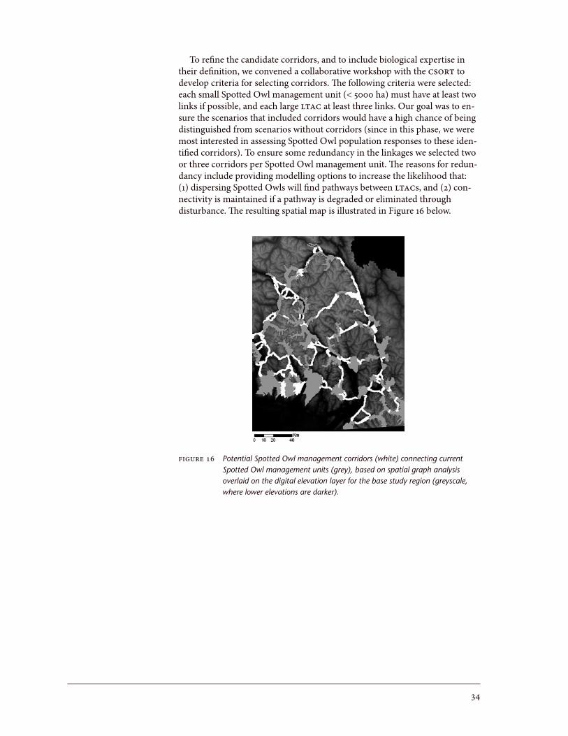
34

To refine the candidate corridors, and to include biological expertise in their definition, we convened a collaborative workshop with the CSORT to develop criteria for selecting corridors. The following criteria were selected: each small Spotted Owl management unit (< 5000 ha) must have at least two links if possible, and each large LTAC at least three links. Our goal was to en-sure the scenarios that included corridors would have a high chance of being distinguished from scenarios without corridors (since in this phase, we were most interested in assessing Spotted Owl population responses to these iden-tified corridors). To ensure some redundancy in the linkages we selected two or three corridors per Spotted Owl management unit. The reasons for redun-dancy include providing modelling options to increase the likelihood that: () dispersing Spotted Owls will find pathways between LTACs, and (2) con-nectivity is maintained if a pathway is degraded or eliminated through disturbance. The resulting spatial map is illustrated in Figure 6 below.

Figure 16 Potential Spotted Owl management corridors (white) connecting current Spotted Owl management units (grey), based on spatial graph analysis overlaid on the digital elevation layer for the base study region (greyscale, where lower elevations are darker).

35

7 POPULATION EVALUATION COMPONENT

A spatially explicit demography model was developed in the framework to: () test ecological hypotheses about possible causal factors (e.g., predators, competitors, habitat loss) of population decline and how they affect status of a species at risk (i.e., the Spotted Owl in this case study); and (2) provide esti-mates of the likelihood that the modelled population could recover to selected target population sizes, and/or persist for long time periods under alternative management scenarios. Thus, the demography model provides researchers and managers with a tool for assessing potential influences of management and environmental changes on future population status.

Use of demographic analyses and modelling to aid decision-making has a well-established history in natural resource management (Beissinger and Westphal 998). Whether more traditional tools such as life table analysis, or more recent approaches such as stochastic population viability analysis (PVA), are used, demographic models integrate multiple interactions among ecologi-cal processes and their effects on the distribution and sizes of populations (Boyce et al. 200; Dreschler et al. 2003; McCarthy et al. 2003). Yet, despite their history and acknowledged utility, building credible demographic mod-els remains a challenge. In particular, any demographic model requires a substantial dataset of population sizes and trends over time, along with measures of associated ecological data (e.g., habitat suitability, climate, topog-raphy) for adequate model parameterization, verification, and validation. The Spotted Owl case study in British Columbia lacks demographic information, therefore our demographic modelling approach was intended primarily to produce indicators of Spotted Owl population status that could be used to rank proposed management strategies relative to one another—not to predict actual Spotted Owl populations. We also developed analytical methods to overcome the limitations imposed by uncertainties in many of the model parameters.

In the sections below, we describe the concepts in the population model and their implementation into the demographic model used for analyses in the case study. Our data sources were a combination of published literature, unpublished data from ongoing research, and expert opinion (derived from workshop discussions with the research sub-group of the CSORT as described in Section .4). For the Spotted Owl case study we used the demographic model primarily to: () explore the effects of different land management poli-cies on potential trends in populations, given some assumptions about the characteristics of the population; (2) understand implications for small popu-lations; and (3) identify potential impacts of threats due to Barred Owls on Spotted Owl population recovery. These are illustrated below.

7.1 General Description of the

Individual-based Population Model

The population model is a general, spatially explicit, stage-based model that simulates the demographic fates of individual vertebrates in a semi-spatial manner. That is, the model represents individuals in specific locations (primarily in known active sites or potential breeding sites), and applies stochastic survival, reproductive, and mortality rates to each individual by location and type of interaction with other individuals (e.g., mating or competitive). The model is semi-spatial in the sense that the movements modelled are natal (movements of juveniles from natal sites to a potential

36

nest site location) and breeding dispersal movements (movements of adults between a breeding nest site to a potential new breeding nest site), while other movements on the landscape are not simulated.

7.. Life stages and population structure The population model represents three life stages with a survival rate (S) for each stage: juveniles, non-breeders (sub-adults and single non-breeding adults; SAdults), and breeding adults (Figure 7), as well as an annual recruitment rate (F). These demographic rates are assumed to be the true underlying population-level rate, and empir-ical estimates for them have been corrected for effects of local immigration or emigration (Anthony et al. 2006). The model initiates the population based on the number and location of occupied sites (nest site locations containing either SAdults or breeding adults) from an existing inventory, and uses fecun-dity estimates and an estimated proportion of SAdults (see Table 5 for definitions).

The specific rules for population initiation are as follows:

• The initial number of breeding adults will be equal to the number of active nest sites specified (depending on whether nest sites are occupied by single non-breeders or breeding pairs).

• The initial number of juveniles is determined by evaluating fecundity and clutch size for each active nest site occupied by a breeding pair.

• The initial number of single non-breeding adults is scaled to the number of breeding adults by assuming that a specified proportion of breeding adults are single non-breeding adults in a given year. This reflects the fact that not all breeding adults are mated in a given year, and also reflects the difficulty of accurately locating and censusing non-breeding adults.

• The order of priority (highest to lowest) for placement of SAdults is: () singly in active sites determined from inventory with no other SAdults (i.e., non-territorial); then (2) in suitable habitat within the study area, but excluding habitat in territories containing occupied active nest sites.

F

Ssa Sa

Sj

Juveniles Sub-adults/ Single adults

Breeding adults

Figure 17 Diagram representing life stages and transitions in the population model. F = annual recruitment rate (number of young per breeding pair); Sj = annual survival rate of juveniles; Ssa = annual survival rate of single adults and sub-adults; Sa = annual survival rate of breeding adults.

37

7..2 Population dynamics Table 6 lists the parameters used by the population model. At each time step in the model, each individual in the population is assessed for survival and probability of reproducing. The real-ized clutch size for successful breeding pairs (accounting for all sources of pre-fledgling mortality) is selected from a probability distribution. All sur-viving juveniles and SAdults can undergo dispersal. Breeding pairs may also separate and disperse, in which case they are demoted to single adults.

Table 5 Description and rules for each Spotted Owl life stage as defined in the population model

Life stage Description Assumptions

Juveniles Newly fledged offspring 1. Juveniles (defined here as young that have survived all (age < 1 year) sources of pre-fledgling mortality) potentially disperse before they reach age 1. If they survive, they transition to single non-breeding adults at the beginning of the subsequent year (the start of the breeding season). Not all juveniles disperse. 2. Mortality rates are influenced by quality of the natal territory.

Single Sub-adults, single 1. Can be non-territorial (up to one SAdult can occupy an activenon-breeding non-breeding adults site territory containing an existing breeding pair).birds (SAdult) (age ≥ 1 year) 2. Can occupy and move through habitat outside of active site territories. 3. SAdults move randomly within a region defined on the cost surface up to a specified maximum dispersal distance. 4. SAdults can form a breeding pair and establish an active nest site and a territory containing and active nest site, if: (a) a conspecific of the opposite sex is present, (b) one or more potential nest site locations are available, and (c) if specified, other existing active nest sites (i.e., social cues for facilitating breeding) are within the least-cost movement region. 5. SAdults do not reproduce.

Breeding adults Breeding adults in a 1. Breeding pairs occupy an active nest site and establish and(Adult) breeding pair defend a territory around that active nest site. (age ≥ 2 years) 2. Once an active nest site has been established, the breeding pair does not move. 3. Female breeding adults reproduce if the value drawn from a normal distribution exceeds the specified minimum value for reproducing. Clutch size and number of fledged young are determined as in Table 6. 4. If one of the pair dies, then the other transitions to an SAdult, it leaves the active site, and the territory containing the active nest site becomes deactivated. 5. Each year, if a randomly drawn value from a normal distribution exceeds the parameter specified for separation (Table 6) then both individuals transition to SAdults and the active site is deactivated. 6. A deactivated area immediately becomes available for recruitment as a new potential nest site. While previous occupants of the site (either as SAdults or members of a newly formed pair) can return to this site, this is not guaranteed.

38

Breeding pairs occupy and defend a territory surrounding the active site. Active site territories are created using a similar algorithm to the territory packing model presented in Section 5.

Dispersal is simulated once per year by randomly selecting a location within a defined region of potential movement locations. Locations of suit-able habitat are identified using a movement cost surface (see Section 4) within a region that encompasses the specified maximum movement distance measured as Euclidean distance. Single adults and sub-adults can only be within an existing breeding pair territory if there are no other juveniles, sin-gle adults, or sub-adults present.

Nest site recruitment can occur when a dispersing SAdult encounters an-other SAdult of the opposite sex within the potential movement region. The probability of pair formation is selected from a normal distribution with mean and standard deviation specified in Table 6. If a nest site is chosen to be occupied, its location is selected from the potential nest site location layer (i.e., the cell with highest proportion of nest habitat within an 00-m buffer surrounding it). Newly occupied nest sites cannot be located closer than a minimum distance from existing nest sites (Table 6) representing spacing be-haviour. Their formation can also be restricted to occur only when existing nest sites coincide with both the movement region of the dispersing individ-ual and the presence of a potential mate. If invoked, this rule adds a “social cue” component to the likelihood of forming a breeding pair, such that the presence of other nearby breeding pairs increases the likelihood that unmat-ed individuals of opposite sex will themselves form a breeding pair (assuming suitable nest sites are present).

Note that this version of the population model does not include spatially localized adjustments on mortality at the occupied nest site as a consequence of anthropogenic habitat fragmentation and edges (e.g., increases in potential nest predators such as corvids or mammals). These effects have been suggest-ed as a possible effect in Spotted Owl demography studies in the United States (see Courtney et al. 2004 for reviews of the evidence), as well as in other forest-dependent species (e.g., Marbled Murrelets in British Columbia; Canadian Marbled Murrelet Recovery Team 2003), but similar relationships are too poorly known for Spotted Owls in British Columbia to develop plau-sible relationships.

The model also includes the facility to implement a net immigration rate. Immigrants are initiated at locations that can be specified in a number of ways, such as locations along the borders of the study area, at specified “re-lease” points within the study area, or at randomly generated locations in suitable habitat.

Several studies demonstrate that the amount and distribution of habitat at each time step directly influences population vital rates by: () determining the location of potential nest sites within the range; (2) determining the sur-vivorship of owls in existing territories containing active nest sites, based on the proportion of suitable habitat within the territory; (3) influencing repro-ductive success at nest sites (Bart 995; Franklin et al. 2000; Olson et al. 2004; Dugger et al. 2005); and (4) determining the spatial extent of potential move-ment locations for dispersing juveniles and single/sub-adults. In most of these studies (except Franklin et al. 2000), the strongest relationship appears to be a dependency between habitat quality and the survival of adults in breeding pairs.

39

This spatial dependency linking population vital rates and territory quality was implemented in the model by assuming that adult survivorship varies with the proportion of suitable habitats in the territory containing the nest site (e.g., Bart 995). Adult survival for members of a breeding pair was there-fore computed for each subregion as a function of the proportion of suitable habitat within the territory (Figure 8). This is a simple form of the “habitat fitness” concept introduced by Franklin et al. (2000) and Olson et al. (2004), although we did not have sufficient demographic data to derive as detailed a function as those researchers did. We developed our function as follows, using survival rates as shown in Table 6 and measurements of territory quali-ty for the recent historical population (RHP) in British Columbia. For a given ecological subregion, we assumed that the range of survivorship rates is one standard deviation around the mean annual survival rate corresponding to the subregion giving the maximum and minimum values for the Y-axis (see Table 6). Similarly, the range in territory quality was determined from the minimum and maximum proportions of habitat within territories identified for locations known to be actively used by the recent historical population (N = 47 confirmed occupied locations between 997 and 2005; I. Blackburn and J. Hobbs, B.C. Ministry of Environment, pers. obs., Nov. 2005), giving points on the X-axis from which to interpolate survival. We assumed that minimum observed survivorship of breeding owls would occur at the mini-mum observed habitat quality, and the converse for maximum survivorship and habitat quality. Breeding adult survival for any projected territory was therefore determined by interpolating between the minimum and maximum survivorship expected for the ecological subregion based on the measured proportion of habitat in the projected territory containing a breeding pair. Because owls appear to be able to use areas outside the breeding territory at certain times of the year, there is a minimum threshold for the effect of habi-tat quality in the breeding territory on adult survivorship, even if the habitat quality of the territory declines to zero. The lack of Spotted Owl field data ne-cessitated estimating the threshold for this case study based on a consensus of expert opinion within the CSORT (achieved through workshop discussions as described in Section .4).

1.0

0.9

0.8

0.7

0.6

0.5

0.4

0.3

0.2

0.1

0.0

Bree

ding

adu

lt su

rviv

orsh

ip

0.0 0.1 0.2 0.3 0.4 0.5 0.6 0.7 0.8 0.9 1.0

Proportion of suitable habitat in territory

Figure 18 Interpolated linear function for estimating breeding adult survival. Survival is interpolated based on the percentage of suitable habitat within the territory surrounding the active site location (see text for details) for the continental subregion.

40

Table 6 Parameters specifying vital rates and behaviour for the British Columbia Spotted Owl population (mean ± SD) taken directly or calculated from the listed sources. Where no estimate of variation is reported, we assume SD = 10% of the mean. Data from specific areas in Washington (names in square brackets), used as surrogates for the ecological subregions defined in this model, are described by Anthony et al. (2006)a.

Maritime Submaritime Continental Vital rate/Parameter [Olympics] [Rainier] [Cle Elum] Source and Comments

Probability that a breeding 0.293 ± 0.228 0.253 ± 0.202 0.574 ± 0.258 Table 5 in Anthony et al. (2006)pair will fledge young Nowls = 883 Nowls = 184 Nowls = 423 Nyears of data = 16 Nyears of data = 11 Nyears of data = 14

Survival of adults in 0.855 ± 0.219 0.856 ± 0.295 0.860 ± 0.295 Tables 1, 13 in Anthony et al. (2006)breeding pairs Nowls = 395 Nowls = 217 Nowls = 423

Single/non-breeding 0.72 ± 0.55 0.83 ± 0.06 0.86 ± 0.0.09 Tables 1, 13 in Anthony et al. (2006) calculated by combiningadult survival Nowls = 74 Nowls = 15 Nowls = 55 ages 1 and 2

Juvenile survival 0.575 ± 0.058 0.305 ± 0.031 0.157 ± 0.016 Note that Anthony et al. (2006) do not present estimates of juvenile survival. The estimates here were obtained from solving a stage model using the other vital rate estimates in this table

Probability of producing p(1 egg) = 0.42 p(1 egg) = 0.42 p(1 egg) = 0.42 Gutiérrez et al. (1995) cited by Chutter et al. (2004)b

1, 2, or 3 eggsa p(2 eggs) = 0.56 p(2 eggs) = 0.56 p(2 eggs) = 0.56 p(3 eggs) = 0.02 p(3 eggs) = 0.02 p(3 eggs) = 0.02

Number of years before 1 1 1 Assuming that newly formed breeding pairs cannot reproduce untilpair will reproduce the following year

Probability that a breeding 0.066 0.066 0.066 Forsman et al. (2002)pair will separate and undergo breeding dispersal

Proportion of breeding 0.066 0.066 0.066 Forsman et al. (2002) pairs as single non-breeding Some birds in a split breeding pair will retain the site and find newadults mates quickly, so the proportion of territorial birds that become singles may be less than the proportion of birds that leave a site. (J. Buchanan, Wash. Dept. Fish Wildl., Olympia, Wash., pers. obs., Feb. 2004.)

Maximum natal dispersal 60 km 60 km 60 km Forsman et al. (2002)distance Median of maximum values reported for males and females

4

Table 6 (Continued)

Maritime Submaritime Continental Vital rate/Parameter [Olympics] [Rainier] [Cle Elum] Source and Comments

Probability of breeding 0.78 0.78 0.78 LaHaye et al. (2001)pair formation, given In a southern California population, 78% settled in previouslyproximity to each other, occupied territories, and 16% settled in territories adjacent toavailable nest habitat and occupied sitesconspecifics

Minimum distance 1 km 1 km 1 km J. Buchanan, Wash. Dept. Fish Wildl., unpublished databetween nest sites

Annual immigration ratec 1% 1% 1% Expert opinion (J. Buchanan, Wash. Dept. Fish Wildl., pers. obs., Dec. 2004)

Annual emigration ratec 1% 1% 1% Expert opinion (J. Buchanan, Wash. Dept. Fish Wildl., pers. obs., Dec. 2004)

a Fecundity rate indicated here as number of female young produced per adult female (see Anthony et al. 2006).b Chutter, M.J., I. Blackburn, D. Bonin, J. Buchanan, B. Costanzo, D. Cunnington, A. Harestad, T. Hayes, D. Heppner, L. Kiss, J. Surgenor, W. Wall, L. Waterhouse, and L. Williams. 2004. Op. cit.c This variable can be set as a parameter, but it was not used for the case study.

42

7.2 Application of the Population Model

in the Case Study

For these analyses, the spatially explicit population model component of the Spotted Owl model framework was initialized with one or more estimates of the current Spotted Owl population. Together with a chosen set of vital rates and other population parameters, we projected population dynamics up to 50 years into the future,33 depending on: () the spatial time series of habitat maps generated by the landscape dynamics models, and (2) the locations of potential territories that could be occupied by dispersing Spotted Owls. To maximize model processing efficiency, an upper limit on population size was imposed to terminate the model when the population reached 250 individu-als. This upper limit was chosen in consultation with the CSORT. Modelled populations of that size with stabilized vital rates are unlikely to decline to extirpation within the model time frames. Details on parameter values used are provided below.

7.2. Calibration of population vital rates There are no empirical estimates of vital rates for British Columbia’s Spotted Owls, and appropriate extrapola-tions of estimated rates from U.S. studies are uncertain. A comprehensive projection of all likely population vital rates, as has been undertaken for other species in British Columbia (e.g., Steventon et al. 2003 for Brachyram-phus marmoratus), was not practical given the time constraints of this study. We therefore developed a “calibrated” set of stable-state population vital rates to use as a benchmark for testing management scenarios and biological hy-potheses, from which the resulting projections could be compared. We first calibrated the population’s vital rates to allow the population to remain at an approximately stable population size under long-term equilibrium (LTE)34 natural conditions (Table 7). We ran all feasible combinations of vital rates (Table 6) and selected sets for each ecological subregion, which provided the most reasonable interpretation of plausible population dynamics for the Spotted Owl under this stable-state assumption.

By using the calibrated rates to produce projected population responses under imposed landscape disturbance (e.g., roads, resource extraction), we can partition out independent effects of habitat manipulations on relative trends in population results, while eliminating confounding effects from other natural disturbances or other unknown demographic factors. For this reason, we used the set of calibrated stable-state vital rates instead of extrapo-lated, current U.S. field estimates for most of the analyses discussed elsewhere

Table 7 Selected calibrated vital rates for a stable-state population of Spotted Owls on a long-term equilibrium (LTE) landscape

Ecological subregion Fecundity Juvenile survival Adult survival

Maritime 0.352 0.563 0.906Submaritime 0.304 0.563 0.882Continental 0.689 0.563 0.912

33 For population questions we focused primarily on relatively short-term habitat change and restoration (0–50 years) because options for habitat restoration are most constraining in the shorter term, and because uncertainties increase with increasing time horizon.

34 We projected an LTE landscape using a natural disturbance model to estimate quasi-stable-state natural conditions. We used the disturbance regimes from Table A2. (Appendix 2), and projected the model forward for 0 000 years.

43

in this document. Specifically, this approach enabled us to address the follow-ing limitations:

. Current field estimates of vital rates confound all biological and manage-ment effects on population dynamics, as well as short- (0–20 years) and long-term (> 20 years) variability in trends. Although our model structure allows some partitioning of these effects in principle, confounding in the empirical input parameters reduces the chance that potential changes to population trends due to changing management policy may be reflected in the model outcomes. This calibration enhances our ability to tease apart and rank-order the implications of management policy.

2. The present empirical rates project a strongly declining population. Be-cause of the time scale of the landscape’s response to management, the population projected using present rates is likely too low to be able to re-spond, at least in the short term, to any changes in habitat configuration or amount, and some useful policy options for future Spotted Owl habitat management may not be detected.

3. Additional relationships such as dispersal and recruitment may modify the model responses, given the small population size and population rates obtained from empirical analysis of demographic data. It would not be ap-propriate to project the population using current vital rates as there are additional complexities in this model that are assumed to be included in the empirical estimates of fecundity and survival.

We note that because some non-independent interactions between habitat quality and vital rates also occur and are included in the model, our method precludes being able to make unambiguous statements about the effects of habitat manipulations on population trends. There are insufficient empirical data about the strength of those interactions in British Columbia to be able to draw absolute conclusions.

Any choice of vital rates necessarily imposes some assumptions and limi-tations on the model. In particular, vital rates prescribe a set of life-history assumptions about the population. For a given set of vital rates, life stages may respond slightly differently to certain management options than to oth-ers. If true vital rates are not known with certainty (as is the case with Spotted Owls in British Columbia), then potential population responses to manage-ment cannot be projected with certainty either. Note that while we have used ecological subregion-specific vital rates, population results are not reported by ecological subregion for two reasons: () individual movements are not re-stricted to subregion boundaries, and (2) conservation options are primarily (although not completely) formed at the population, and not subpopulation or ecological subregion, level.

7.2.2 Indicators of population status and trends Our primary indicator of population status is the mean trend in population size relative to a base-case scenario in the short term (0–20 years) and the longer term (20–50 years). We do not use probability of population persistence, risk of extinction, or similar measures often used in population viability analyses (PVAs) because:

. high uncertainty in both the current inventory of the population, the true population vital rates, and additional interactions affecting the dynamics of the population make such a probability measure difficult to interpret;

44

2. several studies suggest that estimates of time to extinction or extinction probabilities in PVAs are often inaccurate, even when using less explicit approaches such as “diffusion approximations” (Fieberg and Ellner 2000; Wilcox and Possingham 2002);

3. reliability of PVAs is dependent on the time-series of empirical population data (Ludwig 999), and we did not have a sufficiently long time series; and

4. a more reliable estimate of population persistence would require a very large number of simulations.

This is consistent with the conclusions of Reed et al. (2002), who recom-mend that PVA not be used to determine minimum population size or to give a specific probability of extinction. Despite uncertainty and lack of empirical data, PVA remains useful for comparing alternative management policies and the relative risks of species extinction (Brook et al. 2002).

7.3 Exploring Interactions between

Land Management Policies and

Population Size

Some key questions are highlighted by our current knowledge of (and uncer-tainties about) present population size, trend and habitat management issues, and analyses using the model framework. These questions include:

. how important could small population effects be in influencing potential chances for recovery;

2. how might alternative land management policies interact with different population sizes as a factor in influencing future recovery potential; and

3. if amount of habitat is presently limited, could recovery of habitat over time influence the potential for recovery for a given population size and land management assumptions?

These issues are likely confounded for a given set of assumptions about initial population size, land management rules, and time frame. We illustrate the potential of the framework to partition effects of some of these issues using the simulation experiments described below.

We asked three questions:

. how important is initial population size in determining short-term popu-lation trends, given a defined land management scenario;

2. how important is a land management scenario in determining short-term trends in modelled populations, given an initial population size; and

3. how important is initial state of the landscape in influencing short-term trends in modelled populations, given an initial population size and land management scenario?

We designed a factorial set of 8 simulations to partition these effects using the starting conditions outlined in Table 8. We projected forward to a maxi-mum of 50 years (as discussed in Section 7.2). We ran 0 iterations for each simulation experiment. All simulations were conducted using the following assumptions:

. Modelled populations use the calibrated vital rates (described above).2. Initial active nest sites were selected at random from the potential territo-

ries available at each time period. 3. There is no net immigration or emigration.

45

With these simulations, we found the following general effects (Figure 9):

Population size (using stable-state vital rates):

• There is considerable uncertainty over all conditions in the projected pop-ulation size, even for projections of 25 years or less, indicated by the width of the error bars. Caution is needed in interpreting error bars in this con-text—the state of a particular projected population in year t+ is strongly autocorrelated to its state in year t. Therefore, within-projection variation cannot be independent, although among-projection variation is.

• Smaller initial populations (25 breeding sites) are much less likely to have a stable or increasing short-term trend than larger initial populations (50 breeding sites), all other factors being equal. In particular, very few of the projected population runs with small starting populations (~59–68 indi-viduals) resulted in increasing trends over a short period (25 years from the start of the simulation). Although this observation indicates a small probability of recovery for a small population (assuming vital rates can be stabilized), our model data are not sufficient to assign persistence proba-bilities that can be interpreted for the current population based on these projections.

• Over all conditions, no modelled population is 00% guaranteed stable or increasing by years 2–25, although there is an increasing chance that pop-ulations will stabilize or increase by that time period, no matter what the initial size or land management scenario.

• Examining individual runs for each factor combination, it appears that if modelled populations increase to over 70 individuals, their chances of re-maining stable or increasing become greater than 50% irrespective of other conditions.

Land management scenario:

• Over the three scenarios we tested, there is no clear and consistent evi-dence that alternative management policies within this range affect the probability that populations will become stable or increase within the very short term (0–0 years).

Table 8 Alternative sets of assumptions for the factorial simulation experiments partitioning effects of main factors affecting short-term modelled population trends

Initial population size Land management scenarioa Time period

• 25 breeding sites • AgingOnly—no disturbances • initiate at year 0 (65–71 individuals) • InterimSOM—interim habitat protection • initiate at year 20• 50 breeding sites recommendations of the CSORT, protecting • initiate at year 40 (133–141 individuals) existing and proposed Long Term Activity Centres, and protecting some connectivity corridors for dispersal • NoSOM—current Spotted Owl management designations and associated management regimes for Spotted Owl are not applied

a For scenario details see Section 0.

46

300

250

200

150

100

50

0

Tota

l pop

ulat

ion

size

0 5 10 15 20 25 30 35 40 45 50

Year

300

250

200

150

100

50

0

Tota

l pop

ulat

ion

size

0 5 10 15 20 25 30 35 40 45 50

Year

300

250

200

150

100

50

0

Tota

l pop

ulat

ion

size

0 5 10 15 20 25 30 35 40 45 50

Year

Figure 19 Potential effects of initial model population size, land management scenario, and starting year (landscape state) on short-term trends in modelled populations (mean ± SD). See Table 7 for details. Simulations starting at year 0 (top); year 20 (middle), and year 40 (bottom).

AgingOnly 25 breeding sitesInterimSOM 25 breeding sitesNoSOM 25 breeding sitesAgingOnly 50 breeding sitesInterimSOM 50 breeding sitesNoSOM 50 breeding sites

47

• There are only weak indications that increasing levels of habitat protection as defined in this range of scenarios increases the probability of popula-tions becoming stable or increasing beyond 25 years (to 50 years). Because we did not run population simulations beyond 50 years, we did not inves-tigate the likelihood that actions taken in the short term might lead to long-term (> 50 years) adverse or beneficial effects on population trends.

Starting point (habitat change):

• There is weak evidence to suggest that habitat recovery (i.e., recruitment of new habitat) over short periods can improve the probability that popu-lations will become stable or increase within 2–25 years of initiation. As noted, this is not surprising, as the amount of restorable habitat available in the next 20 years is relatively small. This effect is dependent on popula-tion size—the larger the initial population, the more likely this effect will be.

Clearly, the stochastic variation in population projections dominates re-sults, and tends to obscure underlying trends. This does not mean that the effects do not occur, but simply means that interpretations must be made in the context of considerable uncertainty in the resulting projected population trends. Because we used random potential nest site locations to initiate our starting populations, these results may underestimate trends that could occur if locations were selected on the basis of habitat quality (e.g., under an aug-mentation scenario). We caution that extrapolation of these findings to infer long-term trends for true population sizes is not yet justified on the basis of the assumptions used in the models.

7.4 Exploring Potential Barred

Owl Effects with the Population Model

The Barred Owl (bdow) has been identified as a significant potential threat to Spotted Owls in many areas of their range, including British Columbia (Gutiérrez et al. 2006). There is a general lack of understanding of Barred Owl ecology and demography within the range of the Spotted Owl in both British Columbia and the United States, although studies are under way. Interactions between the two species are characterized as competitive, favouring Barred Owls (Courtney et al. 2004). Recent evidence from Wash-ington State indicates that where habitat use by Barred Owls and Spotted Owls overlaps, Barred Owls may compete with Spotted Owls for resources. For example, where Barred Owls occur within 0.8 km of a Spotted Owl nest site there is a greater likelihood that the Spotted Owl site will not be occupied compared to Spotted Owl sites with more distant Barred Owls (Kelly et al. 2003). Both species are of similar size and have been reported on occasion to interbreed (Hamer et al. 994). One study from Washington State suggests some spatial separation may occur between Barred Owls and Spotted Owls because Barred Owls tend to occupy lower-elevation areas closer to rivers, while Spotted Owls also occur upslope at higher elevations (Pearson and Livezey 2003). In other areas, however, spatial overlap between the two owl species appears extensive (Courtney et al. 2004). Understanding the influ-ence of Barred Owl on Spotted Owl is important, as such interactions may compromise the effectiveness of land management strategies designed for Spotted Owl recovery.

48

The model framework provides several ways to examine possible conse-quences on the Spotted Owl population from different possible competitive interactions between the species. Potential mechanisms of interaction in-clude: () breeding pair separation in Spotted Owls by displacement of one member by Barred Owl; (2) reduced survival and/or fecundity in adult Spot-ted Owls by exclusion from resources by Barred Owls; (3) reduced estimated amounts of functional habitat available to Spotted Owls; and (4) reduced dis-persal efficiency by Spotted Owl juveniles. These types of interactions in the framework are modelled respectively to: () alter the parameter specifying probabilities of pair separation (Table 6); (2) alter survival and fecundity vital rates for adults and survival for SAdults; (3) reduce the estimated functional habitat area available to Spotted Owls (e.g., reducing territory size) in areas of Barred Owl occurrence; and (4) modify the movement least-cost surface for dispersal in areas containing Barred Owls. These model tests can be conduct-ed with varying degrees of spatial explicitness. Without Barred Owl invento-ry maps, potential effects on Spotted Owl population dynamics were best explored using simple proportional changes in parameter values. However, if an inventory map of Barred Owl occurrence does exist, then expected chang-es in the above parameters can be spatially modelled as occurring only where Spotted Owls and Barred Owls are known to overlap.

As a preliminary experiment to illustrate how to explore one or more of these interactions between Spotted Owls and Barred Owls and to gain under-standing of their potential impacts on Spotted Owl population dynamics, we tested incremental increases in Spotted Owl breeding pair displacement by Barred Owl using a population with calibrated population vital rates and 50 randomly selected potential Spotted Owl nest site locations (i.e., not depen-dent on current inventory). We projected this modelled population forward for 30 years under land management assumptions of no disturbance (AgingOnly), representing a control scenario (no habitat or landscape modification) against which to compare other scenarios. Since there was no inventory map of Barred Owl sites, we incrementally increased the probabili-ty of breeding pair separation (default rate = 0.066 per pair per year; Table 6) for all breeding pairs by percentage of the default value to assess how pair displacement by increasing numbers of Barred Owls could reduce chances of population recovery in Spotted Owls (or increase probability of population decline). We conducted 0 iterations of the model for each parameter change.

The preliminary results suggest that breeding pair displacement by Barred Owl can have a significant effect on modelled Spotted Owl populations (Figure 20), and that negative effects increase with increasing probability of pair separation. Increasing the annual probability of pair separation by 300% or more has a large effect on population trend, while negative effects with lower separation probabilities than that level are relatively small.

We caution that this analysis is preliminary only. More precise estimates of the extent of this potential effect requires a spatial probability map of the likelihood of Barred Owl occurrence in Spotted Owl ranges based on avail-able Barred Owl inventory data, and spatial models of the suite of interaction mechanisms (e.g., displacement and competition) between the two species. Such analyses are presently beyond the scope of this work, but the analyses above do demonstrate the ability of the framework to test hypotheses such as these.

49

8 EVALUATING CURRENT AND FUTURE HABITAT QUALITY USING A BAYESIAN BELIEF NETWORK (BBN)

A primary issue in land use planning is identifying critical habitats required to ensure survival of known populations of threatened species, and those required to achieve recovery goals for such populations or species. We ex-tended the framework to address this type of issue by developing a method of integrating estimates of the relative value of each hectare of habitat to meet the habitat requirements of the species at three spatial scales relevant to criti-cal life history requirements of many species: site (stand scale or below), territory, and population (landscape). This model component also develops these estimates at different points in time (current and future) such that habi-tat of sufficient quality can be identified to meet present and future targets (also see Section 9). We used a BBN to develop this cross-scale habitat evalua-tion tool.

Methods of defining and designating critical habitat for recovery plans are actively being developed by Federal agencies (Environment Canada 2004). Prescriptive methods for critical habitat delineation depend on such factors as the completeness of the inventory, the approach taken to develop the re-covery plan for the species (e.g., expert judgement, quantitative analysis, simulation modelling), and the specific recovery goals. Because a modelling approach that integrates ecological processes at these three spatial scales (site, territory, and population) has been used to assist in recovery planning for the Spotted Owl population in British Columbia using the framework described in this document, the essential elements required to evaluate critical habitat at these scales (Government of Canada 2002) can be assessed by the BBN model. These elements include quantitative estimates of the necessary and

160

140

120

100

80

60

40

20

0

Tota

l pop

ulat

ion

size

0 3 6 9 12 15 18 21 24 27 30

Year

100%200%300%400%500%600%

Figure 20 Potential effect of displacement of Spotted Owl breeding pairs by Barred Owl projected population sizes. The graph depicts mean (±1SD) for two scenarios) projected population sizes of Spotted Owls over 10 runs with increasing probabilities of breeding pair separation, expressed as percentages of the default parameter value (set at 100%) over 30 years with a starting population of 50 pairs and sAdults.

50

sufficient areas (hectares) and qualities (composition and configuration) of proposed critical habitat required to support the population now and in the future. We describe our approach to evaluating the quality of habitat from the perspective of critical habitat delineation below.

The BBN model as developed for this case study is relevant to species that () form territories (territory attributes), (2) exhibit a form of spatial density-dependence (i.e., proximity to nearest sites and nearest territories, where density of known and prospective sites is a determinant of demographic pro-cesses), and (3) are of sufficient body size and vagility so as to respond to three spatial scales (site, territory, population). Different BBNs could be con-structed for species that do not exhibit these characteristics, or that exhibit only some of them. Alternatively, this BBN could be modified and reparame-terized to reflect the spatial scale requirements of other species.

8.1 General Description of the

Habitat-quality BBN

We used a BBN as the analytical tool to estimate integrated habitat quality, linking the time scales and spatial requirements for helping inform the selec-tion of critical habitats. BBNs are represented by a diagram of boxes (termed nodes, representing variables) and arrows (termed links, representing func-tional relationships among variables). Each node can assume one or more user-defined categorical or numeric states, and has a conditional probability table that expresses the likelihood of each state, conditional on the likelihood of each state for the nodes feeding into it (the parent nodes). The conditional probability tables can be populated directly from files of observed data cases, entered manually, or derived mathematically. Belief weightings can be assigned to input parameter values (nodes with no parents), and to relation-ships among parameters (e.g., linear or non-linear relationships of habitat quality to nesting density). Results are provided as a range of possible out-comes, each with a probability (plausibility weighting) resulting from the interaction of variables through the network. Several studies (Reckhow 999; Marcot et al. 200; Riemen et al. 200) provide further background and ex-amples using BBNs in natural resource management situations.

The purpose of developing a BBN in the framework is to enable users to refine rules for assessing habitat quality for a given study species—rules that are often difficult to parameterize. For example, differing objectives for habitat protection may change the importance weighting for a cell’s habitat quality classification. The BBN is intended to: () capture uncertainty of the habitat relationships that define habitat quality for a species, and (2) evaluate relative weightings for different structural and spatial habitat attributes at each location as they relate to different ecological requirements of the study species. Together, these attributes may determine the value of each spatial habitat unit in forming critical habitat. As applied in this case study, the BBN builds upon cross-scale habitat and population concepts for owls first devel-oped by Carey et al. (992), King et al. (997), and McComb et al. (2002), while also offering a flexible tool for critical habitat selection.

The conceptual structure of the BBN as defined in the framework is shown in Figure 2 depicting the three spatial scales or contexts. Specifically, the habitat quality of each habitat cell is evaluated by () creating rules for deter-mining the relative value of the habitat attributes defined for the cell in each particular context (site, territory, population), and (2) defining rules for de-termining the influence of the proximity of that cell to other habitat features expected to be relevant at each scale on the cell’s habitat value. By using rules for weighting the relative influence of attributes and proximity to other fea-

5

Habitat ranking criteria factors

Proximity to nearest territories

Density of known sites

(buffer)

Density of prospective sites

(buffer)

Population habitat quality

(relative)

Territory habitat quality

(relative)

Integrated habitat quality

(relative)

Territory attributes

Site habitat quality

(relative)

Proximity to nearest sites

Site atttributes

Figure 21 A conceptual structure of the BBN developed for ranking habitat quality for each cell using outputs from other components of the framework and weighting rules specified within the BBN. Colours shown identify nodes specific to each scale context – green = site-scale; orange = territory-scale; light blue = population scale.

tures at each scale, an expected habitat quality evaluation is made for that cell in each of the scale contexts. Note that these evaluations are done indepen-dently at each scale, and the results at each scale can be reviewed separately. Note also that these evaluations are intended to be relative evaluations and not absolute scores of habitat quality. Finally, the habitat quality rankings from each scale are combined together into the final integrated habitat quali-ty ranking that is applied to each cell (the bottom node of the BBN in Figure 2).

Outputs from the BBN are classifications of each habitat cell in terms of its relative quality in each spatial context (site, territory, and population). Cells are ranked at each time period. The results are used to rank the importance of each location’s ability to fulfill critical habitat requirements. Output maps illustrate the relative rankings of each cell at each scale. We used the Netica™ BBN software (Norsys Software Corp., Vancouver, B.C.35) to build the proto-type.

8.2 Alternative Definitions of

Centroids in the BBN

An important concept in the conceptual structure of the BBN is spatial prox-imity of a given location to the nearest active nest sites or potential sites that may be occupied now or in the future (Figure 2). Not surprisingly, there is considerable uncertainty about how the future recovered population may be distributed within its former range in British Columbia, and hence where po-tential dispersing owls are likely to come from in the future. Because our BBN uses spatial proximity to both current and potential future locations of nest-ing habitat as a factor in assessing potential critical habitat, we needed to estimate where such locations may be in the future. Our method for doing this estimation uses the connectivity analysis approach described in Section 6. We assume that the future population is most likely to be in areas of rela-tively well-connected nesting habitat. However, there are other factors than just nesting habitat to consider, and currently there is no consensus on their relative importance. Because the results of the BBN are intended to be used towards identification of critical habitat, we wished to investigate the effect of using different, yet plausible, rules for determining these future locations on the habitat quality assessment results of the BBN.

35 Mention of trade names is for information only and does not indicate an endorsement.

52

Accordingly, as a preliminary step before running the BBN, we identified nesting habitat centroids using the connectivity analysis component (Section 6) together with the base habitat classifications (Section 4). The results were then used as one of the inputs into the BBN. The following rules were speci-fied in applying the connectivity analysis, based on two workshop discussions with Spotted Owl biologists (see Section .4).

. Specify a target number of home ranges. In all cases, we used a target of 25 over the species’ range, consistent with the goals of recovery planning (see also Section 9).

2. Specify potential home range size targets on an ecological subregion basis. These were generally set at 50% of the minimum required size for each ecological subregion (maritime: 907.5 ha; submaritime: 736 ha; continen-tal: 446 ha). We used 50% because the spatial graph assessment was based only on nesting habitat, and does not guarantee that high densities of nest-ing habitat are located in areas that can support feasible territories. Study of the territory model’s behaviour indicates that the highest-quality terri-tories have sizes that are less than 50% of the maximum size. Thus a 50% target combines density of nesting habitat with feasibility of establishing a high-quality territory as a criterion for defining centroids.

Other size targets were also used in some scenarios to achieve certain ob-jectives (e.g., to obtain more clusters in the continental subregion). This step was thus used to identify the best connected set of clusters that could individually support at least 0 potential home ranges, and collectively at least 25.

3. Specify a desired future nesting habitat distribution scenario. In this appli-cation, we considered two:i. Base with representation In this scenario, we allowed the connectivity

algorithm to identify the best nesting habitat clusters using rules –3 (the “base” set of rules for centroid definition), while also ensuring that at least one cluster is located in each ecological subregion. Without ap-plying this additional representation rule, all clusters will be located in the submaritime subregion, which has the highest density of potential nesting habitat in the British Columbia range.

ii. Expert opinion Nesting habitat is only one factor defining how future populations could be distributed. Accordingly, we sought opinions from the CSORT through a workshop discussion as to where the best nesting habitat clusters might be. These were then georeferenced as centroids, and used as input to the BBN as an alternate centroid scenario.

We present the BBN output using the no disturbance land management scenario over the whole Spotted Owl range, together with these two alternate centroid scenarios to investigate the effects of these alternatives on resulting patterns of habitat quality.

8.3 Application of the Habitat-quality

BBN to Identify High- quality Habitats for Recovery Planning

8.3. Specifying the habitat-quality BBN In the case study, we fully popu-lated the BBN using nodes, rules, and weights that were refined through two workshops with the research sub-group of the CSORT (Figure 22; Table 9). Building on the conceptual model (Figure 2), we proceeded systematically through the attributes and proximity variables defined for each scale to de-fine the structure as follows:

53

Use known site data?

Forest location Subregion

SPOW mgmt zone

Management unit

Land ownership code

Year from present

SPOW Habitat Quality BBNVersion 1.3

SPOW Modelling Team/CSORT2006

Site-level attributes of cellStand age (yr) until suitable habitat

Status of habitat at year

Cost distance (site) tonearest current active site

Cost distance (site) to nearest centroid

Cost distance (terr) to nearest centroid

Cost distance (terr) to next nearest centroid

N times within a Poten Terr

Territory-level attributes of cell

Avg ratio of nesting foraging

Mean propor’n in suitable habitat

Cost distance (site) to next nearest current active site

Cost distance (site) to next nearest centroid

Nearness (site) to current active sites

Nearness (terr) to current active sites

Nearness (site) to potential future breeding sites

Nearness (terr) to potential breeding sites

Default weights on known vs potential futures sites (site)

Default weights on known vs potential futures sites (terr)

Relative weight on known active sites (site)

Relative weight on known active sites (terr)

Cost distance (terr) to nearest current active site

Cost distance (terr) to next nearest current active site

Pop’n-level attributes of cell

#AS: 0–5 km radius

#AS: 5–10 km radius

#AS: 10–15 km radius

#AS: 15–20 km radius

#AS: 20–25 km radius

#AS: >25 km radius

#PTs: 0–5 km radius

#PTs: 5–10 km radius

#PTs: 10–15 km radius

#PTs: 15–20 km radius

#PTs: 20–25 km radius

#PTs: >25 km radius

Default weights on known vs potential future sites (pop’n)

Relative weight on known active sites (pop’n)

Proximity (terr) to current & potential…0–5 32.05–4000 34.44000–8000 4.968000–12000 2.5412000–9.05e6 26.1

1180000 ± 2400000

Biological habitat quality (site)vlow 4.64low 25.3moderate 21.8high 48.2

3.14 ± 0.95

Habitat quality

3.04 ± 0.97

Proximity (site) to current & potential pop’n…

3450000 ± 3300000

0–5 12.05–4000 10.54000–8000 4.998000–12000 3.5312000–1e7 69.0

vlow 4.64low 31.1moderate 19.7high 44.6

Biological habitat quality (pop’n)

2.29 ± 1.1

vlow 27.9low 32.5moderate 22.1high 17.5

Potential value for breeding SPOWvlow 46.9low 17.2moderate 21.9high 14.0

Rel. density of potential breeding site…below average 55.8above average 44.2

Rel. density of currently known sites within…below average 100above average 0 +

vlow 46.9low 33.6moderate 10.7high 8.74

Territory quality for breeding SPOW

Integrated biological habitat qualityvlow 34.3low 25.3moderate 19.6high 20.8

2.27 ± 1.1

Biological habitat quality (terr)vlow 56.2low 17.6moderate 17.0high 9.13

1.79 ± 1

Figure 22 The full habitat quality BBN as implemented in the framework for the Spotted Owl case study. All nodes are shown here with their scale-contexts identified using the colour scheme presented in Figure 21. Nodes representing attributes calculated from analysis of landbase data or derived from other components of the framework are shown as simple boxes with labels. Nodes containing rules are shown as boxes containing weightings (black bars) or degrees of belief in each state. The overall expected value (value weighted by the numerical probability of each state ± SD) is shown at the bottom of each node. Poten Terr = potential territories.

54

Table 9 Main user-defined nodes and their weightings for ranking habitat quality in the BBN used in the case study. Node names in this table refer to the names shown in Figure 22. For ease of presentation only the most important nodes are described in detail in this table.

Scale Node Explanation and weightings

Overall Year from present A node specifying the year to evaluate habitat quality. Options are current (year 0), 20 years into the future, or 50 years into the future.

Use known site Logical node (yes, no) that indicates whether the weightings information? specified for proximity to currently active sites should be applied or ignored in the habitat quality rules

Site scale (each Status of habitat at year Currently suitable habitat located in a potential territorycell’s potential for Restorablea habitat in a potential territoryavailable Spotted Owl Currently suitable habitat not in a potential territorynesting habitat) Restorable habitat not in a potential territory Capable habitat Non-capable habitat inside a potential territory Non-capable habitat not in a potential territory

Stand age (years) until Number of years until a stand of capable nesting habitat suitable habitat becomes suitable

Habitat quality Initial classification of habitat at this cell for habitat quality on the basis of Stand age and the Status of habitat at year. Classes are relative: vlow, low, moderate, high.

Proximity to nearest/ Relative distance (measured in least-cost distance units) from the next nearest currently focal cell to the nearest or next nearest currently active site active sites

Proximity to nearest/ Relative distance (measured in least-cost distance units) from the next nearest potential focal cell to the nearest or next nearest centroid or centre of large future breeding site areas of high-quality nesting habitat (see Section 6 for centroid definition)

Default weights on Current weighting is 50% on current active sites, 50% on potential known vs. potential future sites in year 0, and 100% on potential future sites in future sites (site) subsequent years (i.e., no weighting on current active sites in subsequent years)

Proximity (sites) to Mean of the nearness value × the relative weightings for current current active and active sites and potential future sites, respectively potential future sites

Biological habitat Modifies the Habitat quality result for cells < 12 km from known quality (site) or potential future sites. Value increases with proximity to current active and potential future sites. Weighting is a linear function of proximity: each 20% increase in proximity results in a 20% improvement in the weighting on the next highest habitat quality category, to a maximum of one category. This node is sensitive to values at the nodes for (in decreasing order): Stand age until suitable habitat, Status of habitat at year x and Proximity to known active nest sites.

Territory scale Territory quality for An increasing function of mean proportion of suitable habitat in(representing the breeding Spotted Owl each territory, and the average ratio of nesting to foraging habitathabitat quality of in each territory node. Both factors are equally weighted: aeach cell’s ability one-unit increase in each factor with the other held constant has ato function in a probability of increasing the territory quality by 50% of a category.breeding territory context)

55

Table 9 (Continued)

Scale Node Explanation and weightings

Territory scale Proximity to nearest/ Same as site scale except that the distance measures are calculated(continued) next nearest potential from the edge of each neighbouring territory, not from each cell future breeding site

Relative weights on Same as site scale known and potential future sites

Proximity (territory) to Same as site scale except that the distance measures are calculated current and potential from the edge of territory, and not from each cell future sites

Potential value for Modifies the territory habitat quality result; for cells < 12 km from breeding Spotted Owl known or potential future sites. Territory habitat quality is improved with proximity to current and potential future sites using a linear function where each 20% increase in proximity results in a 20% improvement in the weighting on the next highest habitat quality category, to a maximum of one category.

Biological habitat Based on the potential value; apply multiple 50% reductions to the quality (territory) probability of a category for every number of times (below 3) that a cell is not included within a feasible potential territory. Sensitivity of this node to values at other nodes is (in decreasing order): Territory quality for breeding Spotted Owl, Potential value for breeding Spotted Owl, and Proximity (territory) to current and potential future sites.

Population scale Relative density of A logical value representing whether a cell is in an area with a(representing the current known sites higher number of known sites within a 25-km radius than thehabitat value of each average for all cellscell’s population context)

Relative density of A logical value representing whether a given cell is in an area with a potential breeding sites higher number of potential breeding sites (e.g., centroids) within a 25-km radius than the average for all cells

Relative weights on Same as site scale and territory scale known and potential future sites

Biological habitat Applies the weights for current active and potential future sites, quality (population) modified by the relative weights of current known sites. Sensitivity of this node to values at other nodes is (in decreasing order): Relative density of potential territories at distances of 10–15 km, 15–20 km, and 20–25 km from the cell (respectively); Relative density of potential territories at distances of 0–10 km and 0–5 km (respectively); Relative weight on known sites (population).

Integrated scale Integrated biological Final rank value for each cell; territory-scale value weighted by 50%,(representing the habitat quality and the site- and population-scale values by 25% each. Sensitivity of habitat value of each this node to values at other nodes is (in decreasing order):cell integrated Biological habitat quality (territory), Biological habitat qualityacross all spatial (population), and Biological habitat quality (site).scales)

a Restorable habitat in this case study is defined as habitat that will become suitable within the next 20 years or two generations of the study species; see Section 4..

56

. Define the minimum set of attributes of cells needed to evaluate habitat quality at each spatial context:i. Site scale These are: habitat status of each cell at each year (suitable,

capable, or unsuitable), and stand age at each year. Note that this takes advantage of the habitat classifications already made by the base habitat component of the framework (see Table ; Section 4).

ii. Territory scale These are: the ratio of nesting to foraging habitat in potential territories containing the cell, and the average proportion of suitable habitat in projected territories that contain this cell. Together these are assumed to represent the contribution of habitat in potential territories containing the cell to support breeding Spotted Owls. In ef-fect, the quality of the cell is evaluated in terms of whether and how it contributes to territory function.

iii. Population scale These are: the densities of currently active nest sites at different buffer widths away from the cell being evaluated, and repre-senting the potential availability of dispersers to find and move to this cell. The quality of the cell is evaluated in terms of its likely contribu-tion to supporting the population.

2. Identify the key features expected to influence the relative habitat quality of the cell and their spatial proximity to the cell being evaluated to identify critical habitat at each scale. These features and their relationships are not well known for the study species, but on the basis of expert opinion at the model-building workshops these were assumed to be as follows:i. Site scale The primary spatial relationship defining habitat quality for

critical habitat designation at the site scale is the proximity of the cell to sources of owls that may utilize it. This is represented by the proximity to both nearest and next nearest sites containing owls. These latter may be currently active or potential nest sites (represented as “centroids” – see definition in section 8.2) and we assessed the proximity to the nearest and next nearest sites as a measure of the presence of potential dispersing owls now or in the future that could create a breeding pair utilizing the cell.

ii. Territory scale This is akin to the types of spatial relationships defined for the site scale, except that the focus is on proximity to other territo-ries with a high likelihood of containing breeding pairs. We assess the nearness of projected territories containing the cell with other projected territories containing active sites and potential future sites (centroids). Together, both measures indicate the proximity of other feasible breed-ing territories now or in the future to a breeding pair that may utilize this cell as part of their breeding territory.

iii. Population scale The primary spatial relationship in the critical habi-tat designation in the population context is the proximity of the cell to other feasible territories in the range as projected by the potential territories model and labeled as “Poten Terr” in Figure 22. Again, we evaluate the density of potential territories in different buffer distances away from the cell being evaluated.

3. Rules for combining the influences on the attributes and proximity rela-tionships at each scale were defined. These rules are described in Table 9. The results of the evaluation assess the relative ability of each cell to con-tribute to biological function (habitat quality) and potential critical habitat designation at each scale (site, territory, and population). We also defined

57

rules for combining the evaluations across these contexts to obtain an in-tegrated habitat quality evaluation for the cell.

Note that while the model structure appears complex (Figure 22), the rela-tionships for evaluating habitat quality at each scale are relatively simple. In part, this is because assessing biological function at each scale for the pur-pose of defining potential critical habitat is a relatively new concept, and considerable expert opinion is presently needed to define the model. This is also partly because the relationships may change through time. For example, as habitat characteristics of a site or area change, the value of habitat quality changes, or the effect of spatial proximity to currently active breeding sites becomes less important. Relationships must be defined for structuring this temporal dependency.

The primary outcomes of the BBN (relative habitat quality at each scale evaluated separately as well as the integrated value across all scales) are out-put as numerical values representing the expected habitat quality state. This outcome quantifies the contribution of each cell to potential critical habitat function, as determined by the weighted probability conditioned by the other weights in the network. We emphasize that these outcome states for each context are not absolute habitat rankings and are therefore not equivalent to habitat values calculated by methods such as resource selection functions or habitat suitability indices.

Outputs from the BBN can be used in several ways. First, maps of the ex-pected habitat value for all cells at each of the scales can be generated under a given land management scenario (see Figures 23 and 24 for examples), and used directly to inform the choice of critical habitat selection (e.g., in a nego-tiation between stakeholders). Second, the expected integrated habitat quality map can be used as input to algorithms to select priority areas for habitat management. One such algorithm within this framework is described in Sec-tion 9. Third, the output maps can be used in a verification process, where field studies measuring nesting habitat selection and breeding dynamics can be designed to test the assumptions behind a critical habitat selection model.

There are strengths and weaknesses in the approach taken here to the problem of assessing habitat quality for critical habitat designation. A key strength of the BBN as developed for the case study is the explicit representa-tion of hypotheses concerning the contribution of different habitat attributes in evaluating the importance of each cell of habitat to support ecological functions at different spatial scales and different points in time. These hy-potheses not only relate to the specific characteristics of habitat in each cell, but also incorporate spatial relationships between attributes and other fea-tures (including information on locations and densities of breeding animals). A second strength of the BBN is that an assessment can be made at each scale (site, territory, population) to determine how changes made at that scale in-fluence the overall distribution and quality of critical habitat. A third strength is the ability to easily modify the weighting rules to incorporate new infor-mation or represent alternative hypotheses. One weakness is the relatively complicated structure of the BBN, combining expectations from both empiri-cal research and expert opinion, reflecting uncertainty about which are the key relationships defining habitat quality. A second weakness is the potential for attributes to be considered at more than one scale (e.g., at the territory scale, nesting habitat enters into the model in the ratio of nesting and forag-ing habitat node, and nesting habitat is a primary determinant of the location

58

Figure 23 The integrated habitat quality map at year 0 for the two assumptions of distribution of nesting habitat quality in the case study: top map shows the base case + representation scenario, while the bottom map shows the expert opinion scenario. Note that differences in rankings between assumptions appear minor at this scale of presentation

59

Figure 24 The integrated habitat quality map at year 50 for the two assumptions of distribution of nesting habitat quality in the case study: top map shows the base case + representation scenario, while the bottom map shows the expert opinion scenario.

60

of “centroids” [see Section 8.2]). This means that the step of integrating across scales considers fewer functional variables than are represented by the whole BBN. In this prototype we did not attempt to statistically correct for this non-independence across scales.

8.3.2 Exploring results using the habitat quality BBN Figure 23 shows the output maps of integrated habitat quality at year 0 for the base case with rep-resentation (top) and expert opinion (bottom), while Figure 24 shows the respective integrated habitat quality ranking maps at year 50. The differences in rankings of cells across time periods are greater than the differences creat-ed by the assumptions about future locations of well-connected high-quality habitat. This is partly because the differences in the centroids derived from the algorithm were similar to those developed by expert opinion, and partly due to the relatively low weighting of nesting habitat locations in the BBN (25% of the final weight in the integrated habitat quality node). The results imply that the integrated habitat quality ranking is robust to differing as-sumptions of future population locations.

One limitation is that a centroid was not located near the U.S. border. If immigration from U.S. populations proves important, future modelling for this species might need to consider rules for placing a centroid in this area.

9 THE RESOURCE LOCATION MODEL (RLM) FOR IDENTIFYING CRITICAL AND POTENTIAL HABITAT AREAS

One of the most challenging aspects of land management policy is determin-ing the sizes and layouts of management zones or areas to protect forest values. Such planning is usually undertaken using a large-scale land use planning process involving both iterative consultations among various stake-holders, and supporting mapping and quantitative analyses. Multiple criteria are defined and tested for selecting and valuing different land units. Extensive mapping and Geographic Information System (GIS) habitat analysis for spe-cies, groups of species, and other resource values are used, and may include projection of forest management scenarios using spatial or non-spatial mod-els to forecast trends in the selected indicators. Ultimately, target habitat areas are determined that best represent the resource value goals of all stakehold-ers. Variations on this process have been extensively used in British Columbia as part of both Timber Supply Reviews (B.C. Ministry of Forests 2005), and landscape management planning (B.C. Ministry of Sustainable Resource Management 200).

Integrating different types of values to identify management options and targets across landscapes or regions is a difficult challenge in conservation planning. Selecting candidate habitat areas for the protection and recovery of endangered species adds additional complexity to management policy design. Potential approaches to this problem have involved combining multi-ple-criteria weighting (see Howard 99) with optimization algorithms to find a feasible solution accounting for a number of biodiversity goals (e.g., SITES: McDonnell et al. 2002; Fischer and Church 2005; MARXAN: Possingham et al. 2000; ResNet: Kelly et al. 2003; Moffett et al. 2006). Others suggest setting aside known habitat areas in reserve zones based on surveys and other infor-

6

mation (Cabesa and Moilanen 2003), implementing opinions of experts, or some combination of all of the above. Most of these approaches cannot simultaneously account for projected changes in landscape structure in re-sponse to landscape dynamics, and the ability of target species to access or select resources that may become available over time in future landscapes as opportunities change. It can be particularly difficult to know where the re-quired habitat resources for each species may be in the future landscape as habitat attributes change through time. Spatial designation of management zones (particularly reserves) initiates a new pattern of landscape evolution (e.g., as management activities shift outside reserves to accommodate the policy). Unintended deleterious consequences could accrue for either the tar-get species or other species, hindering the achievement of the original goals of the planning process.

Our case study considered many of these methodological and conceptual challenges. Recovery planning for Spotted Owl in British Columbia involves: () addressing critical habitat areas for the survival and recovery of the species of concern (Species at Risk Act: Government of Canada 2002); (2) identifying the number and placement of candidate habitat areas to en-sure the best opportunities for the recovery goal of the species; (3) evaluating how these areas could be ranked to achieve the goals; and (4) determining how other land uses can be reconciled with habitat protection. Realistically, assessment of these issues must also include projection of future management activities, as patterns of forest harvest or natural disturbance adapt to any habitat management policy.

To help planners select candidate habitat areas that account for these challenges, we developed a resource location model (RLM) that identifies candidate areas that can then be ranked by one or more sets of weighted cri-teria. Criteria can be biological, ecological, or policy-based, expressing how an area meets different recovery goals for a target species now and in the fu-ture, given an expected land management policy scenario. This model uses the results of several other components of the framework (e.g., the landscape dynamics model, habitat evaluation models, territory models, connectivity models, and the habitat-quality BBN) and integrates them using a form of multiple criteria decision making (MCDM) methodology (see Howard 99; Howard and Nelson 993). The final ranked areas can be used to inform plan-ners of potential habitat management options, which can be assessed for their impacts on other resource values and relative to other options. These options can in turn be re-tested in the framework to evaluate their potential effects on future forest values as policy is implemented (e.g., habitat and timber supply).

This heuristic approach for prioritization of conservation management units fills a gap in between cost-minimization approaches utilizing spatially explicit simulated annealing algorithms (e.g., SITES, MARXAN), and selection algorithms based on rarity–complementarity principles (e.g., ResNet). These approaches are reviewed and compared by Kelley et al. (2002). The RLM com-bines features of both approaches, adding to them the additional temporal dimension of integrating both restorable habitat and likely future landscape states into the selection process. We describe the assumptions, structure, and steps in this model, illustrating the types of results that can be obtained using its application in the case study.

62

9.1 Basic Definitions and Methodology

for Identifying Resource Units

The goal of the RLM is first to identify and locate all potential territory areas (termed Resource units; [RUs]) that are likely to meet various evaluation cri-teria (e.g., amounts and configuration of habitat area targets defined for the species now and at different time periods in the future). The results can help managers and policy makers select areas that could be reserved to best achieve current and future population recovery goals, while ensuring that reasonable numbers of RUs are maintained during each intervening time period. The spatial inputs for this model for each time period are:

. forest state descriptors (age, height, and structure type); 2. habitat type and location of potential nesting habitat; 3. the connectivity least-cost surface; 4. mapped data describing attributes for ranking candidate RUs; and

optionally, 5. an inventory of currently active nest sites.

The number of candidate RUs required for each time period plus the priorities for weighting each attribute are specified in parameter files to determine an overall ranking of each projected RU. A conceptual diagram of this model is given in Figure 25.

The specific steps involved to determine the final set of RUs are described below. These steps are applied to a specific land management scenario.

. Find all possible candidate RUs at time 0. This model uses the same basic method as the territories model (see Section 5), using the forest state time series, habitat classification time series, and least-cost surface time series (Figure 25) to identify all feasible territories within the study area. We used a separate model here, because additional attributes about the candidate RUs are tracked to rank them according to one or more sets of status and evaluation criteria (Figure 25: integrated habitat quality time series, weighting values, risk of habitat loss factors; see also Table 0). Candidate areas are initiated with an inventory of known active nest sites, or can be selected randomly from locations of potential nest sites.

2. Sort the set of candidate RUs by one or more attributes into a list in de-scending order of habitat value for the target species. For example, in the Spotted Owl case study, we sorted by the proportion of suitable habitat in each RU because this is assumed to be the modelled factor that relates most directly to reproductive success (see Section 6) and therefore also to the population of the target species.

3. Select the N top-ranked candidate RUs from time 0 (initial) to “seed” or initiate the territories model for the next time period. This ensures that the highest-ranked candidate RUs carry over from one time period to the next.36 The time period–specific target number of candidate RUs (N) is determined by the goals of the planning process (to maintain a viable number of breeding individuals at all times, assuming a given level of RU occupancy, to increase the potential number of breeding individuals at fu-ture times, etc.). For the case study we choose 50 breeding pairs, thus 50 RUs, as the very minimum number of areas that needed to be available for

36 Note that the resulting territories (once formed from the initiation point) may not necessarily occupy the same locations as in the previous time period because changes in habitat characteristics may alter the pattern of a territory’s growth until stopping criteria are met.

63

Least-cost surface time

series

Risk of habitat loss factors (optional)

Integrated habitat quality

time series

Habitat classification time series

Forest state time

series

Inventory of active nest sites

(spatial co-ordinates)

Inputs external to framework

Weighting values for each

criterion set

Seed territories t+1 with

highest ranked subset

Territory analysist

Rank target # RUs by

attribute

Mapping and final weighting

Map of n "best"

Resource Units(RU)

Output file of rankings and

attribute data for each RU

Resource location model

Spatial Inputs from Framework

for

each

tim

e pe

riod

Figure 25 Conceptual diagram of the RLM’s components, main inputs and outputs, and logic flow.

occupancy now such that the longer-term goal for the population (25 breeding pairs) could potentially be met.

4. Repeat steps –3 for all time periods. For the Spotted Owl case study we chose three time periods (years 0, 20, and 50) reflecting the beginning, mid-point, and end-point of a feasible recovery planning time horizon. Exploratory analyses during framework development suggested that the trade-off between observing the key outcomes for habitat indicators versus the computing time required to obtain long time series was acceptable for these time periods (see also Section 7.2).

5. Obtain the final set of candidate RUs mapped at the end-point, and calcu-late the final ranking of each RU based on the suite of attributes for the given evaluation criteria that are specified in the input file. This ranking differs from that in step 2 because the purpose of this ranking is to choose

64

the best RUs that meet a defined policy, management, and/or recovery ob-jective (e.g., 25 viable territories in the case study). Care should be given to the number and relative weighting given to each attribute to reflect the particular evaluation objective.

Table 0 lists the complete set of attributes tracked by the current RLM for the case study.

This iterative selection process across a changing landscape of habitat types produces a final set of RUs assumed to correspond to areas that reserve enough currently suitable and restorable habitat to achieve the long-term habitat targets within the assessment time horizon. While some RUs may be located in areas that are not currently suitable, by virtue of the selection pro-cess they meet all criteria for selection at some point during the time horizon.

The projected map of RUs integrates both changes in habitat quality and risk factors (if the latter are included in the evaluation criteria) across the time periods, ranking the results according to evaluation criteria reflecting a desired habitat management policy. Consequently, the RU map may be a tem-plate for exploring alternative land management policies. The capability of the mapped RUs to meet the goals underlying their specification can be evaluated by assuming that the mapped RUs represent management zones in a scenario. By specifying land management policy assumptions for the mapped RUs that are comparable to zones specified in other scenarios, and running this new scenario through the framework, the effects on indicators of timber supply, habitat supply, number of territories and population status can be assessed (see next section).

9.2 Application of the RLM to

Identify Candidate Habitat Reserves for

Recovery Planning

For this application, we are interested in identifying RUs of potential high- value habitat that meet different long-term objectives of a recovery planning process. Example objectives might be:

. place candidate management areas that maximize currently suitable and restorable reproductive habitat over a target time period;

2. place areas to include currently known active nest sites for the target spe-cies, while maintaining high habitat quality and good connectivity over the planning area;

3. place these areas where habitat quality is sufficiently high to increase the likelihood of achieving recovery goals; and

4. consider the likelihood of future disturbance events that could reduce habitat quality in the selection process.

Using the Spotted Owl case study, we examined the effects of the selection of criteria on the number and location of candidate habitat areas that could support proposed objectives of recovery planning. These types of tests and results can be used to inform planning processes (such as recovery planning) about the influences of potential selection criteria for critical habitat and un-derlying assumptions about the characteristics of survival and recovery habitats that may significantly alter habitat management planning (and possi-bly risks for the owl) (Table 0).

9.2. Methods We examined how two different evaluation criteria specify-ing attribute combinations and their weightings for RU ranking (Table ) might select and rank the estimated number of candidate habitat areas

65

Table 10 The set of evaluation criteria and individual attributes tracked by the RLM through time for each candidate RU in the case study

Evaluation criteria Attribute Rationale for selection in the Spotted Owl case study

Biological criteria Ecological subregion To control the representation of RUs in different ecological subregions; linked to demographic dynamics

Area (ha) of each RU Area interacts with policy considerations and could be used for biological assessment in other weightings (e.g., % of area that is suitable)

Area (ha) of suitable Linked to energetic requirements habitat in each RU

Area of nesting habitat Linked to reproductive requirements in each RU

Mean integrated habitat Ranks quality of each unit by combining site-, territory- and quality for the RU population-scale attributes (see Section 8)

Proportion of RU that is Linked to demographic dynamics currently suitable habitat

Ratio of nesting to Linked to likelihood of finding suitable nest sites foraging habitat in each RU

Least-cost distance to Linked to likelihood of receiving a dispersing owl nearest occupied site

Least-cost distance to Linked to likelihood of being near future potential centres of nearest centroid population

Mean age relative to Linked to amount of restorable habitat in the RU minimum age of suitable habitat

Risk criteria Area of THLBa in Positive indicator of the potential for being harvested (loss of each RU habitat) over the planning horizon

Mean age relative to Positive indicator of the potential for being harvested (loss of minimum harvest age habitat) over the planning horizon

Area (ha) of protected Negative indicator of the potential for being harvested (loss area in each RU of habitat) over the planning horizon

Area (ha) of non- Negative indicator of the potential for being harvested (loss contributing in each RU of habitat) over the planning horizon

Mean annual fire return Linked to risk of future loss due to natural disturbances interval (years) for the RU

a THLB: timber harvesting landbase: area of forest lands suitable and available for harvest, minus area removed due to constraints (see Appendix 7).

Table 11 The two sets of criteria and the relative weights applied to each attribute used in this application of the RLM

Biological criteria Risk criteria

Ratio of nesting Mean annual fire Presence of SPOW Proportion of RU Mean integrated to foraging return interval or breeding pair that is currently habitat quality habitat in each Area of THLB (years) for the in the RU suitable habitat for the RU RU in each RU RU Relative weight 100 1 0.75 0.5 1 0.33

66

required to achieve potential survival and recovery goals. We then compared the spatial results and examined summary indicators to explore differences to understand the influences of the two sets of criteria on RU rankings and how each set might change outcomes for Spotted Owls if either was implemented as policy. The maps produced during the case study were considered strategic only. Operational application of a specific map would require more refined datasets and/or expert opinion.

We did not attempt to select attributes for each set of criteria that are un-correlated. Instead we chose attributes that best characterized each evaluation criterion on the basis of biological data and expert opinion. Therefore, the ac-tual weights applied to each attribute may differ by an unknown amount from the input weights because of the effects of intra- and inter-attribute correlations during the evaluation process (see Howard 99 for discussion).

To specify a scenario for the RLM, we need to specify a land management policy and a set of criteria for determining the final ranking. We specified each scenario as follows:

. Land management scenario For this application we used the no distur-bance (AgingOnly) scenario to project the future landscape because the RLM identifies potential areas for territories based on restorable habitat, and ranking criteria takes into account risk of disturbance when selecting from the resulting candidate RUs. Running the RLM on a scenario that in-cludes disturbances potentially confounds interpretation of the results because the ranking method assumes a priori which areas are at high risk of disturbance, and the achieved results could exclude high-quality areas.

2. Criteria sets for ranking the final set of RUs We chose two sets of crite-ria (biological, and biological + risk; see Table ). The biological set is considered to better represent possible biological opportunity in achieving survival and recovery goals. A very high weight is placed on RUs that encompass a currently active nest site to ensure that survival habitat is identified around these sites to sustain the present population.

The second set, biological + risk, combines the biological criteria with two important factors associated with risk of loss of habitat due to disturbances (Table ). These are the proportion of the RU in the timber harvesting land base (and therefore vulnerable to forest harvest); and the mean fire return time, a key parameter in specifying natural disturbance rates, and therefore to potential loss due to disturbance (Table 0).

3. Time periods over which to iteratively create RUs For this case study, we chose three time periods (years 0, 20, 50), creating three iterations, using the state of the habitat at each interval. These intervals were chosen be-cause: (a) year 0 allows us to include the status of currently occupied sites with the least uncertainty; (b) year 50 is a target point of the recovery strategy; and (c) the effects of habitat change on indicators is distinguish-able on a 2–3 decadal time step.

For this comparison, we used the range-adjusted mapping to accommo-date updated information on the probable extent of occupiable habitat for the Spotted Owl that emerged during the analysis of the case study. This range adjustment is discussed in more detail in Section 8.

For each candidate RU, values were calculated from each criteria set as fol-lows:

67

. The values for each attribute for the set of candidate RUs were normalized to a proportion between 0 (lowest value) and (highest value).

2. For each candidate RU, the normalized weighted values for each criterion were multiplied together (i.e., those for the biological criteria are multi-plied together; those for the risk criteria are multiplied together).

3. For the combined biological + risk criteria, the resulting value for the risk criteria were subtracted from the biological result without changing rela-tive weights of individual attributes. The assumption is that risk may reduce the value of an RU obtained solely on biological grounds. Because our goal was to obtain relative ranks of the different RUs and not absolute weighted values, we then normalized the weighted values between 0 and for each criterion.

Finally, for each criteria set, the candidate RUs were sorted from highest to lowest rank and mapped.

9.2.2 Results and discussion Under the chosen (AgingOnly) land manage-ment scenario using the iterative territory definition procedure (Figure 26), the RLM found 68 territories (candidate RUs) by year 50. In each time peri-od, successive RUs were located where there was sufficient suitable habitat in that time period. It is therefore possible that the RUs in the final time period are located in areas that do not have sufficient suitable habitat in year 0, indi-cating that some habitat is restored to suitable condition between years 0 and 50.

Figure 26 Map of the locations of all possible candidate Resource Units (RUs) identified by year 50 for the case study, in decreasing order of their integrated habitat quality at year 50 (highest rank = 1, lowest rank = 168). The distribution of currently suitable habitat (in year 0) is shown in grey. Note that the candidate RUs are not necessarily located in places that have sufficient amounts of currently suitable habitat (see text).

68

The RLM identifies sufficient RUs to sustain the current population, in ad-dition to enough additional RUs containing currently suitable and future restorable habitat to support a recovered population in a configuration that ensures connectivity with current and expected future population distribu-tions, while minimizing risk of disturbance. To fulfill our case study recovery goal, 25 RUs were required. Reflecting the weightings, the 25 top-ranked RUs were first selected where active sites occur, then by the biological and biological + risk criteria sets (Figure 27). Two active sites were not captured where minimum criteria from our territory assumptions could not be met around them.

Some instructive similarities and differences between the two maps in Figure 27 are apparent. First, the two maps share broad similarities because the same biological attributes are used in both criteria sets. Second, at a stra-tegic level, both maps show similar patterns of connectivity, although the portions of the range with greater connectivity (numbers of contiguous RUs) differ between the two criteria sets and subsets of the pool of 68 candidate RUs. One potential set of RUs that could provide additional connectivity with the U.S. population (the group south of Chilliwack, B.C.; Figure 26) do not meet either set of criteria so they are not in the top 25 RUs (compare Figure 26 with Figure 27). This might be due to the lower connectivity weighting (i.e., no nearby active site or centroid) given to this area in the habitat quality BBN (see Section 8). Also, these RUs have relatively high proportions of area in the THLB, and lower proportions of currently suitable habitat (i.e., viable territories form only in the future). Third, the accounting of risk within the biological + risk criteria tends to favour candidate RUs in protected areas be-cause these areas have lower risks of potential loss due to future harvesting than they do with the biological criteria only. In this case study, differences between RU options are constrained by the overall amount of suitable and capable habitat within 50 years. In other landscapes with different constraints or different species, differences between criteria sets will be much greater.

To gain further insight into how these two differing sets of candidate RUs may contribute to possible recovery goals, we examined three indicators: () representation across ecological subregions (number and total area); (2) de-gree of aggregation (numbers of contiguous vs. non-contiguous units); and (3) the qualitative relationship between RU rankings determined by applying the biological criteria or biological + risk criteria. Statistical comparisons cannot be provided because the original attributes used to select the RUs are not independent since the set of RUs selected by the biological + risk criteria is necessarily a subset of those selected by biological criteria alone. Results for these indicators are shown in Table 2.

. Representation Of the top-ranked 25 RUs selected by applying the weights under the biological criteria to the attributes, the majority were in the submaritime subregion, followed by the maritime and then the conti-nental subregions (Table 2). For the top 25 candidate RUs selected with the biological + risk criteria, representation followed a similar pattern (Table 2) with differences between the two sets attributable to a shift in the number and area of RUs to the maritime from the submaritime and shifts of RUs into the large protected areas in the maritime subregion. For both sets of criteria, the representation pattern is roughly similar to the total area of currently suitable habitat in each ecological subregion (sub-maritime: 59.9%, maritime: 23.5%, continental: 6.6%) although the RUs

69

Figure 27 Maps showing the candidate Resource Units (RUs) for the case study selected according to two sets of policy criteria. A: RUs weighted by biological criteria only; B: RUs weighted by biological + risk criteria. (The highest weighted rank = 1, lowest = 125.)

A

B

70

are clearly more concentrated in the submaritime region than the other two ecological subregions on the bases of area, connectivity of availabile suitable habitat, and locations of known active sites. We interpret this to reflect the combined influences of: () the effects of the integrated habitat quality BBN including the effects of the locations of concentrations of nest-ing habitat on the distribution of RUs; and (2) the influence of currently known occupied sites where many of the active sites are in the central and northern part of the range.

2. Spatial dispersion Applying the two sets of criteria created slightly differ-ent numbers of contiguous and non-contiguous patterns for the respective top-ranked 25 RUs. The biological criteria resulted in contiguous sets of RUs and 7 isolated RUs, whereas the biological + risk criteria resulted in 0 contiguous sets and 4 isolated RUs. Determining whether these differ-ences have any measurable effects on the indicators would require further assessments using the model framework (see Section 0).

3. Differences between biological and risk factors The largest differences in the attributes between the two sets of criteria appear related to the areas of each in the THLB and that are therefore vulnerable to future loss of high-quality habitat by future harvests (Table 3). In all cases, the biologi-cal + risk criteria placed more RU area in the non-contributing landbase, and less in the THLB. The proportion of each RU in the THLB (selected by either set of criteria) is the highest in the submaritime subregion. Effects of potential habitat loss due to natural disturbances are broadly similar among many of the BEC variants across ecological subregions (except in the maritime; see Appendix 2), so this risk factor might be expected to only weakly discriminate among RUs in this case study.

Table 12 Representation of the top 125 RUs selected by the two sets of criteria, including the numbers of RUs and total area in each subregion (also expressed as percentages of the total over the range). Also included are the areas and percentages of land classed as THLB, non-contributing forest (NC), and protected areas (PA) in RUs to aid interpretation of the effects of each criteria set. See glossary for definitions of these land class types.

Indicator Subregion Number Area (ha) Area (ha) of Area (ha) of Areas (ha) of of RUs of RUs THLB in RUs NC in RUs PA in RUs

Biological only Maritime 15 74 558 10 385 20 886 43 287 (12.0%) (17.4%) (2.4%) (4.9%) (4.9%) Submaritime 100 328 987 120 789 157 100 51 098 (80.0%) (76.7%) (28.2%) (36.6%) (36.6%) Continental 10 25 393 5 750 11 261 8 381 (8.0%) (5.9%) (5.9%) (2.6%) (2.6%) Total 125 428 938 136 925 189 247 102 766 (100.0%) (100.0%) (31.9%) (44.1%) (24.0%)

Combined Maritime 22 120 280 11 057 52 764 56 459biological + risk (17.6%) (26.6%) (2.4%) (11.7%) (11.7%) Submaritime 92 302 085 98 810 152 156 51 119 (73.6%) (66.9%) (21.9%) (33.7%) (33.7%) Continental 11 29 266 5 782 15 103 8 381 (8.8%) (6.5%) (1.3%) (3.3%) (3.3%) Total 125 451 631 115 649 220 023 115 959 (100.0%) (100.0%) (48.7%) (48.7%) (25.7%)

7

10 ASSESSING EFFECTS OF ALTERNATIVE LAND MANAGEMENT POLICIES USING THE FRAMEWORK

A central use of the modelling framework is to demonstrate cost-benefit trade-offs of alternative land management rules and associated species management options using indicators for evaluation by managers and decision-makers (Montgomery et al. 994; Calkin et al. 2002). Rules for options are imple-mented, and biological and economic indicators representing the outcomes are produced using the constituent models of the framework: landscape and disturbance dynamics, habitat classification and evaluation, population dy-namics, and reserve designs for habitat management and protection.

Using the Spotted Owl case study, we illustrate this approach by producing biological and timber supply indicators, which we then integrate into a set of relative measures that can be compared to support decision-making. This approach to assessment is strategic in nature and not tactical. That is, the assessment was intended to examine summary responses in indicators to strategic policy decisions about forest management and habitat management at the scale of the overall management units being studied. The goal is not to analyze the effects of implementing policies upon each hectare of ground. As a strategic assessment, the results are necessarily coarse-grained.

10.1 Application of the Framework

to Assess Relative Impacts

of Alternative Management Options

on Economic and Ecological Indicators

0.. Design of management alternatives Careful consideration must be given to defining which land and population management options may be most beneficial to the study species, and to help decision-makers identify those options with optimal trade-offs between economic and ecological im-pacts. Selecting these management options is a weighty task. It usually is not sufficient to compare a set of independently constructed scenarios because each management scenario involves a number of dimensions of policy space (e.g., dimensions that include: number of species-specific habitat protection areas, degree of habitat protection applied to each area, spatial configuration of management zones, rates and constraints on forest harvesting, rates of nat-ural disturbance). Alternative scenarios may be similar in some dimensions and quite different in others, making informed interpretations of similarities and differences in outcomes caused by different dimensions more difficult (see Appendix 6).

Table 13 Within-subregion comparisons of percentages of selected attributes (THLB, non-contributing forest (NC), and protected areas (PA) contained in the top 125 RUs as selected by the two sets of criteria to help interpret the influence of each criteria on the location of RUs. Percentages are expressed within each ecological subregion. See glossary for definitions of these land class types.

% of non- % of RU contributing % of RU in Indicator Subregion in THLB RU area protected areas Total

Biological only Maritime 14% 28% 58% 100.0% Submaritime 37% 48% 15% 100.0% Continental 23% 44% 33% 100.0%Combined biological + risk Maritime 9% 43% 48% 100.0% Submaritime 33% 50% 17% 100.0% Continental 20% 51% 29% 100.0%

72

For this case study demonstration, we use a representative set of five basic land management options from the larger and more structured set of possible options (Appendix 6). Scenarios cover a broad spectrum of habitat protection measures (Table 4), listed here in increasing order of habitat protection:

. NoSOM (no management for Spotted Owl) This option uses the basic rules (harvest flows and non-Spotted Owl constraints) applied in the Tim-ber Supply Review analyses for each management unit, but we omitted any Spotted Owl–related net-downs or forest cover constraints. We eliminated harvesting constraints due to Spotted Owls in LTACs, corridors, or other additional habitat protection rules for this species, but the policy itself does not eliminate the occurrence of some potential habitat. This is not intended to be a realistic management policy, and it is unlikely to be im-plemented in practice. It is intended as a minimal habitat protection “bookend” scenario to aid comparisons of risks and benefits to economic and Spotted Owl values with other more realistic scenarios.

2. SOMPcurr (current management under the Spotted Owl Management Plan [997]) This represents the Timber Supply Review analysis for each management unit as closely as possible. In this option, currently approved LTACs included in the Fraser and Soo TSAs (and a tiny portion of TFL 38) are recognized, with the addition of proposed LTACs in the Lillooet TSA. Implementation of management rules differ slightly in each management unit.37 Our goal was to reflect an interpretation of the Spotted Owl Man-agement Plan (SOMP) from a strategic perspective that is consistent with rules as they are typically applied in TSR analysis. No corridors or addi-tional habitat protection measures were applied in this scenario.

37 In the Soo TSA, a 5% net-down was applied in each LTAC. Otherwise, all LTACs are managed equiva-lently using the “67% rule” meaning at least 67% of the productive forest in each LTAC is maintained over 00 years old. Since this includes both non-contributing and THLB forest, this generally results in an extended rotation on the THLB forest (up to 300 years, if the productive forest in the LTAC is entirely in the THLB, but decreasing as the proportion of non-contributing increases). TSR 3 for the Fraser TSA applied a slightly different method to capturing LTAC management, such that owl habitat areas were fully constrained. Although estimated in a slightly different way, our results were very sim-ilar to those in the Fraser TSR 3, due in part to our use of the STSM.

Table 14 Detailed description of policy scenarios assessed (timber supply and habitat supply) based on four factors: Spotted Owl management areas, harvest policy in Spotted Owl management areas, corridor management, and other habitat protection

Spotted OwlScenario management Harvest policy in Spotted Owl Corridor Other habitatname area management areas management protection

NoSOM None n/a None None

SOMPcurr Current LTACs 67% rule None None

LTACnew100 New LTACs + 100% protection None None active MACs

RU-Biolwt Resource Units 100% protection None None

Interim SOMP New LTAC + 100% protection 100% protection None active MACs

73

3. LTACnew00 (00% protection of current and proposed LTACs) The same management rules as SOMPcurr apply, except: () new LTACs pro-posed in Fraser and Soo TSAs (in addition to those in SOMP) were included; (2) no harvesting was permitted in the current and proposed LTACs; (3) active matrix activity centres (MACs) were protected from har-vesting, and inactive MACs were not. There were no corridors in this scenario.

4. RU-Biolwt (00% protection of the alternative Resource Units identi-fied by the RLM) This is similar in principle to LTACnew00 except that the top 25 RUs identified by the RLM using the biological weights (see Sec-tion 9) are used in place of current and proposed LTACs. This scenario is designed to explore potential differences in indicators if a different spatial arrangement of habitat protection areas was implemented now.

5. InterimSOM (CSORT interim measures for Spotted Owl management) This is a slightly simplified version of the CSORT interim measures de-scribed in the draft recovery strategy (see Table 8).

These scenarios represent a spectrum of management options that either: () have been proposed for the study species at some point in time (SOMPcurr, LTACnew00, InterimSOM); (2) represent boundary conditions against which other options can be compared (NoSOM); or (3) are new options suggested by other analyses using the framework (RU-Biolwt).

0..2 Evaluating outcomes using relative benefit trade-off curves As briefly described above, each scenario changes in more than one dimension of policy space. Therefore, systematic comparisons between scenarios for risks and benefits to Spotted Owls and to timber supply are challenging to determine, leading to a large number of combinations (e.g., 08 possible options for this case study) required to tease apart all the effects in an orthog-onal analysis. We used the methods outlined in Appendix 6 to efficiently choose the most meaningful combinations to simulate.

The indicators are defined as follows. We defined short-term and long-term periods specific to each indicator because relative benefits may change through time, as does the relative importance of each indicator in informing policy decisions.

. Economic Harvest flows of timber (m3/time period) derived from out-puts of the spatial timber harvesting model (see Section 3 and Appendix 2). Note that this indicator is only a surrogate for economic costs/benefits, and does not represent a complete economic assessment, which is beyond the scope of this framework. Short-term timber supply risks and benefits were assessed as the total harvest flow (m3/time period) summed over the first 50 years. Long-term risks and benefits were assessed using the long-term harvest level, usually attained by 00 years.

2. The Spotted Owl i. Habitat supply (area of suitable habitat at a given time period).

Obtained from outputs of the habitat classification model (Section 4). Short-term Spotted Owl habitat supply risks and benefits were the total area of suitable habitat at year 50. Long-term risks and benefits were the total area of suitable habitat at year 300.

74

ii. Territory supply (number of potential territories at a given time peri-od). Obtained from outputs of the habitat evaluation model (Section 5). This indicator shows the number of potential territories (short-term: 20 years; long-term: 00 years) based on ecological criteria and status of the landscape.

iii. Population response (population size at a given time period). Ob-tained from outputs of the population model (Section 7). Population response (population size) is averaged over given time periods (short-term: 0–24 years; long-term: 25–50 years).

To facilitate comparisons among indicators, we cast our assessments in relative terms against the SOMPcurr scenario to normalize the results in terms of percentage changes from a reference condition to most closely represent 2005/06 land management assumptions. We used percentage changes of harvest flow from our reference scenario on the x-axis to repre-sent economic risks/benefits. Spotted Owl risks and benefits (y-axis) were separately assessed using the three indicators: habitat supply, territory supply, and population response. The first two have sufficiently high levels of accura-cy and certainty to permit relative comparisons. While population responses in this case study are very imprecise (see Section 7), the results may still pro-vide some guidance for decision-making. Using all three can provide general insight into the different responses important for Spotted Owl management.

Relative habitat supply and timber impacts Figure 28 shows the trade-off between short- and long-term timber and habitat supply within the Spotted Owl range for all five policy scenarios as-sessed. These form an approximately linear tradeoff (i.e., a nearly straight trend line could be drawn through the five points for each respective period). In general, as timber supply risk increases (relative timber supply decreases), owl habitat risk decreases (relative habitat supply increases). The long-term trade-offs retain the same pattern as the short-term, except the slope of the line is somewhat steeper, indicating higher gains in long-term habitat supply

150

140

130

120

110

100

90

80

70

60

Hab

itat

supp

ly (

% r

elat

ive

to S

OM

Pcur

)

60 70 80 90 100 110

Timber supply (% relative to SOMPcurr; Merritt TSA excluded)

NoSOM

SOMPcurr

LTACnew100

RU-BiolwtsInterim SOM

Figure 28 Relative changes in short-term (50 years, grey circles) and long-term (300 years, black circles) timber supply and Spotted Owl habitat supply trade-off curves for five example management policy scenarios.

75

per unit reduction in long-term timber supply. The three scenarios that offer 00% habitat protection for Spotted Owl management areas (InterimSOM, RU-Biolwts, and LTACnew00) have greater relative benefits to habitat both in the short and long term—but also have greater timber supply impacts—than the no habitat protection scenario (NoSOM). These trade-offs demonstrate the considerable overlap of Spotted Owl habitat with the THLB.

Comparing potential territories and timber impacts Figure 29 shows a trade-off graph between Spotted Owl risk and benefit (numbers of potential territories relative to SOMPcurr) and relative timber supply impacts for the short-term (20 years) and long-term (00 years) pro-jections for the five policy scenarios. The results are similar to those observed above for habitat supply. This indicator shows slightly greater benefits to Spotted Owls than habitat supply alone (compare Figures 28 and 29). The rel-ative benefits in the longer term may be greater using packed territories for many of the scenarios examined. The greatest benefit in the long term (as well as the highest cost in terms of timber supply impact) is observed in the InterimSOM scenario that protects corridors as well as management zones. This benefit is likely due to more available habitat for territory establishment between and within habitat patches within management zones. Although the main trends are equivalent between the habitat and territory supply indica-tors, the differences highlight the utility of the territory analysis for assessing Spotted Owl risks and benefits in terms of habitat supply at a scale more bio-logically meaningful for the species. Territories, unlike total habitat amount, spatially account for (and usually exclude), highly fragmented habitats not suitable for use as Spotted Owl territory.

Relative population trends and timber impacts The populations used here are calibrated following the methods outlined in Section 7.2.. Figure 30 presents the trade-off analysis comparing both short-term (0–24 years) and long-term (25–50 years) modelled population

150

140

130

120

110

100

90

80

70

60Pack

ed te

rrito

ry re

spon

se (%

rela

tive

to S

OM

Pcur

r)

60 70 80 90 100 110

Timber supply (% relative to SOMPcurr; Merritt TSA excluded)

NoSOM

SOMPcurr

LTACnew100RU-Biolwts

Interim SOM

Figure 29 Relative changes in short-term (20 years, grey circles) and long-term (100 years, black circles) timber supply and Spotted Owl potential territory trade-off curves for five example management policy scenarios.

76

trends (relative to the slope for the reference scenario SOMPcurr), to short- and long-term timber supply for the five policy scenarios. This figure shows results for population simulations initiated using active sites detected be-tween 997 and 2005 (RHP, N = 47). For each scenario, the relative population trends were quantified by the slope of the mean trajectory for 30 model runs.

It is more difficult to interpret a trend of increased benefit to Spotted Owls with increasing levels of habitat protection in the policy scenarios than the slope of the mean population projection indicators with respect to the habitat and territory trade-off analyses. The relative slopes of the projected popula-tion trajectories did not indicate apparent short-term or long-term benefits to Spotted Owls with increasing levels of habitat protection (Figure 30). The co-efficients of variation (which range from 23 to 89%) around each slope value were substantially larger than either the differences between slopes for the two time periods for a given scenario, or between scenarios. Therefore, con-founding variation between model runs due to random model effects (and therefore mostly independent of habitat management policy for the first two decades) does not permit us to make direct comparisons on the relative im-pacts of any individual scenario relative to any other based solely on the slope of the mean trajectory. We therefore suggest that a better approach to inter-preting populating model results is to design modelling experiments that systematically vary starting conditions (which are uncertain, yet influence the outcome of the model) across each management scenario, as described in Section 7.3.

Approximately half of the modelled populations simulated in all scenarios fell below 75 individuals within the first two decades, and all continued to de-cline similarly. This is likely influenced by a combination of random model effects independent of habitat management. However, even after removing these trajectories from the calculation of the mean, the same relative pattern in the mean trajectory for all scenarios was apparent.

150

140

130

120

110

100

90

80

70

60Popu

latio

n re

spon

se (

% r

elat

ive

to S

OM

Pcur

r)

60 65 70 75 80 85 90 95 100 105 110

Timber supply (% relative to SOMPcurr; Merritt TSA excluded)

NoSOM

SOMPcurr

LTACnew100

Biological Wt RUs

Interim SOM

Figure 30 Relative trend (rSlope) in the mean population trajectory over the short (0–24 years, grey circles) and long term (25–50 years, black circles) compared with relative timber supply impacts. Population model initiated with the RHP (N = 47).

77

In tests of the model with different subsets of the Spotted Owl nest inven-tory, initiating the population model with both a restricted set (N = 9 active sites detected 2002–2004) and a larger set (N = 47 active sites detected 997–2005; RHP) resulted in no discernable difference in the slope of the mean population trajectory between policy scenarios over the first two de-cades, and little discernable trend in increasing benefit to Spotted Owls with increased habitat protection over the longer term. When initiated with the current known distribution, even with stable-state vital rates, the majority of population trajectories decreased to fewer than 25 individuals within 50 years. When initiated with the RHP, although more trajectories decreased over the first two decades, a larger number stabilized and/or recovered than when initiated with the smaller population. In both cases, those trajectories that persisted over the first two decades tended to grow rapidly. Although there appears to be a trend of larger numbers having increasing trajectories for scenarios with increased habitat protection, the large degree of variation between runs for all scenarios dilutes any differences between mean trajecto-ries. Even with a starting population of 00 individuals, the modelled popula-tion is vulnerable to stochasticity independent of landscape conditions.

These results are consistent with findings presented in Section 7 indicating that any population response to habitat management will not be apparent for at least two decades. The population is small; the system is unstable and therefore vulnerable to random effects independent of habitat management. These random effects can be non-spatial (e.g., stochasticity in survival and reproduction), or spatial (e.g., stochasticity associated with dispersal and nest-site recruitment). With a small population, there is less likelihood of recovery when habitat does become available in the future because there are too few individuals left after 20 years. If the population is larger we do see some stabilization, and some simulations indicate a possible increase once habitat is recruited in the future. However, there is still a large degree of vari-ation between runs for any given scenario. Autocorrelation effects based on the slope within a given population trajectory influence the trajectory, partic-ularly in the later part of the simulation. Initiating the population 25 years into the policy scenario may help remove statistical legacy effects.

11 SUMMARY OF THE FRAMEWORK AND CASE STUDY RESULTS

11.1 Summary of the Framework Design

The spatially explicit modelling framework described in this document, with its constituent models and supporting databases, was used in several ways to assess strategic options for management and recovery of the Spotted Owl population across its range in British Columbia. We used the framework to explore ecological questions and land management policy impacts both inde-pendently and together. Results were expressed as sets of indicators that can be assessed and compared in a variety of ways. The framework also permits management policies to be specified spatially, and integrated across multiple management units.

Several aspects of the resulting framework build upon and extend previ-ously developed model approaches and concepts. Spatial modelling in general is becoming an increasingly common approach used to investigate processes of landscape change and its impacts on a variety of economic and ecological indicators (see Huettman et al. 2005 for a recent review). Many,

78

although not all, of these models focus on one or a few processes involved in landscape change such as disturbance dynamics, ecological succession, or wildlife habitat dynamics (e.g., Mladenoff and Baker 999; Reinhardt et al. 200; Rowland et al. 2003). Similarly, demographic models (including indi-vidual-based spatial models) for probing the dynamics of populations in response to landscape alteration are extensively used in conservation plan-ning (see Beissinger and Westphal 998; Haight et al. 2002 for examples). Versions of spatial habitat and demographic models have also been devel-oped for Spotted Owls in British Columbia (Demarchi 998), and in the United States (Akçakaya and Raphael 998; Ribe et al. 998). How then does our framework differ from these? More importantly, are methods developed within framework likely to improve landscape planning and assessments? Below we list some of the more novel aspects of the framework.

First, we extended the capability of forest and landscape projection models to permit coincident analysis of multiple management units as an integrated process. In British Columbia, spatial landscape simulation and timber supply models have been developed and used successfully for land-use planning (e.g., Fall et al. 200;38 Morgan et al. 2002;39 Fall 200340), but only for individual management units. Simultaneous projections across multiple management units (each with a different set of rules and constraints) allows assessments of strategic land management policies over a large area, in this case a species’ range, and permits implementation and assessment of ecosys-tem-based management concepts.

Second, we integrated structural pattern analysis and habitat classifications together with functional process models (e.g., territory-scale analyses of hab-itat availability, an adaptable movement model utilizing a least-cost surface, and assessments of structural habitat connectivity). Thus different aspects of the species’ life requisites are represented at different scales within a common landscape projection and analysis framework. Although each component op-erates independently and is informative in its own right, our understanding of the system as a whole is far greater when results are considered from all components together.

Third, we developed a BBN-based framework for evaluation of habitat quality that accounts for cross-scale influences of biological attribute states, their spatial configuration, and risk of loss of habitat to be integrated into a probabilistic model of habitat quality. The framework is transparent and rela-tively easy to communicate, and enabled us to incorporate expert opinion about the influence of processes operating at multiple spatial and temporal scales in the definition of habitat quality and resource use. The BBN as pres-ently structured relies on relationships assembled from interpretation of scientific findings plus assumptions derived from expert opinion. It also cap-tures relationships important for identifying potential critical habitat. It can easily be revised and improved as new data become available or assumptions change.

38 Fall, A., M. Eng, and G. Sutherland. 200. Modeling and assessing effects of disturbances on timber supply in the Robson Valley TSA. Unpublished report to the Robson Valley Enhanced Forest Manage-ment Pilot Project, B.C. Min. For.

39 Morgan, D., D. Daust, and A. Fall. 2002. North Coast Landscape Model. Unpublished report to the North Coast Land and Resource Management Planning Process, B.C. Min. Sustainable Resour. Manage., Victoria, B.C.

40 Fall, A. 2003. SELES spatial timber supply model. Unpublished report to Timber Supply Branch, B.C. Min. For., Victoria, B.C.

79

Finally, we developed a practical and efficient approach for proactive se-lection of habitat reserves that integrates changing habitat conditions with population or habitat targets through time. Among other benefits, this inte-gration permits study of the dynamic interaction between evolving habitat conditions and management activities and the consequent effects on the choice of “robust” habitat protection strategies. Combining the RLM with the underlying habitat-quality map provides stakeholders with tools to delineate critical habitats required to meet species’ goals while also finding the best cost-benefit options for management.

In terms of overall framework design, some innovations are: () decou-pling the primary model components into autonomous, intercommunicating components so behaviour of the components could be studied separately and efficiently; (2) use of calibrated states of the modelled population and the landscape in order to represent baseline conditions in the absence of empiri-cal data; and (3) combining data and parameter estimates obtained from different sources (e.g., expert opinion and empirical analyses of inventory data to obtain natural disturbance rate parameters; Steventon 997). In addi-tion, the project approach was highly collaborative, drawing on extensive working relationships and consultation between the analysts, topic experts, the CSORT, and external stakeholders, resulting in a flexible overall frame-work adaptable for different purposes and objectives.

Because the modelled system can be decomposed into relatively autono-mous components (e.g., timber supply analysis, landscape dynamics, habitat supply, territory analysis, connectivity analysis, and population dynamics), this enabled us to explore different hypotheses about the causes of declines in Spotted Owl populations, and opportunities for recovery within this framework. Findings from this important application of the framework are described below.

11.2 Summary Findings from

Application of the Framework to the

Case Study

We are fairly conservative in our interpretation of the findings obtained with the framework because we did not attempt to support or disprove alternative hypotheses. Rather, we used the framework to explore the consequences of different assumptions regarding Spotted Owl ecology and potential responses of Spotted Owls to management. We therefore expect readers (including the CSORT) to balance uncertainty in the model’s assumptions against the results to inform how they interpret and weight individual outcomes. The suite of questions we addressed for the owl have largely reflected the CSORT’s per-spective. Others might pose questions in different ways.

From the outset, we did not expect spatial modelling results alone to pro-vide a solution for recovery of the British Columbia Spotted Owl population. We expected the results to elucidate the relative influences of different factors (habitat, management, demographics) on recovery options. Uncertainties in model projections of population and landscape states accumulate over time, and thus the accuracy of any projected population estimate rapidly decays as one looks further out into the future. We therefore limited modelled popula-tion projections to a 50-year time period, a short time frame compared to longer-term recovery goals and habitat recruitment (which is why under policy we also examined other indicators out to 00 years and beyond).

Overall, our approach has been to gain understanding of the probable roles of current threats to the population using modelling experiments, and to explore the question of what might be a reasonable recovery goal. Below is

80

a summary of the main questions and objectives defined during the evolution of the project:

• Is 25 breeding pairs a reasonable recovery goal? We studied population size and trends using policy scenarios. Most results

were expressed as mean trends in a modelled population characterized by a calibrated set of vital rates to represent a population capable of long-term recovery (or “stability”) on a landscape under undisturbed conditions. We did not express results as a population viability outcome (i.e., probability of recovery) because of insufficient demographic data, and uncertainty.

• Is habitat loss a continuing threat, and if so, how? We assessed this using a variety of heuristic experiments (Appendix 5) and

proposed policy scenarios varying habitat management units and connec-tivity (Section 0).

• Using a suite of management policies, how do we model potential out-comes for the owl, considering socio-economic factors?

We present the results for different indicators (habitat supply, territory supply, and modelled population trend) compared to relative effects on timber supply in the form of trade-off curves (Section 0). These are strategic-level comparisons, and the results may change when analyzed at finer scales.

• Does suitable habitat quality vary? Does the definition of suitable habitat need to account for locations of current and potential populations?

We addressed these questions with the development of the integrated hab-itat quality BBN (Section 8) and patterns of habitat quality change through time.

• How should we place the 25 management areas to capitalize on habitat quality and what spatial rules do we recommend for the habitat manage-ment plan?

We addressed these questions with the development of the RLM that uses outputs from the BBN (Section 9). A suite of biological indicators was gen-erated for comparison with base-case scenarios.

• Can we better understand the goal of 25 breeding pairs in the context of the current small population and future habitat bottlenecks?

We used a quantitative factorial simulation experiment testing initial pop-ulation size, start time, and land management policy. The results, based on 0 runs per experiment, reflected the strongly stochastic behaviour of the modelled population.

• Are Barred Owls a significant threat? We conducted a preliminary experiment manipulating Barred Owl-

induced breeding pair separation rates in the population model only. A more detailed study of Barred Owl effects is being conducted separately.

The results of our investigations of these questions are summarized below.

Current population The current Spotted Owl population in British Columbia is small and in apparent decline. This observation is consistent with our current limited in-formation about applicable population vital rates for British Columbia. The spatial model’s findings support the hypothesis that the size of this popula-tion is strongly subject to stochastic effects, and the smaller the population

8

the more important any negative effects will become for further reducing the population. Altering vital rates to stabilize the population and increasing the number of breeding pairs are important to achieve recovery goals. Address-ing these needs may increase the likelihood of recovery, but evidence of recovery should be a long-term (i.e., > 20–25 years) objective. Model results also suggest it is possible for the population to recover on its own, but the likelihood of this is quite low.

We only indirectly tested the idea that likelihood of recovery will increase following direct interventions. Our results indicate that given the small- population dynamics of the current population, increases in habitat protection beyond existing levels will not demonstrably improve the chances the current owl population will increase in the short term (< 0 years), but are likely necessary to enable population recovery over the longer term (see Habitat management for recovery, below). This must not be interpreted to mean that further loss of habitat in the short term has no negative effects. Augmenta-tion options have not yet been tested in the model, but such tests could be useful to evaluate a recovery response relative to locations for augmentation and rates of augmentation over time. Designing feasible augmentation sce-narios is challenging: clear specification of spatial locations and assumptions about vital rates is required.

To date, we have treated the British Columbia population as closed (no net immigration or emigration). We have little understanding of immigration from United States populations (although we have data on nest density within dispersal range of the Canadian border) and we have not tested its influence on population dynamics. It is possible, since the British Columbia population is at the northern periphery of the species range, that over time this population will fluctuate simply as a result of demographics at the pe-riphery of the range and as a result of potential interactions with other populations not included in the model (i.e., in the United States). The Spotted Owl may not do as well as expected under the habitat scenarios, partly be-cause overall habitat quality and connectivity with the United States population may now be changed, but also simply because British Columbia alone may not support a separate functional population.

Future population Based on model findings, the goal of maintaining 25 breeding pairs is not unreasonable if vital rates can be stabilized (in particular, survival increased). In runs with vital rates that permit a stabilized population, runs with over 70 individuals or scenarios initiating with at least 50 breeding sites showed greater likelihoods of remaining stable or increasing than those with smaller populations or fewer breeding sites. However, altered habitat management will still be needed in the longer term to support the recovering population.

Habitat management for recoveryRegardless of levels of protection, significant recruitment of habitat will not occur until after 50 years; meanwhile, amounts of habitat under some policy scenarios (i.e., no Spotted Owl management and current management) do not recover, and even appear to decline for the next 25 years. This could cre-ate a future habitat bottleneck, which will in turn affect a recovering owl population. We can expect a time lag before changes in habitat management will produce sufficient habitat to allow measurable population responses.

82

Therefore, habitat management needs to be addressed now to aid in achiev-ing recovery goals as early as possible.

Habitat requirements Consideration for future habitat management needs to address habitat quali-ty in terms of spatial distribution and fragmentation of habitat, amount and distribution of habitat within potential territory areas, and connectivity be-tween potential territory areas. Given our assumptions, these factors will affect where owls may thrive in current and future landscapes. Increased management may be needed in drier BEC subzones and variants, which are subject to greater risk from natural disturbance, and where owls currently are most productive.

.2. Limitations of case study research findings Research conducted during development of the framework, and subsequent analyses using the framework, revealed four significant gaps in our understanding of the dyn-amics of the British Columbia Spotted Owl population, and also in our ability to model and integrate habitat characteristics for this species across all rele-vant scales.

• While existing landbase data have sufficient resolution to permit habitat suitability modelling for territory delineation and movement, we lack the necessary attributes to model fine-scale prey associations and the dynam-ics of structural elements in stands related to nest site attributes or prey availability. Our habitat model was sensitive to the range of parameter values representing our uncertainty about stand attributes that constitute habitat. This highlights the consequences of uncertainty in our under-standing of habitat, and habitat definitions as suggested in Appendix 3 might be best considered to provide upper and lower bounds with results for each providing context for informed decisions. These sensitivi-ties, combined with the fact that stand age acts as a simple surrogate for ecological diversity, limits our ability to accurately model the habitat suit-ability of multi-layered stands or habitat enhancement options.

• The spatially explicit individual-based population model is complex, and contains considerable uncertainty in the values for many demographic pa-rameters. We were not able to completely explore the implications of this uncertainty on model outcomes in the context of this project. Further re-finement and testing of the population model is needed if greater certainty is sought by stakeholders to quantify the probability of sustaining the Brit-ish Columbia population.

• Information supporting the assumed relationships between habitat quality and the key vital rates (e.g., survivorship, fecundity; see Figure 8) is also tenuous, yet these relationships have important consequences for estimat-ing population responses in this species according to the model assumptions.

• Modelling the effects of Barred Owls (BDOW) as a threat to Spotted Owl reproduction, nest site turnover, and survivorship of juvenile and adult Spotted Owls is presently hindered because of inadequate inventory and biological information on Barred Owls in British Columbia.

• Resource management systems have many component processes and are difficult to delineate spatially or temporally. Any modelling frameworks used to represent them are necessarily simplistic representations of a very

83

complex reality (Walters 986). The empirical data needed to define func-tional relationships are not always available, and obtaining good estimates of parameters, even where data are available, may be difficult or impossi-ble. Thus, use of such data as do exist, combined with informed expert judgements about many key hypotheses and relationships together form the basis of model building and testing. The framework developed here, and its application to policy assessment and recovery planning issues in the case study, is no exception. Specification of a monitoring program to validate and test outcomes of the various modelling components was be-yond the scope of the research projects that culminated in this document. The decoupled structure of the framework is very amenable to informing (and being informed by) a long-term monitoring program designed to as-sess management strategies established to promote the chances of recovering an endangered species or population.

84

12 LITERATURE CITED

Agee, J.K., M. Finney, and R. deGouvenian. 990. Forest fire history of Desolation Peak, Washington. Can. J. For. Res. 20:350–356.

Akçakaya, H.R. and M.G. Raphael. 998. Assessing human impact despite uncertainty: viability of the Northern Spotted Owl metapopulation in the northwestern USA. Biodiv. Cons. 7:875–894.

Anthony, R.G., E.D. Forsman, A.B. Franklin, and 26 others. 2006. Status and trends in demography of Northern Spotted Owls, 985–2003. Wildl. Monogr. 63:–48.

Barrows, C.W. 98. Roost selection by Spotted Owls: an adaptation to heat stress. Condor 83:302–309.

Bart, J. 995. Amount of suitable habitat and viability of Northern Spotted Owls. Cons. Biol. 9:943–946.

Bart, J. and E. Forsman. 992. Dependence of Northern Spotted Owls Strix occidentalis caurina on old-growth forests in the western USA. Biol. Cons. 62:95–00.

Beazley, K., L. Smandych, T. Snaith, F. MacKinnon, P. Austen-Smith, and P. Duinker. 2005. Biodiversity considerations in conservation system planning: map-based approach for Nova Scotia, Canada. Ecol. Appl. 5:292–2208.

Beissinger, S.R. and M.I. Westphal. 998. On the use of demographic models of population viability in endangered species management. J. Wildl. Manage. 62:82–84.

Block, W.M. and L.A. Brennan. 993. The habitat concept in ornithology: theory and applications. Curr. Ornith. :35–9.

Boyce, M.S., B.M. Blanchard, R.R. Knight, and A. Servheen. 200. Population viability for grizzly bears: a critical review. Intl. Assoc. Bear Res. Man-age. Monogr. Ser. 4:9–2.

British Columbia Ministry of Forests. 2005. Timber supply review back-grounder. For. Anal. Br., B.C. Min. For, Victoria, B.C. <http://www.for.gov.bc.ca/hts/pubs/tsr/tsrbackgrounder.pdf>

British Columbia Ministry of Forests and British Columbia Ministry of Envi-ronment. 995. Biodiversity guidebook. Forest Practices Code of British Columbia. B.C. Min. For. and B.C. Min. Environ., Victoria, B.C.

British Columbia Ministry of Sustainable Resource Management. 200. Introduction to land use planning. <http://ilmbwww.gov.bc.ca/lup/ training/srmp/presentations/C_Detailed_LUP_in_BC.ppt> [accessed November 2006]

85

British Columbia Ministry of Water, Land and Air Protection. 2004. Spotted Owl (Strix occidentalis). In Accounts and measures for managing iden-tified wildlife—Accounts V. B.C. Min. Environ., Victoria, B.C. <http://www.env.gov.bc.ca/wld/frpa/iwms/accounts.html> [accessed October 2006]

Brook, B.W., M.A. Burgman, H.R. Akçakaya, J.J. O’Grady, and R. Frankman. 2002. Critiques of PVA ask the wrong questions: throwing the heuristic baby out with the numerical bath water. Cons. Biol. 6:262–263.

Brooks, C.P. 2003. A scalar analysis of landscape connectivity. Oikos 02:433–439.

Buchanan J.B. and L.L. Irwin. 998. Variation in Spotted Owl nest site characteristics within the Eastern Cascade Mountains province in Washington. Northwest. Nat. 79:33–40.

Buchanan, J.B., L.L. Irwin, and E.L. McCutchen. 993. Characteristics of Spotted Owl nest trees in the Wenatchee National Forest. Raptor Res. 27:–7.

______ . 995. Within-stand nest site selection by Spotted Owls in the eastern Washington Cascades. J. Wildl. Manage. 59:30–30.

Buchanan, J.B., J.C. Lewis, and D.J. Pierce. 999. Characteristics of young forests used by Spotted Owls on the Western Olympic Peninsula, Washington. Northwest Sci. 73:255–263.

Bunn, A.G., D.L. Urban, and T.H. Keitt. 2000. Landscape connectivity: a conservation application of graph theory. Environ. Manage. 59:265–278.

Bunnell, F.L., L.L. Kremsater, and E. Wind. 999. Managing to sustain verte-brate richness in forests of the Pacific Northwest: relationships between stands. Env. Rev. 7:97–46.

Cabesa, M. and A. Moilanen. 2003. Site-selection algorithms and habitat loss. Cons. Biol. 7:402–43.

Calabrese, J.M. and W.F. Fagan. 2004. A comparison-shopper’s guide to connectivity metrics. Frontiers Ecol. Environ. 2:529–536.

Calkin, D.E., C.A. Montgomery, N.H. Schumaker, S. Polasky, J.L. Arthur, and D.J. Nalle. 2002. Developing a production possibility set of wildlife spe-cies persistence and timber harvest value. Can. J. For. Res. 32: 329–342.

Carey, A.B., S.P. Horton, and B.L. Biswell. 992. Northern Spotted Owls: influence of prey base and landscape character. Ecol. Monogr. 62:223–250.

Canadian Marbled Murrelet Recovery Team. 2003. Part B: Marbled Murrelet Recovery Team advisory document on conservation and management. Canadian Marbled Murrelet Recovery Team Working Document No. . <http://www.sfu.ca/biology/wildberg/bertram/mamurt/PartB.pdf> [accessed November 2006]

86

Committee on the Status of Endangered Wildlife in Canada [COSEWIC]. 2000. COSEWIC assessment and update status report on the Northern Spotted Owl Strix occidentalis caurina in Canada. Committee on the Status of Endangered Wildlife in Canada. Ottawa, Ont. <http://www.sararegistry.gc.ca/status/showDocument_e.cfm?id=29> [accessed November 2006]

Courtney, S.P., J.A. Blakesley, R.E. Bigley, M.L. Cody, J.P. Dumbacher, R.C. Fleischer, A.B. Franklin, J.F. Franklin, R.J. Gutierrez, J.M. Marzluff, and L. Sztukowski. 2004. Scientific evaluation of the status of the Northern Spotted Owl. Sustainable Ecosystems Institute, Portland, Oreg. <http://www.sei.org/owl/finalreport/finalreport.htm> [accessed November 2006]

Demarchi, D.A. 998. A spatial simulation model for evaluating the response of rare and endangered species to conservation strategies and forest practices: a case study of the Northern Spotted Owl. MSc thesis, Univ. B.C., Vancouver, B.C.

Dorner, B. 2002. Forest management and natural variability: the dynamics of landscape pattern in mountainous terrain. PhD diss., Simon Fraser Univ., Burnaby, B.C.

Dreschler, M., K. Frank, I. Hanski, R.O. O’Hara, and C. Wissel. 2003. Rank-ing metapopulation extinction risk: from patterns in data to conservation management decisions. Ecol. Appl. 3:990–998.

Dugger, K.M., F. Wagner, R.G. Anthony, and G.S. Olson. 2005. The relation-ship between habitat characteristics and demographic performance of Northern Spotted Owls in southern Oregon. Condor 07:863–878.

Dunbar, D.L., B.R. Booth, E.D. Forsman, A.E. Hetherington, and D.J. Wilson. 99. Status of the Spotted Owl (Strix occidentalis) and Barred Owl (Strix varia) in southwestern British Columbia. Can. Field Nat. 05:464–468.

Environment Canada. 2004. Species at risk recovery program. Federal policy discussion paper: Critical habitat. <http://www.sararegistry.gc.ca/virtual_sara/files/policies/Critical%20Habitat%20Discussion%20Paper%5Fe%2Epdf> [accessed November 2006]

Fall, A. and J. Fall. 200. A domain-specific language for models of landscape dynamics. Ecol. Model. 4:–8.

Fall, A., M.-J. Fortin, M. Manseau, and D. O’Brien. Spatial graphs: principles and applications for habitat connectivity. Ecosystems. In press.

Fieberg, J. and S.P. Ellner. 2000. When is it meaningful to estimate a proba-bility of extinction? Ecology 8:2040–2047.

Fischer, D.T. and R.L. Church. 2005. The SITES reserve selection system: a critical review. Environ. Model. Assess. 0:25–228.

Forsman, E.D., R.G. Anthony, J.A. Reid, P.J. Loschl, S.G. Sovern, M. Taylor, B.L. Biswell, A. Ellingson, E.C. Meslow, G.S. Miller, K.A. Swindle, J.A. Thrailkill, F.F. Wagner, and D.E. Seaman. 2002. Natal and breeding dispersal of Northern Spotted Owls. Wildl. Monogr. 49:–35.

87

Forsman, E.D. and A.R. Giese. 997. Nests of the Northern Spotted Owl on the Olympic Peninsula, Washington. Wilson Bull. 09:28–4.

Fortin, M.-J. and M. Dale. 2005. Spatial analysis: a guide for ecologists. Cambridge Univ. Press, New York, N.Y.

Franklin, A.B., D.R. Anderson, R.J. Gutiérrez, and K.P. Burnham. 2000. Climate, habitat quality, and fitness in Northern Spotted Owl popula-tions in northwestern California. Ecol. Monogr. 70:539–590.

Franklin, J.F. and C.T. Dyrness. 973. Natural vegetation of Oregon and Washington. USDA For. Serv. Pac. Northwest Res. Sta., Portland, Oreg. Gen. Tech. Rep. PNW–GTR–8.

Getis, A. and B. Boots. 978. Models of spatial processes: an approach to the study of point, line and area patterns. Cambridge Univ. Press, Cam-bridge, Mass.

Government of Canada. 2002. Species at Risk Act. 2002, c.29. <http://laws.justice.gc.ca/en/s-5.3/276773.html> [accessed November 2006]

Green, R.N., B.A. Blackwell, K. Klinka, and J. Dobry. 999. Partial reconstruc-tion of fire history in the Capilano Watershed. In Greater Vancouver Regional District watershed ecological inventory program: Annex: Analysis reports—watershed management plan 5. Burnaby, B.C. Section 2.

Green, R.N. and K. Klinka. 994. A field guide for site identification and interpretation for the Vancouver Forest Region. B.C. Min. For., Victoria, B.C. Land Manage. Handb. 28.

Greenough, J.A. and W.A. Kurtz. 996. Stand tending impacts on environ-mental indicators. For. Prac. Br., B.C. Min. For., Victoria, B.C. <http://www.for.gov.bc.ca/hfp/publications/00080/st_impacts.pdf> [accessed November 2006]

Gutiérrez, R.J., M. Cody, S. Courtney, and A.B. Franklin. 2006. The invasion of Barred Owls and its potential effect on the Spotted Owl: a conserva-tion conundrum. Biol. Invasions. [online.]

Gutiérrez, R.J., A.B. Franklin, and W.S. LaHaye. 995. Spotted Owl (Strix occidentalis). In The Birds of North America, No. 79. A. Poole and F. Gill (editors). The Academy of Natural Sciences and American Ornithologists’ Union, Washington, D.C.

Haight, R.G., B. Cypher, P.A. Kelly, S. Phillips, H.P. Possingham, K. Ralls, A.M. Starfield, P.J. White, and D. Williams. 2002. Optimizing habitat protection using demographic models of population viability. Conserv. Biol. 6:386–397.

Hallett, D.J., D.S. Lepofsky, R.W. Mathewes, and K.P. Lertzman. 2003. ,000 years of fire history and climate in the mountain hemlock rain forests of southwestern British Columbia based on sedimentary charcoal. Can. J. For. Res. 33:292–32.

Hamer, T.E., E.D. Forsman, A.D. Fuchs, and M.L. Walter. 994. Hybridization between barred and Spotted Owls. Auk :487–492.

88

Harary, F. 972. Graph theory. Addison-Wesley, Reading, Mass.

Herter, D.R., L.L. Hicks, H.C. Stabins, J.J. Millspaugh, A.J. Stabins, and L.D. Melampy. 2002. Roost site characteristics of Northern Spotted Owls in the nonbreeding season in central Washington. For. Sci. 48:437–446.

Hicks, L.L., D.R. Herter, and R.J. Early. 2003. Clines in life history character-istics of the Spotted Owl in Washington. Northwest. Nat. 84:57–67.

Holthausen, R.S., M.G. Raphael, K.S. McKelvey, E.D. Forsman, E.E. Starkey, and D.E. Seaman. 995. The contribution of federal and non-federal habitat to persistence of the Northern Spotted Owl on the Olympic Peninsula, Washington: report of the reanalysis team. USDA For. Serv. Pac. Northwest Res. Sta., Portland, Oreg. Gen. Tech. Rep. PNW–GTR–352.

Howard, A.F. 99. A critical look at multiple criteria decision making techniques with reference to forestry applications. Can. J. For. Res. 2:649–659.

Howard, A.F. and J.D. Nelson. 993. Area-based harvest scheduling and allocation of forest land using methods for multiple-criteria decision making. Can. J. For. Res. 23:5–58.

Huettman, F., S.E. Franklin, and G.B. Stenhouse. 2005. Predictive spatial modelling of landscape change in the Foothills Model Forest. For. Chron. 8:525–537.

Keitt, T.H., D.L. Urban, and B.T. Milne. 997. Detecting critical scales in fragmented landscapes. Cons. Ecol. <http://www.consecol.org/vol/iss/art4> [accessed November 2006]

Kelley, C., J. Garson, A. Aggarwal, and S. Sarkar. 2002. Place priorization for biodiversity reserve network design: a comparison of the SITES and ResNet software packages for coverage and efficiency. Divers. Distrib. 8:297–306.

Kelly, E.G., E.D. Forsman, and R.G. Anthony. 2003. Are Barred Owls displac-ing Spotted Owls? Condor 05:45–53.

King, G.M., K.R. Bevis, E.E. Hanson, and J.R. Vitello. 997. Northern Spotted Owl management: mixing landscape and site-based approach-es. J. For. 95:2–25.

Kirk, D.A. 2000. Update COSEWIC status report on the Northern Spotted Owl Strix occidentalis caurina. Committee on the Status of Endangered Wildlife in Canada, Ottawa, Ont.

LaHaye, W.S., R.J. Gutiérrez, and J.R. Dunk. 200. Natal dispersal of the Spotted Owl in Southern California: dispersal profile of an insular population. Condor 03:69–700.

Lande, R. 2002. Incorporating stochasticity in population viability analysis. In Population viability analysis. S.R. Bessinger and D.R. McCulloch (editors). Univ. Chicago Press, Chicago, Ill., pp. 8–40.

89

Lertzman, K.P. and C.J. Krebs. 99. Gap-phase of a subalpine old-growth forest. Can. J. For. Res. 2:730–74.

Lloyd, D., K. Angrove, G. Hope, and C. Thompson. 990. A guide to site identification and interpretation for the Kamloops Forest Region. Part and Part 2. B.C. Min. For., Victoria, B.C. Land. Manage. Handb. 23.

Ludwig, D. 999. Is it meaningful to estimate a probability of extinction? Ecology 80: 298–30.

Manseau, M., A. Fall, D. O’Brien, and M.-J. Fortin. 2002. National Parks and the protection of woodland caribou: a multi-scale landscape analysis method. Res. Links 10:24–28.

Marcot, B.G. 998. Assessing the connectivity of habitat patches by matrix analysis and graph theory. Analysis Notes 8:2–6.

Marcot, B.G., R.S. Holthausen, M.G. Raphael, M.M. Rowland, and M.J. Wis-dom. 200. Using Bayesian belief networks to evaluate fish and wildlife population viability under land management alternatives from an envi-ronmental impact statement. For. Ecol. Manage. 53:29–42.

McCarthy, M.A., S.J. Andelman, and H.P. Possingham. 2003. Reliability of relative predictions in population viability analysis. Cons. Biol. 7:982–989.

McComb, W.C., M.T. McGrath, T.A. Spies, and D. Vesely. 2002. Models for mapping potential habitat at landscape scales: an example using North-ern Spotted Owls. For. Sci. 48:203–26.

McDonnell, M.D., H.P. Possingham, I.R. Ball, and E.A. Cousins. 2002. Mathematical methods for spatially cohesive reserve design. Environ. Model. Assess. 7:07–4.

Meidinger, D. and J. Pojar. 99. Ecosystems of British Columbia. B.C. Min. For., Victoria, B.C. Special Rep. Ser. 6.

Mladenoff, D.J. and W.L. Baker. 999. Development of forest and landscape modeling approaches. In Spatial modeling of forest landscape change: approaches and applications. D.J. Mladenoff and W.L. Baker (editors). Cambridge University Press, Cambridge, U.K., pp. –3.

Moffett, A., J.S. Dyer, and S. Sarkhar. 2006. Integrating biodiversity represen-tation with multiple criteria in North-Central Namibia using non-dominated alternatives and a modified analytic hierarchy process. Biol. Cons. 29:8–9.

Montgomery, C.A., G.M. Brown, Jr., and D.M. Adams. 994. The marginal cost of species preservation: the Northern Spotted Owl. J. Environ. Econ. Manage. 26:–28.

Morrison, M.L., B.G. Marcot, and R.W. Mannan. 992. Wildlife–habitat rela-tionships: concepts and applications. Univ. Wis. Press, Madison, Wis.

Morrison, M.L. and M.G. Raphael. 993. Modelling the dynamics of snags. Ecol. Appl. 3:322–330.

Nuszdorfer, F.C. 992. Biogeoclimatic subzones of the Vancouver Forest Region. :250 000 map. B.C. Min. For., Victoria, B.C.

90

O’Brien, D.T., M. Manseau, A. Fall, and M.J. Fortin. 2006. Testing the impor-tance of spatial configuration of winter habitat for woodland caribou: an application of spatial graph theory. Biol. Cons. 30:70–83.

Okabe, A., B. Boots, K. Sugihara, and S.N. Chiu. 2000. Spatial tessellations—concepts and applications of Voronoi diagrams. 2nd ed. Wiley, New York, N.Y.

Olson, G.S., E.M. Glenn, R.G. Anthony, E.D. Forsman, J.A. Reid, P.L. Loschl, and W.J. Ripple. 2004. Modelling demographic performance of North-ern Spotted Owls relative to forest habitat in Oregon. J. Wildl. Manage. 68:039–053.

Pearson, P.R. and K.B. Livezey. 2003. Distribution, numbers, and site charac-teristics of Spotted Owls and Barred Owls in the Cascade Mountains of Washington. J. Raptor Res. 37:265–276.

Possingham, H.P., I.R. Ball, and S. Andelman. 2000. Mathematical methods for identifying representative reserve networks. In Quantitative methods for conservation biology. S. Ferson and M. Burgman (editors). Springer-Verlag, New York, N.Y., pp. 29–305.

Province of British Columbia. 997. Site index estimates by site series for coniferous tree species in British Columbia. Forest Renewal B.C. and B.C. Min. For., Victoria, B.C.

______. 998. Field manual for describing terrestrial ecosystems. 2nd ed. B.C. Min. For. and B.C. Min. Environ., Lands and Parks, Victoria, B.C. Land Manage. Handb. 25.

Ransome, D.B. and T.P. Sullivan. 2003. Population dynamics of Glaucomys sabrinus and Tamiasciurus douglasii in old-growth and second-growth stands of coastal coniferous forest. Can. J. For. Res. 33:587–596.

Reckhow, K.H. 999. Water quality prediction and probability network models. Can. J. Fish. Aquat. Sci. 56:50–58.

Reed, J.M., L.S. Mills, J.B. Dunning, E.S. Menges, K.S. McKelvey, R. Frye, S.R. Beissinger, M.C. Anstett, and P. Miller. 2002. Emerging issues in population viability analysis. Cons. Biol. 6:7–9.

Reinhardt, E.D., R.E. Keane, and J.K. Brown. 200. Modeling fire effects. Intl. J. Wildland Fire 0:373–380.

Reinhold, E.M., J. Nievergelt, and N. Deo. 977. Combinatorial algorithms: theory and practice. Prentice-Hall, Englewood Cliffs, N.J.

Ribe, R., R. Morganti, D. Hulse, and R. Schull. 998. A management driven investigation of landscape patterns of Northern Spotted Owl nesting territories in the high Cascades of Oregon. Landscape Ecol. 3: –3.

Riccius, E.H. 998. Scale issues in the fire history of a fine-grained landscape. MRM thesis, Simon Fraser Univ., Burnaby, B.C.

Riemen, B., J.T. Peterson, J. Clayton, P. Howell, R. Thurow, W. Thompson, and D. Lee. 200. Evaluation of potential effects of federal land manage-ment alternatives on the trends of salmonids and their habitats in the interior Columbia River basin. For. Ecol. Manage. 53:43–62.

9

Rose, C.L., B.G. Marcot, T.K. Mellen, J.L. Ohmann, K.L. Waddell, D.L. Lind-ley, and B. Schreiber. 200. Decaying wood in Pacific Northwest forests: concepts and tools for habitat management. In Wildlife–habitat rela-tionships in Oregon and Washington. D.H. Johnson and T.A. O’Neil (editors). Oregon State Univ. Press, Corvallis, Oreg., pp. 580–623.

Rowland, M.M., M.J. Wisdom, D.H. Johnson, B.C. Wales, J.P. Copeland, and F.B. Edelmann. 2003. Evaluation of landscape models for wolverines in the interior northwest, United States of America. J. Mamm. 84:92–05.

Spies, T.A., J.F. Franklin, and T.B. Thomas. 988. Coarse woody debris in Douglas-fir forests of western Oregon and Washington. Ecology 69:689–702.

Spotted Owl Management Inter-Agency Team (SOMIT). 997a. Spotted Owl management plan: strategic component. B.C. Min. Environ., Lands and Parks, and B.C. Min. For., Victoria, B.C.

______. 997b. Managing Spotted Owl habitat: operational guidelines com-ponent of the Spotted Owl management plan. B.C. Min. Environ., Lands and Parks and B.C. Min. For., Victoria, B.C.

Steventon, D. 997. Historic disturbance rates for interior biogeoclimatic subzones of the Prince Rupert Forest Region. Res. Br., B.C. Min. For., Smithers, B.C. Extension Note 26. <http://www.for.gov.bc.ca/rni/Research/Extension_notes/Enote26.pdf> [accessed November 2006]

Steventon, J.D., G.D. Sutherland, and P. Arcese. 2003. Long-term risks to Marbled Murrelet (Brachyramphus marmoratus) populations: assessing alternative forest management policies in coastal British Columbia. Res. Br., B.C. Min. For., Victoria, B.C. Tech. Rep. 02. <http://www.for.gov.bc.ca/hfd/pubs/Docs/Tr/Tr02.htm> [accessed November 2006]

Taylor P.D, L. Fahrig, K. Henein, and G. Merriam. 993. Connectivity is a vital element of landscape structure. Oikos 68:57–572.

Thomas, J.W., E.D. Forsman, J.B. Lint, E.C. Meslow, B.R. Noon, and J. Verner. 990. A conservation strategy for the Northern Spotted Owl. Report of Interagency Scientific Committee to Address the Conservation of the Northern Spotted Owl. Portland, Oreg.

Urban, D. and T. Keitt. 200. Landscape connectivity: a graph-theoretic perspective. Ecology 82:205–28.

van Wagner, C.E. 978. Age-class distribution and the forest fire cycle. Can. J. For. Res. 8:220–227.

Walters, C.J. 986. Adaptive management of renewable resources. MacMillan, New York, N.Y.

Washington Forest Practices Board [WFPB]. 996. Final environmental im-pact statement on forest practices rule proposals. Washington Dept. Nat. Resour., Olympia, Wash.

Weetman, G.F. 998. A forest management perspective on sustained site productivity. For. Chron. 74:75–77.

92

Wilcox, C. and H. Possingham. 2002. Do life history traits affect the accuracy of diffusion approximations for mean time to extinction? Ecol. Appl. 2:63–79.

Wong, C., B. Dorner, and H. Sandmann. 2003. Estimating historical variabili-ty of natural disturbances in British Columbia. B.C. Min. For., Res. Br., and B.C. Min. Sustainable Resour. Manage., Resour. Planning Br., Vic-toria, B.C. Land Manage. Handb. 53.

Zimmerman, K., K. Welstead, E. Williams, and J. Turner (editors). 2004. Northern Spotted Owl workshop proceedings: January 2–22, 2004, Vancouver, B.C. FORREX—Forest Research Extension Partnership. FORREX Series 4. <http://www.forrex.org/publications/FORREXSeries/FS4.pdf> [accessed November 2006]

93

APPENDIX 1 Data Sources Used in the Case Study

Landbase data were assembled from existing government and industry databases under data-sharing agreements (FC: forest cover, VRI: vegetation resource inventory, phases and 2). The data originate from several classifica-tion sources compiled between 999 and 2002 for different parts of the Spotted Owl range. Constraints and attributes of these sources were defined primarily for timber supply assessment and not necessarily habitat supply as-sessment. Stand age data have been updated to include depletions (harvesting and natural disturbances) through to 2004 (Table A.). This Appendix repre-sents the database status as of February 2006.

Further details about the data are found in the cited reports. All polygon-based data were rasterized at a -ha cell resolution (00 × 00 m) and all net-downs (converted into percentages of an FC or VRI polygon within the THLB) were probabilistically translated into a binary state (0 = off or = on) for each cell.

Table A1.1 Primary data sources used to develop the modelling framework and in the analyses

Component Data typea Last modification date Sourceb

Landbasec FC/FIP (TSA) January 7, 2004 MSRM

FC/FIP (TFL 38) July 2004 MSRM/Interfor

VRI February 5, 2004 MSRM

LANDSAT classified June 2005 MSRM disturbance updates

TRIM water October 20, 2003 MSRM

TRIM roads, elevation October 20, 2003 MSRM

BEC April 2004 MOFR

OGMAs (Merritt) January 2005 MSRM

Parks July 2004 WLAP, GVRD

Management rules, net-downs see TSR2 reports for Soo, MOFR Merritt, Lillooet; TSR3 for Fraser

Spatial SPOW LTAC boundaries February 2005 WLAPinventory/management SPOW active site locations November 2005 MOE

# of immigrants from U.S. February 2005 WDFW by township

Habitat definitions Various literature sources November 2004 see Appendix 2

a FC: forest cover; FIP: forest inventory program; VRI: vegetation resource inventory; BEC: biogeoclimatic ecosystem classification; OGMA: old-growth management area; LTAC: SPOW long-term activity centre.b MSRM: B.C. Ministry of Sustainable Resource Management (now ILMB: Integrated Land Management Bureau); MOFR: B.C.

Ministry of Forests and Range; WLAP: B.C. Ministry of Water, Land and Air Protection (now MOE: Ministry of Environment); GVRD: Greater Vancouver Regional District; MOE: B.C. Ministry of Environment; WDFW: Washington Department of Fish and Wildlife; Interfor: International Forest Products Ltd.

c Updates were derived from an MSRM change detection analysis comparing 999 to 2004 LANDSAT imagery for the four TSAs (Soo, Fraser, Merritt, Lillooet), but not TFL 38.

94

4 For a description of the differences between the two closely related concepts: long-range sus-tainable yield (LRSY) and long-term harvest level (LTHL) in this analysis, see Appendix 7.

APPENDIX 2 Definitions and Methodology for Projecting Landscape Dynamics

Spatial Timber Supply Model (STSM)

Timber supply impact analysis: calibration methods and generating har-vest flows The primary objective of timber supply analysis is to produce sustainable and maximal harvest flows for each management unit (TSA, TFL) for a given land management policy (i.e., over the short and long term in each major scenario). To achieve this, clear conditions and constraints for timber supply must be stated prior to the analyses. Producing timber supply analyses for the case study’s Spotted Owl management scenarios first re-quired calibration of our current landscape model against the most recently available Ministry of Forests and Range Timber Supply Review (TSR) projec-tions. We focussed on long-term growing stock for each management unit and re-interpreted the objectives and constraints of each TSR to mimic the original analyses. Once the calibrations were completed, we used our cali-brated models to assess timber supply for the five management units (Fraser, Soo, Lillooet, and Merritt TSAs, and TFL 38) within the Spotted Owl range. Calibration therefore ensures that the modelled scenario results are feasible and reflect TSR assumptions.

We assessed two key characteristics of sustainable timber supply during the calibration process, and thereafter in order to generate harvest flows for the Spotted Owl management scenarios:

. Feasibility The annual harvest target must be achievable in all periods. If the target cannot be met in one or more periods over a time horizon of 300 years, this indicates lack of merchantable timber, lack of forest cover, and/or access constraints.

2. Level long-term growing stock Stable long-term growing stock is a key indicator of sustainable timber supply. If this is declining, harvests are higher than the productive capacity of the landbase. If it is lower, there are additional harvest opportunities. Due to the differences in growing stock projections in the five management units, “long term” was defined sepa-rately for each as part of the calibration (years 200–300 for Fraser TSA, years 50–300 for Soo TSA and TFL 38, and years 00–300 for Lillooet and Merritt TSAs). The growing stock is moving towards quasi-equilibrium prior to this period. While the key indicator of long-term sustainability is non-declining growing stock, slight declines were observed in the TSR2 results. Slopes from the calibrated projections were: Fraser: 2.00% per cen-tury, Soo: 2.67%, Lillooet: .00%, Merritt: .00%, and TFL 38: 5.33%. We permitted these declines when generating harvest forecasts for this case study analysis. TFL 38 was not calibrated since no detailed timber supply indicators were available (just harvest flow and current AAC).

The above characteristics were iteratively assessed in a general algorithm seeking a maximal sustainable harvest target. If a harvest flow was sustain-able, we looked for further harvest opportunities by increasing harvest in one or more time periods. If not, we reduced the target in one or more peri-ods. The following three key conditions were applied to find the optimal maximum sustainable harvest target (LTHL41) from an infinite number of

95

possibilities for each Spotted Owl management scenario (based on guidelines from Forest Analysis and Inventory Branch, MOFR; C. Fletcher, pers. comm., June 2005):

. The long-term harvest target will be maintained at the maximum level consistent with all management objectives for other values, and with a stable growing stock. The purpose of this criterion is to avoid maximizing short-term timber supply at the expense of long-term supply. It may be possible to derive a long-term sustainable level that is well below the maxi-mum level, for instance, by assuming that future stands will be harvested at ages below those of maximum average productivity, enabling existing mature stands to be harvested more quickly. In areas with significant past harvesting and recent substantial increases in areas subject to non-timber management objectives, projected harvests are sometimes temporarily permitted to drop below the maximum long-term level to achieve a bal-ance between short-term socioeconomic impacts due to reduced harvest levels, avoiding disruptions in the long-term timber supply.

2. The maximum short-term harvest level will be maintained, up to the cur-rent AAC, for as long as possible. This condition is designed to minimize short-term impacts associated with timber supply reductions, particularly if the current AAC must initially be reduced to meet objectives for a given land-use scenario.

3. The goal for the maximum decline between subsequent 0-year planning periods is not more than 0%. This condition is designed to minimize the social and economic impacts of declining timber supply within any de-cade.

To find the appropriate maximum sustainable harvest target by manage-ment unit, we:

. applied the maximum even-flow harvest level, 2. iteratively increased short-term targets in 0% increments until sustain-

ability was surpassed (Figure A2.),3. interpolated between upper and lower bounds to refine the sustainable

short-term target (Figure A2.2), and 4. revisited long-term harvest level (Figure A2.3).

To illustrate this process:

. First, estimate maximum long-range sustainable yield (Figure A2.: the lower dashed line).

2. Using a binary search algorithm, iteratively assess constant volume harvest targets until the maximum is found. Increase the short-term harvest (prior to the constraining period) by adding 0% increments of the current harvest level by decadal time periods (Figure A2.). For a unit that is con-strained in the long term, the first run starts by adding a 0% increment to the harvest target for the first decade, and harvests at LTHL thereafter. The second run adds 20% to the first decade and 0% to the second de-cade, and harvests at LTHL thereafter.

This is demonstrated in Figure A2., where box numbers indicate the cu-mulative 0% increments; for illustration, assume that the sustainable level is surpassed at the fifth increment (indicated by the highlighted grey box

96

Har

vest

tar

get

(m3 )

Decades

4 5 6 7

6 7543

2 3 4 5 6 7

6 754321

Step 2: Increaseshort-term target

Current AAC

Step 1: LTHL

Har

vest

tar

get

(m3 )

Decades

Step 3: Refineshort-term target

Har

vest

tar

get

(m3 )

Decades

Step 4: Revisit long-term harvest level

Figure A2.1 Conceptual diagram of the first two incremental steps of determining sustainable harvest flows. Numbers identify the sequential increases in short-term targets by decade. See text for details.

Figure A2.2 Third step of determining sustainable timber supply.

Figure A2.3 Fourth step of determining sustainable timber supply.

97

cells). For example, adding a third 0% increment shows that the harvest target is 30% over the maximum even-flow level (LHTL) for the first de-cade, 20% for the second decade, 0% for the third decade, and the LRSY level thereafter (Figure A2.; Appendix 7).

Subsequent runs continue this process until sustainability has been sur-passed. The last run and second-to-last run then form upper and lower bounds, respectively, on the maximum harvest target according to the ob-jective criteria.

3. Interpolate between the last two increments identified to converge on a maximum sustainable harvest target (Figure A2.2).

For most management units, the maximum level will be close to the long-term harvest level (defined by the long-term productivity of the landbase). However, for some, the maximum even-flow level is defined by a medium- or short-term constraint (e.g., in the Fraser TSA in this case study, forest cover requirements for non-timber objectives or a limit on the amount of mature merchantable timber). Where the maximum even-flow level is de-fined by the productive capability of the land, it will not be as high as the maximum theoretical level (long-range sustainable yield [LRSY]) that can be assessed by summing the cumulative mean annual increments across all analysis units (AUs). The actual long-term level will be less than the theoretical level due to forest cover objectives, and the need to maintain a stable harvest forecast, which precludes harvesting each stand when they achieve maximum average productivity.

The growing stock projection from an even-flow scenario provides a general sense of whether that growing stock level is defined by the pro-ductivity of the landbase, or by short- or mid-term constraints. If the growing stock is increasing over the long term, the even-flow forecast is most likely being defined by short- or mid-term factors. If the growing stock is more or less flat, the even-flow level is probably being defined by the productivity of regenerated stands over the long term, and is close to the LTHL. However, it is possible that harvests somewhat above the even-flow level in the short term would result in a larger area of more productive regenerated stands becoming available sooner, which could increase the LTHL.

4. Re-assess the long-term harvest after the constraining period (Figure A2.3). Using a similar binary search algorithm, raise the long-term harvest level. If the unit was initially constrained by the long term, the above ad-justments to the short term may result in higher long-term levels. Where short- and mid-term increases would not likely be possible, this provides an opportunity to converge on the maximum sustainable long-term har-vest level. Careful assessment of the above increments is needed to clearly identify the constraining period.

Results from step 3 (shown in grey in Figure A2.3) and knowledge of ei-ther the timing of the most constraining period (assumed here to be in the first few decades at this point), or faster conversion rates of higher produc-tivity regenerated stands, generate bounds on sustainability. The last step increases the long-term harvest level to converge on the final harvest flow. Continuing the illustration from Figure A2.3, only 3½ steps are needed to step down from the short-term to the long-term harvest levels. The final harvest target meeting both short- and long-term objectives is shown as a thick black line.

98

Applying this methodology requires four iterative simulation runs to converge on the target solutions for each increment. Each increment is semi-automated once the main scenario has been captured, therefore the estimated timber supply can be found relatively quickly, processing all five (or any spec-ified subset) management units simultaneously to improve efficiency.

Spatial timber supply model—complete list of inputs and outputs

Primary inputs Spatial data A set of layers of square raster cells, of arbitrary but common

resolution and extent, representing:

• study area (boundary, physiography)• ecography (BEC zones)• forest (inventory type group, age, productive forest)• road information• general management zones (landscape units, THLB, AUs)• management unit–specific layers (e.g., resource emphasis areas, and layers

used to define priorities and transfers)

Input parameter files A set of text files representing tables of input parameters:

• state-space (additional spatial layers specific to each management unit, used for priorities, partitions, or transfers)

• information specific to each biogeoclimatic zone (e.g., natural disturbance type)

• information specific to each AU (e.g., minimum harvest age)• volume and height curves indexed by AU and stand age• non-recovered merchantable volume loss information• cover constraints• supplementary verification reports• transfer information• priority specification (definition of priority/partition areas and proportion

of allowable annual cut [AAC], maximum rate of volume [m3] harvested per year within a defined area [usually a management unit])

• harvest target sequence• legend files describing values in resource emphasis area layers, landscape

units, and biogeoclimatic zones

Input parameter variables A set of variables to control model behaviour and set up specific scenarios. These parameters and flags allow the user to control harvest target type (volume-based or area-based), block size targets, adjacency, AAC multipliers, access management, harvest preferences, period length, interactions between cover constraints using look-ahead42 methods, etc.

42 A “look-ahead” considers time-dependent interactions between cover constraints (e.g., mini-mum. 0% of landbase age ≥ 40) and aging when time periods longer than year are used (e.g., 0 years in the case of the Spotted Owl analysis). A look-ahead is implemented to allow stands to contribute to a constraint if they will be old enough at the end of the period, even if they are not old enough at the start. For example, with look-ahead enabled, a stand age 35 would be included in stands aged ≥ 40 years.

99

Primary outputsGrowing stock Growing stock is the volume (m3) of live forest in various

landbase strata:

• overall• in the THLB• in cells older than the minimum harvest age in the THLB• in cells available for harvesting according to the constraints

Harvest indicators A range of output values that track key aspects of the harvesting process, represented as means across the period:

• annual volume harvested (m3/yr)• area (ha) treated (area harvested plus area retained)• area (ha) harvested• area (ha) retained• mean age (years) of harvested volume• percent of harvest target achieved• volume per area harvested (m3/ha)• harvest profile in terms of the proportion of harvested stands by leading

species in the inventory type groups• area (ha) and volume (m3) accounted for as non-recovered loss• estimated length (km) of spur roads constructed

Limiting constraints Track the area of forest unavailable for harvest due to the various constraints. This is output as net and gross values, where the net value is the incremental area constrained after preceding constraints have been accounted for, and the gross value is the total amount that would be constrained independent of the other constraints. The default order of con-straints applied is:

• minimum harvest age (years)• road access (if enabled)• adjacency• partial harvest re-entry interval (years) • forest cover constraints (applied in the order specified in the

appropriate input file)

Age class distribution Annual output of the area (ha) of productive forest in 0-year age classes (up to 400 years), stratified by the amount within and out-side the THLB.

Spatial outputs These options include:

• stand age (as a spatial time series according to a specified interval)• mean volume/area (m3/ha) harvested• mean number of times harvested• mean stand age

Others were developed by the modelling/research group to specifically model critical habitat (see Appendix 3 for a complete listing).

00

Natural Disturbance Dynamics

The objective of this component was to derive historical disturbance rates of stand-replacing disturbances for all disturbance agents over the Spotted Owl range in British Columbia. We explored three approaches:

. Disturbance history fieldwork (e.g., Dorner 2002). This is useful for rela-tively small areas, but the results may not directly apply over the large, diverse study area: () information is insufficient for much of the area, and (2) it was difficult for us to separate the effects of mixed disturbance regimes (e.g., stand-modifying + stand-replacing) in some results (Table A2.).

2. Expert opinion (e.g., natural disturbance types as defined by B.C. Minis-try of Forests and B.C. Ministry of Environment 995; J. Parminter, pers. comm.) combined with summary data provided by Wong et al. (2003). This approach provides some objective information, but many values rep-resent disturbance cycle rates, not rates of stand replacement. Published values likely mix stand-replacing and stand-maintaining events, which is particularly problematic in interior ecosystems (especially the Interior Douglas-Fir zone).

3. Empirical evidence using forest inventory age class encoded in the land-base data. This approach relies on the accuracy of current inventory and is based on the assumption that the area of old stands has been reduced by harvesting, while the area of young stands has been increased by harvest-ing (i.e., past harvest and suppression history is not actually available). However, intermediate age classes tend to be too young to have been re-duced by harvest and too old to have resulted from harvest. Therefore, although the area in intermediate age classes will still have effects from suppression, it provides the best information available for determining rates for stand-replacing events. We make a second assumption that, in most stands, stand-replacing natural disturbances occur independent of age, and hence a negative exponential model (van Wagner 978) provides a reasonable approximation of the long-term age class structure. For each BEC zone (Meidinger and Pojar 99; see Appendix 3), we then fit the pro-portion of forest in age class 3 (4–60 years old) to a negative exponential distribution to obtain expected stand-replacing disturbance rates (Table A2.2). These results appear plausible for all relevant BEC zones except the CWH, for which we used values based on expert opinion (Table A2.2). The CWH zone has been heavily modified for so long that we could not detect any apparent relationship in the inventory data between age struc-ture and disturbance interval.

Although we expect fire-related disturbances to dominate the stand dy-namics of many ecosystems, the long time intervals in the variants used in this study reflect the differences between stand-replacing and stand- disturbing (stand-maintaining) fires.

0

Table a2.1 Field estimates of disturbance types and rates for some BEC variants in the Spotted Owl range, adapted from Wong et al. (2003) with additional comments

Mean return Mean fire DisturbanceBEC interval Disturbance cycle patch sizesubzone (years)a Location type (years) (ha) Comments

IDFdk Stand- Pothole Creek Low-severity 13 ? Gray and Riccius (1998).b Maximum fire interval 46 years maintaining research site, fires between 1788 and 1834. Period of record: 1693–1967 based on (4–50); stand- Merritt analysis of 23 trees and snags. replacing (250)

IDFdk Same as above mid-Stein Valley Low-severity 21 (15–47) ? Heyerdahl (unpublished data). Return intervals for low–mid (IDFdk2 and fires severity only; based on analysis of 107 trees by BEC unit. unknown subzone)

IDFww Same as above Halymore Creek; Low-severity 6–7 (1–94) ? Gray et al. (2002).c South aspect. Rates include some ESSFmw. Squamish FD fires Period of record: 1555–2001. Based on analysis of 8–11 trees.

IDFww Same as above 5 watersheds Low-severity 10 (6–23) ? Gray and Riccius (2000).d Period of record: 1674–1969. Based near Pemberton fires on analysis of 3–9 trees/ha in each watershed.

IDFww Same as above Desolation Peak, Low-severity 52 ? Agee et al. (1990). Period of record 1573–1985. Based on Skagit Valley, fires analysis of scars and cores for 97 plots in 7 vegetation types. Wash. Mixture of forest types may contribute to relatively long intervals.

IDFxh Same as above Lower Stein Low-severity 17 small (< 10 ha) Riccius (1998). Period of record: 1685–1972. Based on analysis Valley fires of 356 scars.

MHmm 350 Fraser Valley Fire 1200 (median) ? Hallet et al. (2003). Period of record: 11 000–present. Charcoal dating.

MHmm Same as above Cypress, Lower Gap 556–1111 0.0025–0.11 Lertzman and Krebs (1991). Area in canopy gaps. No fire data. Mainland processes

CWHvm 250 Capilano Fire 345 (200–450) ? Green et al. (1999). Period of record: 797–1964. Dated watershed establishment of old Douglas-fir cohorts along transects in 17 sites based on 306 trees.

a Mean return intervals as described in the Biodiversity Guidebook (B.C. Ministry of Forests and B.C. Ministry of Environment 995).b Gray, R.W. and E. Riccius. 998. Historical fire regime for an IDFdk site in the Kamloops Forest Region. R.W. Gray Consulting Ltd., Chilliwack, B.C. Unpublished report.c Gray, R.W., B. Andrew, B.A. Blackwell, A. Needoba, and F. Steele. 2002. The effect of physiography and topography on fire regimes and forest communities. Report to Habitat Conservation Trust Fund, Victoria, B.C. Unpublished report.d Gray, R.W. and E. Riccius. 2000. Ecosystem health and risk assessment in fire-maintained landscapes in the north end of the Squamish District. R.W. Gray Consulting Ltd., Chilliwack, B.C. Unpublished report.

02

Table a2.2 Key natural disturbance parameters by BEC zone showing estimates derived from two sources (research/expert opinion, and empirical estimates from analysis of the landbase data as described in the text)

Estimated frequency of stand-replacing events (mean annual rate = 1/frequency)

Expert opinion or Empirical Applied mean disturbance patchBEC zone summary data estimate size (ha; ranges among variants)

BG 200 700 27.5CWH 1000 – 0.2–510ESSF 2000 565 12–517IDF 300 545 11–275MH 2000 935 7–100MS 1000 940 12–517PP 200 1820 17

03

APPENDIX 3 Habitat Definitions for the Spotted Owl Case Study

Introduction

We summarize the rationale for assigning habitat definitions to foraging and nesting habitat for the Spotted Owl. We defined dispersal habitat using a different approach within the model (see Section 4 on definition of the least-cost surface). Definitions of suitable foraging and nesting habitat for Spotted Owls strongly influence modelled Spotted Owl populations because the defi-nitions directly affect amount of habitat available and its location across the landscape in time. Although stand structure, topography, and vegetation as-sociated with Spotted Owls are well described for some areas, the parameters used for this model were limited to those available in spatial British Colum-bia databases. These included: biogeoclimatic subzone/variant, elevation, slope, aspect, stand age class, and stand height class. Biogeoclimatic subzones have distinct climax (or near-climax) plant communities on zonal sites (i.e., sites with intermediate soil moisture and nutrient regimes, which therefore best reflect the mesoclimate or regional climate). Subzone variants indicate further differences in regional climate based on precipitation, snowpack, temperature, and continentality. Subzone variants are mapped at :250 000 (Nuszdorfer 992), a scale appropriate for strategic modelling. Using BEC as the underlying model describing vegetation and climate for the habitat classi-fication implicitly assumes that this ecosystem model underlies other factors that affect habitat quality for Spotted Owl: site history, prey availability, cli-matic conditions, spatial habitat configuration, interactions with potential competitors or predators, subpopulation dynamics (including dispersal behaviour and success), and demographic characteristics (e.g., based on population size and vital rates).

Several sources were used to assign values to parameters to describe Spot-ted Owl habitat. These included Spotted Owl studies from British Columbia, extrapolated findings from Spotted Owl studies (including habitat studies) from Washington State (e.g., ecological and prey–habitat associations), and expert opinion. Sources used to determine parameter values were not always consistent. Some sensitivity analyses were conducted to clarify the uncertain-ty associated with the selection of habitat values used. We expect that our assumptions around habitat may change as more data become available.

Methods

Extrapolating data from Washington State to British Columbia For Spotted Owl assessment and recovery planning, we grouped variants within the Spotted Owl range to extrapolate general research findings on habitat use from British Columbia and Washington State. These groups of variants tend to follow the gradient of continentality. Most variants extend from British Columbia into Washington, but vegetation zones, rather than biogeoclimatic units, are used to classify areas in Washington (Franklin and Dyrness 973). Vegetation zones are areas in which a single tree species is the major climax dominant. The research areas for Spotted Owls in Washington include multiple vegetation zones. Therefore, we aligned the U.S. study areas to the British Columbia variant groups using general information on vegeta-tion zones, climate, and geographic location reported in studies.

Development of specific and general habitat definitions The CSORT agreed to assign parameter values according to habitat use reported for the majority of individuals in the population, and to exclude outliers in developing the

04

habitat algorithms. In the strategic model the aim is to test responses based on the average response of the population, not on the unique responses of in-dividuals for which the data resolution is inadequate. For parameters with more than one potential interpretation (e.g., stand age and stand height), gen-eral and specific values were assigned. Parameters can have more than one interpretation because stand structure is the key to Spotted Owl habitat use, and because stands can appear equal (e.g., by age, height, or elevation) ac-cording to strategic parameters in the land cover database, whereas they actually differ in structure given stand conditions at initiation, natural distur-bance regime, and stand management practices undertaken at particular times.

One way to capture how these differences might affect our projected out-comes for habitat supply was to identify the general and specific values as upper and lower bounds for describing the potential range of habitat. Thus, habitat supply is described given uncertainties in both the source GIS data and the interpretation of habitat definitions from empirical studies. For a particular parameter, the general value was the value that was less restrictive, covering a wider range of conditions, including more of the landscape as Spotted Owl habitat. The specific value was more restrictive, covering a nar-rower range of conditions and smaller area. For example, the general value for stand age that could be suitable nesting habitat for Spotted Owls would include forests > 40 years old, while the specific value would include only forests > 200 years old. Selecting a general parameter value relies more on the assumption that the Spotted Owl can use structurally complex, mature forests that have not attained old-growth status.

All analysis runs using the framework were restricted to the general defi-nition because we did not anticipate more than one habitat definition when we budgeted for the original research proposal. However, we did explore the specific definition in sensitivity analyses. We recognize that it is quite likely that there will be alternative definitions proposed, and with further research these can be evaluated and used as appropriate. The CSORT agreed that apply-ing the general definition would probably produce the most useful findings to help guide habitat planning, because this definition would not be overly limiting in establishing habitat availability for the first model runs.

Development of stand structure habitat definitions for stand age crite-ria In addition to providing general and specific habitat definitions, we further modified the general habitat definition to better account for the ef-fects of stand origin on stand structure (keeping in mind that we do not explicitly model stand structural elements in this version of the framework) when using these definitions. We therefore recognize that using younger stands (e.g., 80+ years) for Spotted Owl habitat assumes that these stands contain appropriate structures. This is a reasonable assumption for current stands (80+ years) because they are considered mature and many likely either originated from natural disturbances or from earlier 20th century high-grade logging, and thus have structures associated with old habitat. Mature forests are stands of trees, originating approximately 80–250 years ago, that are characterized by a well-developed understorey established in canopy gaps (Province of British Columbia 998). For modelling purposes, our concern was that many stands, particularly those clearcut and burned between the 950s and 990s, would lack sufficient residual structure to function as suit-able Spotted Owl habitat when they met the minimum age definition. This

05

becomes important in the framework because we grew the stands to 00 years or more to examine habitat and timber supply, and clearcut- or burn-origin stands will likely be important contributors to both in the latter stages of the next rotation.

In the model, potential territories for Spotted Owl are initiated in loca-tions with suitable habitat (see Sections 4 and 5). At the start of a simulation (i.e., current time), territories are initiated where Spotted Owls currently occur; additional territories are more likely to be initiated where there is suit-able forest. Once a territory becomes vacant it disappears and new territories may not be reinitiated in that location because the conditions of the land-scape will change over time. Under our initial model, the turnover of territories combined with harvesting (which occurred under management or policy scenarios) and natural disturbances could result in projections of more territories being located in stands ~80 years old instead of in older for-est habitats (originally 00+ years). The problem is that the presence of residual structures important for nesting habitat depends not only on age, but also on how stands were treated at stand origin—and historical changes in treatments needed to be accounted for in our definition.

To address this uncertainty, we modified our general habitat definitions to account for the potential lack of structure in some future stands. The data-base used for the model includes a spatial layer that indicates whether stands have been logged. We assumed that the logged layer represents two stand structure categories based on inferred stand origin using a combination of the logged layer and the age layer (“structure absent”: harvested prior to 998 and currently < 80 years old; and “structure present”: stands of natural dis-turbance origin, stands with structural retention harvested during or after 998, and current stands ≥ 80 years old). The cutoff of 998 is set to separate stands prior to the Forest Practices Code (995) and British Columbia Spot-ted Owl Management Plan (997) because these would more likely lack stand-level retention of important structural elements such as legacy trees and large snags (SOMIT 997b; B.C. Ministry of Forests and B.C. Ministry of Environment 995). A number of these pre-Code stands may have sufficient downed wood because utilization standards did not apply until the 980s, and they may have suitable tree densities by diameter class because they were spaced and thinned, and are more likely to become suitable Spotted Owl hab-itat (W. Wall, Habitat Specialist, International Forest Products, pers. comm., Oct. 2004). For the purposes of the strategic model and given the use of stra-tegic (coarse) datasets, we set the age cut-offs assuming that only a small portion of suitable stands in some areas may be excluded, while in turn a small portion of unsuitable stands will potentially be included as habitat. We assumed that “structure present” stands (if logged pre-925) are now “thrifty” stands that were high-graded and meet the definition for mature stands used in British Columbia (Province of British Columbia 998).

We directly applied the general definition to “structure present” stands be-cause they are the types of stands we today associate with Spotted Owl habi-tat use. However, we modified the general definition for “structure absent” stands because we expect that it will take them more time than the “structure present” stands to develop structure of suitable Spotted Owl habitat (snags, downed wood, vertical heterogeneity). We did not apply the “structure pres-ent/absent” criterion to the specific definition because its more restrictive na-ture means that most stands would likely fall into the “structure present” category.

06

Using wildlife tree patches in habitat definitions The Forest Practices Code Act (RSBC 995) required within-stand retention of wildlife tree patches (WTPs)—areas specifically identified for retaining and recruiting suitable wildlife trees, where living or standing dead wildlife trees provide valuable habitat for the conservation or enhancement of wildlife values. A WTP can contain a single wildlife tree or many (synonymous with a group reserve). Percent retention of patches varied with BEC zone, available area for harvest in a landscape unit, and whether a landscape unit was already harvested without wildlife tree retention. It is currently unknown if retention of these patches increases the habitat value of the entire future stand for Spotted Owls, or only changes the value of that portion of the stand containing the WTP. Stands with very small WTPs may have no value for Spotted Owls. Al-though patches of old growth in clearcuts can provide significant biological legacies in mature stands and promote development of late-seral characteris-tics, they may in themselves be incapable of supporting Spotted Owls (Courtney et al. 2004).

For the purposes of the analysis for recovery planning, we made the sim-plifying assumption that WTPs had little or no value to Spotted Owls in current or future stands. This simplification was necessary because: () data layers of retained WTPs were not available, and (2) insufficient funding was available to randomly generate WTPs in stands based on assumptions around percent retention per stand and previous stand age classes.

Results and Discussion

Grouping BEC subzones/variants and extrapolation from Washington State BEC subzones/variants were grouped as: maritime, submaritime, and continental (Table A3.; Figure A3.; Lloyd et al. 990; Meidinger and Pojar 99; Green and Klinka 994). The maritime and submaritime groups are similar to those used for current management for Spotted Owls in British Columbia (SOMIT 997a), but we added the continental group to coincide with more recent locations of Spotted Owls in British Columbia in the east-ern part of the range. We eliminated all higher-elevation variants (subalpine zones) previously included in nesting and foraging habitat definitions (SOMIT 997a). See “Transitional subalpine and subalpine zones,” p. 0, for details.

Comparisons between Franklin and Dyrness’s (973) vegetation zones and the British Columbia subzones/variants (Lloyd et al. 990; Meidinger and Pojar 99; Nuszdorfer 992; Green and Klinka 994) suggested broad concor-dance between the two classification systems (Table A3.).43 Results from the U.S. study areas were applied as follows to British Columbia subzones/variants:

• the western Olympic Peninsula, Washington (western sub-province of the Olympic Peninsula owl study area) and the British Columbia maritime group (windward slopes of Coast Mountains, east to the southern portion of Harrison Lake, and southeast to include portions of the Fraser River and Chilliwack River drainages);

• the west Cascades and high-elevation east Cascades, Washington (Rainier owl study area, windward Cascades) and the British Columbia submari-time group (the eastern portion of the Coast Mountains including portions of the upper Fraser River east and north of Chilliwack, upper

43 For additional information see the Shining Mountains Project: <http://www.env.gov.bc.ca/ ecology/bei/shiningmtns.html>.

07

Table a3.1 Comparison of British Columbia biogeoclimatic units to Washington State vegetation zones

Ecological British Columbia Washington Statesubregion Biogeoclimatic zone Subzone/varianta vegetation zone

Maritime Coastal Douglas-Fir CDFmm Tsuga heterophylla zone— Puget Sound area Coastal Western Hemlock CWHdm, xm Tsuga heterophylla zone CWHvm1 Abies amabilis zone Coastal Western Hemlock CWHvm2 Abies amabilis zone

Submaritime Coastal Western Hemlock CWHds1 Tsuga heterophylla zone Coastal Western Hemlock CWHms1 Abies amabilis zone Interior Douglas-Fir IDFww Pseudotsuga menziesii zone

Continental Interior Douglas-Fir IDFdk1–4, xh1, xh2, xm, xw Pseudotsuga menziesii zone Montane Spruce MSdm2, xk Abies lasiocarpa zone Ponderosa Pine PPxh2 Pinus ponderosa zone

a For more information on these and other subzones and variants of British Columbia Biogeoclimatic Ecosystem Classification (bec) system see the Biogeoclimatic units table found at <http://www.for.gov.bc.ca/hre/becweb/resources/codes-standards/standards-becdb.html>.

Figure a3.1 Map illustrating the ecological subregions as defined in this project (see also Table A3.1).

08

Harrison Lake, Lillooet and Nahatlatch Rivers, and southeast, including portions of the Skagit River); and

• the mid- to lower east Cascades, Washington (Cle Elum and Wenatchee owl study areas) and the British Columbia continental group (lee side of the Cascade Mountains and west of Lillooet in the Bridge and Yalakom drainages, south and east of Lytton and west to Seton Lake, including the uppermost portions of the Fraser River within Spotted Owl range).

We caution that these matches are not exact. Rather, they reflect our best attempts at extrapolation using current available information.44 Furthermore, we assumed that British Columbia Spotted Owls respond similarly to those in Washington although there are potential differences because of topogra-phy (e.g., the British Columbia range tends to be influenced by long, narrow inlets and drainages with maritime inflows, while Washington appears to lack these influences) and connectivity (e.g., the Olympic Peninsula population is somewhat isolated, which may affect behaviour or demography of the animals [Courtney et al. 2004]; and British Columbia now lacks broad connectivity with Washington, which could also affect population and behaviour).

Given limited data on Spotted Owl habitat use and demography, we recog-nized that the groupings for the purposes of this project are broad in terms of climate, dominant overstorey species, and understorey plant associations. By grouping variants we assumed that groups that represent broad ecological differences also represent differences in habitat structure used by Spotted Owls, and related Spotted Owl behaviour and vital rates. A weakness in this assumption is that we ignore transitional boundaries between biogeoclimatic subzones/variants because of natural gradients (e.g., altitude, climate). Stands in the transition are assigned to one or the other variant during BEC map-ping, but because of the natural gradient they can potentially have plant associations with characteristics from both variants or subzones. There could also be an increased likelihood that transitional stands are incorrectly as-signed to a variant because of the coarse scale (:250 000) at which biogeoclimatic subzones/variants are mapped. Classifying Spotted Owl activ-ity and vital rates also fails to account for potential relationships along vegetation or climate gradients (e.g., Hicks et al. 2003; Courtney et al. 2004; Main and Harestad 200445), but these data were not available. If more infor-

44 This strategic modelling project has a different approach than earlier efforts used to summarize habitat characteristics at the stand level (e.g., SOMIT 997a). At that time, the continental subre-gion of the range of Spotted Owls in British Columbia was not known and only two groupings (wetter maritime and drier submaritime) were used. In addition, Washington data were extrap-olated using different criteria than used here. The earlier review extrapolated the Washington west Cascade habitat data to the British Columbia maritime group, while the Washington east Cascade data were extrapolated to the British Columbia submaritime group. Data from the Olympics were not used to describe owl habitat in British Columbia because of concerns that the population might behave differently due in part to the windward or leeward influence of the Coast Mountains, which do not continue into Washington. The maritime group in Brit-ish Columbia mostly falls on the windward side of the Coast Mountains (although Vancouver Island buffers climate effects from these flows) and these windward ecosystems were aligned with the windward ecosystems found on the west side of the Cascade Range. The submaritime group in British Columbia within the eastern Coast Mountains was aligned with the leeward- influenced ecosystems on the east Cascades. Although British Columbia habitat managers rec-ognized that some submaritime transitional ecosystems possessed characteristics of both west and east Cascades, the opinion was that, based on current knowledge, the submaritime subre-gion had habitat types more similar to those found in the east Cascades based on field samples from the submaritime IDF transition (SOMIT 997a; I. Blackburn, pers. obs., Nov. 2004).

45 Main, B. and A. Harestad. 2004. Climatic indices and population parameters of Northern Spot-ted Owls: implications to management in British Columbia. Report submitted to Canadian Forest Products Ltd. and Canadian Spotted Owl Recovery Team. Unpublished report.

09

mation becomes available on individual habitat use by variant, the model parameter values can be adjusted.

Evaluation of subzones/variants for modelling

Maritime group (Meidinger and Pojar 99; Green and Klinka 994) Maritime subzones/variants are located on the windward Coast Mountains and along inlets and valleys influenced by moist inflows from the Pacific Ocean. The cli-mate ranges by variant from dry warm to cool moist summers and mild, wet winters with snowfall mostly limited to higher elevations. Western hemlock (Tsuga heterophylla) typically co-dominates in maritime forests with Pacific silver fir (Abies amabilis), which increases with elevation and precipitation. Western redcedar (Thuja plicata), also common in maritime forests and typi-cal of wetter sites, is replaced by yellow-cedar (Chamaecyparis nootkatensis) at higher elevations. Douglas-fir (Pseudotsuga menziesii) is predominant in drier stands. Although Spotted Owls have been located in the British Colum-bia maritime (J. Hobbs, WLAP, unpublished data), only one nest is currently known in the CWHvm.46

Submaritime group (Meidinger and Pojar 99; Green and Klinka 994) Sub-maritime forests are restricted to the leeward side of the Coast Mountains. Their understorey vegetation is more typical of the British Columbia interior than the coast, and stands are dominated by Douglas-fir, western hemlock, and western redcedar. Pacific silver fir occurs in varying amounts and is more frequent in higher-elevation forests. Summers are dry and range from warm to cool, while winters are moist and cool with moderate to heavy snowfall depending on topography and elevation. The IDFww, on the lee side of the Cascade Mountains, is classified as a continental subzone but is included in the submaritime group because we suspect that Spotted Owl behaviour and demographics may be more similar to that of Spotted Owls in the wetter vari-ants; this also better approximates the Washington grouping for research. The close proximity of the Pacific Ocean to the IDFww produces a warm, wet climate transitional to the maritime climate, instead of a dry or xeric precipi-tation regime characteristic of the other IDF subzones in the continental group (Green and Klinka 994). The IDFww within the Spotted Owl range typically occurs adjacent to and below submaritime subregions. Nests and core Spotted Owl areas in the submaritime have been located in the CWHds, CWHms, and IDFww (Weber 2002;47 Manley et al. 200448).

Continental group (Lloyd et al. 990; Meidinger and Pojar 99) The subzones/variants in the continental group are on the lee side of the Coast Mountains in the rainshadow and on the interior plateau, which is influenced by drier, easterly flowing air. Stands in the Interior Douglas-Fir (IDF) zone have warm, dry summers and winters are cool with low to moderate snowfall. Douglas-fir commonly occurs in pure stands or as large veterans in mixed

46 Manley, I., A. Harestad, and L. Waterhouse. 2004. Nesting habitat of the Northern Spotted Owl in British Columbia. Report submitted to Canadian Forest Products Ltd. and Canadian Spotted Owl Recovery Team. Unpublished report.

47 Weber, W.C. 2002. Spotted Owl habitat east of the Cascade/Coast mountain crest: a compilation and analysis of information needed for a habitat management plan. B.C. Ministry of Water, Land and Air Protection. Kamloops, B.C. Unpublished report.

48 Manley, I., A. Harestad, and L. Waterhouse. 2004. Op. cit.

0

post-fire stands with lodgepole pine (Pinus contorta). Ponderosa pine (Pinus ponderosa) replaces lodgepole pine in the very dry IDF subzones. Nests have so far been located in the IDFdk2 variant and some detections were reported in the IDFdk2, IDFdk2b, and IDFxh2 (J. Hobbs, B.C. Ministry of Water, Land and Air Protection, unpublished data).

The Ponderosa Pine zone (PP) has hot, dry summers and cool winters with little snowfall. Douglas-fir can occur in open pine-dominated stands. Spotted Owls have not been detected in the PP zone (Weber 2002;49 J. Hobbs, B.C. Ministry of Water, Land and Air Protection, unpublished data), but it is included within the known range of Spotted Owls as part of the continen-tal group. Hicks et al. (2003) reported one territory in Washington in ponder-osa pine that was surrounded by other forest types (e.g., Douglas-fir) with numerous Spotted Owl territories. In Washington, ponderosa pine forests are used for nesting by Spotted Owls if they have been substantially invaded by Douglas-fir (J. Buchanan, Washington Dept. of Fish and Wildlife, pers. comm., Nov. 2004). Due to the lack of detections in the PP zone in British Columbia and limited use of pine-dominated forests by Spotted Owls in Washington, we consider the PP zone potential foraging and dispersal, not nesting, habitat in British Columbia.

Transitional subalpine and subalpine zones (Meidinger and Pojar 99) High-er-elevation montane spruce stands transitional from adjacent IDF stands to the subalpine zone occur in the Spotted Owl range. The Montane Spruce zone (MS) is generally higher elevation (> 275 m), with short, warm sum-mers and cold winters with moderate snowfall. Stands are characterized by lodgepole pine, hybrid white spruce (Picea glauca × engelmannii), and subal-pine fir (Abies lasiocarpa); Douglas-fir can occur as a climax species on warm, south-facing slopes in the driest areas. These particular stands are more likely to provide suitable Spotted Owl foraging habitat than stands characterized by the other species. Variants of the MS zone are currently ex-cluded as potential foraging and nesting habitat although they are adjacent to the IDF, where core areas of Spotted Owl detections have been identified,50 because single Spotted Owl detections in this zone are sparse (J. Hobbs, B.C. Ministry of Water, Land and Air Protection, pers. comm., May 2004). Fur-thermore, given that the current model definition has no elevation limits and lacks the resolution to identify Douglas-fir stands on dry, south-facing slopes, habitat availability would likely be overestimated for this zone.

Two forested subalpine zones—the Mountain Hemlock (MH) and Engel-mann Spruce–Subalpine Fir (ESSF)—occur within the Spotted Owl range, but likely do not provide suitable breeding or foraging habitat within territo-ries for most Spotted Owls. Douglas-fir can occur at the lower elevations of these zones, but the MH zone is dominated either by mountain hemlock (Tsuga mertensiana), Pacific silver fir or subalpine fir, and yellow-cedar, and the ESSF zone is dominated by Engelmann spruce (Picea engelmannii) and subalpine fir. These higher-elevation ecosystems (MH ~> 900 m; ESSF ~> 275 m, but varying with location) are characterized by long, wet, cold win-ters and short, cool, moist summers with deep snowpacks persisting into June or July. The MH zone in British Columbia equates to the Tsuga mertensi-ana vegetation zone in Washington, while the ESSF zone in British Columbia equates to the Abies lasiocarpa zone in Washington (Franklin and Dyrness

49 Weber, W.C. 2002. Op. cit.50 Ibid.

973). Spotted Owls in these zones in British Columbia likely have lower survivorship and lower suitability.51 No nests in British Columbia have been located in the subalpine (Manley et al. 200452) and detections are sparse (J. Hobbs, B.C. Ministry of Water, Land and Air Protection, unpublished data, May 2004). Forsman and Giese (997) described the upper elevations of nest sites on the Olympic Peninsula, which generally corresponded with the transition to stands that were largely dominated by Pacific silver fir (900 m on western slopes, 200 m on eastern slopes), typical of the transition into the Mountain Hemlock zone. Hicks et al. (2003) reported that Spotted Owls typi-cally use forests with Douglas-fir in the west and east Cascades, Washington. They found one Spotted Owl territory in mountain hemlock forest, described as a localized area surrounded by other forest types with numerous Spotted Owl territories. Spotted Owl territories on the east Cascades also typically correspond with those forests with abundant Douglas-fir (Hanson et al. 993,53 J. Buchanan, Washington Dept. of Fish and Wildlife, pers. obs., May 2004).

Although we excluded the high-elevation subzones/variants from the suit-able nesting or foraging habitat definitions, we assumed that Spotted Owls could potentially traverse these forests during dispersal but with a higher cost to fitness than traversing through nesting or foraging forest types.

Stand attribute criteria

Elevation The habitat model selects habitat first by subzone/variant, and then by elevation. Therefore, elevation limits are a restrictive parameter for only those subzones/variants that might exceed the maximum elevation limit, which only applies to the CWHvm2, CWHms, and all IDF subzones/vari-ants (Lloyd et al. 990; Green and Klinka 994). In British Columbia, only 8% of call playback detections and 3.2% of telemetry detections occurred at ele-vations > 050 m (J. Hobbs, B.C. Ministry of Water, Land and Air Protection, unpublished data) and interpretation of climatic indices and population pa-rameters suggest that elevation limits exist (Main and Harestad 2004).54

There is much uncertainty regarding foraging and elevational limits. Carey et al. (992) reported that Spotted Owls (23 pairs) in Oregon searched out concentrations of old forest and did not limit their home ranges to particular geometric shapes or to a particular orientation to nest groves. Yet, in general, telemetry observations of Spotted Owls in British Columbia and Washington indicate that Spotted Owls move laterally across slope (i.e., along the con-tour) relative to the nest stand to find suitable habitat, rather than upslope. Given the uncertainty of the data we applied elevational foraging limits only to the specific definition, not the general definition. Foraging limits for the specific model definition were assigned as approximately 00 m upslope of reported maximum nest site elevations (J. Buchanan, Washington Dept. of Fish and Wildlife, and J. Hobbs, B.C. Ministry of Water, Land and Air Protec-tion, pers. obs.).

Nesting limits were derived from the following information for the groups. A nesting limit of ≤ 900 m was used for the maritime group. Although the one British Columbia maritime nest located in the CWHvm was at ~600 m, elevation limits for nests in the Olympics coincided with stands dominated

5 Main, B. and A. Harestad. 2004. Op. cit.52 Manley, I., A. Harestad, and L. Waterhouse. 2004. Op.cit.53 Hanson, E., D. Hays, L. Hicks, L. Young, and J.B. Buchanan. Op cit.54 Main, B. and A. Harestad. 2004. Op. cit.

2

by Pacific silver fir—approximately 900 m for the western subprovince and 200 m for the eastern subprovince (Holthausen et al. 995; Forsman and Giese 997). This elevational limit approximately bounds the CWH.

Submaritime nests in British Columbia ranged from 46 to 875 m (mean ± SD, 58 ± 234 m, n = 6). Herter et al. (2002) found nests up to 200 m on the west Cascades, Washington, but suggested that breeding Spotted Owl nest sites were concentrated at lower elevations. They reported 882 ± 66 m for roosting sites in their study. The nesting limit for the submaritime group was therefore determined as the mid-point between the British Columbia and Washington data (≤ 000 m), partially accounting for the higher latitude and the lower habitat ranges across elevation in British Columbia.

Continental nests in British Columbia ranged from 732 to 30 m (927 ± 87 m, n = 4). Buchanan et al. (995) reported nests in the East Cascades ranging between 38 and 463 m. The elevational nesting limit used for Brit-ish Columbia was selected as the upper limit from the British Columbia nest data (≤ 00 m), which accounts for the likely shifts to lower elevations with increasing latitude in British Columbia nest sites in the eastern Cascades, which occurred at higher elevation, had a Douglas-fir or grand fir (Abies grandis) component (Buchanan et al. 995).

Slope and aspect Slope is treated as neutral in the habitat definition. Three studies have reported nest sites on steeper slopes (Buchanan et al. 995; Forsman and Giese 997; Manley et al. 200455), although nests were found across a range of slopes. Another study conducted on gentle terrain in an area similar to the continental subregion reported Spotted Owls nesting on low slopes.56 The degree of selection by Spotted Owls due to slope based on these studies is not clear, and could be an artifact of habitat availability in managed landscapes where lower slopes had been harvested more. Carey et al. (992) reported for the west Cascades, Oregon, that Spotted Owls roosted more often on upper and mid-slopes in the spring, fall, and winter but on lower slopes in summer.

Although some research from Oregon (Carey et al. 992) and California (Barrows 98) indicated that aspect may influence nest site or roost location, it was treated as neutral for this model because data do not support selectivi-ty in British Columbia. For example, aspect ranged between 0–260 degrees for the nest sites in British Columbia (Manley et al. 2004).57 Aspect may become more important in areas where sites on south-facing slopes do not support suitable habitat (e.g., dry, open ponderosa pine) although this has not been strongly supported (Buchanan and Irwin 998).

Stand age For modelling purposes, stand age was defined in two ways: under a broader general definition that assumed that suitable features would be present at earlier ages, and under a specific definition where stand suitability thresholds were associated with older forests. Thresholds varied by BEC unit (Table A3.2). The age at which a stand became suitable depended on whether or not desirable structure, such as veteran trees, was retained during past dis-turbances (e.g., fire) and management. The specific interpretation assumed that all Spotted Owls seek higher-quality habitat associated only with older

55 Manley, I., A. Harestad, and L. Waterhouse. 2004. Op. cit.56 Buchanan, J.B. 996. Characteristics of Spotted Owl nests and nest sites in Klickitat County,

Washington. Olympia, Wash. Unpublished report.57 Manley, I., A. Harestad, and L. Waterhouse. 2004. Op. cit.

3

forests and that younger forests, regardless of structure, lack value as Spotted Owl habitat.

Nests in British Columbia are located in older stands. The one British Co-lumbia nest in the CWHvm was in a 300-year-old stand.58 The submaritime nests in British Columbia ranged between 200 and 260 years (225 ± 32 years, n = 7), although one stand had two distinct layers including an older 260-year-old layer (0% cover of stand) and a younger 0-year-old layer (90% cover of stand).59 The continental stands in British Columbia ranged in age between 200 and 260 years (25 ± 30 years, n = 4).60

For the Olympic Peninsula, Forsman and Giese (997) reported 7% of nests were in multi-layer stands, 9% in multi-layer stands with scattered vet-erans, 2% in even-aged stands, and 8% in mosaics with young and old trees. Thomas et al. (990) summarized that most nests in Washington were found in old-growth or remnant patches with only 4% of 30 nest sites in mature or younger stands (mature forests were 00–200 years old, relatively even-aged with dominant confers > 50 cm dbh). Buchanan et al. (995) reported that, for the east Cascades, the median age of all nest stands was 22 years, ranging from 80 years on non-Federal land to 79 years on Federal land. Most nests in < 00-year-old stands were found in old Northern Goshawk (Accipiter gentil-is) nests or large mistletoe brooms on Douglas-fir (Buchanan et al. 993). Younger stands with nest sites were either fire-origin stands with remnant structure or partially harvested (~40+ years previous) in which mistletoe- infected trees were retained or had been recruited. Some nests in Klickitat County (Washington) were in younger stands with large residual trees or snags, supporting the assumption that nesting occurs in younger forests if structure is present.61 Two of the British Columbia Spotted Owl nests were old Northern Goshawk nests and one a Douglas-fir dwarf mistletoe platform, but all were in old forest stands (> 200 years).

In British Columbia, Douglas-fir dwarf mistletoe brooms are mostly con-fined to the Okanagan River drainage and do not occur extensively in the west except in the Fraser River drainage near Lytton (H. Merler, B.C. Ministry of Forests, pers. comm., June 2004). These brooms are found in co-dominant and dominant Douglas-fir scattered throughout older stands (~> 20 years) or veteran trees in stands as young as 80 years remaining after natural disturbance or earlier high-grade logging. Large brooms usually occur following infection of mid- to lower crowns via neighbouring co- dominants. Clearcut-origin stands will initially become infected if adjacent to infected stands (S. Zeglen, B.C. Ministry of Forests, pers. comm., June 2004) or if seeds are introduced via birds, animals, or the natural propellant of the seeds (H. Merler, B.C. Ministry of Forests, pers. comm., June 2004). In Brit-ish Columbia it is unknown if the large brooms used for Spotted Owl nests are likely to be found in younger stands without veterans, but in Washington younger stands can be infected with dwarf mistletoe and suitable by 60–00 years (Buchanan et al. 993). The brooms are likely limited within the known Spotted Owl range in British Columbia because of the limited distribution of the Douglas-fir dwarf mistletoe. Therefore, more caution was applied to ex-trapolation of stand structure nesting data from the east Cascades, Washington.

58 Ibid.59 Manley, I., A. Harestad, and L. Waterhouse. 2004. Op. cit.60 Ibid.6 Buchanan, J.B. 996. Op. cit.

4

Thomas et al. (990) suggested that 80–20 years were needed to develop suitable Spotted Owl habitat from clearcuts without stand enhancement. In British Columbia, Greenough and Kurtz (996) showed that projecting growth of an even-aged coastal Douglas-fir stand failed to produce desirable stand habitat characteristics for Spotted Owls by 50 years. Holthausen et al. (995) used late-seral forest to represent nesting, roosting, and foraging habi-tat in their model for the west Olympic Peninsula. They considered stands as having suitable habitat at 80–20 years from stand initiation without en-hancement practices. Rose et al. (200) similarly suggest 200–300 years as the approximate interval required for old-growth conditions to develop after sec-ondary succession, while green tree retention with a 20-year cycle might provide habitat for late-successional species after 40–50 years.

Prey such as flying squirrels are available in 80-year-old stands in British Columbia (Ransome and Sullivan 2003) but their accessibility to hunting Spotted Owls is unknown.62 Foraging by Spotted Owls in younger stands with remnant structure has been reported for the western Olympic Peninsula (likely < 00 years [Buchanan et al. 999]) and the west Cascades (Herter et al. 2002). Bart and Forsman (992) reported that Spotted Owls were absent from areas dominated by 50- to 80-year-old forests that lacked at least some older forest in Washington and Oregon.

Nesting stand age: specific and general habitat values by BEC groupingFor specific and general “structure absent” stands, the minimum ages of all nest stands in British Columbia was assumed to be 200 years. This is consis-tent with the veteran layer ages and reflects the high numbers of known nests located in old-growth stands or multi-storey stands retaining old trees. This also reflects the lower likelihood that structure will be achieved in post-clear-cut stands before 200 years (Holthausen et al. 995; Greenough and Kurtz 996). The general “structure present” nesting habitat in maritime stands was > 4-year-old mature forest following Chutter et al. (2004).63 For the subma-ritime and continental subregions, minimum ages of general “structure present” stands were assigned at ≥ 0 years based on the two-layer nest stand reported by Manley et al. (2004)64 which would be classified in the model da-tabase as 0 years, and because the east Cascade data report Spotted Owl use of younger stands with Douglas-fir dwarf mistletoe brooms or Northern Gos-hawk nests.

Foraging stand age: specific and general habitat values by BEC grouping Foraging habitats are younger than nesting habitats because foraging can occur in stands that lack structures necessary to support nesting. Foraging stand habitat quality increases with age, depending on natural disturbance. We used upper age ranges for ecosystems with long-interval, small-scale dis-turbances (e.g., tree gaps) and lower age ranges for ecosystems with more frequent larger-scale disturbances (e.g., fire). For general foraging habitats in all ecosystems, Thomas et al. (990) noted that suitable Spotted Owl habitat could be achieved in 80–20 years following clearcutting—within the mini-mum ages of 00–40 used by the CSORT to define habitat quality.65 We used

62 Chutter, M.J., I. Blackburn, D. Bonin, J. Buchanan, B. Costanzo, D. Cunnington, A. Harestad, T. Hayes, D. Heppner, L. Kiss, J. Surgenor, W. Wall, L. Waterhouse, and L. Williams. 2004. Op. cit.

63 Ibid.64 Manley, I., A. Harestad, and L. Waterhouse. 2004. Op. cit.65 Chutter, M.J., I. Blackburn, D. Bonin, J. Buchanan, B. Costanzo, D. Cunnington, A. Harestad,

T. Hayes, D. Heppner, L. Kiss, J. Surgenor, W. Wall, L. Waterhouse, and L. Williams. 2004. Op. cit.

5

slightly more conservative definitions for “structure absent” stands because of the lack of data, and for specific stands (described in the methods). Values for foraging were based on expert opinion.66 For the maritime subregion the value assigned for specific and general “structure absent” stands was > 40 years, while > 20 years was used for the maritime general “structure present” stands. In the submaritime, specific and general “structure absent” stands were assigned a value of > 20 years, while > 00 years was used for general “structure present” stands. Continental general “structure absent” and all continental specific stands were assigned > 00 years following Chutter et al. (2004)67 and ≥ 80 years was assigned to general “structure present” stands following Buchanan and Irwin (998). This is slightly younger than previous-ly applied in British Columbia but we assume that stand structures in the British Columbia continental subregion are comparable to those in Washing-ton, even if fewer mistletoe brooms occur. Foraging ages for the specific types are the same as those for the general “structure absent” types.

Tree height Manley et al. (2004)68 reported the CWHvm maritime nest stand to have an average height of 46 m, comparable to nest tree heights averaging 40.6 ± .28 m (mean ± SE) reported for the Olympic Peninsula (Forsman and Giese 997). For the submaritime, Manley et al. (2004)69 re-ported a height range of 32–42 m for nest stands (mean ± SD, 35 ± 5 m, n = 7). The minimum forest height for the same polygons in the model database was 30 m for the submaritime. A mean of 32.8 m was reported for nest and roost trees in the western Cascades.70 For western Washington, stands > 28 m tall are suggested as suitable for Spotted Owls.71

Trees in the continental nest stands for British Columbia were slightly shorter, ranging from 26–32 m (mean ± SD, 28 ± 3 m, n = 4).72 The minimum forest height based on the same polygons in the model database was 24 m in the eastern Cascades. Buchanan et al. (995) reported that dominants and co-dominants of nest stands had average heights of 3.9 m. Stands in eastern Washington with dominant trees of heights > 29 m are suggested as suitable for Spotted Owls, while stands < 23 m tall are rarely used.73

Nesting stand heights: specific and general foraging values by BEC groupingNest height for general stands was extrapolated from Hanson et al. (993)74 for the maritime, using the lower limit of 28 m from western Washington. For the submaritime and continental subregions, the lower range value of ≥ 23 m was used for general nesting following the reported minimum height of used habitat75 and expert opinion.76 The height value of specific nest stands was assigned as ≥ 40 m for the maritime subregion based on Washington nest-tree data (Forsman and Giese 997). Minimum stand heights of British

66 I. Blackburn, J. Hobbs, J. Buchanan, A. Harestad, W. Wall, L. Waterhouse, G. Sutherland, D. O’Brien, Sept , 2004. Research Sub-group meeting, Vancouver, B.C.

67 Chutter, M.J., I. Blackburn, D. Bonin, J. Buchanan, B. Costanzo, D. Cunnington, A. Harestad, T. Hayes, D. Heppner, L. Kiss, J. Surgenor, W. Wall, L. Waterhouse, and L. Williams. 2004. Op. cit.

68 Manley, I., A. Harestad, and L. Waterhouse. 2004. Op. cit.69 Ibid.70 Hanson, E., D. Hays, L. Hicks, L. Young, and J.B. Buchanan. 993. Op. cit.7 Ibid.72 Manley, I., A. Harestad, and L. Waterhouse. 2004. Op. cit.73 Hanson, E., D. Hays, L. Hicks, L. Young, and J.B. Buchanan. 993. Op. cit.74 Ibid.75 Ibid.76 I. Blackburn, J. Hobbs, J. Buchanan, A. Harestad, W. Wall, L. Waterhouse, G. Sutherland,

D. O’Brien, Sept , 2004. Research Sub-group meeting, Vancouver, B.C.

6

Columbia nest sites from the model database were used as the specific num-bers for the submaritime (> 30 m) and continental (> 24 m), and reflect the Washington data.77

Foraging stand heights: specific and general foraging values by BEC groupingWe expect that most stands will be of suitable height for foraging by the time that age criteria are met (i.e., age is the main filter, not stand height).78 A value of ≥ 9.5 m was applied to all stands for foraging under the general definition. Stand heights > 9.5 m included stands rated forest cover class 3 or higher in the land cover database. Although slightly lower than minimum stand heights reported in the literature, this value was used because: () the average of stand polygon ages in the forest cover are generally lower than at nest patches, and (2) in British Columbia juveniles have used a stand 20 m tall in the continental subregion (J. Hobbs and J. Surgenor, B.C. Ministry of Water, Land and Air Protection, pers. obs., Aug. 2004). This height limit is consistent with previous habitat management for the Spotted Owl in B.C.79 The specific foraging value for the maritime was assigned a 28 m value as re-ported from western Washington.80 For the submaritime subregion, specific foraging habitat height was assigned 23 m following the minimum height of stands used by Spotted Owls in the same study.81 The continental group was assigned a specific value of 9.5 m following reported observations of use of such stands (J. Hobbs and J. Surgenor, B.C. Ministry of Water, Land and Air Protection, pers. comm., Aug. 2004). Similar to the assumptions around age, we suspect that overall stand structures are similar to those in the east Cas-cades, Washington, although British Columbia foraging areas in the continental may be limited by the availability of Douglas-fir dwarf mistletoe brooms. Therefore, the data can be extrapolated, but with more caution for the nesting than foraging uses.

Conclusions

We developed both general and specific definitions for strategic spatial modelling of Spotted Owl habitat supply in British Columbia. The habitat definitions are based on four parameters available in the landbase data: bio-geoclimatic subzone/variant, elevation, stand age, and tree height. For the general definition, an additional parameter (occurrence of remnant structure within stands) was applied to help account for the potentially higher values of

77 Hanson, E., D. Hays, L. Hicks, L. Young, and J.B. Buchanan. 993. Op. cit.78 Trees are usually taller in all moister and richer site series. Site index reflects site growth poten-

tial, expressed as the potential height growth on a site for a given tree species over a fixed time period, typically at age 50 at breast height (Province of British Columbia 997). Using the tallest reported tree height for each variant, in general: the CWHdm and CWHxm have western hem-lock < 32 m and Douglas-fir < 40 m, the CWHvm has western hemlock ≤ 32 m and Douglas-fir ≤ 36 m, and the CWHvm2 has western hemlock ≤ 28 m, and Douglas-fir ≤ 24 m; for variants in the submaritime group Douglas-fir is ≤ 36 m in the IDFww, ≤ 36 m in the CWHds, and ≤ 28 m in the CWHms; and for variants in the continental group IDF, MS, and PP zones heights for Douglas-fir and other species are all < 2 m (Province of British Columbia 997). Therefore, rel-ative to Table A3., we expect that of those stands that meet the minimum age requirement, some will be eliminated from the analysis due to the height specifications, while stands will likely be retained on moister and richer sites. The height requirement will be more restrictive for those stands with specific than for general habitat definitions (particularly for nesting rather than foraging habitat for the maritime and submaritime groups; but for both foraging and nest-ing in the continental subregion). The height restrictions will also limit suitable stands in the higher-elevation variants.

79 Chutter, M.J., I. Blackburn, D. Bonin, J. Buchanan, B. Costanzo, D. Cunnington, A. Harestad, T. Hayes, D. Heppner, L. Kiss, J. Surgenor, W. Wall, L. Waterhouse, and L. Williams. 2004. Op. cit.

80 Hanson, E., D. Hays, L. Hicks, L. Young, and J.B. Buchanan. 993. Op. cit.8 Ibid.

7

stands with remnant structure for Spotted Owls. The general definition likely overestimates, while the specific definition likely underestimates, habitat amount and occurrence for Spotted Owls. The specific definition most strongly relies on the relationship of Spotted Owls with old-growth forests.

All the parameters modelled are used as surrogates for describing Spotted Owl habitat and in themselves may not be important to Spotted Owls. For example, other elements of stand structure such as snags, coarse woody de-bris, and stand complexity are often used to describe Spotted Owl habitat when managing at an operational level, and these scale differences should not be inferred for the strategic model. We expect that the strategic model de-scribes broad overall trends and relationships within the Spotted Owl range, but will not accurately describe what occurs locally.

In our treatment of Spotted Owl habitat we suggested that the biogeocli-matic classification (e.g., climate and vegetation) and broad groupings of its subzones/variants are representative of differences in habitat structure used by Spotted Owls and related Spotted Owl behaviour and vital rates. However, we caution that little research has investigated these relationships. Further-more, our overall reliance on expert opinion and extrapolation of data from Washington to British Columbia for assigning parameter values suggests that our definitions may require further refinement following future review as more data become available.

8

APPENDIX 4 Use of Connectivity Analyses for Estimating Proximities of Known Breeding Sites to Concentrations of Nesting Habitat

Using the spatial graph approach described in Section 6, we took the 2002–2004 inventory of active nest sites or locations of detections of single birds, and examined their distribution in relation to the distribution of patches of nesting habitat. The results can be useful as a basis to inform recovery planning.

Figure A4. shows the results at two thresholds (top: 5000 cost units, bot-tom: 20 000 cost units) where coloured areas show areas that are connected at distances at or below each respective threshold. The first shows habitat well connected to occupied sites. The second includes habitat and links at further distances, but shows how the pattern of Spotted Owl habitat is likely connect-ed based on current landscape configuration and the known locations of the present Spotted Owl population.

The current pattern of habitat for Spotted Owls results in territories con-taining occupied sites and potential territories that cluster into three main areas, which we call GVRD watersheds, Lillooet Valley, and Fraser Canyon groups.

. The first group centres on the GVRD watersheds in the maritime sub- region, including the upper Pitt River, and is internally fairly well connected within protected areas and drinking-water watersheds. These are effectively cut off from connections to the south by urban areas of Van-couver. To the northwest and southeast, suitable habitat is quite limited, mostly due to forestry activity and terrain. To the north, mountains and glaciers in Garibaldi Provincial Park present a fairly effective barrier.

2. The second main group of occupied and potential territories is in the Lil-looet Valley, in the submaritime and continental subregions. This group

Figure a4.1 Habitat proximal to occupied sites using the spatial graph approach (described in detail in Section 6). White indicates nesting habitat in patches > 10 ha. The green links indicate corridor links and patches within a cost threshold of 5000 (left) and 20 000 (right) cost units. Active sites for this illustration were from 2002–2004 inventories and do not include 2005 sites.

9

extends from the north end of Harrison Lake up the Lillooet Valley into the Birkenhead and Gates Valleys and along Anderson and Seton Lakes. This grouping appears to present a fairly well connected set of possible ter-ritories in an area that is also the furthest of the three groups from urban and highway disturbances. Connections extend southwest and northwest from Pemberton and southeast from Lillooet. Connections are con-strained by terrain, although some passes from the Lillooet Valley east into the Nahatlach Valley may be important. Habitat is limited directly south, mostly due to past forestry disturbance. There is some connection to the southwest to the GVRD watershed group via Sloquet Creek, and to the southeast along the east shore of Harrison Lake. This group continues through more fragmented habitat east to the Fraser Canyon and southeast towards Chilliwack Lake and E.C. Manning Provincial Park.

3. The third group is in the submaritime and continental subregions, and broadly follows a north–south trend from the U.S. border (including Chilliwack Lake, E.C. Manning Park, and Liumchen Creek) up the Fraser Canyon to the Stein Valley. This group has moderate internal connectivity with highways and several towns, and Liumchen Creek is poorly connect-ed. East–west connections are generally constrained by terrain. To the northwest is a connection to Seton Lake, especially along the west side of the Fraser River. The mid-section has fragmented connections west to Harrison Lake and the Lillooet Valley. Connections across the Fraser Val-ley are constrained by urban and agricultural areas, limiting connections from Liumchen Creek and Chilliwack Lake to the Chehalis drainage and the GVRD watershed group.

20

APPENDIX 5 Simulation Experiments to Investigate Hypotheses about the Spotted Owl

Introduction

We conducted a number of experiments for the Spotted Owl case study using the population model in conjunction with the other models in the frame-work. These learning experiments were designed to elucidate how projections made using the population model behave in relation to our assumptions about the factors influencing status of the Spotted Owl. We addressed a num-ber of key Spotted Owl uncertainties, including our assumptions about owl demography and potential population responses to changes in habitat quality and distribution (Figure A5.). The results from the testing were invaluable in helping us interpret and understand the model results for the policy scenari-os described elsewhere in the document.

Habitat limiting?Yes No

Causes of decline Demographic

Small population size?

Yes No

Assess threats to vital rates, social factors, BDOW

Assess probability of recovery to

larger size

Climate/Other?Area limiting?

NoYes

Policy: amt/where

Policy: configuration

Assess later

NoYes

Figure a5.1 Schematic decision tree for design of learning experiments.

Methods and Results

We designed learning experiments to explore the main effects of the follow-ing factors:

. type of landscape at initiation; 2. whether the landscape was held static or projected under natural distur-

bance, or a combination of natural disturbance and management; 3. the size and distribution of the initial population (current known distribu-

tion), recent historical population (997–2004), and the top-ranked territories (see Section 5);

4. parameter values for vital rates (defaults and two variants on calibrated stable-state rates); and

5. whether adult survival rates were scaled by the proportion of habitat in ac-tive site territories (i.e., spatial dependencies; see Figure 8).

We conducted 20 experiments testing the effects of different combinations of landscape condition, disturbance dynamics, initial population size, and the relationship between the proportion of habitat on territories and mainte-nance of a territory on mean short-term population trend (Table A5.).

2

Table a5.1 Description of population model learning experiments (LEs)

Landscape Population

LE Typea Projectionb Vital ratesc Initiald Spatial dependency

1 LTE Static Anthony et al. 2006 Top packed No

2 CurrCond Static Anthony et al. 2006 Top packed No

3 CurrCond Static Anthony et al. 2006 Top packed Yes

4 CurrCond Static Anthony et al. 2006 RHP (97/04) No

5 CurrCond Static Anthony et al. 2006 RHP (97/04) Yes

6 CurrCond Static SSVR RHP (97/04) No

7 LTE Static SSVR RHP (97/04) No

8 LTE Static SSVR CurrAct (02/04) No

9 LTE Static SSVR Top packed No

10 CurrCond Dyn-ND SSVR RHP (97/04) No

11 CurrCond Dyn-ND/CMgmt SSVR RHP (97/04) No

12 LTE Static SSVR RHP (97/04) Yes

13 CurrCond Static SSVR RHP (97/04) Yes

14 Currcond Dyn-ND/CMgmt SSVR RHP (97/04) Yes

15 CurrCond Dyn-ND SSVR RHP (97/04) Yes

16 CurrCond Dyn-ND/CMgmt SSVR RHP (97/04) Yes

17 CurrCond Static SSVR Top packed No

18 CurrCond Static SSVR All packed Yes

19 CurrCond Dyn-Aging in ND/CMgmt SSVR All packed Yes

20 LTE Static SSVR All packed No

a Initial landscape configuration: LTE = Long-term equilibrium; CurrCond = current conditions.b State of the landscape through time: Static = held constant through all time periods; Dyn = dynamic; ND = projected

with natural disturbance; Aging in NC = projected with landscape aging in non-contributing (outside the THLB) areas; CMgmt = projected with current management.

c The set of demographic vital rates used by Anthony et al. (2006); SSVR = stable-state vital rates. d Initial population distribution: Top packed = top-ranked territories with highest proportions of suitable habitat; RHP = recent

historical population from 997 to 2004 (N = 38); CurrAct = current known distribution of active sites (2002–2004, N = 9); All Packed = all packed territories in current landscape (N = 88). Note that the RHP and CurrAct used in these experiments is dif-ferent than the RHP used in Sections 7 and 0.

Because the primary focus of the learning experiments was in the short term, we projected the population model forward for 25 years. Each experiment was repeated 0 times.

For each experiment, we measured the outcomes as follows. We calculated the variance and slope of the mean population trend from years 5 to 20. To compare outcomes of learning experiments, we devised six tests (Table A5.2). If the slopes of individual population trajectories in each test differed signifi-cantly (using regression) we concluded that the learning experiments differed in short-term population behaviour. The results of each test and a summary of our interpretation of each result are shown in Table A5.2.

22

Table a5.2 Summary of outcomes for learning experiments (LEs). Learning experiments are numbered as in Table A5.1. Outcomes are expressed in terms of the relative performance of the population (interpreted from the slope and shape of the mean trajectory and variance between simulations).

Experiment Outcome comparison (differencesTest Description (LE no.) among means) Results

Test 1 Empirical 1 vs. 5 none No single habitat factor can overcome (extrapolated) the strong decline rates projected by the population empirical vital rates (extrapolated from vital rates U.S. data).

Test 2 Initial landscape 6 vs. 7 6 < 7 Current habitat levels affect population. condition Habitat is below historical levels.

Test 3 Initial population 7 vs. 8 vs. 9 7 = 8 > 9 No strong evidence for differing effects size and location of initial population size in this time period (but see Section 7), given these population sizes. May indicate some location effects (not investigated in detail).

Test 4 Landscape 7 vs. 10 vs. 11 7 > 10 = 11 Rates of habitat turnover (either via projection natural disturbance or management) may limit populations.

Test 5 Effects on 7 vs. 12 7 < 12 Effects of habitat condition in territories population of 6 vs. 13 6 < 13 (proportion of suitable habitat) on habitat condition 10 vs. 15 10 < 15 population is very important. in territories 11 vs. 16 11 < 16 Risk of loss of nesting habitat may be important. Expect population to respond to management over time.

Test 6 Effects of current 18 vs. 19 18 > 19 How disturbances are modelled management and becomes important at higher types of disturbances population numbers.

23

APPENDIX 6 Conceptual Approach for Analysis of Land Management Policies

Introduction

Analysis of land management policies involves integrating a complex mixture of multiple economic and ecological objectives embedded within a particular policy environment. The policy environment defines the feasible “levers” or decisions that can be modified in an analysis (e.g., Walters 986). In this case study, a number of potential scenarios were designed to represent a struc-tured range of potential Spotted Owl management policies over a number of dimensions of policy space. Although only a subset of the resulting scenarios was used in the policy analysis (Section 0), a description of how these sce-narios were defined will clarify the interactions between the various policy levers on potential outcomes.

Through stakeholder workshops, four basic scenarios were selected for more detailed assessment. These initial scenarios were further analyzed and broken down into one or more intermediate scenarios to reflect the different types of policy options (increasing total habitat protection, increasing num-ber of LTACs, etc.). Thus the original set was expanded into 23 scenarios designed to assess timber supply and habitat supply impacts across the main policy dimensions (Table A6.). A smaller subset was chosen to assess the ef-fects of policy on number of potential packed territories and population response.

Dimensions of Policy Space in the Case

Study

Given ecological and management uncertainties, it is not sufficient to simply run a set of independent policy scenarios and interpret differences between them. We used the analysis framework to help gain insights into which man-agement options are most beneficial to Spotted Owls, and which options have acceptable trade-offs between timber supply impacts and Spotted Owl im-pacts. In particular, we split each scenario into its constituent management options and possible levels of each option. The resulting main factors (di-mensions of the policy space) are:

. number and area of long-term activity centres (LTACs) managed for Spotted Owls (six levels);

2. management policy for LTACs (two types); 3. owl dispersal corridors plus management policy (three options); and 4. other habitat protection (suitable habitat, capable habitat, three other

options).

To permit quantitative comparisons between dimensions and manage-ment units, we made the following simplifications: matrix activity centres (MACs) are managed as LTACs; no natural disturbances were simulated; and the forest cover management rules within LTACs were not applied as a net-down (see below). All other assumptions were as specified in the last TSR report for the different management units.

There are 08 possible combinations, which was beyond our project man-date, so a subset of options was carefully selected to assess the key policy scenarios of interest and illustrate the roles of the different factors (see below).

24

Table a6.1 Detailed description of scenarios assessed (timber supply and habitat supply)

LTAC Corridor Other habitatScenario name LTAC area management management protection

NoSOM None n/a None None

SOMPold Old 67% rule None None

SOMPcurr Current 67% rule None None

LTAC (SOMP_MAC) Current + active MACs 67% rule None None

LTAC100 Current + active MACs 100% protection None None

LTACnew New + active MACs 67% rule None None

Terr Packed territories 67% rule None None

Corr Current + active MACs 67% rule 67% rule None

LTACnew100 New + active MACs 100% protection None None

Terr100 Packed territories 100% protection None None

CorrLTAC100 Current + active MACs 100% protection 67% rule None

CorrLTACnew New + active MACs 67% rule 67% rule None

CorrTerr Current + active MACs 67% rule 67% rule None

Corr100LTAC100 Current + active MACs 100% protection 100% protection None

CorrLTACnew100 New + active MACs 100% protection 67% rule None

CorrTerr100 Current + active MACs 100% protection 67% rule None

Corr100LTACnew100 New + active MACs 100% protection 100% protection None

Corr100Terr100 Packed territories 100% protection 100% protection None

Corr100Suit100LTACnew100 New + active MACs 100% protection 100% protection Current suitable

CorrSuit100LTACnew100 New + active MACs 100% protection 67% rule Current suitable

Suit100LTACnew100 New + active MACs 100% protection None Current suitable

Suitable100 None n/a None Current suitable

Capable100 None n/a None Capable

Number and area of LTACsThe first factor is the number or area covered by LTACs (Figure A6.) repre-senting the area of focused management at the scale of owl territories (or groups of territories). The list and location of LTACs were supplied by the B.C. Ministry of Water, Land and Air Protection in February 2005 and represent a strategic level of habitat management that may not reflect implemented poli-cy in each case. Options are designed to incrementally increase the number of LTACs from zero to substantially more than the current number (Figure A6.).

Two management policies for LTACs were assessed: () the “67 percent rule,” where at least 67% of productive forest in each LTAC must be older than 00 years (SOMIT 997b); and (2) full protection, where harvest is prohibited from LTACs (Figure A6.2).

Spotted Owl management corridorsProvisional Spotted Owl management corridors were derived using connec-tivity analysis of habitat in LTACs and protected areas. A movement cost was derived collaboratively with the CSORT. These corridors join nesting habitat

25

in LTACs and protected areas with polygons to which management policy can be applied, and were designed to enable assessment of the potential costs and benefits of managing dispersal habitat. Corridors were a minimum of km wide, each small LTAC (< 5000 ha) had at least two links, and each large LTAC had at least three links.

There is no guidance for level of corridor management, and we applied the same two options as for LTACs (Figure A6.3). Corridor management policy was not set more stringently than management that was applied in LTACs (i.e., do not protect corridors at >67% if LTACs apply the 67% rule).

Other habitat protectionTwo protection options of owl habitat at the stand scale were assessed (pro-vided that stands can regenerate) (Figure A6.4): protect all suitable habitat (current habitat defined at stand scale) and protect all capable habitat (areas that could potentially be suitable habitat, provided that stands can regenerate).

Figure a6.1 Scenario factor dimension 1: number and area of LTACs.

New LTACs and active MACs and packed territories

New LTACs and active MACs

Current LTACs and active MACs

Current LTACs

"Old" LTACs

No LTACs

LTACs from original SOMP in Fraser and Soo TSAs only

Treat active matrix activity centres using same management as LTACs rather than phasing them out over time

Include new proposed LTACs in Fraser and Soo TSAs

Addition of new LTACs in Lillooet

Include territories generated using the packed territory model that identifies areas where enough owl habitat can be combined to create a potential owl territory

67% rule

Full

Figure a6.2 Scenario factor dimension 2: LTAC management.

26

No corridors

Corridors with 67% rule

Corridors with full protection

Figure a6.3 Scenario factor dimension 3: Spotted Owl corridor management. Note: management corridors used in this analysis were provisional. More precise definitions of corridors may be warranted as a policy option if initial results indicated that corridors are important.

Figure a6.4 Scenario factor dimension 4: protection of other habitat.

Protect capable habitat

No additional protection

Protect suitable habitat

Scenarios assessedIn Figure A6.5 each labelled node or circle represents a scenario, and the di-rection of arrows generally represents increasing protection of owl habitat in one of the factor dimensions. Scenario nodes with boxed text or filled circles represent the primary scenarios assessed, and were also examined for territo-ry supply and population response. Each scenario node includes all of the Spotted Owl policy elements of scenarios above it. This represents a factorial lattice approach to decomposing and assessing the relative effects of the rele-vant components of policy on the indicators. By undertaking this type of analysis, intended consequences can be separated from unintended conse-quences of policy design. Alternative policies can then be formulated that benefit from the analysis.

27

Figure a6.5 Structural connections between scenarios assessed. Black and greys in the small arrows link to their matching factor dimensions (large arrows).

LTACnew

SOMPcurr

NoSOM

SOMPold

LTAC

CorrLTAC100

Terr

Suit100

Cap100

Corr100LTAC100

Increase

LTACs Protect LTACs

Corridors

Habita

t

28

APPENDIX 7 Commonly Used Acronyms

Definitions and descriptions for the commonly used acronyms in this docu-ment (Table A7.).

Table a7.1 Definitions for the acronyms commonly used in this document

Acronym Name Comments

AAC Allowable annual cut The rate of timber harvest (usually expressed as m3/year) permitted each year from a specified land area.

AU Analysis unit These represent groupings of similar types of forest (e.g., grouped by similarity in species, site productivity, silvicultural treatment, stand age, or location) that are made during the TSR process. The groupings simplify timber supply analyses and calculation of timber growth and yield tables. Refer to documents referenced in British Columbia Ministry of Forests (2005) for more details.

BBN Bayesian belief network A BBN is simply a way of representing the relationships between variables. In a diagram, variables are represented as a network of nodes linked by arrows representing probabilities (Marcot et al. 2001). BBNs contain input (or predictor) nodes, response nodes, and an underlying probability structure representing the evidence or degrees of belief in each hypothesis about how the response variables are influenced by the predictor variables.

BDOW Barred Owl (Strix varia varia)

BEC Biogeoclimatic ecosystem A hierarchical system of ecosystem classification (Meidinger and Pojar classification 1991) widely used in British Columbia. Vegetation, soils, climate, and topography are related in a multi-scaled classification framework, ranging from regional vegetation complexes (BEC zones) covering millions of hectares, to site series covering several to hundreds of hectares.

CSORT Canadian Spotted Owl The CSORT is comprised of experts on the Northern Spotted Owl Recovery Team and the issues associated with its recovery. Team members include representatives of municipal, provincial, national, and U.S. government agencies, the academic community, industry, and others with an interest and/or expertise in the species or its habitat. The Recovery Team is responsible for providing advice to government on issues related to the recovery of the Spotted Owl in British Columbia, including the preparation of recovery planning documents.

F Annual recruitment rate Number of fledged young per breeding pair.

LRSY Long-range sustainable yield The calculated maximum level of harvest (m3/year) incorporated in growth and yield and management objectives. This is usually slightly higher than LTHL.

LTAC Long-term activity centre An area of Spotted Owl habitat that is considered capable of supporting a breeding pair of Spotted Owls (see B.C. Ministry of Water, Land and Air Protection 2004).

LTE Long-term equilibrium A type of landscape projected using a natural disturbance model to estimate quasi–stable-state natural conditions. See text for details of the assumptions.

29

Table A7.1 Continued

Acronym Name Comments

LTHL Long-term harvest level The modelled harvest level (m3/year) that accounts for timber growth and yield, management objectives, and the impacts of scheduling constraints that are needed to achieve a stable projection of harvest flow.

MAC Matrix activity centre An area outside Spotted Owl management areas where harvest sequencing is to be managed.

MPG Minimum planar graph A spatial generalization of Delaunay triangulations (see text for further explanation).

NC Non-contributing In this framework, these are land areas that are not designated as having potentially merchantable forest. They include non-forested areas as well as forested areas that are classed as non-productive for commercial forestry.

NDT Natural disturbance type A natural disturbance type is an attribute assigned to ecosystems that refer to the dominant historic patterns or regime of disturbance frequencies and extents of fire, insects, wind, landslides and other natural processes that influence their successional dynamics. In the forests of British Columbia, two broad regimes are recognized. Stand-initiating disturbances are those processes that largely terminate the existing forest stand and initiate secondary succession in order to produce a new stand. Stand-maintaining disturbances—such as understorey surface fires—serve to keep successional processes stable.

PA Protected areas Areas such as provincial parks, federal parks, wilderness areas, ecological reserves, and recreation areas that have protected designations according to federal and provincial statutes.

PVA Population viability analysis A set of analytical and demographic modelling approaches for assessing the risk of extinction.

RHP Recent historical population The estimated size of recent historical population of Spotted Owl from 1997 to 2004

RLM Resource location model A spatial model for identifying enough currently suitable and restorable habitats for a species to form potential reserves, developed in SELES.

RU Resource unit An identified unit of land is assumed to contain sufficient resources to sustain reproduction of the target species. We do not use the analogous term “Management Unit” because: (1) that term has a specific meaning in the Timber Supply Review process, and (2) the rules for specifying acceptable management strategies in these units are set at the broader scale of the management unit as a whole.

S Survival rate Proportion of individuals at the beginning of each year (or stage) still surviving at the end of the year. See Table 5 for more details on how survival rates are estimated for each life stage.

SAdults Sub-adults and single Both types of individual are considered as a single stage in the non-breeding adults demography model.

SD Standard deviation A measure of variation in a sample of continuous or discrete numerical data, calculated as the square root of the sample variance.

SELES Spatially explicit landscape A development environment for implementing spatially explicit event simulator models.

30

Table A7.1 Continued

Acronym Name Comments

SPOW Northern Spotted Owl (Strix occidentalis caurina)

STSM Spatial timber supply model A timber supply model developed in SELES.

TFL Tree farm licence A type of forest tenure that provides rights to harvest timber and out- lines responsibilities for forest management in a particular area.

THLB Timber harvesting landbase Area of Crown forest land within timber supply areas where timber harvesting is considered both acceptable and economically feasible, given objectives for all relevant forest values, existing timber quality, market values, and applicable known technology.

TSA Timber supply area An integrated resource management unit of land managed under a particular set of objectives.TSR Timber supply review A periodic consultative and analytical process for assessing the current and future harvest levels for a particular management unit.

WTP Wildlife tree patch A group of trees that are identified in operational plans to provide present and future wildlife habitat. Wildlife trees have special characteristics for the conservation or enhancement of wildlife. These characteristics include large diameter and height for the site, current use by wildlife, declining or dead condition, special value as a tree species, valuable location and relative scarcity.