HAL Id: hal-00472611https://hal.archives-ouvertes.fr/hal-00472611

Submitted on 12 Apr 2010

HAL is a multi-disciplinary open accessarchive for the deposit and dissemination of sci-entific research documents, whether they are pub-lished or not. The documents may come fromteaching and research institutions in France orabroad, or from public or private research centers.

L’archive ouverte pluridisciplinaire HAL, estdestinée au dépôt et à la diffusion de documentsscientifiques de niveau recherche, publiés ou non,émanant des établissements d’enseignement et derecherche français ou étrangers, des laboratoirespublics ou privés.

A filtered tabulated chemistry model for LES ofpremixed combustion

Benoit Fiorina, Ronan Vicquelin, Pierre Auzillon, Nasser Darabiha, OlivierGicquel, Denis Veynante

To cite this version:Benoit Fiorina, Ronan Vicquelin, Pierre Auzillon, Nasser Darabiha, Olivier Gicquel, et al.. A filteredtabulated chemistry model for LES of premixed combustion. Combustion and Flame, Elsevier, 2010,157 (3), pp.465-475. 10.1016/j.combustflame.2009.09.015. hal-00472611

A filtered tabulated chemistry model for LES of

premixed combustion

B. Fiorinaa, R. Vicquelina,b, P. Auzillona, N. Darabihaa, O. Gicquela, D.Veynantea

aEM2C - CNRS, Ecole Centrale Paris, Chatenay Malabry, FrancebGDF SUEZ, Pole CHENE, Centre de Recherche et d’Innovation Gaz et Energies

Nouvelles, 93211 Saint-Denis la Plaine, France

Abstract

A new modeling strategy called F-TACLES (Filtered Tabulated Chem-istry for Large Eddy Simulation) is developed to introduce tabulated chem-istry methods in Large Eddy Simulation (LES) of turbulent premixed com-bustion. The objective is to recover the correct laminar flame propagationspeed of the filtered flame front when subgrid scale turbulence vanishes asLES should tend toward Direct Numerical Simulation (DNS). The filteredflame structure is mapped using 1-D filtered laminar premixed flames. Clo-sure of the filtered progress variable and the energy balance equations arecarefully addressed in a fully compressible formulation. The methodology isfirst applied to 1-D filtered laminar flames, showing the ability of the modelto recover the laminar flame speed and the correct chemical structure whenthe flame wrinkling is completely resolved. The model is then extended toturbulent combustion regimes by including subgrid scale wrinkling effectsin the flame front propagation. Finally, preliminary tests of LES in a 3-Dturbulent premixed flame are performed.

Key words:

Large Eddy Simulation, Turbulent premixed combustion, Tabulatedchemistry

1. Introduction

Flame ignition and extinction or pollutant predictions are crucial issues inLES of premixed combustion and are strongly influenced by chemical effects.Unfortunately, despite the rapid increase in computational power, performing

Preprint submitted to Elsevier April 12, 2010

turbulent simulations of industrial configurations including detailed chemicalmechanisms will still remain out of reach for a long time. A commonly-usedapproach to address fluid/chemistry interactions at a reduced computationalcost consists in tabulating the chemistry as a function of a reduced set ofvariables. Some techniques, such as Intrinsic Low Dimensional Manifold(ILDM) developed by Mass & Pope [1], are based on a direct mathematicalanalysis of the dynamic behavior of the chemical system response. Alterna-tive approaches are Flame Prolongation of ILDM (FPI) [2, 3] or FlameletGenerated Manifold (FGM) [4]. Both techniques assume that the chemicalflame structure can be described in a reduced phase subspace from elemen-tary combustion configurations. For instance, the chemical subspace of aturbulent premixed flame can be approximated from a collection of 1-D lam-inar flames. In such simple situations, all thermo-chemical quantities arerelated to a single progress variable.

To couple tabulated chemistry with turbulent combustion, mean quan-tities can be estimated with presumed probability density functions. Thisapproach, that does not require prohibitive resources, has been developed forReynolds Averaged Navier-Stokes (RANS) computations in the past [5, 6].Unfortunately, the extension of RANS turbulent combustion models to LESis not straightforward. Indeed, the primary recurrent problem is that theflame thickness is typically thinner than the LES grid size. As the progressvariable source term is very stiff, the flame front cannot be directly resolvedon practical LES grid meshes, leading to numerical issues. To overcome thisdifficulty, dedicated models have been developed under simplified chemistryassumptions. A solution to propagate a flame on a coarse grid is to ar-tificially thicken the flame front by modifying the diffusion coefficient andpre-exponential constant [7, 8]. Following a different strategy and undersimplified chemistry assumptions, Boger et al. [9] and more recently Duwiget al. [10] have introduced a filter larger than the mesh size to resolve thefiltered flame structure. An opposite alternative is to solve a large scalar fieldwhere a given iso-surface is identified to the instantaneous flame front posi-tion. In such technique, called G-equation model, the inner layer is trackedusing a level-set technique. Initially developed in a RANS context [11], theG-equation has been reformulated for LES [12, 13, 14]. However as level-settechniques provide information only on the thin reaction zone position andnot on the filtered flame structure, the coupling with the flow equations ischallenging. In particular the knowledge of the temperature field is requiredfor taking into account heat expansion. As recently proposed by Moureau

2

et al. under simplified chemistry assumption [15], a solution is to solve anadditional progress variable equation to ensure a consistent coupling with aLES flow solver.

The FPI-PCM (Presumed Conditional Moment) model [16], developedto introduce tabulated chemistry effects in LES, combines presumed Prob-ability Density Functions (PDF) and FPI tables to describe the chemicalreaction rate of the filtered progress variable accounting for interactions be-tween turbulence and chemistry at the subgrid scale level. However, as willbe shown further, this formulation does not guarantee a proper prediction ofregimes where the subgrid scale flame wrinkling vanishes. This regime, ob-served when the subgrid fluctuations are lower than the laminar flame speed,is encountered in practical LES of premixed combustion [17, 15]. Addition-ally LES should tend toward DNS when the filter size becomes lower thanthe Kolmogorov scale. Hawkes & Cant [18] extensively discussed realizabilityin premixed combustion LES.

In the present work, it is first demonstrated that the β-PDF formalismapplied in the context of premixed combustion LES does not guarantee aproper description of a filtered laminar flame front. Therefore an alterna-tive is proposed to include tabulated chemistry in LES approach ensuringthe correct propagation speed of the filtered laminar flame front. The re-solved flame structure is mapped from 1-D filtered laminar premixed flames.The idea of tabulating filtered quantities has already been introduced [19]but unresolved convective and diffusive terms where neglected. As it will bedemonstrated further, these assumptions do not allow a proper descriptionof the filtered flame structure and propagation. Here, closure of filtered flowand progress variable equations are first carefully addressed in regimes wherethe flame wrinkling is fully resolved. One-dimensional computations are per-formed to investigate the capability of the proposed model to reproduce thecorrect propagation speed and the filtered flame structure. The model is thenextended to turbulent combustion regimes taking into account subgrid scaleflame wrinkling. Finally, simulations of a turbulent swirled premixed flameare performed and compared to experimental data.

2. Coupling tabulated chemistry and LES: filtered equations

Low-dimensional trajectories in composition space are identified in FPIframework from the knowledge of the complex chemical structure of 1-D lam-inar flames [2]. For premixed combustion systems, a 1-D freely propagating

3

flame is first computed using detailed chemical schemes. Thermodynami-cal and chemical quantities are then tabulated as a function of a uniquemonotonic progress variable c related to temperature or to a combinationof chemical species, where c = 0 corresponds to fresh gases and c = 1 tofully burnt gases. The chemical database is then coupled to the flow field byadding the progress variable balance equation to the Navier-Stokes equations.The progress variable reaction rate and heat release are extracted from thechemical database. For LES, under unity Lewis numbers assumption, theseequations are filtered leading to the following system :

∂ρ

∂t+ ∇ · (ρu) = 0 (1)

∂ρu

∂t+ ∇ · (ρuu) = −∇P + ∇ · τ −∇ · (ρuu − ρuu) (2)

∂ρc

∂t+ ∇ · (ρuc) = ∇ ·

(ρD∇c

)−∇ · (ρuc − ρuc) + ρ˜ωc (3)

∂ρE

∂t+ ∇ · (ρuE) = −∇ ·

(Puδ

)+ ∇ · (τu) −∇ ·

(ρuE − ρuE

)

+∇ ·(ρD∇hs

)+ ρ˜ωE (4)

P = ρ r T (5)

where ρ is the density, u the velocity vector, P the pressure, δ the unittensor, τ the laminar viscous tensor, E = H − P/ρ with H the total non-chemical enthalpy, hs the sensible enthalpy, D is the diffusivity, ωc and ωE,respectively, the progress variable and energy source terms. r = R/W whereR is the ideal gas constant and W the mean molecular weight. The overbardenotes the spatial filtering operation,

φ(x) =

∫∫∫F (x − x′)φ(x′)dx′ , (6)

where φ represents reactive flow variables and velocity components and F thefiltering function. The tilde operator denotes the density-weighted filteringdefined by ρφ = ρφ.

The subgrid scale terms, −∇· (ρuu − ρuu) and −∇· (ρuϕ− ρuϕ), whereϕ denotes c or E quantities, the pressure term Pu, as well as the filtered lam-inar diffusion terms ρD∇ϕ and the filtered source terms ˜ωϕ, require closure

4

models. The model constraints are both to ensure a correct flame propaga-tion and to recover the chemical structure of the filtered flame under twopossible situations : (1) the flame wrinkling is fully resolved at the LES filtersize, and (2) wrinkling occurs at the subgrid scale and affects the filteredflame speed.

Different strategies exist to model the filtered progress variable reactionrate ˜ωc. An approach that does not require extensive CPU resources is topresume the shape of progress variable PDF, generally by a β function. Thisformalism has been applied to LES of turbulent premixed combustion [16]but, to our knowledge, the ability of the method to reproduce the propa-gation speed of filtered flame front has not yet been investigated. In thefollowing section the influence of the PDF shape on the filtered flame prop-erties is discussed when the flame wrinkling is resolved at the LES filter scalei.e. when the subgrid scale flame front remains laminar and planar. Theuse of a β function is found to introduce errors in the filtered flame frontpropagation speed. A new modeling alternative based on the tabulation offiltered premixed flame elements is then proposed to correct this drawback.

3. A priori testing of presumed β-PDF formalism in the laminar

regime

An unstretched 1-D filtered laminar premixed flame is considered in thissection. If no wrinkling occurs at the subgrid scale, the propagation speedS∆ of the filtered flame front is identical to the laminar flame speed S0

l . Thefollowing relation then needs to be satisfied:

ρ0S∆ =

∫ +∞

−∞

ρ˜ωc(x)dx =

∫ +∞

−∞

ρωc(x)dx = ρ0S0l (7)

where ρ0 is the fresh gases density and x is the spatial dimension.The ability of presumed β-PDF to satisfy this property is investigated by

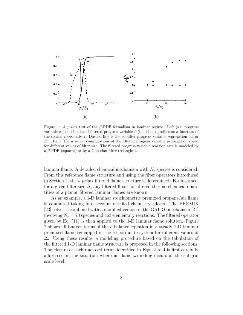
conducting a priori tests on a 1-D stoichiometric freely propagating laminarpremixed propane/air flame computed with PREMIX [20] using a modifiedversion of the GRI 3.0 mechanism [21]. The progress variable c is plottedas a function of the spatial coordinate x in Fig. 1(a). The laminar flamethickness, defined by δl = 1/ max(|dc/dx|) is approximately equal to 0.4 mm.

Introducing P , the mass weighted PDF defined by ρP = ρP , the progressvariable filtered reaction rate reads:

5

˜ωc(x) =

∫ 1

0

ωc(c)P (x, c)dc (8)

Assuming that c follows a β distribution [22]:

P (x, c) =cac−1(1 − c)bc−1

∫ 1

0cac−1(1 − c)bc−1dc

(9)

where parameters ac and bc are determined from c and the segregation factorSc = (cc − cc) / (c(1 − c)):

ac = c

(1

Sc

− 1

); bc = ac

(1

c− 1

)(10)

The knowledge of the first and second moment of the progress variableprovides the filtered reaction rate ˜ωc = ˜ωc(c, Sc). For the configuration con-sidered here, c and Sc profiles across the filtered laminar flame front arecomputed by applying a 1-D Gaussian filter F of size ∆ defined by:

F (x) =

(6

π∆2

)1/2

e−6x

2

∆2 (11)

on the detailed chemistry laminar flame solution.Favre-filtered progress variable and the segregation factor are shown in

Fig. 1(a) for a filter size of ∆ = 20δl. According to Eq. 9, the presumed

β-PDF , P (x, c), is deduced from these two quantities. The reaction rate˜ωc across the filtered flame front is then estimated from Eq. 8. Finally, theintegration of the filtered reaction rate according to Eq. 7 gives an a priori

estimation of the filtered flame front propagation speed S∆. The ratio S∆/S0l

(square symbols) is plotted as a function of the ratio ∆/δl in Fig. 1(b). When∆/δl < 1 the effect of the β-PDF on the flame structure is moderate and thepropagation speed is correctly reproduced. However when the filter size islarger than the flame front, as in LES practical situations, the propagationspeed of the filtered progress variable is largely over-estimated by the pre-sumed β function up to a factor of 2.5. In fact, the β-PDF is not relevantwhen subgrid scale wrinkling is resolved.

6

A solution to propagate a flame front at the correct speed is to artificiallythicken the reaction zone. In the Thickened Flame model for LES (TFLES)[7, 8], both reaction rate and diffusion fluxes are affected in order to ensure acorrect propagation of the flame front. However the structure of the thickenedflame front does not correspond to the filtered flame front.

An alternative to presumed PDF formalism and TFLES is to directlyemploy a normalized filter function F (x) to estimate the filtered reactionrate. Then the filtered reaction rate reads:

˜ωc(x) =1

ρ

∫ +∞

−∞

ρ(x′)ωc(x′)F (x − x′)dx′ , (12)

Since by definition, F (x) satisfies∫ +∞

−∞F (x)dx = 1, Eq. 7 is then always

satisfied:

ρ0S∆ =

∫ +∞

−∞

ρ˜ωc(x)dx (13)

=

∫ +∞

−∞

∫ +∞

−∞

ρ(x′)ωc(x′)F (x − x′)dx′dx (14)

=

∫ +∞

−∞

ρ(x′)ωc(x′)

[∫ +∞

−∞

F (x − x′)dx

]dx′ (15)

=

∫ +∞

−∞

ρ(x′)ωc(x′)dx′ (16)

= ρ0S0l (17)

This property is verified in Fig. 1(b) where the propagation speed S∆ of thefiltered flame, is a priori computed using Eqs. 11 and 12.

By taking advantages of this property, a model is proposed in Section 4 toensure the correct propagation of filtered laminar flame front. The closure ofunknown terms is carefully addressed and the model is tested on 1-D filteredflame configurations. This approach is extended to turbulent regimes wheresubgrid flame wrinkling occurs at the subgrid scale level in Section 5 by theintroduction of the subgrid flame wrinkling factor.

4. Filtered laminar premixed flames modeling

4.1. Modeling

The flame structure in the direction n normal to the flame front is as-sumed identical to the structure of a planar 1-D freely propagating premixed

7

(a) (b)

Figure 1: A priori test of the β-PDF formalism in laminar regime. Left (a): progressvariable c (solid line) and filtered progress variable c (bold line) profiles as a function ofthe spatial coordinate x. Dashed line is the subfilter progress variable segregation factorSc. Right (b): a priori computations of the filtered progress variable propagation speedfor different values of filter size. The filtered progress variable reaction rate is modeled bya β-PDF (squares) or by a Gaussian filter (triangles).

laminar flame. A detailed chemical mechanism with Ns species is considered.From this reference flame structure and using the filter operators introducedin Section 2, the a priori filtered flame structure is determined. For instance,for a given filter size ∆, any filtered fluxes or filtered thermo-chemical quan-tities of a planar filtered laminar flames are known.

As an example, a 1-D laminar stoichiometric premixed propane/air flameis computed taking into account detailed chemistry effects. The PREMIX[23] solver is combined with a modified version of the GRI 3.0 mechanism [21]involving Ns = 70 species and 463 elementary reactions. The filtered operatorgiven by Eq. (11) is then applied to the 1-D laminar flame solution. Figure2 shows all budget terms of the c balance equation in a steady 1-D laminarpremixed flame remapped in the c coordinate system for different values of∆. Using these results, a modeling procedure based on the tabulation ofthe filtered 1-D laminar flame structure is proposed in the following sections.The closure of each unclosed terms identified in Eqs. 2 to 4 is first carefullyaddressed in the situation where no flame wrinkling occurs at the subgridscale level.

8

(a) ∆ = 0.2δl (b) ∆ = 1δl

(c) ∆ = 5δl (d) ∆ = 25δl

Figure 2: Budget terms (in kg.m−3.s−1) as a function of c of the filtered progress variablebalance equation of a steady 1-D laminar planar filtered premixed flame for different values

of filter size ∆ : ∂ρeu∗

ec∗

∂x∗= ∂

∂x∗

(ρD ∂c∗

∂x∗

)− ∂

∂x∗

(ρu∗c∗ − ρu∗c∗

)+ ρ˜ω∗

c . — : ∂ρeu∗ ec∗

∂x∗. :

∂∂x∗

(ρD ∂c∗

∂x∗

). : − ∂

∂x∗

(ρu∗c∗ − ρu∗c∗

). N: ρ˜ω∗

c . ♦: ∂∂x∗

(ρD ∂ec∗

∂x∗

). Terms are plotted

in the c coordinate for different values of filter size ∆.

9

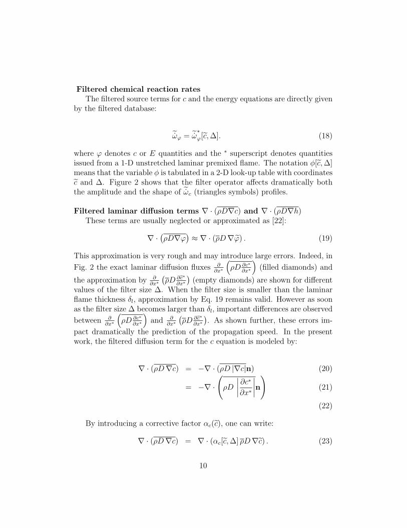
Filtered chemical reaction rates

The filtered source terms for c and the energy equations are directly givenby the filtered database:

˜ωϕ = ˜ω∗

ϕ[c, ∆]. (18)

where ϕ denotes c or E quantities and the ∗ superscript denotes quantitiesissued from a 1-D unstretched laminar premixed flame. The notation φ[c, ∆]means that the variable φ is tabulated in a 2-D look-up table with coordinatesc and ∆. Figure 2 shows that the filter operator affects dramatically boththe amplitude and the shape of ˜ωc (triangles symbols) profiles.

Filtered laminar diffusion terms ∇ · (ρD∇c) and ∇ · (ρD∇h)These terms are usually neglected or approximated as [22]:

∇ ·(ρD∇ϕ

)≈ ∇ · (ρD∇ϕ) . (19)

This approximation is very rough and may introduce large errors. Indeed, in

Fig. 2 the exact laminar diffusion fluxes ∂∂x∗

(ρD ∂c∗

∂x∗

)(filled diamonds) and

the approximation by ∂∂x∗

(ρD ∂ec∗

∂x∗

)(empty diamonds) are shown for different

values of the filter size ∆. When the filter size is smaller than the laminarflame thickness δl, approximation by Eq. 19 remains valid. However as soonas the filter size ∆ becomes larger than δl, important differences are observed

between ∂∂x∗

(ρD ∂c∗

∂x∗

)and ∂

∂x∗

(ρD ∂ec∗

∂x∗

). As shown further, these errors im-

pact dramatically the prediction of the propagation speed. In the presentwork, the filtered diffusion term for the c equation is modeled by:

∇ · (ρD∇c) = −∇ · (ρD |∇c|n) (20)

= −∇ ·

(ρD

∣∣∣∣∂c∗

∂x∗

∣∣∣∣n)

(21)

(22)

By introducing a corrective factor αc(c), one can write:

∇ · (ρD∇c) = ∇ · (αc[c, ∆] ρD∇c) . (23)

10

The normal to the flame front n = −∇c/|∇c| points into the fresh reactants.The correction factor αc(c) is defined as:

αc[c, ∆] =

ρD

∣∣∣∣∂c∗

∂x∗

∣∣∣∣

ρD

∣∣∣∣∂c∗

∂x∗

∣∣∣∣. (24)

The quantity αc[c, ∆] is estimated from the 1-D filtered flame solution andis tabulated as a function of c for a given value of filter size ∆.

Similarly, the energy-filtered laminar diffusion term is written as:

∇ · (ρD∇hs) = ∇ ·(αE([c, ∆]) ρD∇hs

), (25)

where the correction factor αE[c, ∆] is defined as:

αE[c, ∆] =

ρD

∣∣∣∣∂h∗

s

∂x∗

∣∣∣∣

ρD

∣∣∣∣∣∂h∗

s

∂x∗

∣∣∣∣∣

. (26)

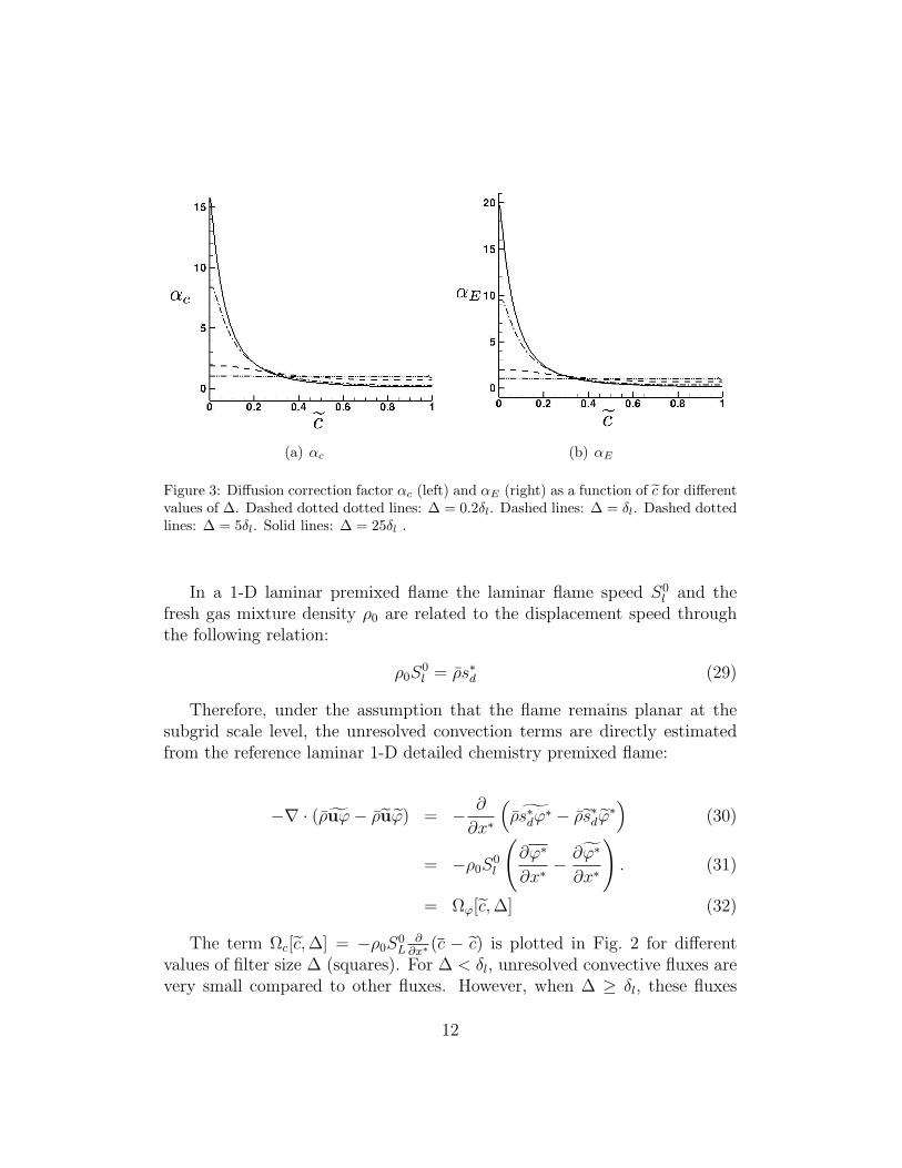
The correction factors αc[c, ∆] and αE[c, ∆] are plotted in Fig. 3 for differ-ent values of filter size ∆. For small values of ∆, as αc[c, ∆] remains constantand close to 1, effects on the laminar diffusion fluxes modeling will be negli-gible. However, the profiles present strong variations in terms of c when thefilter size ∆ is larger than δl.

Unresolved convection terms −∇ · (ρuϕ − ρuϕ)The displacement speed sd, measuring the flame front local speed relative

to the flow, i.e. the difference between the absolute flow velocity u and theabsolute flame front speed w, is first introduced:

u = w + sd (27)

The filtered flame front speed w remains constant across the flame brush(w = w = w), therefore after replacing the flow velocity by relation 27, thesubgrid scale convection term then reads:

−∇ · (ρuϕ − ρuϕ) = −∇ · (ρsdϕ − ρsdϕ) (28)

11

(a) αc (b) αE

Figure 3: Diffusion correction factor αc (left) and αE (right) as a function of c for differentvalues of ∆. Dashed dotted dotted lines: ∆ = 0.2δl. Dashed lines: ∆ = δl. Dashed dottedlines: ∆ = 5δl. Solid lines: ∆ = 25δl .

In a 1-D laminar premixed flame the laminar flame speed S0l and the

fresh gas mixture density ρ0 are related to the displacement speed throughthe following relation:

ρ0S0l = ρs∗d (29)

Therefore, under the assumption that the flame remains planar at thesubgrid scale level, the unresolved convection terms are directly estimatedfrom the reference laminar 1-D detailed chemistry premixed flame:

−∇ · (ρuϕ − ρuϕ) = −∂

∂x∗

(ρs∗dϕ

∗ − ρs∗dϕ∗

)(30)

= −ρ0S0l

(∂ϕ∗

∂x∗−

∂ϕ∗

∂x∗

). (31)

= Ωϕ[c, ∆] (32)

The term Ωc[c, ∆] = −ρ0S0L

∂∂x∗

(c − c) is plotted in Fig. 2 for differentvalues of filter size ∆ (squares). For ∆ < δl, unresolved convective fluxes arevery small compared to other fluxes. However, when ∆ ≥ δl, these fluxes

12

become important and are counter-gradient type. Note that this result is inagreement with recent experiments [24]. The quantity Ωϕ[c, ∆], estimatedfrom the 1-D filtered flame solution, is then tabulated as a function of c and∆. In practice, as the unresolved convective terms are modeled as a sourceterm, only the sum Σϕ[c, ∆] = Ωϕ[c, ∆] + ˜ωϕ[c, ∆] is stored in the filtereddatabase where φ denotes c or E quantities.

Pressure term

In a similar way, the pressure term in the energy equation (Eq. 4) iswritten as:

−∇ · (Puδ) = −∇ · (P uδ) −(∇ · (Puδ) −∇ · (P uδ)

)(33)

= −∇ · (P uδ) −(∇ · (ρrTuδ) −∇ · (ρrT uδ)

)(34)

= −∇ · (P u δ) + Ωp[c, ∆] (35)

with

Ωp[c, ∆] = −ρ0 S0l

(∂(rT ∗)

∂x∗−

∂(rT ∗)

∂x∗

). (36)

Momentum equations

Unclosed terms in the filtered momentum equations may be modeledfollowing the same approach. The subgrid scale convection term is writtenas:

−∇ · (ρuu − ρuu) =∂

∂x∗

(ρs∗ds

∗

d − ρsd∗sd

∗

)n (37)

= ρ0S0l

(∂sd

∗

∂x∗−

∂sd∗

∂x∗

)n (38)

= Ωu[c, ∆]n (39)

The strain tensor is expressed by:

∇ · τ = ∇ · (αu[c, ∆]τ) with αu[c, ∆] =τ ∗

τ ∗. (40)

where τ is defined as:

τ = µ

(∇u + (∇u)T −

2

3(∇ · u)δ

)(41)

13

However, as shown further, the influence of these terms is moderate and canbe neglected.

4.2. Summary of the model equations

The momentum, the progress variable and the energy equations are mod-eled as:

∂ρu

∂t+ ∇ · (ρuu) = −∇P + ∇ · (αu[c, ∆]τ) + Ωu(c)n (42)

∂ρc

∂t+ ∇ · (ρuc) = ∇ · (αc[c, ∆] ρD∇c) + Σc[c, ∆] (43)

∂ρE

∂t+ ∇ · (ρuE) = −∇ ·

(P u δ

)+ Ωp[c, ∆] + ∇ · (τ u)

+∇ ·(αE[c, ∆] ρD∇hs

)+ ΣE[c, ∆] (44)

These equations are implemented in the compressible LES code AVBP[25]. The third-order finite element scheme TTGC [26] is used. Boundaryconditions are prescribed using Navier-Stokes Characteristic Boundary Con-ditions [27].

The sum of filtered chemical reactions rates and the subgrid scales fluxesΣϕ = Ωϕ+ρ˜ωϕ and the diffusion fluxes correction factors αϕ are estimated af-ter filtering a 1-D laminar stoichiometric premixed propane/air flame. Thesequantities are stored in a look-up table as a function of c and ∆.

4.3. 1-D laminar premixed flame simulations

Filtered steady 1-D laminar flames are computed to verify the abilityof the present model to reproduce both the correct flame front propagationspeed and the filtered flame structure. Computations are performed on uni-form meshes with a grid spacing of ∆x. A parametric study is conducted fordifferent filter sizes relative to the laminar flame thickness. For each case,a reference solution is obtained by filtering the 1-D laminar premixed flamedetailed chemistry solution. The simulations are initialized with the refer-ence solution and the overall physical time for each run is trun = 50 δec /S0

l ,where δec = 1/ max(| ∂ec

∂x|) is an estimation of the filtered flame thickness.

A comparison between the numerical solutions on uniform mesh (solidlines) and the reference solution (dashed line) with δec/∆x = 50 and for dif-ferent values of ∆/δl is first shown in Fig. 4. The predicted filtered progress

14

Figure 4: Filtered 1-D premixed flame solutions. Filtered progress variable (solid) com-pared to the reference solution (dashed) for ∆/δl = 2, 10 and 20.

variable profiles match the reference solution for all the filter size values. Fig-ure 5(a) shows that the predicted filtered front propagation speed S∆(squaresymbols) remains very close to the reference laminar flame speed for vari-ous values of ∆/δl. The triangular symbol in Fig. 5(a) represents simulationresults with the approximation given by Eq. (19), i.e., αϕ = 1. This roughassumption leads to an under-prediction by a factor of 3 of the flame frontpropagation speed.

An important information for premixed combustion LES is the minimalnumber of grid points required to capture the filtered flame front withoutintroducing numerical artifacts. The filtered flame front propagation speedis plotted as a function of the mesh resolution ∆x in Fig.5(b). The flamespeed is recovered with a good approximation for δec/∆x ≥ 5. Below thislimit, numerical errors become important and the filtered flame front does notpropagate at the correct speed. Then, for numerical reasons, the filter shouldbe at least 5 times larger than the mesh size. Note that even approaches basedon level-set transport that use sophisticated numerical methods to track theflame front position also require to filter the flame front at a scale larger thanthe mesh size in order to resolve density gradients [15].

15

(a) δec/∆x = 50 (b) ∆/δl = 20

Figure 5: Predicted flame speed as a function of ∆/δl (left) and δec/∆x (right). Squaresymbols are the complete model solution and the triangle symbol is the solution withαϕ = 1.

Finally, a simulation has been performed without considering the filteringeffect on the momentum equations (Eq. 42), i.e., with αu = 1 and Ωu = 0 andis compared with the complete model solution in Fig. 6. For both simulations,density as well as velocity profiles match perfectly. In fact, the induceddifferences are transfered to the pressure that becomes a macro-pressure. Asthis macro-pressure remains very close to the static pressure, effects on thethermodynamic state are very limited. Then, in order to simplify the modelimplementation in 3-D configurations, the contribution corresponding to thefiltering of a laminar flame in the momentum equation will be neglected.

5. Filtered turbulent premixed flames modeling

In practical LES of turbulent combustion, turbulence may cause flamefront wrinkling at the subgrid scale level. Here, a strategy is proposed toextend the previously described model to such situations.

5.1. Modeling

Turbulent structures induce flame wrinkling that increases the flame sur-face area at the subgrid scale. As a consequence the filtered flame front

16

Figure 6: Filtered 1-D premixed flame solutions. Effects of the flame filter in the momen-tum equation. Solid: αu = 1 and Ωu = 0. Symbols: αu(c) and Ωu(c) from the filtereddatabase.

propagates at a subgrid scale turbulent flame speed St [22] related to thelaminar flame speed through the flame wrinkling factor Ξ = St/S

0l .

The model developed here ensures that the filtered flame front propagatesat the turbulent flame speed St. The filtered flame thickness is assumed tobe only related to the filter size ∆ and is not altered by small-scale eddies.

Then, the filtered progress variable turbulent reaction rate is modeled by:

ωct= Ξ . ω

∗

c [c, ∆] (45)

and the turbulent diffusion term is expressed as follows:

Ωct= − (∇ · (ρuc − ρuc))

t= Ξ Ωc[c, ∆] + (Ξ − 1)∇ · (αc[c, ∆] ρD∇c)

(46)

The first term on the r.h.s corresponds to the thermal expansion and thesecond one models the unresolved turbulent fluxes. This formulation corre-sponds to multiply diffusion and source terms by the flame wrinkling factorin the laminar flame balance equation and then ensures that the unstretchedfiltered flame front propagates at the turbulent flame speed St = ΞS0

l in thenormal direction.

17

5.2. Summary of the model equations

To summarize, momentum, progress variable and energy equations forthis new model called Filtered Tabulated Chemistry for LES (F-TACLES)can be written as follows:

∂ρu

∂t+ ∇ · (ρuu) = −∇P + ∇ · τ + ∇ · τ t (47)

∂ρc

∂t+ ∇ · (ρuc) = Ξ∇ · (αc[c, ∆] ρD∇c) + ΞΣc[c, ∆] (48)

∂ρE

∂t+ ∇ · (ρuE) = −∇ · (P u δ) + ΞΩp[c, ∆] + ∇ · (τ u)

+Ξ∇ ·(αE[c, ∆] ρD∇hs

)+ ΞΣE[c, ∆]. (49)

Note that here the effect of the flame filter ∆ on the momentum equations isneglected and the subgrid scale turbulent fluxes ∇· τ t are modeled using theSmagorinsky model. Different alternatives exist to estimate the subgrid flamewrinkling factor that appears in Eqs 48 and 49. It can be either estimatedfrom analytical models [8, 14, 28, 29] or from the solution of a surface densitybalance equation [30, 31].

5.3. Large Eddy Simulation of a swirled premixed burner

The proposed method is applied to the simulation of the complex PREC-CINSTA swirled burner experimentally investigated by Meier et al. [32]. Thegeometry, shown in Fig. 7, derives from an aeronautical combustion device.It features a plenum, a swirl-injector and a combustion chamber. Detailsof the burner geometry and of the measurement can be found in Ref. [32].Different modeling strategies for LES have been used to numerically investi-gate this configuration : an LES of the combustor using the thickened flamemodel and a two-step mechanism has been first performed by Roux et al..[33]. Moureau et al. [34] used this configuration to validate a new level-setalgorithm to track the flame front position. Recently, Galpin et al. [16] per-formed the LES of this lean premixed burner by using a presumed β-PDF tocouple a thermo-chemical look-up table with the filtered flow equations.

The operating conditions chosen in the present study correspond to anair mass flow rate of 12.2 g/s and to a methane mass flow rate of 0.6 g/s. Inthe experiment, air and methane are injected separately in the plenum inlet,however in the present simulation the mixing is assumed to be fast enough

18

to burn a perfect mixing of oxidizer and fuel in the combustion chamber.Thus methane injection is not taken into account and a methane/air mixturecharacterized by an equivalence ratio of 0.83 is injected at the plenum inlet.These conditions correspond to a stable regime where laser Raman scatteringhas been performed, allowing comparison between predicted and measuredthermo-chemical quantities such as temperature and species mass fractions.

The boundary conditions and the computational geometry have been al-ready described in [33]. The mesh used to perform the computation is un-structured and made of 12.7 millions elements. The third-order finite elementscheme TTGC [26] is retained. For building-up the chemical look-up table,a 1-D laminar methane/air flame is first computed for an equivalence ratioequal to 0.83 using the GRI 3.0 mechanism [21]. Then, according to the mod-eling procedure discussed previously, this laminar flame solution is filteredby the Gaussian function defined by Eq. 11.

Note that, as the mesh considered here is almost uniform in the filteredflame front region, an unique filter width ∆ is considered. In order to ensurea sufficient meshing of the filtered flame front, the filter width has been setto ∆ = 20δl. The progress variable is defined by c = YCO2

/Y eqCO2

, where Y eqCO2

is the equilibrium CO2 mass fraction in the fully burnt gases. The filteredquantities required by the model: Σc[c, ∆], αc[c, ∆], Ωp[c, ∆], ΣE[c, ∆] andαE[c, ∆] are then tabulated as a function of c for ∆ = 20δl. For stronglynon-uniform meshes this procedure is not optimized and could lead to over-refined or under-refined flame front regions. Then, an additional coordinate,the filter width, can be easily considered when computing the look-up table.

Following the system of equations 47-49, this new model F-TACLES hasbeen implemented into the compressible LES code AVBP [25]. The subgridflame wrinkling factor Ξ is estimated from the analytical model developedby Colin et al. [8]. Mean and resolved Root Mean Square (RMS) quantitiesare computed by time averaging LES solutions over a physical time thatcorrespond to 6 flow-through times based on the fresh gas inlet velocity. Meantemperature and CO2 mass fractions are plotted on Figs. 8 (top) and 9 (top),respectively. A very good agreement is observed between experimental andnumerical profiles, which demonstrated that the correct flame angle and meanflame thickness are reproduced by the model. Because heat losses have notbeen considered when generating the chemical database and in the numericalsimulation, the LES slightly over-estimates the temperature profiles close tothe combustion chamber wall, in the outer recirculation zone for x < 20 mmand at a distance larger than 20mm from the jet axis. Note that heat losses

19

effects on the flame structure can be taken into account with the addition ofthe enthalpy as a control parameter of the chemistry tabulation [3, 6].

Figs. 8 (bottom) and 9 (bottom) show a comparison between resolvedLES RMS and measured RMS of the temperature and the CO2 mass frac-tion, respectively. As the plotted LES RMS does not include the subgridscale RMS, conclusions regarding the model performance in terms of flameturbulence interactions are more difficult. However, it is observed that LESRMS remains lower than measured RMS, as expected from theory.

As all thermo-chemical variables are related to c, the post-processing ofthe filtered progress variable solution with the filtered chemical databaseallows to access all chemical species. As an example, Fig. 10(a) shows 2-Dcontours of c used to estimate HCO mass fraction plotted in Fig. 10(b).

Finally, Fig. 11 indicates the flame position in the Pitsch LES regimediagram for turbulent premixed combustion [17], where the ratio ∆/δl isexpressed as a function of the Karlovitz number Ka in logarithmic scale.The Karlovitz number is related in LES to the subgrid velocity fluctuationsv′

∆ and laminar flame scales [17]:

Ka2 =δl

S0l3ε =

v′

∆

S0l

δl

∆(50)

where ε is the kinetic energy transfer rate. The subgrid velocity fluctua-tions are computed as follows:

v′

∆ =µt

ρCk∆√

3/2(51)

where the turbulent viscosity µt is estimated from Smagorinsky model. ForKa < 1, combustion takes place in the corrugated flame regime while thethin reaction zone regime is observed when Ka > 1. Computational nodeslocated in the filtered flame front are considered, i.e. for 0.01 < c < 0.99, andare plotted in the LES diagram (horizontal thick solid black line in Fig. 11).As a a unique filter width ∆ is considered in the present simulation, thescatter plot reduced to the line ∆/δl = 20. The smallest size of the flamewrinkling is given by the Gibson length [11]:

∆

lG=

v′

∆

S0l

(52)

The substitution of Eq. 52 into Eq. 50 shows that ∆ = lG condition cor-responds to ∆/δl = Ka−2 represented by a line of slope −2 in the LES

20

Figure 7: LES of Preccinsta with F-TACLES turbulent combustion model. The compu-tational domain features the plenum, the swirl-injector and the combustion chamber. Aninstantaneous view of the filtered flame front iso-surface (c=0.8) is shown.

diagram (Fig. 11). In the corrugated flame regime, when the filter width be-comes smaller than the Gibson length, the subgrid velocity fluctuation v′

∆ issmaller than the laminar flame speed S0

l . In such cases, the flame wrinklingis fully resolved at the LES filter scale. At the opposite, on the right side ofthe lG = ∆ line, subgrid scale wrinkling exists and will impact the filteredflame front propagation speed S∆. The node distribution versus the Karlovitznumber is plotted in Fig. 12. First, it can be observed that most of the pointsare located in the corrugated flame regime (Ka < 1). The chemical flamestructure remains therefore laminar as assumed in the present model. Sec-ondly, for a substantial area of the flame surface ( about 30 %), the Gibsonlength lG is larger than the filter width and consequently the flame wrinklingis fully resolved. With future increase of computational power, as meshes willbe finer, this trend should be emphasized. It demonstrates the crucial needof ensuring a proper propagation of the laminar flame front when deriving aturbulent combustion model.

6. Conclusion

A new modeling strategy called Filtered Tabulated Chemistry for LES (F-TACLES) has been developed to introduce tabulated chemistry methods inpremixed combustion LES. A filtered 1-D laminar premixed flame is used tobuild a filtered chemical look-up table. The model performances are demon-strated on 1-D filtered laminar flame computations. Finally the proposedstrategy has been applied to perform a 3-D simulation of a swirled turbulent

21

x = 15mm2000

-40

-20

0

20

40

x = 20mm2000

-40

-20

0

20

40

x = 30mm2000

-40

-20

0

20

40

x = 40mm2000

-40

-20

0

20

40

x = 60mm2000

-40

-20

0

20

40

x = 10mm2000

-40

-20

0

20

40

x = 6mm

Distancefromaxis(mm)

2000

-40

-20

0

20

40

x = 30mm0.05 0.1

-40

-20

0

20

40

x = 15mm500

-40

-20

0

20

40

x = 10mm0 500

-40

-20

0

20

40

x = 20mm500

-40

-20

0

20

40

x = 30mm500

-40

-20

0

20

40

x = 40mm500

-40

-20

0

20

40

x = 60mm500

-40

-20

0

20

40

x = 6mm

Distancefromaxis(mm)

0 500

-40

-20

0

20

40

Figure 8: Mean (top) and RMS (bottom) of temperature, case φ = 0.83. Symbols:measurements. Lines: simulation with F-TACLES. x = 0 matches the swirler exit.

22

x = 6mm

Distancefromaxis(mm)

0.05 0.1

-40

-20

0

20

40

x = 10mm0.05 0.1

-40

-20

0

20

40

x = 15mm0.05 0.1

-40

-20

0

20

40

x = 20mm0.05 0.1

-40

-20

0

20

40

x = 30mm0.05 0.1

-40

-20

0

20

40

x = 30mm0.05 0.1

-40

-20

0

20

40

x = 40mm0.05 0.1

-40

-20

0

20

40

x = 60mm0.05 0.1

-40

-20

0

20

40

x = 30mm0.05 0.1

-40

-20

0

20

40

x = 10mm0 0.02 0.04

-40

-20

0

20

40

x = 15mm0 0.02 0.04

-40

-20

0

20

40

x = 60mm0 0.02 0.04

-40

-20

0

20

40

x = 30mm0 0.02 0.04

-40

-20

0

20

40

x = 6mm

Distancefromaxis(mm)

0 0.02 0.04

-40

-20

0

20

40

x = 20mm0 0.02 0.04

-40

-20

0

20

40

x = 40mm0 0.02 0.04

-40

-20

0

20

40

Figure 9: Mean (top) and RMS (bottom) of CO2 mass fraction, case φ = 0.83. Symbols:measurements. Lines: simulation with F-TACLES. x = 0 matches the swirler exit.

23

(a) c

(b) YHCO

Figure 10: 2-D instantaneous view of c and YHCO.

premixed flame. Good agreement between the numerical simulation and theexperiments is observed.

7. Acknowledgments

This work was supported by the ANR-07-CIS7-008-04 Grant of the FrenchMinistry of Research. We are grateful to the CERFACS (Toulouse, France)combustion team for providing the PRECCINSTA burner geometry. Theauthors warmly acknowledge the support of the 2008 Summer Program of theCenter for Turbulence Research (Stanford University - NASA Ames) duringwhich this work was initiated. This work was granted access to the HPCresources of IDRIS under the allocation 2009-i2009020164 made by GENCI(Grand Equipement National de Calcul Intensif)

24

Figure 11: LES regime diagram for turbulent premixed combustion. The thick solid blackline represent the range covered by the Preccinsta flame simulation.

25

Figure 12: Node distribution versus the Karlovitz number. Only nodes located into thefiltered flame front have been considered, i.e. for 0.01 < c < 0.99.

26

References

[1] U. Maas, S. Pope, Simplifying chemical kinetics: Intrinsic low-dimensional manifolds in composition space, Combust. Flame 88 (1992)239–264.

[2] O. Gicquel, N. Darabiha, D. Thevenin, Laminar premixed hydrogen /air counterflow flame simulations using flame prolongation of ildm withdifferential diffusion, in: The Proceedings of the Twenty-Eighth Sympo-sium (Int.) on combustion. The Combustion Institute, Pittsburgh, 2000,pp. 1901–1908.

[3] B. Fiorina, R. Baron, O. Gicquel, D. Thevenin, S. Carpentier, N. Dara-biha, Modelling non-adiabatic partially-premixed flames using flameprolongation of ildm, Combustion Theory and Modelling 7 (2003) 449–470.

[4] J. A. van Oijen, F. A. Lammers, L. P. H. de Goey, Modelling of com-plex premixed burner systems by using flamelet-generated manifolds,Combust. Flame 127 (3) (2001) 2124–2134.

[5] L. Vervisch, R. Haugel, P. Domingo, M. Rullaud, Three facets of tur-bulent combustion modelling: Dns of premixed flame, les of lifted non-premixed v-flame and rans of jet-flame, J. of Turbulence 5 (4) (2004)1–36.

[6] B. Fiorina, O. Gicquel, L. Vervisch, S. Carpentier, N. Darabiha, Pre-mixed turbulent combustion modelling using tabulated chemistry andpdf, Proc. Combust. Inst. 30 (2005) 867–874.

[7] T. D. Butler, P. J. O’Rourke, A numerical method for two-dimensionalunsteady reacting flows., Proceedings of the 16th Symp. (Int.) on Com-bustion. The Combustion Institute: Pittsburgh, Penn. (1977) 1503–1515.

[8] O. Colin, F. Ducros, D. Veynante, T. Poinsot, A thickened flame modelfor large eddy simulations of turbulent premixed combustion, Physics ofFluids 12 (7) (2000) 1843–1863.

27

[9] M. Boger, D. Veynante, H. Boughanem, A. Trouve, Direct numericalsimulation analysis of flame surface density concept for large eddy sim-ulation of turbulent premixed combustion, in: Twenty-Seventh Sym-posium (Int.) on Combustion. The Combustion Institute: Pittsburgh,Penn., 1998, pp. 917 – 925.

[10] C. Duwig, Study of a filtered flamelet formulation for large eddy simu-lation of premixed turbulent flames, Flow Turbulence and Combustion79 (4) (2007) 433–454.

[11] N. Peters, Turbulent Combustion, Cambridge University Press, 2000.

[12] S. Menon, W. Jou, Large eddy simulations of combustion instability inan axisymetric ramjet combustor, Combust. Sci. and Tech. 75 (1991)53–72.

[13] V.-K. Chakravarthy, S. Menon, Subgrid modeling of turbulent premixedflames in the flamelet regime, Flow, Turbulence and Combustion 65(2000) 133–161.

[14] H. Pitsch, A consistent level set formulation for large-eddy simulationof premixed turbulent combustion, Combust. Flame 143 (4) (2005) 587–598.

[15] V. Moureau, B. Fiorina, H. Pitsch, A level set formulation for premixedcombustion les considering the turbulent flame structure, combust. andFlame 156 (4) (2009) 801–812.

[16] J. Galpin, A. Naudin, L. Vervisch, C. Angelberger, O. Colin,P. Domingo, Large-eddy simulation of a fuel-lean premixed turbulentswirl-burner, Combust. Flame 155 (2008) 247–266.

[17] H. Pitsch, Large-eddy simulation of turbulent combustion, Ann. Rev.Fluid Mech. 38 (2006) 453–482.

[18] E. R. Hawkes, R. S. Cant, Physical and numerical realizability require-ments for flame surface denisty approaches and reynolds averaged sim-ulation of premixed turbulent combustion, Combust. Theory and Mod-elling 5 (2001) 699–720.

28

[19] A. W. Vreman, J. A. van Oijen, L. P. H. de Goey, R. J. M. Bastiaans,Subgrid scale modeling in large eddy simulation of turbulent combustionusing premixed flamelet chemistry, Flow, Turbulence and Combustion82 (2009) 511–535.

[20] R. J. Kee, J. F. Grcar, M. D. Smooke, J. A. Miller, A fortran programfor modelling steady laminar one-dimensional premixed flames, Tech.Rep. SAND85-8240-UC-401, Sandia National Laboratories (1985).

[21] http://www.me.berkeley.edu/gri-mech/.

[22] T. Poinsot, D. Veynante, Theoretical and Numerical Combustion,R. T. Edwards, Inc., 2005.

[23] R. J. Kee, J. F. Grcar, M. D. Smooke, J. A. Miller, A fortran programfor modelling steady laminar one-dimensional premixed flames, Tech.rep., Sandia National Laboratories (1992).

[24] S. Pfadler, J. Kerl, F. Beyrau, A. Leipertz, A. Sadiki, J. Scheuerlein,F. Dinkelacker, Direct evaluation of the subgrid scale scalar flux in tur-bulent premixed flames with conditioned dual-plane stereo piv, Proceed-ings of the Combustion Institute 32 (2) (2009) 1723 – 1730.

[25] Avbp code : www.cerfacs.fr/cfd/avbp code.php and www.cerfacs.fr/cfd/cfdpublications.html.

[26] O. Colin, M. Rudgyard, Development of high-order taylor-galerkinschemes for unsteady calculations, J. Comput. Phys. 162 (2) (2000) 338–371.

[27] T. Poinsot, S. K. Lele, Boundary conditions for direct simulations ofcompressible viscous flows, J. Comput. Phys. 1 (101) (1992) 104–129.

[28] F. Charlette, C. Meneveau, D. Veynante, A power-law flame wrinklingmodel for les of premixed turbulent combustion, part i: non-dynamicformulation, Combust. Flame 131 (1/2) (2002) 159–180.

[29] F. Charlette, C. Meneveau, D. Veynante, A power-law flame wrinklingmodel for les of premixed turbulent combustion, part ii: dynamic for-mulation, Combust. Flame 131 (1/2) (2002) 181–197.

29

[30] E. R. Hawkes, R. S. Cant, A flame surface density approach to large-eddy simulation of premixed turbulent combustion, Proc. Combust. Inst28 (2000) 51–58.

[31] S. Richard, O. Colin, O. Vermorel, A. Benkenida, C. Angelberger,D. Veynante, Towards large eddy simulation of combustion in sparkignition engines, Proc. Combust. Inst 31 (2007) 3059–3066.

[32] W. Meier, P. Weigand, X. Duan, R. Giezendanner-Thoben, Detailedcharacterization of the dynamics of thermoacoustic pulsations in a leanpremixed swirl flame, Combustion and Flame 150 (1-2) (2007) 2 – 26.

[33] S. Roux, G. Lartigue, T. Poinsot, U. Meier, C. Berat, Studies of meanand unsteady flow in a swirled combustor using experiments, acousticanalysis, and large eddy simulations, Combustion and Flame 141 (1-2)(2005) 40 – 54.

[34] V. Moureau, P. Minot, H. Pitsch, C. Berat, A ghost-fluid method forlarge-eddy simulations of premixed combustion in complex geometries,Journal of Computational Physics 221 (2) (2007) 600 – 614.

30