DEPRESSION OR PRICE CONTROLS: A FICTITIOUS DILEMMA FOR ANTI-INFLATION POLICY

Roy H. Webb

After rising by more than 13 percent in 1979, the

growth rate of the Consumer Price Index has further

increased in the first months of 1980. Consequently,

attention is being directed toward proposals for wage-

price restraint. Among the proposals that have been

mentioned are a wage and price freeze (as in August

1971), a mandatory control program (similar to

Phase II of the Nixon-era controls), or some system

of tax incentives and penalties designed to slow wage

and price increases. The latter system is often re-

ferred to as a Tax-Based Incomes Policy, or TIP.

The Argument for Restraint Whatever the exact form, wage-price restraint has well-known draw- backs: (1) it may not be effective, and (2) if effec- tive, it can do severe damage to the economy (see, for example, [10]). Advocates of controls, however, argue that the costs of controls are outweighed by the costs of the alternative anti-inflation policy, that of totally relying on monetary and fiscal restraint. Arthur Schlesinger, for example, recently argued,

[T]he prospect of depression is the economic re- ality behind Carter’s anti-inflation program... In the long run, recession will indeed slow the rate of inflation. But at what social and human cost? . . . [T]he worst recession in nearly 40 years, wide- spread unemployment and considerable human an- guish . . . is . . . peanuts compared to what would be required to bring down the 20+% inflation rate Mr. Carter is giving us. . . . ‘The reserve army of the unemployed will eventually squeeze inflation out of the system,’ the economist Francis Bator has aptly commented ‘ if it doesn’t trigger a social revolution first.’ The Carter-Volker policy . . . is one of enormously high risk to the stability of our political as well as of our economic system. It offers a future of bitter unemployment, accom- panied by a very gradual reduction of inflation and by very dangerous intensification of social tension and class hostility. [9]

Evidence that monetary and fiscal restraint would

produce a severe, prolonged recession is provided by

econometric simulations. After evaluating simula-

tions from six econometric models, Arthur Okun

recently found, “. . . [T]he average estimate of the

cost of a 1 point reduction in the basic inflation rate

is 10 percent of a year’s GNP. . . .” [7] If true,

Okun’s conclusion would mean that lowering the

annual growth rate of the Consumer Price Index below 3 percent could be accomplished by a mone- tary policy restrictive enough to cause a 10 percent GNP gap for a decade. [The GNP gap is an esti- mate of the extent to which real GNP is below

normal, as would occur in a recession. In the first

quarter of 1975, the trough of a particularly severe recession, the GNP gap was about 9 percent.] That

policy would reduce output by about $250 billion annually (that is, roughly 10 percent of current GNP), or by $2.5 trillion over the decade.

The Fallacy in That Argument Policy evaluations

using econometric models such as those examined by

Okun necessarily assume that what’s past is prologue,

in that it is assumed people will respond to projected

policy decisions in exactly the same manner as they

have in the past. This seemingly innocuous assump-

tion does simplify analysis. However, previous

policy evaluations based on that assumption have often led to false conclusions.

One illustration is the income tax surcharge of 1968 and 1969. Policymakers expected the sur- charge to lower consumers’ disposable income, there- by reducing total spending for goods and services and thus dampening inflation. The Council of Eco-

nomic Advisers, for example, on the basis of the surcharge predicted a reduction in the inflation rate for 1969 to “a little more than 3 percent.” [3] Actually, the GNP implicit price deflator rose by 5.3 percent in 1969 as consumer spending accelerated, growing at a 4.6 percent rate in 1967 and an 8.7 percent rate in 1968 and 1969. As Robert Eisner has noted 141, an important reason that, consumer spending failed to weaken as many had predicted was the erroneous assumption that consumers would re- spond to a temporary tax surcharge in the same manner as they had earlier responded to permanent tax changes. In this case the past was not prologue; therefore the actual consumer reaction to the sur- charge was misjudged.

When an econometric model fails to predict the effects of an economic policy correctly, many an economist’s impulse is to tinker with the model-

FEDERAL RESERVE BANK OF RICHMOND 3

that is, to add a variable to an equation here, to add a

new equation there, to experiment with a new sta- tistical technique, etc. Robert Lucas [6] took an-

other course, however, by systematically analyzing the foundation for evaluating potential economic policies with econometric models. To understand

Lucas’s work, it will first be necessary to review the nature of econometric models.

An immense volume of statistics concerning the economy are regularly gathered. The role of eco- nomic theory is to suggest a limited number of po- tentially useful relationships among the many rela-

tions possible, Typically, one first specifies the eco- nomic choices available to individuals. The next step is to characterize the choices that best achieve

certain goals.

Consider the problem of how a household can best

allocate consumption expenditure over its members’ lifetimes, for example. Since income can limit con-

sumer spending, economic theory might suggest to the model builder that consumption should be related to income available for people to spend. This rela-

tionship could be expressed symbolically as

(1) C = θ (Y-T)

where C is national consumption expenditure, Y is national income, T is the level of taxes and θ is a parameter, that is, some number. Theory might further predict that θ is less than 1, since individuals would desire to have funds available for emergencies or retirement and would thus not consume every

penny of available income. Therefore, equation (1) states that national consumption is a fraction of national income, net of taxes. Unfortunately, theory does not often provide the exact value for a param- eter. To meet that difficulty, an econometrician esti- mates the parameter θ by statistical methods using past data.

After an estimate of θ has been made, equation (1)

could be used to predict the effect of a tax cut on con- sumption spending. As is often done in elementary

textbooks, equation (1) could also provide a basis

for a relation between national income and taxes, such as

(2) ∆ Y = - θ

∆ T. 1 - θ

In words, an increase in the level of taxes, ∆ T, θ

causes a fall in national income by the amount 1 - θ

times the tax hike. If an econometrician estimated θ as .9, for example, equation (2) would imply that a

A particularly graphic illustration of misleading

policy evaluation can be constructed by applying Okun’s 10 percent GNP gap rule to Germany in August 1922 through October 1923. Since the annual inflation rate was 300,000 percent, Okun’s rule would imply that eliminating inflation in Germany would have taken a 50 percent GNP gap for 600 centuries! Actually, the German inflation was vir- tually eliminated in 1924 with a 10 percent GNP gap. In this example the error of making an unwarranted

extrapolation is clear. It will be argued below that

1 Econometric models have many uses in addition to policy evaluation, and this critique does not challenge their efficacy for such uses. Moreover, it does not deny that changes can be imagined that would allow valid policy evaluation (for example, see [2]). Such changes are not trivial and have not been made on widely used models, however, including the models examined by Okun.

2 Lucas and other members of the New Classical school of economic thought (such as Robert Barro and Thomas Sargent) have criticized Keynesian macro-econometric models on several grounds. It is useful to focus only on the critique of econometric policy evaluation since many writings by leading Keynesian economists follow the same logic. As noted above, Eisner’s writing on the 1968-69 tax surcharge is consistent with the Lucas cri- tique. Also, Alan Blinder and Robert Solow [1] briefly made an analogous argument, that “treating the fiscal and monetary tools . . . as exogenous in the statistical sense . . . involves a specification error that all econo- metric models will continue to commit until they specify and estimate a proper reaction function for the authori- ties.”

4 ECONOMlC REVIEW, MAY/JUNE 1980

$10 billion tax increase would reduce national income

by $90 billion. It is this type of exercise that is

labeled “econometric policy evaluation.” Although

hundreds of equations and advanced statistical tech-

niques may be used, the process of econometric

policy evaluation is a mechanical extrapolation, just

as indicated by this example.

Lucas argued that this policy evaluation technique

is not logically consistent.l That is, the same eco-

nomic theory that is used to suggest equations such

as (1) also predicts that a parameter such as θ will

not be a fixed number. Instead, when economic

policy changes it will often be in an individual’s self-

interest to change his economic behavior, which in

turn may change a parameter’s value. That is

exactly what happened in 1968-69. The temporary

tax surcharge induced consumers to spend a tem- porarily higher fraction of their incomes (in equa- tions ( 1) and (2), that would mean that θ would be larger). Most econometric models therefore yielded incorrect predictions of the effect of the surcharge since parameters had been estimated from individuals’

past behavior.2

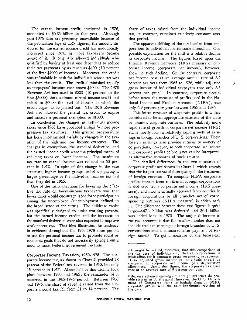
the same error is made in the well-publicized econo-

metric policy evaluations that predict excessive costs if monetary restraint is used to lower inflation.

Such forecasts rely on an equation similar to

(3) π = a π e + bE,

where π is the actual rate of inflation, π e is the extrapolated rate of inflation,3 E is excess capacity (usually measured either as above-normal unem- ployment or below-normal GNP), and a and b are parameters whose exact values are unknown. This equation, sometimes called an aggregate supply func- tion, a price equation, or a Phillips Curve, states that the actual rate of inflation is determined by the extrapolated rate of inflation and the degree of excess capacity.4 In this framework restrictive monetary policy can lower inflation only by slowing the econ- omy and causing excess capacity. By statistically estimating the value of the parameter b one can then guess the amount of excess capacity needed to lower the inflation rate by a given amount. That procedure is the basis for estimates such as those examined by Okun.

These estimates assume that the parameter b is

fixed. That assumption is questionable, since the

estimates are based on data from the post-Korean

War era-an era dominated (in fact if not in rhet-

oric) by only one monetary policy, that of frequently

shifting targets (Robert Hetzel [5] discusses this

policy, labeling it “leaning against the wind”).

Briefly, the shifting target strategy involves respond-

ing to the most pressing short-run concern, such as

interest rates, unemployment, inflation, the foreign

exchange value of the dollar, etc. The most pressing

short-run problem today, of course, will not neces-

sarily be the most pressing problem tomorrow. In

such an environment, it is not surprising that indi-

viduals have been slow to change their price or wage-

setting strategies. They have observed that monetary

restraint has previously been temporary, and that

sooner or later the focus of monetary policy changes. Such anticipations have so far proved correct. Thus

rather low estimates of the parameter b are not sur-

3 The extrapolated rate of inflation is often labeled as “the expected rate” or “the underlying rate.” Since these concepts are usually implemented as extrapolations of recent activity, the indicated expression may be more accurate.

4 It may not be easy to see how this equation results from individual decisions. Phelps [8] contains several seminal essays on this point.

prising, since individuals knew that if excess capacity should appear, the Fed would soon shift from fighting inflation to fighting unemployment.

If lower inflation were to become the dominant goal of monetary policy, the outlook could be dra- matically different. Abandoning the policy of shift- ing targets would change the context in which indi- viduals make price and wage decisions, thereby in- validating previous estimates of the parameter b in equation (3) and, consequently, the estimated cost of monetary restraint. A difficulty in implementing

such a fundamental policy change would lie in con- vincing individuals that policy has in fact been changed. Simple announcement will not suffice since anti-inflation rhetoric has accompanied recent in- creases of inflation.

Two steps toward making future announcements

more credible have recently been taken, however.

Section 108 of the Full Employment and Balanced

Growth (Humphrey-Hawkins) Act requires the Fed-

eral Reserve to announce annual targets for growth

of monetary aggregates no later than February 20 of

each year, and to explain any deviation which later

occurs. This bill gives the Fed the opportunity to

announce targets, and more importantly, the oppor-

tunity to establish a track record of meeting its stated

targets. Such a track record would increase the

responsiveness of individuals to future announce-

ments. The second step was taken when the Fed’s

operating target was changed from an interest rate

to nonborrowed bank reserves. Many economists

believe that this change gives the Fed more control

over the money supply, should such control be de-

sired.

Conclusion The foundation for wage-price re- straint is anchored in the quicksand of econometric policy evaluation. Frighteningly large estimates of the costs of monetary restraint are irrelevant if there is a credible replacement for the old policy of shifting targets. Even if such a replacement were adopted, reducing inflation would not be costless. However, a credible anti-inflation policy would lead to changes in individuals’ wage and price setting strategies which would alter the economic outcome away from that predicted by models with parameters based on dis- carded strategies of individuals. This conclusion sug- gests two key questions that are not addressed in this

paper : (1) whether lowering the inflation rate should be the principal goal of monetary policy, and (2) if so, what further steps are necessary to make policy credible?

FEDERAL RESERVE RANK OF RICHMOND 5

References

1. Blinder, Alan S., and Solow, Robert M. “Analytical Foundations of Fiscal Policy,” in The Economics of Public Finance, Brookings, 1974, p. 71.

2. Chow, Gregory C. “Econometric Policy Evaluation and Optimization under Rational Expectations.” Journal of Economic Dynamics and Control 2 (February 1980) : 47-60.

6. Lucas, Robert E. “Econometric Policy Evaluation : A Critique.” Karl Brunner and Allan Meltzer, eds. The Phillips Curve and Labor Markets, supp. to Journal of Monetary Economics, 1976, pp. 19-46.

7. Okun, Arthur M. “Efficient Disinflationary Poli- cies.” American Economic Review 68 (May 1978) : 348.

3. Council of Economic Advisers. The Annual Report of the Council of Economic Advisers. Washington, D C.: U. S. Government Printing Office, 1969, p. 56.

8. Phelps, Edmund S. Microeconomic Foundations of Employment and Inflation Theory. W. W. Norton & Co., 1970.

4. Eisner, Robert. “What Went Wrong?” Journal of 9. Schlesinger, Arthur. “Inflation : Symbolism vs. Political Economy 79 (May/June 1971) : 629-641. Reality.” Wall Street Journal, 9 April 1980, p. 18.

5. Hetzel, Robert. “The Business Cycle and Federal 10. Webb, Roy H. “Wage-Price Restraint and Macro- Reserve Monetary Policy.” Paper submitted to economic Disequilibrium.” Economic Review, Fed- Federal Reserve System Subcommittee on Finan- era1 Reserve Bank of Richmond 65 (May/June cial Analysis, Richmond, 1979. 1979) : 14-25.

ECONOMIC REVIEW, MAY/JUNE 1980

TRENDS IN FEDERAL TAXATION SINCE 1950

William E. Cullison

This article is part of a forthcoming Federal Reserve System study of the Federal tax structure.

Federal government tax revenues in 1978 equaled

20 percent of the Gross National Product (GNP). In 1930, by contrast, Federal tax revenues equaled only 3.2 percent of GNP. This contrast illustrates the major trend in Federal tax policy over the past four decades, namely the trend toward ever-higher taxes to finance ever-larger expenditures.

This paper examines the changes that have taken place in the three major Federal taxes-individual

income taxes, corporate income taxes, and payroll taxes-in some detail. Post-1950 changes are empha- sized with particular emphasis being devoted to major

implications of the changes in Federal tax policy for the economy.

Chart 1

TAX RECEIPTS - PERCENTAGE Of GNP

Source: U.S. Department of Commerce.

As shown in Chart 1, the bulk of the increase in Federal taxes relative to GNP was completed by 1950. In that year, Federal taxes equaled 17.5 per- cent of GNP. The subsequent rate of increase of Federal taxes, to approximately 20 percent of GNP by 1978, was relatively slower. Nevertheless, Federal taxes have slightly outpaced GNP growth.

Chart 1 also shows state and local taxes as a per-

centage of GNP. Although these taxes will not be discussed in detail in this paper, it is worth noting that their size relative to GNP has also been rising during the past two decades. The ratio of state and local taxes to GNP increased from 6.1 percent in 1950 to 10.8 percent in 1978. Tax revenues for all levels of government, therefore, amounted to 30 per- cent of GNP in 1978.

The relative importance of different types of Fed- eral taxes has also changed dramatically over time. As Chart 2 illustrates, almost 50 percent of Federal government tax revenue was raised from sales and excise taxes at the turn of the century, and most of the remainder came from customs duties. By 1927, fourteen years after the ratification of the Constitu- tional amendment that authorized the income tax, 63 percent of Federal tax revenues was raised from corporate and individual income taxes. Sales and

excise taxes and customs duties provided only 30 percent of the tax bill.

The share of tax revenue raised from income taxes

was reduced to 36 percent by 1940. In that year, funds raised by sales and excise taxes amounted to approximately 40 percent of Federal tax revenues. Payroll taxes, which were inconsequential in 1927, provided almost 13 percent of the tax revenue in 1940, a result that may be largely attributed to the initiation of the Old-Age and Survivors Insurance Program in the 1930’s.

The share of Federal taxes raised through the individual income tax rose between 1940 and 1950,

from 15 to 40 percent. It has since leveled off

at around 45 percent. The share of Federal reve-

nue raised by the corporate income tax rose from approximately 21 percent in 1940 to 28 percent in 1950. Since 1950, corporate income taxes have pro-

vided a generally declining share of Federal taxes. By 1978, the corporate income tax provided only 15 percent of the total tax bill.

8 ECONOMIC REVIEW, MAY/JUNE 1980

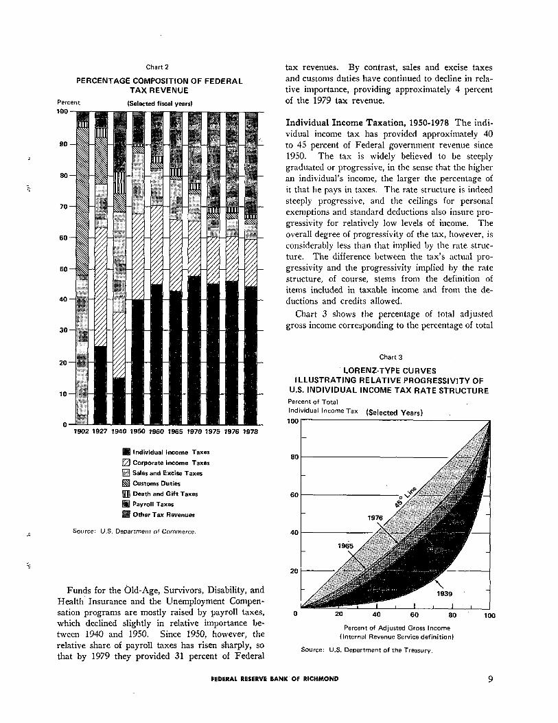
Chart 2 tax revenues. By contrast, sales and excise taxes

PERCENTAGE COMPOSITION OF FEDERAL and customs duties have continued to decline in rela-

TAX REVENUE tive importance, providing approximately 4 percent

Percent (Selected fiscal years) of the 1979 tax revenue.

1902 1927 1940 1950 1960 1965 1970 1975 1976 1978

Individual Income Taxes

Corporate Income Taxes

q Sales and Excise Taxes

q Customs Duties

Death and Gift Taxes

Payroll Taxes

Other Tax Revenues

Source: U.S. Department of Commerce.

Funds for the Old-Age, Survivors, Disability, and Health Insurance and the Unemployment Compen- sation programs are mostly raised by payroll taxes, which declined slightly in relative importance be- tween 1940 and 1950. Since 1950, however, the relative share of payroll taxes has risen sharply, so that by 1979 they provided 31 percent of Federal

Individual Income Taxation, 1950-1978 The indi- vidual income tax has provided approximately 40 to 45 percent of Federal government revenue since 1950. The tax is widely believed to be steeply graduated or progressive, in the sense that the higher an individual’s income, the larger the percentage of

it that he pays in taxes. The rate structure is indeed steeply progressive, and the ceilings for personal exemptions and standard deductions also insure pro- gressivity for relatively low levels of income. The overall degree of progressivity of the tax, however, is considerably less than that implied by the rate struc- ture. The difference between the tax’s actual pro- gressivity and the progressivity implied by the rate structure, of course, stems from the definition of items included in taxable income and from the de- ductions and credits allowed.

Chart 3 shows the percentage of total adjusted gross income corresponding to the percentage of total

Chart 3

LORENZ-TYPE CURVES ILLUSTRATING RELATIVE PROGRESSIVITY OF

U.S. INDIVIDUAL INCOME TAX RATE STRUCTURE

Percent of Total

Individual Income Tax (Selected years)

0 20 40 60 80 100

Percent of Adjusted Gross Income

(Internal Revenue Service definition)

Source: U.S. Department of the Treasury.

FEDERAL RESERVE BANK OF RICHMOND 9

individual income taxes paid by taxpayers in various income groupings for selected years. This device, called a Lorenz curve, provides an indication of the degree of disproportionality of the tax burden.

In cases where everyone pays taxes in equal pro- portion to income, the Lorenz curve coincides with the 45 degree line. By definition, the more pro- gressive the tax, the more the curve lies below the line. A curve representing a regressive tax would lie above the 45 degree line. The graphs are based on published IRS data. The published figures are classified into fewer income brackets, particularly

in the higher income categories, than is ideal for graphing the Lorenz curves. Even so, Chart 3 illustrates some of the changes in the progressivity of the individual income tax over time. It shows that the tax became considerably less progressive between 1939 and 1950, but that the largest part of the reduction in progressivity was completed by 1955. The tax was only slightly less progressive in 1976 than in 1955.

Although the Lorenz curves indicate relatively little change in the progressivity of individual income

taxes between 1965 and 1976, progressivity actually increased slightly over that span. Much of the in- crease involved a movement of the tax burden from lower income classes to the upper middle and upper income classes. Examples of the effects of these changes in progressivity between 1965 and 1976 are shown in Table I.

Progressivity changes since 1965 largely reflect the effect of increases in the standard deduction (now termed the zero-rate bracket). The standard deduction for a single return was raised in stages from 10 percent ($1000 maximum) in 1965 to 13 percent ($1500 maximum) in 1971, and finally, to 16 percent ($2400 maximum) in 1976. As a result, aggregated standard deductions (or low income

allowances) increased rapidly during the seventies, from $20 billion in 1970 to $78.5 billion in 1976. The personal exemption was also increased from $600 to $750 per person during the 1965-1976 period,

but that increase amounted to very little in constant dollar terms.

The minimum tax provision, which became effec-

tive in 1970, may also have had some impact upon the progressivity of the tax structure since 1965, although it is difficult to estimate its extent. This

provision was intended to increase taxes on selected income and deduction items that were afforded special tax treatment. The 1976 Act, effective for 1977, increased the effective tax on such tax prefer- ences nearly seven fold. These minimum tax pro- visions thus increased the taxes paid by the upper income groups, who had in the past been able to receive more of their income from less taxable (or

nontaxable) sources. Some other major changes in individual income

taxes over the 1950-1978 time period are shown in Box I. As indicated, tax credits of various kinds

lower Income Group

Year of 1976

Year of 1965

Selected Middle Income Group

Year of 1976

Year of 1965

Upper Income Group

Year of 1976

Year of 1965

Table l

INDIVIDUAL INCOME TAXES PAID BY INCOME* GROUP

Income Levels (in 1976 dollars)* *

$9000 or less

$9021 or less

Percent of Total Adjusted Gross

Income Received

16.2

17.9

Percent of Total Individual

Income Tax Bill

5.2

8.8

$20,000 to $30,000 23.4 24.4

$18,042 to $27,063 21.3 21.6

$200,000 or more 1.5 7.0

$180,423 or more 2.2 7.6

* Adjusted Gross Income as reported to the IRS.

**Based upon the Consumer Price Index for Urban Wage Earners and Clerical Workers, the price level rose 80.4 percent between 1965 and 1976. The 1965 figures are adjusted accordingly.

Source: U. S. Department of the Treasury.

10 ECONOMIC REVIEW, MAY/JUNE 1980

proliferated during the 1965-1976 period. The gen- is far more important for corporate taxes, lowered

era1 tax credit, an item that supplemented the per- personal tax revenues by $1.9 billion in 1976, where- sonal exemption until 1979 when the latter was as the childcare and the purchase of new principal

raised, reduced revenue by the largest amount in residence credits together totaled slightly over $0.5 1976, $9.3 billion. The investment tax credit, which billion.

Box I

SUMMARY OF MAJOR LEGISLATION CONCERNING INDIVIDUAL INCOME TAXES, 1950-1978

1950 Tax rates comprised a 3 percent normal rate plus a graduated surtax ranging from 17 to 88 percent. The Revenue Act of 1950 increased tax rates by eliminating a series af percentage reduc- tions in “tentative taxes” that were in effect during 1948 and 1949. This change became effective as of October 1. The net combined taxes (normal plus surcharge) were limited to 87 percent of net income, compared to 77 percent in the previous year. The withholding tax rate was 18 percent.

1951 To help finance the war in Korea marginal surtax rates were increased effective November 1, 1951 to a range of 19.2 to 89 percent, making marginal tax rates as high as 92 percent. Statu- tory reductions on the combined normal tax and surtax were eliminated, and the ceiling on com- bined taxes was raised to 89 percent of net income. Withholding tax rates were increased to 20 percent.

1954 The normal tax and surtax were combined into one rate structure. Marginal tax rates were lowered to a range of 20 to 91 percent. The level of earnings required for filing a return was raised from $600 to $1200, and the definitions of depend- ent and head of household were broadened. The retirement income credit, credits for dividends received and for partially tax-exempt interest. and the deduction for dependent childcare were intro- duced. The withholding tax rate was reduced to 18 percent.

1962 The tax credit for investment in certain de- preciable property was introduced. The rate was 7 percent of the qualified investment.

1964 The Revenue Act of 1964 lowered the tax range significantly, to 16-77 percent. It also intro- duced the income-averaging provision, and reduced withholding rates to 14 percent.

1965 The further lowering of the tax rate range to 14-70 percent, legislated in 1964. became effective in 1965.

1966 Graduated withholding was initiated. With- holding rates ranged from 14 to 30 percent.

1968 A 10 percent surcharge on income taxes was imposed, effective April 1, at a time when U. S. involvement in Vietnam was nearing its peak.

1969 The investment tax credit began to be phased out. The 10 percent surcharge was extended to cover calendar year 1969. The maximum with- holding rate was raised to 33 percent.

1970 An Additional Tax for Tax Preferences (“Minimum Tax”) of 10 percent was introduced, primarily increasing capital gains taxes. Depletion allowances were reduced, deductions for capital losses were limited, exemptions were increased, and the maximum withholding rate was reduced to 25 percent. In addition, a new minimum standard de-

duction (or low income allowance) was allowed, and the surcharge was continued at a 5 percent rate through June 30.

1971 The investment tax credit was revived. The standard deduction was increased to 13 percent ($1500 maximum). Taxes were lowered for single persons, and a maximum marginal tax of 60 percent was placed on earned income.

1972 The maximum tax rate on earned income was lowered to 50 percent.

1974 A tax rebate was approved.

1975 Primarily as temporary anti-recessionary measures, a series of tax reduction measures were adopted. The standard deduction was increased to 16 percent ($2300 maximum for a single return) and a credit of $30 per exemption was allowed. In addition, Congress approved earned income credits of up to $400 for heads of households (with depend- ents) receiving less than $8000 in adjusted gross income. Purchase-of-residence credits of up to $2000 were also approved, as was an increase in the investment tax credit from 7 to 10 percent.

1976 Some of the 1975 tax reductions were ex- tended or modified. Childcare credits (instead of the childcare deduction) were allowed. The per- sonal exemption credit became a general tax credit (the larger of $35 per exemption or 2 percent of the first $9000 of taxable income). The “Minimum Tax” was expanded through broadened definitions, reductions in deductions, and an increase in the rate to 15 percent.

1977 The general tax credit was broadened to in- clude exemptions for age or blindness. The stan- dard deduction was made independent of income, renamed the “zero bracket amount,” and incor- porated in the tax table, allowing many taxpayers to benefit.

1978 A gain of up to $100,000 on the sale of a principal residence was made tax free for persons 55 or older. The personal exemption was increased to $1000 and the zero bracket amount to $2300 for single and $3400 for married taxpayers filing joint returns. The general tax credit was repealed. The earned income-credit was increased to 10 percent of the first $5000 of income, state and local gasoline taxes were ruled nondeductible, and unemployment compensation was made taxable for single persons whose income exceeded $20,000 and married couples with incomes over $25,000. An alternative mini- mum tax, designed to insure that taxpayers with large capital gains and certain substantial itemized deductions would pay at least a basic tax, was passed (effective in 1979). Sixty percent of long- term capital gains could be deducted, however, and the basis for figuring the 50 percent maximum tax on personal service income was not to be reduced by capital gain preference items any longer.

FEDERAL RESERVE BANK OF RICHMOND 11

The earned income credit, instituted in 1976, amounted to $0.25 billion in that year. Although post-1976 data are presently unavailable because of the publication lags of IRS figures, the amount de- ducted for the earned income credit has undoubtedly increased since 1976, as more taxpayers became aware of it. It originally allowed individuals who qualified by having at least one dependent to reduce their tax payments by as much as $400 (10 percent of the first $4000 of income). Moreover, the credit was refundable in cash for individuals whose tax was less than the credit. The credit diminished rapidly as taxpayers’ incomes rose above $4000. The 1978 Revenue Act increased to $500 (10 percent on the first $5000) the maximum earned income credit and raised to $6000 the level of income at which the credit began to be phased out. The 1978 Revenue Act also allowed the general tax credit to expire and raised the personal exemption to $1000.

In conclusion, the changes in individual income

taxes since 1965 have produced a slightly more pro- gressive tax structure. This greater progressivity has been implemented mainly by changes in the tax- ation of the high and low income extremes. The changes in exemptions, the standard deduction, and the earned income credit were the principal means of reducing taxes on lower incomes. The maximum

tax rate on earned income was reduced to 50 per- cent in 1972. In spite of this change in the rate structure, higher income groups ended up paying a larger percentage of the individual income tax bill than they did in 1965.

One of the rationalizations for lowering the effec- tive tax rate on lower-income taxpayers was that lower taxes would encourage labor force participation among the unemployed (unemployment defined in the broad sense of the term). The childcare credit was specifically designed to assist working parents, but the earned income credits and the increases in the standard deduction were also expected to improve work incentives. That idea illustrates the tendency in evidence throughout the 1950-1978 time period, to use the personal income tax to promote social or economic goals that do not necessarily spring from a need to raise Federal government revenue.

Corporate Income Taxation, 1950-1978 The cor- porate income tax, as shown in Chart 2, provided 28 percent of the Federal tax revenue in 1950, but only 15 percent in 1977. About half of this decline took place between 1950 and 1965; the remainder of it occurred in the 1965-1976 period. Between 1965

and 1976, the share of revenue raised from the cor- porate income tax fell from 21 to 14 percent. The

share of taxes raised from the individual income tax, in contrast, remained relatively constant over that period.

The apparent shifting of the tax burden from cor- porations to individuals merits some discussion. One possible explanation for the shift is a relative decline in corporate income. The figures based upon the Internal Revenue Service’s (IRS) measure of cor- porate income (corporate net income), however, show no such decline. On the contrary, corporate net income rose at an average annual rate of 8.7 percent per year from 1965 to 1976, while adjusted gross income of individual taxpayers rose only 8.5 percent per year.l In contrast, corporate profits

before taxes, the measure of profits used in the Na- tional Income and Product Accounts (NIPA), rose only 6.9 percent per year between 1965 and 1976.

This latter measure of corporate profits is widely

considered to be an appropriate estimate of the state of domestic corporate business. The relatively more

rapid rate of growth of corporate net income (IRS) stems mostly from a relatively rapid growth of earn- ings in foreign branches of U. S. corporations. These foreign earnings also provide returns to owners of corporations, however, so both corporate net income and corporate profits before taxes can be interpreted as alternative measures of such returns.

The detailed differences in the two measures of corporate profit are shown in Chart 4, which reveals that the largest source of discrepancy is the treatment

of foreign revenue. To compute NIPA corporate profits, income from equities in foreign corporations is deducted from corporate net income (IRS mea- sure), and income actually received from equities in foreign corporations by all branches net of corre- sponding outflows (NIPA measure) is added back in. The difference between these two figures is quite large-$47.1 billion was deducted and $6.1 billion was added back in 1975. The major difference in the two accounts is that the smaller number does not include retained earnings of foreign branches of U. S. corporations and is measured after payment of for-

eign taxes.2 To get a measure of the before-tax

1 It might be argued! moreover, that this comparison of the tax base of individuals to that of corporations is misleading, for it compares gross revenue to net revenue. If so, adjusted gross income of individuals should be compared to corporate net income plus depreciation allowances. Using this figure, the corporate tax base rose at an average rate of 9 percent per year.

2 Because retained earnings of foreign branches do pro- vide returns to U. S. capital; however, the U. S. Depart- ment of Commerce plans to include them in NIPA corporate profits with the next benchmark revision of the data.

12 ECONOMIC REVIEW, MAY/JUNE 1980

Chart 4

DEDUCTIONS FROM AND ADDITIONS TO CORPORATE NET INCOME (IRS) NECESSARY TO

DERIVE CORPORATE PROFITS BEFORE TAXES (NIPA)

return on U. S. capital, one can adjust the NIPA Looking at the other side of the coin, if corpora-

corporate profits figure, adding back foreign taxes tions had paid U. S. taxes on their increased foreign

and retained earnings. This adjustment adds $41.0 earnings, the decline in the corporate share of the

billion to 1975 corporate profits before tax. An Federal income tax bill would have been consider- equivalent adjustment adds only $2.8 billion to 1965 ably smaller. As noted earlier, the corporate income corporate profits. Corporate profits before tax, so tax raised 14 percent of the total Federal tax bill in

adjusted, increased at an average annual rate of 7.5 1976 compared to 21 percent in 1965. Including percent per year between 1965 and 1975. ‘foreign taxes credited, however, reduces the decline

FEDERAL RESERVE BANK OF RICHMOND 13

in the corporate share by almost half. This informa- tion is shown in detail in Table II.

Foreign tax credits may be claimed by U. S. cor- porations for taxes paid by their foreign subsidiaries

to foreign governments. The amount of such tax credits claimed, only $2.6 billion in 1965, began to rise rapidly in 1974, jumping from $9.6 billion in

1973 to $20.8 billion. The credits amounted to $23.5 billion in 1976, the last year for which data are avail- able. If the foreign tax payments were included in

corporate profits taxes, the relative share of total tax revenue raised in 1976 would have been 19.5 percent rather than the 14 percent figure shown in Chart 2.

Table II

ACTUAL AND RELATIVE AMOUNTS OF CORPORATE INCOME TAX - 1965 AND 1976

(calendar years)

1965 1976

$ billions

(1)

(2)

(3)

(4)

(5)

(6)

(7)

(8)

(9)

(10)

(11)

(12)

Total Federal taxes collected $124.7

Corporation income taxes 26.0

Foreign tax credit 2.6

Extra write-off for accelerated

depreciation 7.7

Lower tax from accelerated

depreciation 3.7

Investment tax credit 1.7

Total Federal taxes plus foreign

taxes credited (line 1 plus line 3) 127.3

Line 7 plus amount taxes reduced by

accelerated depreciation 131.0

Line 8 plus investment tax credit 132.7

Corporation income taxes plus foreign

tax credit (line 2 plus line 3) 20.5

line 10 plus amount taxes lowered

through accelerated depreciation 32.2

Line 11 plus investment tax credit 33.9

$318.5

43.2

23.5

21.9

10.5

6.5

342.0

352.5

359.0

66.7

77.2

83.7

Percent

Corporate income taxes as percent of total

Federal taxes (line 2 divided by line 1) 20.8

Corporate income taxes as percent of total,

including foreign (line 10 divided by line 7) 22.4

Corporate income taxes as percent of total,

including foreign, and adjusting for

accelerated depreciation (line 11

divided by line 8) 24.6

Corporate income taxes as percent of total.

including foreign, and adjusting for

accelerated depreciation and the investment

tax credit (line 12 divided by line 9) 25.5

13.6

19.5

21.9

23.3

Source: U. S. Department of the Treasury.

Table II also shows the effects of liberalized de- preciation accounting and the investment tax credit on the corporate tax bill. If these changes had not taken place and if corporations had paid U. S. taxes

on foreign earnings, the corporate income tax would have raised 23.3 percent of the total Federal tax bill

in 1976, only slightly less than the 25.5 percent that would have been raised in 1965.

Thus, the reduction in the relative share of cor- porate taxes stem from a number of factors. Cor- porate profits and taxes, including profits and taxes in foreign countries, grew rapidly. Profits from do-

mestic operations grew less rapidly and taxes still less rapidly, due to allowances for accelerated de- preciation and the investment tax credit.

The foregoing findings about the decline in the relative share of taxes raised from corporate taxes may appear to be at odds with the oft-repeated as- sertion that corporate tax burdens have become in- creasingly onerous since the midsixties, but there is

really little conflict between the two. The findings of Feldstein and Summers [1] illustrate this point. Feldstein and Summers show that if the tax rate

on returns to nonfinancial corporate capital were measured properly, it would have been 52.5 percent

in 1965 and 64.9 percent in 1976.3 Feldstein and Summers begin their analysis using

corporate profits (NIPA) with inventory valuation

adjustments (IVA) and capital consumption allow- ances (CCA).4 To find total tax paid on the total return to capital, they first add corporate interest pay- ments to corporate profits before tax with IVA and CCA. This sum, which they term corporate source income, provides them with a measure of corporate income available to shareholders and creditors. To estimate total taxes collected on corporate source in- come, they add individual income taxes paid on divi- dends, interest, and realized capital gains-and poten-

3 This rate fluctuates widely. It was calculated to be 70 percent in 1973 and 95 percent in 1974.

4 The inventory valuation adjustment removes “inventory profits,” which arise in an inflationary environment when- ever inventories are valued at historical rather than re- placement cost. The capital consumption adjustment adjusts depreciation allowances to a consistent (straight- line) accounting method, with the depreciated item valued at replacement rather than historical cost. Econ- omists generally believe that corporate profits with IVA and CCA is a better measure of real profit than is the unadjusted figure. They come to this conclusion because “inventory profits” earned by a normal operating business enterprise must be spent immediately in re- placing the old inventory, so the gain is illusory. The capital consumption allowance is considered to be a proper adjustment for normal business enterprises be- cause firms will eventually need to replace their invest- ment so they should be allowed to deduct the entire replacement expense from their profits.

14 ECONOMIC REVIEW, MAY/JUNE 1980

tial taxes accrued yearly on unrealized gains-to corporate profits taxes. Their results, which are are shown in Table III, indicate that corporate source income has often been subject to very high rates of taxation, the highest being 95 percent in 1974. At that time, a high rate of inflation coupled with the then-extensive use of first-in-first-out (FIFO) in- ventory valuation methods to produce a large differ- ence between taxable and economic profits.

In using the NIPA definition of corporate profits,

however, Feldstein and Summers ignore a large source of corporate revenue, namely foreign oper-

ations. Table III also includes a row in which

the Feldstein and Summers figures are adjusted to include income from foreign equities and foreign

taxes.6 These adjustments recognize that foreign

income provides a return to domestic capital. Inclu-

5 Adding the income from foreign equities and the foreign tax credit to the Feldstein and Summers figures is not strictly correct, because their estimates relate only to nonfinancial corporations and the foreign numbers relate to all cornorations. but data were not available on the relative amounts of income and tax credits of the foreign sector received (claimed) by financial and nonfinancial corporations.

sion of the expanded foreign sector can make a sub- stantial difference. Most dramatically, the tax rate in 1974 is lowered from 95 to 82.4 percent.6

In summary, the tax burden placed upon returns to corporate capital can, indeed, be quite onerous and much of the burden is attributable to the corporate income tax. Critics have argued for decades that corporations are treated unfairly in that their stock- holders are subjected to “double taxation.” The im- plication of this argument, that corporate enterprise is taxed relatively more heavily than unincorporated enterprise, however, is quite debatable.

Corporations enjoy certain advantages that may outweigh the burden of “double taxation.” The other side of the “double taxation” coin is that cor-

6 While not relevant to these figures because Feldstein and Summers examine only nonfinancial corporations, the treatment of income and taxes on income from Federal Reserve Banks can also cause difficulties in interpreting the NIPA corporate profits data. The National Income and Products Accounts treats earnings of these institu- tions as part of corporate profits, but treats most of it as being taxed away as corporate profits tax. Since the Federal Reserve Banks return rather large percentages of their earnings to the Treasury, their tax rate is of course much larger than that of other corporations.

Table III

THE EFFECTIVE TAX RATE ON CAPITAL INCOME OF THE NONFINANCIAL CORPORATE SECTOR

1965 1966 1967 1968 1969 1970 1971 1972 1973 1974 1975 1976

Total Real Income 70.9 76.2 73.8

Corporate Income Tax

Taxes on Shareholders and Creditors

Dividends

Real Retained, Earnings

Nominal Capital Appreciation (accrued capital gains taxes)

Interest Income

Total Taxes

Foreign Income and Tax Credit

Tax Credits Claimed for Foreign Taxes Paid

Income on Equities in Foreign Corporations and Branches*

38.3 38.7 37.5

7.1 6.9 7.4 7.6 8.0 9.0 7.9 7.2 7.7 10.0 8.4 7.4

2.7 2.8 2.8 2.8 2.8 1.2 1.1 1.4 2.1 2.1 1.7 1.4

0.7 1.2 1.3 2.0

3.8 4.3 5.2 5.6

52.5 53.9 54.2 60.8

2.6 2.9 3.2 3.7 4.0 4.5 5.7 6.3 9.6 20.8 20.0 23.5

2.8 3.8 4.4

Total Tax (including foreign taxes) 54.0 55.0 55.2

78.7

42.7

Billions of Dollars

74.9 64.2 73.7 88.0

Percent of Total Real Income

44.5 42.5 40.5 38.0

90.2

43.9

3.0 3.5 2.1 1.8 5.0

7.7 11.7 10.7 9.6 11.3

66.0 67.8 62.3 58.0 70.0

Billions of Dollars

5.0 5.2 6.0 7.6 9.2 15.6

Percent of Total Income (including foreign)

61.6 66.7 68.2 63.5 59.0 68.8

* Portion not otherwise included in corporate profits before taxes.

Sources: Feldstein and Summers [1] and U. S. Department of Commerce.

FEDERAL RESERVE BANK OF RICHMOND

76.2 100.2 126.3

56.0 40.8 42.5

9.4 4.8 2.9

17.2 13.6 10.7

94.9 69.3 64.9

36.8 41.0 n.a.

82.4 63.3 n.a.

15

porations may retain earnings, thus allowing share- holders to defer taxes on these earnings until they sell their shares-at which time the increase in the value of the shares is treated as a capital gain. Cor- porations also enjoy certain advantages in setting up pension plans, as well as the widely-known legal advantages of limited liability (which is less of an advantage nowadays than it once was, for limited liability can be conferred to “limited partners”) and immortality. Advantages such as these may partially account for the continued rapid growth of the cor- porate form of business relative to the noncorporate

form.

The three sets of data available that allow com- parisons of corporate and noncorporate growth are total receipts, number of firms organized, and income originating by form of organization. Total receipts

of corporations increased at a 10.6 percent average

annual rate between 1965 and 1976 while receipts of partnerships and proprietorships increased at only a 6.3 percent rate. Between 1973 and 1976, corporate receipts increased at a 12 percent average annual rate compared to 7 percent for noncorporate receipts.

will provide an estimated 32 percent of all Federal tax

revenue. Most of these payroll taxes are used to finance the Old-Age, Survivors, Disability, and Health Insurance (the so-called “social security” system). These taxes are thus tied to certain benefit payments. The payroll tax schedules are therefore designed to allow the various social security trust funds to meet their projected benefit needs. As a result, payroll tax revenue increased from $19 billion in 1965 to $123 billion in 1978 (an average annual rate of increase of 15.4 percent, while other Federal taxes were increasing at an average rate of 8.7 per- cent). The payroll tax revenue is estimated to be $161.5 billion in 1980, thus registering a 14.6 percent annual growth rate from 1978.

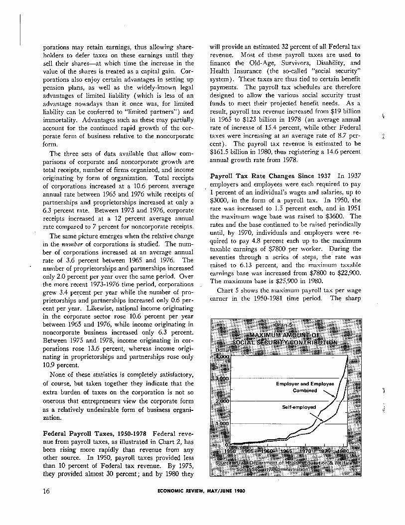
Payroll Tax Rate Changes Since 1937 In 1937 employers and employees were each required to pay 1 percent of an individual’s wages and salaries, up to $3000, in the form of a payroll tax. In 1950, the rate was increased to 1.5 percent each, and in 1951 the maximum wage base was raised to $3600. The rates and the base continued to be raised periodically until, by 1970, individuals and employers were re-

quired to pay 4.8 percent each up to the maximum taxable earnings of $7800 per worker. During the seventies through a series of steps, the rate was raised to 6.13 percent, and the maximum taxable earnings base was increased from $7800 to $22,900. The maximum base is $25,900 in 1980.

Chart 5 shows the maximum payroll tax per wage earner in the 1950-1981 time period. The sharp

16 ECONOMIC REVIEW, MAY/JUNE 1980

The same picture emerges when the relative change in the number of corporations is studied. The num- ber of corporations increased at an average annual rate of 3.6 percent between 1965 and 1976. The number of proprietorships. and partnerships increased only 2.0 percent per year over the same period. Over the more recent 1973-1976 time period, corporations grew 3.4 percent per year while the number of pro- prietorships and partnerships increased only 0.6 per- cent per year. Likewise, national income originating in the corporate sector rose 10.6 percent per year between 1965 and 1976, while income originating in noncorporate business increased only 6.3 percent. Between 1975 and 1978, income originating in cor- porations rose 13.6 percent, whereas income origi- nating in proprietorships and partnerships rose only

10.9 percent.

None of these statistics is completely satisfactory,

of course, but taken together they indicate that the

extra burden of taxes on the corporation is not so

onerous that entrepreneurs view the corporate form

as a relatively undesirable form of business organi- zation.

Federal Payroll Taxes, 1950-1978 Federal reve- nue from payroll taxes, as illustrated in Chart 2, has been rising more rapidly than revenue from any other source. In 1950, payroll taxes provided less than 10 percent of Federal tax revenue. By 1975,

they provided almost 30 percent; and by 1980 they

increases in recent years illustrate vividly the in- creasing relative burden of the payroll taxes on middle and upper income groups (the data are shown in nominal terms; converted into constant dollars the

burden would appear to be lower). These increases have unfortunately coincided with the worst decade of stagflation in American experience. The burden of paying for social security benefits, of course, in- creases during stagflation, which partly explains the sharp increases in payroll taxes over the past decade. In addition, many economists would argue that pay- roll taxes contribute more to stagflation than other types of taxes (see discussion below).

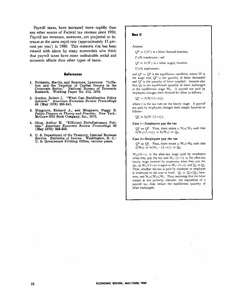
A Digression on Economic Effects of Payroll Taxes The rapid increases in payroll taxes have been viewed with alarm by many economists, who fear their possible adverse effects on the accumulation of capital and on the wage and price structure of the economy. Theoretically, in a competitive economy the wage earner bears the burden of the payroll tax and it makes no difference whether the tax is nom- inally levied on the employer or the employee. This argument is illustrated algebraically in Box II.’ As this exhibit shows, the tax reduces the quantity of

labor demanded and supplied by the same amount regardless of whether it is the “employer’s share” or the “employee’s share.” In this example, the wage earner, who receives the eventual benefits of the OASDHI system, pays the tax.

The argument in Box II, however, depends cru- cially upon the assumption of competition in product and labor markets. As Richard and Peggy Musgrave argue in Public Finance in Theory and Practice [3], however, market power allows wage earners to pass along the burden of a payroll tax to the general public. They also argue that, in reality, it can make a difference if the tax is paid by the employer rather than the employee,

In particular, the Musgraves state that:

If payroll taxes are increased, unions may accept an increase in the employer contribution without demanding a wage increase, but they will hardly agree to a reduction in their wage rate in order to offset an increase in the employer contribution. Firms, in turn, will not absorb the increase in their contribution in reduced profits, but will make it an occasion to raise prices. [3, pp. 392-393].

Wage earners will, therefore, not bear the entire burden of the tax, for through the price effect, the tax lowers real incomes generally. The Musgraves conclude that the price effect will be particularly strong when increases in payroll taxes are designated to be paid by employers rather than employees. Thus, in a noncompetitive world, actions designed to in-

crease the payroll tax can have an inflationary impact

upon the economy, and the inflationary effect can be larger if the tax increase is stipulated to come from the “employer’s share.”

This conception of the effects of the payroll tax is a source of the argument that increases in payroll taxes promote inflation. Arthur Okun [4, p. 351] and Robert Gordon [2, p. 339], among other influ- ential economists, argue that a reduction in payroll taxes can be useful in coping with stagflation. Gordon also points out that

the prospective increases in payroll taxes in the late 1970’s and early 1980’s amount to a series of

‘mini supply shocks.’ A monetary authority ad- hering to a [constant growth rate rule for the money supply] would find that these cost increases would increase unemployment. An accommodative money supply would shift the burden of the [tax] . . . from unemployment to real income losses for those holding assets yielding nominal-fixed returns [2, p. 338].

Summary Federal taxes have risen precipitously in the U. S. during the past half century. Between 1930 and 1950, Federal tax receipts rose from ap- proximately 3.2 percent of GNP to 17.5 percent. Since 1950, the share of GNP going to Federal taxes has leveled off at around 20 percent.

The method of raising Federal tax revenues has also changed dramatically. In 1927, individual in- come taxes provided approximately 25 percent of Federal tax revenues; corporate income taxes ap- proximately 37 percent; sales and excises, 12 per- cent; customs duties, 19 percent; and payroll taxes, 5 percent. By 1950, individual income tax receipts were a greatly enlarged 40 percent of all Federal tax receipts; corporation income taxes, 32 percent; sales and excises, 20 percent; customs duties, 3 percent; and payroll taxes, 9 percent. By 1977, individual income taxes provided 45 percent of total Federal revenue; payroll taxes, 29 percent; corporate income taxes, 15 percent; and sales and excises, 8 percent.

The major changes in taxation since 1950, there- fore, have been the relative decline in the corporate income tax and the rise of the payroll tax. The decline

in the share of the corporate income tax is somewhat illusory because of the tax treatment of foreign earn- ings and the foreign tax credit. The implication that one might draw from the reduction in the share of tax revenues raised from corporate income taxes, however, that the corporate tax burden is less oner- ous than in earlier years, is also illusory. The

effective tax rate on corporate capital, according to the calculations of Feldstein and Summers, in- creased considerably between the late sixties and early seventies, primarily because of inflation.

FEDERAL RESERVE BANK OF RICHMOND 17

Payroll taxes, have increased more rapidly than any other source of Federal tax revenue since 1950. Payroll tax revenues, moreover, are projected to in- crease at the same rapid rate (approximately 15 per-

cent per year) in 1980. This meteoric rise has been viewed with alarm by many economists who think that payroll taxes have more undesirable social and economic effects than other types of taxes.

References

1. Feldstein, Martin, and Summers, Lawrence. “Infla- tion and the Taxation of Capital Income in the Corporate Sector.” National Bureau of Economic Research. Working Paper No. 312, 1979.

2. Gordon, Robert J. “What Can Stabilization Policy Achieve.” American Economic Review Proceedings 68 (May 1978) 336-341.

3. Musgrave, Richard A., and Musgrave, Peggy B. Public Finance in Theory and Practice. New York: McGraw-Hill Book Company, Inc., 1973.

4. Okun, Arthur M. “Efficient Disinflationary Poli- cies.” American Economic Review Proceedings 68 (May 1978) 348-362.

6. U. S. Department of the Treasury, Internal Revenue Service. Statistics of Income. Washington, D. C.: U. S. Government Printing Office, various years.

Box II

Assume

= f(W) is a labor demand function,

f'<0, continuous; and

= h(W) is a labor supply function,

h'>0, continuous;

and is the equilibrium condition, where W is the wage rate. is the quantity. of labor demanded and is the quantity of labor supplied. Assume also that is the equilibrium quantity of labor exchanged at the equilibrium wage W0. A payroll tax paid by employers changes their demand for labor as follows :

= f(W/(l-t)),

where t is the tax rate on the hourly wage. A payroll tax paid by employees changes their supply function as follows:

= h(W•(l-t)).

Case l-Employers pay the tax

Thus, there exists a W1<W0 such that f(W1/(1-t)) = h(W1) =

Case 2-Employees pay the tax

Thus, there exists a W2>W0 such that

f(W2) = h(W2 • (l-t)) =

W1/(l-t) is the after-tax wage paid by employers when they pay the tax and W2•(l-t) is the after-tax hourly wage received by employees when they pay the tax, so W1/(l-t) is equal to W2•(l-t) and Thus, whether the tax is paid by employer or employee is irrelevant to the case at hand. how- ever, and W1<W0<W2. Thus, assuming that the labor supply is not perfectly inelastic, the imposition of a payroll tax does reduce the equilibrium quantity of

labor exchanged.

18 ECONOMIC REVIEW, MAY/JUNE 1980

DENNIS H. ROBERTSON AND THE

MONETARY APPROACH TO EXCHANGE RATES

Thomas M. Humphrey

Prominent among competing explanations of ex- change rate determination in a regime of floating exchange rates is the so-called monetary approach, which holds that the exchange rate between two na- tional currencies is determined by current and pro- spective relative supplies of and demands for those national money stocks. This theory has a long tradi-

tion going back more than 300 years. As an integral part of pre-Keynesian international monetary theory, it formed the central analytical core of classical and neoclassical explanations of exchange rate behavior. Although it was temporarily eclipsed by the rival elasticities and foreign trade multiplier or income- expenditure approaches that gained popularity with the domination of the Keynesian revolution, it has recently made a comeback and today is widely em- ployed by academic and business economists to ex- plain the behavior of exchange rates in the post-

Bretton Woods era of generalized floating. For example, such well-known economists as Robert Barro, John Bilson, Jacob Frenkel, and Michael Mussa have successfully employed the monetary ap- proach to account for recent exchange rate experi- ence, as have analysts at Citibank, Chase Manhattan, and other financial institutions. Finally, it is worth noting that certain segments of the financial press, notably the editorial pages of the Wall Street Journal, regularly espouse the monetary approach.

Corresponding to the growing popularity of the monetary approach has been an accompanying inter- est in its historical antecedents. Accordingly, in the past few years Jacob Frenkel, Johan Myhrman, and Mordechai Kreinin and Lawrence Officer, respec- tively, have published papers dealing with the doc- trinal development of that approach.1 These papers, however, suffer from one serious omission. For while they cite several prominent economists writing in the 1920s-notably Cassel, Gregory, Hawtrey, and Keynes-as important early proponents of the mone- tary approach, they say nothing about the great Brit- ish economist Dennis Robertson. The result is to

1 See Frenkel [2], Myhrman [12], and Kreinin and Officer [7, pp. 28-31].

foster the erroneous impression that Robertson, gen- erally recognized as one of the leading monetary theorists of the 20th century, had virtually nothing to say about the monetary approach when in fact he was one of its principal proponents. Not only did he

endorse and utilize the established components of the monetary approach, he also presaged recent develop- ments in the theory of exchange rate expectations. For these reasons his work merits consideration.

The purpose of this article is twofold. First, it identifies and explains the essentials of the monetary approach to exchange rates. Second, it documents Robertson’s views on that approach. This is a fairly easy task, since the bulk of Robertson’s work on float- ing exchange rates is contained in one volume, namely the 1929 edition of his famous Cambridge Economic Handbook Money.2 In that book he divides his discussion of exchange rate determination into two sections, one dealing with conditions of monetary stability and the other dealing with episodes of violent and rapid inflation. His views on the

monetary approach are to be found in these two sections. What particular elements identifying the

monetary approach should one look for in his views ?

Basic Ingredients of the Monetary Approach To

demonstrate that Robertson was a proponent of the monetary approach, it is necessary to spell out the key ingredients or propositions that characterize that approach.3 These elements include the following :

1. MONETARY VIEW OF LONG-RUN EX- CHANGE RATE DETERMINATION. The mone- tary approach holds that the long-run equilibrium exchange rate between two national currencies is determined chiefly by relative national money supplies and demands operating through relative national price levels. This proposition implies a particular monetary transmission mechanism or channel of causation linking money to exchange

2 Unless otherwise noted, all references are to the 1963 reprint of the 1947 edition, which is virtually the same as the 1929 edition as far as the discussion of floating ex- change rates is concerned.

3 The essentials of the modern monetary approach are expounded more fully in Bilson [1], Frenkel [2], Frenkel and Clements [3], and Mussa [9, 10].

FEDERAL RESERVE BANK OF RICHMOND 19

rates. Accordingly, the monetary approach speci- fies such a mechanism and identifies quantity theory of money and purchasing power parity rela- tionships as the key links in that mechanism. The quantity theory says that the general price level is determined by the demand-adjusted money stock, i.e., by the nominal quantity of money per unit of real money demand. In other words, the price level equates money supply and demand by de- flating the real value of the nominal money stock to the level people desire to hold. By contrast, the purchasing power parity doctrine states that the long-run equilibrium exchange rate tends to equal the ratio of the price levels in the two countries concerned. This condition ensures that the real (exchange rate-adjusted) price of goods is every- where the same so that there exists no arbitrage advantage to buying in one country over the other. It also ensures that both moneys have the same real (exchange rate-adjusted) purchasing power such that there exists no incentive to switch from one currency to the other. Taken together, the quantity theory and purchasing power parity components imply that relative money sup- plies and demands operating through relative na- tional price levels determine the long-run equilib- rium exchange rate. And according to the mone- tary approach, the stability of that-equilibrium is ensured by the self-correcting characteristic of the purchasing power parity mechanism itself. Thus, should random deviations from purchasing power parity occur, they would be quickly eliminated. For by overvaluing one currency and undervaluing the other on the foreign exchanges, such deviations would shift demand from the former currency to the latter and in so doing bid the exchange rate back to purchasing power parity equilibrium.

2. ASSET MARKET VIEW OF SHORT-RUN EXCHANGE RATE BEHAVIOR. The foregoing proposition refers to exchange rate determination in the long run when purchasing power parity holds. With respect to exchange rate determination in the short run when purchasing power parity may not hold, the monetary approach advances the so-called asset market view. According to that view the exchange rate between two national currencies behaves like an asset price in an efficient market, adjusting instantly to a level at which both asset (i.e., money) stocks are willingly held. As an effi- cient asset price, the current spot exchange rate is particularly sensitive to expectations of future ex- change rates, expectations that are heavily con- ditioned by recent and current monetary policy and other indicators of the future course of-monetary policy. More generally, as an efficient asset price the current exchange rate embodies all available information about current and prospective events likely to affect the future external values of the two currencies and adjusts instantaneously to in- corporate new information about changed condi- tions. In this manner new information about future exchange rates is discounted into the current exchange rate analogously to the way that news about the future profitability of a corporation is discounted into the current market price of its equity shares.

3. ROLE OF EXPECTATIONS. As noted above, one implication of the asset market view is that the current spot exchange rate is strongly influ- enced by current expectations of future exchange rates. This is so because the expected rate of change of the exchange rate is the same as the anticipated rate of return from holding foreign rather than domestic money. As such, expectations affect the relative demand for the two currencies and thereby influence the exchange rate. Thus a rise in the expected rate of depreciation of the exchange rate will, by raising the expected yield from holding foreign rather than domestic cur-

rency, shift demand from the latter to the former thereby depreciating the current spot exchange rate. In short, the spot exchange rate is deter- mined by exchange rate expectations operating through relative money demands.

4. RATIONAL EXPECTATIONS HYPOTHESIS. Besides explaining how expectations affect ex- change rates, the monetary approach also explains how expectations themselves are determined. Ac- cording to the monetary approach, people formu- late exchange rate expectations consistent with the way that exchange rates are actually deter- mined in the economy. Thus. if actual observed exchange rates are determined by money supply and demand, it follows that expected future ex- change rates are determined by forecasts of future values of those same monetary variables. In par- ticular, the monetary approach maintains that exchange rate expectations are governed by expec- tations of future money supplies per unit of real money demands. These latter expectations, the monetary approach asserts, are formed from all available information about prospective events likely to influence future money supplies and de-

mands. In so arguing, the monetary approach advances the rational expectations hypothesis ac- cording to which the market’s aredictions of future exchange rates are the same as those generated by the actual mechanism that determines exchange rates. This assumption ensures that the monetary approach is internally consistent, i.e., that its explanation of expectations formation is consistent with its explanation of exchange rate determina- tion. Such consistency is thought to be character- istic of the forecasting behavior of rational agents who use knowledge of the actual exchange rate- generating mechanism in formulating expectations of future exchange rates. Knowing that money supplies and demands determine actual exchange rates, rational agents will predict future exchange rates from forecasts of future money supplies and demands.

Constituting the central analytical core of the modern

monetary approach to floating exchange rates, the

foregoing ingredients must be found in Robertson’s

work if he is to be judged a proponent of that ap-

proach. Accordingly, the following paragraphs show

what he had to say on each of the propositions listed

above.

Before discussing Robertson’s views, however, it

should be pointed out that the long-run quantity

theory version of the monetary approach (i.e., propo-

sition one above) long predates him. That version

dates back at least to the mid-sixteenth century when

Spanish scholastic writers of the Salamanca School

used it to explain fluctuations in the Spanish currency

price of Flemish money.4 And in the famous Bank

Restriction Controversy of the early 1800s, David

Ricardo, John Wheatley, and other bullionist writers

employed it to explain the fall of the paper pound on

the foreign exchanges following Britain’s switch from

fixed to floating exchange rates during the, Napole-

onic wars.5 The theory was endorsed by A. Marshall

4 See Grice-Hutchinson [6, p. 5.51].

5 See Myhrman [12, pp. 170-173].

20 ECONOMIC REVIEW, MAY/JUNE 1980

in the late 1880s and revived by Gustav Cassel in 1916 to explain exchange rate movements during World War I.6 After the war the theory was widely used to explain the fall of the German mark in the famous hyperinflation episode of the early 1920s.7 Robertson of course was well aware of this and goes out of his way to disclaim any originality in his pre-

sentation of the theory. His views on this long estab- lished or “customary” (as he called it) doctrine are presented immediately below [14, p. 58].

Long-Run Equilibrium Exchange Rate The first proposition of the monetary approach states that the long-run equilibrium exchange rate between two na- tional currencies. is determined by the relative sup- plies of and demands for those national money stocks. That Robertson was in basic agreement with this proposition is evident from his discussion of the de-

termination of the “normal level of the rate of ex- change” between two inconvertible paper currencies

( or “arbitrary independent standards” as he called them) [14, pp. 57, 58]. In his discussion he attrib- utes the state of the exchanges largely to the under- lying monetary conditions in the two countries con- cerned. Although he denies that these monetary factors are the sole determinants of exchange rates, he repeatedly refers to them as the dominant deter- minants. For example, in various places he specific- ally identifies “the monetary situation” or “the supply of money in the two countries” or “the state of a country’s monetary glands” as “the essential condi- tion for the maintenance of a given rate of exchange” [14, pp. 60, 103]. Elsewhere, when discussing the stability of exchange rate equilibrium, he reiterates his belief in the importance of the monetary factor when he notes that the exchange rate must always gravitate to that particular equilibrium level “which the existing money supply of the country as com- pared with that of other countries renders perma- nently maintainable” [14, p. 101].

Embodied in the monetary approach is a particular model of the monetary transmission mechanism con- necting money with exchange rates. As usually pre- sented, that model contains quantity theory of money and purchasing power parity relationships, the former linking money supplies and demands to prices and the latter linking prices to the exchange rate. These same elements can be found in Robertson’s work. Consistent with the monetary approach, he

6 On Marshall, see Eshag [5, pp. 26-34]. On Cassel, see Myhrman [12, pp. 177-178].

7 See Ellis [4, pp. 209-236].

combines them to arrive at the conclusion that ex- change rates are determined largely by relative money supplies and demands operating through price levels, particularly the prices of internationally-traded goods. He reaches this conclusion via the following route.

First, he argues that “the value of money . . . depends on the conditions of demand for it and the quantity of it available” [14, p. 32]. This of course is the quantity theory of money which may be written as

(1) P = M/D

where P is the general price level (the inverse of the value of money), M the nominal money stock, and D the real demand for money. This equation, which says that the price level is determined by and varies equiproportionally with the stock of money per unit of real money demand, is expressed by Robertson in the following words: “given the conditions of de- mand for money . . . the general level of prices varies directly as the quantity of money available” [14, p. 26]. Note that equation 1, which may be written

as M/P = D, also says that the price level adjusts to equate the real (price-deflated) value of the nomi- nal money stock with the public’s real demand for it, thereby clearing the market for real cash balances. Consistent with his adherence to the quantity theory, Robertson employs this, alternative interpretation when he declares that, given the public’s real demand for money, a ten percent rise in the nominal money stock will produce a corresponding ten percent rise in the price level such that the price-deflated or “aggregate real value of the public’s money supply is no greater than it was before” [14, p. 76].

Second, he presents the purchasing power parity relationship, stating that “the normal level of the rate of exchange depends on the relative price levels, in

the moneys of the two countries, of the things which enter into trade between them” [14, p. 58]. This of course is the traded-goods or commodity arbitrage version of purchasing power parity, which holds that the equilibrium exchange rate is equal to the ratio of the domestic and foreign price levels of interna- tionally traded goods. In symbols

(2) E = PT/PT *

where E is the exchange rate (defined as the do- mestic currency price of a unit of foreign currency), and PT and PT * are the domestic- and foreign cur- rency prices of traded goods, respectively.

Third, he assumes that in long-run equilibrium the price of traded goods bears a certain equilibrium

FEDERAL RESERVE BANK OF RICHMOND 21

relationship to the general price level. This relation- ship can be expressed as

(3) PT = RP

where R denotes the equilibrium ratio of traded- goods prices to general prices in the home country, as can be seen by rewriting the equation in the form R = PT/P. Representing the relative price of traded goods in terms of the general price level, this equa-

tion summarizes the equilibrium structure of prices in the home country. This notion of a stable equilib- rium price structure can be inferred from Robert- son’s statement that he is assuming conditions of “comparative stability” characterized by the absence

of “violent and continuous monetary dislocation” [14, p. 58]. It can also be inferred from his willingness to substitute traded-goods prices interchangeably for general prices as a measure of the value of money.*

Fourth, he substitutes equations 1 and 3 into equa- tion 2 to obtain the following result

(4) E = (1/PT)R M D *

which says that given foreign prices and the domestic

price structure the exchange rate depends on the domestic money supply per unit of real money de- mand. Robertson states this result when he declares that “given the price level of traded goods in terms of utopes [Robertson’s hypothetical foreign currency]

. . . the monetary situation in England turns out to be the essential condition for the maintenance of a given rate of exchange” [14, p. 60].

Finally, he assumes that prices in the foreign coun- try are determined analogously to their domestic counterparts. Specifically, the foreign price of traded goods is linked through a price structure variable to the foreign general price level which is determined by foreign money supply and demand. Substituting this

assumption into equation 4 yields the following ex- pression

R D* M (5) E = R* D M*

which says that the long-run equilibrium exchange

rate is determined by the product of three groups of factors, namely relative price structures, relative real money demands, and relative nominal money sup- plies, respectively. Of these three groups, the first 9

8 See Robertson [14, p. 61] where he refers to the value of money measured “in terms of traded goods.”

9 Asterisks refer to foreign country variables.

two capture the effect of real (nonmonetary) influ- ences on the exchange rate while the third captures purely monetary influences.

Equation 5, which summarizes Robertson’s theory

of long-run exchange rate determination, puts him squarely in the ranks of the monetary approach. To be sure, the equation does contain a relative price structure variable (and hence an extra channel through which real factors can affect exchange rates)

not usually found in the monetary approach’, Apart from this, however, the equation is exactly the same as that advanced by the monetary approach. It em- bodies the latter’s assumption of quantity theory and purchasing power parity linkages running from money to the exchange rate, and therefore, in Robert- son’s words, “serves to remind us that the exchange rates are . . . connected with the supply of money in the two countries” [14, p. 60]. Moreover, like the monetary approach, it identifies relative money de- mands and supplies as key determinants of the ex-

change rate. Finally, it yields the standard mone- tarist homogeneity postulate that a ceteris paribus rise in the relative money supply produces an equi- proportional rise in the nominal exchange rate. That Robertson accepts this homogeneity postulate is evi- dent from his statement that if “the supply of Utopian money had become double . . . while neither the

supply of English money nor any other conditions of

the problem had changed, we should not be surprised

to learn that the rate of exchange had become 10

utopes to the pound instead of 5” [14, p. 60]. In

short, to the extent he accepts these features, Robert-

son is a proponent of the monetary approach.

Before concluding this section it is necessary to compare Robertson’s views of the purchasing power parity relationship with those of the monetary ap- proach. Regarding purchasing power parity there are at least three main issues, the first referring to the

relevant price levels to use in calculating the parity. On this issue Robertson disagrees with the monetary approach. For whereas the latter holds that general prices should be employed in computing the pur- chasing power parity, Robertson argues that only the prices of internationally traded goods should be used. Thus in stating that the equilibrium exchange rate tends to equal the ratio of domestic to foreign prices, he makes it emphatically clear that he is referring to the prices of “traded goods” or “those goods which are the subject of trade” [14, pp. 60-61]. He ap- parently believes that purchasing power parity logi- cally holds only for prices subject to international equalization by commodity arbitrage, for he states that it is only the movement of such prices “which

22 ECONOMIC REVIEW, MAY/JUNE 1980

we should expect to correspond closely to the move- ments of the exchanges” [13, p. 141]. Not men- tioned by him is a point stressed by the monetary approach, namely that, with intercommodity substi- tution in production and consumption and inter- industry competition for factors of production, the prices of traded and nontraded goods tend to be sufficiently closely related such that general prices can be used to approximate the purchasing power parity. Nevertheless, on at least one occasion he apparently accepts this proposition. For he uses a

general price index to proxy the purchasing power parity claiming that, as a practical matter, the index is “good enough . . . to illustrate the general normaI relation between price levels and exchanges” [13, p. 141].

The second issue relating to purchasing power

parity concerns the purpose or role of the exchange

rate. On this issue the monetary approach contends

that the chief function of the exchange rate is to clear

the market for money balances by equating the real

purchasing power of both currencies such that both

money stocks are willingly held. That Robertson is

in substantial agreement with this point can be in-

ferred from such comments of his as “the normal rate of exchange between [two countries] depends on the relative values of their moneys in terms of traded goods,” and “the normal rate . . . reflects the condi- tion of the country’s money supply as compared with that of the other countries” [14, pp. 61, 102]. The first comment implies that the purchasing power parity exchange rate embodies the relative price de- flator that, when applied to relative nominal na- tional money supplies, serves to equalize the real

(price-deflated) value of money across nations. Robertson’s second comment implies that exchange rates, like prices, also summarize the underlying monetary conditions in each country. Both implica- tions are consistent with the notion that the ex- change rate functions to clear the market for national money balances by equating the real purchasing power of both currencies such that there exists no incentive to switch from one currency to the other.

Robertson recognizes, as do proponents of the monetary approach, that the exchange rate also plays a commodity arbitrage role, adjusting to equalize the real price of traded goods across nations so that there exists no advantage to buying in one market over another. In this connection he points out that if the real price of goods were to differ between countries such that it became advantageous to buy in the cheaper country and sell in the dearer one, the re- sulting excess demand for the currency of the former

country would quickly bid the exchange rate up to the purchasing power parity level at which the com- mon currency prices of goods are everywhere the same. While recognizing the arbitrage function of the exchange rate, however, he nevertheless appar- ently places greater emphasis on its money market clearing role. For whereas he mentions the com- modity arbitrage role but once, he repeatedly contends that the equilibrium exchange rate must be consistent with the underlying monetary conditions in the coun- tries concerned [14, pp. 59, 60, 61, 101, 103]. In so doing, he implicitly endorses the proposition that the chief function of the exchange rate is to achieve international monetary equilibrium by clearing the markets for national money balances.

As for the third issue, namely whether the pur- chasing power parity is an equilibrium condition or a

cause-and-effect relationship between prices and ex- change rate, Robertson obviously holds it to be the former. In so doing, he agrees with the monetary

approach. Like proponents of that approach, he

maintains that prices and the exchange rate are both endogenous variables simultaneously determined by underlying monetary conditions. As he puts it, both variables are “rendered possible by the monetary situation,” i.e., both are established at levels “which the existing money supply of the country, as com- pared with that of other countries, renders perma- nently maintainable” [14, pp. 60, 101]. In short, on this issue as with most of the others, Robertson ad- heres to the monetary approach.

Asset Market View The second component of the monetary approach is the asset market view ac- cording to which the exchange rate behaves like an efficient asset price, embodying all available informa- tion about the future values of the currencies and adjusting instantaneously to incorporate new infor- mation about changed circumstances. Robertson possessed a sophisticated understanding of the asset market view, which he used in explaining “the mis- behavior of the foreign exchanges” during the post- World War I hyperinflation episodes of the early 1920s. For example, regarding the proposition that the current exchange rate registers the market’s per- ceptions about the future exchange rate-i.e., market participants discount the expected future value of the currencies into the current spot exchange rate-he says that exchange rates tend “to reflect the degree of confidence felt in the future of a country’s money by the nimble-witted dealers in exchange” [14, p. 101]. These dealers he describes as being especially “well-informed and impressionable” implying that, consistent with the concept of an efficient market,

FEDERAL RESERVE BANK OF RICHMOND 23

they utilize all available information in predicting

future exchange rates [14, p. 99]. As for the speed of adjustment of exchange rates

in response to new information, Robertson implies that adjustment is virtually instantaneous. For “if a

country is rapidly increasing its supply of money,” he says, a “lack of confidence in the future of the

money . . . strikes like a flash upon the consciousness of the well-informed and impressionable gentlemen

whose business it is to Carry on dealings in foreign

money” [14, p. 99]. As a result, these dealers “be- come highly willing to buy foreign money and to sell the money of their own country” and in so doing

immediately bid up the exchange rate [14, p. 99]. In this manner new information about the likely

future value of the currencies is immediately im- pounded in the current spot exchange rate, which

adjusts instantly to its new equilibrium level con- sistent with anticipated future monetary conditions.

Having developed the asset market view, Robert-

son used it to explain why the external value of a currency (i.e., its value on the foreign exchanges) could temporarily depreciate faster than its internal value (i.e., its value in domestic commodity markets) during periods of rapid inflation. In so doing he presents the rudiments of a theory of differential speeds of price adjustment in asset and commodity markets, respectively. According to him, whereas the exchange rate adjusts instantaneously to changes in expectations of future monetary conditions, the prices of “home produced goods and services” adjust slowly, i.e., they “come lumbering after” the exchange rate with a lag [14, p. 101]. In other words, the market for foreign exchange is more efficient than domestic commodity markets in exploiting new information about future prospects. For this reason, expectations are discounted into exchange rates prior to being discounted into domestic commodity prices and “the external value of a country’s money falls faster than

the internal” [14, pp. 101, 108]. Robertson’s views on asset and commodity price

adjustment sound remarkably like those of the mone- tary approach. The same conclusions, namely that differential speeds of price response cause the ex-

change rate to adjust faster than commodity prices and thereby produce temporary disparities between the external and internal values of the currency, con- tinue to be voiced by modern proponents of the mone- tary approach. Here, for example, is what one of those proponents, M. Mussa, has to say on the subject.

Relative adjustment speeds of prices . . . in differ- ent markets are of vital importance in understand- ing fluctuations in exchange rates. . . . In the asset

market approach to exchange rate theory, it is asserted that the exchange rate is a relative asset price that is determined primarily by conditions of equilibrium in the market for asset stocks. What this means is that the exchange rate . . . responds essentially instantaneously to changes in economic conditions, in particular, to new information that is received by market participants. Of course, exchange rates are also related to general price levels. , . . But, if price levels adjust relatively slowly in comparison with exchange rates, then . . . exchange rate movements should frequently antici- pate, rather than follow, movements in national price levels [11, pp. 196-197].

In short, because the exchange rate responds more rapidly to news about future events than do com-

modity prices, the external value of the currency deviates temporarily from its internal value. On this point Robertson and Mussa agree.

Prior to ending this section it should be pointed out that Robertson was not alone in endorsing the asset market view of exchange rates in the 1920s. Gustav Cassel, for example, also enunciated it. Perhaps its strongest proponent, however, was Ludwig von Mises, whose contributions to the monetary approach, like those of Robertson, have been largely over- looked. As early as 1919 von Mises wrote that ex- change rates, like the prices of other assets traded on organized markets, “are speculative rates of ex-

change,” that they reflect “not only the present but also potential future developments,” and that they

respond to news of excessive monetary growth “rela-

tively soon . . . long before the prices of other goods

and services” [8, p. 51]. Again, in 1923, he wrote

that the current spot exchange rate “forecasts antici-

pated future changes in commodity prices,” that it is

“determined by nothing more than the anticipated

future purchasing power attributed to a unit of each

currency,” and that it adjusts faster than commodity

prices to news about future events [8, pp. 28, 31].

Any notion that the asset market view is a recent

development is quickly dispelled by a reading of

Robertson and von Mises.

Role of Expectations The third proposition of the monetary approach deals with exchange rate ex- pectations. Consistent with the monetary approach, Robertson recognized that expectations play a central role in short-run exchange rate determination. In SO

doing he implicitly accepted the proposition that the expected future rate of change of the exchange rate constitutes the expected cost of holding one currency rather than the other and therefore affects the cur- rent spot exchange rate through relative money de- mands. To be sure, he did not state this proposition explicitly. That is, he did not specify the expected rate of change of the exchange rate as a cost or rate

24 ECONOMIC REVIEW, MAY/JUNE 1980

of return variable in the money demand function. He did, however, assume that the demand for money in each country is affected by the expected rate of inflation in that country [14, pp. 97-98]. By impli- cation, however, this means that relative money de- mands are affected by expected inflation differentials. And since the expected inflation differential is closely related to the expected future rate of depreciation of the exchange rate, he implicitly reached the conclu- sion that expectations of exchange rate depreciation affect the current exchange rate through the channel of relative money demands. In particular, he argued that if everybody expects the currency to depreciate, they will attempt to get out of that currency into other assets, including foreign exchange. The re- sulting reduction in the demand for the currency will produce the very depreciation that is anticipated. In his own words, if the public expects a depreciation of the currency, “every individual passes it on as quickly as he is able, knowing that if he keeps it it will lose value still further in his hands, and seeks with in- genuity and persistence to embody his resources in any other form” [14, p. 98]. One of these forms is foreign exchange. Consequently, people “become highly willing to buy foreign money and to sell the money of their own country” and “this involves their coming on to the exchange market as purchasers of foreign money” [14, p. 99]. The resulting reduction in the demand for domestic relative to foreign money causes the exchange rate to depreciate. On this point Robertson is in perfect agreement with the monetary approach.

Rational Expectations Hypothesis Finally, Rob- ertson endorsed the last ingredient of the monetary approach, namely the rational expectations hypothe- sis. The latter states that people formulate exchange rate expectations from information about prospective policy actions and other events believed to have a bearing on the future values of the monetary variables that actually determine exchange rates, Knowing that monetary policies are a basic determinant of long- run equilibrium exchange rates, rational agents will predict future equilibrium exchange rates from fore- casts of future monetary policies and these forecasts will be immediately discounted into the current spot exchange rate. That this was indeed Robertson’s view is evident from his statement that “the actual rate of exchange is largely governed by the expected be- havior of the country’s monetary authority” [14, p. 102]. The same idea was expressed by von Mises, who declared that the exchange rate “is affected only by changes in the relation between the demand for, and quantity of, money and the prevailing opinion

with respect to expected changes in that relationship,

including those produced by governmental monetary policies” [8, p. 25].

Robertson also stressed that exchange rate changes largely stem from unexpected policy actions. In his words, if the monetary “authority behaves in a way which is not expected, the rate will ultimately alter” [14, p. 102]. In stating this point Robertson pre- saged the monetary approach’s distinction between

the effects of expected versus unexpected policies, re- spectively. According to this distinction, expected policy actions should have little or no impact on the exchange rate since those policies have already been fully anticipated and discounted into the exchange

rate. Having been foreseen in advance, such policies entail no disappointed expectations, no surprises, no new information to discount into the exchange rate. By contrast, unexpected policies should indeed affect

the exchange rate. Not having been foreseen in

advance, they produce forecasting errors that consti- tute new information that the market discounts into

the exchange rate. In this manner they alter the exchange rate, which adjusts to incorporate the new information represented by the policy surprises. In recognizing this point Robertson foreshadowed much of the recent research on rational expectations.

Conclusion The preceding has identified four basic essentials of the monetary approach to exchange rates and has documented Robertson’s views on each. His writings indicate that he largely accepted these essentials and that he incorporated them into his own analysis of the foreign exchanges. Moreover, with

respect to the asset market and rational expectations components, he contributed insights that are remark- ably suggestive of recent work. All in all, his position is consistent with the monetary approach. This is not to say, however, that everything he wrote con- formed to the monetary approach. On the contrary, at one point he used the rival elasticities approach to deny the existence of a stable equilibrium exchange

rate [14, p. 100]. At another point he suggested, contrary to the monetary approach, that national money stocks may be endogenous rather than exog- enous variables [14, p. 102]. Nor is it to claim that he was the only economist in the 1920s to recognize and discuss all the ingredients of the monetary ap- proach. Ludwig von Mises, for one, enunciated them even more emphatically and lucidly than Robertson. Nevertheless, Robertson did endorse and utilize these ingredients and for that reason deserves to be recog- nized along with Cassel, Hawtrey, Keynes, and von Mises as one of the important early proponents of the monetary approach.

FEDERAL RESERVE RANK OF RICHMOND 25

References

1.

2.

3.

4.

6.

6.

Bilson, J. “Recent Developments in Monetary Models of Exchange Rate Determination.” IMF Staff Papers, 26, no. 2 (June 1979) : 201-223.

Frenkel, J. “A Monetary Approach to the Ex- change Rate : Doctrinal Aspects and Empirical Evidence.” Scandinavian Journal of Economics, 78, no. 2 (May 1976) : 200-224.

Frenkel, J., and Clements, K. “Exchange Rates in the 1920’s : A Monetary Approach.” Working paper no. 290. NBER Working Paper Series. Cambridge : National Bureau of Economic Re- search, October 1978.

Ellis, H. German Monetary Theory, 1905-1933. Cambridge: Harvard University Press, 1934.

Eshag, E. From Marshall to Keynes: An Essay on The Monetary Theory of the Cambridge School. Oxford : Basil Blackwell, 1963.

Grice-Hutchinson, M. The School of Salamanca: Readings in Spanish Monetary Theory, 1544-1605. Oxford : Clarendon Press, 1952.

7. Kreinin, M., and Officer, L. The Monetary Ap- proach to the Balance of Payments: A Survey. ‘Princeton Studies in International Finance, no. 43, Princeton : Princeton University, International Fi- nance Section, 1978.

8. Mises, L. v. “Balance of Payments and Foreign Exchange Rates” (1919), and Stabilization of the Monetary Unit-from the Viewpoint of Theory

9.

10.

11.

12.

13.

14.

(1923). In On the Manipulation of Money and Credit. Translated by Bettina Bien Greaves and edited by Percy L. Greaves, Jr. Dobbs Ferry, New York: Free Market Books, 1978.

Mussa, M. “The Exchange Rate, the Balance of Payments and Monetary and Fiscal Policy under a Regime of Controlled Floating.” Scandinavian Journal of Economics, 78, no. 2 (May 1976) : 229- 248.

“Empirical Regularities in the Be- havior of ‘Exchange Rates and Theories of the Foreign Exchange Market.” In vol. 11 of the Carnegie-Rochester Conference Series on Public Policy, a supplementary series to the Journal of Monetary Economics, 1979, pp. 9-57.

“Macroeconomic Interdependence and the Exchange Rate.” International Economic Policy: Theory and Evidence. Edited by R. Dorn- busch and J. Frenkel. Baltimore: Johns Hopkins University Press, 1979.

Myhrman, J. “Experiences of Flexible Exchange Rates in Earlier Periods: Theories, Evidence and a New View.” Scandinavian Journal of Economics, 78, no. 2 (May 1976) : 169-196.

Robertson, D. H. Money. New York: Harcourt Brace and Co., 1922.

Fourth edition. Chicago: University bf Chicago Press, 1963.

26 ECONOMIC REVIEW, MAY/JUNE 1980

BANK PROFITS AND INFLATION Remarks by

HENRY C. WALLICH

Member, Board of Governors of the Federal Reserve System

at the Bank Administration Institute’s

Accounting and Finance Conference

Kissimmee, Florida

March 27, 1980

Reported bank profits have been in a strongly rising trend. The rate of return on equity, at about 14 percent, is close to a post-World-War-H high. Bankers are congratulating themselves on their fine performance, and the frowns that bank regulators used to wear when bank loan losses were escalating some years back have changed back to deadpan. Only the stock market is striking a sour note. The growth of bank earnings has exceeded that of most corporations. Nevertheless, the market prices the stocks of many large American banks at four to six times earnings, well below the average for industrials. Quite a few large banks are selling at sharp discounts from book value. Does the market see something that the bankers and the regulators do not see?

The Stock Market’s View The market could be skeptical of the condition of banks. Banks have had their share of troubles in the past, as with Real Estate Investment Trusts (REITs) and tanker loans. Today, concern might stem, for instance, from bank

involvement in loans to developing countries. But past bad loans have on the whole been worked off quite satisfactorily. Present loss experience in inter- national lending has been substantially better than at home. While concern about the condition of the banks was justified at the time of the Franklin and Herstatt failures in 1974, there is no obvious reason for it now.

The market could be skeptical also of the quality of bank management. However, with the high regard that I have for the many bankers I have been privi- leged to meet, I can see no reason why their perform- ance, as a group, should be evaluated by the market less favorably than the performance of industrial ex- ecutives. So there must be some other reason.

Bankers’ Doubts Inflation might account for the low esteem in which banks are held by the stock

market. On the surface, it could be argued that inflation must have been good for banks. Their

reported assets have risen faster during inflation than during ordinary times. After all, the essence of inflation is an increase in credit and money, including bank credit and bank deposits. Interest rates are high, and many people believe that bankers profit from high interest rates. Of course, the banks lose something on their assets as money depreciates. But don’t they gain it back from the depreciation of. their liabilities? So it looks as if inflation is just money- in-money-out, and of no concern to the banker. That seems to be the view of the casual observer.

That inflation doesn’t hurt banks seems to be argued on still other grounds. Bankers are blissfully free from the accounting problems of capital replace- ment and inventory that trouble industrial executives during infIation. They know that inflation distorts

corporate accounting by generating fictitious profits from inventories and underdepreciation. Banks, having next to no inventory or fixed assets, are immune to these pitfalls. So why should inflation hurt them?

Banks Are Net Creditors What some people seem to overlook is that bankers are net creditors. Once we focus on that fact, suspicion is bound to mount that it is indeed inflation that is ailing the banks. The banks are creditors, and creditors are born losers in inflation. Their paper assets are larger than their liabihties. Their capital, therefore, except for what little real estate and equipment they have, is also invested in paper assets. These paper assets depreciate with inflation. The bank’s capital depreci- ates with them.

The banks add to their capital each year, of course, through retentions of profits. Recently these re- tentions have amounted to some 8-10 percent of equity, after dividends of about 4-5 percent of book

FEDERAL RESERVE BANK OF RICHMOND 27

value. If these retentions exceed the rate of inflation, the book value of banks will rise in constant dollars. From 1972 to 1979, book value rose from $55 billion (equity and reserves) to $99 billion. Part of this 80 percent increase, although only a small part, is due to new stock issues and the like, but the great bulk is due to retention of profit. But during the same period the price level rose by 74 percent. Thus, almost the entire increase in book value, and certainly all the retentions, were swallowed up by inflation.

Bankers sometime point out that the same calcu- lation can be made with respect to the book value of any industrial corporation. Since inventories and fixed assets are carried at cost, book value rises only with retentions unless there are new stock issues.

So why single out banks for this calculation? Nobody

worries much about the book value of corporations.

Earning power is what counts. Why should banks be any different?

Bank Book Value Means Something The answer

is that the book value of an industrial corporation

and of a bank are indeed very different creatures.

The present value of the fixed assets and inventories

of a corporation can fluctuate widely. Carrying these

assets on the books at historical cost is simply an

accounting convention. Particularly with inflation, the market value of these “hard” assets, or at least their replacement cost, is bound to rise. When the price level has doubled or quadrupled, as it has in the United States since 1969 and 1945, respectively, the book value of fixed assets has indeed become

meaningless.

A bank is very different. Its assets are primarily

monetary. Its book value, therefore, is a fairly mean- ingful description of its value as an enterprise. Of course, the bank’s market value may fluctuate above or below book value. If earnings provide a high return on book, the market will pay more than book. For poor earnings, it will pay less, as it is doing today for a number of larger banks. Unfriendly

critics have been heard to say that such banks are worth more dead than alive, i.e., they could be liqui- dated at a profit above their market value. Market value can and does differ from liquidating or book value, because nobody thinks of liquidating banks. But book value nevertheless is a much more meaning-

ful indicator of underlying value for a bank than it is in the case of a corporation.

That is why it makes some sense to measure a bank’s book value in terms of constant dollars. If

over a period of years it has not changed significantly, this means that all the additions to capital, from

retentions and otherwise, have just been sufficient

to preserve its real value. In other words, the loss to bank capital from inflation has been about equal to the retentions.

HOW to Calculate the Inflation Loss This very summary calculation can be made a little more sophisticated by allowing for the fact that banks usually own their buildings and perhaps some other real estate and equipment. For a large bank, these hard assets typically amount to about one percent of total assets or a little more than one-fifth of net worth. During inflation, the market value or at least the replacement cost of hard assets rises. The exact change may be difficult to measure, and in any case will vary among banks. But a not unreasonable approximation suggests that they rise with the gen-

eral price level. One can reasonably argue, therefore, that the part of the bank’s net worth that is matched by hard assets is in some degree protected against inflation. This means that about one-fifth of net worth of the average large bank is protected against inflation, while about four-fifths are exposed. Some banks may be able to improve on these relationships by making other “nonmonetary investments.”

Given these premises, it is difficult to avoid making the following rough calculation. If inflation is 10 percent, and if a bank’s net worth is protected only to the extent of one-fifth against inflation, the inflation loss on the real value of the bank’s equity amounts to 8 percent of net worth. This loss needs to be de- ducted from the bank’s rate of return on net worth. This, as noted before, recently has been about 14 percent of net worth. Therefore, about 6 percent is what is left after this inflation adjustment. If the bank paid a dividend of about one-third of its earn-

ings, i.e., 5 percent on capital, it was paying out in fact most of its real earnings. The 9 percent that it thought it was adding to net worth was almost all

absorbed by inflation.

The Painful Truth Many bankers may have been able to ignore these unpleasant implications. The

stock market has not. The stock market seems clearly

to have observed the damage that inflation is doing to

banks, and has remained quite unimpressed by the

seemingly glowing earnings reports.

I need hardly tell you that, if I were a banker, I,

too, would prefer not to take account of these un-

pleasant matters. It is discouraging, having worked

hard, to find that the results, inflation-adjusted, are

poor. It is even harder if my pay or bonus were to be

based on inflation-adjusted earnings. I would much

28 ECONOMIC REVIEW, MAY/JUNE 1980

prefer to believe that the damage that the stockholder had suffered, in terms of the price of his stock, was due to the vagaries of the stock market than to any- thing I had done or failed to do.

Efforts to ignore the impact of inflation and reject

the adjustment of bank statements and particularly earnings for inflation have, of course, a very respect-

able ancestry. In 1977, the Inter-Association Com- mittee on Bank Accounting (IACBA) undertook a

massive study of inflation accounting for banks, em- ploying the research of three separate advisory groups (Arthur D. Little; Peak, Marwick, Mitchell & Co.; and Robert Morris Associates). The IACBA

arrived at the conclusion that there was no need for any changes in bank accounting to reflect inflation. Characteristic of this view is the following quote from one of the study papers (Peat, Marwick, Mitchell &

Co., page 3) : “General purchasing power reporting

is neither necessary nor desirable in the financial statements or as supplemental data.” “The capital maintenance concept appropriate for bank accounting and reporting is financial capital in units of money.” If this is accountants’ language to say that a bank is maintaining its capital if, after years of inflation, the equity account shows an unchanged number of dollars, some bankers and some accountants will one day have an unhappy awakening.

Enter FASB More recently, however, the Finan-

cial Accounting Standards Board (FASB) added to their accounting standards a requirement that large banks make a supplementary statement in their an- nual reports showing selected financial data adjusted for the effects of changing prices. This mandate applies to about 150 bank holding companies and 20 savings and loans or savings and loan holding com- panies with assets over $1 billion. Annual statements now becoming available contain this information, usually somewhere in the back pages and sometimes accompanied by cautionary language explaining that it does not mean anything. The classical comment along these lines that sticks in my mind IS: “We believe these numbers are not relevant in managing the business of the corporation.”

What is the nature of the adjustments required by FASB, and why are they so sharply resisted by some of the reluctant practitioners? Every stock market analyst has been able to make these calculations for himself for many years. I am reminded of the words of Bishop Joseph Butler spoken in 1726 and recently unearthed in Foreign Affairs: “Facts and actions are what they are, and the consequences of them will be what they will be. Why then should we wish to be deceived?”

FASB’s principal inflation adjustment technique applicable to banks, known as constant-dollar ac- counting, does in a sophisticated way what my simple rules of thumb employed at the outset have attempted to do. They take account of the net creditor position of the bank, known as the net monetary assets posi- tion, and arrive at a broad measure of the inflation loss by applying the consumer price index to this magnitude. As noted, the net monetary asset posi- tion broadly speaking is equal to the bank’s capital minus hard assets (and also minus certain financial assets treated as the equivalent of hard assets). A second and much smaller adjustment is added, in the form of an upward revaluation of the small volume of a bank’s nonmonetary assets-building, equipment, and a few others-and an upward restatement of de- preciation on the revalued nonmonetary assets. The net effect of these adjustments is that allowance for the hard assets improves the bank’s profit picture but that this improvement is far outweighed by the relatively large loss on the net monetary asset position and the-usually minute-increase in depreciation

charges.

What are the reasons that so many of the critics and mandated practitioners give for their apparent rejection of these techniques, other, of course, than that they do not like the results? One is that the techniques were developed for industrial corporations with heavy fixed assets and/or inventories. Many though not all such corporations are net debtors. That is, financial (monetary) assets are less than their debt; their (nonmonetary) fixed assets and inventory, therefore, are larger than their net worth. Applying the inflation adjustment to this negative net monetary asset position, therefore, produces a

gain from inflation. The adjustments made to fixed

assets, by raising depreciation, and to inventories, by putting them, in effect, on a LIFO basis, reduce profits. Which of the two adjustments outweighs the other varies from corporation to corporation, in accordance with the degree of leverage. Heavily

leveraged corporations usually show an inflation gain

from this method.

Bank accountants seem to be of the opinion that

this technique is appropriate for corporations but in-

appropriate for banks. Banks lack sizable nonmone-

tary assets and, therefore, tend to be net creditors.

In my opinion, the opposite is correct. I have grave

doubts about the appropriateness of considering the

gain from a negative net monetary asset position, i.e., from being a debtor, as a true gain worthy of being included in the income account. It produces no cash flow, cannot be used to pay taxes or dividends, and

FEDERAL RESERVE BANK OF RICHMOND 29

is at best a factor enhancing the corporation’s market value in a very broad sense.

For a bank, these considerations are irrelevant, There are no significant nonmonetary assets to re- value and depreciate. But the inflation loss on the bank’s net monetary asset position is very real. A bank stockholder is very much like a stockholder in a bond fund or money market mutual fund, except that he is heavily leveraged. The latter knows that the underlying assets are losing their purchasing power and that he can preserve the purchasing power of his own investment only if these assets produce a rate of return in excess of the rate of inflation. The same

is true of the bank stockholder: Unless the return on equity exceeds the rate of inflation-with some allowance for hard assets-his investment is losing purchasing power. That is why the supplementary inflation-adjusted statements for banks make a good

deal of sense.

Some Concluding Questions These conclusions, if they are valid, pose a vast range of questions, running from the value of bank stocks to regulatory policy with respect to bank capital and bank expan- sion and to the financing of our economy. Here I shall deal only with the narrowest implications con- cerning bank profits.

One very obvious implication about which the

banks unfortunately are unable to do anything relates to taxes. If bank profits adjusted for inflation are

smaller than unadjusted profits, banks obviously pay out more in taxes than the legislator, unaware of inflation, intended them to pay. Banks share this fate with nonfinancial firms. Since banks already pay a lower effective tax rate than most nonfinancial firms, it would come with poor grace from them to be the first in demanding relief. On the other hand, the tax overload from inflation is well known in the case of corporations. Legislators have tried to compensate by devices such as accelerated depreciation and the

investment tax credit, neither of which is of signifi- cant value to banks.

Larger holdings of hard assets on the part of banks might be a means of defending their capital at least in an accounting sense. Since banks must not become

manufacturing corporations, such hard assets pre- sumably would have to be limited to real estate- except perhaps for assets that can be owned for leasing purposes. The historical record of bank real estate investments is not particularly encouraging. Moreover, regulators have strongly discouraged in- vestment in bank buildings, at least initially, in excess of 40 percent of capital, although member banks are allowed to invest in their bank premises to an amount equal to their capital stock. Even poorly selected investments would give banks some protection against the adjustments required by FASB, because they would reduce the net monetary asset position, but they would be a menace to both a bank and its de- positors and stockholders.

Inflation-oriented pricing of bank credit and ser- vices is another possibility. Banks could achieve a rate of return sufficient to compensate for capital

attrition from inflation if they were to price accord- ingly. There is some evidence, in the recent gradual

upcreep of the rate of return, that banks are trying to cope with the problem of capital attrition in this manner. But at present rates of inflation they are still far from achieving this objective. On the con- trary, there is a widespread impression among the public (and some regulators) that banks are making enormous profits. Higher profits, even though modest after adjustment for inflation, might arouse wide- spread public criticism. Bankers are doing them- selves little favor by not educating the public (and themselves) to the realities of bank inflation ac-

counting.

Lower dividends would be still another line of defense. Retentions could be raised, in the unrealistic case of total omission of dividends, up to equality with the rate of return. This would protect bank capital at least so long as the rate of return on capital remained in excess of the rate of inflation. It would be poor comfort for the stockholder, of course, to know that his principal was protected only by denying him the fruits of it. However, so long as the payment of dividends does not Lead to price levels for bank stocks at which new equity issues become a realistic possibility, dividends seem to serve no functional purpose from the point of view of the bank.

30 ECONOMIC REVIEW, MAY/JUNE 1980