a comparison of ordinary least squares and logistic regression · inant analysis and ols, logistic...

A Comparison of Ordinary Least Squares and Logistic Regression1

JOHN T. POHLMANN AND DENNIS W. LEITNER, Department of Educational Psychology, Southern Illinois University, Carbondale, IL 62901

ABSTRACT. This paper compares ordinary least squares (OLS) and logistic regression in terms of their under-lying assumptions and results obtained on common data sets. Two data sets were analyzed with bothmethods. In the respective studies, the dependent variables were binary codes of 1) dropping out ofschool and 2) attending a private college. Results of both analyses were very similar. Significance tests(alpha = 0.05) produced identical decisions. OLS and logistic predicted values were highly correlated.Predicted classifications on the dependent variable were identical in study 1 and very similar in study 2.Logistic regression yielded more accurate predictions of dependent variable probabilities as measured bythe average squared differences between the observed and predicted probabilities. It was concluded thatboth models can be used to test relationships with a binary criterion. However, logistic regression is superiorto OLS at predicting the probability of an attribute, and should be the model of choice for that application.

OHIO J SCI 103 (5): 118-125, 2003

INTRODUCTIONLogistic regression analysis is one of the most fre-

quently used statistical procedures, and is especiallycommon in medical research (King and Ryan 2002). Thetechnique is becoming more popular in social scienceresearch. Ordinary least squares (OLS) regression, in itsvarious forms (correlation, multiple regression, ANOVA),is the most common linear model analysis in the socialsciences. OLS models are a standard topic in a one-yearsocial science statistics course and are better knownamong a wider audience. If a dependent variable is abinary outcome, an analyst can choose among discrim-inant analysis and OLS, logistic or probit regression. OLSand logistic regression are the most common modelsused with binary outcomes. This paper compares thesetwo analyses based on their underlying structural as-sumptions and the results they produce on a commondata set.

Logistic regression estimates the probability of an out-come. Events are coded as binary variables with a valueof 1 representing the occurrence of a target outcome, anda value of zero representing its absence. OLS can alsomodel binary variables using linear probability models(Menard 1995, p 6). OLS may give predicted values be-yond the range (0,1), but the analysis may still be usefulfor classification and hypothesis testing. The normal dis-tribution and homogeneous error variance assumptionsof OLS will likely be violated with a binary dependentvariable, especially when the probability of the depend-ent event varies widely. Both models allow continuous,ordinal and/or categorical independent variables.

Logistic regression models estimate probabilities ofevents as functions of independent variables. Let y re-present a value on the dependent variable for case i,and the values of k independent variables for this samecase be represented as x.. (j = l,k). Suppose Y is abinary variable measuring membership in some group.Coding y. = 1 if case i is a member of that group and0 otherwise, then let p. = the probability that y. = 1. The

odds that y. = 1 is given by p. /( l-p.) . The log odds orlogit of p. equals the natural logarithm of p./(l-p.).Logistic regression estimates the log odds as a linearcombination of the independent variables:

logit(p) = fs]X1

Manuscript received 11 November 2002 and in revised form 13May 2003 (#02-28).

where (130... fs"k) are maximum likelihood estimates ofthe logistic regression coefficients, and the Xs are columnvectors of the values for the independent variables. Acoefficient assigned to an independent variable is in-terpreted as the change in the logit (log odds that y = 1),for a 1-unit increase in the independent variable, withthe other independent variables held constant. Unlikethe closed form solutions in OLS regression, logistic re-gression coefficients are estimated iteratively (SAS Insti-tute Inc. 1989). The individual y. values are assumed tobe Bernoulli trials with a probability of success givenby the predicted probability from the logistic model.

The logistic regression model predicts logit valuesfor each case as linear combinations of the inde-pendent variable values. A predicted logit for case i isobtained from the solved logistic regression equationby substituting the case's values of the independentvariables into the sample estimate of the logistics re-gression equation,

logit. = b. + b.x.. + b,x._ + - + b x...o i 0 1 ll 2 i2 m ik

The predicted probability for case i is then given by

p. = exp (logit.) / [1 + exp (logit.)] .This value serves as the Bernoulli parameter for thebinomial distribution of Y at the values of X observedfor case i. Logit values can range from minus to plusinfinity, and their associated probabilities range from 0to 1. Tests of significance for the logistic regression co-efficients ( 13.) are performed most commonly with theWald x2 statistic (Menard 1995, p 39), which is based onthe change in the likelihood function when an in-dependent variable is added to the model. The Wald %2

serves the same role as the t or F tests of OLS partial re-gression coefficients. Various likelihood function statisticsare also available to assess goodness of fit (Cox and

OHIO JOURNAL OF SCIENCE J. T. POHLMANN AND D. W. LEITNER 119

Snell 1989, p 71).On the other hand, ordinary least squares (OLS)

models the relationship between a dependent variableand a collection of independent variables. The value ofa dependent variable is defined as a linear combinationof the independent variables plus an error term,

Y = i§0 e,

where the fss are the regression coefficients, Xs arecolumn vectors for the independent variables and e is avector of errors of prediction. The model is linear in the£ parameters, but may be used to fit nonlinear relation-ships between the Xs and Y. The regression coefficientsare interpreted as the change in the expected value ofY associated with a one-unit increase in an inde-pendent variable, with the other independent variablesheld constant. The errors are assumed to be normallydistributed with an expected value of zero and acommon variance. In a random sample, the model isrepresented as

and its coefficients are estimated by least squares; thesolution for the weights (b.) minimizes the sample errorsum of squares (E'E). Closed-form and unique estimatesof least squares coefficients exist if the covariance of Xis full rank. Otherwise, generalized inverse approachescan produce solutions (Hocking 1985, p 127). Inferentialtests are available for the fss, individually or in com-binations. In fact, any linear combination of the 13s canbe tested with an F-test.

The sample predicted Y values ( Y ) are obtained forcase i by substituting the case's values for the in-dependent variables in the sample regression equation:

Yl = b 0 + b1

X1

+ b 2 X 2 + - + bk

Xlk>

When Y is a binary variable, Y values estimate theprobability that Y. = 1. While probabilities range be-tween 0 and 1, OLS predicted Y values might falloutside of the interval (0,1). Out-of-range predictionslike this are usually the result of linear extrapolationerrors when a relationship is nonlinear. This problemcan be solved after the analysis by changing negativepredicted values to 0, and values greater than 1 to 1.These adjusted predictions are no longer OLS estimates,but they might be useful estimates of the probabilitythat y. = 1, and are certainly more accurate than out-of-range OLS values.

Major statistical packages such as SAS (SAS InstituteInc. 1989), have excellent software for analyzing OLSand logistic models. The choice of models can be madebased on the data and the purpose of the analysis.Statistical models can be used for prediction, classifi-cation and/or explanation. This study will assess therelative effectiveness of OLS and logistic regression forthese purposes by applying them to common data setsand contrasting the results.

MATERIALS AND METHODSIn order to compare OLS and logistic regression,

common data sets were analyzed with both models, and

the results were contrasted. Monte-Carlo methods werenot used for this comparison because one would haveto use either the OLS or logistic structural model to gen-erate the data. The comparative results would certainlyfavor the generating model. By using two empiricalresearch data sets, no artificially induced structuralbiases are present in the data.

The first data set was taken from a popular socialscience statistics text (Howell 2002, p 728). The data sethas nine variables measured on 88 high school students.The variables are described in Table 1. The dependentvariable (DROPOUT) was a binary variable coded 1 ifthe student dropped out of school and 0 otherwise. Theremaining variables were used as independent variablesin this analysis. The second data set was a 600 caseextract from the High School and Beyond project(National Center for Education Statistics 1995). Thedependent variable was coded 1 if the case attended aprivate college, 0 otherwise. The independent variableswere high school measures of demographics, personality,educational program and achievement scores. Thevariables are described in Table 2.

Statistical Analysis System (SAS Institute Inc. 1989)programs were used to analyze the data. PROC REGwas used to perform the OLS analysis and PROCLOGISTIC was used for the logistic regression model.The binary outcome variables served as the dependentvariables and the remaining variables listed in Tables 1and 2 were respectively used as independent variables.The models were compared by examining four results:1) model and individual variable significance tests, 2)predicted probabilities that y = 1, 3) accuracy of theestimates of the probability that y = 1, and 4) accuracyof classifications as a member of the group coded as a 1.

Methods — Dropout StudyFor the dropout study, predicted values for both

models were correlated using Pearson and Spearmancorrelation coefficients. The Spearman coefficientmeasures rank correlation and the Pearson correlationmeasures linear association between the OLS and logisticpredicted values. The OLS predicted values were alsoadjusted to range between (0,1). This adjusted variable islabeled OLS01 in Table 1. There were no OLS predictedvalues greater than 1 but there were 11 negative values.The predicted values were used to classify cases as adropout. Ten cases (11%) dropped out of school. A casewas classified as a dropout if its predicted value wasamong the highest ten in the sample.

Lastly, the sample was ranked with respect to the pre-dicted probabilities for OLS and logistic regression.Eight subgroups of the ranked probabilities wereformed. Actual probabilities of DROPOUT were calcu-lated in each subgroup and compared to the averageOLS and logistic regression probability estimates. Hosmerand Lemeshow (1989) developed a %2 goodness-of-fittest for logistic regression by dividing the sample intoten, equal sized ranked categories based on the pre-dicted values from the logistic model and then con-trasting frequencies based on predicted probabilitieswith observed frequencies. The Hosmer and Lemeshow

120 OLS AND LOGISTIC REGRESSION VOL. 103

TABLE 1

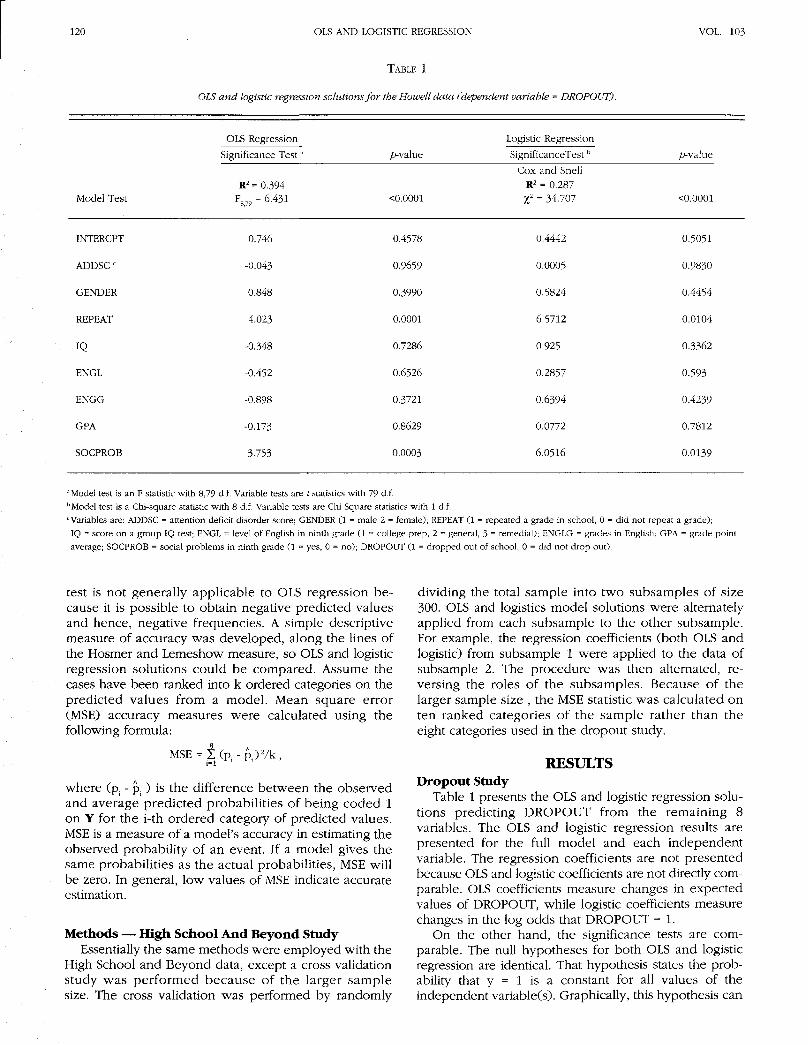
OLS and logistic regression solutions for the Howell data (dependent variable = DROPOUT).

Model Test

OLS Regression

Significance Test:

R2 = 0.394F879 - 6.431

/rvalue

<0.0001

Logistic Regression

SignificanceTest b

Cox and SnellR2 = 0.287

t = 34.707

p-va\ue

O.0001

INTERCPT

ADDSC c

GENDER

REPEAT

IQ

ENGL

ENGG

GPA

SOCPROB

0.746

-0.043

0.848

4.023

-0.348

-0.452

-0.898

-0.173

3.753

0.4578

0.9659

0.3990

0.0001

0.7286

0.6526

0.3721

0.8629

0.0003

0.4442

0.0005

0.5824

6.5712

0.925

0.2857

0.6394

0.0772

6.0516

0.5051

0.9830

0.4454

0.0104

0.3362

0.593

0.4239

0.7812

0.0139

"Model test is an F statistic with 8,79 d.f. Variable tests are t statistics with 79 d.f.b Model test is a Chi-square statistic with 8 d.f. Variable tests are Chi Square statistics with 1 d.f.c Variables are: ADDSC = attention deficit disorder score; GENDER (1 = male 2 = female); REPEAT (1 = repeated a grade in school, 0 = did not repeat a grade);IQ = score on a group IQ test; ENGL = level of English in ninth grade (1 = college prep, 2 = general, 3 = remedial); ENGLG = grades in English; GPA = grade pointaverage; SOCPROB = social problems in ninth grade (1 = yes, 0 = no); DROPOUT (1 = dropped out of school, 0 = did not drop out).

test is not generally applicable to OLS regression be-cause it is possible to obtain negative predicted valuesand hence, negative frequencies. A simple descriptivemeasure of accuracy was developed, along the lines ofthe Hosmer and Lemeshow measure, so OLS and logisticregression solutions could be compared. Assume thecases have been ranked into k ordered categories on thepredicted values from a model. Mean square error(MSE) accuracy measures were calculated using thefollowing formula:

MSE = f (p. -p.) 7k,

where (p. - p. ) is the difference between the observedand average predicted probabilities of being coded 1on Y for the i-th ordered category of predicted values.MSE is a measure of a model's accuracy in estimating theobserved probability of an event. If a model gives thesame probabilities as the actual probabilities, MSE willbe zero. In general, low values of MSE indicate accurateestimation.

Methods — High School And Beyond StudyEssentially the same methods were employed with the

High School and Beyond data, except a cross validationstudy was performed because of the larger samplesize. The cross validation was performed by randomly

dividing the total sample into two subsamples of size300. OLS and logistics model solutions were alternatelyapplied from each subsample to the other subsample.For example, the regression coefficients (both OLS andlogistic) from subsample 1 were applied to the data ofsubsample 2. The procedure 'was then alternated, re-versing the roles of the subsamples. Because of thelarger sample size , the MSE statistic was calculated onten ranked categories of the sample rather than theeight categories used in the dropout study.

RESULTSDropout Study

Table 1 presents the OLS and logistic regression solu-tions predicting DROPOUT from the remaining 8variables. The OLS and logistic regression results arepresented for the full model and each independentvariable. The regression coefficients are not presentedbecause OLS and logistic coefficients are not directly com-parable. OLS coefficients measure changes in expectedvalues of DROPOUT, while logistic coefficients measurechanges in the log odds that DROPOUT = 1.

On the other hand, the significance tests are com-parable. The null hypotheses for both OLS and logisticregression are identical. That hypothesis states the prob-ability that y = 1 is a constant for all values of theindependent variable(s). Graphically, this hypothesis can


TABLE 2

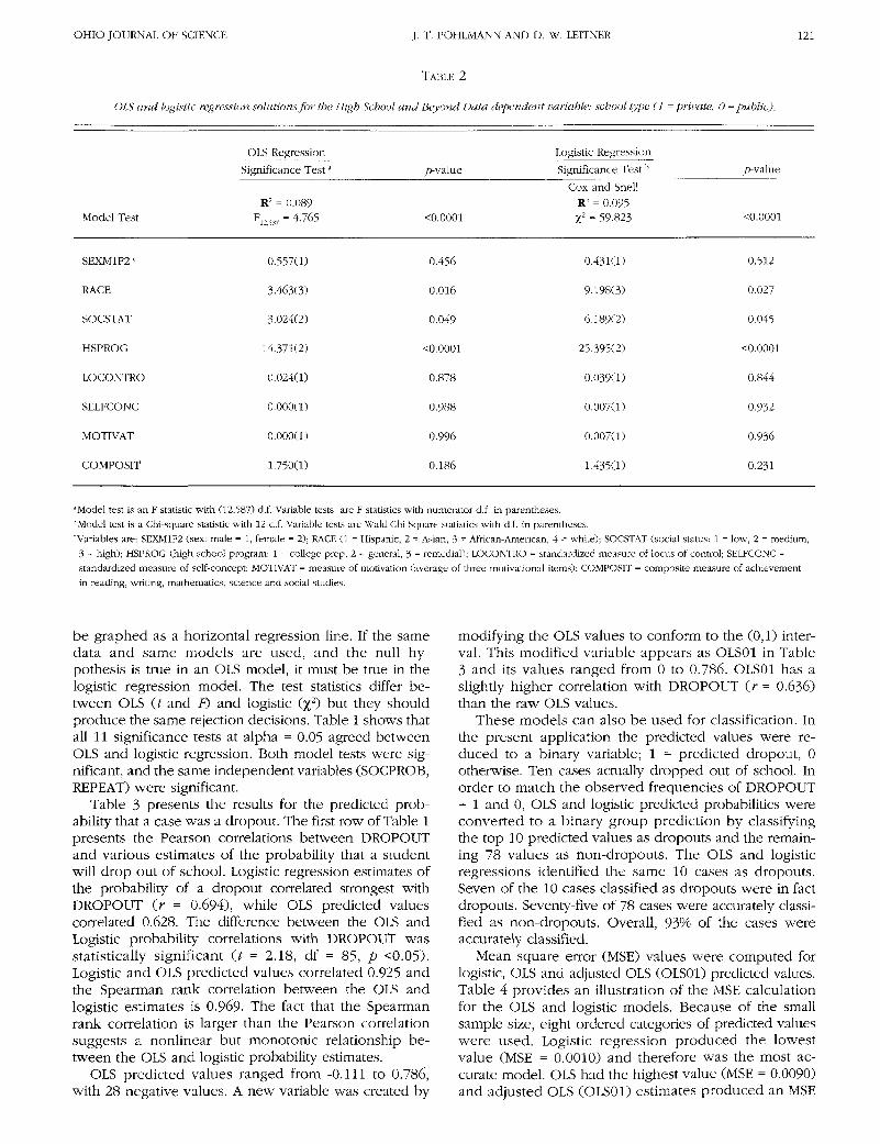
OLS and logistic regression solutions for the High School and Beyond Data dependent variable: school type (1 = private, 0 = public).

Model Test

OLS Regression

Significance Test:

R2 = 0.089F12]587 = 4.765

jf-value

<0.0001

Logistic Regression

Significance Test b

Cox and SnellR2 = 0.095t = 59.823

p-value

<0.0001

SEXM1F2 c

RACE

SOCSTAT

HSPROG

LOCONTRO

SELFCONC

MOTIVAT

COMPOSIT

0.557(1)

3.463(3)

3.024(2)

14.371(2)

0.024(1)

0.000(1)

0.000(1)

1.750(1)

0.456

0.016

0.049

<0.0001

0.878

0.988

0.996

0.186

0.431(1)

9.198(3)

6.189(2)

25.395(2)

0.039(1)

0.007(1)

0.007(1)

1.435(1)

0.512

0.027

0.045

O.0001

0.844

0.932

0.936

0.231

"Model test is an F statistic with (12,587) d.f. Variable tests are F statistics with numerator d.f. in parentheses.hModel test is a Chi-square statistic with 12 d.f. Variable tests are Wald Chi Square statistics with d.f. in parentheses.

'Variables are: SEXM1F2 (sex: male = 1, female = 2); RACE (1 = Hispanic, 2 = Asian, 3 = African-American, 4 = white); SOCSTAT (social status: 1 = low, 2 = medium,

3 = high); HSPROG (high school program: 1 = college prep, 2 = general, 3 = remedial); LOCONTRO = standardized measure of locus of control; SELFCONC =

standardized measure of self-concept; MOTIVAT = measure of motivation (average of three motivational items); COMPOSIT = composite measure of achievement

in reading, writing, mathematics, science and social studies.

be graphed as a horizontal regression line. If the samedata and same models are used, and the null hy-pothesis is true in an OLS model, it must be true in thelogistic regression model. The test statistics differ be-tween OLS it and F) and logistic (%2) but they shouldproduce the same rejection decisions. Table 1 shows thatall 11 significance tests at alpha = 0.05 agreed betweenOLS and logistic regression. Both model tests were sig-nificant, and the same independent variables (SOCPROB,REPEAT) were significant.

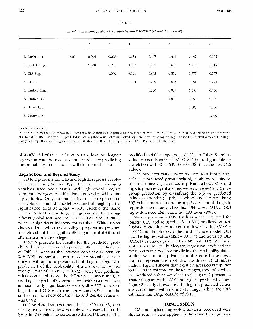
Table 3 presents the results for the predicted prob-ability that a case was a dropout. The first row of Table 1presents the Pearson correlations between DROPOUTand various estimates of the probability that a studentwill drop out of school. Logistic regression estimates ofthe probability of a dropout correlated strongest withDROPOUT (r = 0.694), while OLS predicted valuescorrelated 0.628. The difference between the OLS andLogistic probability correlations with DROPOUT wasstatistically significant it = 2.18, df = 85, p <0.05).Logistic and OLS predicted values correlated 0.925 andthe Spearman rank correlation between the OLS andlogistic estimates is 0.969. The fact that the Spearmanrank correlation is larger than the Pearson correlationsuggests a nonlinear but monotonic relationship be-tween the OLS and logistic probability estimates.

OLS predicted values ranged from -0.111 to 0.786,with 28 negative values. A new variable was created by

modifying the OLS values to conform to the (0,1) inter-val. This modified variable appears as OLS01 in Table3 and its values ranged from 0 to 0.786. OLS01 has aslightly higher correlation with DROPOUT (r = 0.636)than the raw OLS values.

These models can also be used for classification. Inthe present application the predicted values were re-duced to a binary variable; 1 = predicted dropout, 0otherwise. Ten cases actually dropped out of school. Inorder to match the observed frequencies of DROPOUT= 1 and 0, OLS and logistic predicted probabilities wereconverted to a binary group prediction by classifyingthe top 10 predicted values as dropouts and the remain-ing 78 values as non-dropouts. The OLS and logisticregressions identified the same 10 cases as dropouts.Seven of the 10 cases classified as dropouts were in factdropouts. Seventy-five of 78 cases were accurately classi-fied as non-dropouts. Overall, 93% of the cases wereaccurately classified.

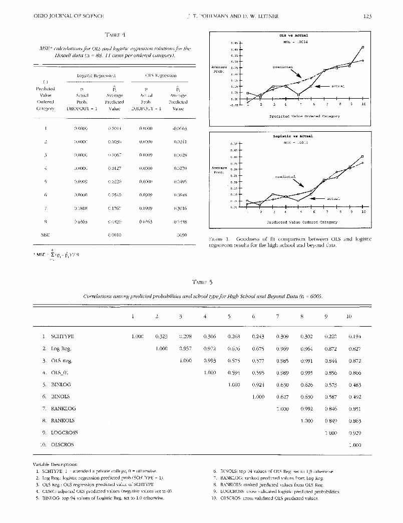
Mean square error (MSE) values were computed forlogistic, OLS and adjusted OLS (OLS01) predicted values.Table 4 provides an illustration of the MSE calculationfor the OLS and logistic models. Because of the smallsample size, eight ordered categories of predicted valueswere used. Logistic regression produced the lowestvalue (MSE = 0.0010) and therefore was the most ac-curate model. OLS had the highest value (MSE = 0.0090)and adjusted OLS (OLS01) estimates produced an MSE


TABLE 3

Correlations among predicted probabilities and DROPOUT (Howell data, n = 88).

3. 5. 6.

1. DROPOUT

2. Logistic Reg.

3. OLS Reg.

4. OLS01

5. Ranked Log.

6. Ranked OLS

7. Binary Log.

8. Binary OLS

1.000 0.694

1.000

0.628

0.925

1.000

0.636

0.937

0.994

1.000

0.467

0.702

0.832

0.789

1.000

0.444

0.695

0.850

0.803

0.969

1.000

0.662

0.914

0.777

0.791

0.550

0.550

1.000

0.662

0.914

0.777

0.791

0.550

0.550

1.000

1.000

Variable Descriptions:

DROPOUT: 1 = dropped out of school, 0 = did not drop; Logistic Reg.: logistic regression predicted prob. (DROPOUT = 1); OLS Reg.: OLS regression predicted value

of DROPOUT; OLS01: adjusted OLS predicted values (negative values set to 0); Ranked Log.: ranked values of Logistic Reg.; Ranked OLS: ranked values of OLS Reg.;

Binary Log.: top 10 values of Logistic Reg. set to 1,0 otherwise; Binary OLS: top 10 values of OLS Reg. set to 1,0 otherwise.

of 0.0078. All of these MSE values are low, but logisticregression was the most accurate model for predictingthe probability that a student will drop out of school.

High School and Beyond StudyTable 2 presents the OLS and logistic regression solu-

tions predicting School Type from the remaining 8variables. Race, Social Status, and High School Programwere multicategory classifications and coded with dum-my variables. Only the main effect tests are presentedin Table 4. The full model test and all eight partialsignificance tests at alpha = 0.05 yielded the sameresults. Both OLY and logistic regression yielded a sig-nificant global test; and RACE, SOCSTAT and HSPROGwere the significant independent variables. White, upperclass students who took a college preparatory programin high school had significantly higher probabilities ofattending a private college.

Table 5 presents the results for the predicted prob-ability that a case attended a private college. The first rowof Table 5 presents the Pearson correlations betweenSCHTYPE and various estimates of the probability that astudent will attend a private school. Logistic regressionpredictions of the probability of a dropout correlatedstrongest with SCHTYPE (r= 0.323), while OLS predictedvalues correlated 0.298. The difference between the OLSand Logistic probability correlations with SCHTYPE wasnot statistically significant (t = 0.89, df = 597, p >0.05).Logistic and OLS estimates correlated 0.957, and therank correlation between the OLS and logistic estimateswas 0.992.

OLS predicted values ranged from -0.15 to 0.35, with47 negative values. A new variable was created by modi-fying the OLS values to conform to the (0,1) interval. This

modified variable appears as OLS01 in Table 5 and itsvalues ranged from 0 to 0.35. OLS01 has a slightly highercorrelation with SCHTYPE (r = 0.306) than the raw OLSvalues.

The predicted values were reduced to a binary vari-able; 1 = predicted private school, 0 otherwise. Ninety-four cases actually attended a private school. OLS andlogistic predicted probabilities were converted to a binarygroup prediction by classifying the top 94 predictedvalues as attending a private school and the remaining503 values as not attending a private school. Logisticregression accurately classified 484 cases (81%). OLSregression accurately classified 480 cases (80%).

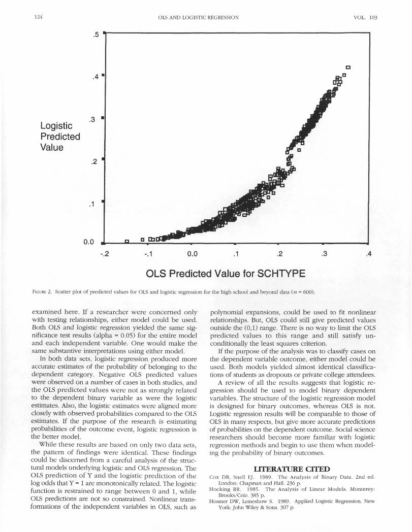
Mean square error (MSE) values were computed forlogistic, OLS, and adjusted OLS (OLS01) predicted values.Logistic regression produced the lowest value (MSE =0.0011) and therefore was the most accurate model. OLShad the highest value (MSE = 0.0034) and adjusted OLS(OLS01) estimates produced an MSE of .0029. All theseMSE values are low, but logistic regression produced themost accurate model for predicting the probability that astudent will attend a private school. Figure 1 provides agraphic representation of this goodness of fit infor-mation. Figure 1 shows that logistic regression is superiorto OLS in the extreme prediction ranges, especially whenthe predicted values are close to 0. Figure 2 presents ascatter diagram of the OLS and logistic predicted values.Figure 2 clearly shows how the logistic predicted valuesare constrained within the (0,1) range, while the OLSestimates can range outside of (0,1).

DISCUSSIONOLS and logistic regression analysis produced very

similar results when applied to the same two data sets


TABLE 4

MS/:" calculations for OLS and logistic regression solutions for the

Howell data (n = 88, 11 cases per ordered category).

(i)

Predicted

Value

Ordered

Category

1

2

3

4

5

6

7

8

MSE

Logistic Regression

P,ActualProb.

DROPOUT = 1

0.0000

0.0000

0.0000

0.0000

0.0909

0.0000

0.1818

0.6363

A

Pi

Average

Predicted

Value

0.0014

0.0036

0.0067

0.0127

0.0220

0.0540

0.1767

0.6320

0.0010

OLS Regression

P,ActualProb.

DROPOUT =

0.0000

0.0000

0.0909

0.0000

0.0000

0.0909

0.0909

0.6363

= 1

A

Pi

Average

Predicted

Value

-0.0663

-0.0241

0.0028

0.0270

0.0495

0.0848

0.3016

0.5338

.0090

Averaae 0.25 •-Prob.

OLS vs Actual

MSE = .0034

I I 1 1 1 1 1 1

Loo i s t i c vs Actual

MSE = .0011

FIGURE 1. Goodness of fit comparison between OLS and logisticregression results for the high school and beyond data.

8

MSE = I(p_- p,.) 7 8

TABLE 5

Correlations among predicted probabilities and school type for High School and Beyond Data (n = 600).

1 3 4 6 7 10

1. SCHTYPE

2. Log Reg.

3. OLS Reg.

4. OLS_01

5. BINLOG

6. BINOLS

7. RANKLOG

8. RANKOLS

9. LOGCROSS

10. OLSCROS

1.000 0.323 0.298

1.000 0.957

1.000

0.306

0.972

0.993

1.000

0.268

0.676

0.575

0.594

1.000

0.243

0.675

0.577

0.595

0.924

1.000

0.309

0.969

0.985

0.989

0.630

0.627

1.000

0.302

0.964

0.991

0.995

0.626

0.630

0.992

1.000

0.220

0.872

0.844

0.856

0.573

0.587

0.846

0.849

1.000

0.194

0.827

0.872

0.866

0.483

0.492

0.851

0.863

0.929

1.000

Variable Descriptions:

1. SCHTYPE: 1 = attended a private college, 0 = otherwise.

2. Log Reg.: logistic regression predicted prob.(SCHTYPE = 1).

3. OLS Reg.: OLS regression predicted value of SCHTYPE.

4. OLS01: adjusted OLS predicted values (negative values set to 0).

5. BINLOG: top 94 values of Logistic Reg. set to 1,0 otherwise.

6. BINOLS: top 94 values of OLS Reg. set to 1,0 otherwise.

7. RANKLOG: ranked predicted values from Log Reg.

8. RANKOLS: ranked predicted values from OLS Reg.

9. LOGCROSS: cross validated logistic predicted probabilities.

10. OLSCROS: cross validated OLS predicted values.


LogisticPredictedValue

-.2 -.1 o.o .1 .2 .3 .4

OLS Predicted Value for SCHTYPE

FIGURE 2. Scatter plot of predicted values for OLS and logistic regression for the high school and beyond data (n = 600).

examined here. If a researcher were concerned onlywith testing relationships, either model could be used.Both OLS and logistic regression yielded the same sig-nificance test results (alpha = 0.05) for the entire modeland each independent variable. One would make thesame substantive interpretations using either model.

In both data sets, logistic regression produced moreaccurate estimates of the probability of belonging to thedependent category. Negative OLS predicted valueswere observed on a number of cases in both studies, andthe OLS predicted values were not as strongly relatedto the dependent binary variable as were the logisticestimates. Also, the logistic estimates were aligned moreclosely with observed probabilities compared to the OLSestimates. If the purpose of the research is estimatingprobabilities of the outcome event, logistic regression isthe better model.

While these results are based on only two data sets,the pattern of findings were identical. These findingscould be discerned from a careful analysis of the struc-tural models underlying logistic and OLS regression. TheOLS prediction of Y and the logistic prediction of thelog odds that Y = 1 are monotonically related. The logisticfunction is restrained to range between 0 and 1, whileOLS predictions are not so constrained. Nonlinear trans-formations of the independent variables in OLS, such as

polynomial expansions, could be used to fit nonlinearrelationships. But, OLS could still give predicted valuesoutside the (0,1) range. There is no way to limit the OLSpredicted values to this range and still satisfy un-conditionally the least squares criterion.

If the purpose of the analysis was to classify cases onthe dependent variable outcome, either model could beused. Both models yielded almost identical classifica-tions of students as dropouts or private college attendees.

A review of all the results suggests that logistic re-gression should be used to model binary dependentvariables. The structure of the logistic regression modelis designed for binary outcomes, whereas OLS is not.Logistic regression results will be comparable to those ofOLS in many respects, but give more accurate predictionsof probabilities on the dependent outcome. Social scienceresearchers should become more familiar with logisticregression methods and begin to use them when model-ing the probability of binary outcomes.

LITERATURE CITEDCox DR, Snell EJ. 1989. The Analysis of Binary Data. 2nd ed.

London: Chapman and Hall. 236 p.Hocking RR. 1985. The Analysis of Linear Models. Monterey:

Brooks/Cole. 385 p.Hosmer DW, Lemeshow S. 1989- Applied Logistic Regression. New

York: John Wiley & Sons. 307 p.


Howell DC. 2002. Statistical Methods for Psychology. 5th ed. Pacific series no. 07-106. Thousand Oaks (CA): Sage. 98 p.Grove (CA): Duxbury. p 728-31. National Center for Education Statistics. 1995. Statistical Analysis

King EN, Ryan TP. 2002. A preliminary investigation of maximum Report January 1995 High School and Beyond: 1992 Descrip-likelihood logistic regression versus exact logistic regression. tive Summary of 1980 High School Sophomores 12 Years Later.American Statistician 56(3): 163-70. Washington: US Dept of Education. 112 p.

Menard S. 1995. Applied logistic regression analysis. Sage Univ SAS Institute Inc. 1989- SAS/STAT User's Guide. Version 6, 4th ed.,Paper series on Quantitative Applications in the Social Sciences vol. 2. Cary (NC): SAS Institute. 846 p.

a comparison of ordinary least squares and logistic regression · inant analysis and ols, logistic...

Documents