a comparative study of clustering methods for active region detection in solar euv images
TRANSCRIPT

Solar Phys (2013) 283:691–717DOI 10.1007/s11207-013-0239-2
A Comparative Study of Clustering Methods for ActiveRegion Detection in Solar EUV Images
C. Caballero · M.C. Aranda
Received: 10 January 2012 / Accepted: 21 January 2013 / Published online: 15 February 2013© Springer Science+Business Media Dordrecht 2013
Abstract The increase in the amount of solar data provided by new satellites makes it nec-essary to develop methods to automate the detection of solar features. Here we present amethod for automatically detecting active regions in solar extreme ultraviolet (EUV) imagesusing a series of steps. Initially, the bright regions in the image are segmented using seededregion growing. In a second phase these bright regions are clustered into active regions.Partition-based clustering (both hard and fuzzy) and hierarchical clustering are compared inthis work. The aim of the clustering phase is to associate a group to each segmented regionin order to reduce the total number of active regions. This facilitates the documentation orsubsequent monitoring of these regions. We use two indicators to validate the partitioning:i) the number of detected clusters approximates the number of active regions reported bythe National Oceanic and Atmospheric Administration (NOAA) and ii) the area that defineseach cluster overlaps with the area of an active region of NOAA. Experiments have beenperformed on over 6000 images from SOHO/EIT (195 Å). The best results were obtainedusing hierarchical clustering. The method detects a set of active regions in an image of thesolar corona that successfully matches the number of NOAA regions. We will use theseregions to perform real-time monitoring and flare detection.
Keywords Active region · Clustering method · Segmentation
1. Introduction
The automatic processing of information in solar physics is becoming increasingly importantdue to the substantial increase in the size of solar image data archives. The Solar Dynam-ics Observatory (SDO; Pesnel, Thompson, and Chamberlin, 2012) generates around 1TB
C. Caballero (�) · M.C. ArandaDepartment of Languages and Computer Science, Engineering School, University of Malaga, C/ DoctorOrtiz Ramos s/n, 29071 Málaga, Spaine-mail: [email protected]
M.C. Arandae-mail: [email protected]
692 C. Caballero, M.C. Aranda
of data a day, which cannot be treated manually. To make good use of all this informa-tion, an effective solution is to use automated feature-detection methods that allow users toselectively acquire interesting portions of the full data set.
The automatic detection of active regions (ARs) is a particularly interesting problem be-cause most solar activity, such as flares and coronal mass ejections, occurs in these regions.According to Ridpath (2012), an active region is an area on the Sun where strong magneticfields emerge through the photosphere into the chromosphere and corona. Active regionsobserved in the photosphere often include sunspots and faculae. Plague regions that appearin the chromosphere are also often associated with ARs. In the corona, ARs have enhanceddensity and temperature, appearing bright in X-ray and ultraviolet images.
Active regions are allocated numbers by the National Oceanic and Atmospheric Ad-ministration (NOAA) in order of appearance. According to NOAA, an active region mustbe observed by two observatories before it is given a number; although a region may benumbered before its presence is confirmed by another observatory if a flare is observed tooccur in it. Although NOAA groups sunspots in continuum images, isolated active regionsare closely related to activity in other frequency bands, for example in Hα (Zharkov andZharkova, 2011) or EUV (Sych et al., 2009).
The problem of coronal image segmentation in general, and the detection and track-ing of regions of interest in solar images in particular, has been addressed in many waysin recent years. The principal segmentation methods can be classified into two main ap-proaches: edge-based methods and region-based methods. A comprehensive review of theliterature on edge-based methods can be found in Veronig et al. (2000), Fuller, Aboudarham,and Bentley (2005), Robbrecht, Berghmans, and van der Linden (2006), and Young andGallagher (2008). Region-based methods are divided into thresholding techniques andregion growing methods. Both have been extensively applied in solar image process-ing. The former have been used for the detection of sunspots (Zharkov et al., 2004;Colak and Qahwaji, 2008), filaments (Aboudarham et al., 2008; Joshi, Srivastava, andMathew, 2010), coronal holes (Nieniewski, 2004; Krista and Gallagher, 2009) and ac-tive regions (Barra et al., 2009). The seeded region growing method has been widelyused for identification and tracking of active regions. The works vary in the way seedsare selected. Various techniques use a simple static threshold (McAteer et al., 2005;Qahwaji and Colak, 2006), statistic-based local thresholding (Benkhalil et al., 2006) or us-ing two consecutive magnetogram images (Higgins et al., 2010).
Clustering techniques have not been widely applied to solar data. The goal of clusteringis to reduce the amount of data by categorizing or grouping similar features in a data set. TheSpatial Possibilistic Clustering Algorithm (SPoCA; Barra, Delouille, and Hochedez, 2008)uses a multi-channel unsupervised spatially-constrained fuzzy clustering procedure. The al-gorithm segments EUV solar images into regions corresponding to active regions (AR),coronal holes (CH), and the quiet Sun (QS). Fuzzy clustering has also been used in Arandaand Caballero (2010) to achieve robust automatic detection of active regions in EUV solarimages. On the other hand, Colak and Qahwaji (2009) present a method to identify, groupand sort sunspots. To group sunspots, they use an ad hoc clustering technique, but proposeto improve their method by using statistical clustering. In addition, Nguyen et al. (2006)have made a comparative study of the hierarchical clustering and density-based clusteringmethods applied to the identification and classification of sunspots.
In this work, we focus on detecting active regions in EUV solar images. In the context ofthis work NOAA’s definition of AR is used. Our procedure is based on region growing seg-mentation and hierarchical clustering. It is fast and stable when running on image sequencesover time. This work is included in a larger project aimed at tracking these active regionsand detecting flares.
Clustering Methods for Active Region Detection in Solar EUV Images 693
The rest of this paper is organized as follows: Section 2 describes the methods used in thiswork. Some experimental results are presented in Section 3, comparing different clusteringmethods and validity indices. We conclude in Section 4.
2. Methods
Our system is divided into several stages:
i) segmentation,ii) clustering, and
iii) cluster validity.
The segmentation determines those pixels in the image where there are bright regions. Inthe clustering phase, the bright regions are grouped into active regions. Finally, the validationphase determines whether the active regions have been clustered correctly.
The segmentation method presented in this article is based on a seeded region growingsegmentation. This new method for the segmentation of solar EUV images is described inSection 2.1.
The segmented regions are grouped into sets whose components are similar accordingto a criterion of proximity. Grouping is performed using clustering techniques. Clusteringmethods (Anderberg, 1973; Hartigan, 1975; Jain and Dubes, 1988; Xu and Wunsch, 2008;Ghaemi et al., 2009) can be divided into two basic types: hierarchical and partition-basedclustering. Within each of the types is a wealth of subtypes and different algorithms forfinding the clusters. Hierarchical clustering proceeds successively by either merging smallerclusters into larger ones, or by splitting larger clusters. Partition-based clustering, on theother hand, attempts to directly decompose the data set into a set of disjoint clusters. Thecriterion function that the clustering algorithm tries to minimize may emphasize the localstructure of the data. Neither hierarchical nor partition-based methods directly address theissue of determining the number of groups within the data. Some validity indices have beenused for this purpose, which depend on the type of clustering. These are defined based onstatistical concepts such as the distance within the cluster or the distance between clusters(Halkidi, Batistakis, and Varzigiannis, 2002a, 2002b).
Section 2.2 reviews some clustering methods while Section 2.3 presents some validityindices to be used along with each clustering method.
2.1. Segmentation: GSRG2h Method
This section describes our method called global seeded region growing based on the geom-etry of the histogram (GSRG2
h) for solar EUV image segmentation, which is a variant of aseeded region growing (SRG) method. The output is a set of bright regions or regions ofinterest (ROIs). This technique is based on the histogram of the image and consists of threephases: i) a new procedure of seed selection is used (Section 2.1.1), ii) SRG is applied usingthe previously selected seeds (Section 2.1.2), and iii) regions derived from noisy seeds areremoved (Section 2.1.3).
2.1.1. Seed Selection: A Geometrical Method
The aim of this phase is to select a set of pixels (seeds) on which to apply SRG. Seedselection is important because it determines the outcome of the region growing and therefore

694 C. Caballero, M.C. Aranda
Figure 1 Histogram derivedfrom a solar image fromSOHO/EIT (195 Å) instrumenttaken on 3 August 2000. Thehistogram shows the thresholdselected by the method GSRG2
h.The polynomial fit is overplottedin red.
the final segmentation. The seeds can be selected from a threshold on the histogram. Thosepixels with values above this threshold will be selected as seeds.
In our previous work (Aranda and Caballero, 2010), we used the optimal value ofOtsu (1979) as the threshold for selecting the seeds. It is a statistical value that is widelyaccepted in the literature for histogram-based segmentation using a threshold. It gives goodresults in the segmentation of most images. The study was made on 400 images, and in70 % of them the regions were identified correctly. But the biggest drawback of the optimalvalue of Otsu, as with the mean and median (but less so), is that the final result is affectedby outliers. These outliers change the optimal value of Otsu by making the ROIs appear ordisappear.
In this work we have developed a new technique of seed selection that is not based oneither a local or global statistical measurement, but is based on the geometry or shape of thehistogram of the solar image. In it, most pixels have a value close to zero, so that pixels withthe highest values in the histogram have few occurrences. As Figure 1 shows, the histogramdecreases toward higher intensity values, and therefore, the line segment that connects thesepoints has a decreasing slope. If the threshold value is determined at the beginning of the fallof the histogram, then the level of intensity of the selected pixels will be too low. This meansirrelevant pixels (noise) are taken as relevant objects. On the other hand, if the thresholdvalue is determined at the end of the fall of the histogram, then relevant objects are taken asnoise. Therefore, the ideal threshold is close to the beginning of the fall, and not just at thebeginning. Here we list the steps of the seed selection method:
1. Calculate the functions that perform the first degree polynomial fit and its slope over thepoints of the histogram of a SOHO/EIT (Delaboudiniére et al., 1995) solar image.
2. Seek histogram points over which the slopes of the lines of several points are small (thosein which the value of slope is less than 10−7. The slope has the dimension of the y-axisunit (number of pixels) divided by the x-axis unit (intensity value).
3. Filter the previous points to select those that are in a stable zone of the histogram. A por-tion of the histogram is considered stable when the slope of two groups of histogrampoints is in the range [−5,0].
4. Select the first point of the stable zone as the threshold to select the seeds.5. Select the seeds as the pixels with values greater than the threshold.
This technique generates a dynamic threshold that adapts to each image. The calculationis stable in noisy images. It is also stable in images with large differences in brightness, such

Clustering Methods for Active Region Detection in Solar EUV Images 695
as if a flare occurs in one of the active regions. This is shown in Section 3.4. Disadvantagesof the method are that it is slower than other techniques and cannot be used with imageswhose histogram has been manipulated. Appendix A shows the pseudocode of the seedselection method.
2.1.2. Seeded Region Growing
Segmentation methods based on seeded region growing (Adams and Bischof, 1994) useinformation from the neighborhood of each pixel. The basic idea is that the pixels in thesame neighborhood have similar statistical properties and belong to the same region.
This method uses a set of n seeds (the points selected in the previous phase (Sec-tion 2.1.1)), and each of these seeds initially belongs to a different set Ai . The method addsa pixel onto the edge of one of the sets Ai in each step. Furthermore, each added pixel isconsidered as a new seed. The iterative process will select all the pixels near each seed thathave similar properties. Several initial seeds can generate the same region when the iterativeprocess selects all the pixels that form a path between two pixels.
The output is a set of regions Ai with similar intensity properties. The resulting regionsdepend largely on the seeds, because these pixels create the relevant regions in the image.SRG is very sensitive to noisy images, because if noisy pixels are selected as seeds then theerror is propagated. Therefore, the method is fast and robust if the seeds are suitable for theimage. Appendix B shows the pseudocode of this technique.
2.1.3. Selection of Regions of Interest
After applying the region growing method, there may be some noisy regions in the image.Therefore, a more satisfactory result is achieved after a region selection phase that consistsof two steps:
1. First, a thresholding is performed based on the area of regions. This eliminates regionsderived from noisy seeds (regions with a size less than 10 pixels).
2. Once large regions have been selected (regions with a size greater than 75 pixels), thenext step is to look for regions close to these (those with a distance of less than 25 pixelsaway), regardless of the size of the surrounding regions.
Figure 2(a) shows an unprocessed image of the Sun taken on 15 January 2005 with theSOHO satellite, and Figure 2(b) shows the final result of the segmentation of this image.
2.2. Clustering to Obtain Active Regions
Segmented regions obtained from the preceding stage will be grouped into active regions.We use clustering for this purpose. The goal is to combine sets of objects into subsets (clus-ters) so that objects in the same cluster are similar to a certain degree. The clustering is basedon information that describes the objects and the relationship between objects. Therefore,the first step is to determine how to describe each region (whether only one object or several)and how to measure the relationship between them, i.e. how to define the similarity betweentwo objects. This will be discussed in Section 2.2.1.
An analysis of the main clustering methods is performed in this work to resolve whichclustering method to use to form the active regions. Clustering methods are basically dividedinto partition-based and hierarchical: the former type is subdivided into hard and fuzzy.Figure 3 shows an outline of the techniques compared in this work. Each of these types willbe described in Sections 2.2.2 (partition-based hard clustering), 2.2.3 (partition-based fuzzyclustering) and 2.2.4 (hierarchical clustering).

696 C. Caballero, M.C. Aranda
Figure 2 (a) Unprocessed image of the Sun taken on 15 January 2005 with the SOHO/EIT (195 Å) instru-ment. (b) Image segmented using the GSRG2
h method.
Figure 3 Several clustering methods. The methods used in this paper are shown by thick black frames.

Clustering Methods for Active Region Detection in Solar EUV Images 697
Figure 4 Three characterizations of the ROIs (a) using the centroids, (b) using all data points, and (c) usingthe edges of each region.
2.2.1. Characterization of the Problem
The input to the clustering process is composed of those points selected from each ROI.These are the objects to be grouped. One possible solution is to select a single point ineach region, such as the centroid (weighted area). Most of the methods are computationallyfeasible using this solution. However, the set of points selected is too small. This makes itdifficult to perform the clustering correctly. Another solution is to select all of the points inthe regions. In this case, most methods are not computationally feasible. A final possibilityis to select the points at the edge of each region. This solution is used in enough points toperform the clustering without a high computational cost. The latter solution is used in thiswork. Figure 4 shows an EUV image of 15 January 2005 with three possible characteriza-tions of the ROIs.
The similarity between objects is measured differently, depending on the type of cluster-ing. Both partition-based and hierarchical clustering are based on the proximity of objects.Therefore the dissimilarity measure can be calculated as a distance function (the greaterthe distance, the greater the dissimilarity between objects). Some commonly used distance
698 C. Caballero, M.C. Aranda
functions are the Euclidean distance, the Manhattan distance, the maximum distance andthe Mahalanobis distance. The choice of an appropriate function will influence the shapeof the clusters, as some elements may be close to one another according to one distancemeasure and farther away according to another. We have chosen the Euclidean distance inthis work, but a further study could be carried out to investigate which would be more ap-propriate.
2.2.2. Partition-Based Hard Clustering
Partitioning clustering methods obtain a single partition of the set by moving objects itera-tively from one cluster to another, starting from an initial partition. The number of clustershas to be specified in advance and typically does not change during the course of the clus-tering process.
Hard clustering methods are a subclass of partitioning methods in which each object canonly belong to a cluster. Each cluster may be represented by a centroid or a representativecluster that may not necessarily be a member of the data set. This is a sort of summarydescription of all the objects contained in a cluster. The precise form of this description willdepend on the type of object that is being clustered. In our case, the arithmetic mean of allobjects within a cluster serves as an appropriate representative.
When the number of clusters is fixed to k, the k-means clustering gives a formal defini-tion as an optimization problem: find k cluster centroids and assign the objects to the nearestcluster centroid, such that the distances from the cluster are minimized. The objective func-tion to be minimized is given by
J (X,V ) =k∑
j=1
n∑
i=1
d(X
(j)
i , Vj
), (1)
where X = {x1, x2, . . . , xn} are the objects to be classified, V = [v1, v2, . . . , vc] is the vectorof centroids. The distance function d is calculated between the i-th point of the j -th clusterand the reference point of the j -th cluster. The vector of centroids is initiated randomly.
From Equation (1) a family of clustering methods arises that is determined according tothe following conditions: the initial reference point of each cluster, the dissimilarity functionused by the clustering method, and the method used to select the new reference points foreach cluster.
Due to the high computational cost of solving this problem, the common approach is tosearch only for approximate solutions. A particularly well-known approximation algorithmis the k-means algorithm (Steinhaus, 1956; Macqueen, 1967). It only finds a local optimumhowever, and is commonly run multiple times with different random initializations. Vari-ations of k-means often include such optimizations as choosing the best of multiple runs,but also restricting the centroids to members of the data set (k-medoids) (Kaufman andRousseeuw, 1987), choosing medians (k-medians clustering) or choosing the initial centersless randomly (K-means++) (Arthur and Vassilvitskii, 2007).
Most k-means-type algorithms require the number of clusters (k) to be specified in ad-vance, which is considered to be one of the biggest drawbacks of these algorithms. Fur-thermore, the algorithms prefer clusters of approximately similar size, as they will alwaysassign an object to the nearest centroid. This often leads to incorrect divisions between clus-ters. Another important drawback is that these algorithms are very sensitive to outliers thatcan distort centroid positions. Finally, and as mentioned above, these algorithms often termi-nate at a local optimum, which may mean the most appropriate solutions are not identified.
Clustering Methods for Active Region Detection in Solar EUV Images 699
All of these drawbacks directly affect our solution, since the active regions generally do nothave a particular form or a similar size. Also, the images may contain noise that affects thecalculation of the centroids and the final partition.
2.2.3. Partition-Based Fuzzy Clustering
Fuzzy clustering methods are also partition-based methods, but in fuzzy clustering the ob-jects belong to all clusters with a varying degree of membership. Fuzzy methods are veryuseful when the boundaries of different clusters are not clearly delimited. They minimizethe membership function described in Equation (2), which is similar to the one defined inEquation (1) but with the difference that the membership matrix (μ) appears.
J (X;U,V ) =c∑
i=1
M∑
k=1
(μik)md(xk, vi), (2)
where X is for the data to be classified, V is the vector of reference points and U = [μik] ∈Mfc is the membership matrix of X. Let m ∈ [1,∞) be the fuzzification parameter. A morediffuse component occurs when m is a large value. In contrast, the method is hard when thevalue of m is close to 1, because objects can only belong to one cluster.
Three of the main fuzzy clustering techniques are fuzzy c-means (FCM) (Bezdek, 1981),Gustafson–Kessel (1978), and Gath–Geva (1989). A brief explanation of each method andthe differences between them is presented below.
Gustafson–Kessel (GK) extends the FCM method with a different norm for each cluster,thus optimizing the shape (overlapped area) of the clusters while keeping the number ofobjects of each cluster (volume) constant. This clustering method is perfectly adequate foridentifying clusters without a predetermined geometric shape, although they must have aconstant volume. It is also relatively insensitive to the initial values of the partition matrixin comparison with other similar methods.
However, this method has some drawbacks: i) the computational cost is quite high, al-though Babuska (2002) provides an alternative to improve the estimation of the variance;ii) GK can detect clusters of different geometric shapes, although clusters actually have ahyper-ellipsoidal shape, so that it really is ideal for hyper-ellipsoidal clusters of the samesize; iii) the clusters must have the same volume; and iv) numerical problems may arisewhen the number of data is small or data are linearly dependent because the covariance ma-trix is almost singular. Nevertheless, in Aranda and Caballero (2010) the Gustafson–Kesselalgorithm was used to detect solar ARs because the shape of the clusters was not knowna priori and the clusters had the same volume. It was shown that this method is not suited toregions that are not constant in volume.
The Gath–Geva (GG) method is an extension of the GK method, which takes the size anddensity into account. The GG method introduces an exponential term and uses the measuregiven by Bezdek and Dunn (1975). This method detects clusters of different sizes, shapesand densities. However, it depends on a good initialization. In contrast to the FCM methodand the GK method, the GG method is not based on an objective function, but it is a fuzzi-fication of statistical estimators.
The c-means method of clustering has the same drawbacks as the hard k-means method.It is sensitive to noisy images, because the noise can affect the calculation of the centroidsand therefore the partition in active regions. Furthermore, the method determines the shapeof clusters and their size, which must be similar for all clusters.

700 C. Caballero, M.C. Aranda
Figure 5 The distance between clusters may be (a) single link, (b) complete link, or (c) average link.
2.2.4. Hierarchical Clustering
Hierarchical clustering (or connectivity-based clustering) is based on the core idea of objectsbeing more related to nearby objects than to objects farther away. As such, these algorithmsconnect objects to form clusters based on their distance. Techniques for hierarchical cluster-ing generally fall into two types: both were developed by Kaufman and Rousseeuw (1990).
The first technique is called divisive analysis (DIANA) in which there is initially a singlelarge group including all of the objects. This large group is broken down into subgroups ateach step. This method has a high computational cost since its order of complexity is O(2N).This is because, for a cluster with N objects, it is necessary to construct 2(N−1) − 1 possiblesub-clusters.
The other technique is called agglomerative nesting (AGNES) in which each object isinitially a cluster. In each iteration the closest clusters are merged into one cluster untilall objects belong to the same cluster. The major drawback of this technique is its highcomputational cost as its order of complexity is O(N2), although this technique has a lowercomputational cost than DIANA. There are other variations of this technique to minimizethe order of complexity.
In order to decide which clusters should be combined (for agglomerative) or split (for di-visive analysis), a measure of distance between clusters is required. This is achieved by usinga distance function between pairs of objects (see Section 2.2.1), and a linkage criterion thatspecifies the distance of clusters as a function of the pairwise distances of objects in the clus-ters. Some commonly used linkage criteria are: single-linkage clustering (minimizing objectdistances), complete linkage clustering (maximizing object distances), or unweighted pairgroup method with arithmetic mean (UPGMA, also known as average linkage clustering).Figure 5 shows the distance between clusters using single link, complete link and averagelink.
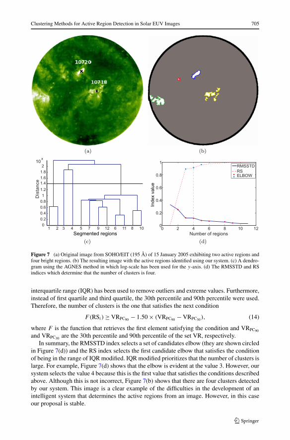
Hierarchical clustering does not provide a single partitioning of the data set, but insteadprovides an extensive hierarchy of clusters that merge with each other at certain distances.Therefore the results are usually presented in a binary tree or dendrogram. In a dendrogram,the y-axis marks the distance at which the clusters merge, while the objects are placed alongthe x-axis such that the clusters do not mix. Figure 7(c) shows the dendogram of a solarEUV image of 15 January 2005 using the AGNES method in which log-scale has been usedfor the y-axis.
The hierarchical clustering has the following advantages:
i) the robustness against outliers;ii) configuration or initialization parameters are not needed; and
iii) clusters must not have a specific geometric shape.
It has the disadvantage of being computationally expensive, although the reduction ofpoints in the region by selecting only the edge points makes this method computationallyaffordable for this problem.

Clustering Methods for Active Region Detection in Solar EUV Images 701
Figure 6 (a – b) Cohesion and separation calculated between all the objects together. (c – d) Cohesion andseparation calculated between all the objects together and a reference point.
2.3. Determining the Number of Clusters: Cluster Validity
Neither hierarchical nor partition-based methods directly address the issue of determiningthe number of clusters within the data. A validity index provides an objective measurementof a cluster result. The number of clusters suitable for all data is determined by the optimumvalue of the validity index. Developing these indices is a complicated task. The problemis simplified if the shape (circular, elliptical, linear, etc.) or the volume of the data set isknown.
Most validity indices have been developed based on the concepts of cohesion and sep-aration. The cohesion measures how closely related are objects in a cluster. Clusters arecompact when cohesion is high. On the other hand, the separation indicates how distinctor well-separated a cluster is from the other clusters. Both measurements can be calculatedbetween the objects themselves or between objects and a reference point. Figure 6 showsthe cohesion and separation measurements.
The concepts of cohesion and separation calculated between the objects together andbetween objects and a reference point, respectively, are given by
cohesion(Ci) =∑
x,y∈Ci
d(x, y),
separation(Ci,Cj ) =∑
x∈Ci ,y∈Cj
d(x, y),(3)
cohesion(Ci) =∑
x∈Ci
d(x, ci),
separation(Ci,Cj ) = d(ci, cj ),
(4)
where Ci and Cj are the i-th and j -th clusters, d is the dissimilarity function and ci is thepoint of reference of the i-th cluster, which may be the centroid or a reference point.
Figure 6 shows the cohesion and separation measurements calculated between the objectsand between the objects and a reference point. In both cases the points represent the objectsinside the clusters and the circles represent the clusters (the active regions in our case).
The following subsections show the validity indices most used for the clustering methodsreported in Section 2.2.
702 C. Caballero, M.C. Aranda
2.3.1. Hard Indices
Dunn’s (1974) index was one of the first indices to appear. It is given by
DI(c) = mini∈c
{min
j∈c,j �=i
{δ(Ai,Aj )
maxk∈c{�(Ak)}}}
,
δ(Ai,Aj ) = min{d(xi, xj )|xi ∈ Ai, xj ∈ Aj
},
�(Ak) = max{d(xi, xj )|xi, xj ∈ Ai
},
(5)
where d is the distance function, Ai and Aj are the sets containing the objects that havebeen assigned to the i-th and j -th clusters, respectively. Finally, xi and xj are the i-th andj -th objects, respectively.
The main drawbacks of the Dunn index are the high computational cost and that it doesnot detect the shape of the clusters. This is because the index assumes that the clusters arecompact and well separated, which cannot be guaranteed in most of the problems, as inthe case of our context. The optimal number of clusters is the maximum value of the indexbecause the index calculates the ratio between the minimum separation of clusters and themaximum cohesion of the clusters. Thus, if the clusters are compact and well separated thenthe index will take a large value.
The Davies–Bouldin (1979) index is also commonly used. This index has the same draw-backs as the Dunn index, which assumes that clusters are compact and well separated.Davies–Bouldin index is given by
DB(c) = 1
c
n∑
i=1,i �=j
max
(σi + σj
d(ci, cj )
), (6)
where c is the number of clusters, σi is the average distance of all objects in the i-th cluster tothe centroid of cluster ci similarly for σj . It measures the cohesion of a cluster as the averageof the distances of all the objects in a cluster to the centroid of the cluster. The separationis measured as the distance between the clusters. In this index, a small value corresponds tothe clusters that are compact, and the centroids of clusters that are far apart. Therefore, theoptimal number is the minimum value of the index. Thus, if the clusters are compact andwell separated, then the index will have a small value.
Chou’s (2004) index validates clusters of different shapes and different densities. Thisindex is given by
CS(c) =1c
∑c
i=1{ 1|Ai |
∑xj ∈Ai
maxx k∈Ai{d(xj , x k)}}
1c
∑c
i=1{minj∈c,j �=i{d(v i, vj )}}
=∑c
i=1{ 1|Ai |
∑xj ∈Ai
maxx k∈Ai{d(xj , x k)}}∑c
i=1{minj∈c,j �=i{d(v i, vj )}}, (7)
where Ai are the objects assigned to the i-th class, |Ai | is the number of objects in the i-thclass, and xj and x k are the centroids of the region that is representing the j -th and k-thobjects, respectively. In addition, v i and vj are the centroids of the i-th and j -th clusters.Finally d is the distance function. The optimal number of clusters is achieved by mini-mizing the index. Basically, the CS index has the same rationale as the Dunn index andDavies–Bouldin index. That is, these indices seek the minimum separation of clusters andthe maximum cohesion of the clusters.
The CS index was used to validate the clusters using the Gustafson–Kessel clusteringmethod to detect ARs (Aranda and Caballero, 2010).
Clustering Methods for Active Region Detection in Solar EUV Images 703
2.3.2. Fuzzy Indices
The validity indices that are focused on finding the optimal number of clusters in fuzzy clus-tering methods use the distribution of data and the membership function. However, any ofthe previously presented validity indices can be applied to fuzzy clustering methods becausethe validity indices can be created using the data set and the cluster.
The first proposals of fuzzy indices were the partition coefficient (PC) and the partitionentropy (PE) (Bezdek, Ehrlich, and Full, 1984). These indices determine the optimal numberof clusters for the c-means clustering method, although they can be applied to any fuzzyclustering method. Both PC and PE indices are used together for best results. The object isto maximize PC while minimizing PE. The PC and PE indices are given by
PC(c) = 1
n
c∑
i=1
n∑
j=1
(uij )2,
PE(c) = − 1
n
c∑
i=1
n∑
j=1
uij log(uij ),
(8)
where c is the number of clusters, n is the number of objects to be classified and uij is themembership function.
The major drawbacks of these indices are that the clusters need to be well separated andthat the trends of the indices are monotonic. Other interesting fuzzy validity indices are theindices of Fukuyama and Sugeno (1989), Xie and Beni (1991), and Gath and Geva (1989).Some fuzzy validity indices have been created in more recent research (Wu and Yang, 2005;Alonso Moral, 2007).
The index of Xie and Beni (1991) is given by
XB(c) =c∑
i=1
n∑
j=1
μmij‖xj − vi‖2
nmini �=j ‖vi − vj‖2, (9)
where c is the number of clusters, n is the number of objects to be classified, uij is themembership function and m represents the fuzzy weighting exponent. In addition, X ={x1, x2, . . . , xn} is a set of n objects and V = [v1, . . . , vc] is the cluster center matrix.
The index of Gath and Geva (1989) is given by
FHV(c) =c∑
i=1
[det(Fi)
]1/2,
Fi =∑n
j=1(μij )2(xj − vj )(xj − vi)
T
∑n
j=1(μij )m,
(10)
where Fi is the covariance matrix of the i-th cluster. If the value is small then the partition isclustered. Therefore the optimal number of clusters is achieved by minimizing the index. Onthe other hand, the optimal number of clusters for the XB index is achieved by maximizingthe index.
2.3.3. Hierarchical Indices
Hierarchical indices are focused on maximizing the separability and minimizing the co-hesion. Instead of maximizing or minimizing the index values, a search of the ‘elbow’
704 C. Caballero, M.C. Aranda
on the graph produced by the index is performed (Tibshirani, Walter, and Hastie, 2001;Yeung, Haynor, and Ruzzo, 2001).
RS (root-square) and RMSSTD (root-mean-square-standard deviation) indices were in-troduced by Sharma (1996), which are used simultaneously to determine the optimal numberof clusters.
The RMSSTD index measures the distance within each cluster (intra-cluster). A smallvalue of the index indicates that elements of the cluster are near each other. Recall thatEuclidean distance is used to measure the distance between objects. The index is formallydefined by
RMSSTD =√√√√
∑c
i=1
∑d
j=1
∑nij
k=1(Xk − Xj)2
∑c
i=1
∑d
j=1(nij − 1), (11)
where c is the number of clusters, d is the number of dimensions of the data (two in thiswork), and nij is the number of data of the j -th dimension that belong to cluster i. Finally,Xj is the average of the data in the j -th dimension.
The RS index was created to measure the distance between clusters (inter-cluster). Theindex value is in the range [0,1] where 0 indicates no differences between clusters and 1indicates a significant distance between the clusters. The index is formally defined by
RS = SSt − SSw
SSt, where
SSt =d∑
j=1
nj∑
k=1
(Xk − Xj)2,
SSw =c∑
i=1
d∑
j=1
nij∑
k=1
(Xk − Xj)2.
(12)
Figure 7(d) shows the graphs of the RMSSTD and RS indices of a segmented EUV imageof the Sun taken on 15 January. These graphs show the relationship between the indices andthe number of clusters. Nowadays, there is no general rule for deciding whether the value ofthe RMSSTD and RS indices should be small or large to determine the optimal number ofclusters, but the relative changes in the index values are useful for deciding the number ofclusters.
The elbow of the graph of the RMSSTD index is determined using geometry. First, thelines that form each pair of values of the RMSSTD index are calculated by least-squares.The next step is to calculate the angle between each pair of lines
gi = arctan
(∣∣∣∣Pi − Pi+1
1 + Pi × Pi+1
∣∣∣∣
), (13)
where Pi is the value of the slope of the lines approximated by a linear fit of the i-th and(i + 1)-th values obtained using the RMSSTD index.
Let VRMS be the set of all those gi that satisfy the condition gi > median(g). Therefore,a value is a candidate to be the elbow when a change in the trend of the graph is generatedby the RMSSTD index.
The index RS is used to determine which of those values is the most suitable candidate.Let RSi be the value of the RS index for the ith cluster and let VR be the set of all thoseRSi where the ith cluster has satisfied the condition gi > median(g) for RMSSTD indexvalues. Instead of using a constant threshold to select the number of clusters, a variant of the
Clustering Methods for Active Region Detection in Solar EUV Images 705
Figure 7 (a) Original image from SOHO/EIT (195 Å) of 15 January 2005 exhibiting two active regions andfour bright regions. (b) The resulting image with the active regions identified using our system. (c) A dendro-gram using the AGNES method in which log-scale has been used for the y-axis. (d) The RMSSTD and RSindices which determine that the number of clusters is four.
interquartile range (IQR) has been used to remove outliers and extreme values. Furthermore,instead of first quartile and third quartile, the 30th percentile and 90th percentile were used.Therefore, the number of clusters is the one that satisfies the next condition
F(RSi ) ≥ VRPC90 − 1.50 × (VRPC90 − VRPC30), (14)
where F is the function that retrieves the first element satisfying the condition and VRPC90
and VRPC30 are the 30th percentile and 90th percentile of the set VR, respectively.In summary, the RMSSTD index selects a set of candidates elbow (they are shown circled
in Figure 7(d)) and the RS index selects the first candidate elbow that satisfies the conditionof being in the range of IQR modified. IQR modified prioritizes that the number of clusters islarge. For example, Figure 7(d) shows that the elbow is evident at the value 3. However, oursystem selects the value 4 because this is the first value that satisfies the conditions describedabove. Although this is not incorrect, Figure 7(b) shows that there are four clusters detectedby our system. This image is a clear example of the difficulties in the development of anintelligent system that determines the active regions from an image. However, in this caseour proposal is stable.
706 C. Caballero, M.C. Aranda
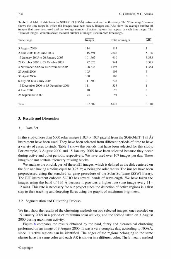
Table 1 A table of data from the SOHO/EIT (195Å) instrument used in this study. The ‘Time range’ columnshows the time range in which the images have been taken, Images and ARs show the average number ofimages that have been used and the average number of active regions that appear in each time range. The‘Total of images’ column shows the total number of images used in each time range.
Time range Images Total of images ARs
3 August 2000 114 114 11
2 June 2003 to 23 June 2003 115.591 2543 5.136
15 January 2005 to 20 January 2005 101.667 610 3.333
22 October 2005 to 29 October 2005 92.625 741 0.375
4 November 2005 to 14 November 2005 108.636 1195 1.364
27 April 2006 105 105 3
30 April 2006 100 100 3
6 July 2006 to 7 July 2006 111.500 223 2
13 December 2006 to 15 December 2006 111 333 1
4 June 2007 70 70 3
28 September 2009 94 94 2
Total 107.509 6128 3.140
3. Results and Discussion
3.1. Data Set
In this study, more than 6000 solar images (1024×1024 pixels) from the SOHO/EIT (195 Å)instrument have been used. They have been selected from different periods of time to havea variety of cases to study. Table 1 shows the periods that have been selected for this study.For example, 3 August 2000 and 15 January 2005 have been selected because they occurduring active and quiet periods, respectively. We have used over 107 images per day. Theseimages do not contain telemetry missing blocks.
We analyze the on-disk part of these EIT images, which is defined as the disk centered onthe Sun and having a radius equal to 0.95 R; R being the solar radius. The images have beenpreprocessed using the standard eit_prep procedure of the Solar Software (SSW) library.The EIT instrument onboard SOHO has several bands of wavelength. We have taken theimages using the band of 195 Å because it provides a higher rate (one image every 11 –12 min). This rate is necessary for our project since the detection of active regions is a firststep to then tracking and detecting flares using the graphs of maximum brightness.
3.2. Segmentation and Clustering Process
We first show the results of the clustering methods on two selected images: one recorded on15 January 2005 in a period of minimum solar activity, and the second taken on 3 August2000 during maximum activity.
Figure 8 compares the results obtained by the hard, fuzzy and hierarchical clusteringperformed on an image of 3 August 2000. It was a very complex day, according to NOAA,since 11 active regions can be identified. The edges of the regions belonging to the samecluster have the same color and each AR is shown in a different color. The k-means method

Clustering Methods for Active Region Detection in Solar EUV Images 707
Figure 8 (a) Original image from SOHO/EIT (195 Å) of August 2000. The rest of the panels are the resultsobtained using the c-means and the PC/PE indices, (b) k-means and the index of Chou (c), and AGNES andthe RMSSTD/RS indices (d).
using Chou’s validity index and the c-means method using the PC/PE validity indices identi-fied only two active regions. Furthermore, these two active regions do not correspond to anyactive region reported by NOAA. In contrast, the proposed hierarchical clustering methodobtained a satisfactory clustering because it identifies nine active regions, which correspondto active regions reported by NOAA.
Figure 9 compares the results obtained by the three clustering methods performed on animage taken on 15 January 2005. According to NOAA, on this day there were only twoactive regions but another unlabeled bright regions appears in the image. These bright re-gions were reported as AR by NOAA during the following days. The hierarchical clusteringmethod identifies four clusters. Two of them correspond to the ARs reported by NOAA thatday. In addition, another one corresponds to the bright region that was reported as an AR byNOAA on 16 January 2005. On the other hand, hard and fuzzy methods incorrectly identifythe active regions. The k-means method using Chou’s validity index identified only threeactive regions, because two active regions were merged into a single one. The c-means clus-tering method using the PC/PE validity indices identified only two clusters which do notcorrespond to any AR identified by NOAA.
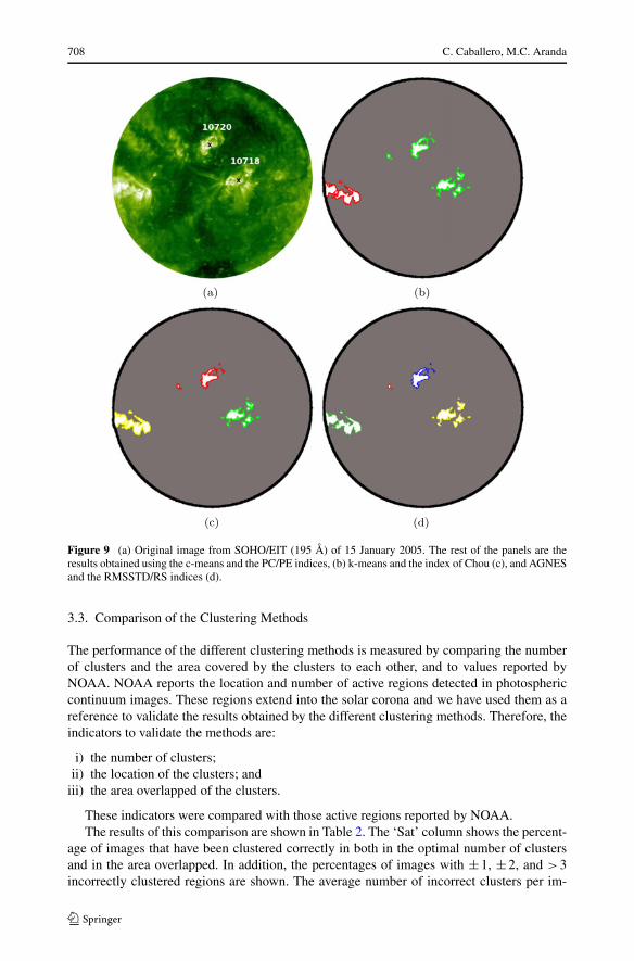
708 C. Caballero, M.C. Aranda
Figure 9 (a) Original image from SOHO/EIT (195 Å) of 15 January 2005. The rest of the panels are theresults obtained using the c-means and the PC/PE indices, (b) k-means and the index of Chou (c), and AGNESand the RMSSTD/RS indices (d).
3.3. Comparison of the Clustering Methods
The performance of the different clustering methods is measured by comparing the numberof clusters and the area covered by the clusters to each other, and to values reported byNOAA. NOAA reports the location and number of active regions detected in photosphericcontinuum images. These regions extend into the solar corona and we have used them as areference to validate the results obtained by the different clustering methods. Therefore, theindicators to validate the methods are:
i) the number of clusters;ii) the location of the clusters; and
iii) the area overlapped of the clusters.
These indicators were compared with those active regions reported by NOAA.The results of this comparison are shown in Table 2. The ‘Sat’ column shows the percent-
age of images that have been clustered correctly in both in the optimal number of clustersand in the area overlapped. In addition, the percentages of images with ±1, ±2, and >3incorrectly clustered regions are shown. The average number of incorrect clusters per im-
Clustering Methods for Active Region Detection in Solar EUV Images 709
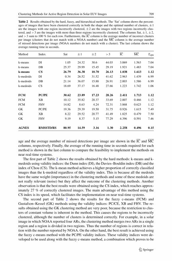
Table 2 Results obtained by the hard, fuzzy, and hierarchical methods. The ‘Sat’ column shows the percent-ages of images that have been clustered correctly in both the shape and the optimal number of clusters, ±1are the images with one region incorrectly clustered, ±2 are the images with two regions incorrectly clus-tered, and >3 are the images with more than three regions incorrectly clustered. The columns Sat, ±1, ±2,and >3 sum to 100 % for each row. Furthermore, the IC column is the average number of incorrect clustersper image (clusters that do not match with a NOAA number) and the MC column is the average numberof missed detections per image (NOAA numbers do not match with a cluster). The last column shows theaverage running time in seconds.
Method Index Sat ±1 ±2 >3 IC MC Tcpu
k-means DI 1.05 24.32 30.6 44.03 3.069 1.563 7.04
k-means DB 25.37 29.99 15.45 29.19 1.921 1.483 7.04
k-means CS 26.79 36.38 10.70 26.13 1.038 1.613 1.12
k-medoids DI 0.34 26.52 31.52 41.62 2.963 1.439 6.99
k-medoids DB 21.14 36.07 15.88 26.91 2.003 1.586 6.99
k-medoids CS 18.69 37.17 16.48 27.66 1.223 1.742 1.06
FCM PC/PE 30.62 23.89 17.23 28.26 2.411 1.713 1.12
FCM XB 10.12 35.82 20.37 33.69 2.007 0.466 1.12
FCM FHV 14.82 8.63 4.24 72.31 3.868 0.623 1.12
GK PC/PE 19.36 29.39 19.50 31.75 0.926 1.615 7.49
GK XB 8.22 29.52 20.77 41.49 1.825 0.479 7.50
GK FHV 9.19 8.37 5.15 77.29 4.396 0.591 7.46
AGNES RMSSTD/RS 80.95 14.59 3.16 1.30 2.258 0.496 0.15
age and the average number of missed detections per image are shown in the IC and MCcolumns, respectively. Finally, the average of the running time in seconds required for eachmethod is shown in the last column to compare the feasibility to implement the methods onnear real-time systems.
The first part of Table 2 shows the results obtained by the hard methods: k-means and k-medoids using validity indices: the Dunn index (DI), the Davies–Bouldin index (DB) and theindex of Chou (CS). The k-mean method achieves a higher proportion of correctly classifiedimages than the k-medoid regardless of the validity index. This is because all the medoidshave the same weight (importance) in the clustering methods and some of these medoids arenot really relevant (noise) but they affect the outcome of the clustering methods. Anotherobservation is that the best results were obtained using the CS index, which reaches approx-imately 27 % of correctly clustered images. The main advantage of this method using theCS index is its speed, which facilitates the implementation on near real-time systems.
The second part of Table 2 shows the results for the fuzzy c-means (FCM) andGustafson–Kessel (GK) methods using the validity indices: PC/CE, XB and FHV. The re-sults obtained using the GK clustering method are very poor, because the restriction to clus-ters of constant volume is inherent in the method. This causes the regions to be incorrectlyclustered, although the number of clusters is determined correctly. For example, in a solarimage in which NOAA reported four ARs, the clustering method merges two ARs in a singleregion and a region is divided in two regions. Thus the number of regions is correct in rela-tion with the number reported by NOAA. On the other hand, the best result is achieved usingthe fuzzy c-means method with the PC/PE validity indices. These validity indices were de-veloped to be used along with the fuzzy c-means method, a combination which proves to be
710 C. Caballero, M.C. Aranda
very satisfactory. Over 30 % of the images is clustered successfully using this method. Al-though the result is better than that achieved with hard methods, it is still too low to providerobustness.
Finally, the last row of Table 2 shows the results of a hierarchical method (AGNES) usingthe RMSSTD and RS validity indices and the best results achieved using fuzzy and hardmethods in bold text. It can be seen that the results achieved by the hierarchical method arebetter than those achieved by other proposed methods. Approximately 81 % of the imageswas successfully clustered using the hierarchical clustering method (AGNES) combinedwith the validity indices RMSSTD/RS. Furthermore, the percentage of images with ±1incorrectly clustered regions is 14.59 %. Another point of interest is the speed of the method,which means that it can be implemented in near real-time systems. The high speed of themethod is due to the characterization of the ROIs, which selects the points of the edge ofeach region (Section 2.2.1).
3.4. Stability of the System
This section presents the stability of the system in terms of the clustering of active regions,and then describes the main challenges to address:
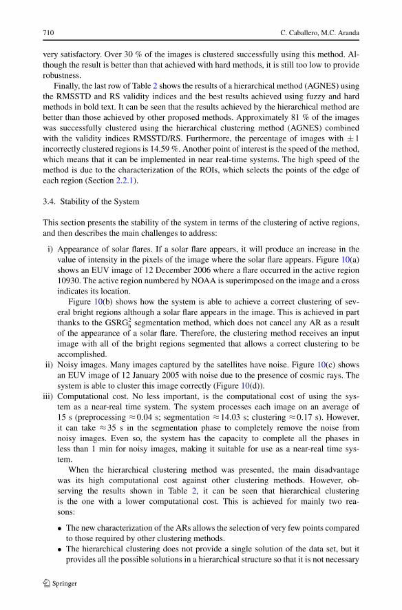
i) Appearance of solar flares. If a solar flare appears, it will produce an increase in thevalue of intensity in the pixels of the image where the solar flare appears. Figure 10(a)shows an EUV image of 12 December 2006 where a flare occurred in the active region10930. The active region numbered by NOAA is superimposed on the image and a crossindicates its location.
Figure 10(b) shows how the system is able to achieve a correct clustering of sev-eral bright regions although a solar flare appears in the image. This is achieved in partthanks to the GSRG2
h segmentation method, which does not cancel any AR as a resultof the appearance of a solar flare. Therefore, the clustering method receives an inputimage with all of the bright regions segmented that allows a correct clustering to beaccomplished.
ii) Noisy images. Many images captured by the satellites have noise. Figure 10(c) showsan EUV image of 12 January 2005 with noise due to the presence of cosmic rays. Thesystem is able to cluster this image correctly (Figure 10(d)).
iii) Computational cost. No less important, is the computational cost of using the sys-tem as a near-real time system. The system processes each image on an average of15 s (preprocessing ≈0.04 s; segmentation ≈14.03 s; clustering ≈0.17 s). However,it can take ≈35 s in the segmentation phase to completely remove the noise fromnoisy images. Even so, the system has the capacity to complete all the phases inless than 1 min for noisy images, making it suitable for use as a near-real time sys-tem.
When the hierarchical clustering method was presented, the main disadvantagewas its high computational cost against other clustering methods. However, ob-serving the results shown in Table 2, it can be seen that hierarchical clusteringis the one with a lower computational cost. This is achieved for mainly two rea-sons:
• The new characterization of the ARs allows the selection of very few points comparedto those required by other clustering methods.
• The hierarchical clustering does not provide a single solution of the data set, but itprovides all the possible solutions in a hierarchical structure so that it is not necessary

Clustering Methods for Active Region Detection in Solar EUV Images 711
Figure 10 (a) Unprocessed SOHO/EIT (195 Å) image of 12 December 2006 in which the AR numberedby NOAA is superimposed and a cross indicates its location. This image shows a solar flare in progress.(b) Resulting map of detections by our system using the image in panel (a) as input. The occurrence of thesolar flare has not affected the detections. (c) Unprocessed SOHO/EIT (195 Å) image of 18 January 2005 inwhich the ARs numbered by NOAA are superimposed on the image with crosses indicating their locations.This is a noisy image. (d) Resulting image after applying our system to original image (c) in which all thebright regions are identified without picking up noisy regions.
to recalculate the method iteratively for different configurations based on the numberof clusters.
3.5. Comparison Against Other Systems
This section presents a comparison of our system against other AR detection systems such asthe Spatial Possibilistic Clustering Algorithm (SPoCA) (Barra et al., 2009) and Solar Mon-itor Active Region Tracking (SMART) (Higgins et al., 2010). There are also other methodsfocussing on identifying and tracking sunspots, such as Automated Solar Activity Prediction(ASAP) (Colak and Qahwaji, 2009) and the Sunspot Tracking And Recognition Algorithm(STARA) (Watson et al., 2009). Our results have been compared with those by Verbeecket al. (2011).
SMART identifies features with a magnetic field strength above a certain threshold usingSOHO Michelson Doppler Imager (MDI; Scherrer et al., 1995) magnetograms that are later

712 C. Caballero, M.C. Aranda
Figure 11 Number of active regions detected by SMART, SPoCA, and our system compared with the onesreported by NOAA.
used for the identification of ARs. On the other hand, SPoCA uses images in EUV to detectARs in the solar corona. Since SPoCA is the more similar method to the one presented inthis paper, a more detailed comparison is made.
Figure 11 compares the daily number of regions detected by SMART, SPoCA and oursystem versus the daily number of regions reported by NOAA in a period of 23 days ofJune 2003. Note that our system obtains results closer to those reported by NOAA. Thereare some days in which our system identifies less regions than NOAA. This is because oursystem merges several regions into a single region. The regions that our system identifies asa single region are the regions that in the EUV band are difficult to separate because theyform a single bright region.
A more detailed comparison between SPoCA and our system is performed since bothsystems use information regarding the solar corona provided by images in EUV. The dataused for the comparison between SPoCA and our system are described in Verbeeck et al.(2011, Section 4.3.1). The first interesting point is that NOAA regions 10377 and 10375 aredetected as a single region by SPoCA for the period from 3 to 6 June and 11 June, whereasour system easily differentiates these two regions. These regions are clearly separated andthey do not appear as a single bright region in the solar corona. In addition, Figure 11 showsthat SPoCA detects a greater number of ARs than those identified by NOAA. This meansthat, although SPoCA identifies a greater number of ARs, these are not the same as NOAAreports.
Secondly, on some days our system identifies less regions than those identified by NOAA.It is because the magnetic foot points of these regions are very close together and thereforethe images in the EUV band appear as a single bright region. However, regions 10377 and10375 are identified by our system since they are well separated.

Clustering Methods for Active Region Detection in Solar EUV Images 713
4. Conclusions
This paper has presented a comparative study of different clustering methods and validityindices applied to the detection of solar active regions. The results have been very posi-tive, because the active regions matched NOAA in approximately 81 % of cases using thehierarchical clustering method (AGNES) combined with the validity indices RMSSTD/RS.
The segmentation of solar images was performed using the GSRG2h method. It has two
major advantages since it is stable in images with large differences in brightness (such asimages with a flare) and also it is stable in noisy images (the noise does not affect thesegmentation).
Clustering methods have been used to group together previously segmented regions toform consistent active regions. Hierarchical methods have been found to be best suited tosolve this problem, as well as a viable solution for near real-time systems due to the char-acterization of the problem that has been proposed. This characterization involves takingthe edge points of the segmented regions as input to clustering methods instead of select-ing a single value per region (medoid-means techniques) or all points in the region (densitytechniques).
The study uses a database of over 6000 solar images from SOHO/EIT (195 Å). The ac-tive regions obtained from the clustering method are compared with those active regionsobtained by NOAA. Moreover, images incorrectly clustered using the hierarchical cluster-ing method could be interpreted correctly in a post-clustering procedure using AR trackingmethods.
The formation of these groups facilitates the subsequent monitoring of these regions.Flares can also be detected and assigned to a specific region by using graphs of maximumbrightness of each region. A catalogue of ARs describing key parameters, such as theirlocation, shape, area, and mean and integrated intensities could be created to relate thoseproperties to the occurrence of flares.
Acknowledgements This work was funded by the project TIC07-02861 of the Junta de Andalucía (Spain).
Appendix A: GSRG2h: Seed Selection
In the GSRG2h method, seed selection is carried out using a histogram-based technique.
In particular, it uses the histogram shape of the solar images after preprocessing. In thepreprocessed solar images, most pixels have a value close to zero, so that pixels with thehighest values of the histogram have few occurrences.
The threshold that determines the value of the seeds is calculated using the points of thehistogram. The histogram of preprocessed solar images decreases and therefore the straightline that represents these points has a decreasing slope. If the threshold value is determinedat the beginning of the fall of the histogram, then the level of intensity of the pixels thatare selected will be too low. This means that irrelevant pixels (noise) are taken as relevantobjects. On the other hand, if the threshold value is determined at the end of the fall of thehistogram, then relevant objects are taken as noise. Therefore, the ideal threshold is close tothe beginning of the fall, but not just at the beginning.
Let fi be the function that performs a least-square linear fit to the points of the histogramand let ai be the slope of the function fi . Furthermore, let FC be the family of functionsfi whose slope satisfies the condition ai < σc , where the threshold σc is defined with a

714 C. Caballero, M.C. Aranda
Algorithm 1: GSRG2h: Seed Selection
Input: I : Preprocessed solar image.Output: seeds: Set of seeds to be used with the SRG method.Data: FC = ∅, P = ∅, σc = positive small value, σp = negative small value, �c = an
increasing factor, �p = an increasing factor.The functions fi and its slope ai are calculated1
while size(FC) = 0 do2
foreach fi do3
if ai < σc then4
FC.add(fi)5
σc = σc · �c6
The functions gi and its slope ci are calculated7
while size(P ) = 0 do8
foreach fi do9
if FC.contains(fi) and ci > σp then10
P.add(fi)11
σp = σp · �p12
seeds = I (x, y) < round(P .first().getX())13
very small value. If any function fi satisfies the previous condition, then the threshold σc ismodified by an increasing factor (�c).
The family of functions gi are also calculated, where the histogram points used to calcu-late the functions gi are the following histogram points that have been used to calculate thefunctions fi . The family of functions gi are used to determine the trend of the points aftereach of the pre-selected functions fi . Therefore, the threshold σp is defined as a negativevalue and small enough to consider those functions with a small slope and discard thosefunctions with a large fall, which are often the first.
Finally, let P be the family of functions fi of the set FC that also satisfy the conditionci < σp where ci is defined as the slope of the function gi . If any function fi satisfies theprevious conditions then the threshold σp is modified using an increasing factor (�p). Thevalue of the threshold is determined by the average of the values xj and xk from the firstpoint (xj , xk) of the set P . The first point of the set P is selected because this point has thesmallest values of xj and xk .
Appendix B: Seeded Region Growing
In this appendix the pseudocode of the seeded region growing (SRG) algorithm is presented,which is described in detail in Adams and Bischof (1994).

Clustering Methods for Active Region Detection in Solar EUV Images 715
Algorithm 2: Seeded region growing
Data: A sequentially sorted list (SSL) which contains the elements of the set T isdefined
The GSRG2h seed selection method is applied to initialize the set T .1
while not(isempty(SSL)) do2
Delete the first pixel y of SSL.3
Check the neighbors of the pixel y.4
if All the neighbors of the pixel y are assigned to the same region then5
Assign the region to the pixel y. Update the average values of the region to6
which the pixel is assigned.Add to the list SSL neighbors of the pixel y that were not already assigned to a7
region and that were not already on the list SSL.
else8
The value of the edge is assigned to the pixel y.9
References
Aboudarham, J., Scholl, I., Fuller, N., Fouesneau, M., Galametz, M., Gonon, F., Maire, A., Leroy, Y.: 2008,Automatic detection and tracking of filaments for a solar feature database. Ann. Geophys. 26, 243 – 248.
Adams, R., Bischof, L.: 1994, Seeded region growing. IEEE Trans. Pattern Anal. Mach. Intell. 16, 641 – 647.Alonso Moral, J.M.: 2007, Interpretable fuzzy systems modeling with cooperation between expert and in-
duced knowledge. Ph.D. thesis, Universidad Politécnica de Madrid.Anderberg, M.: 1973, Cluster Analysis for Applications, Academic Press, New York, 395.Aranda, M.C., Caballero, C.: 2010, Automatic detection of active region on EUV solar images using
fuzzy clustering. In: Hüllermeier, E., Kruse, R., Hoffmann, F. (eds.) Computational Intelligence forKnowledge-Based Systems Design, Lecture Notes in Computer Science 6178, Springer, Berlin, 69 – 78.
Arthur, D., Vassilvitskii, S.: 2007, k-means++: the advantages of careful seeding. In: Gabow, H. (ed.) Pro-ceedings of the Eighteenth Annual ACM-SIAM Symposium on Discrete Algorithms, Society for Indus-trial and Applied Mathematics, Philadelphia, 1027 – 1035.
Babuska, R., der Venn, P.J.V., Kaymak, U.: 2002, Improved variance estimation for Gustafson Kessel clus-tering. In: Proceedings of the 2002 IEEE International Conference on Fuzzy Systems, 1081 – 1085.
Barra, V., Delouille, V., Hochedez, J.-F.: 2008, Segmentation of extreme ultraviolet solar images via multi-channel fuzzy clustering. Adv. Space Res. 42, 917 – 925.
Barra, V., Delouille, V., Kretzschmar, M., Hochedez, J.F.: 2009, Fast and robust segmentation of solar EUVimages: Algorithm and results for solar cycle 23. Astron. Astrophys. 505, 361 – 371.
Benkhalil, A., Zharkova, V., Ipson, S., Zharkov, S.: 2006, Active region detection and verification with thesolar feature catalogue. Solar Phys. 235, 87 – 106.
Bezdek, J.C.: 1981, Pattern Recognition with Fuzzy Objective Function Algorithms, Plenum Press, New York,256.
Bezdek, J.C., Dunn, J.C.: 1975, Optimal fuzzy partitions: A heuristic for estimating the parameters in amixture of normal distribution. IEEE Trans. Comput. 24, 835 – 838.
Bezdek, J.C., Ehrlich, R., Full, W.: 1984, FCM: Fuzzy c-means algorithm. Comput. Geosci. 10, 191 – 203.Chou, C., Su, M., Lai, E.: 2004, A new cluster validity measure and its application to image compression.
Pattern Anal. Appl. 7, 205 – 220.Colak, T., Qahwaji, R.: 2008, Automated McIntosh-based classification of sunspot groups using MDI images.
Solar Phys. 248, 277 – 296.Colak, T., Qahwaji, R.: 2009, Automated solar activity prediction: A hybrid computer platform using machine
learning and solar imaging for automated prediction of solar flares. Space Weather 7, S06001.Davies, D.L., Bouldin, D.W.: 1979, A cluster separation measure. IEEE Trans. Pattern Anal. Mach. Intell. 1,
224 – 227.Delaboudiniére, J.-P., Artzner, G.E., Brunaud, J., Gabriel, A.H., Hochedez, J.F., Millier, F., et al.: 1995, EIT:
Extreme-ultraviolet Imaging Telescope for the SOHO mission. Solar Phys. 162, 291 – 312.Dunn, J.C.: 1974, Well-separated clusters and optimal fuzzy partitions. J. Cybern. 4, 95 – 104.
716 C. Caballero, M.C. Aranda
Fukuyama, Y., Sugeno, M.: 1989, A new method of choosing the number of clusters for the fuzzy c-meansmethod. In: Proceedings of Fifth Fuzzy System Symposium, 247 – 250.
Fuller, N., Aboudarham, J., Bentley, R.: 2005, Filament recognition and image cleaning on Meudon Hαspectroheliograms. Solar Phys. 227, 61 – 73.
Gath, I., Geva, A.B.: 1989, Unsupervised optimal fuzzy clustering. IEEE Trans. Pattern Anal. Mach. Intell.11, 773 – 781.
Ghaemi, R., Sulaiman, N., Ibrahim, H., Mustapha, N.: 2009, A survey: Clustering ensembles techniques.Proc. World Acad. Sci., Eng. Technol. 38, 644 – 653.
Gustafson, D.E., Kessel, W.C.: 1978, Fuzzy clustering with a fuzzy covariance matrix. In: IEEE Conferenceon Decision and Control including the 17th Symposium on Adaptive Processes, 761 – 766.
Halkidi, M., Batistakis, Y., Varzigiannis, M.: 2002a, Cluster validity methods part I. ACM SIGMOD Rec. 31,40 – 45.
Halkidi, M., Batistakis, Y., Varzigiannis, M.: 2002b, Cluster validity methods part II. ACM SIGMOD Rec. 31,19 – 27.
Hartigan, J.: 1975, Clustering Algorithms, Wiley, New York, 351.Higgins, P., Gallagher, P., McAteer, R., Bloomfield, D.: 2010, Solar magnetic feature detection and tracking
for space weather monitoring. Adv. Space Res. 47, 2105 – 2117.Jain, A., Dubes, R.: 1988, Algorithms for Clustering Data, Prentice Hall, Englewood Cliffs, 320.Joshi, A., Srivastava, N., Mathew, S.: 2010, Automated detection of filaments and their disappearance using
full-disc Hα images. Solar Phys. 262, 425 – 436.Kaufman, L., Rousseeuw, P.J.: 1987, Clustering by means of medois. Technical Report, Vrije Universiteit.Kaufman, L., Rousseeuw, P.J.: 1990, Finding Groups in Data: An Introduction to Cluster Analysis, Wiley-
Interscience, New York, 342.Krista, L., Gallagher, P.: 2009, Automated coronal hole detection using local intensity thresholding tech-
niques. Solar Phys. 256, 87 – 100.Macqueen, J.B.: 1967, Some methods for classification and analysis of multivariate observations. In: Le Cam,
L.M., Neyman, J. (eds.) Proc. Fifth Berkeley Symp. Mathematical Statistics and Probability 1, Univ.California Press, Berkeley, 281 – 297.
McAteer, R., Gallagher, P., Ireland, J., Young, C.: 2005, Automated boundary-extraction and region-growingtechniques applied to solar magnetograms. Solar Phys. 228, 55 – 66.
Nguyen, T., Willis, C., Paddon, D., Nguyen, H.: 2006, A hybrid system for learning sunspot recognition andclassification. In: Proceedings of the 2006 International Conference on Hybrid Information Technology2, Washington, 257 – 264.
Nieniewski, M.: 2004, Extraction of diffuse objects from images by means of watershed and region merging:example of solar images. IEEE Trans. Syst. Man Cybern., Part B, Cybern. 34, 796 – 801.
Otsu, N.: 1979, A threshold selection method from grey level histograms. IEEE Trans. Syst. Man Cybern. 9,62 – 66.
Pesnel, W.D., Thompson, B.J., Chamberlin, P.C.: 2012, The solar dynamics observatory (SDO). Solar Phys.275, 3 – 15.
Qahwaji, R., Colak, T.: 2006, Automatic detection and verification of solar features. Int. J. Imaging Syst.Technol. 4, 199 – 210.
Ridpath, I.: 2012, A Dictionary of Astronomy, 2nd edn., Oxford Univ. Press, New York.Robbrecht, E., Berghmans, D., van der Linden, R.: 2006, Objective CME detection over the solar cycle:
A first attempt. Adv. Space Res. 38, 475 – 479.Scherrer, P.H., Bogart, R.S., Bush, R.I., Hoeksema, J.T., Kosovichev, A.G., Schou, J., et al.: 1995, The Solar
Oscillation Investigation – Michelson-Doppler Imager. Solar Phys. 162, 129 – 188.Sharma, S.: 1996, Applied Multivariate Techniques, Wiley, New York, 225.Steinhaus, H.: 1956, Sur la division des corp materiels en parties. Bull. Acad. Pol. Sci 1, 801 – 804.Sych, R., Nakariakov, V., Karlicky, M., Afinogentov, S.: 2009, Relationship between wave processes in
sunspots and quasi-periodic pulsations in active region flares. Astron. Astrophys. 505, 791 – 799.Tibshirani, R., Walter, G., Hastie, T.: 2001, Estimating the number of cluster in a dataset via the gap statistic.
J. Roy. Stat. Soc. B 32, 411 – 423.Verbeeck, C., Higgins, T., Colak, T., Watson, T., Delouille, V., Mapaey, B., Qahwaji, R.: 2011, A multi-
wavelength analysis of active regions and sunspots by comparison of automatic detection algorithms.Solar Phys. 283, 67–95.
Veronig, A., Steinegger, M., Otruba, W., Hanslmeier, A., Messerotti, M., Temmer, M., Gonzi, S., Brunner,G.: 2000, Automatic image processing in the frame of a solar flare alerting system. Hvar Obs. Bull. 24,195 – 205.
Watson, F., Fletcher, L., Dalla, S., Marshall, S.: 2009, Modelling the longitudinal asymmetry in sunspotemergence: The role of the Wilson depression. Solar Phys. 260, 5 – 19.

Clustering Methods for Active Region Detection in Solar EUV Images 717
Wu, K.-L., Yang, M.-S.: 2005, A cluster validity index for fuzzy clustering. Pattern Recognit. Lett. 26, 1275 –1291.
Xie, X.L., Beni, G.: 1991, A validity measure for fuzzy clustering. IEEE Trans. Pattern Anal. Mach. Intell.13, 841 – 846.
Xu, R., Wunsch, D.: 2008, Clustering, Wiley-IEEE Press, New York, 368.Yeung, K.Y., Haynor, D.R., Ruzzo, W.L.: 2001, Validating clustering for gene expression data. Bioinformatics
17, 309 – 318.Young, C., Gallagher, P.: 2008, Multiscale edge detection in the corona. Solar Phys. 248, 457 – 469.Zharkov, S., Zharkova, V.: 2011, Statistical properties of Hα flares in relation to sunspots and active regions
in the cycle 23. J. Atmos. Solar-Terr. Phys. 73, 264 – 270.Zharkov, S., Zharkova, V., Ipson, S., Benkhalil, A.: 2004, Automated recognition of sunspots on the
SOHO/MDI white light solar images. In: Negoita, M.G., Howlett, R.J., Jain, L.C. (eds.) Knowledge-Based Intelligent Information and Engineering Systems, Springer, Berlin, 446 – 452.