5 5 production, inputs, and cost: building blocks for supply analysis
Post on 22-Dec-2015
221 views
TRANSCRIPT
5
Production, Inputs, and Cost: Building Blocks for
Supply Analysis
Copyright© 2006 South-Western/Thomson Learning. All rights reserved.
● Production and Input Choice, with One Variable Input
● Multiple Input Decisions: The Choice of Optimal Input Combinations
● Cost and Its Dependence on Output
● Economies of Scale
● Production and Input Choice, with One Variable Input
● Multiple Input Decisions: The Choice of Optimal Input Combinations
● Cost and Its Dependence on Output
● Economies of Scale
OutlineOutline
Copyright© 2006 South-Western/Thomson Publishing. All rights reserved.
Copyright© 2006 South-Western/Thomson Learning. All rights reserved.
Production and Input Choice, with 1 Variable InputProduction and Input Choice, with 1 Variable Input
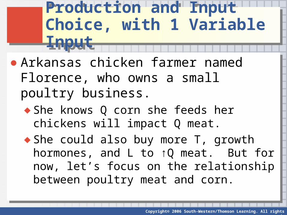
● Arkansas chicken farmer named Florence, who owns a small poultry business. ♦ She knows Q corn she feeds her chickens will impact
Q meat. ♦ She could also buy more T, growth hormones, and L
to ↑Q meat. But for now, let’s focus on the relationship between poultry meat and corn.
● Arkansas chicken farmer named Florence, who owns a small poultry business. ♦ She knows Q corn she feeds her chickens will impact
Q meat. ♦ She could also buy more T, growth hormones, and L
to ↑Q meat. But for now, let’s focus on the relationship between poultry meat and corn.
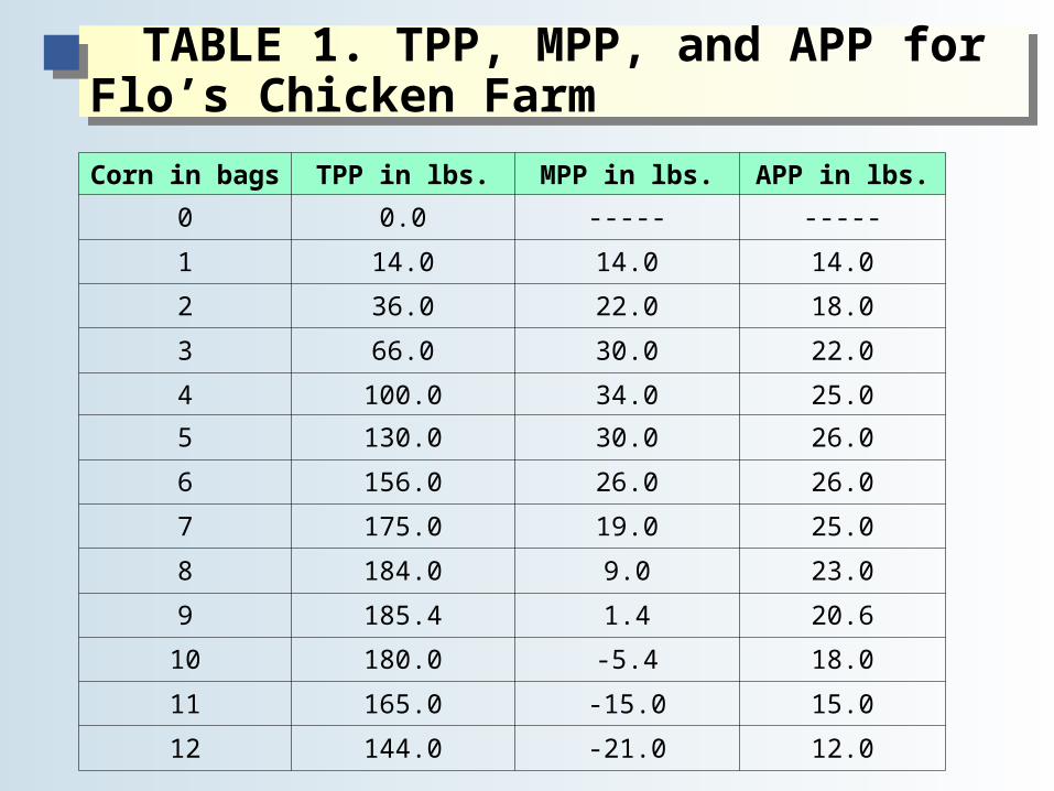
TABLE 1. TPP, MPP, and APP for Flo’s Chicken Farm
TABLE 1. TPP, MPP, and APP for Flo’s Chicken Farm
Corn in bags TPP in lbs. MPP in lbs. APP in lbs.
0 0.0 ----- -----
1 14.0 14.0 14.0
2 36.0 22.0 18.0
3 66.0 30.0 22.0
4 100.0 34.0 25.0
5 130.0 30.0 26.0
6 156.0 26.0 26.0
7 175.0 19.0 25.0
8 184.0 9.0 23.0
9 185.4 1.4 20.6
10 180.0 -5.4 18.0
11 165.0 -15.0 15.0
12 144.0 -21.0 12.0
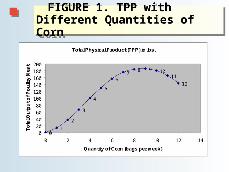
FIGURE 1. TPP with Different Quantities of Corn
FIGURE 1. TPP with Different Quantities of Corn
Total Physical Product (TPP) in lbs.
01
2
3
4
5
67
8 9 1011
12
020406080
100120140160180200
0 2 4 6 8 10 12 14
Quantity of Corn (bags per week)
To
tal O
utp
ut
of
Po
ult
ry M
ea
t

Copyright© 2006 South-Western/Thomson Learning. All rights reserved.
Production and Input Choice, with 1 Variable InputProduction and Input Choice, with 1 Variable Input
● Total Physical Product (TPP) = amount of output that can be produced as 1 input changes, with all other inputs held constant.♦ Table 1 shows TPP or how much chicken Flo can
produce with different Q corn, holding all other inputs fixed.
♦ If Q corn = 0 → Q meat = 0. Each add. bag of corn yields more poultry. 4 bags → 100 lbs. After 9 bags, ↑corn → ↓output –chickens are so overfed they become ill.

Copyright© 2006 South-Western/Thomson Learning. All rights reserved.
Production and Input Choice, with 1 Variable InputProduction and Input Choice, with 1 Variable Input
● Average physical product (APP) = TPP/(Q of input) = measures output per unit of input. ♦ E.g., 4 bags corn → 100 lbs meat, so APP = 25.
● Marginal physical product (MPP) = additional output resulting from a 1 unit increase in the
input, holding all other inputs constant. ♦ E.g., ↑corn from 4 to 5 bags, the 5th bag yields an
add. 30 lbs of meat.

FIGURE 2. Flo’s MPP Curve FIGURE 2. Flo’s MPP Curve
MPP
Bags of corn
00
9
14
34
4 120
-21
NegativeFallingRising
MPP
Copyright© 2006 South-Western/Thomson Learning. All rights reserved.
Graph of MPPGraph of MPP
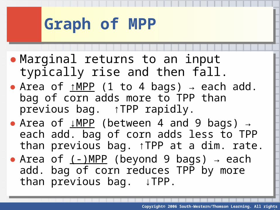
● Marginal returns to an input typically rise and then fall.
● Area of ↑MPP (1 to 4 bags) → each add. bag of corn adds more to TPP than previous bag. ↑TPP rapidly.
● Area of ↓MPP (between 4 and 9 bags) → each add. bag of corn adds less to TPP than previous bag. ↑TPP at a dim. rate.
● Area of (-)MPP (beyond 9 bags) → each add. bag of corn reduces TPP by more than previous bag. ↓TPP.
Copyright© 2006 South-Western/Thomson Learning. All rights reserved.
● ↑ Q of any one input, holding Q of all other inputs constant, leads to lower marginal returns to the expanding input.♦ E.g., Flo feeds chickens more and more, without
giving them extra water, cleaning up after them more, or buying add. chickens. Eventually overfed and become sick.
● Law of dim. marginal returns should hold for most activities.
Can you think of one?
The “Law” of Diminishing Marginal Returns The “Law” of Diminishing Marginal Returns
Copyright© 2006 South-Western/Thomson Publishing. All rights reserved.
Copyright© 2006 South-Western/Thomson Learning. All rights reserved.
Optimal Purchase Rule for a Single InputOptimal Purchase Rule for a Single Input
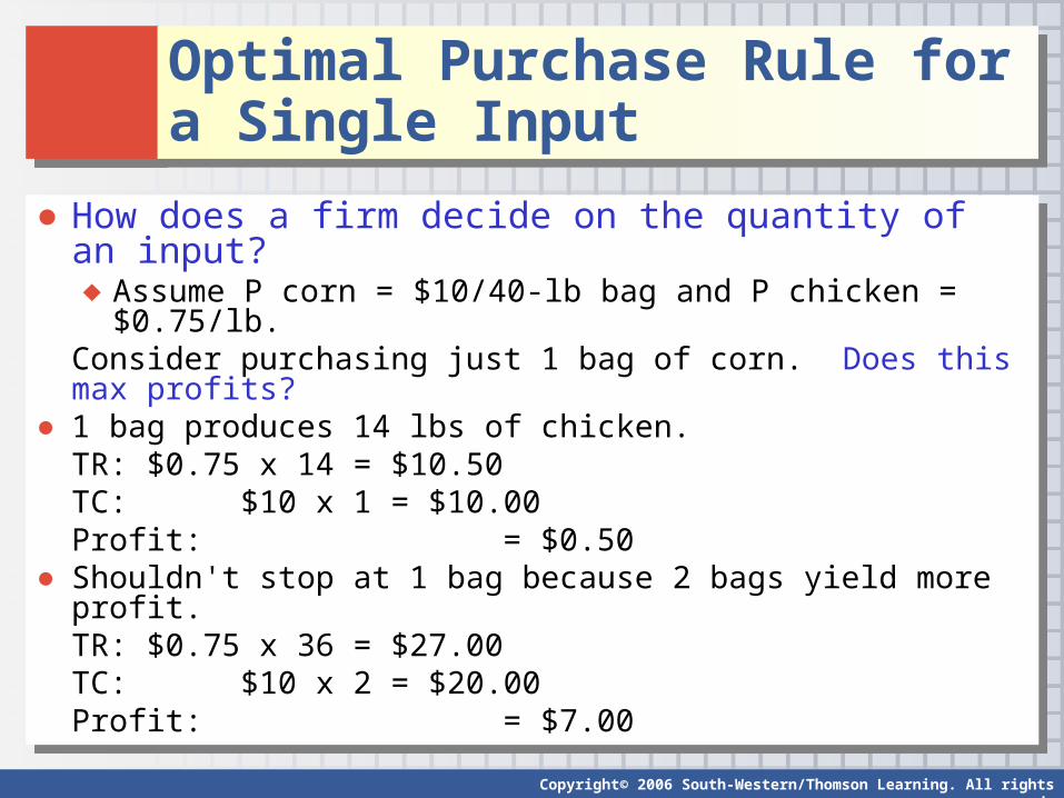
● How does a firm decide on the quantity of an input?♦ Assume P corn = $10/40-lb bag and P chicken = $0.75/lb.
Consider purchasing just 1 bag of corn. Does this max profits?● 1 bag produces 14 lbs of chicken.
TR: $0.75 x 14 = $10.50TC: $10 x 1 = $10.00Profit: = $0.50
● Shouldn't stop at 1 bag because 2 bags yield more profit.TR: $0.75 x 36 = $27.00TC: $10 x 2 = $20.00Profit: = $7.00
Copyright© 2006 South-Western/Thomson Learning. All rights reserved.
Optimal Purchase Rule for a Single InputOptimal Purchase Rule for a Single Input
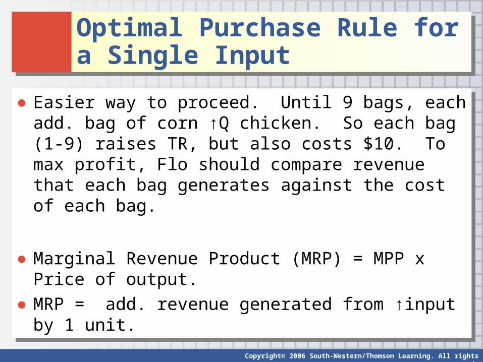
● Easier way to proceed. Until 9 bags, each add. bag of corn ↑Q chicken. So each bag (1-9) raises TR, but also costs $10. To max profit, Flo should compare revenue that each bag generates against the cost of each bag.
● Marginal Revenue Product (MRP) = MPP x Price of output.
● MRP = add. revenue generated from ↑input by 1 unit.
Bags ofCorn
TPP MPP TR(P*TPP)
MRP(P*MPP)
P corn Profit
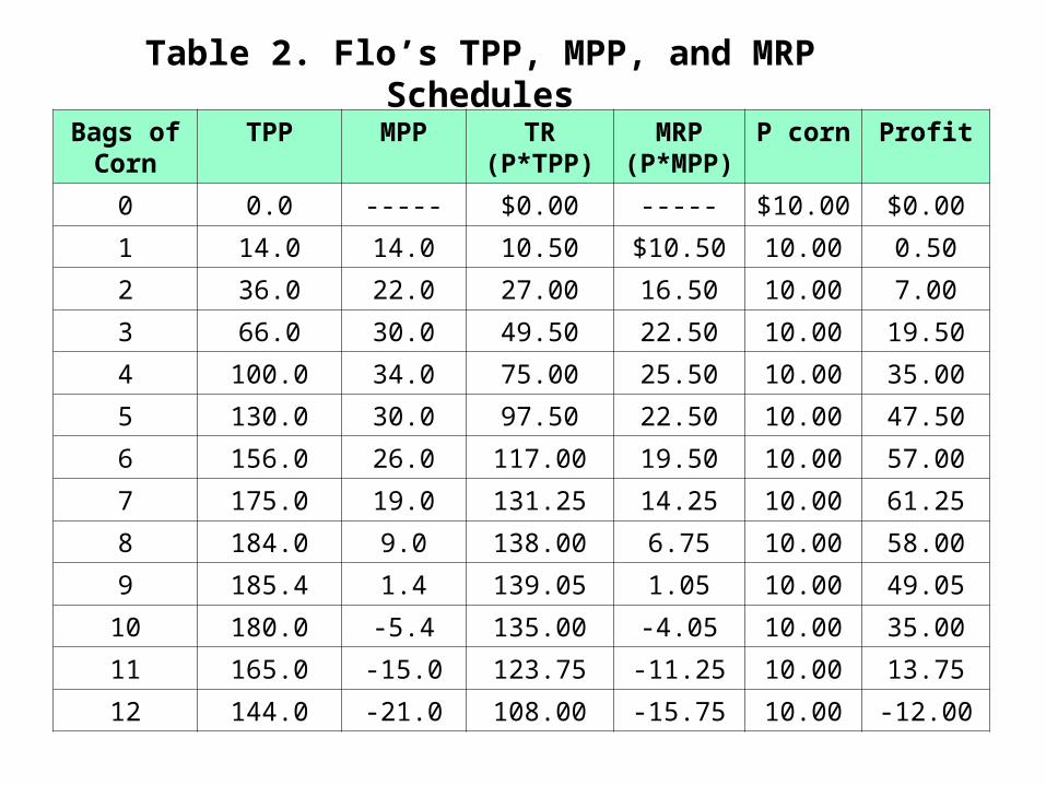
0 0.0 ----- $0.00 ----- $10.00 $0.00
1 14.0 14.0 10.50 $10.50 10.00 0.50
2 36.0 22.0 27.00 16.50 10.00 7.00
3 66.0 30.0 49.50 22.50 10.00 19.50
4 100.0 34.0 75.00 25.50 10.00 35.00
5 130.0 30.0 97.50 22.50 10.00 47.50
6 156.0 26.0 117.00 19.50 10.00 57.00
7 175.0 19.0 131.25 14.25 10.00 61.25
8 184.0 9.0 138.00 6.75 10.00 58.00
9 185.4 1.4 139.05 1.05 10.00 49.05
10 180.0 -5.4 135.00 -4.05 10.00 35.00
11 165.0 -15.0 123.75 -11.25 10.00 13.75
12 144.0 -21.0 108.00 -15.75 10.00 -12.00
Table 2. Flo’s TPP, MPP, and MRP Schedules
Copyright© 2006 South-Western/Thomson Learning. All rights reserved.
Optimal Purchase Rule for a Single InputOptimal Purchase Rule for a Single Input
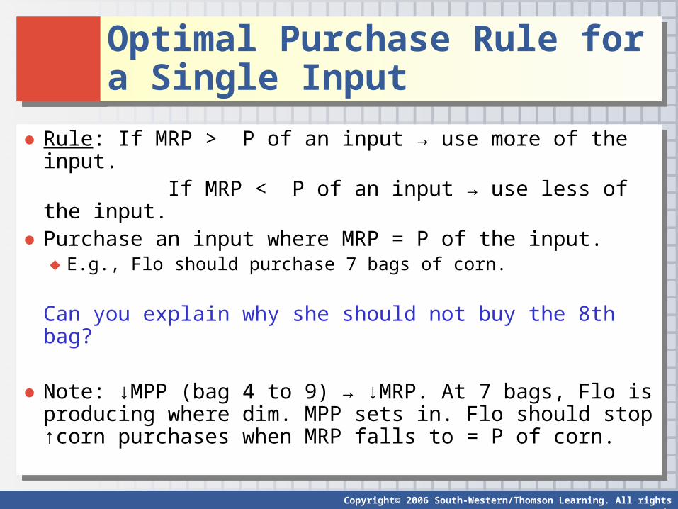
● Rule: If MRP > P of an input → use more of the input. If MRP < P of an input → use less of the input.
● Purchase an input where MRP = P of the input.♦ E.g., Flo should purchase 7 bags of corn.
Can you explain why she should not buy the 8th bag?
● Note: ↓MPP (bag 4 to 9) → ↓MRP. At 7 bags, Flo is producing where dim. MPP sets in. Flo should stop ↑corn purchases when MRP falls to = P of corn.
Copyright© 2006 South-Western/Thomson Learning. All rights reserved.
Multiple Input DecisionsMultiple Input Decisions
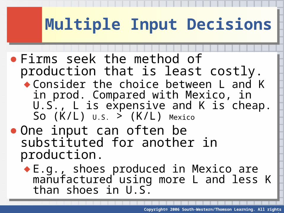
● Firms seek the method of production that is least costly.♦ Consider the choice between L and K in prod.
Compared with Mexico, in U.S., L is expensive and K is cheap. So (K/L) U.S. > (K/L) Mexico
● One input can often be substituted for another in production. ♦ E.g., shoes produced in Mexico are manufactured
using more L and less K than shoes in U.S.
Copyright© 2006 South-Western/Thomson Learning. All rights reserved.
Multiple Input DecisionsMultiple Input Decisions
● A firm can produce same amount of a good with less of one input (say L) as long as it’s willing to use more of another input (like K).
● Actual combos of inputs (such as K and L) depend on relative P of inputs. Firms strive to produce a good using the least expensive method.
● A firm can produce same amount of a good with less of one input (say L) as long as it’s willing to use more of another input (like K).
● Actual combos of inputs (such as K and L) depend on relative P of inputs. Firms strive to produce a good using the least expensive method.
Copyright© 2006 South-Western/Thomson Learning. All rights reserved.
Marginal Rule for Optimal Input ProportionsMarginal Rule for Optimal Input Proportions
● E.g., Flo can feed chickens soymeal or cornmeal –they are substitutes in production. ♦ Not perfect substitutes. Soymeal has more protein but
fewer carbohydrates than corn. ♦ Best to feed some combo of 2 meals. ↓Q poultry if Flo
relies too much on 1 input. There are dim. returns to substitution among the inputs.
Copyright© 2006 South-Western/Thomson Learning. All rights reserved.
Marginal Rule for Optimal Input ProportionsMarginal Rule for Optimal Input Proportions
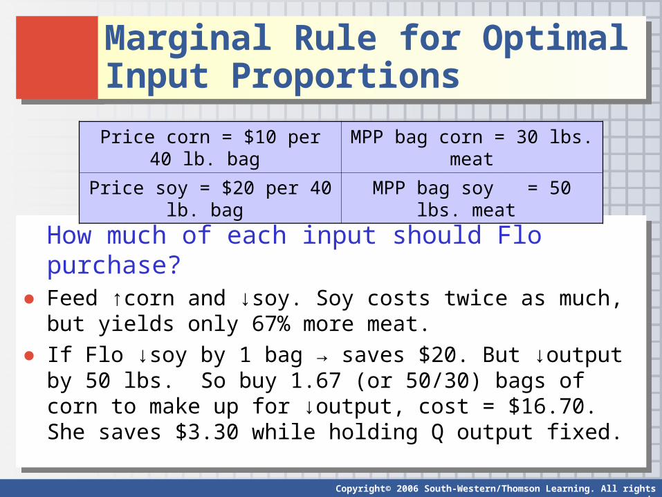
How much of each input should Flo purchase?● Feed ↑corn and ↓soy. Soy costs twice as much, but yields only
67% more meat.
● If Flo ↓soy by 1 bag → saves $20. But ↓output by 50 lbs. So buy 1.67 (or 50/30) bags of corn to make up for ↓output, cost = $16.70. She saves $3.30 while holding Q output fixed.
Price corn = $10 per 40 lb. bag MPP bag corn = 30 lbs. meat
Price soy = $20 per 40 lb. bag MPP bag soy = 50 lbs. meat
Copyright© 2006 South-Western/Thomson Learning. All rights reserved.
Marginal Rule for Optimal Input ProportionsMarginal Rule for Optimal Input Proportions
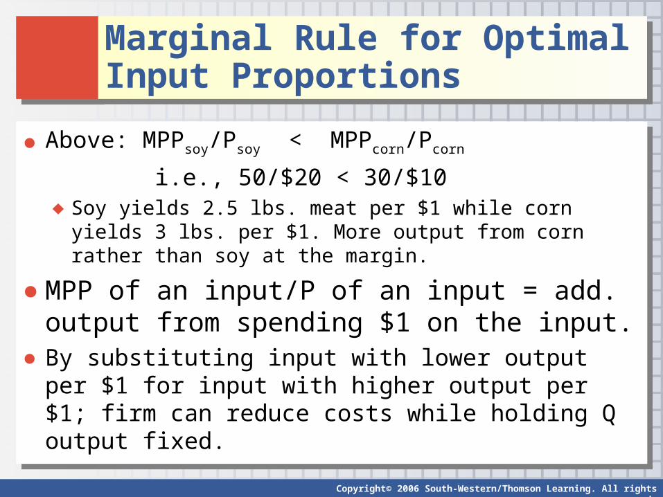
● Above: MPPsoy/Psoy < MPPcorn/Pcorn
i.e., 50/$20 < 30/$10♦ Soy yields 2.5 lbs. meat per $1 while corn yields 3 lbs. per $1.
More output from corn rather than soy at the margin.
● MPP of an input/P of an input = add. output from spending $1 on the input.
● By substituting input with lower output per $1 for input with higher output per $1; firm can reduce costs while holding Q output fixed.
Copyright© 2006 South-Western/Thomson Learning. All rights reserved.
Marginal Rule for Optimal Input ProportionsMarginal Rule for Optimal Input Proportions
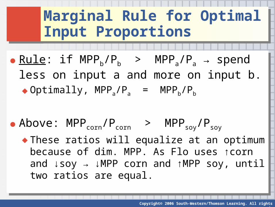
● Rule: if MPPb/Pb > MPPa/Pa → spend less on input a and more on input b.♦ Optimally, MPPa/Pa = MPPb/Pb
● Above: MPPcorn/Pcorn > MPPsoy/Psoy
♦ These ratios will equalize at an optimum because of dim. MPP. As Flo uses ↑corn and ↓soy → ↓MPP corn and ↑MPP soy, until two ratios are equal.
● Rule: if MPPb/Pb > MPPa/Pa → spend less on input a and more on input b.♦ Optimally, MPPa/Pa = MPPb/Pb
● Above: MPPcorn/Pcorn > MPPsoy/Psoy
♦ These ratios will equalize at an optimum because of dim. MPP. As Flo uses ↑corn and ↓soy → ↓MPP corn and ↑MPP soy, until two ratios are equal.
Copyright© 2006 South-Western/Thomson Learning. All rights reserved.
Marginal Rule for Optimal Input ProportionsMarginal Rule for Optimal Input Proportions
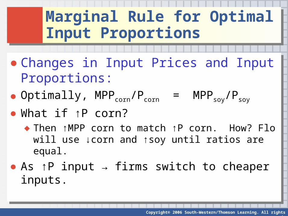
● Changes in Input Prices and Input Proportions:● Optimally, MPPcorn/Pcorn = MPPsoy/Psoy
● What if ↑P corn? ♦ Then ↑MPP corn to match ↑P corn. How? Flo will use ↓corn
and ↑soy until ratios are equal.
● As ↑P input → firms switch to cheaper inputs.
● Changes in Input Prices and Input Proportions:● Optimally, MPPcorn/Pcorn = MPPsoy/Psoy
● What if ↑P corn? ♦ Then ↑MPP corn to match ↑P corn. How? Flo will use ↓corn
and ↑soy until ratios are equal.
● As ↑P input → firms switch to cheaper inputs.

Copyright© 2006 South-Western/Thomson Learning. All rights reserved.
● 3 different cost curves –Total Cost (TC), Average Cost (AC), and Marginal Cost (MC).
● Flo’s costs depend on Q of inputs and on P of those inputs.
● To calculate costs, assume:♦ P corn is beyond Flo's control.♦ Q of all other inputs (except corn) are fixed.♦ P corn = $10 per 40 lb. bag
● 3 different cost curves –Total Cost (TC), Average Cost (AC), and Marginal Cost (MC).
● Flo’s costs depend on Q of inputs and on P of those inputs.
● To calculate costs, assume:♦ P corn is beyond Flo's control.♦ Q of all other inputs (except corn) are fixed.♦ P corn = $10 per 40 lb. bag
Cost Curves and Input QuantitiesCost Curves and Input Quantities
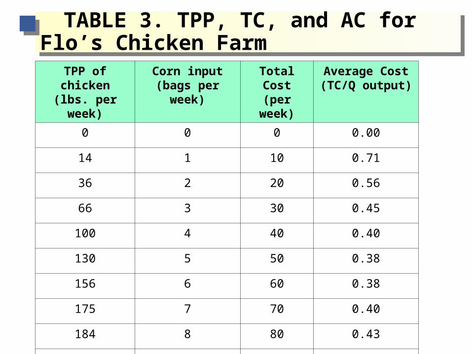
TABLE 3. TPP, TC, and AC for Flo’s Chicken Farm
TABLE 3. TPP, TC, and AC for Flo’s Chicken FarmTPP of chicken(lbs. per week)
Corn input(bags per week)
Total Cost(per week)
Average Cost(TC/Q output)
0 0 0 0.00
14 1 10 0.71
36 2 20 0.56
66 3 30 0.45
100 4 40 0.40
130 5 50 0.38
156 6 60 0.38
175 7 70 0.40
184 8 80 0.43
185.4 9 90 0.49
Copyright© 2006 South-Western/Thomson Learning. All rights reserved.
Cost Curves and Input QuantitiesCost Curves and Input Quantities
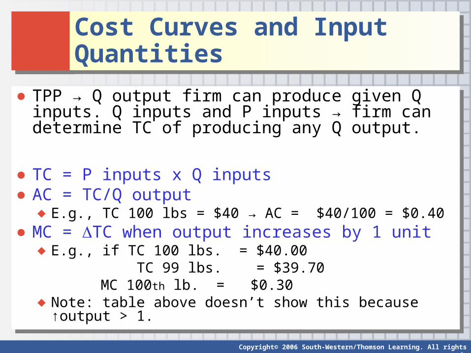
● TPP → Q output firm can produce given Q inputs. Q inputs and P inputs → firm can determine TC of producing any Q output.
● TC = P inputs x Q inputs● AC = TC/Q output
♦ E.g., TC 100 lbs = $40 → AC = $40/100 = $0.40● MC = TC when output increases by 1 unit
♦ E.g., if TC 100 lbs. = $40.00 TC 99 lbs. = $39.70
MC 100th lb. = $0.30♦ Note: table above doesn’t show this because ↑output > 1.
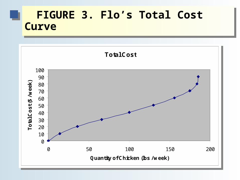
FIGURE 3. Flo’s Total Cost CurveFIGURE 3. Flo’s Total Cost Curve
Total Cost
0102030405060708090
100
0 50 100 150 200
Quantity of Chicken (lbs / week)
To
tal C
os
t ($
/ w
ee
k)
Total Cost
0102030405060708090
100
0 50 100 150 200
Quantity of Chicken (lbs / week)
To
tal C
os
t ($
/ w
ee
k)
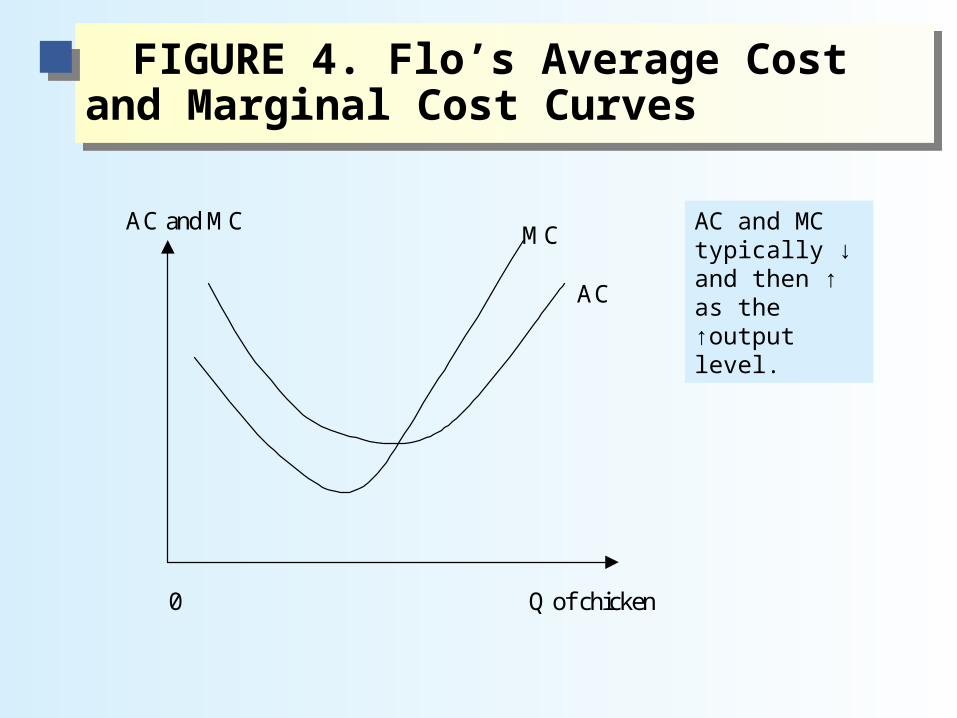
FIGURE 4. Flo’s Average Cost and Marginal Cost Curves
FIGURE 4. Flo’s Average Cost and Marginal Cost Curves
0
AC and MC
Q of chicken
MC
AC
AC and MC typically ↓ and then ↑ as the ↑output level.

Copyright© 2006 South-Western/Thomson Learning. All rights reserved.
● TC, AC, and MC can be divided into 2 parts –fixed costs and variable costs.
● Fixed cost is the cost of an input whose Q does not ↑ when ↑output. Input that the firm requires to produce any output. Any other cost is a variable cost.♦ E.g., takes at least 1 taxi to run a cab co. and its cost is the
same whether 1 or 60 people ride in it. But gas use rises as more people ride. Taxi is a fixed cost and gas is a variable cost.
What are the fixed and variable costs where you work?
Fixed and Variable CostsFixed and Variable Costs
Copyright© 2006 South-Western/Thomson Learning. All rights reserved.
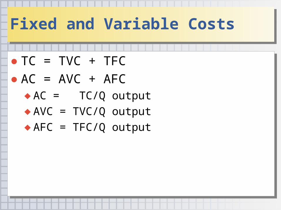
● TC = TVC + TFC
● AC = AVC + AFC♦ AC = TC/Q output♦ AVC = TVC/Q output♦ AFC = TFC/Q output
● TC = TVC + TFC
● AC = AVC + AFC♦ AC = TC/Q output♦ AVC = TVC/Q output♦ AFC = TFC/Q output
Fixed and Variable CostsFixed and Variable Costs

Table 4. Flo’s Total and Average Fixed Costs
Table 4. Flo’s Total and Average Fixed Costs
Output (20 lb pack)
TFC$ / week
AFC$ / week
0 5.0 ---
1 5.0 5.00
2 5.0 2.50
3 5.0 1.70
4 5.0 1.25
5 5.0 1.00
6 5.0 0.80
7 5.0 0.70
8 5.0 0.60
Flo pays rent of $5 per week for her chicken coop.

FIGURE 5. Graph of Flo’s Total Fixed CostFIGURE 5. Graph of Flo’s Total Fixed Cost
TFC
Q (20 lb. packages)
TFC$5
0 6 8 10
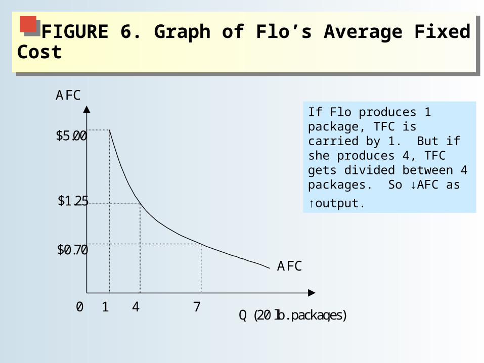
FIGURE 6. Graph of Flo’s Average Fixed CostFIGURE 6. Graph of Flo’s Average Fixed Cost
AFC
Q (20 lb. packages)
AFC
0 1
$5.00
4
$1.25
7
$0.70
If Flo produces 1 package, TFC is carried by 1. But if she produces 4, TFC gets divided between 4 packages. So
↓AFC as ↑output.
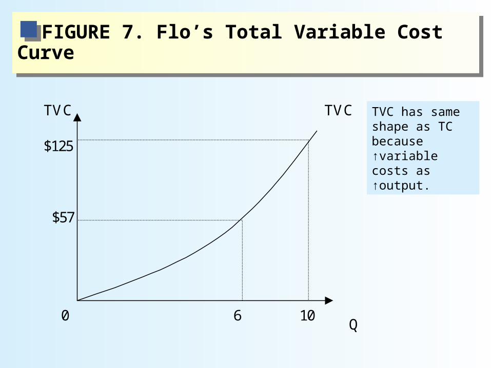
FIGURE 7. Flo’s Total Variable Cost CurveFIGURE 7. Flo’s Total Variable Cost Curve
TVC
Q
TVC
$125
0
$57
6 10
TVC has same shape as TC because ↑variable costs as ↑output.

Copyright© 2006 South-Western/Thomson Learning. All rights reserved.
● Marginal Cost = Marginal Variable Cost (MVC)
Why doesn't MC have a fixed component (i.e., MC = MVC + MFC)?
● Marginal Cost = Marginal Variable Cost (MVC)
Why doesn't MC have a fixed component (i.e., MC = MVC + MFC)?
Fixed and Variable Costs Fixed and Variable Costs
Copyright© 2006 South-Western/Thomson Publishing. All rights reserved.
Copyright© 2006 South-Western/Thomson Learning. All rights reserved.
● AC is generally U shaped –it initially declines and eventually rises with the level of output.
● AC declines for 2 reasons:1. Changing input proportions: at first, Flo feeds
chickens more corn while holding all other inputs constant. Output rises rapidly when ↑MPP corn, which tends to ↓AC.
2. ↓Average fixed costs as ↑output.
Shape of the Average Cost CurveShape of the Average Cost Curve
Copyright© 2006 South-Western/Thomson Publishing. All rights reserved.
Copyright© 2006 South-Western/Thomson Learning. All rights reserved.
● AC eventually rises for 2 reasons:1. Dim MPP: ↑output more slowly as ↓MPP corn,
which tends to ↑AC.2. Bureaucratic mess: as firms grow in size they lose
personal touch of management and become increasingly bureaucratic, which drives up costs.
● Point where ↑AC varies by industry. AC in auto industry begins ↑ after more units of output than farming. Huge K investment → AFC↓ dramatically.
Shape of the Average Cost CurveShape of the Average Cost Curve
Copyright© 2006 South-Western/Thomson Publishing. All rights reserved.
Copyright© 2006 South-Western/Thomson Learning. All rights reserved.
Short-run versus Long-run CostsShort-run versus Long-run Costs
● Cost of changing a firm's output level depends on period of time under consideration. Many input choices are precommitted by past decisions.
● Sunk cost = a cost to which a firm is precommitted for some limited period of time. ♦ E.g., a 2-year-old machine with a 9-year economic life is a
variable cost after 7 years because the machine would have to be replaced anyway.
Copyright© 2006 South-Western/Thomson Learning. All rights reserved.
Short-run versus Long-run CostsShort-run versus Long-run Costs
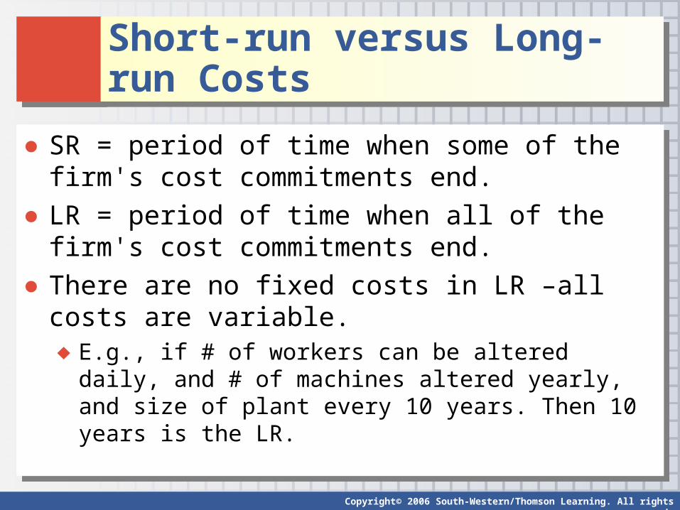
● SR = period of time when some of the firm's cost commitments end.
● LR = period of time when all of the firm's cost commitments end.
● There are no fixed costs in LR –all costs are variable.♦ E.g., if # of workers can be altered daily, and # of machines
altered yearly, and size of plant every 10 years. Then 10 years is the LR.
Copyright© 2006 South-Western/Thomson Learning. All rights reserved.
Short-run versus Long-run CostsShort-run versus Long-run Costs
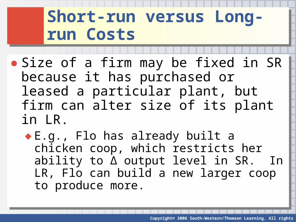
● Size of a firm may be fixed in SR because it has purchased or leased a particular plant, but firm can alter size of its plant in LR.♦ E.g., Flo has already built a chicken coop, which
restricts her ability to ∆ output level in SR. In LR, Flo can build a new larger coop to produce more.
● Size of a firm may be fixed in SR because it has purchased or leased a particular plant, but firm can alter size of its plant in LR.♦ E.g., Flo has already built a chicken coop, which
restricts her ability to ∆ output level in SR. In LR, Flo can build a new larger coop to produce more.
Copyright© 2006 South-Western/Thomson Learning. All rights reserved.
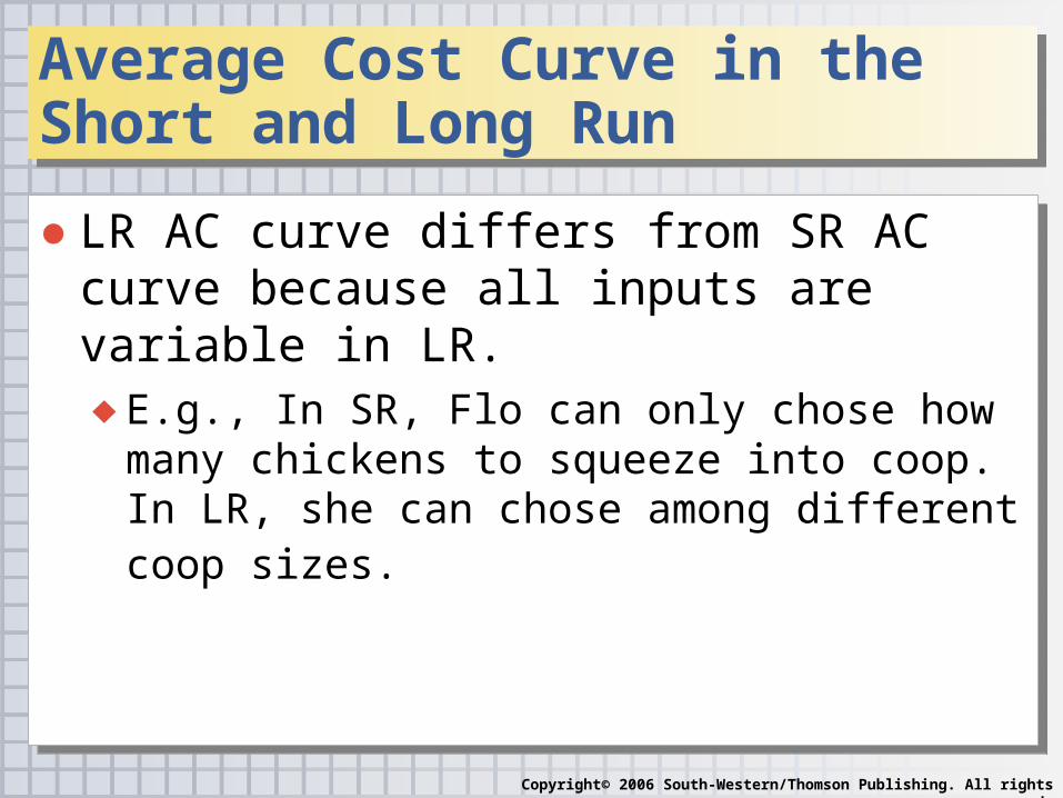
● LR AC curve differs from SR AC curve because all inputs are variable in LR.♦ E.g., In SR, Flo can only chose how many chickens to
squeeze into coop. In LR, she can chose among different coop sizes.
● LR AC curve differs from SR AC curve because all inputs are variable in LR.♦ E.g., In SR, Flo can only chose how many chickens to
squeeze into coop. In LR, she can chose among different coop sizes.
Average Cost Curve in the Short and Long RunAverage Cost Curve in the Short and Long Run
Copyright© 2006 South-Western/Thomson Publishing. All rights reserved.
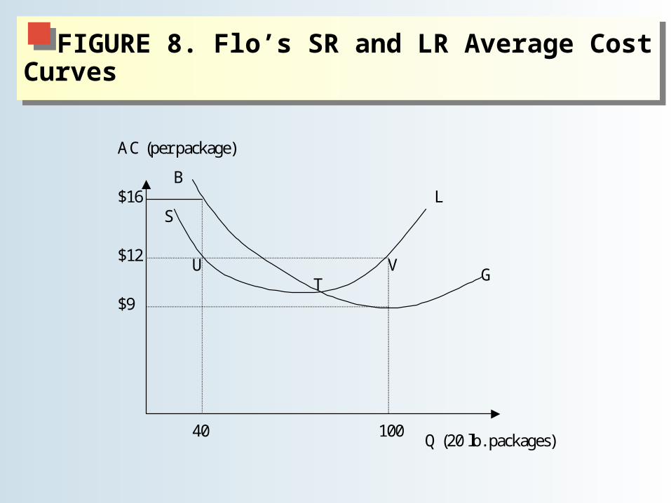
FIGURE 8. Flo’s SR and LR Average Cost Curves
FIGURE 8. Flo’s SR and LR Average Cost Curves
S$16
AC (per package)
Q (20 lb. packages)40 100
G
BL
VUT
$12
$9
Copyright© 2006 South-Western/Thomson Learning. All rights reserved.
Average Cost Curve in the Short and Long RunAverage Cost Curve in the Short and Long Run
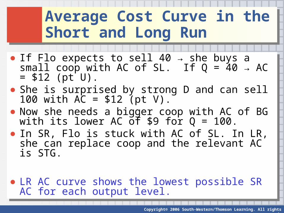
● If Flo expects to sell 40 → she buys a small coop with AC of SL. If Q = 40 → AC = $12 (pt U).
● She is surprised by strong D and can sell 100 with AC = $12 (pt V).
● Now she needs a bigger coop with AC of BG with its lower AC of $9 for Q = 100.
● In SR, Flo is stuck with AC of SL. In LR, she can replace coop and the relevant AC is STG.
● LR AC curve shows the lowest possible SR AC for each output level.
Copyright© 2006 South-Western/Thomson Learning. All rights reserved.
Economies of ScaleEconomies of Scale
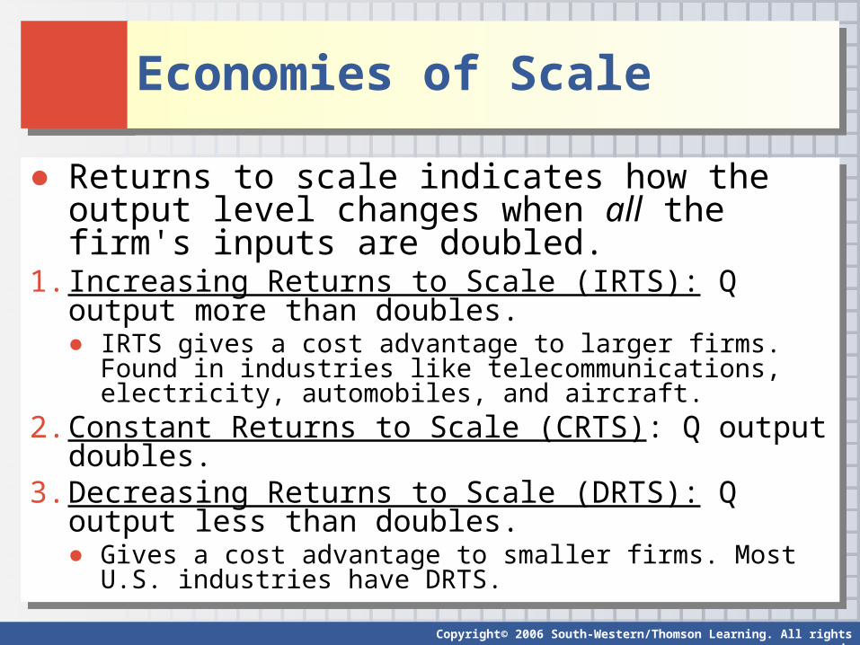
● Returns to scale indicates how the output level changes when all the firm's inputs are doubled.
1. Increasing Returns to Scale (IRTS): Q output more than doubles.● IRTS gives a cost advantage to larger firms. Found in
industries like telecommunications, electricity, automobiles, and aircraft.
2. Constant Returns to Scale (CRTS): Q output doubles.3. Decreasing Returns to Scale (DRTS): Q output less than
doubles. ● Gives a cost advantage to smaller firms. Most U.S. industries
have DRTS.
Copyright© 2006 South-Western/Thomson Learning. All rights reserved.
Economies of ScaleEconomies of Scale
● Returns to scale impacts the shape of the AC curve.
● AC = TC/Q output = (P input x Q input)/Q output♦ E.g., if Q inputs doubles and Q output doubles, then
AC is constant.
● Returns to scale impacts the shape of the AC curve.
● AC = TC/Q output = (P input x Q input)/Q output♦ E.g., if Q inputs doubles and Q output doubles, then
AC is constant.
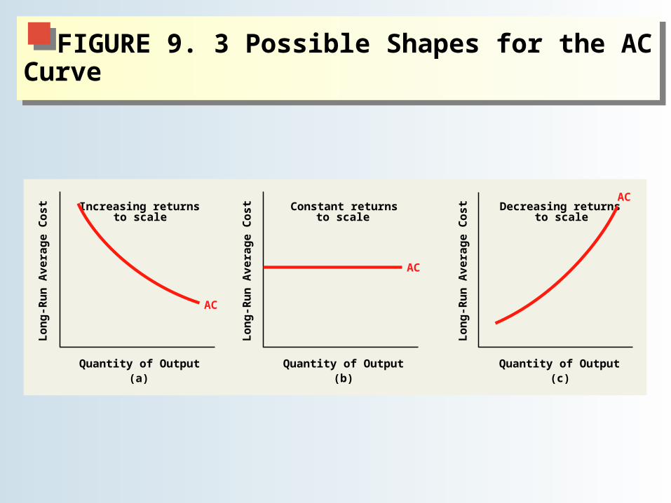
FIGURE 9. 3 Possible Shapes for the AC CurveFIGURE 9. 3 Possible Shapes for the AC Curve
Lo
ng
-Ru
n A
ve
rag
e C
os
t
(c) Quantity of Output
Decreasing returns to scale
Lo
ng
-Ru
n A
ve
rag
e C
os
t
(b) Quantity of Output
Constant returns to scale
Lo
ng
-Ru
n A
ve
rag
e C
os
t
(a) Quantity of Output
Increasing returns to scale
AC
AC
AC

Copyright© 2006 South-Western/Thomson Learning. All rights reserved.
Economies of ScaleEconomies of Scale
● Law of dim. marginal returns and IRTS may seem contradictory, but they are unrelated.
● Dim. marginal returns refers to increasing a single input. Returns to scale refers to a doubling of all inputs.
● A firm with dim. returns to a single input could have IRTS, CRTS, or DRTS.
● Law of dim. marginal returns and IRTS may seem contradictory, but they are unrelated.
● Dim. marginal returns refers to increasing a single input. Returns to scale refers to a doubling of all inputs.
● A firm with dim. returns to a single input could have IRTS, CRTS, or DRTS.