49th aiaa aerospace sciences meeting including … 2011-0203...aiaa-2010-0351 49th aiaa aerospace...

AIAA-2010-035149th AIAA Aerospace Sciences Meeting including the New Horizons Forum and Aerospace Exposition.

Numerical Study of Detonation–Turbulence Interaction

L. Massa, M. Chauhan and F.K. Lu,

Mechanical and Aerospace Engineering Department,

University of Texas at Arlington.

A numerical study is performed to investigate the effect of preshock turbulence on the

detonation wave properties. The analysis is based on the integration of the chemically

reactive Navier–Stokes equations using a Runge–Kutta scheme and a fifth-order WENO

spatial discretization. The results show a marked influence of preshock perturbations on

the postshock statistics. The alteration to the limit cycle structure supported by unstable

waves close to their critical points is highlighted. The effect of reactivity and fluid accel-

eration in the postshock region are examined by comparison with the non-reactive analog.

The possibility that significant forcing can lead to hot spot formation is investigated by con-

sidering temperature probability distribution functions in the reaction zone. The separate

effect of vortical and entropic fluctuations is considered.

I. Introduction

Many combustion processes are affected by the interaction between turbulence and heat release. Inparticular, detonation structures interact with a turbulized preshock field both during the initiation1 andthe propagation phases.2 Possible sources of turbulence ahead of a detonation wave are: turbulent boundarylayers resulting from gas dilatation in closed tubes (see Law3 p. 686), ridges in obstacle laden pipes,4

shock-flame interactions,5 and previous (detonation) waves in continuous spin detonation engines.6

The detonation–turbulence interaction problem in the present context is concerned with the unsteadycoupling between convected vortical/entropic structures and a detonation wave. Acoustic preshock fluctua-tions, although important to detonation initiation in obstacle-laden pipes (Law3 p. 686), are not consideredin the present study. The dynamics of the interaction reveals the role of preshock fluctuations on thepostshock field.

The non-reactive gas analog, shock–turbulence interaction, has been the subject of several theoretical,7, 8

numerical9–12 and experimental13, 14 investigations. A large portion of past numerical works was concernedwith comparing inviscid linear interaction analysis (LIA) with non-linear Navier-Stokes computations. Leeet al.9 analyzed the non-reactive coupling and found that non-linear computations agree well with Ribner’s7

LIA. While the linear analysis provides useful estimates of the amplification of vorticity fluctuations across theshock, it misses the strong nonlinear dynamics of the energized and highly anisotropic vorticity downstreamof the front.

Numerical simulation results presented by Rawat and Zhong12 indicated that transverse vorticity fluc-tuations are significantly enhanced across the shock and amplifications increased with the increasing Machnumber. Taylor microscales were seen to be reduced just behind the shock after which streamwise microscalesrapidly evolve. For turbulent Mach numbers approximately equal to 0.1 the non-linear amplification factorfor transverse microscales agrees well with the LIA results.

The detonation–turbulence interaction process differs from the non-reactive shock–turbulence analog be-cause of three reasons: exothermicity, the presence of a length scale associated with the detonation structure,and the presence of natural (intrinsic) fluctuations of the unstable detonation front. Jackson et al.17 con-ducted a linear interaction analysis of the reactive problem assuming that the reaction zone thickness is muchsmaller than the turbulence length scale. They, therefore, neglected both the effect of detonation structureand of intrinsic scales. They concluded that exothermicity affects the interaction of convected isotropic weak

Copyright c© 2010 by the authors.. Published by the American Institute of Aeronautics and Astronautics, Inc. withpermission.

1 of 27

American Institute of Aeronautics and Astronautics Paper AIAA-2010-0351

49th AIAA Aerospace Sciences Meeting including the New Horizons Forum and Aerospace Exposition4 - 7 January 2011, Orlando, Florida

AIAA 2011-203

Copyright © 2011 by the author(s). Published by the American Institute of Aeronautics and Astronautics, Inc., with permission.

turbulence by amplifying the rms fluctuations downstream of the detonation. The effect of exothermicity islinked to the Mach number, specifically the greatest changes occur around the Chapman-Jouguet condition.

Massa and Lu18 extended Jackson’s analysis by including the effect of the length scale associated withthe heat release. They found a strong dependency of the transfer functions on the perturbation wave numberthrough the ratio between fluctuation wavelength and half reaction distance. This phenomenon is absentin shock–turbulence LIA. They showed the existence of resonant wavelengths at which preshock Fouriercomponents are maximally amplified, leading to local maxima in postshock energy spectra. They relatedthe resonant wavelengths with neutral stability conditions (critical points) for the normal mode eigenvalueproblem of Short and Stewart.19 For linearly unstable waves, resonant wave numbers are loci of infiniteamplification of postshock power-spectra. Therefore, linear analysis provides useful insights but fails tocorrectly represent the system dynamics near natural frequencies.

Near the critical point of instability a viscous unstable detonation undergoes Hopf bifurcations to a limitcycle solution. A theoretical proof of the existence of closed orbits for one-dimensional, strong, viscous, det-onations was recently devised by Texier and Zumbrun.20 In a multi-dimensional study, Dou et al.21 studiedthe influence of transverse waves on the heat release zone and on the pattern of quasi-steady detonationfronts. They determined that the triple points generated by the motion of transverse waves causes the deto-nation front to become locally over-driven and form “hot spots” where chemical reaction is enhanced by thecoupling of high pressure and high velocity flow. Austin22 linked the disruption of the regular, periodic, limitcycle structure, and the formation of hot spots in unstable detonations to the mixture effective activationenergy.

The present work studies the effect of preshock turbulence on the limit cycle fluctuations. Noise can have arange of effects on an unstable dynamical system, which include stabilization,23 transition,24 and resonance.25

The dynamics of small fluid-mechanics scales is essential to resolving the thermo-fluid interaction in theinduction region of a detonation. Both vortical and entropic fluctuations in the preshock field are consideredin what is referred to as a forced detonation.

The paper is essentially divided in two parts. The first details the linear interaction analysis (LIA) thesecond the non-linear forced response.

II. Linearized Perturbation Equations

The linear perturbation equations in the postshock region are obtained from the compressible Eulerreactive equations by ignoring second-order contributions and setting the time derivative operator,

∂

∂t= V

∂

∂y,

where V = u0 tan θ0 is the velocity of the steady inertial reference frame defined by Ribner.16 The pertur-bation equations are written with respect to a reference system lying on a plane perpendicular to the shockplane and containing the wave number vector ~k. In this system, x (without subscript) is the direction normalto the shock and y is the direction parallel to it. The component of the wave number vector on the y axisis ky = k |cos (θ0)|. The postshock turbulence components are thus determined in the cylindrical referencesystem (x, y, φ) with associated wave number components (k1, ky, 0). The transverse wave number ky

is unchanged across the shock, while the longitudinal is different from the preshock analog. In the steadyreference frame attached to the shock wave, the postshock mean solution features the two flow angles,

θ1 ≡ tan−1

[

tan θ0M2

1 (γ − 1) + 2

(γ + 1)M21

]

,

immediately after the shock, and

θ∞ ≡ tan−1

tan θ0

(

2 + (γ − 1)M21

)

1 + γM21 −

√

(1 − M21 )

2 − 2Qc20/γ (γ2 − 1)M2

1

,

2 of 27


in the farfield. Here, M1 is the Mach number immediately after the shock, which is a function of the preshockMach number M0 only, or, by means of a more complex expression, of the detonation structure parameters,

M21 =

f(γ − 1)(

γQ − Q/γ +√

(γ2 − 1)Q (2γ + (γ2 − 1)Q)/γ + 1)

+ 2

−γ + 2f(

γ(

γQ +√

(γ2 − 1)Q (2γ + (γ2 − 1)Q)/γ + 1)

− Q)

+ 1. (1)

The solution array is composed by the complex transfer functions,

z ≡ [Xρ, Xu, Xv, Xp, Xλ]T,

plus the ratio between the shock front angle and the longitudinal velocity component of the preshock shearwave σ. Denoting by Z the mean-flow solutions,

Z ≡ [ρ, u, v, p, λ]T,

and changing to a shock-fitting coordinate system,

x → x − Ψ (y, t) ,∂Ψ

∂y= tanσ,

we obtain the following vector equation,

A∂z

∂x+ (B + V D)

∂z

∂y+ Cz − (B + V D)

∂Z

∂xσ = 0. (2)

The 5 × 5 matrices denoted with bold typeface are

A ≡

u ρ 0 0 0

0 u 0 1γρ 0

0 0 u 0 0

0 T − u2 0 0 0

0 0 0 0 u

, B ≡

0 0 ρ 0 0

0 0 0 0 0

0 0 0 1γρ 0

0 0 T 0 0

0 0 0 0 0

, (3)

C ≡

∂u∂x

∂ρ∂x 0 0 0

− ∂p∂x/

(

ρ2γ)

u 0 0 0

0 0 0 0 0

ζrρ − Tρ

∂u∂x −2u∂u

∂x 0 ζrp + ∂u∂x/ρ ζrλ

−rρ∂λ∂x 0 −rp −rλ

, D ≡

1 0 0 0 0

0 1 0 0 0

0 0 1 0 0

0 −u 0 1ργ 0

0 0 0 0 1

. (4)

where ζ = −Qc20 (γ − 1) /γ and the derivatives of the rate term with respect to density, pressure, and progress

variable are:

rρ = −rEc20

p, rp = rE

ρc20

p2, rλ = −K exp

(

−Eρc2

0

p

)

. (5)

The solution of equation (2) is converted from shock-fitted back to Cartesian coordinates using

z → z − ZxΨ (y, t) .

The evaluation of the auto-correlation in the wave number space, equation (12), and the linearity of theproblem allow us to analyze each Fourier component individually, so that the substitution ∂z/∂y → ikyzyields a system of ordinary differential equations in x. The linear system requires six boundary conditions,five are imposed at the shock front, and one at the farfield, x → ∞. The shock boundary conditions areobtained by linearization of the Rankine-Hugoniot shock relations. They are written in vector form as

z (γ + 1) = Sa

cos θ1/ cos θ0√

4 cos2 θ1 (1 − M21 ) (γM2

1 + 1) + M41 (γ + 1)2

+ Sb

tan θ1

M21 (γ − 1) + 2

σ, (6)

3 of 27


where the 5 × 1 arrays on the right-hand side are defined below,

Sa ≡

4/M1 (1 − γ) + 8γM1(

M21

(

γ2 − 6γ + 1)

+ 4 (γ − 1))

sec θ1

4(

1 + γ(

2M21 − 1

))

tan θ1

4γM1

(

M21 (γ − 1) + 2

)

0

, (7a)

Sb ≡

−4(

1 + γ(

2M21 − 1

))

2M1 sec θ1

(

M21 (3γ − 1) + 3 − γ

)

4/M1

(

(1 − 2γ)M41 + (γ − 3)M2

1 +(

γM41 + 1

)

cos(2θ1) + 1)

csc(2θ1)

−4γM21

(

M21 (γ − 1) + 2

)

0

. (7b)

The farfield condition is obtained by imposing no left-running characteristics, practically nullifying theupstream traveling acoustic wave. This condition is similar to that proposed by Short and Stewart,19 buthere we include the dependence of the solution on λ. This modified approach reduces the extension of thecomputational domain in x, and facilitates the task of integrating equation (2) for large wave numbers ky.In order to do so, we replace in equation (2)

∂z

∂x→ αz,

∂z

∂y→ ikyz,

and solve for the α (generalized) eigenvalues and the associated right eigenvectors matrix, R. The finalcondition is obtained by substituting in the eigenvectors matrix the column corresponding to the upstreamacoustic with the solution vector −z and imposing that the determinant of such matrix is equal to zero. Ina vector form, we write Sc

T z = 0, where

Sc ≡

0

Sd2Se5

Sd3Se5

Sd4Se5

SdTSe

, Sd ≡

0

V

−u

i/(ργ)√

1 − M2w

0

,

Se ≡

0

rλu (−irλ − kyV ) ζ

kyrλu2ζ

iζr2λu2ργ

iT((

u2 + V 2)

k2y + 2irλV ky + r2

λ

(

M2∞

− 1))

,

(8)

and Mw ≡√

(u2∞

+ V 2) /T∞ and M∞ ≡√

u2∞

/T∞ = Mw cos θ∞ are the farfield (burnt gas side) Machnumbers in the steady and shock reference frames, respectively. Note: all the flow variables in equation (8)are evaluated in the farfield and the superscript ∞ is dropped for brevity of notation.

II.A. Preshock Turbulence

The preshock turbulence field is assumed to be isotropic, frozen and divergence-free so that the velocity fieldis obtained as the superimposition of planar vorticity (shear) waves as described in more detail by Ribner.7

The von Karman spectral model is used to determine the ratio of the longitudinal velocity spectral densityto its mean square value. The von Karman spectral energy E (k) decays ∝ k−5/3 for k → ∞, it ignoresthe dissipation subrange, and is, therefore, an accurate model for high Reynolds number turbulence.26 Forthis reason, the von Karman model is commonly used in shock–turbulence inviscid LIA.7, 9 In sphericalcoordinates (k, θ0, φ),

[uu]0

u20

=Bk2 cos2 θ0

2π(

1 + k2)17/6

; (9)

4 of 27


where,

k = kaL∗, B =55

18πa, a =

55

27πB (1/3, 5/2) , (10)

and B denotes the Beta function.

II.B. Postshock Turbulence

The amplification of a wave pattern as it goes through the detonation is estimated in terms of auto-correlations. We seek to determine postshock turbulence auto-correlations by integrating the “transferred”wave amplitudes over the preshock wave number space. The evaluation of the transfer functions will beshown in detail in §II. The postshock turbulence is homogeneous on planes parallel to the unperturbedshock front (orthogonal to x1) and in time. A scalar field α (~x, t) is expanded over the (x2, x3, t) space inFourier-Stieltjes series in the general form

α (~x, t) =

∫

ei[k2,k3,kt]T [x2,x3,t] dZα (k2, k3, kt; x1), (11)

where k2 and k3 are the wave number vector projections onto the respective Cartesian axes, and kt = k1Ds,where Ds is the detonation Mach number based on the postshock speed of sound. Considerations aboutthe homogeneity of the scalar field (see, for example, Moyal27) lead to expressing the auto-correlation as anintegral over the wave number space,

α2 (x1) =

∫∫∫

[αα] (k2, k3, kt; x1) dk2 dk3 dkt; (12)

where [αα] is the spectral density over(

k2, k3, kt

)

. The transfer function Xα is defined such that

[αα] dk2 dk3 dkt = |Xα|2 [uu]0 dk1 dk2 dk3, (13)

so that integration is performed over the preshock wave number field. Integration over k2 and k3 defines theone-dimensional power spectrum,

Φα

(

k1

)

=

∫∫

|Xα|2[uu]0

u20

dk2 dk3. (14)

Substitution of equation (9) in equation (14) and conversion from Cartesian to spherical coordinates7 leadto

Φα =B

∣

∣

∣k1

∣

∣

∣

5/3

∫

|Xα|2cos3 θ0

sin5 θ0

(

k−21 + sin−2 θ0

)17/6dθ0. (15)

Note that the power spectra are integrated in k1 ∈ [−∞,∞], the longitudinal wave number in the preshockfield.

The transfer function depends on the wave number ~k. This is different from the two limiting cases ofJackson et al.28 and Ribner7 where it was a function of the angle θ0 only. The dependence of the transferfunction on k highlights the importance of the turbulence scaling effects, here represented by the variableL∗, which were ignored in previous discussions. It will be shown that the eigenvalues of the linear interactionhomogeneous problem play a significant role on the dependency of the transfer functions on the wave number.

III. LIA Results

III.A. Activation Energy Effect on Variances and Microscales

For L∗ → ∞ the activation energy does not affect the transfer functions (i.e. Jackson et al.’s theory28). Inthis section we seek to identify the effect of E on the turbulence amplification for finite wave thicknesses, andlink it to changes in characteristic solutions of the homogeneous problem described in ref.18 Referring to thestability analysis,19 we start with a stable detonation structure close to the instability boundary by setting

5 of 27


Q = 2, E = 10, γ = 1.2, f = 1.2, and L∗ = 1. The free-stream Mach number M0 = 1.9439 is independentof the activation energy, and will be used for comparison with the non-reactive interaction.

It was shown in ref.18that the activation energy plays a significant role on the energy spectra of finitethickness, weakly stable detonations by moving poles of the associated homogeneous problem with respectto the real axis. The emphasis of the present analysis is on the effect of the detonation structure on firstorder statistics, i.e. autocorrelations and length scales.

Longitudinal compression of fluid particles as they pass through the shock leads to a postshock turbulencewith axial symmetry, and decreases both the longitudinal velocity variance u2 and the longitudinal Taylor’smicroscale,9

λ1 ≡

√

√

√

√

u2

(

∂u∂x

)2.

Both quantities recover immediately after the shock as a result of the decay of the acoustic subcriticalcontributions to the velocity field. The non-linear analysis of Massa et al.29 determined that the u2 recoveryis significantly reduced in reactive conditions, while λ1 increases faster than in the non-reactive case.

The longitudinal Taylor’s microscale is infinite in the von Karman model because

limk1→∞

Φux,0 (k1) = limk1→∞

36k21Γ(

176

)

55√

π (k21 + 1)

5/6Γ(

13

)

(aL∗)26= 0, (16)

where Γ is the gamma function, and the factor (aL∗)2 is present in the denominator of equation (16) becauseL1/2 is the length scale. Nonetheless, the ratio between preshock and postshock Taylor’s microscale is finite,and by using the l’Hopital’s rule

λ1 =

√

u2

u20

limk1→∞

Φux,0 (k1)

Φux (k1), (17)

where Φux is determined from equation (15) with Xux = ∂Xu/∂x. The ratio under limit in equation (17)asymptotes to a constant value for k1 → ∞ and is evaluated at k1 = 30; differences between the values atk1 = 30 and k1 = 40 were found to be negligible.

The longitudinal velocity variance and Taylor’s microscale are plotted in the two panels of Fig. 1 fordifferent values of the activation energy, with the non-reactive solution corresponding to Ribner’s7 analysis.The LIA results are consistent with the non-linear analysis. Combustion increases the longitudinal varianceimmediately after the shock, while the larger postshock Mach number supports a weaker acoustic decay(in agreement with the results of Jackson et al.’s28). The longitudinal Taylor’s microscale is enhanced bycombustion, which selectively energize incoming wavelengths. An increase in activation energy augments theTaylor’s microscale effect.

III.B. L∗ Effect on a Detonation Close to the Stability Limit

An analysis of the longitudinal velocity variance and microscale for the L∗ 6= 1 cases is presented in Fig. 2.Close to the shock, the variance of the fluctuation is enhanced by an increase in L∗, while, far from thefront, its value is weakly affected. A similar observation holds for the microscale, for which a distinct peakis noted near the half reaction distance (x = 1) for large L∗. The weak dependence of the farfield velocitystatistics on L∗ is not surprising considering the spectra previously shown.18 Given that the temperaturespectra show a more substantial L∗ effect, the thermal fluctuation variance is analyzed in the next set ofplots.

Experimental observations correlate the presence of hot-spots to non-ideal preshock conditions.2 Thetemperature response to incompressible preshock turbulence is here analyzed based on the scaled varianceT 2/u2

0. Results are shown in Fig. 3 for different values of E and L∗. For the reactive cases, a global maximum

of T 2 is present within the reaction zone. This peak is pronounced and increases in magnitude with bothE and L∗, signaling the propensity for hot spot formation for higher activation energies and longitudinalscale of turbulence. The relationship between temperature amplification and E is consistent with Austin’s22

experimental observations on hot spot formation. Note that Austin did not consider a turbulent inflow, andthe postshock fluctuations were result of intrinsic instability; yet the experiments link spikes in temperaturedisturbances within the reaction zone to the activation energy.

6 of 27


0 2 4 6 8 10

0.8

1

1.2

1.4

1.6

1.8

x

u2

(a) Variance

0 2 4 6 8 10

0.1

0.2

0.3

0.4

0.5

0.6

x

λ1

Non−reactiveE=10E=5

(b) Microscale

Figure 1. Longitudinal velocity variance and Taylor’s microscale for Q = 2, E = 5, 10, γ = 1.2, f = 1.2, and L∗ = 1(M0 = 1.9439).

0 2 4 6 8 10

0.8

1

1.2

1.4

1.6

1.8

2

2.2

2.4

2.6

2.8

x

u2

(a) Variance

0 2 4 6 8 10

0.1

0.2

0.3

0.4

0.5

0.6

x

λ1

Non−reactive

L*=1

L*=5

L*=10

(b) Microscale

Figure 2. Longitudinal velocity variance and Taylor’s microscale for Q = 2, E = 10, γ = 1.2, f = 1.2, and L∗ = 1, 5, 10(M0 = 1.9439).

7 of 27


0 2 4 6 8 10

0.02

0.04

0.06

0.08

0.1

0.12

0.14

x

T2/u

2 0

Non−reactive

E=10, L*=1

E=5, L*=1

(a) Variance

0 2 4 6 8 10

0.2

0.4

0.6

0.8

1

1.2

x

T2/u

2 0

Non−reactive

E=10, L*=5

E=10, L*=10

(b) Microscale

Figure 3. Scaled temperature variance for Q = 2, E = 5, 10, γ = 1.2, f = 1.2, and L∗ = 1, 5, 10 (M0 = 1.9439).

IV. Non-Linear Analysis, Governing Equations

IV.A. Scales

The scales for the detonation–turbulence interaction problem are the root mean square of the longitudinalvelocity at the inflow urms,0, the inflow Taylor microscale λ0 based on the dissipation function, the preshockunperturbed density ρ0, and the specific gas constant R. This choice of scales is maintained for zero in-flow turbulence, the condition referred to as non-forced or natural detonation, by using the scales for thecorresponding forced case.

When performing linear analysis of detonation instability, the growth rate eigenvalue and associatedeigenfunctions are reported with a slightly different choice of scales. In such a case, the half detonationdistance L1/2 and the preshock pressure p0 are used in place of λ0 and urms,0. To avoid confusion, thescaling will be explicitly mentioned in the linear growth analysis.

IV.B. Navier–Stokes Equations

The governing equations are the non-dimensional conservative form of the continuity, momentum and energyequations in Cartesian coordinates. The working fluid is assumed to be a perfect gas.

∂ρ

∂t+

∂

∂xj(ρuj) = 0 (18a)

∂

∂t(ρui) +

∂

∂xj(ρuiuj + pδij − σij) = 0, i = 1, 2, 3 (18b)

∂Et

∂t+

∂

∂xj(Etuj + ujp + qj − uiσij) = 0 (18c)

∂ρλ

∂t+

∂(ρλuj + ρJj)

∂xj= (ρ − ρλ)r(T ), (18d)

where the viscous stress tensor, heat flux vector, and the mass diffusion velocity are

σ =µ

Re

(

∇~u + ∇~uT − 2

3I3,3∇ · ~u

)

, (19a)

~q = − γ

γ − 1

µ

RePr∇T, (19b)

8 of 27


ρ ~J = − µ

RePrLe∇λ (19c)

µ =

(

T

T0

)0.7

, (19d)

where I3,3 is the 3 × 3 identity matrix. The variable λ is the reaction progress, where λ = 0 describes theunburnt state and λ = 1 the completely burnt state. The total energy of the fluid is given by

Et = ρ

(

P

γ − 1+

u2i

2− Qλ

)

(20)

where Q is the non-dimensional heat release so that the term Qρλ denotes the non-dimensional chemicalenergy released as heat during the burning process. The reaction rate r(T ) is described by a single stepmechanism, where the Arrhenius law depends on temperature T through the relation

r(T ) = K0 exp

(

− E

T

)

(21)

where K0 is the pre-exponential factor that sets the temporal scale of the reaction, E is the non-dimensionalactivation energy.

V. Numerical Set-up

A sketch of the computational set-up for the study of turbulence detonation interaction is shown in Fig. 4.The domain is three-dimensional with a square transverse section (x− z) and periodic boundary conditionsat the x− y and x− z planes. Non-reflective boundary conditions are implemented at the subsonic out-flowboundary. The conditions at the supersonic inflow are detailed in §VI.A.

x

y

Shock Non−Reflective Boundary

x = 0

Figure 4. Sketch of the computational set-up.

VI. Test Cases

Consider a one–dimensional detonation structure with unit overdrive f = 1 and constant isentropic indexγ, there is a one-to-one relationship between inflow Mach number in shock reference frame M and heatrelease parameter,

Q ≡ Q

p0/ρ0=

Q

γM2t

=γ(

M2 − 1)

2

2 (γ2 − 1)M2, (22)

with Mt the turbulent Mach number. Note that Q is purely a detonation parameter and is independent ofthe inflow turbulence, while Q is an interaction parameter and depends on the inflow turbulence throughMt. Therefore, a one-dimensional detonation structure with unit overdrive can be identified by assigningM , E ≡ E/ (p0/ρ0) and γ.

In all cases considered, the isentropic index is kept fixed and equal to γ = 1.2. Two free-stream Machnumber conditions are considered in the present research. The low heat release case features M = 4.0 and,thus, Q = 19.18. The high heat release case has M = 5.5, which gives Q = 38.57.

9 of 27


The activation energy E can be physically related to responsive changes in induction time with thepostshock temperature in von Neumann conditions, (∂ln τi/∂lnTps)f=1, where τi is the induction time and

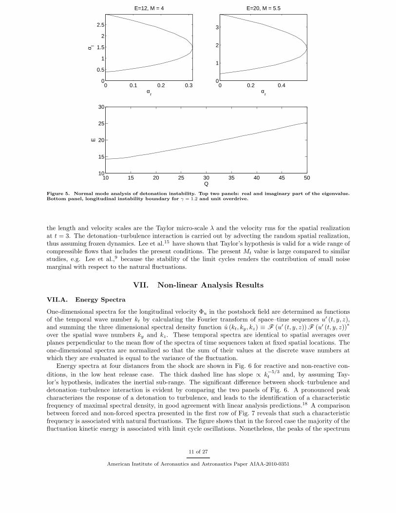
Tps is the postshock temperature.30 The choice of activation energy in the present study has been primarilydictated by selecting detonation structures that are longitudinally stable, i.e. , stable to one-dimensionalperturbations. Longitudinal instability gives rise to axial motion of the mean shock front and gallopingwaves,20 which complicates the evaluation of the ensemble average as a time-space mean at a fixed normal-to-the shock distance. The longitudinal instability boundary divides the E −Q quarter plane in two convexregions. Such a boundary for γ = 1.2 and unit overdrive is shown in the bottom panel Fig. 5. Based onthis figure, the choices E = 12 and E = 20 are made for low (Q = 19.18) and high (Q = 38.57) heat releasecases, respectively. The high heat release conditions are similar to those used by Dou et al.21 who simulateda detonation wave with Q = 50, E = 20, γ = 1.2 and f = 1.

Dissipation effects lead to the definition of the Reynolds number Reλ which will be set based on thedecay of homogeneous isotropic turbulence described in §VI.A, the Prandtl and Lewis numbers, which arefixed to Pr = 0.72 and Le = 1. Compressibility effects in the incoming turbulent flow are set by assigningthe turbulent Mach number Mt ≡ urms/

√

γp0/ρ0, which leads to the determination of the mean preshockpressure p0. The value of Mt is discussed in §VI.A. The final model parameter K0 is assigned by imposingthe half reaction distance L1/2 through the ratio L∗ = L1/2/λ0, where L∗ represents a ratio of detonationto turbulent scales and is set equal to one in all test cases.

Note that the Reynolds number based on acoustic velocity and half reaction distance, ReL1/2≡ √

p0ρ0L1/2/µ0 =

ReλL∗/(√

γMt

)

, is quite small in the simulations presented. In fact, for L∗ = 1, typical values of Mt ≈ 0.2and Reλ small enough to allow for a direct numerical simulation (DNS) of the problem, ReL1/2

≈ 200. Anincrease in L∗ leads to a proportional increase in ReL1/2

, but also to a similar increase in domain size andcomputational requirements. Therefore, for practical reasons, the DNS presented here refer to a very thindetonation wave with, in practice, a sub-millimeter reaction distance. The influence of a small Reynoldsnumber on the growth rate of normal mode disturbances is analyzed in.29

Three simulations at low heat release are discussed, a reactive, a non-reactive and a non-forced one.The non-reactive corresponds to shock–turbulence interaction conditions, with free-stream Mach numberM = 4.0. The non-forced conditions are obtained by zeroing out the incoming turbulence so that onlynatural instability fluctuations are present in the postshock field. Similarly, three simulations at high heatrelease are considered. In this case, two different kinds of inflow turbulence are analyzed together withthe non-forced detonation. The first forced inflow case has only vortical waves, obtained from the decay ofhomogeneous turbulence described in §VI.A. In the second case, the vortical waves are nullified in favor ofentropy waves obtained using the Morkovin31 scaling: an empirical relationship between temperature andlongitudinal velocity perturbation valid in constant pressure boundary layers. Density fluctuations in theconstant pressure inflow are related to the isotropic turbulence velocity perturbation by

ρ′/ρ = (γ − 1)M2 u′

u. (23)

Mahesh et al.32 used equation (23) to analyze the influence of entropy perturbation on the shock–turbulenceinteraction, and discovered a strong influence of preshock density fluctuations on postshock perturbationdynamics.

VI.A. Inflow Boundary Conditions and Temporal Decay

The inflow boundary conditions are implemented by imposing the fluid state on the supersonic inflow side.The procedure is similar to that described by Mahesh et al.32 The flow is decomposed into a mean andperturbation part. The perturbation is evaluated by temporal decay of homogeneous, isotropic, compressibleturbulence in a cube with periodic boundary conditions. The initial spectrum is Gaussian and symmetricwith kinetic energy density

E (k) =16√

2π exp

(

− 2k2

k2

0

)

k4

k50

, (24)

with k0 = 3.The spatial realization used to model the inflow boundary conditions corresponds to the t = 3 solution,

for which the inflow turbulent Mach number is Mt = 0.235. The time-decayed turbulence is rescaled so that

10 of 27


0 0.1 0.2 0.30

0.5

1

1.5

2

2.5

αr

α I

E=12, M = 4

0 0.2 0.40

1

2

3

αr

E=20, M = 5.5

10 15 20 25 30 35 40 45 5010

15

20

25

30

Q

E

Figure 5. Normal mode analysis of detonation instability. Top two panels: real and imaginary part of the eigenvalue.Bottom panel, longitudinal instability boundary for γ = 1.2 and unit overdrive.

the length and velocity scales are the Taylor micro-scale λ and the velocity rms for the spatial realizationat t = 3. The detonation–turbulence interaction is carried out by advecting the random spatial realization,thus assuming frozen dynamics. Lee et al.15 have shown that Taylor’s hypothesis is valid for a wide range ofcompressible flows that includes the present conditions. The present Mt value is large compared to similarstudies, e.g. Lee et al.,9 because the stability of the limit cycles renders the contribution of small noisemarginal with respect to the natural fluctuations.

VII. Non-linear Analysis Results

VII.A. Energy Spectra

One-dimensional spectra for the longitudinal velocity Φu in the postshock field are determined as functionsof the temporal wave number kt by calculating the Fourier transform of space–time sequences u′ (t, y, z),and summing the three dimensional spectral density function u (kt, ky, kz) ≡ F (u′ (t, y, z))F (u′ (t, y, z))

∗

over the spatial wave numbers ky and kz. These temporal spectra are identical to spatial averages overplanes perpendicular to the mean flow of the spectra of time sequences taken at fixed spatial locations. Theone-dimensional spectra are normalized so that the sum of their values at the discrete wave numbers atwhich they are evaluated is equal to the variance of the fluctuation.

Energy spectra at four distances from the shock are shown in Fig. 6 for reactive and non-reactive con-

ditions, in the low heat release case. The thick dashed line has slope ∝ k−5/3t and, by assuming Tay-

lor’s hypothesis, indicates the inertial sub-range. The significant difference between shock–turbulence anddetonation–turbulence interaction is evident by comparing the two panels of Fig. 6. A pronounced peakcharacterizes the response of a detonation to turbulence, and leads to the identification of a characteristicfrequency of maximal spectral density, in good agreement with linear analysis predictions.18 A comparisonbetween forced and non-forced spectra presented in the first row of Fig. 7 reveals that such a characteristicfrequency is associated with natural fluctuations. The figure shows that in the forced case the majority of thefluctuation kinetic energy is associated with limit cycle oscillations. Nonetheless, the peaks of the spectrum

11 of 27


are smoothed and decreased in magnitude by the addition of inflow turbulence.A similar result is obtained by comparing forced and non-forced high heat release cases. The results

are shown in the second and third rows of Fig. 7 for vortical and entropy waves respectively. The peakfrequency is approximately constant when changing the distance from the shock and matches the frequencyof the most amplified linear wavelength as inferred from the top panels of Fig. 5. Due to the different non-dimensionalization used in the growth rate eigenvalue computations, α values in Fig. 5 must be multiplied by(

Mt√

γ)

−1to compare with the turbulent computations. After conversion to the inflow fluctuation scales,

the most amplified linear frequencies are 5.6 and 6.98 for the low and high heat release cases, respectively.The peak in response spectra are at kt = 5.2 and 6.91, for the analogous non-linear cases.

The two bottom rows of Fig. 7 also reveal that the entropy fluctuations are more effective in disruptingthe periodic limit cycle solutions supported by the intrinsic detonation instability. The difference betweenforced and non-forced cases is much larger in the bottom row of Fig. 7 than in the middle one.

100

101

10−2

kt

Φu

reactive

100

101

kt

Φu

non−reactive

X−Xs = 4

X−Xs = 6

X−Xs = 8

X−Xs = 10

Figure 6. One–dimensional energy spectra against temporal wave number. Comparison of reactive and non-reactive

cases with vortical inflow at M = 4. The thick dashed line is ∝ k−5/3

t .

12 of 27


10−4

10−2

Φu

X−Xs = 4 X−X

s = 6 X−X

s = 8 X−X

s = 10

10−4

10−2

Φu

100

101

10−2

kt

Φu

100

101

kt

100

101

kt

100

101

kt

Figure 7. One–dimensional energy spectra against temporal wave number: comparison of forced and non-forced cases.Each column represents a distance from the shock as indicated in the column titles. Top row, low heat release, M = 4;solid line non-forced and dashed line vortical forcing. Mid row, high heat release, M = 5.5; solid line non-forced anddashed line vortical forcing. Bottom row, high heat release, M = 5.5; solid line non-forced and dashed line entropic

forcing. In all panels, the thick dashed lines are ∝ k−5/3

t .

VII.B. Analysis of Variances and Auto-correlations

The forced and non-forced spectra presented in §VII.A reveal marked differences in the responses of reactiveand nonreactive configurations to a turbulent inflow. Such differences are investigated in more detail byanalyzing variances of the fluctuation where, as before, ensemble averages are computed as space–timeaverages at constant distance from the shock. In general, the use of so-called Favre averages (see, forexample, Warsi33 p. 481), used for example by Lee,9 changes the results only marginally, therefore non-weighted averages are used in all results presented in this work.

The meanflow structure is significantly affected by intrinsic and forced fluctuations. Figure 8 showsthe mean temperature and velocity for the five reactive cases along with the corresponding unperturbedZel’dovich-Neumann-Doering (ZND) profiles. For all cases, the jump across the shock is lower than thatpredicted by the Rankine–Hugoniot conditions. This phenomenon is a consequence of both shock frontmotion and corrugation, and is consistent with the mean shock profiles reported by Lele and Larson34 atlarge Mt and in non-reactive conditions. The reaction length supported by turbulent inflow L1/2 is evaluated

based on the mean profile as the distance between the location at which λ = 1 × 10−3 and that at whichλ = 0.5. For the low heat release condition, the non-forced and vorticity forced cases have L1/2 equal to1.840 and 1.542 respectively. For the high heat release condition, the non-forced, vorticity forced and entropyforced cases have L1/2 equal to 1.963, 1.889 and 2.312 respectively. The intermittent corrugation of the frontexpands the half reaction distance above the one-dimensional value of L1/2 = 1. Vorticity forcing aheadof the wave tends to reduce the region of heat release, with a more pronounced effect in low heat releaseconditions, while entropy forcing leads to an increase in L1/2.

Longitudinal and transverse velocity variances are shown for the six cases in Fig. 9. The top-row panelsrefer to the low heat release case and the solid, dashed and dotted curves represent non-reactive, non-forcedand vortical inflow solutions respectively. The major difference between shock–turbulence and detonation–

13 of 27


turbulence interaction is the loss of the longitudinal fluctuation peak immediately after the shock. Such alocal maximum is due to the decay of sub-critical acoustic waves (those which are damped in the postshockfar-field) followed by viscous dissipation, and is typical of non-reactive conditions as the linear interactionanalysis of Rawat and Zhong12 shows. Moreover, for the reactive cases, the presence of inflow vorticalfluctuations increases transverse fluctuations of up to 50% above the non-forced values, at selected locations.

Note in top-left panel of Fig. 9 that the non-reactive longitudinal correlation immediately after the shockis larger than its preshock value. This behavior is in contrast with that reported in literature.9, 12 Furtheranalysis shows that this result is a consequence of the high turbulent Mach number, and is associated to thelarge shock corrugation. In Fig. 10, such longitudinal variances are compared to a non-reactive Mt = 0.1case. The comparison shows that the low Mt case behaves similarly to literature data.9, 12 Moreover, theMt = 0.235 variance presents a much higher peak immediately after the shock, and drops below the low Mt

case far from the front.The two bottom panels of Fig. 9 refer to the high heat release case with solid, dashed and dotted

lines indicating non–forced, vortical and entropy wave solutions, respectively. Vortical fluctuations producea weaker increase in transverse variances in the high heat release case than in the low heat analog. Itis also evident that the limit cycles are less sensitive to vorticity forcing than to entropy forcing. Theinflow entropy fluctuation is more effective than the vortical analog in reducing the longitudinal velocityfluctuations associated with the detonation instability. Contrary to vorticity forcing, the addition of entropyforcing reduces postshock transverse fluctuations.

To provide a graphical analysis of the effects of turbulence on detonations, numerical schlieren snapshotsare shown in Figs. 11–13 for the three high heat release cases. All panels refer to an x − y slice at halfthe box size, z = L/2. Each panel represents a different time as indicated in the titles. The time sequencecovers approximately the period of the most amplified linear mode Tα = 2π/6.98 ≈ 0.9, which was previouslyshown to match the wave number of the maximum of the velocity spectra. The non-forced case shows atime periodicity typical of limit cycle solutions. Both forced cases display a more complex time history. Aconsiderably more perturbed postshock field is noticed in the entropy forced case, where large pockets ofhigh density material detach from the shock front and are convected downstream. These regions correspondwith unburned material convected through the reaction region. Temperature fluctuations in the fire zoneare amplified by the perturbed inflow (a more detailed analysis is presented in §VII.C), but no evidence ofhot spots is found.

Auto-correlations in planes parallel to the unperturbed shock front are presented in terms of integrallength scales. The scales are evaluated by integrating the correlation coefficient built on space–time averagesagainst the separation distance. The autocorrelation coefficient is a scaled two–point correlation function,so that the integral length associated to a general variable f takes the form,

Λf =

∫ L2

0 f (x, y, z, t)′

f (x, y + h, z, t)′

dh

σf, (25)

where σ is the variance. Davidson35 explained that autocorrelation helps in differentiating between thesmall and large scale eddies in turbulence, and is preferable to one–dimensional, scalar functions, such asux. It is conventional to evaluate the Fourier transform of the velocity correlation tensor Qij with diagonalcomponents Qii representing autocorrelation functions for the velocity components ui. Huang et al.36 arguedthat the autocorrelation function is a good indicator of the inertial sub-range.

Temperature, longitudinal velocity, density and progress of reaction (ΛT , Λu, Λρ, and Λλ) scales areplotted against the distance from the shock in the four panels of Figs. 14–15. The two figures show thestrong effect of natural detonation fluctuations in increasing the integral scales across the shocks. Theaddition of inflow turbulence breaks natural scales and considerably reduces the integral scale. Entropyinflow perturbations are found to be more effective than vorticity analogs in breaking regular structures.

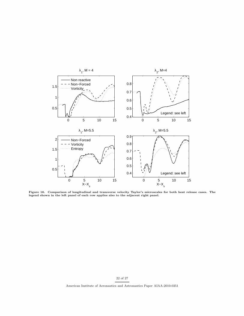
Longitudinal velocity and transverse velocity Taylor microscales, λ1 and λ2 are plotted in Fig. 16 for thetwo levels of heat release. The Taylor microscales are evaluated as

λ1 =

√

√

√

√

u′2

(

∂u′

∂x

)2, λ2 =

√

√

√

√

√

v′2

(

∂v′

∂y

)2. (26)

They are strongly affected by the reactivity of the mixture in the postshock field. The detonation–turbulenceinteraction supports significantly higher values of the microscale than the nonreactive analog. Nevertheless,

14 of 27


the distribution of the microscale in the postshock field is not significantly affected by an increase in heatrelease. The addition of a turbulent inflow has also a marginal effect on the microscale. This conclusionis in contrast with that drawn for the integral scale. The longitudinal microscale for the reactive cases issignificantly larger than the transverse one, showing the effect of combustion in energizing (accelerating)longitudinal structures at selective wave numbers. The selectivity of the reactive interaction is in agreementwith the results of linear analysis,18 and the presence of local maxima in the post shock spectra shown in§VII.A. Entropy fluctuations behaving according to Morkovin’s hypothesis are more effective in reducingthe microscale in the postshock field than the vortical analogs.

0 5 10 151

2

3

4

5T

M = 4

0 5 10 15

5

10

15

u

M=4

ZNDNon−ForcedVorticity

ZNDNon−ForcedVorticity

0 5 10 15

2

4

6

8

X−Xs

T

M=5.5

0 5 10 15

5

10

15

20

X−Xs

u

M=5.5

ZNDNon−ForcedVorticityEntropy

ZNDNon−ForcedVorticityEntropy

Figure 8. Temperature and longitudinal velocity means for the five reactive cases. ZND profiles refer to the classicalone-dimensional, steady analysis of detonation waves.

15 of 27


0 5 10 150

2

4

6

8

10M = 4, Longitudinal

0 5 10 150

1

2

3

4

5

M=4, Transversal

Non reactiveNon−ForcedVorticity


0 5 10 150

2

4

6

8

10

X−Xs

M=5.5, Longitudinal

0 5 10 150

2

4

6

8

10

X−Xs

M=5.5, Transversal

Non−ForcedVorticityEntropy


Figure 9. Longitudinal and transverse velocity variances for different inflow forcing and Mach numbers.

16 of 27


−2 0 2 4 6 8 10 12 14 160

1

2

3

4

5

6

X−Xs

σ u

Mt = 0.1

Mt = 0.235

Figure 10. Comparison of low and high Mt non-reactive cases variances at M = 4.

17 of 27


Figure 11. Numerical schlieren for the non-forced M = 5.5 case. Different panels refer to the same z = L/2 slice butdifferent times, as indicated on top of each panel. The time-interval 15.0− 15.9 corresponds with the period of the mostamplified normal mode Tα = 2π/6.98 ≈ 0.9.

VII.C. Probability Distribution Functions

A set of probability distribution functions (PDF) is evaluated in the post-shock region by determiningconditional probabilities for λ < 0.5 and p > pZND/2, where pZND is the maximum pressure for a steadydetonation wave. The conditional probability functions for longitudinal velocity and temperature are plottedfor all cases in Fig. 17. For both heat release cases, the response to vortical forcing leads to a largerrange of fluctuations. The changes in both u and T fluctuations are substantial in the near-shock region.Entropy fluctuations support stronger changes than vortical fluctuations. The temperature PDF for theentropy forcing case manifests a significant increase at large temperatures, which points to the possibility ofsupporting hot spot formation at higher activation energies.

Changes in fluctuations caused by the turbulent inflow decrease downstream of the shock plane, asdemonstrated by longitudinal velocity PDFs evaluated at different downstream locations (x = constant)shown in Figs. 18 and 19. The marked difference between reactive and non reactive longitudinal velocityPDF shown in Fig. 18 is due to gas acceleration caused by the reactivity. The temperature PDF (notshown) behaves similarly to the velocity counterpart: differences caused by the forcing quickly diminish asthe distance from the shock is increased, leading to a downstream PDF that is weakly dependent on theinflow perturbation.

VIII. Conclusions and Future Work

The present research examines the interaction of turbulence with a detonation wave from both the linearand non-linear standpoints. The focus is on changes with respect to the shock–turbulence analog as aconsequence of the reactivity. Nonlinear calculations are carried out to investigate modifications to thelimit-cycle natural fluctuations caused by strongly perturbed inflows. Linear interaction analysis is limitedto weakly stable (i.e. close to the stability boundary) conditions, and explains the role of system naturalfrequencies on first order statistics.

The main conclusions of the present work are summarized below. For a turbulent Mach number Mt =

18 of 27


Figure 12. Numerical schlieren for the vorticity perturbation M = 5.5 case. Different panels refer to the same z = L/2slice but different times, as indicated on top of each panel.

Figure 13. Numerical schlieren for the entropy perturbation M = 5.5 case. Different panels refer to the same z = L/2slice but different times, as indicated on top of each panel.

19 of 27


0 5 10 15

0.5

1

1.5

2

ΛT, M = 4

0 5 10 15

1

1.5

2

Λu, M = 4

0 5 10 150.5

1

1.5

2

X−Xs

Λρ, M = 4

0 5 10 15

0.5

1

1.5

2

X−Xs

Λλ, M = 4


Figure 14. Comparison of integral length scales for the low heat release case. The legend shown in the bottom-rightpanel applies to all. In the bottom right panel, the non-reactive curve is not drawn because the progress of reaction isnot defined.

20 of 27


0 5 10 15

0.5

1

1.5

2

2.5

ΛT, M = 5.5

0 5 10 15

0.5

1

1.5

2

Λu, M = 5.5

0 5 10 150.5

1

1.5

X−Xs

Λρ, M = 5.5


0 5 10 15

0.5

1

1.5

2

2.5

X−Xs

Λλ, M = 5.5

Figure 15. Comparison of integral length scales for the high heat release case. The legend shown in the bottom-leftpanel applies to all.

21 of 27


0 5 10 15

0.5

1

1.5

λ1, M = 4

0 5 10 150.4

0.5

0.6

0.7

0.8

λ2, M=4

Legend: see left


0 5 10 15

0.5

1

1.5

2

X−Xs

λ1, M=5.5

0 5 10 15

0.4

0.5

0.6

0.7

0.8

0.9

X−Xs

λ2, M=5.5

Legend: see left


Figure 16. Comparison of longitudinal and transverse velocity Taylor’s microscales for both heat release cases. Thelegend shown in the left panel of each row applies also to the adjacent right panel.

22 of 27


2 4 60

2

4

6M = 4, Temperature

−10 0 10 200

0.1

0.2

0.3M=4, Longitudinal

Legend: see leftNon reactiveNon−ForcedVorticity

0 5 100

0.1

0.2

0.3

T/T0

M=5.5, Temperature

−10 0 10 200

0.05

0.1

0.15

0.2

u/urms,0

M=5.5, Longitudinal

Legend: see leftNon−ForcedVorticityEntropy

Figure 17. Conditional PDF of temperature and longitudinal velocity for λ < 0.5 and p > pZND/2, i.e. , in the reactionzone.

23 of 27


−5 0 5 100

0.1

0.2

0.3

0.4

M=4, X−Xs = 4

0 5 100

0.1

0.2

0.3

0.4

M=4, X−Xs = 6

0 5 100

0.1

0.2

0.3

0.4

0.5

M=4, X−Xs = 8

u/urms,0

0 5 100

0.1

0.2

0.3

0.4

0.5

M=4, X−Xs = 10

u/urms,0


Figure 18. Low heat release longitudinal velocity PDF at constant x, for various distances from the shock. The legendshown in the top-left panel applies to all four panels.

24 of 27


0 5 10 150

0.1

0.2

0.3

M=5.5, X−Xs = 4

5 10 150

0.05

0.1

0.15

0.2

0.25

M=5.5, X−Xs = 6

5 10 150

0.05

0.1

0.15

0.2

M=5.5, X−Xs = 8

u/urms,0

6 8 10 12 14 160

0.1

0.2

0.3

M=5.5, X−Xs = 10

u/urms,0


Figure 19. High heat release longitudinal velocity PDF at constant x, for various distances from the shock. The legendshown in the top-left panel applies to all four panels.

25 of 27


0.235, postshock fluctuations in reactive conditions are dominated by wavelengths associated with the naturalfluctuations. The introduction of vortical and entropy perturbations reduces, but does not shift, peakintensities in the one-dimensional kinetic energy spectra. Transverse velocity variances are considerablyaugmented above the unforced value by both vortical and entropic fluctuations. The reactivity in the post-shock region eliminates the peak in longitudinal variance due to the contribution of sub-critical acoustics tovelocity components. Both linear and nonlinear analysis agree in this respect.

Integral length scales are markedly increased by natural (limit cycle) oscillations above the nonreactivevalues. Entropy fluctuations are more effective than vorticity analogs in reducing the integral scales. Taylormicroscales based on the velocity components are increased by reactivity, which considerably stretches smallstructures in the longitudinal direction. Different from the integral length scale case, the addition of pre-shock forcing weakly affects velocity microscales. Probability distribution functions for forced cases manifesta flattened profile when compared to detonations propagating in unperturbed fields.

Both forcing conditions lead to an increased probability of high temperature fluid in the reaction zone.Linear analysis shows the presence of a substantial peak of the temperature variance in the reaction regionfor high activation energies. It is, therefore, the structure of the reactive region that leads to thermalamplification, and possibly to the formation of hot spots. Entropy forcing leads to the formation of largepockets of unburned material, detached from the shock. These effects are also present in vortical forcingcases, but are of reduced magnitude.

Future work will focus on two aspects of detonation–turbulence interaction. First is the analysis of largeactivation energies, beyond the longitudinal stability limit. Based on present results, large activation energiesare likely to support hot spot formation for strong inflow forcing. Second, large N and Re numbers will beinvestigated using a large eddy simulation (LES) approach built upon the present DNS effort.

References

1G. Ciccarelli and S. Dorofeev. Flame acceleration and transition to detonation in ducts. Prog. Energy Combust.Sci. 34:499, (2008).

2B.E. Gelfand, S.M. Frolov and M.A. Nettleton. Gaseous detonations. A selective review. Prog. Energy Combust.Sci. 17:327-371, (1991).

3C.K. Law. Combustion Physics. Cambridge University Press (2006).4S.B. Dorofeev, M.S. Kuznetsov, V.I. Alekseev, A.A. Efimenko, and W. Breitung. Effect of scale on the onset of detonations.

Shock Waves 10:137, (2000).5A.M. Khokhlov, E.S. Oran, A.Y. Chtchelkanova and J.C. Wheeler. Interaction of a shock with a sinusoidally perturbed

flame. Combust. Flame 117:99, (1999).6F.A. Bykovskii, S.A. Zhdan, and E.F. Vedernikov. Continuous Spin Detonations. J. Propulsion Power 22:1204, (2006).7H.S. Ribner. Spectra of Noise and Amplified Turbulence Emanating from Shock–Turbulence Interaction. AIAA

J. 25(3):436–442, (1987).8S.L. Gavrilyuk and R. Saurel. Estimation of the turbulent energy production across a shock wave. J. Fluid Mech. 549:131,

(2006).9S. Lee, S.K. Lele, and P. Moin. Interaction of Isotropic Turbulence with Shock Waves: Effect of Shock Strength. J. Fluid

Mech. 340:225-247, (1997).10S. Jamme, J.B. Cazalbou, F. Torres, and P. Chassaing. Direct numerical simulation of the interaction between a shock

wave and various types of isotropic turbulence. Flow, Turbulence and Combustion 68:227-268, (2002).11F. Ducros, V. Ferrand, F. Nicoud, C. Weber, D. Darracq, C. Gacherieu, and T. Poinsot. Large eddy simulation of the

shock/turbulence interaction. J. Comp. Phys. 152:517-549, (1999).12P.S. Rawat and X. Zhong. Numerical Simulation of Shock–Turbulence Interactions using High-Order Shock-Fitting Al-

gorithms. AIAA 2010-114, Orlando, FL, (2010).13J.H. Agui, J. Briassulis and G. Andropoulos. J. Fluid Mech. 524:143, (2005).14S. Xanthos, M. Gong and G. Andropoulos. Velocity and vorticity in weakly compressible isotropic turbulence under

longitudinal expansive straining. J. Fluid Mech. 584:301, (2007).15S. Lee, S.K. Lele, and P. Moin. Simulation of spatially evolving turbulence and the applicability of Taylor’s hypothesis

in compressible flow. Phys. Fluids A 4:1521, (1992).16H.S. Ribner, Convection of a pattern of vorticity through a shock wave, NACA Report 1164, (1954).17T.L. Jackson, M.Y. Hussaini, and H.S. Ribner. Interaction of Turbulence with a Detonation Wave. Phys. of Fluids

A 5(3):745–749, (1993).18L. Massa and F.K. Lu. Role of the induction zone on turbulence–detonation interaction. AIAA paper number AIAA-

2009-3949.19Short and Stewart. Cellular detonation stability. Part 1. A normal mode linear analysis. J. Fluid Mech. 368:229-262,

(1998).

26 of 27


20Texier and Zumbrun. Transition to longitudinal instability of detonation waves is generically associated with Hopf bi-furcation to time-periodic galloping solutions. Submitted. See also: Texier and Zumbrun. Hopf Bifurcation of Viscous ShockWaves in Compressible Gas Dynamics and MHD. Arch. Rational Mech. Anal. 190:107, (2008).

21H.S. Dou, H.M. Tsai, B.C. Khoo, and J. Qiu. Simulations of Detonation Wave Propagation in Rectangular Ducts Usinga Three-Dimensional WENO Scheme. Combust. Flame 154(4):644–659, (2008).

22J.M. Austin. The Role of Instability in Gaseous Detonation. PhD Thesis, California Institute of Technology (2003).23Berthet, Petrossian, Residori , Romand, and Fauve. Effect of multiplicative noise on parametric instabilities. Phys-

ica 174:84, (2003).24Horsthemke and Lefever. Noise-induced Transitions. Springer, Berlin, (1984).25Gammaitoni, Hanggi, Jung, and Marchesoni. Stochastic resonance. Rev. Mod. Phys. 70:223, (1998).26J.O. Hinze. Turbulence, McGraw-Hill, p. 247, (1975).27J.E. Moyal. The spectra of turbulence in a compressible fluid; eddy turbulence and random noise. Proc. Cam. Phil.

Soc. 48(2):329-344, (1952) .28T.L. Jackson, A.K. Kapila and M.Y. Hussaini. Convection of a pattern of vorticity through a reacting shock wave. Phys.

of Fluids 2(7):1260-1268, (1990).29L. Massa, M. Chauhan and F.K. Lu. Detonation–Turbulence Interaction. Under Review.30L. Massa, J.M. Austin, and T.L. Jackson. Triple point shear-layers in gaseous detonation waves. J. Fluid Mech. 586:205,

(2007).31M. V. Morkovin. Effects of compressibility on turbulent flows. In Mecanique de la Turbulence (ed. A. Favre), pp. 367–380.

Paris, Editions du Centre National de la Recherche Scientifique, (1961).32K. Mahesh, S.K. Lele, and P. Moin. The influence of entropy fluctuations on the interaction of turbulence with a shock

wave. J. Fluid Mech. 334:353–379, (1997).33Z.U.A. Warsi. Fluid Dynamics. CRC press, (1993).34S.K. Lele and J. Larsson. Shock–Turbulence interaction: What we know and what we can learn from peta-scale simula-

tions. Journal of Physics: Conference Series 180:012032, (2009).35P.A. Davidson. Turbulence, An introduction for scientists and engineers. Oxford University Press, pp. 456-468 (2006).36Y.X. Huang, F.G. Schmitt, Z.M. Lu, Y.L. Liu. Autocorrelation function of velocity increments time series in fully

developed turbulence. Europhysics Letters (EPL) 86:40010, (2009).

27 of 27


49th aiaa aerospace sciences meeting including … 2011-0203...aiaa-2010-0351 49th aiaa aerospace...

Documents