51st aiaa aerospace sciences meeting including the new ... · 51st aiaa aerospace sciences meeting...

AIAA-2013-063751st AIAA Aerospace Sciences Meeting including the New Horizons Forum and Aerospace Exposition

7-10 January 2013, Grapevine (Dallas/Ft. Worth Region), Texas

An Extension of the Time-Spectral Method

to Overset Solvers

Joshua I. Leffell∗

Stanford University, Stanford, CA 94305

Scott M. Murman†

NASA Ames Research Center, Moffett Field, CA 94035

Thomas H. Pulliam‡

NASA Ames Research Center, Moffett Field, CA 94035

Relative motion in a Cartesian or overset framework results in dynamic blanking ofspatial nodes which move interior to impermeable bodies. The solution at these nodes istherefore undefined over specific time intervals. This proves problematic for the conven-tional Time-Spectral approach, which expands the temporal variation at every node into aFourier series spanning the period of motion. The current work extends the Time-Spectralmethod by representing the solution at dynamically-blanked nodes with barycentric ratio-nal interpolants that span the sub-periodic intervals through which the solution is defined.Fourier- and rational-based differentiation operators are used in tandem to provide a con-sistent hybrid Time-Spectral scheme to resolve the relative motion. The hybrid schemeis demonstrated on a linear model problem and also implemented within NASA’s OVER-FLOW Reynolds-averaged Navier-Stokes solver. The hybrid Time-Spectral OVERFLOWsolver is applied to airfoils oscillating in plunging and pitching motions, and the resultscompared against time-accurate simulations and experimental data (where available). Fur-ther, a Time-Spectral gradient limiter is developed which eliminates non-physical statesof the undamped turbulent eddy viscosity when using the Spalart-Allmaras turbulencemodel. The results demonstrate that the hybrid scheme mirrors the performance of theconventional Time-Spectral method, and monotonically converges to the comparable time-accurate simulations with increasing Time-Spectral modes.

I. Introduction

Forced periodic flows arise in a broad range of aerodynamic applications such as rotorcraft, turboma-chinery, and flapping wing configurations. Standard practice involves solving the unsteady flow equations

forward in time until the initial transient exits the domain and a statistically stationary flow is achieved.It is often necessary to simulate through several periods of motion to remove the initial transient, makingunsteady design optimization prohibitively expensive for most realistic problems. An effort to reduce thecomputational cost of these calculations led to the development of the Harmonic Balance method [1,2] whichcapitalizes on the periodic nature of the solution. This approach exploits the fact that forced temporallyperiodic flow, while varying in the time domain, is invariant in the frequency domain. Expanding the tem-poral variation at each spatial node into a Fourier series transforms the unsteady governing equations intoa coupled set of steady equations in integer harmonics that can be tackled with the acceleration techniquesafforded to steady-state flow solvers. Other similar approaches, such as the Nonlinear Frequency Domain[3,4,5], Reduced Frequency [6], and Time-Spectral [7,8,9] methods, were developed shortly thereafter. Addi-tionally, adjoint-based optimization techniques [10,11] can be applied to provide the ability to perform designoptimization without resorting to costly unsteady-adjoint methods. Frequency-adaptive methods [12,13,14]can offer even greater efficiency by refining the the number of modes resolved at each spatial node to thefrequency content in its solution.

∗Department of Aeronautics & Astronautics, AIAA Student Member. [email protected]†AIAA Member. [email protected]‡AIAA Associate Fellow. [email protected] material is declared a work of the U.S. Government and is not subject to copyright protection in the United States.

1 of 25

American Institute of Aeronautics and Astronautics

The Fourier temporal basis functions imply spectral convergence as the number of harmonic modes,and correspondingly, the number of time samples, N , increases. Some approaches solve the equations inthe frequency domain directly. Others transform the equations back into the time domain, potentiallysimplifying the process of augmenting this capability to existing solvers. However, each approach harnessesthe underlying steady solution in the frequency domain. These temporal projection methods will herein becollectively referred to as Time-Spectral methods.

Time-Spectral methods have demonstrated marked success in reducing the computational costs associatedwith simulating periodic forced flows, but have yet to be generally applied to overset or Cartesian solvers forrelative motion with dynamic hole-cutting. Overset and Cartesian grid methodologies are versatile techniquescapable of handling complex geometry configurations with relative motion between components, and arecommonly used for practical engineering applications. The combination of the Time-Spectral approach withthis general capability potentially provides an enabling new design and analysis tool. In an arbitrary moving-body scenario for these approaches, a Lagrangian body moves through a fixed Eulerian mesh. Eulerianmesh points interior to the solid body are removed (cut or blanked), leaving a hole in the Eulerian mesh.These grid points undergo dynamic blanking and do not have a complete set of time samples, preventingdirect application of the Time-Spectral approach. Murman [6] demonstrated the Time-Spectral method for aCartesian solver with rigid domain motion, wherein the hole cutting remained fixed. Similarly, Thomas et al.[15] and Custer [16] used the NASA overset OVERFLOW solver with static hole-cutting and interpolation.Both of these efforts focused on applying this method to Cartesian and overset meshes with constant blanking.Recently, Mavriplis et al. [17] demonstrated a qualitative method for applying the Time-Spectral approachto an unstructured overset solver with relative motion.

The goal of the current work is to develop a robust and consistent method for handling relative motionwith the Time-Spectral approach within an overset or Cartesian mesh framework, while still approachingthe spectral convergence rate of the non-overset scheme. The paper begins in Section II with a brief outlineof the Time-Spectral approach and the issues associated with extending it to overset solvers. Section IIIdetails the proposed method that enables relative-body motion and provides convergence properties of thenew differentiation operator. A linear model problem demonstrates the viability of the approach. Section IVoutlines the implementation of the approach within OVERFLOW. The paper concludes with application ofthe Time-Spectral OVERFLOW solver to two-dimensional simulations of both plunging and pitching airfoilsto evaluate the accuracy and convergence properties of the proposed scheme.

II. Application of the Time-Spectral Method within an Overset Framework

The fundamental challenge of providing Time-Spectral capabilities to an overset solver concerns the nodesthat dynamically move in and out of the physical domain due to the relative motion between the surfacegeometry and the background Eulerian grid(s). Projection into the frequency domain has infinite supportin time, requiring special treatment for these nodes whose solution is undefined for a subset of the temporalperiod. Figure 1 illustrates this issue for a one-dimensional oscillating piston. Fictional solutions in Fig.1b corresponding to nodes a, b and c in Fig. 1a demonstrate dynamic hole cutting by the motion of thepiston relative to the background Eulerian grid. Node a is never blanked by the piston and therefore itssolution is defined over the entire time history of the period, T . The piston blanks node b briefly and nodec twice. Thus, node b has one sub-periodic time interval associated with it while node c has two - one eachrepresented by the solid and hashed lines. The shaded regions serve to highlight the time over which eachnode lies outside the physical domain with an undefined solution. Special treatment is required for nodes band c, while the standard Time-Spectral approach can be applied to node a, resulting in a hybrid scheme.

For a brief synopsis of the standard Time-Spectral approach, consider a time-periodic scalar ODE

∂u

∂t+R(u) = 0 (1)

such that u (t+ T ) = u (t). The continuous solution is approximated as a weighted sum of Fourier basisfunctions

u (t) ≈N−1

2∑k=−N−1

2

ukφk (t) , φk (t) = eiωkt (2)

2 of 25


t0 t1 t2

a

b

c

0 0.2 0.4 0.6 0.8 1

−1

−0.8

−0.6

−0.4

−0.2

0

0.2

0.4

0.6

0.8

1u (t)

a b c

t

xt0

t1

t2

Tt

(a) Piston Motion

t0 t1 t2

a

b

c

0 0.2 0.4 0.6 0.8 1

−1

−0.8

−0.6

−0.4

−0.2

0

0.2

0.4

0.6

0.8

1u (t)

a b c

t

xt0

t1

t2

Tt

(b) Solution Time Histories

Figure 1: Figurative piston trajectory and solution histories. (a) Position of the piston in space at threetime instances. The piston cuts nodes b and c as it oscillates over the background grid. (b) Intervals ofdefined solutions for nodes a, b and c. Shaded regions represent blanked regions through which the solutionis undefined for nodes of the corresponding color.

from data at N equispaced time samples, uj = u (tj) = u (j∆t), where ∆t = 2πωN , such that

u = Φ−1u (3)

with

Φjk = φk(tj) = eiωktj (4)

serving as the transformation operator. The differentiation operator is applied in the frequency domain, i.e.ddt uk = iωkuk, and the result is transformed back into the time domain leading to

ΦDΦ−1u + R(u) = 0 (5)

where D is the diagonal Fourier differentiation operator, Djk = iωkδjk. Direct assembly of the transformeddifferentiation operator, D = ΦDΦ−1, is derived in [7, 8]. Iterating Eq. 5 in pseudotime, τ , provides asteady-state solution procedure to an underlying unsteady, yet periodic, problem.a

d

dτu +Du + R(u) = 0 (6)

The majority of spatial nodes in an overset or Cartesian simulation possess complete time histories and arethus treated with this standard procedure, but an accurate and robust treatment is still required for thecomplement of nodes that undergo dynamic blanking.

One approach is to fill the blanked nodes with solution data via spatial averaging and proceed with thestandard Time-Spectral method (cf. [17]). While attractive for its straightforward implementation, thisapproach is inconsistent. Non-physical information provided by an alternative governing equation (spatialsmoothing is governed by Laplace’s equation) is propagated into the physical domain via the infinite supportof the Fourier basis. To demonstrate this inconsistency, see Fig. 2 which shows the solution of the one-dimensional linear advection equation

∂u

∂t+ a

∂u

∂x= 0 (7)

aAlternatively, the residual operator can also be projected into the frequency domain, and the resulting equations solvediteratively in the frequency domain [3,6]. This approach takes advantage of the Fast Fourier Transform which is an O (N logN)

operation as opposed to the O(N2)

matrix operation in Eq. 5. However, for the small N typically encountered in practical 3D

Time-Spectral applications (O(10− 100)) the difference is minimal and the time domain formulation allows for straightforwardimplementation within a steady-state solver with the addition of the temporal differentiation source term.

3 of 25


given u(0, t) = − sin(ωat) for x ∈ [0, 1]. The analytic solution is u(x, t) = sin(ω(x − at)). A gap is definedin x to simulate a solid body and the analytic solution is linearly interpolated through the blanked regionto a blanked node at x = xb = 0.7. The interpolation error across the spatial gap (Fig. 2a) at one timesample corrupts the solution throughout the period (Fig. 2b) via the infinite support of the Fourier basis.While the resulting solution may be smooth, it is inaccurate and dependent upon the arbitrary averaging ofthe solution through the gap. Consequently, spatial interpolation inhibits the desired temporal convergence(Fig. 2c). If instead a node located at x = 0.5 were blanked, the error in the solution would be much lowerbecause the solution at this location can be more accurately approximated by linear interpolation.

0 0.1 0.2 0.3 0.4 0.5 0.6 0.7 0.8 0.9 1

−1

0

1

x

u(x,tb)

ExactInterpolated

(a) Interpolation of the solution through the shaded geometry gap at time t = tb

0 0.1 0.2 0.3 0.4 0.5 0.6 0.7 0.8 0.9 1

−1

0

1

t

u(xb,t

)

ExactComputed

(b) Exact and computed solutions at x = xb = 0.7

100 101 102 10310−1

100

N

‖e‖ 2

(c) Convergence of analytic error, e = |u− uex|, with N

Figure 2: Spatial smoothing Time-Spectral approach with a blanked node at x = xb = 0.7. (a) The solutionat the blanked node is interpolated through the geometry gap in the shaded region. (b) The Time-Spectralsolution resulting from spatial averaging may be smooth but is inconsistent, as the arbitrarily filled value atthe blanked node corrupts its complete time history and, by extension, the entire space-time domain. Severityof the corruption may be masked by fortuitous interpolation but it is highly dependent on the underlyingsolution and the gap through which it is filled. (c) Spatial averaging of the blanked point introduces an errorthat inhibits temporal convergence as the number of temporal modes, N , is increased.

4 of 25


III. Hybrid Fourier-Rational Time-Spectral Approach

To develop a consistent scheme, the current approach partitions the time histories for dynamically-blanked spatial nodes into intervals of consecutively-unblanked time samples. Global temporal support isthus abandoned, however, this approach is consistent with the physics of disjoint domains separated by animpermeable boundary. It is important to note that these temporal partitions must still be evaluated on auniform lattice to avoid manipulating the spatial operator. Thus the problem is now reduced to finding arobust and efficient method for evaluating the temporal derivatives of non-periodic functions on equidistantnodes.

Several approaches to achieve this goal were evaluated. One option is to compute derivatives with finitedifferences or a localized differentiable basis such as wavelets. However, compact bases offer limited accuracy[18] and wavelet differentiation requires special treatment at non-periodic interval boundaries [19]. Anotheroption is temporal extrapolation that populates the undefined region using data from the physical portion ofthe time signal. Examples of this approach, such as Fourier continuation, which extrapolates a non-periodicfunction into a periodic function on a larger domain [20,21,22], and compressed sampling, which requires L1

minimization to solve an underdetermined system [23], are both too costly and lack the requisite robustnessfor this application.

The current approach projects the solution of the unblanked nodes within a single partition onto a globalbasis spanning the same interval. The constraint of evenly-spaced temporal collocation points eliminatestraditional optimally-accurate orthogonal polynomials (e.g. Chebyshev) due to Runge’s phenomenon at theendpoints. A least-squares projection of orthogonal polynomials is more stable, but results in an overde-termined system whose projection does not interpolate the solution data. Barycentric rational interpolantsprovide a viable alternative [24] and Bos et al. [25] showed that they offer superior approximation anddifferentiation properties on equidistant nodes over conventional orthogonal polynomials. Efforts to explorerational interpolants and their utility as a pseudospectral basis for spectral collocation methods include butare not limited to [26, 27, 28, 29]. In the proposed scheme, solutions across each non-periodic interval areprojected onto a basis of rational interpolants and differentiated accordingly. Fully periodic intervals are stillprojected and differentiated in the Fourier basis, resulting in a hybrid approach that employs the optimalbasis available.

Baltensperger et al. [30] define the rational interpolant, r (x), approximating the function f in barycentricform

r(x) =

N∑k=0

wk

x−xkf (xk)

N∑k=0

wk

x−xk

(8)

and its corresponding differentiation operator, D, such that ddxr = Dr

Djk =

wk

wj

1(xj−xk)

if j 6= k

−N∑

i=0,i6=kDji if j = k

(9)

where rk = r (xk) = f (xk). The interpolation can be reformulated as a weighted sum of nodal basis

functions, φ (x), with coefficients, f , equal to the function value at each node, fk = f (xk).

f(x) ≈N∑k=0

fkφk(x), with φk(x) =

wk

x−xk

N∑j=0

wj

x−xj

(10)

The barycentric rational basis functions nodally interpolate the solution data, Φjk = φk (xj) = δjk, resultingin an identity transformation operator that implies discrete orthogonality at the sample points. It followsthat the transformed differentiation operator is identical to D: D = ΦDΦ−1 = D. While similar in formto the Lagrange interpolant, a key distinction of the barycentric rational interpolant is in how the weights,wk, are defined. The Lagrange interpolant is constrained to pass through N + 1 points as a polynomial ofdegree N . In contrast, while the rational interpolant passes through the data, it is not constrained to do

5 of 25


so as a polynomial of degree N . This relaxation aids in preventing spurious oscillations at the endpoints ofequispaced nodes associated with the traditional Lagrange or Chebyshev polynomial bases, while retainingpowerful interpolation and differentiation properties. Floater and Hormann [31] derived weights that providean approximation order d + 1 while avoiding poles. The weights, wk, control the accuracy and stabilitycharacteristics of the rational interpolant which is a blend of polynomials of degree d. Weights guaranteeingan absence of poles

wk = (−1)k−d∑i∈Jk

i+d∏j=i,j 6=k

1

|xk − xj |(11)

are defined for N + 1 samples where

IT := {0, 1, ..., N − d} and Jα := {i ∈ IT : α− d ≤ i ≤ α}

for the desired approximation order. Readers are directed to the derivation in [31] for additional details.Figure 3 illustrates three basis functions corresponding to the first, second and fourth nodes with approxi-mation order d = 3 over 8 equispaced sample points (N = 7) with the values highlighted at the nodal points.Note the interpolation property of the basis, φk(xj) = δjk.

0 1 2 3 4 5 6 7

0

0.5

1

x

φ(x

)

φ0(x)

φ1(x)

φ3(x)

Figure 3: Barycentric rational basis functions φ0(x), φ1(x) and φ3(x) corresponding to nodes 0, 1 and 3,respectively, for approximation order d = 3 over 8 equispaced sample points.

Differentiation performance of the rational interpolant is compared to that of third-order finite differences,the Fourier differential operator (generally optimal for periodic functions), differentiation using least-squaresorthogonal polynomials on evenly-spaced nodes (modes M ≤ 2

√N) and the Chebyshev differential operator

(generally optimal for non-periodic functions) on Chebyshev nodes. An even-odd harmonic function andRunge’s function (designed to expose numerical instabilities) are differentiated by each of the aforementionedmethods. Convergence of differentiation error, e = ‖ dfdx −Df‖2, with N is plotted in Fig. 4 for the harmonicfunction and Fig. 5 for Runge’s function. The rational interpolant approximation order is selected asd = min

(bN2 c, dmax

)with dmax = 10 for this case, but optimal selection is problem dependent and an area

of continuing research [28, 32]. The rational-based differentiation operator approaches spectral convergencefor both functions. Fourier differentiation exhibits roundoff error for the harmonic function with increasedN and offers poor convergence for Runge’s function.

6 of 25


0 0.2 0.4 0.6 0.8 1−10

−5

0

5

10

x

f(x

)

fdfdx

(a) Analytic function and derivative

100 101 102 10310−15

10−10

10−5

100

N

‖df dx−Df‖ 2

Third-orderSpectralRationalLeast SquaresChebyshev

(b) Convergence of differentiation operators

Figure 4: Convergence of differentiated harmonic function, f(x) = cos(ωx) + sin(ωx)

0 0.2 0.4 0.6 0.8 1

−5

0

5

x

f(x

)

fdfdx

(a) Analytic function and derivative

100 101 102 10310−14

10−9

10−4

101

N

‖df dx−Df‖ 2

Third-orderSpectralRationalLeast SquaresChebyshev

(b) Convergence of differentiation operators

Figure 5: Convergence of differentiated Runge’s function, f(x) = 11+25x2

To demonstrate the viability of the proposed approach, the same one-dimensional linear advection case(Eq. 7) shown in Sec. II is used to test the hybrid Time-Spectral strategy. Instead of the spatial interpolationused previously, the barycentric rational interpolant-based temporal differentiation operator, Dr, is used onthe spatial nodes blanked over some duration of the period and the Fourier differentiation operator, Df , isused on nodes with a periodic interval. Information propagates from left to right with wave speed a = 1and thus analytic boundary conditions are supplied both at x = 0 and along the right edge of the blankedregion. The domain is discretized with Nx = 101 points in space and N = 21 time samples. The solutionis initialized uniformly to zero outside the boundary nodes, and third-order finite differences are used toapproximate spatial derivatives to minimize errors associated with the spatial discretization. The equationsare solved implicitly and converged to machine precision. The space-time solution, visualized in Fig. 6a, iscompared to the analytic solution and the solution of the unblanked case.

7 of 25


(a) Hybrid Time-Spectral space-time solution

0 0.2 0.4 0.6 0.8 1−1

−0.5

0

0.5

1

t

u(xb,t

)

Hybrid TSExactBlanked

(b) Solution and blanked interval at fixed spatial coordinate x = xb = 0.49

Figure 6: Solution for the linear advection model problem using the hybrid Fourier-rational Time-Spectralapproach. The rational interpolation differentiation operator, Dr, is applied to spatial nodes in the centralregion of the domain that undergo blanking and the Fourier differentiation operator, Df , is applied elsewhere.

The maximum error between the analytic solution and the solution computed with the hybrid schemeis 7.757× 10−3. This value is just slightly larger than the maximum error computed in the unblanked casebetween the analytic solution and the conventional Time-Spectral approach (7.717 × 10−3). The largestdifference between the conventional and hybrid solutions is 5.485× 10−3 suggesting that the hybrid Fourier-rational approach essentially produces the same result as the conventional Time-Spectral method in theactive region. Figure 6b demonstrates this agreement at a dynamically-blanked spatial coordinate.

8 of 25


IV. Implementation of the Hybrid Time-Spectral Approach in OVERFLOW

The Time-Spectral approach requires no modification to the spatial operator, making the scheme straight-forward to implement and maintain within an existing code. The current work leverages the OVERFLOWoverset flow solver [33], which provides a mature code base for solving the three-dimensional compressibleReynolds-averaged Navier-Stokes (RANS) equations using a structured finite-difference scheme. OVER-FLOW employs an approximate-factorization algorithm for the implicit solution of the spatial derivatives,and the Time-Spectral operator is easily integrated within this framework by the addition of a similar factoredoperator for the time derivative.b This approximate factorization avoids forming and solving a N3

x×NQ×Nsystem of equations coupled across time and space. Writing the full Time-Spectral approximate-factorizationdifference equation in “delta” form gives

[I + ∆τAx] [I + ∆τAy] [I + ∆τAz] [I + ∆τD] ∆Q = −∆τ [R (Qn) + S (Qn)] (12)

where R(Qn) is the standard nonlinear spatial residual operator, and S(Qn) is the Time-Spectral differentialoperator applied to the state vector at time level n. Ax, Ay and Az are the linearized spatial operatorscorresponding to the x-, y- and z-directions. The Time-Spectral approach as applied to OVERFLOW avoidsmodifying the existing spatial residual and implicit operators because they are applied to each time samplesequentially within each iteration. The required modifications are limited to an additional linear solve ofdimension N for the Time-Spectral factored operator, and computation of the source term at every spatialgrid point. In other words, time is treated as an additional spatial dimension when solving for the steady-statesolution in the combined space-time domain.

The computational memory requirements for a Time-Spectral solution are greater than its time-accurateanalog because the solution and source term must be stored for each time sample. However, careful im-plementation limits the storage requirements and allows for a significant number of temporal modes evenin complex three-dimensional problems. Ignoring the trivial storage and processing associated with holecutting, the current implementation in OVERFLOW stores a copy of the state vector Qn and Time-Spectralsource term S(Qn) at each time level, along with an additional working copy of the grid and metrics. Thus,the total additional storage is 2N3

xNQN + 15N3x , where N3

x and N represent the number of spatial andtemporal nodes, respectively, and NQ is the number of conserved solution variables. An additional costof the approximate-factored matrix for the temporal derivative is also accounted for, depending upon therelative size of Nx and N . Using a target problem size of N3

x = 125M grid points, which is representative of athree-dimensional rotorcraft or turbomachinery simulation, and 128 8-core Intel Nehalem nodes of the NASAAdvanced Supercomputing (NAS) Pleiades supercomputer, Fig. 7 shows the variation in total memory withnumber of temporal modes for our target problem. As seen, even limiting to 128 compute nodes, with 24GB of memory per node, there is still sufficient memory for up to 200 temporal modes, and larger problemssimilarly benefit from the low memory requirements.

0 50 100 150 200 250 300 350 400 450 500101

102

103

104

N

Mem

ory

Usa

ge(G

B)

Memory UsageMemory Limit

Figure 7: Memory usage estimate (GB) versus N for 128 Intel Nehalem Nodes on the NASA AdvancedSupercomputing Pleiades supercomputer for a sample problem of 125 million grid points.

bStabilization using the implicit temporal operator, [I + ∆τD], has been demonstrated in [15,16] for the Fourier basis.

9 of 25


V. Numerical Results

Two-dimensional computational studies were performed to demonstrate the ability of the hybrid Time-Spectral scheme to handle dynamic hole-cutting associated with overset relative motion. First, a large-amplitude inviscid plunging airfoil example verifies its performance in simulations involving large regions ofdynamically-blanked points. Next, an inviscid oscillating airfoil case corresponding to the AGARD 702 testis simulated. Finally, the turbulent case of the AGARD 702 oscillating airfoil is considered to examine howthe added complexity of turbulence affects the hybrid scheme and the Time-Spectral approach in general.

Results for both rigid and relative motion were computed by the OVERFLOW Time-Spectral solverproviding a direct comparison between the time-accurate approach, the conventional Time-Spectral approach,and the proposed method. These problems serve as computationally tractable demonstrations of capabilityand are representative of more complex three-dimensional applications.

Standard OVERFLOW inputs of second-order central differencing for the convective flux terms, first-and third-order artificial dissipation and the ARC3D Beam-Warming tridiagonal implicit spatial operatorwere employed. The second-order backward difference operator (BDF2) is used to advance the time-accuratesimulations. The rational interpolant order, d, is defined for all OVERFLOW Time-Spectral simulations asd = min

(bN−12 c, dmax

), with dmax = 6 and N collocation points (not N + 1).

Inviscid Plunging NACA 0012 Airfoil

A large-amplitude inviscid plunging airfoil test case provides a meaningful demonstration of the hybrid Time-Spectral scheme as it results in a large number of dynamically-blanked nodes. Plunging amplitude is chosenas half the chord length resulting in the following definition of plunging motion, h (t),

h (t) =c

2sin (kt) (13)

with reduced frequency, k = 0.1627 radians per non-dimensional time unit. The free stream Mach numberis chosen as M∞ = 0.5 to maintain subsonic flow throughout the domain.

a

b

(a) Differentiation Operator Locations (b) Length of Temporal Interval at t = 0

Figure 8: Plunging NACA 0012 airfoil. (a) The Fourier differentiation operator is applied in the yellow regionwhere spatial nodes have complete time histories. The rational-based differentiation operator is applied todynamically-blanked spatial points shown in the pink region. Labels a and b locate nodes whose solutionsare plotted in Figs. 9 and 10, respectively. (b) Length of time interval associated with each spatial node atthe t = 0 temporal collocation point for the N = 9 case. The white region contains nodes blanked by theairfoil grid at the current time level.

Figure 8a shows the portion of the domain that undergoes dynamic blanking for the plunging airfoil casewith N = 9 time samples. The airfoil sweeps through the pink-colored region resulting in blanked spatialnodes for some subset of the period of motion. The temporal collocation points of these spatial nodes are

10 of 25


therefore partitioned into intervals spanning fewer than N = 9 time samples and differentiated with therational-based operator of the appropriate rank. Nodes in the yellow-colored region remain unblanked forthe duration of the period and are therefore differentiated by the Fourier operator. The length of the timeinterval associated with each dynamically-blanked point varies and is plotted in Fig. 8b for the temporalcollocation point at t = 0. The white region shows the nodes blanked by the airfoil grid in its neutralposition at t = 0. Nodes colored red have complete time histories and correspond to the yellow-colorednodes in Fig. 8a. The solution at these nodes can be expanded in a Fourier series and are differentiated bythe Fourier operator. Nodes colored yellow, green and blue are blanked for a portion of the period and onlyhave defined solutions for a subset of the time samples. For example, nodes colored green are included intemporal intervals spanning 7 temporal collocation points including the t = 0 time sample. The distributionof interval length changes as the number of modes varies but this example is representative of the generalcase.

Figures 9 and 10 track the time history of the conserved solution variables at nodes a and b, respectively,highlighted in Figs. 8a. Node a is located near the boundary between the blanked and unblanked regions andis therefore strongly influenced by the Fourier basis. Node a is blanked briefly as the airfoil sweeps upwardsand again as it moves downwards resulting in two contiguous time intervals in the time-accurate case. Figure9 plots the time-accurate and Time-Spectral solutions at node a. In the case of N = 5 Time-Spectral modes,node a maintains a complete time history and is therefore differentiated by the Fourier-based operator.All but one temporal collocation point is active in the N = 9 case resulting in a single partition that isdifferentiated by the rational-based operator spanning eight nodes. Two independent temporal partitionsare generated for the N = 17 case resulting in one interval spanning just two temporal collocation pointsand another spanning an additional twelve collocation points. Excellent agreement for all the modal casesis observed with only small deviations from the time-accurate solution. Node b located in the center of theblanked region is farther from Fourier-based nodes. The continuous solution at node b is partitioned intotwo intervals of similar length. Only the first temporal collocation point is blanked for the N = 5 and N = 9Time-Spectral cases whereas the time history of the N = 17 case is partitioned into two intervals, eachspanning seven time samples. The time-accurate and Time-Spectral solutions at node b are plotted in Fig.10. Larger discrepancies between the time-accurate and Time-Spectral solution of streamwise momentum,ρu, are manifested for the N = 5 and N = 9 cases (Fig. 10b) but the solution does converge with increasedtemporal resolution as evidenced by the N = 17 case. Quantitative convergence is confirmed in Fig. 11where the normalized root-mean-square error is plotted against Time-Spectral modes for nodes a and b.

11 of 25


0 0.1 0.2 0.3 0.4 0.5 0.6 0.7 0.8 0.9 1

0.98

1

1.02

1.04

1.06

t/T

ρ

Time AccurateN = 5N = 9N = 17

(a) Density, ρ (t)

0 0.1 0.2 0.3 0.4 0.5 0.6 0.7 0.8 0.9 10.4

0.45

0.5

t/T

ρu

(b) x-Momentum, ρu (t)

0 0.1 0.2 0.3 0.4 0.5 0.6 0.7 0.8 0.9 1−1

−0.5

0

0.5

1

t/T

ρw×

10

(c) z-Momentum, ρw (t)

Figure 9: Subsonic plunging NACA 0012 airfoil. Time-accurate and Time-Spectral solutions of ρ, ρu andρw for the plunging NACA 0012 airfoil at node a in Fig. 8a. Values from the Time-Spectral solutionsusing N ∈ {5, 9, 17} time samples are plotted at their respective collocation points against the time-accuratesolutions.

12 of 25


0 0.1 0.2 0.3 0.4 0.5 0.6 0.7 0.8 0.9 1

0.96

0.97

0.98

0.99

1

t/T

ρ

Time AccurateN = 5N = 9N = 17

(a) Density, ρ (t)

0 0.1 0.2 0.3 0.4 0.5 0.6 0.7 0.8 0.9 10.5

0.52

0.54

0.56

0.58

t/T

ρu

(b) x-Momentum, ρu (t)

0 0.1 0.2 0.3 0.4 0.5 0.6 0.7 0.8 0.9 1

−0.5

0

0.5

t/T

ρw×

10

(c) z-Momentum, ρw (t)

Figure 10: Subsonic plunging NACA 0012 airfoil. Time-accurate and Time-Spectral solutions of ρ, ρu andρw for the plunging NACA 0012 airfoil at node b in Fig. 8a. Values from the Time-Spectral solutionsusing N ∈ {5, 9, 17} time samples are plotted at their respective collocation points against the time-accuratesolutions.

13 of 25


100 101 10210−4

10−3

10−2

10−1

100

N

nrm

s(e)

ρρuρw

(a) Node a

100 101 10210−4

10−3

10−2

10−1

100

N

nrm

s(e)

ρρuρw

(b) Node b

Figure 11: Subsonic plunging NACA 0012 airfoil. Normalized root-mean-square error of conservation vari-ables ρ, ρu and ρw at nodes a and b in Fig. 8a for N ∈ {5, 9, 17} Time-Spectral modes.

(a) N = 5 (b) N = 9 (c) N = 17

�2

�7

log10|pTA � pTS |

pTA

Legend

Figure 12: Subsonic plunging NACA 0012 airfoil. Normalized error in pressure, errp = |pTA−pTS |pTA

, of the

Time-Spectral versus time-accurate solutions at t = 0 for N ∈ {5, 9, 17}. Error is plotted on a log scaleranging from -2 to -7 suggesting that even the N = 5 case has less than 1% error in pressure over the entireflow-field at the temporal collocation point at t = 0.

−0.6 −0.45 −0.3 −0.15 0 0.15 0.3 0.45 0.6−2.5

−2

−1.5

−1

−0.5

0

0.5

1

h/c

Cd×

102

Time AccurateN = 3N = 5N = 9N = 17

Figure 13: Subsonic plunging NACA 0012 airfoil. Convergence of drag coefficient from interpolations ofrelative-motion Time-Spectral solutions towards the time-accurate solution for N ∈ {3, 5, 9, 17}. The Time-Spectral drag signals for the N = 9 and N = 17 cases are observed to nearly match the time-accuratesolution demonstrating temporal convergence.

14 of 25


To examine solution quality on a larger scale the global error in pressure is computed taking the relative-motion time-accurate pressure, pTA, as exact. Normalized error in pressure, errp, is visualized in Fig. 12 forN ∈ {5, 9, 17} at time t = 0 which is the only common temporal collocation point among the three examples.The maximum normalized error in pressure occurs in the N = 5 flow field but is limited to roughly one partin 1000. The error is reduced monotonically by increasing the number of modes. This is evident in thedrag coefficient in Fig. 13. The N = 3 and N = 5 Time-Spectral cases demonstrate differences from thetime-accurate result, but the N = 9 case shows improvement and the N = 17 case matches the time-accuratesolution nearly identically.

Transonic AGARD 702 Pitching Airfoil

The Time-Spectral formulation is next compared to time-accurate simulations and experimental data corre-sponding to the AGARD 702 3E3 oscillatory pitch test case CT5 [34]. Both inviscid and viscous turbulentsimulations are performed on this transonic, M∞ = 0.755, case. A pitching airfoil allows for simulationswith both rigid- and relative-body motion so that the temporal discretization can be isolated and compareddirectly. The airfoil pitches about its quarter chord with incidence, α (t), defined as

α (t) = 0.016◦ + 2.51◦ sin (kt) (14)

with reduced frequency k = 0.1627 radians per non-dimensional time unit and free stream Mach numberM∞ = 0.755. A hierarchy of Time-Spectral simulations are computed using an increasing number of modes(N ∈ {3, 5, 9, 17, 33}) to investigate the performance of the scheme with increased temporal resolution andensure that spurious high-frequency modes are not generated and propagated into the solution. The near-body grid and its overlap region are chosen such that the transient shock spans the grid interface. Figure14 shows the supersonic region and the overset-grid system at two of the temporal collocation points for theN = 5 case.

(a) tNT

= 0 (b) tNT

= 1

Figure 14: AGARD 702 inviscid pitching airfoil at M∞ = 0.755. The supersonic region is plotted on thegrid system in the vicinity of the airfoil for two time samples of the N = 5 case demonstrating the shockspanning the near-body to off-body grid interface. Subsonic regions shown in black. Every second grid pointhas been removed in the figure for clarity.

Inviscid Case

A 241 × 30 O-mesh near-body grid is embedded in a 341 × 261 rectilinear background grid that stretchesapproximately 100 chord lengths to the far field in both directions. In the case of rigid-body motion boththe near-body and background grids rotate together. This provides constant hole-cutting permitting theuse of the conventional Time-Spectral approach using the Fourier-based differentiation operator. In therelative-motion case, the near-body grid rotates independently of the background grid introducing dynamichole-cutting. The unsteady residual was converged to machine precision at each physical time step in thetime-accurate case. The complete space-time residual for the Time-Spectral cases also converges to machineprecision (Fig. 15). The convergence rate is independent of the number of Time-Spectral modes in thiscase.

15 of 25


0 1 2 3 4 5 6 7 8 9 1010−16

10−13

10−10

10−7

10−4

Iterations×10−4

‖R‖ 2

N3 xN

N = 3N = 5N = 9N = 17N = 33

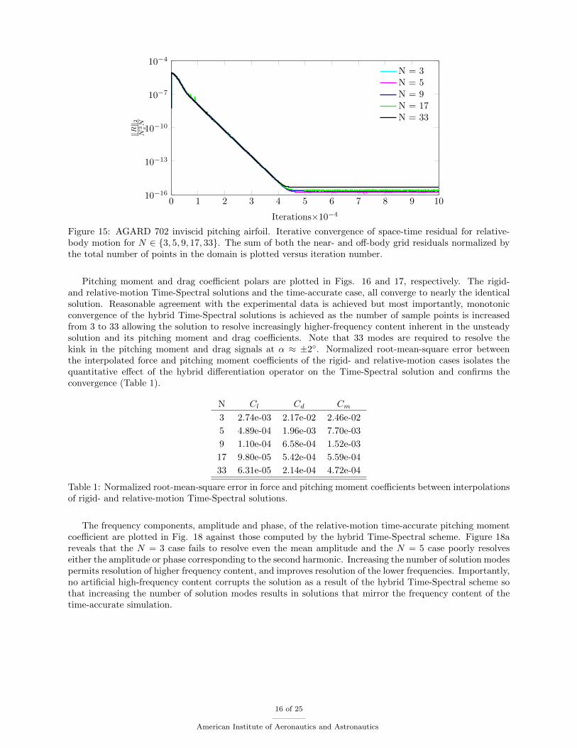
Figure 15: AGARD 702 inviscid pitching airfoil. Iterative convergence of space-time residual for relative-body motion for N ∈ {3, 5, 9, 17, 33}. The sum of both the near- and off-body grid residuals normalized bythe total number of points in the domain is plotted versus iteration number.

Pitching moment and drag coefficient polars are plotted in Figs. 16 and 17, respectively. The rigid-and relative-motion Time-Spectral solutions and the time-accurate case, all converge to nearly the identicalsolution. Reasonable agreement with the experimental data is achieved but most importantly, monotonicconvergence of the hybrid Time-Spectral solutions is achieved as the number of sample points is increasedfrom 3 to 33 allowing the solution to resolve increasingly higher-frequency content inherent in the unsteadysolution and its pitching moment and drag coefficients. Note that 33 modes are required to resolve thekink in the pitching moment and drag signals at α ≈ ±2◦. Normalized root-mean-square error betweenthe interpolated force and pitching moment coefficients of the rigid- and relative-motion cases isolates thequantitative effect of the hybrid differentiation operator on the Time-Spectral solution and confirms theconvergence (Table 1).

N Cl Cd Cm

3 2.74e-03 2.17e-02 2.46e-02

5 4.89e-04 1.96e-03 7.70e-03

9 1.10e-04 6.58e-04 1.52e-03

17 9.80e-05 5.42e-04 5.59e-04

33 6.31e-05 2.14e-04 4.72e-04

Table 1: Normalized root-mean-square error in force and pitching moment coefficients between interpolationsof rigid- and relative-motion Time-Spectral solutions.

The frequency components, amplitude and phase, of the relative-motion time-accurate pitching momentcoefficient are plotted in Fig. 18 against those computed by the hybrid Time-Spectral scheme. Figure 18areveals that the N = 3 case fails to resolve even the mean amplitude and the N = 5 case poorly resolveseither the amplitude or phase corresponding to the second harmonic. Increasing the number of solution modespermits resolution of higher frequency content, and improves resolution of the lower frequencies. Importantly,no artificial high-frequency content corrupts the solution as a result of the hybrid Time-Spectral scheme sothat increasing the number of solution modes results in solutions that mirror the frequency content of thetime-accurate simulation.

16 of 25


−3 −2 −1 0 1 2 3−2

−1

0

1

2

α

Cm×

102

Time AccurateRelative MotionRigid Motion

(a) N = 3

−3 −2 −1 0 1 2 3−2

−1

0

1

2

α

Cm×

102

(b) N = 9

−3 −2 −1 0 1 2 3−2

−1

0

1

2

α

Cm×

102

(c) N = 33

Figure 16: AGARD 702 inviscid pitching airfoil. Time Spectral versus Time Accurate pitching momentcoefficients for N ∈ {3, 9, 33}. Ten periods of the rigid-motion time-accurate solution are plotted in redfrom steady-state startup. Blue squares locate the pitching moment coefficient values at the Time-Spectralcollocation points for relative-body motion. Relative-body pitching moment coefficients computed from aninterpolation of the Time-Spectral solution to 201 points shown with the blue-hashed line. Green diamondslocate the pitching moment coefficient values at the Time-Spectral collocation points for rigid-body motion.Rigid-body pitching moment coefficients computed from an interpolation of the Time-Spectral solution to201 points shown with the green-hashed line. Experimental data from the AGARD 702 Report are plottedwith black dots. 17 of 25


−3 −2 −1 0 1 2 30

0.5

1

1.5

2

2.5

3

α

Cd×

102

Time AccurateRelative MotionRigid Motion

(a) N = 3

−3 −2 −1 0 1 2 30

0.5

1

1.5

2

2.5

3

α

Cd×

102

(b) N = 9

−3 −2 −1 0 1 2 30

0.5

1

1.5

2

2.5

3

α

Cd×

102

(c) N = 33

Figure 17: AGARD 702 inviscid pitching airfoil. Time Spectral versus Time Accurate drag coefficientsfor N ∈ {3, 9, 33}. Ten periods of the rigid-motion time-accurate solution are plotted in red from steady-state startup. Blue squares locate the drag coefficient values at the Time-Spectral collocation points forrelative-body motion. Relative-body drag coefficients computed from an interpolation of the Time-Spectralsolution to 201 points shown with the blue-hashed line. Green diamonds locate the drag coefficient valuesat the Time-Spectral collocation points for rigid-body motion. Rigid-body drag coefficients computed froman interpolation of the Time-Spectral solution to 201 points shown with the green-hashed line. Correctedexperimental drag data from the AGARD 702 Report are not available.

18 of 25


0 2 4 6 8 10 12 14 16 18 2010−7

10−6

10−5

10−4

10−3

10−2

f

<|Cm|

Time AccurateN = 3N = 5N = 9N = 17N = 33

(a) Amplitude, <|Cm|

0 2 4 6 8 10 12 14 16 18 2010−7

10−6

10−5

10−4

10−3

10−2

f

=|Cm|

(b) Phase, =|Cm|

Figure 18: AGARD 702 inviscid pitching airfoil. Spectra of time-accurate and Time-Spectral pitchingmoment coefficients, Cm = Φ−1Cm, for first 20 harmonics of the relative motion case. Increasing modalresolution results in better agreement between pitching moment amplitude and phase without introducingspurious high-frequency content.

Turbulent RANS Case

Practical applications of the Time-Spectral method including rotorcraft and turbomachinery involve turbu-lent flows, and therefore the previous oscillatory airfoil is extended to use the Spalart-Allmaras one-equationturbulence model. OVERFLOW employs a loosely coupled turbulence scheme whereby the turbulent vari-ables are updated initially and held constant for the flow-equation iteration. The code structure prevents adirect Time-Spectral implicit treatment for the turbulent variable without a significant overhaul. Instead, asemi-implicit treatment retroactively applies the implicit operator to the explicit turbulent update, ∆νn+

12 .

[I + ∆τAx] [I + ∆τAy] [I + ∆τAz] ∆νn+12 = −∆τ [R (νn) + S (νn)] (15)

19 of 25


νn+12 is then held fixed while iterating the flow solution, Q.

Qn+1 = Qn + ∆Q(νn+

12

)(16)

The implicit update ∆νn+1 is computed and retroactively applied to νn to advance the solution prior to thesubsequent time step.

[I + ∆τD] ∆νn+1 = ∆νn+12 (17)

Figure 19 shows contours of the (undamped) turbulent eddy viscosity, ν, in the wake region for the fivetemporal collocation points of the pitching airfoil. This illustrates the potentially large changes in ν as afunction of time in the wake region.

Figure 19: Visualization of undamped turbulent eddy viscosity on the near-body grid and in the wake regionof the AGARD 702 pitching airfoil at the temporal collocation points for a representative case of N = 5.ν can vary several orders of magnitude in a short time frame and must be limited in certain circumstancesto avoid spurious undershoots resulting from Gibbs’ phenomenon. The figure shows every second grid pointremoved in the normal direction for clarity.

Figure 20 plots the time history of turbulent eddy viscosity and its temporal derivative at a pointdownstream of the airfoil through which the turbulent wake passes during a portion of the oscillation. Notein Fig. 20a, the turbulent eddy viscosity transitions from a constant value of order zero to a value of order1000 over a small fraction of the period. While the function varies smoothly in the context of the smallphysical time steps associated with time-accurate iterations, it resembles a discontinuous step function inthe frame of the much coarser resolution of Time-Spectral sample points. This leads to spurious oscillationsin the Fourier expansion (Gibbs’ phenomenon). Oscillations in the gradient are manifested at the discretesample points which can be observed in Fig. 20b resulting in large overshoots. This issue is compoundedby the fact that undamped eddy viscosity remains close to zero outside the wake, so that modest overshootsin the derivative violate the positivity constraint on ν. The current example uses eddy viscosity in theSpalart-Allmaras model, however, similar issues are encountered for turbulent kinetic energy or dissipationin other models. The same phenomenon could also occur in the fluid equations for high-speed cases. Notethat this issue applies to Time-Spectral treatment of turbulence in general as it occurs downstream from thebody on nodes with complete time histories.

Applying a limiter to the temporal differentiation operator maintains positivity on ν without sacrificingaccuracy. The current limiter sets the Time-Spectral source term to zero if it would drive ν negative.Figure 20a demonstrates good agreement between the Time-Spectral and time-accurate solutions for ν atthe collocation points. Slight ringing does occur in the constant region but ν remains positive.

20 of 25


0 0.1 0.2 0.3 0.4 0.5 0.6 0.7 0.8 0.9 1−200

0

200

400

600

t∗/T

ν

Time AccurateFourier ExpansionTime Spectral

(a) Turbulent variable, ν (t)

0 0.1 0.2 0.3 0.4 0.5 0.6 0.7 0.8 0.9 1−200

−100

0

100

Gradient Limited Gradient Limited

t∗/T

∂ν∂t

(b) Time derivative, ∂ν∂t

(t)

Figure 20: AGARD 702 turbulent pitching airfoil. (a) Turbulent solution variable, ν (t), and (b) its derivative,∂ν∂t , are plotted for a point in the wake over the period of oscillation. BDF2 and Fourier operators differenti-ated the continuous and discrete data, respectively. Note, Gibbs’ phenomenon in the Fourier representationof the signal are present in the derivative where large oscillations lead to an inaccurate representation of ∂ν

∂t(t∗ = t− T/4).

Only the relative-motion Time-Spectral scheme is applied to the viscous case as the hybrid scheme alreadydemonstrated its ability to match the results computed with the conventional Time-Spectral scheme for theinviscid rigid-body case. The pitching moment and drag coefficients computed from the Time-Spectralsimulations converge to those computed in unsteady mode with increasing numbers of temporal collocationpoints (Figs. 21 and 22). Note that N = 33 modes are required to resolve the kink in the pitching momentand drag coefficient signals at α ≈ ±2◦ (Figs. 21c and 22c), as with the inviscid case. Less agreement isobserved with the experimental data in the pitching moment coefficient polars (Fig. 21) when comparedto the inviscid case from the previous section but this discrepancy also occurs in the time-accurate casesuggesting a physical modeling issue. While experimental data are included for reference, the crucial pointremains that the Time-Spectral results converge monotonically to those computed with the time-accuratesolver.

21 of 25


−3 −2 −1 0 1 2 3−2

−1

0

1

2

α

Cm×

102

Time AccurateRelative Motion

(a) N = 3

−3 −2 −1 0 1 2 3−2

−1

0

1

2

α

Cm×

102

(b) N = 9

−3 −2 −1 0 1 2 3−2

−1

0

1

2

α

Cm×

102

(c) N = 33

Figure 21: AGARD 702 turbulent pitching airfoil. Time Spectral versus Time Accurate pitching momentcoefficients for N ∈ {3, 9, 33}. Ten periods of the time-accurate solution are plotted in red from steady-statestartup. Blue squares locate the pitching moment coefficient values at the Time-Spectral collocation pointsfor relative-body motion. Relative-body motion pitching moment coefficients computed from an interpolationof the Time-Spectral solution to 201 points shown with the blue-hashed line. Experimental data from theAGARD 702 Report are plotted with black dots.

22 of 25


−3 −2 −1 0 1 2 30.25

0.75

1.25

1.75

2.25

α

Cd×

102

Time AccurateRelative Motion

(a) N = 3

−3 −2 −1 0 1 2 30.25

0.75

1.25

1.75

2.25

α

Cd×

102

(b) N = 9

−3 −2 −1 0 1 2 30.25

0.75

1.25

1.75

2.25

α

Cd×

102

(c) N = 33

Figure 22: AGARD 702 turbulent pitching airfoil. Time Spectral versus Time Accurate drag coefficients forN ∈ {3, 9, 33}. Ten periods of the time-accurate solution are plotted in red from steady-state startup. Bluesquares locate the drag coefficient values at the Time-Spectral collocation points for relative-body motion.Relative-body motion drag coefficients computed from an interpolation of the Time-Spectral solution to 201points shown with the blue-hashed line. Corrected experimental drag data from the AGARD 702 Reportare not available.

23 of 25


VI. Summary

A new hybrid Time-Spectral method has been introduced for dynamic overset and Cartesian applications.The time samples of spatial nodes that undergo dynamic blanking are segmented into intervals of consec-utively unblanked temporal collocation points and differentiated by an operator derived from barycentricrational interpolants. Barycentric rational interpolation offers superior approximation and differentiationproperties on an equispaced aperiodic mesh in contrast to traditional orthogonal polynomials. The majorityof nodes are unblanked and treated with the standard Time-Spectral formulation.

The hybrid scheme was outlined and evaluated with a linear model problem and the implementationof the hybrid Time-Spectral scheme within the NASA OVERFLOW solver was described. Inviscid andturbulent test cases of plunging and pitching airfoils solved using both rigid and relative motion agreed withtime-accurate solutions. The hybrid Time-Spectral scheme performed well in the inviscid subsonic plungingairfoil case where its conserved solution variables and drag coefficient values converged to the time-accuratedata. The AGARD 702 pitching airfoil case demonstrated temporal convergence in its pitching moment anddrag signals requiring N = 33 modes to resolve the finest details of the solution. Spectrum analysis confirmedthat no artificial high-frequency content was generated. A limiter was employed in the turbulent case toavoid large oscillations in the gradient of the turbulent eddy viscosity in the wake. Temporal convergencewas similarly observed for the viscous case. The hybrid Time-Spectral results matched those computed withthe conventional Time-Spectral approach and converged monotonically to the the time-accurate solutions,establishing the hybrid scheme as a viable tool for the simulation of periodically forced flows.

Future work includes acceleration of the code through multigrid and other techniques to enable applicationto more realistic problems in rotorcraft and turbomachinery. Dynamic near-body to near-body hole-cuttingoccurs in these problems and will therefore be investigated. Optimal selection of the rational interpolationapproximation order, d, and its maximum value, dmax, remains part of future work in addition to the stabilityanalysis for the rational-based differentiation operator.

Acknowledgments

The authors would like to thank the US Army Aeroflightdynamics Directorate (AMRDEC) for sponsoringthis research and the NASA Education Associates Program (EAP).

References

1Hall, K., Thomas, J., and Clark, W., “Computation of Unsteady Nonlinear Flows in Cascades using a Harmonic BalanceTechnique,” 9th International Symposium on Unsteady Aerodynamics, Aeroacoustics and Aeroelasticity of Turbomachines,Lyon, France, September 2000.

2Hall, K., Thomas, J., and Clark, W., “Computation of Unsteady Nonlinear Flows in Cascades Using a Harmonic BalanceTechnique,” AIAA Journal , Vol. 40, May 2002, pp. 879–886.

3McMullen, M. S. and Jameson, A., “The Computational Efficiency of Non-Linear Frequency Domain Methods,” Journalof Computational Physics, Vol. 212, 2006, pp. 637–661.

4McMullen, M., Jameson, A., and Alonso, J., “Demonstration of Nonlinear Frequency Domain Methods,” AIAA Journal ,Vol. 44, No. 7, July 2006, pp. 1428–1435.

5Nadarajah, S. K., McMullen, M. S., and Jameson, A., “Optimum Shape Design for Unsteady Flow Using Time Accurateand Non-Linear Frequency Domain Methods,” AIAA Paper 3875, June 2003.

6Murman, S. M., “A Reduced-Frequency Approach for Calculating Dynamic Derivatives,” AIAA Journal , Vol. 45, No. 6,June 2007, pp. 1161–1168.

7Gopinath, A. K. and Jameson, A., “Time Spectral Method for Periodic Unsteady Computations over Two- and Three-Dimensional Bodies,” AIAA Paper 1220, January 2005.

8Gopinath, A. K. and Jameson, A., “Application of the Time Spectral Method to Periodic Vortex Shedding,” AIAA Paper0449, January 2006.

9Blanc, F., Roux, F.-X., Jouhaud, J.-C., and Boussuge, J.-F., “Numerical Methods for Control Surfaces Aerodynamicswith Flexibility Effects,” IFASD 2009, Seattle, WA, June 2009.

10Choi, S., Potsdam, M., Lee, K., Iaccarino, G., and Alonso, J. J., “Helicopter Rotor Design Using a Time-Spectral andAdjoint-Based Method,” AIAA Paper 5810, September 2008.

11Nadarajah, S. K. and Tatossian, C. A., “Adjoint-Based Aerodynamic Shape Optimization of Rotorcraft Blades,” AIAAPaper 6730, August 2008.

12Mosahebi, A. and Nadarajah, S. K., “An Implicit Adaptive Non-Linear Frequency Domain Method (pNLFD) for ViscousPeriodic Steady State Flows on Deformable Grids,” AIAA Paper 0775, January 2011.

13Maple, R. C., King, P. I., Wolff, J. M., and Orkwis, P. D., “Split-Domain Harmonic Balance Solutions to Burger’sEquation for Large-Amplitude Distrubances,” AIAA Journal , Vol. 41, No. 2, February 2003, pp. 206–212.

24 of 25


14Maple, R. C., King, P. I., and Oxley, M. E., “Adaptive Harmonic Balance Solutions to Euler’s Equation,” AIAA Journal ,Vol. 41, No. 9, September 2003, pp. 1705–1714.

15Thomas, J. P., Custer, C. H., Dowell, E. H., and Hall, K. C., “Unsteady Flow Computation Using a Harmonic BalanceApproach Implemented about the OVERFLOW 2 Flow Solver,” AIAA Paper 4270, June 2009.

16Custer, C. H., A Nonlinear Harmonic Balance Solver for an Implicit CFD Code: OVERFLOW 2 , Ph.D. thesis, DukeUniversity, 2009.

17Mavriplis, D., Yang, Z., and Mundis, N., “Extensions of Time Spectral Methods for Practical Rotorcraft Problems,”AIAA Paper 0423, January 2012.

18Strang, G., “The Optimal Coefficients in Daubechies Wavelets,” Physica D , Vol. 60, 1992, pp. 239–244.19Romine, C. H. and Peyton, B. W., “Computing Connection Coefficients of Compactly Supported Wavelets on Bounded

Intervals,” Mathematical Sciences Section ORNL/TM-13413, Oak Ridge National Laboratory, April 1997.20Huybrechs, D., “On the Fourier Extension of Nonperiodic Functions,” SIAM Journal of Numerical Analysis, Vol. 47,

No. 6, 2010, pp. 4326–4355.21Boyd, J. P., “A Comparison of Numerical Algorithms for Fourier Extension of the First, Second, and Third Kinds,”

Journal of Computational Physics, Vol. 178, 2002, pp. 118–160.22Bruno, O. P., Han, Y., and Pohlman, M. M., “Accurate, High-Order Representation of Complex Three-Dimensional

Surfaces via Fourier Continuation Analysis,” Journal of Computational Physics, Vol. 227, 2007, pp. 1094–1125.23Candes, E., “Compressive Sampling,” International Congress of Mathematicians, Madrid, Spain, 2006.24Platte, R. B., Trefethen, L. N., and Kuijlaars, A. B., “Impossibility of Fast Stable Approximation of Analytic Functions

from Equispaced Samples,” SIAM Review , Vol. 53, No. 2, 2011, pp. 308–318.25Bos, L., De Marchi, S., Hormann, K., and Klein, G., “On the Lebesgue Constant of Barycentric Rational Interpolation

at Equidistant Nodes,” Numerische Mathematik , Vol. 121, No. 3, 2012, pp. 461–471.26Baltensperger, R. and Berrut, J.-P., “The Linear Rational Collocation Method,” Journal of Computational and Applied

Mathematics, Vol. 134, 2001, pp. 243–258.27Berrut, J.-P. and Baltensperger, R., “The Linear Rational Pseudospectral Method for Boundary Value Problems,” BIT ,

Vol. 41, No. 5, 2001, pp. 868–879.28Klein, G., “An Extension of the Floater-Hormann Family of Barycentric Rational Interpolants,” Mathematics of Com-

putation, accepted for publication.29Tee, T. W. and Trefethen, L. N., “A Rational Spectral Collocation Method with Adaptively Transformed Chebyshev

Grid Points,” SIAM Journal of Scientific Computing, Vol. 28, No. 5, 2006, pp. 1798–1811.30Baltensperger, R., Berrut, J.-P., and Noel, B., “Exponential Convergence of a Linear Rational Interpolant Between

Transformed Chebyshev Points,” Mathematics of Computation, Vol. 68, No. 227, 1999, pp. 1109–1120.31Floater, M. S. and Hormann, K., “Barycentric Rational Interpolation with No Poles and High Rates of Approximation,”

Numerische Mathematik , Vol. 107, No. 2, August 2007, pp. 315–331.32Wang, Q., Moin, P., and Iaccarino, G., “A Rational Interpolation Scheme with Superpolynomial Rate of Convergence,”

SIAM Journal of Numerical Analysis, Vol. 47, No. 6, 2010, pp. 4073–4097.33Nichols, R. and Buning, P., “Solver and Turbulence Model Upgrades to OVERFLOW 2 for Unsteady and High-Speed

Applications,” AIAA Paper 2824, 2006.34Landon, R. H., “Compendium of Unsteady Aerodynamic Measurements,” AGARD Report No. 702, August 1982.

25 of 25


51st aiaa aerospace sciences meeting including the new ... · 51st aiaa aerospace sciences meeting...

Documents