44086-chapter 1

8/8/2019 44086-Chapter 1

http://slidepdf.com/reader/full/44086-chapter-1 1/12

Chapter 1

1.1

(a) One dimensional, multichannel, discrete time, and digital.(b) Multi dimensional, single channel, continuous-time, analog.(c) One dimensional, single channel, continuous-time, analog.(d) One dimensional, single channel, continuous-time, analog.(e) One dimensional, multichannel, discrete-time, digital.

1.2

(a) f = 0.01π2π

= 1200⇒ periodic with N p = 200.

(b) f = 30π105 ( 1

2π ) = 17 ⇒ periodic with N p = 7.

(c) f = 3π2π

= 32 ⇒ periodic with N p = 2.

(d) f = 32π⇒ non-periodic.

(e) f = 62π10

( 12π

) = 3110 ⇒ periodic with N p = 10.

1.3

(a) Periodic with period T p = 2π5 .

(b) f = 52π ⇒ non-periodic.

(c) f = 112π ⇒ non-periodic.(d) cos(n8 ) is non-periodic; cos(πn8 ) is periodic; Their product is non-periodic.(e) cos(πn

2) is periodic with period N p=4

sin(πn8

) is periodic with period N p=16cos(πn

4+ π

3) is periodic with period N p=8

Therefore, x(n) is periodic with period N p=16. (16 is the least common multiple of 4,8,16).

1.4

(a) w = 2πkN

implies that f = kN

. Let

α = GCD of (k, N ), i.e.,

k = k′α,N = N ′α.

Then,

f =k′

N ′, which implies that

N ′ =N

α.

3

© 2007 Pearson Education, Inc., Upper Saddle River, NJ. All rights reserved. This material is protected under all copyright laws

as they currently exist. No portion of this material may be reproduced, in any form or by any means, without permission in

writing from the publisher. For the exclusive use of adopters of the book Digital Signal Processing, Fourth Edition, by John G.

Proakis and Dimitris G. Manolakis. ISBN 0-13-187374-1.

8/8/2019 44086-Chapter 1


(b)

N = 7

k = 0 1 2 3 4 5 6 7

GCD(k, N ) = 7 1 1 1 1 1 1 7

N p = 1 7 7 7 7 7 7 1

(c)

N = 16

k = 0 1 2 3 4 5 6 7 8 9 10 11 12 . . . 16

GCD(k, N ) = 16 1 2 1 4 1 2 1 8 1 2 1 4 . . . 16

N p = 1 6 8 16 4 16 8 16 2 16 8 16 4 . . . 1

1.5

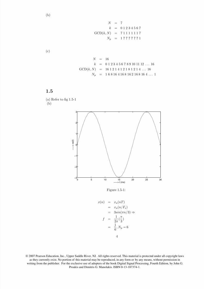
(a) Refer to fig 1.5-1(b)

0 5 10 15 20 25 30−3

−2

−1

0

1

2

3

−−−> t (ms)

− − − >

x a ( t )

Figure 1.5-1:

x(n) = xa(nT )= xa(n/F s)

= 3sin(πn/3) ⇒

f =1

2π(π

3)

=1

6, N p = 6

4





8/8/2019 44086-Chapter 1


0 10 20t (ms)

3

-3

Figure 1.5-2:

(c)Refer to fig 1.5-2

x(n) =

0, 3√ 2, 3√

2, 0,− 3√

2,− 3√

2

,N p = 6.

(d) Yes.

x(1) = 3 = 3sin(100π

F s) ⇒ F s = 200 samples/sec.

1.6

(a)

x(n) = Acos(2πF 0n/F s + θ)

= Acos(2π(T/T p)n + θ)

But T/T p = f ⇒ x(n) is periodic if f is rational.(b) If x(n) is periodic, then f=k/N where N is the period. Then,

T d = (k

f T ) = k(

T pT

)T = kT p.

Thus, it takes k periods (kT p) of the analog signal to make 1 period (T d) of the discrete signal.(c) T d = kT p ⇒ NT = kT p ⇒ f = k/N = T/T p ⇒ f is rational ⇒ x(n) is periodic.

1.7

(a) F max = 10kHz ⇒ F s ≥ 2F max = 20kHz.

(b) For F s = 8kHz,F fold = F s/2 = 4kHz ⇒ 5kHz will alias to 3kHz.(c) F=9kHz will alias to 1kHz.

1.8

(a) F max = 100kHz,F s ≥ 2F max = 200Hz.(b) F fold = F

s

2= 125Hz.

5





8/8/2019 44086-Chapter 1


1.9

(a) F max = 360Hz,F N = 2F max = 720Hz.(b) F fold = F

s

2= 300Hz.

(c)

x(n) = xa(nT )

= xa(n/F s)

= sin(480πn/600) + 3sin(720πn/600)

x(n) = sin(4πn/5)− 3sin(4πn/5)

= −2sin(4πn/5).

Therefore, w = 4π/5.(d) ya(t) = x(F st) = −2sin(480πt).

1.10

(a)

Number of bits/sample = log21024 = 10.

F s =[10, 000 bits/sec]

[10 bits/sample]

= 1000 samples/sec.

F fold = 500Hz.

(b)

F max =1800π

2π= 900Hz

F N = 2F max = 1800Hz.

(c)

f 1 =600π

2π(

1

F s)

= 0.3;

f 2 =1800π

2π(

1

F s)

= 0.9;

But f 2 = 0.9 > 0.5 ⇒ f 2 = 0.1.

Hence, x(n) = 3cos[(2π)(0.3)n] + 2cos[(2π)(0.1)n]

(d) △ =xmax−xmin

m−1= 5−(−5)

1023= 10

1023.

1.11

x(n) = xa(nT )

= 3cos

100πn

200

+ 2sin

250πn

200

6





8/8/2019 44086-Chapter 1


= 3cosπn

2

− 2sin

3πn

4

T ′ =1

1000⇒ ya(t) = x(t/T ′)

= 3cos

π1000t

2

− 2sin

3π1000t

4

ya(t) = 3cos(500πt)− 2sin(750πt)

1.12

(a) For F s = 300Hz,

x(n) = 3cosπn

6

+ 10sin(πn)− cos

πn3

= 3cosπn

6

− 3cos

πn3

(b) xr(t) = 3cos(10000πt/6)− cos(10000πt/3)

1.13

(a)

Range = xmax − xmin = 12.7.

m = 1 +range

△

= 127 + 1 = 128 ⇒ log2(128)

= 7 bits.

(b) m = 1 + 1270.02 = 636 ⇒ log2(636) ⇒ 10 bit A/D.

1.14

R = (20samples

sec)× (8

bits

sample)

= 160bits

sec

F fold =F s2

= 10Hz.

Resolution =1volt

28 − 1= 0.004.

1.15

(a) Refer to fig 1.15-1. With a sampling frequency of 5kHz, the maximum frequency that can berepresented is 2.5kHz. Therefore, a frequency of 4.5kHz is aliased to 500Hz and the frequency of 3kHz is aliased to 2kHz.

7





8/8/2019 44086-Chapter 1


0 50 100−1

−0.5

0

0.5

1Fs = 5KHz, F0=500Hz

0 50 100−1

−0.5

0

0.5

1Fs = 5KHz, F0=2000Hz

0 50 100−1

−0.5

0

0.5

1Fs = 5KHz, F0=3000Hz

0 50 100−1

−0.5

0

0.5

1Fs = 5KHz, F0=4500Hz

Figure 1.15-1:

(b) Refer to fig 1.15-2. y(n) is a sinusoidal signal. By taking the even numbered samples, thesampling frequency is reduced to half i.e., 25kHz which is still greater than the nyquist rate. Thefrequency of the downsampled signal is 2kHz.

1.16

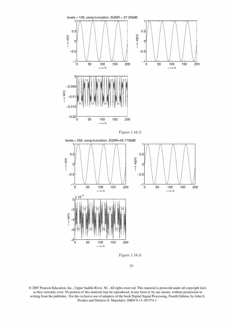
(a) for levels = 64, using truncation refer to fig 1.16-1.for levels = 128, using truncation refer to fig 1.16-2.for levels = 256, using truncation refer to fig 1.16-3.

8





8/8/2019 44086-Chapter 1


0 10 20 30 40 50 60 70 80 90 100−1

−0.5

0

0.5

1F0 = 2KHz, Fs=50kHz

0 5 10 15 20 25 30 35 40 45 50−1

−0.5

0

0.5

1F0 = 2KHz, Fs=25kHz

Figure 1.15-2:

0 50 100 150 200−1

−0.5

0

0.5

1levels = 64, using truncation, SQNR = 31.3341dB

−−> n

− − >

x ( n )

0 50 100 150 200−1

−0.5

0

0.5

1

−−> n

− − >

x q ( n )

0 50 100 150 200−0.04

−0.03

−0.02

−0.01

0

−−> n

− − >

e ( n )

Figure 1.16-1:

9





8/8/2019 44086-Chapter 1


0 50 100 150 200−1

−0.5

0

0.5

1levels = 128, using truncation, SQNR = 37.359dB

−−> n

− − >

x ( n )

0 50 100 150 200−1

−0.5

0

0.5

1

−−> n

− − >

x q ( n )

0 50 100 150 200−0.02

−0.015

−0.01

−0.005

0

−−> n

− − > e

( n )

Figure 1.16-2:

0 50 100 150 200−1

−0.5

0

0.5

1levels = 256, using truncation, SQNR=43.7739dB

−−> n

− − >

x ( n )

0 50 100 150 200−1

−0.5

0

0.5

1

−−> n

−

− >

x q ( n )

0 50 100 150 200−8

−6

−4

−2

0x 10

−3

−−> n

− − >

e ( n )

Figure 1.16-3:

10





8/8/2019 44086-Chapter 1


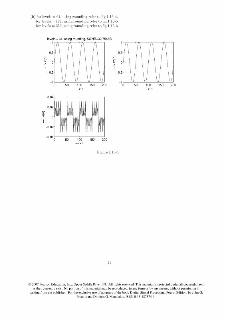
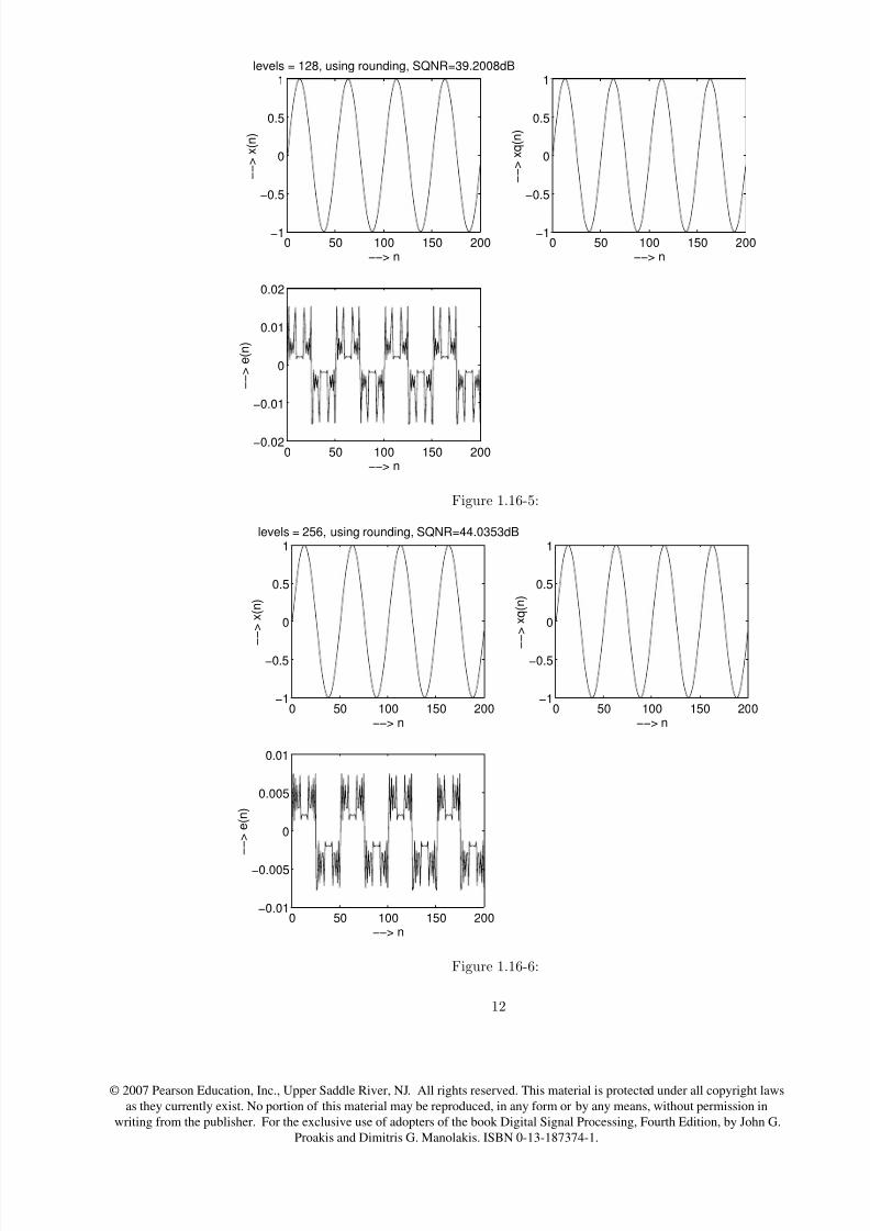
(b) for levels = 64, using rounding refer to fig 1.16-4.for levels = 128, using rounding refer to fig 1.16-5.for levels = 256, using rounding refer to fig 1.16-6.

0 50 100 150 200−1

−0.5

0

0.5

1levels = 64, using rounding, SQNR=32.754dB

−−> n

− − >

x ( n )

0 50 100 150 200−1

−0.5

0

0.5

1

−−> n

− − > x

q ( n )

0 50 100 150 200−0.04

−0.02

0

0.02

0.04

−−> n

− − >

e ( n

)

Figure 1.16-4:

11





8/8/2019 44086-Chapter 1


0 50 100 150 200−1

−0.5

0

0.5


−−> n

− − >

x ( n )

0 50 100 150 200−1

−0.5

0

0.5

1

−−> n

− − >

x q ( n )

0 50 100 150 200−0.02

−0.01

0

0.01

0.02

−−> n

− − >

e ( n )

Figure 1.16-5:

0 50 100 150 200−1

−0.5

0

0.5


−−> n

− − >

x ( n )

0 50 100 150 200−1

−0.5

0

0.5

1

−−> n

−

− >

x q ( n )

0 50 100 150 200−0.01

−0.005

0

0.005

0.01

−−> n

− − >

e ( n )

Figure 1.16-6:

12





8/8/2019 44086-Chapter 1


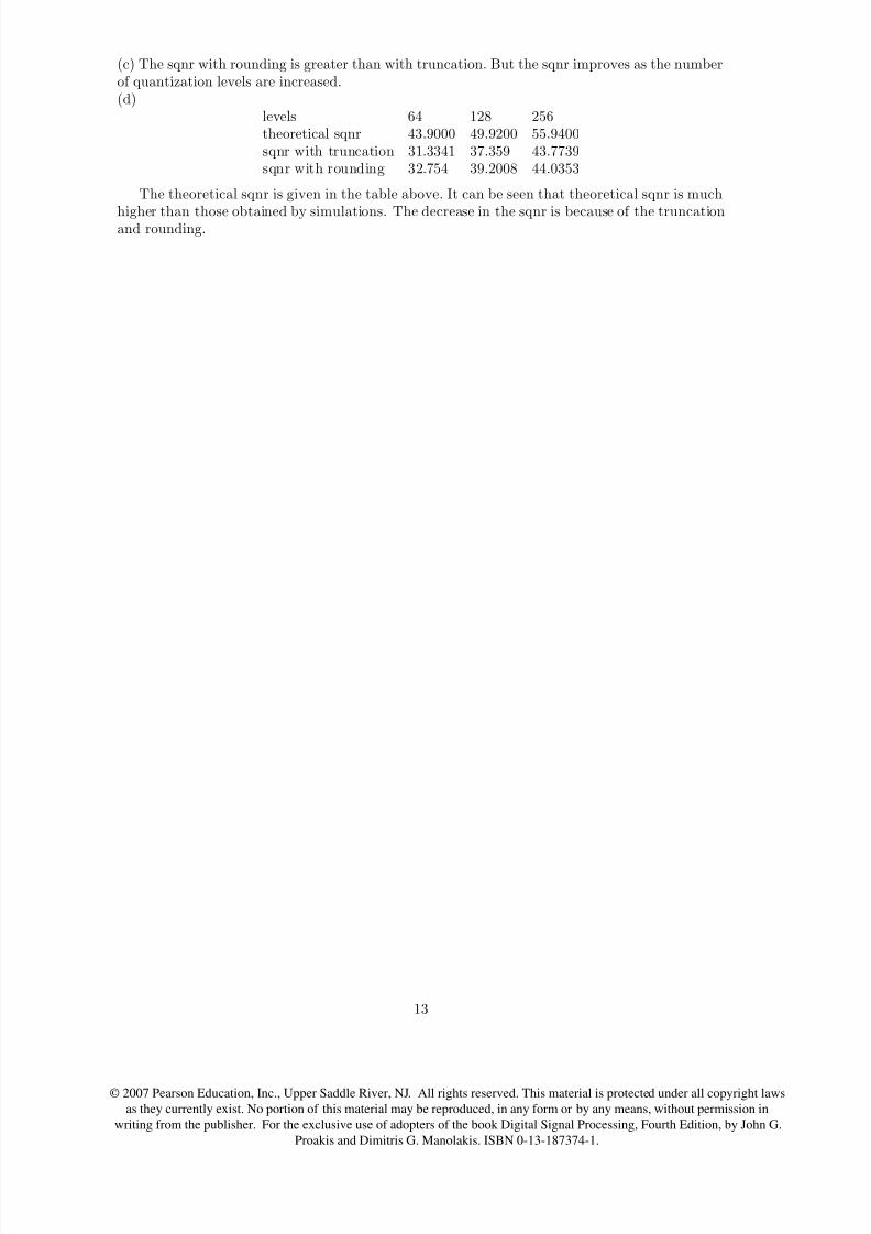
(c) The sqnr with rounding is greater than with truncation. But the sqnr improves as the numberof quantization levels are increased.(d)

levels 64 128 256theoretical sqnr 43.9000 49.9200 55.9400sqnr with truncation 31.3341 37.359 43.7739sqnr with rounding 32.754 39.2008 44.0353

The theoretical sqnr is given in the table above. It can be seen that theoretical sqnr is much

higher than those obtained by simulations. The decrease in the sqnr is because of the truncationand rounding.

13





8/8/2019 44086-Chapter 1


14





44086-chapter 1

Documents