3 repeated measures analysis of variance - stat.ncsu.edudavidian/st732/notes/chap3.pdf · 3.2...

CHAPTER 3 LONGITUDINAL DATA ANALYSIS

3 Repeated Measures Analysis of Variance

3.1 Introduction

As we have discussed, many approaches have been taken in the literature to specifying statistical

models for longitudinal data. Within the framework of a specific model, the questions of scien-

tific interest are interpreted and represented formally, and associated with the model are statistical

methods that allow the questions to be addressed. Different models embodying different assump-

tions and taking different perspectives (e.g., SS vs. PA) lead to possibly different characterizations of

the questions and different methods.

We begin our review of approaches by considering two statistical models that form the basis for what

we have called classical methods. These methods are appropriate for continuous outcome or

outcomes that can be viewed as approximately continuous and that are reasonably thought to be

approximately normally distributed.

The models have several limitations relative to those underlying the more modern approaches that

we discuss in subsequent chapters.

• The models are really only applicable in the case of balanced data; that is, where the responses

on each individual are recorded at the same time points , with no departures from these times

or missing data. Thus, in this chapter, we assume that each individual is observed at the same

n time points t1, ... , tj , say, and each has an associated n-dimensional response vector, where

the j th element corresponds to the response at time tj .

• The models adopt a representation of the overall population mean of a response vector that is

simplistic in the sense that it does not recognize the fact that the mean response might exhibit

a systematic trajectory over continuous time, such as a straight line. In particular, the mean

ordinarily is represented using the notation that is commonplace when developing analysis of

variance methods. Time and among-individual covariates are viewed as categorical factors

with a small number of levels. The treatment of time as a categorical factor is particularly

restrictive.

64


• The models do not accommodate straightforwardly incorporation of covariate information be-

yond time and among-individual categorical factors. In our discussion, we restrict attention to a

single among-individual factor such as group membership ; e.g., gender in the dental study

or dose in the guinea pig diet study in EXAMPLE 2 of Section 1.2. Although the models can be

generalized to more than one such factor (e.g., genotype and weather pattern in the soybean

growth study of EXAMPLE 3 of Section 1.2), we do not consider this, deferring to the more

modern approaches we discuss later that allow much greater flexibility.

• The associated analysis methods are focused almost entirely on hypothesis testing. Thus,

they do not readily accommodate questions regarding the nature of features of mean trajec-

tories; e.g., in the dental study, the values of the slopes characterizing rate of change of

assumed straight line population mean trajectories for boys and girls. That is, estimation of

quantities like these is not straightforward within these modeling frameworks.

As we demonstrate, the models also embody assumptions on the overall covariance structure of a

response vector that are possibly too restrictive or too general.

• The statistical model underlying univariate repeated measures analysis of variance (ANOVA)

methods is derived from a SS perspective. As we noted in Section 2.5, it induces a model for

the overall covariance pattern that has a compound symmetric correlation structure, which

may or may not be a plausible model.

• The statistical model underlying multivariate repeated measures analysis of variance meth-

ods arises from PA perspective. No specific systematic assumption is made on the overall

covariance pattern, so that it is regarded as completely unstructured. If correlation does

exhibit a simpler pattern, these methods could be inefficient.

We first review the univariate methods, followed by the multivariate approach. Our discussion is

limited to the basic elements and thus is not meant to be comprehensive. Rather, it is meant only

to provide an appreciation of why statistical practice has moved toward favoring the modern methods

discussed in subsequent chapters. Accordingly, we simply present results and do not offer detailed

derivations or proofs.

65


3.2 Univariate repeated measures analysis of variance

We first discuss the basic model underlying univariate repeated measures ANOVA methods in the

classical notation. In particular, we present the usual “one way” model, where there is a single

among-individual factor such as gender in the dental study of EXAMPLE 1 of Section 1.2 or vitamin

E dose level in the guinea pig growth study of EXAMPLE 2.

BASIC SET-UP:

• The model assumes that the data arise from a study in which individuals are randomized or

naturally belong to one of g ≥ 1 groups; the group variable is often referred to as the between-

or among-units factor. Thus, in the dental study, g = 2 genders; in the guinea pig growth study,

g = 3 dose groups.

From the point of view of the general notation introduced in Section 2.2, the model thus accom-

modates a single scalar, categorical among-individual covariate with g possible values. The

model does not allow for within-individual covariates.

• The response is recorded on each of n occasions or under each of n conditions. In a longitudinal

study, this is usually “time ” but could be another repeated measurement condition. E.g., if men

are randomized into two groups, regular and modified diet, the response might be maximum

heart rate after separate occasions during which each spent 10, 20, 30, 45, and 60 minutes

walking on a treadmill. We use the generic term time ; this factor is often referred to in the

classical literature as the within-units factor. In the dental study, this is age (n = 4); in the

guinea pig study, weeks (n = 6).

Thus, from the point of view of the conceptual framework discussed in Section 2.3, the model

does not acknowledge explicitly that there is an underlying process in continuous time and

that there could be values of the response at times other than these n occasions.

• As noted above, we consider only the case where there is a single group factor. However, it

is is straightforward to extend the development to the case where the groups are determined by

a factorial design ; e.g. if in the guinea pig study there had been g = 6 groups, determined by

the factorial arrangement of 3 doses and 2 genders.

66


NOTATION AND MODEL: We present the model first using the classical notation and then demon-

strate how it can be expressed in the notation introduced in Chapter 2. Define

Yh`j = response on individual h in the `th group at time j .

• h = 1, ... , r`, where r` denotes the number of units in group `. Thus, in this notation, h indexes

units within a particular group; ` = 1, ... , g indexes groups; and j = 1, ... , n indexes the levels of

time. Note then that a specific individual is uniquely identified by the indices (h, `).

• The total number of individuals is m =g∑`=1

r`. Each is observed at n time points.

The classical model for Yh`j is then given by

Yh`j = µ + τ` + bh` + γj + (τγ)`j + eh`j . (3.1)

In the usual terminology accompanying classical ANOVA methods

• µ is an “overall mean,” τ` is the fixed deviation from the overall mean associated with being

in group `, γj is the fixed deviation associated with time j , and (τγ)`j is an additional fixed

deviation associated with group ` and time j ; that is, (τγ)`j is the interaction effect for group `

and time j .

• Thus, as we demonstrate explicitly below, the overall population mean response for the `th

group at time j is represented as

µ + τ` + γj + (τγ)`j .

• bh` is a random effect assumed to be independent of the among-individual covariate group

with conditional (on group) mean equal to the unconditional mean E(bh`) = 0 characterizing

how the “inherent mean ” for the hth individual in group ` deviates from the overall population

mean. Thus, (3.1) represents the inherent (conditional) mean for individual (h, `) as

µ + τ` + γj + (τγ)`j + bh`, (3.2)

and bh` characterizes among-individual behavior.

• eh`j is a within-individual deviation representing the net effect of realizations and measure-

ment error, independent of the among-individual covariate group, with conditional (on group)

mean equal to the unconditional mean E(eh`j ) = 0. This is often called the “random error ,” but

as we have remarked previously we prefer the term within-individual deviation to reflect the

fact that it embodies more than just measurement error.

67


Some observations are immediate.

• Model (3.1) has the same form as the statistical model for observations arising from an exper-

iment conducted according to a split plot design. Thus, as we show shortly, the analysis is

identical to that of a split plot experiment; however, the interpretation and further analyses

are different.

• The actual values of the times (e.g. ages 8, 10, 12, 14 in the dental study) do not appear

explicitly in the model. Rather, a separate deviation parameter γj and interaction parameter

(τγ)`j is associated with each time. Thus, the model takes no account of where the times of

observation are temporally; e.g. are they equally-spaced ?

Because (3.1) is a linear model , as discussed in Section 2.4, we can view it as a SS or PA model.

• From a SS perspective, as in (3.2),

µ + τ` + γj + (τγ)`j + bh`

represents the inherent mean trend for the hth individual in group ` at time j . Note this assumes

that the inherent mean for a given individual (h, `) deviates from the overall population mean by

the same amount, bh`, at each time j . Thus, this model implies that if an individual is “high”

relative to the overall mean response at time j , the individual is “high” at all other times.

This is often not a reasonable assumption. For example, consider the the conceptual represen-

tation in Figure 2.2. This assumption might be reasonable for the two uppermost individuals in

panel (b), as the “inherent trends” for these are roughly parallel to the overall mean response

trajectory. However, it is clearly not appropriate for the lowermost unit.

• Taking a PA perspective, write (3.1) as

Yh`j = µ + τ` + γj + (τγ)`j︸︷︷︸µ`j

+ bh` + eh`j︸︷︷︸εh`j

. (3.3)

In (3.3), εh`j = bh` + eh`j is the overall deviation reflecting aggregate deviation from this mean

due to among- and within-individual sources.

68


Because bh` and eh`j have mean 0 (conditional on the among-individual covariate group and

unconditionally), it follows that

E(Yh`j ) = µ`j = µ + τ` + γj + (τγ)`j ,

the overall population mean for the `th group at the jth time.

CONVENTION: Henceforth, we writeN (µ,σ2) to denote a univariate normal distribution with mean

µ and variance σ2. We write N (µ, V ) to denote a multivariate normal distribution with mean vector

µ and covariance matrix V . The meaning (univariate or multivariate) is ordinarily clear from the

context.

NORMALITY AND INDEPENDENCE ASSUMPTIONS: The model is completed by standard as-

sumptions on the random deviations bh` and eh`j , which lead to an assumption on the form of the

overall pattern of variance and correlation.

• bh` ∼ N (0,σ2b) and are independent for all h and `, so that where any individual “sits” in the

population is unrelated to where others “sit.” The fact that this normal distribution is identical

for ` = 1, ... , g reflects the assumption that bh` is independent of the among-individual covariate

group, so that among-individual variation is the same in all g populations. The variance

component σ2b represents the common magnitude of among-individual variation.

• eh`j ∼ N (0,σ2e) and are independent for all h, `, and j . As for bh`, that this normal distribution is

the same for ` = 1, ... , 1 follows from the assumption that the eh`j are independent of the among-

individual covariate group. Moreover, it also reflects the assumption that within-individual

variation is the same at all observation times. Independence across j also implies that within-

individual correlation across the observation times is negligible. The variance component

σ2e represents the magnitude of within-individual variation aggregated from all within-individual

sources, namely, the realization process and measurement error.

• The bh` and eh`j are assumed to be mutually independent for all h, `, and j . From the con-

ceptual representation point of view, this says that deviations due to within-individual sources

are of similar magnitude regardless of the magnitudes of the deviations bh` associated with the

units on which the observations are made. This is often reasonable; however, as we will see

later in the course, there are situations where it may not be reasonable.

69


VECTOR REPRESENTATION AND OVERALL COVARIANCE MATRIX: We can summarize the

model for the responses for individual (h, `) in the (n × 1) random vectorYh`1

Yh`2...

Yh`n

=

µ + τ` + γ1 + (τγ)`1

µ + τ` + γ2 + (τγ)`2...

µ + τ` + γn + (τγ)`n

+

bh`

bh`...

bh`

+

eh`1

eh`2...

eh`n

=

µ`1

µ`2...

µ`n

+

εh`1

εh`2...

εh`n

. (3.4)

With 1 a (n × 1) vector of 1s, we write (3.4) compactly as

Y h` = µ` + 1bh` + eh` = µ` + εh`. (3.5)

Under the foregoing assumptions, it is clear that each Yh`j is normally distributed with

E(Yh`j ) = µ`j = µ + τ` + γj + (τγ)`j , so that E(Y h`) = µ`,

var(Yh`j ) = var(bh`) + var(eh`j ) + 2cov(bh`, eh`j ) = σ2b + σ2

e.

(conditionally and unconditionally). Moreover, it is straightforward to show (try it) that

cov(Yh`j , Yh′`′j ′) = cov(εh`j , εh′`′j ′) = 0, h 6= h′,

where ` 6= `′ or ` = `′ and j 6= j ′ or j = j ′; i.e., the covariance between observations from two different

units from the same or different groups at the same or different times is zero, which implies under

normality that Yh`j and Yh′`′j ′ are independent.

Thus, under the assumptions of the model, for ` 6= `′ or ` = `′, the random vectors Y h` and Y h′`′

are independent, showing that the model automatically induces the usual assumption that data

vectors from different individuals are independent.

It is also straightforward to derive that

cov(Yh`j , Yh`j ′) = cov(εh`j , εh`′j ′) = E{(Yh`j − µ`j )(Yh`j ′ − µ`j ′)} = E{(bh` + eh`j )(bh` + eh`j ′)}

= E(bh`bh`) + E(eh`jbh`) + E(bh`eh`j ′) + E(eh`jeh`j ′) = σ2b.

Summarizing, we have that the m data vectors Y h`, h = 1, ... , r`, ` = 1, ... , g are all independent and

multivariate normal; that is, Y h` ∼ Nn(µ`, V ), where

V = var(Y h`) = var(εh`) =

σ2

b + σ2e σ2

b · · · σ2b

σ2b σ2

b + σ2e · · · σ2

b...

......

...

σ2b σ2

b · · · σ2b + σ2

e

. (3.6)

70


• This result follows directly from (3.5). Using the independence of bh` and eh`,

var(Y h`) = var(εh`) = var(1bh`) + var(eh`) = var(bh`)11′ + var(eh`),

which, writing

11′ = Jn =

1 · · · 1

1 · · · 1...

......

1 · · · 1

and var(eh`) = σ2eIn,

yields

var(Y h`) = var(εh`) = σ2bJn + σ2

eIn = V , (3.7)

where (3.7) is a compact expression for (3.6).

• From (3.6),

corr(Yh`j , Yh`j ′) =σ2

b

σ2b + σ2

e, j 6= j ′. (3.8)

Thus, the overall correlation between any two observations in Y h` is the same and equal to

(3.8). The quantity (3.8) is called the intraclass correlation in some contexts.

• These results show that the model assumes that the overall aggregate pattern of correlation

is compound symmetric or exchangeable. Note that, automatically, the correlation between

any two observations in Y h` is assumed to be positive, as ordinarily σ2b > 0 and σ2

e > 0.

• The model also assumes that var(Yh`j ) is constant for all j , so that overall variance does not

change over time.

• Finally, (3.6) shows that the model implies that var(Y h`) is assumed to be the same for all

groups ` = 1, ... , g, which reflects the assumed independence of bh` and eh` from the among-

individual covariate group.

RESULT: This modeling approach and its assumptions induce a compound symmetric model for

the overall aggregate pattern of correlation that is the same in each group. As we have noted pre-

viously, the compound symmetric model can be a restrictive representation of the overall pattern of

correlation in the case within-individual sources of correlation are nonnegligible. The compound

symmetric structure emphasizes among-individual sources of correlation, so may be reasonable

when these sources are dominant.

71


The approach also induces the restriction that overall variance is constant across observation

times. This is may not always be a realistic assumption for longitudinal data, as in many settings

overall variance exhibits an increasing pattern over time.

Historically, the analysis methods we discuss shortly that are associated with this model have been

used widely in agricultural, social science, and a host of other application areas, particularly before the

advent of more modern methods, with little attention paid to the validity of these and other embedded

assumptions. It is important that the data analyst understand the restrictions this approach involves.

ALTERNATIVE MODEL REPRESENTATION: It is of course possible to express model (3.4 ) in terms

of the notation developed in Chapter 2. Recognizing that each (h, `), h = 1, ... , r`, ` = 1, ... , g, indexes

one of m =∑g

`=1 r` unique individuals, we can reindex individuals, and thus Y h`, bh`, and eh`, and εh`

in (3.5), using a single index i = 1, ... , m and reexpress the model in the form

Y i = µi + Bi + ei

as in (2.9), where Y i = (Yi1, ... , Yin)T for individual i , as follows.

For illustration, take g = 2 and n = 3, and suppose individual i is in group 2. Then E(Y i ) = µi is such

that µi is equal to µ` in (3.5) with ` = 2; that is,

µi =

µ21

µ22

µ23

=

µ + τ2 + γ1 + (τγ)21

µ + τ2 + γ2 + (τγ)22

µ + τ2 + γ3 + (τγ)23

,

and the model can be written as

Y i = µi + 1bi + ei = µi + εi . (3.9)

In fact, defining

β = (µ, τ1, τ2, γ1, γ2, γ3, (τγ)11, (τγ)12, (τγ)13, (τγ)21, (τγ)22, (τγ)23)T ,

and

X i =

1 0 1 1 0 0 0 0 0 1 0 0

1 0 1 0 1 0 0 0 0 0 1 0

1 0 1 0 0 1 0 0 0 0 0 1

,

(3.9) can be written as

Y i = X iβ + 1bi + ei or Y i = X iβ + εi , i = 1, ... , m. (3.10)

All of this of course generalizes to any g and n.

72


• In this notation, information on group membership for individual i is incorporated in the definition

of µi and in particular, in (3.10), in the “design matrix” X i . All individuals with the same level of

the group factor (i.e., sharing the same value of the among-individual covariate defining groups)

have the same µi and X i .

• As in an analysis of variance formulation, the “design matrix” X i is not of full rank, so that the

“model” for the overall population mean µi = X iβ for any individual is overparameterized. To

achieve a unique representation and identify the parameters µ, τ`, γj , and (τγ)`j for ` = 1, ... , 1

and j = 1, ... , n, it is customary to impose the following constraints :

g∑`=1

τ` = 0,n∑

j=1

γj = 0,g∑`=1

(τγ)`j = 0 =n∑

j=1

(τγ)`j for all j , `, (3.11)

which is equivalent to redefining the vector of parameters β and the matrices X i so that X i is of

full rank for all i .

QUESTIONS OF INTEREST AND STATISTICAL HYPOTHESES: As we have noted, a common

objective in the analysis of longitudinal data is to assess if the way in which response changes over

time is different for different populations of individuals that can be distinguished by values of among-

individual covariates like gender in the dental study or dose in the guinea pig study. In classical

statistical analysis, such questions are interpreted as pertaining to population mean response ; e.g.,

in the dental study, is pattern of change of mean response over age different for the populations of

boys and girls?

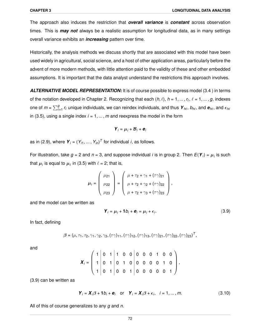
Figure 3.8 depicts for g = 2 groups and n = 3 time points two situations in which the mean responses

for each group for the three times lie on a straight line. In the left panel, the rate of change ,

represented by the slope of the two lines, is the same for both groups, so that the lines are parallel ,

whereas in the right panel the rate of change for group 2 is steeper than for group 1, so that the

lines are not parallel. Thus, in the left panel, the pattern of change is the same while in the right it is

different.

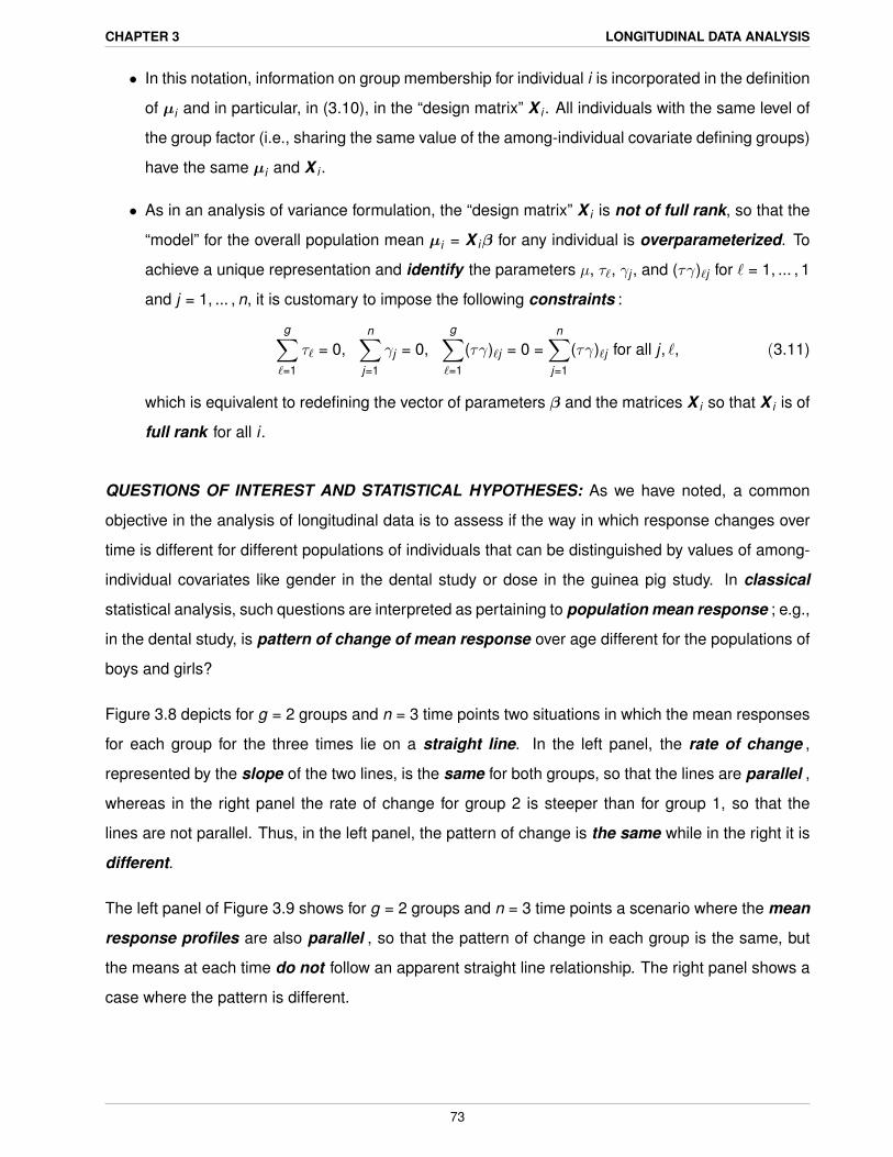
The left panel of Figure 3.9 shows for g = 2 groups and n = 3 time points a scenario where the mean

response profiles are also parallel , so that the pattern of change in each group is the same, but

the means at each time do not follow an apparent straight line relationship. The right panel shows a

case where the pattern is different.

73


Figure 3.8: Straight line mean profiles. Mean response for each group at each time, where the

plotting symbol indicates group number. There is no interaction in the left panel; the right panel

shows a quantitative interaction.

Figure 3.9: Mean profiles not a straight line.

74


GROUP BY TIME INTERACTION: In classical jargon, the situations in the right hand panels of

Figures 3.8 and 3.9 depict examples of a group by time interaction ; in each panel, the difference

in mean response between groups is not the same at all time points. In both figures, the direction

of the difference in mean response between groups is the same in that the mean for group 2 is

always larger. This is often referred to as a quantitative interaction , particularly in health sciences

research.

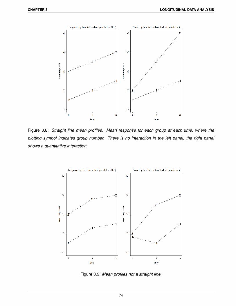
Figure 3.10: Crossed mean profiles. Each panel represents a form of qualitative interaction.

Figure 3.10 shows a different type of group by time interaction. In both panels, the difference in mean

response between groups is again not the same at all time points, and the direction of the difference

is not the same , either. For example, in the left hand panel, the magnitude of the difference at

times 1 and 3 is the same, but in the opposite direction. This is often referred to as a qualitative

interaction.

Returning to the model expressed using the classical notation as in (3.1), each mean in all of these

figures is represented by

µ`j = µ + τ` + γj + (τγ)`j .

The difference between mean response in groups 1 and 2 at any time j is, under this model,

µ1j − µ2j = (τ1 − τ2) + {(τγ)1j − (τγ)2j}.

75


Thus, the (τγ)`j allow the difference in means between groups to be different at different times j , as

in the right panels of Figures 3.8 and 3.9 and in Figure 3.10, by the amount {(τγ)1j − (τγ)2j )} at time

j .

If the (τγ)`j were all the same, the difference in means at any j reduces to

µ1j − µ2j = (τ1 − τ2),

so that the difference in mean response between groups is the same at all time points and equal

to (τ1 − τ2), which does not depend on j . This is the case in the left panels of Figures 3.8 and 3.9.

Here, the pattern of change over time is thus the same ; i.e., the mean profiles for each group are

parallel over time.

Under the constraintsg∑`=1

(τγ)`j = 0 =n∑

j=1

(τγ)`j for all `, j

in (3.11), if (τγ)`j are all the same for all `, j , then it must be that

(τγ)`j = 0 for all `, j .

In general, then, if we wish to address the question of whether or not there is a common pattern of

change over time, so whether or not the mean profiles are parallel, we can cast this in terms of the

null hypothesis

H0 : all (τγ)`j = 0, ` = 1, ... , g, j = 1, ... , n, (3.12)

with the alternative being that at least one (τγ)`j 6= 0, in which case the mean difference at at least

one of the time points is different from that at the others.

There are gn parameters (τγ)`j ; however, if the constraints above hold, then having (g − 1)(n − 1) of

the (τγ)`j equal to 0 automatically requires the remaining ones to be zero. Thus, the hypothesis (3.12)

is really one about the behavior of (g − 1)(n − 1) parameters, so there are (g − 1)(n − 1) degrees of

freedom associated with this hypothesis.

In the classical literature on analysis of variance for repeated measurements, the test of the null

hypothesis (3.12) is referred to as the test for parallelism. As Figure 3.9 demonstrates, parallelism

does not necessarily mean that the pattern of mean response in each group follow a straight line.

76


MAIN EFFECT OF GROUPS: If mean profiles are parallel, then the obvious next question is whether

or not they are coincident ; that is, whether or not the mean response is in fact the same for each

group at each time point. A little thought reveals that, if the mean profiles are parallel , if they are

furthermore coincident, then the average of the mean responses over time will be the same for each

group. The question of whether or not the average of mean responses is the same for each group if

the profiles are not parallel may or may not be interesting or relevant.

• If in truth the situation were like those depicted in the right hand panels of Figures 3.8 and 3.9,

whether or not the average of mean responses over time is different for the two groups might

be interesting, as it would reflect that the mean response for group 2 is larger at all times.

• On the other hand, consider the left panel of Figure 3.10. If this were the true state of affairs,

this issue is meaningless; the change of mean response over time is in the opposite direction

for the two groups; thus, how it averages out over time is of little importance. Because the

phenomenon of interest does indeed happen over time, the average of what it does over time

may be something that cannot be achieved – we can’t make time stand still.

• Similarly, if the issue under study is something like growth, the average over time of the re-

sponse may have little meaning; instead, one may be interested in, for example, how different

the mean response is at the end of the time period of study. For example, in the right panel of

Figure 3.10, mean response over time increases for each group at different rates, but has the

same average over time. The group with the steeper rate will have a larger mean response at

the end of the time period.

In general, then, the question of whether or not the average of the mean response over time is the

same across groups in a longitudinal study is of most interest when the mean profiles over time are

approximately parallel.

For definiteness, consider the case of g = 2 groups and n = 3 time points. For group `, the average

of means over time is, with n = 3,

n−1(µ`1 + µ`2 + µ`3) = µ + τ` + n−1(γ1 + γ2 + γ3) + n−1{(τγ)`1 + (τγ)`2 + (τγ)`3}.

The difference of the averages between ` = 1 and ` = 2 is then (algebra)

τ1 − τ2 + n−1n∑

j=1

(τγ)1j − n−1n∑

j=1

(τγ)2j .

77


The constraints (3.11) imposed to render the model of full rank dictate that∑n

j=1(τγ)`j = 0 for each

`; thus, the two sums in this expression are 0 by assumption, so that we are left with τ1 − τ2.

Thus, the hypothesis may be expressed as

H0 : τ1 − τ2 = 0.

Furthermore, under the constraint∑g

`=1 τ` = 0, if the τ` are equal as in H0, then they must satisfy

τ` = 0 for each `. Thus, the hypothesis may be rewritten as

H0 : τ1 = τ2 = 0.

For general g and n, the reasoning is the same; we have

H0 : τ1 = ... = τg = 0. (3.13)

MAIN EFFECT OF TIME: A further question of interest may be whether or not the mean response

is in fact constant over time. If the profiles are parallel, then this is like asking whether the mean

response averaged across groups is the same at each time. If the profiles are not parallel, then this

may or may not be interesting. For example, in the left panel of Figure 3.10, the average of mean

responses for groups 1 and 2 are the same at each time point. However, the mean response is

certainly not constant across time for either group. If the groups represent a factor like gender, then

what happens on average is something that can never be achieved.

The average of mean responses across groups for time j is

g−1g∑`=1

µ`j = γj + q−1g∑`=1

τ` + q−1g∑`=1

(τγ)`j = γj

using the constraints∑g

`=1 τ` = 0 and∑g

`=1(τγ)`j = 0 in (3.11). Thus, in the special case g = 2 and

n = 3, having all these averages be the same at each time is equivalent to

H0 : γ1 = γ2 = γ3.

Under the constraint∑n

j=1 γj = 0, then, we have H0 : γ1 = γ2 = γ3 = 0. For general g and n, the

hypothesis is of the form

H0 : γ1 = ... = γn = 0. (3.14)

78


REMARK: Hypotheses (3.12), (3.13), and (3.14) are, of course, exactly the hypotheses that one tests

for a split plot experiment , where, here, “time” plays the role of the “split plot” factor and “group” is

the “whole plot factor.” What is different is the interpretation ; because “time” has a natural ordering

(longitudinal), what is interesting may be different; as noted above, of primary interest is whether or

not the pattern of change in mean response over levels of time is different across groups.

ANALYSIS OF VARIANCE: Given that the statistical model and hypotheses of interest here are

identical to those for a split plot, it should come as no surprise that the analysis is identical. Under the

assumption that the model (3.1) is correctly specified and that the responses are normally distributed,

so that

Y h` ∼ Nn(µ`, V ), V = σ2bJn + σ2

eIn. (3.15)

as in (3.6), it can be shown the F ratios one would construct under the usual principles of analysis

of variance provide the basis for valid tests of the hypotheses above. For brevity, we present the

analysis of variance table and associated testing procedures without proof.

Define

• Y h`· = n−1∑nj=1 Yh`j , the sample average over time for the hth unit in the `th group (over all

observations on this unit)

• Y ·`j = r−1`

∑r`h=1 Yh`j , the sample average at time j in group ` over all units

• Y ·`· = (r`n)−1∑r`h=1∑n

j=1 Yh`j , the sample average of all observations in group `

• Y ··j = m−1∑g`=1∑r`

h=1 Yh`j , the sample average of all observations at the j th time

• Y ··· = the average of all mn observations.

Let

SSG =g∑`=1

nr`(Y ·`· − Y ···)2, SSTot ,U = ng∑`=1

r∑̀h=1

(Y h`· − Y ···)2

SST = mn∑

j=1

(Y ··j − Y ···)2, SSGT =n∑

j=1

g∑`=1

r`(Y ·`j − Y ···)2 − SST − SSG

SSTot ,all =g∑`=1

r∑̀h=1

n∑j=1

(Yh`j − Y ···)2.

Then the following analysis of variance table is constructed.

79


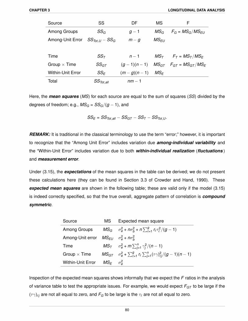
Source SS DF MS F

Among Groups SSG g − 1 MSG FG = MSG/MSEU

Among-Unit Error SSTot ,U − SSG m − g MSEU

Time SST n − 1 MST FT = MST/MSE

Group × Time SSGT (g − 1)(n − 1) MSGT FGT = MSGT/MSE

Within-Unit Error SSE (m − g)(n − 1) MSE

Total SSTot ,all nm − 1

Here, the mean squares (MS) for each source are equal to the sum of squares (SS) divided by the

degrees of freedom; e.g., MSG = SSG/(g − 1), and

SSE = SSTot ,all − SSGT − SST − SSTot ,U .

REMARK: It is traditional in the classical terminology to use the term “error;” however, it is important

to recognize that the “Among Unit Error” includes variation due among-individual variability and

the “Within-Unit Error” includes variation due to both within-individual realization (fluctuations )

and measurement error.

Under (3.15), the expectations of the mean squares in the table can be derived; we do not present

these calculations here (they can be found in Section 3.3 of Crowder and Hand, 1990). These

expected mean squares are shown in the following table; these are valid only if the model (3.15)

is indeed correctly specified, so that the true overall, aggregate pattern of correlation is compound

symmetric.

Source MS Expected mean square

Among Groups MSG σ2e + nσ2

b + n∑g

`=1 r`τ2` /(g − 1)

Among-Unit error MSEU σ2e + nσ2

b

Time MST σ2e + m

∑nj=1 γ

2j /(n − 1)

Group × Time MSGT σ2e +∑g

`=1 r`∑n

j=1(τγ)2`j/(g − 1)(n − 1)

Within-Unit Error MSE σ2e

Inspection of the expected mean squares shows informally that we expect the F ratios in the analysis

of variance table to test the appropriate issues. For example, we would expect FGT to be large if the

(τγ)`j are not all equal to zero, and FG to be large is the τ` are not all equal to zero.

80


Note that FG uses the appropriate denominator; intuitively, we wish to compare the mean square

for groups against an “error term” that takes into account all sources of variation among (σ2b) and

within (σ2e) individuals. The other two tests are on features that occur within individuals; thus, the

denominator takes account of the relevant source of variation, that within individuals (σ2e).

It can be shown formally that, as long as (3.15) is correctly specified, under the null hypotheses (3.12),

(3.13), and (3.14), the sampling distributions of the F ratios in the analysis of variance table are F

distributions with the degrees of freedom specified below.

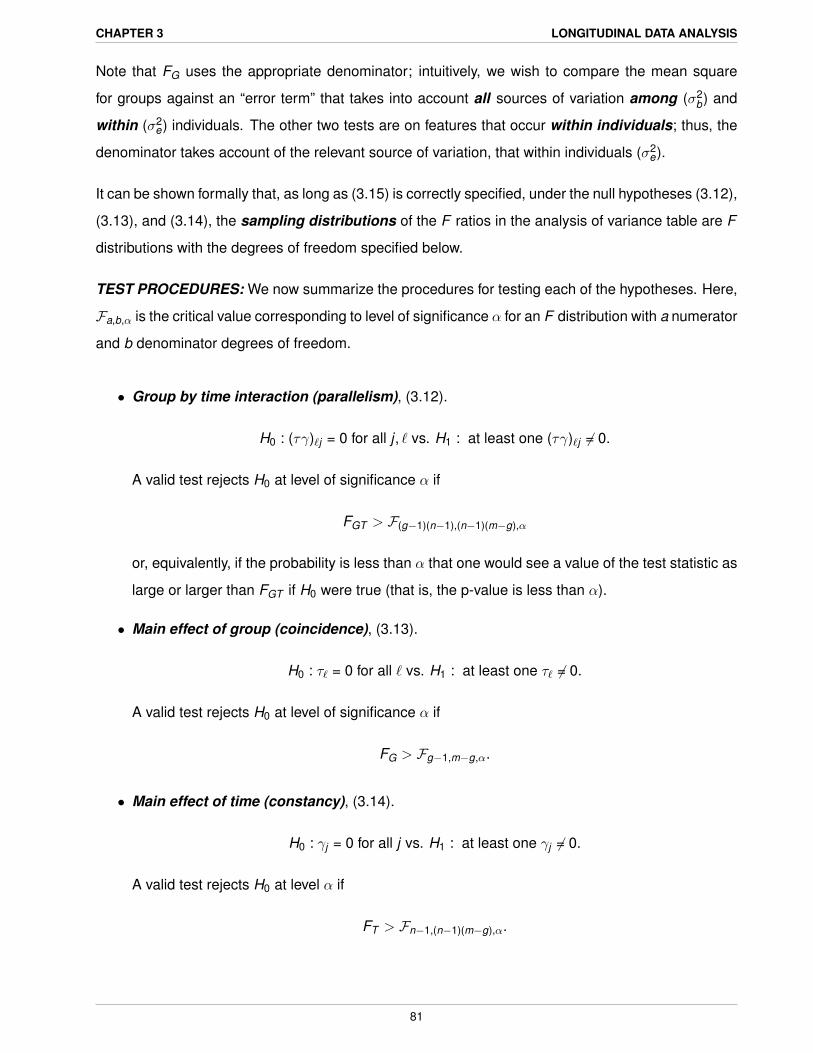
TEST PROCEDURES: We now summarize the procedures for testing each of the hypotheses. Here,

Fa,b,α is the critical value corresponding to level of significance α for an F distribution with a numerator

and b denominator degrees of freedom.

• Group by time interaction (parallelism), (3.12).

H0 : (τγ)`j = 0 for all j , ` vs. H1 : at least one (τγ)`j 6= 0.

A valid test rejects H0 at level of significance α if

FGT > F(g−1)(n−1),(n−1)(m−g),α

or, equivalently, if the probability is less than α that one would see a value of the test statistic as

large or larger than FGT if H0 were true (that is, the p-value is less than α).

• Main effect of group (coincidence), (3.13).

H0 : τ` = 0 for all ` vs. H1 : at least one τ` 6= 0.

A valid test rejects H0 at level of significance α if

FG > Fg−1,m−g,α.

• Main effect of time (constancy), (3.14).

H0 : γj = 0 for all j vs. H1 : at least one γj 6= 0.

A valid test rejects H0 at level α if

FT > Fn−1,(n−1)(m−g),α.

81


VIOLATION OF COVARIANCE MATRIX ASSUMPTION: These test procedures are valid under

model (3.15), which embodies the assumption of compound symmetry of the overall correlation

matrix of a data vector. In fact, it can be shown that they are also valid under slightly more general

conditions that include compound symmetry as a special case. However, validity of the tests is

predicated on the covariance matrix being of the special form we discuss next; if not, then F ratios

FT and FGT no longer have exactly an F distribution, and the associated tests are not valid and can

lead to erroneous conclusions.

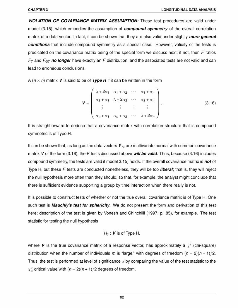
A (n × n) matrix V is said to be of Type H if it can be written in the form

V =

λ + 2α1 α1 + α2 · · · α1 + αn

α2 + α1 λ + 2α2 · · · α2 + αn...

......

...

αn + α1 αn + α2 · · · λ + 2αn

. (3.16)

It is straightforward to deduce that a covariance matrix with correlation structure that is compound

symmetric is of Type H.

It can be shown that, as long as the data vectors Y h` are multivariate normal with common covariance

matrix V of the form (3.16), the F tests discussed above will be valid. Thus, because (3.16) includes

compound symmetry, the tests are valid if model 3.15) holds. If the overall covariance matrix is not of

Type H, but these F tests are conducted nonetheless, they will be too liberal ; that is, they will reject

the null hypothesis more often than they should, so that, for example, the analyst might conclude that

there is sufficient evidence supporting a group by time interaction when there really is not.

It is possible to construct tests of whether or not the true overall covariance matrix is of Type H. One

such test is Mauchly’s test for sphericity. We do not present the form and derivation of this test

here; description of the test is given by Vonesh and Chinchilli (1997, p. 85), for example. The test

statistic for testing the null hypothesis

H0 : V is of Type H,

where V is the true covariance matrix of a response vector, has approximately a χ2 (chi-square)

distribution when the number of individuals m is “large,” with degrees of freedom (n − 2)(n + 1)/2.

Thus, the test is performed at level of significance α by comparing the value of the test statistic to the

χ2α critical value with (n − 2)(n + 1)/2 degrees of freedom.

82


All such tests have limitations : they are not very powerful with the numbers of individuals r` in each

group is not large, and they can be misleading if the true distribution of the response vectors is not

multivariate normal. Accordingly, we do not discuss it further. We return to the issue of approaches

when the analyst lacks confidence in the validity of the assumption of Type H covariance strutcure in

the next section.

3.3 Specialized within-individual hypotheses and tests

The hypotheses of group by time interaction (parallelism) and main effect of time (constancy) have

to do with questions about the pattern of change over time. However, they address these issues

in an “overall” sense; e.g., the test of the group by time interaction asks only if the pattern of mean

responses over time is different for different groups, but it does not provide insight into the nature

of the pattern of change and how it differs.

We now review methods to carry out a more detailed study of specific aspects of how the mean re-

sponse changes over time. As we demonstrate, these methods do this through testing of specialized

hypotheses.

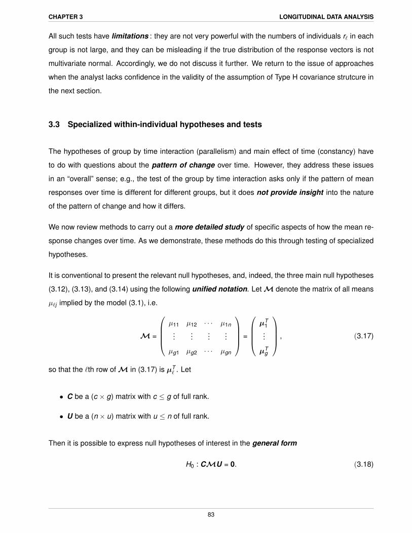
It is conventional to present the relevant null hypotheses, and, indeed, the three main null hypotheses

(3.12), (3.13), and (3.14) using the following unified notation. Let M denote the matrix of all means

µ`j implied by the model (3.1), i.e.

M =

µ11 µ12 · · · µ1n

......

......

µg1 µg2 · · · µgn

=

µT

1...

µTg

, (3.17)

so that the `th row of M in (3.17) is µT` . Let

• C be a (c × g) matrix with c ≤ g of full rank.

• U be a (n × u) matrix with u ≤ n of full rank.

Then it is possible to express null hypotheses of interest in the general form

H0 : CMU = 0. (3.18)

83


In this formulation

• the matrix C specifies differences among or averages across groups

• the matrix U specifies differences over or averages across levels of time.

Depending on the choices of the matrices C and U in (3.18), the resulting linear function CMU of

the elements of M (the individual means for different groups at different time points) can be made

to address specialized questions regarding differences in mean response among groups and in

patterns of change over time.

To see this, first consider the null hypothesis for the group by time interaction (parallelism) (3.12),

Ho : all (τγ)`j = 0, with g = 2 groups and n = 3 time points. Take

C =(

1, −1)

, (3.19)

so that c = 1 = g − 1. Note that

CM =(

1, −1) µ11 µ12 µ13

µ21 µ22 µ23

=(µ11 − µ21, µ12 − µ22, µ13 − µ23

)=(τ1 − τ2 + (τγ)11 − (τγ)21, τ1 − τ2 + (τγ)12 − (τγ)22, τ1 − τ2 + (τγ)13 − (τγ)23

)Thus, C yields differences in means among groups at each time point.

Take

U =

1 0

−1 1

0 −1

, (3.20)

so that u = 2 = n − 1. Thus, U involves differences for pairs of time points.

It is straightforward (try it) to show that

CMU =(µ11 − µ21 − µ12 + µ22, µ12 − µ22 − µ13 + µ23

)=(

(τγ)11 − (τγ)21 − (τγ)12 + (τγ)22, (τγ)12 − (τγ)22 − (τγ)13 + (τγ)23

).

It is an exercise in algebra to verify that, under the constraints in (3.11), if each of these elements

equals zero, then H0 follows.

84


Similarly, for the null hypothesis for the main effect of groups (coincidence), H0 : τ1 = τ2 = 0, taking

C to be as in (3.19) and

U =

1/3

1/3

1/3

,

it is straightforward to see that, with n = 3,

CMU = τ1 − τ2 + n−1n∑

j=1

(τγ)1j − n−1n∑

j=1

(τγ)2j .

That is, this choice of U dictates an averaging operation across time. Imposing the constraints as

above, we can express H0 in the form H0 : CMU = 0.

To express the null hypothesis for the main effect of time (constancy), H0 : γ1 = γ2 = γ3 = 0, take

U =

1 0

−1 1

0 −1

, C =(

1/2, 1/2)

.

Here, C involves averaging across groups while U involves differences for pairs of time points as

above. Then

MU =

µ11 µ12 µ13

µ21 µ22 µ23

1 0

−1 1

0 −1

=

µ11 − µ12 µ12 − µ13

µ21 − µ22 µ22 − µ23

(3.21)

=

γ1 − γ2 + (τγ)11 − (τγ)12, γ2 − γ3 + (τγ)12 − (τγ)13

γ1 − γ2 + (τγ)21 − (τγ)22, γ2 − γ3 + (τγ)22 − (τγ)23

.

from whence it is straightforward to derive, imposing the constraints in (3.11), that

CMU =(γ1 − γ2, γ2 − γ3

).

Setting this equal to zero with the constraint∑n

j=1 γj = 0 yields H0.

Clearly, the principles involved in specifying the matrices C and U to yield the form of the null hy-

potheses corresponding to the group by time interaction, main effect of groups, and main effect of

time generalize to any g and n.

85


Other choices of C and U can be made to examine components making up these overall hypotheses

and to isolate specific features of the pattern of change. Recall the following definition.

CONTRAST: If if c is a (n×1) vector and µ is a (n×1) vector of means, then the linear combination

cTµ = µT c is a contrast if c is such that its elements sum to zero; i.e., cT 1 = 0.

Thus, for example, with g = 2 and n = 3, the columns of the matrix

U =

1 0

−1 1

0 −1

in (3.20) define contrasts of elements of µ1 and µ2, the mean vectors for groups 1 and 2, in that

MU =

µ11 − µ12 µ12 − µ13

µ21 − µ22 µ22 − µ23

. (3.22)

In (3.22), each entry is a contrast involving differences in mean response between pairs of times in

each group. Specialized questions of interest can be posed by considering these contrasts.

• The difference of the contrasts in the first column of (3.22) focuses on whether or not the way

in which the mean response differs from time 1 to time 2 is different in groups 1 and 2. This

feature is clearly a component of the overall group by time interaction, focusing in particular on

times 1 and 2. Likewise, the difference of the contrasts in the second columns of (3.22) focuses

on the same for times 2 and 3, and is also part of the group by time interaction.

Indeed, taken together, the differences of constrasts in both columns of (3.22) fully character-

ize the overall group by time interaction.

• Similarly, the average of the contrasts in the first column of (3.22) focuses on the difference in

mean response between times 1 and 2, averaged across groups. This is clearly a component

of the main effect of time. Similarly, the average of contrasts in the second column reflects the

same for times 2 and 3. Again, taken together, the averages of contrasts in both rows of (3.22)

fully characterize the overall main effect of time.

Thus, considering these contrasts and their differences among or averages across groups serves to

“pick apart ” how the overall group by time interaction effect and main effect of time occur and can

provide insight into specific features of the pattern of change over time.

86


PROFILE TRANSFORMATION: For general number of groups g and number of time points n, the

extension of (3.20) is the (n × n − 1) matrix

U =

1 0 · · · 0

−1 1 · · · 0

0 −1 · · · 0...

......

...

0 · · · · · · 1

0 · · · 0 −1

. (3.23)

Postmultiplication of M by U in (3.23) results in contrasts comparing means at successive pairs of

time points and is often called the profile transformation of the means. Examining individually the

differences among or averages across the contrasts resulting from each column provides insight on

the contribution to the overall pattern of change over time.

Other U matrices allow other ways of “parsing” the pattern of change over time. For example, instead

of focusing on changes from one time to the next, one might consider how the mean at a specific time

point differs from what happens at all subsequent time points. This might highlight at what point in

time changes in the pattern begin to emerge.

We demonstrate with g = 2 and n = 4 and consider the contrast

µ11 − (µ12 + µ13 + µ14)/3,

which compares, for group 1, the mean at time 1 to the average of means at all other times. Similarly,

µ12 − (µ13 + µ14)/2

compares for group 1 the mean at time 2 to the average of those at subsequent times. The final

contrast of this type for group 1 is

µ13 − µ14,

which compares what happens at time 3 to the “average” of what comes next, the single mean at

time 4. We may similarly specify such contrasts for the other group.

87


These contrasts can be obtained by postmultiplying M by

U =

1 0 0

−1/3 1 0

−1/3 −1/2 1

−1/3 −1/2 −1

. (3.24)

In particular, with g = 2,

MU =

µ11 − µ12/3− µ13/3− µ14/3, µ12 − µ13/2− µ14/2, µ13 − µ14

µ21 − µ22/3− µ23/3− µ24/3, µ22 − µ23/2− µ24/2, µ23 − µ24

. (3.25)

HELMERT TRANSFORMATION: For general n, the (n×n−1) matrix whose columns define contrasts

of this type is the so-called Helmert transformation matrix of the form

U =

1 0 0 · · · 0

−1/(n − 1) 1 0 · · · 0

−1/(n − 1) −1/(n − 2) 1 · · · 0...

... −1/(n − 3)...

...

−1/(n − 1) −1/(n − 2)... · · · 1

−1/(n − 1) −1/(n − 2) −1/(n − 3) · · · −1

. (3.26)

Postmultiplication of M by a matrix of the form (3.26) yields contrasts representing comparisons of

each mean against the average of means at all subsequent times.

It is in fact the case that any U matrix with n−1 columns, so involving n−1 constrasts that “pick apart”

all possible differences in means over time, as do the profile and Helmert transformation matrices

(3.23) and (3.26), lead to the overall hypotheses for group by time interaction and main effect of time

when paired with the appropriate C matrix.

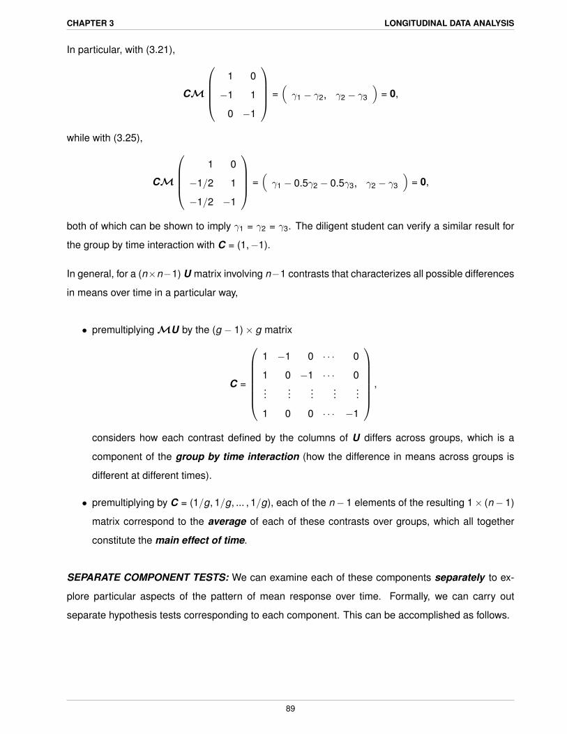
For example, in the case g = 2, n = 3, if we premultiply either of (3.21) or (3.25) by C = (1/2, 1/2)

and impose the constraints (3.11), we are led to the null hypothesis H0 : γ1 = γ2 = γ3 = 0 for the main

effect of time.

88


In particular, with (3.21),

CM

1 0

−1 1

0 −1

=(γ1 − γ2, γ2 − γ3

)= 0,

while with (3.25),

CM

1 0

−1/2 1

−1/2 −1

=(γ1 − 0.5γ2 − 0.5γ3, γ2 − γ3

)= 0,

both of which can be shown to imply γ1 = γ2 = γ3. The diligent student can verify a similar result for

the group by time interaction with C = (1,−1).

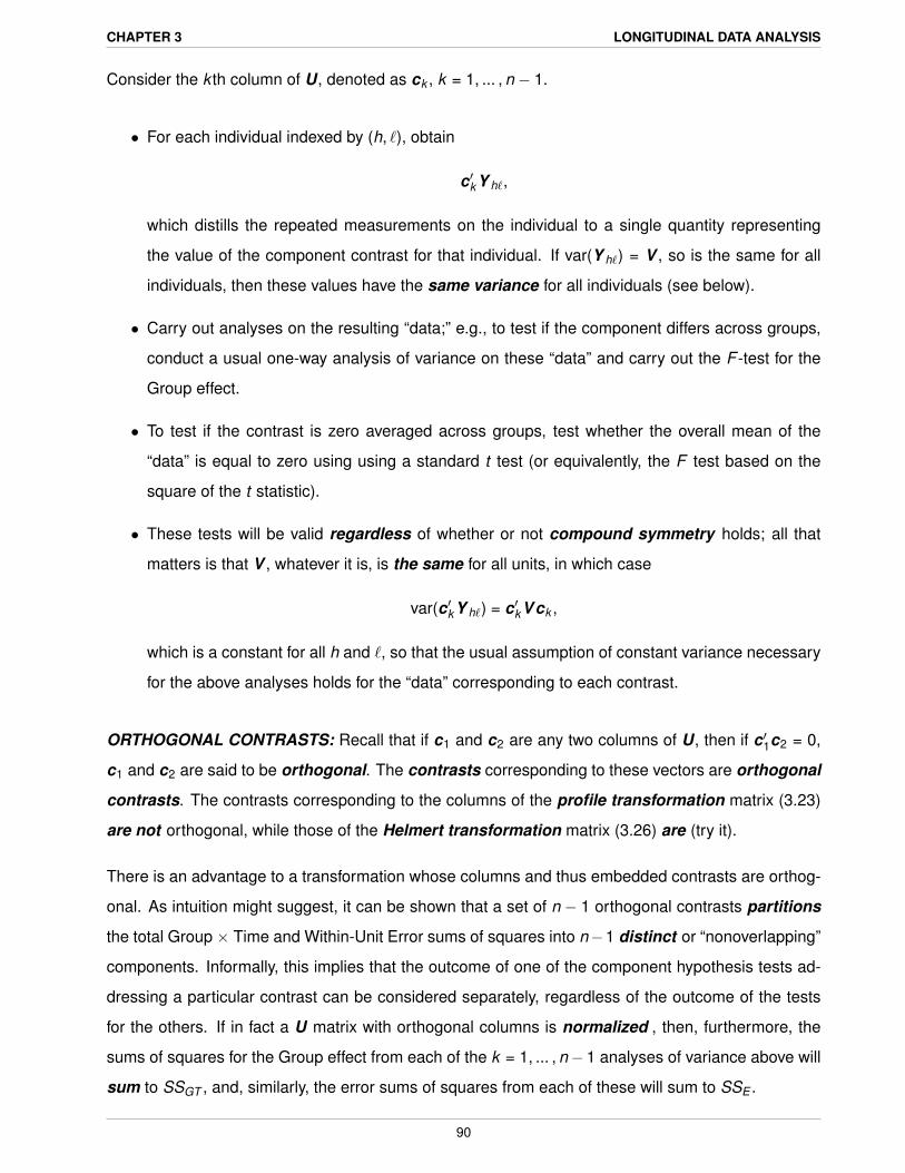
In general, for a (n×n−1) U matrix involving n−1 contrasts that characterizes all possible differences

in means over time in a particular way,

• premultiplying MU by the (g − 1)× g matrix

C =

1 −1 0 · · · 0

1 0 −1 · · · 0...

......

......

1 0 0 · · · −1

,

considers how each contrast defined by the columns of U differs across groups, which is a

component of the group by time interaction (how the difference in means across groups is

different at different times).

• premultiplying by C = (1/g, 1/g, ... , 1/g), each of the n− 1 elements of the resulting 1× (n− 1)

matrix correspond to the average of each of these contrasts over groups, which all together

constitute the main effect of time.

SEPARATE COMPONENT TESTS: We can examine each of these components separately to ex-

plore particular aspects of the pattern of mean response over time. Formally, we can carry out

separate hypothesis tests corresponding to each component. This can be accomplished as follows.

89


Consider the k th column of U, denoted as ck , k = 1, ... , n − 1.

• For each individual indexed by (h, `), obtain

c′kY h`,

which distills the repeated measurements on the individual to a single quantity representing

the value of the component contrast for that individual. If var(Y h`) = V , so is the same for all

individuals, then these values have the same variance for all individuals (see below).

• Carry out analyses on the resulting “data;” e.g., to test if the component differs across groups,

conduct a usual one-way analysis of variance on these “data” and carry out the F -test for the

Group effect.

• To test if the contrast is zero averaged across groups, test whether the overall mean of the

“data” is equal to zero using using a standard t test (or equivalently, the F test based on the

square of the t statistic).

• These tests will be valid regardless of whether or not compound symmetry holds; all that

matters is that V , whatever it is, is the same for all units, in which case

var(c′kY h`) = c′kVck ,

which is a constant for all h and `, so that the usual assumption of constant variance necessary

for the above analyses holds for the “data” corresponding to each contrast.

ORTHOGONAL CONTRASTS: Recall that if c1 and c2 are any two columns of U, then if c′1c2 = 0,

c1 and c2 are said to be orthogonal. The contrasts corresponding to these vectors are orthogonal

contrasts. The contrasts corresponding to the columns of the profile transformation matrix (3.23)

are not orthogonal, while those of the Helmert transformation matrix (3.26) are (try it).

There is an advantage to a transformation whose columns and thus embedded contrasts are orthog-

onal. As intuition might suggest, it can be shown that a set of n − 1 orthogonal contrasts partitions

the total Group × Time and Within-Unit Error sums of squares into n−1 distinct or “nonoverlapping”

components. Informally, this implies that the outcome of one of the component hypothesis tests ad-

dressing a particular contrast can be considered separately, regardless of the outcome of the tests

for the others. If in fact a U matrix with orthogonal columns is normalized , then, furthermore, the

sums of squares for the Group effect from each of the k = 1, ... , n− 1 analyses of variance above will

sum to SSGT , and, similarly, the error sums of squares from each of these will sum to SSE .

90


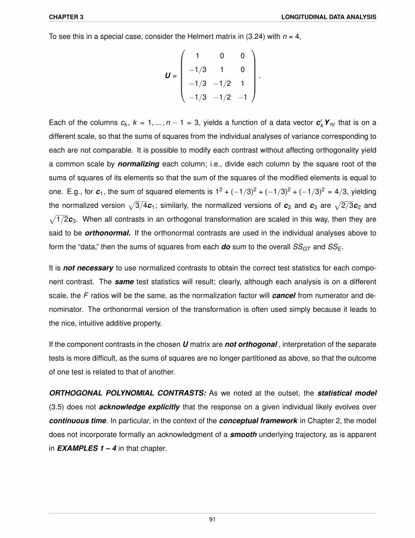
To see this in a special case, consider the Helmert matrix in (3.24) with n = 4,

U =

1 0 0

−1/3 1 0

−1/3 −1/2 1

−1/3 −1/2 −1

.

Each of the columns ck , k = 1, ... , n − 1 = 3, yields a function of a data vector c′kY h` that is on a

different scale, so that the sums of squares from the individual analyses of variance corresponding to

each are not comparable. It is possible to modify each contrast without affecting orthogonality yield

a common scale by normalizing each column; i.e., divide each column by the square root of the

sums of squares of its elements so that the sum of the squares of the modified elements is equal to

one. E.g., for c1, the sum of squared elements is 12 + (−1/3)2 + (−1/3)2 + (−1/3)2 = 4/3, yielding

the normalized version√

3/4c1; similarly, the normalized versions of c2 and c3 are√

2/3c2 and√1/2c3. When all contrasts in an orthogonal transformation are scaled in this way, then they are

said to be orthonormal. If the orthonormal contrasts are used in the individual analyses above to

form the “data,” then the sums of squares from each do sum to the overall SSGT and SSE .

It is not necessary to use normalized contrasts to obtain the correct test statistics for each compo-

nent contrast. The same test statistics will result; clearly, although each analysis is on a different

scale, the F ratios will be the same, as the normalization factor will cancel from numerator and de-

nominator. The orthonormal version of the transformation is often used simply because it leads to

the nice, intuitive additive property.

If the component contrasts in the chosen U matrix are not orthogonal , interpretation of the separate

tests is more difficult, as the sums of squares are no longer partitioned as above, so that the outcome

of one test is related to that of another.

ORTHOGONAL POLYNOMIAL CONTRASTS: As we noted at the outset, the statistical model

(3.5) does not acknowledge explicitly that the response on a given individual likely evolves over

continuous time. In particular, in the context of the conceptual framework in Chapter 2, the model

does not incorporate formally an acknowledgment of a smooth underlying trajectory, as is apparent

in EXAMPLES 1 – 4 in that chapter.

91


Accordingly, there is a need to be able to evaluate behavior of the mean response over (continuous)

time in the context of the statistical model that acknowledges possible smooth patterns of change.

For example, in the dental study, we might wish to evaluate whether or not there is a linear or in fact

quadratic trend over time, averaged across genders and whether or not the linear or quadratic trend

differs between genders.

This is facilitated by, for n time points, the set of n − 1 orthogonal polynomial contrasts. These

contrasts are based on the premise that, with data at the same n time points, it is possible to fit up to a

(n−1)th degree polynomial in time. Thus, just as the profile and Helmert transformations decompose

the overall time effect into n − 1 contrasts addressing specific differences over time, these contrasts

decompose this into orthogonal components reflecting the strength of linear, quadratic, cubic, and

so on contributions to the saturated (n − 1)th degree polynomial. This is possible for times that are

equally or unequally spaced; we do not present derivations here. For equally-spaced time points,

the coefficients of the n− 1 orthogonal polynomials are available in many classical statistics texts; for

unequally-spaced times, the coefficients depend on the times themselves.

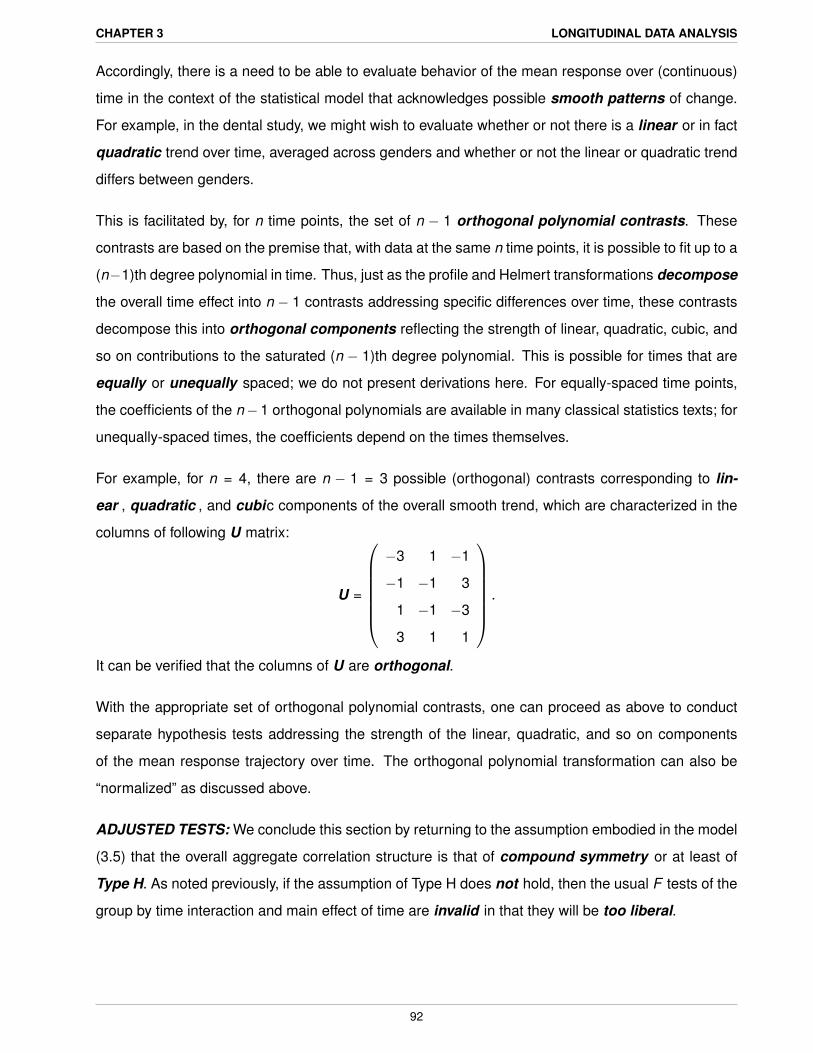
For example, for n = 4, there are n − 1 = 3 possible (orthogonal) contrasts corresponding to lin-

ear , quadratic , and cubic components of the overall smooth trend, which are characterized in the

columns of following U matrix:

U =

−3 1 −1

−1 −1 3

1 −1 −3

3 1 1

.

It can be verified that the columns of U are orthogonal.

With the appropriate set of orthogonal polynomial contrasts, one can proceed as above to conduct

separate hypothesis tests addressing the strength of the linear, quadratic, and so on components

of the mean response trajectory over time. The orthogonal polynomial transformation can also be

“normalized” as discussed above.

ADJUSTED TESTS: We conclude this section by returning to the assumption embodied in the model

(3.5) that the overall aggregate correlation structure is that of compound symmetry or at least of

Type H. As noted previously, if the assumption of Type H does not hold, then the usual F tests of the

group by time interaction and main effect of time are invalid in that they will be too liberal.

92


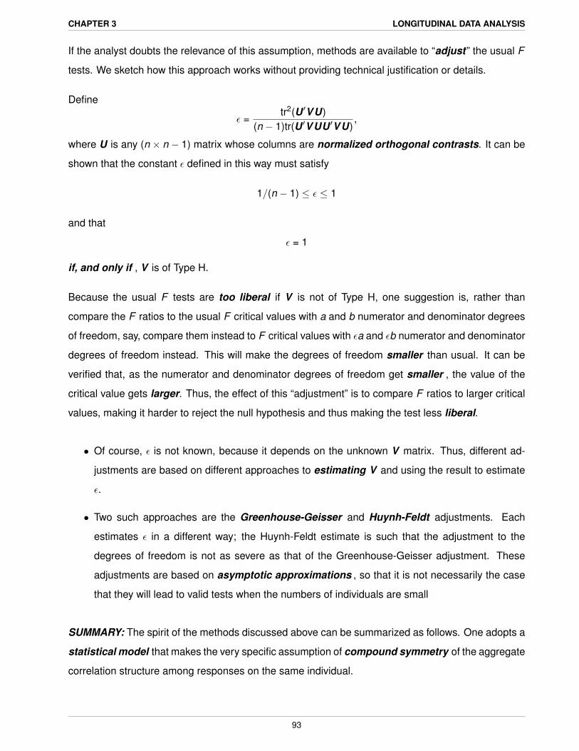
If the analyst doubts the relevance of this assumption, methods are available to “adjust” the usual F

tests. We sketch how this approach works without providing technical justification or details.

Define

ε =tr2(U ′VU)

(n − 1)tr(U ′VUU ′VU),

where U is any (n × n − 1) matrix whose columns are normalized orthogonal contrasts. It can be

shown that the constant ε defined in this way must satisfy

1/(n − 1) ≤ ε ≤ 1

and that

ε = 1

if, and only if , V is of Type H.

Because the usual F tests are too liberal if V is not of Type H, one suggestion is, rather than

compare the F ratios to the usual F critical values with a and b numerator and denominator degrees

of freedom, say, compare them instead to F critical values with εa and εb numerator and denominator

degrees of freedom instead. This will make the degrees of freedom smaller than usual. It can be

verified that, as the numerator and denominator degrees of freedom get smaller , the value of the

critical value gets larger. Thus, the effect of this “adjustment” is to compare F ratios to larger critical

values, making it harder to reject the null hypothesis and thus making the test less liberal.

• Of course, ε is not known, because it depends on the unknown V matrix. Thus, different ad-

justments are based on different approaches to estimating V and using the result to estimate

ε.

• Two such approaches are the Greenhouse-Geisser and Huynh-Feldt adjustments. Each

estimates ε in a different way; the Huynh-Feldt estimate is such that the adjustment to the

degrees of freedom is not as severe as that of the Greenhouse-Geisser adjustment. These

adjustments are based on asymptotic approximations , so that it is not necessarily the case

that they will lead to valid tests when the numbers of individuals are small

SUMMARY: The spirit of the methods discussed above can be summarized as follows. One adopts a

statistical model that makes the very specific assumption of compound symmetry of the aggregate

correlation structure among responses on the same individual.

93


If this assumption is correct, then familiar analysis of variance methods are available to test hy-

potheses regarding the pattern of change over time and mean response averaged across groups.

However, the model does not lend itself readily to estimation of features of the pattern of change,

and the procedures to construct tests to study different features of the pattern are rather unwieldy.

It is possible to carry out a test of whether or not the compound symmetry assumption is supported

by the data; however, the testing procedures are not reliable. Approximate, “adjusted” versions of the

tests are available, but these are not necessarily reliable, either.

The bottom line is that a better approach might be to start with a more realistic and flexible statistical

model within which to characterize and evaluate features of the pattern of change. This is the basis

for the more modern methods we study in later chapters.

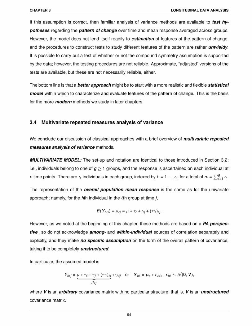
3.4 Multivariate repeated measures analysis of variance

We conclude our discussion of classical approaches with a brief overview of multivariate repeated

measures analysis of variance methods.

MULTIVARIATE MODEL: The set-up and notation are identical to those introduced in Section 3.2;

i.e., individuals belong to one of g ≥ 1 groups, and the response is ascertained on each individual at

n time points. There are r` individuals in each group, indexed by h = 1 ... , r`, for a total of m =∑g

`=1 r`.

The representation of the overall population mean response is the same as for the univariate

approach; namely, for the hth individual in the `th group at time j ,

E(Yh`j ) = µ`j = µ + τ` + γj + (τγ)`j .

However, as we noted at the beginning of this chapter, these methods are based on a PA perspec-

tive , so do not acknowledge among- and within-individual sources of correlation separately and

explicitly, and they make no specific assumption on the form of the overall pattern of covariance,

taking it to be completely unstructured.

In particular, the assumed model is

Yh`j = µ + τ` + γj + (τγ)`j︸︷︷︸µ`j

+εh`j or Y h` = µ` + εh`, εh` ∼ N (0, V ),

where V is an arbitrary covariance matrix with no particular structure; that is, V is an unstructured

covariance matrix.

94


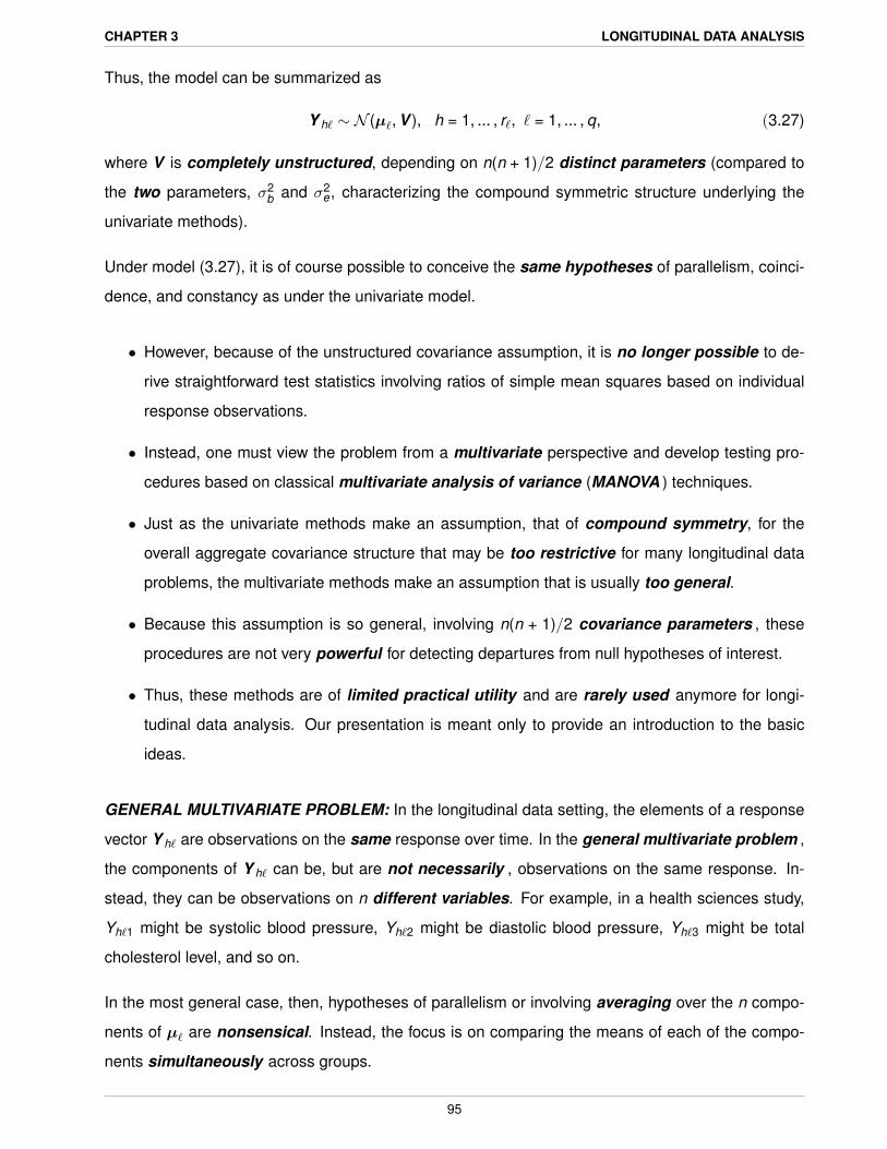
Thus, the model can be summarized as

Y h` ∼ N (µ`, V ), h = 1, ... , r`, ` = 1, ... , q, (3.27)

where V is completely unstructured, depending on n(n + 1)/2 distinct parameters (compared to

the two parameters, σ2b and σ2

e, characterizing the compound symmetric structure underlying the

univariate methods).

Under model (3.27), it is of course possible to conceive the same hypotheses of parallelism, coinci-

dence, and constancy as under the univariate model.

• However, because of the unstructured covariance assumption, it is no longer possible to de-

rive straightforward test statistics involving ratios of simple mean squares based on individual

response observations.

• Instead, one must view the problem from a multivariate perspective and develop testing pro-

cedures based on classical multivariate analysis of variance (MANOVA ) techniques.

• Just as the univariate methods make an assumption, that of compound symmetry, for the

overall aggregate covariance structure that may be too restrictive for many longitudinal data

problems, the multivariate methods make an assumption that is usually too general.

• Because this assumption is so general, involving n(n + 1)/2 covariance parameters , these

procedures are not very powerful for detecting departures from null hypotheses of interest.

• Thus, these methods are of limited practical utility and are rarely used anymore for longi-

tudinal data analysis. Our presentation is meant only to provide an introduction to the basic

ideas.

GENERAL MULTIVARIATE PROBLEM: In the longitudinal data setting, the elements of a response

vector Y h` are observations on the same response over time. In the general multivariate problem ,

the components of Y h` can be, but are not necessarily , observations on the same response. In-

stead, they can be observations on n different variables. For example, in a health sciences study,

Yh`1 might be systolic blood pressure, Yh`2 might be diastolic blood pressure, Yh`3 might be total

cholesterol level, and so on.

In the most general case, then, hypotheses of parallelism or involving averaging over the n compo-

nents of µ` are nonsensical. Instead, the focus is on comparing the means of each of the compo-

nents simultaneously across groups.

95


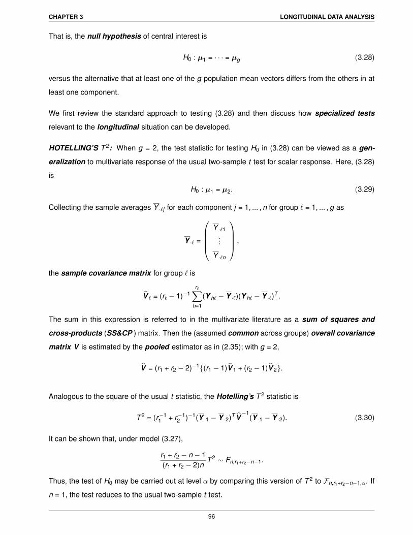
That is, the null hypothesis of central interest is

H0 : µ1 = · · · = µg (3.28)

versus the alternative that at least one of the g population mean vectors differs from the others in at

least one component.

We first review the standard approach to testing (3.28) and then discuss how specialized tests

relevant to the longitudinal situation can be developed.

HOTELLING’S T 2: When g = 2, the test statistic for testing H0 in (3.28) can be viewed as a gen-

eralization to multivariate response of the usual two-sample t test for scalar response. Here, (3.28)

is

H0 : µ1 = µ2. (3.29)

Collecting the sample averages Y ·`j for each component j = 1, ... , n for group ` = 1, ... , g as

Y ·` =

Y ·`1

...

Y ·`n

,

the sample covariance matrix for group ` is

V̂ ` = (r` − 1)−1r∑̀

h=1

(Y h` − Y ·`)(Y h` − Y ·`)T .

The sum in this expression is referred to in the multivariate literature as a sum of squares and

cross-products (SS&CP ) matrix. Then the (assumed common across groups) overall covariance

matrix V is estimated by the pooled estimator as in (2.35); with g = 2,

V̂ = (r1 + r2 − 2)−1{(r1 − 1)V̂ 1 + (r2 − 1)V̂ 2}.

Analogous to the square of the usual t statistic, the Hotelling’s T 2 statistic is

T 2 = (r−11 + r−1

2 )−1(Y ·1 − Y ·2)T V̂−1

(Y ·1 − Y ·2). (3.30)

It can be shown that, under model (3.27),

r1 + r2 − n − 1(r1 + r2 − 2)n

T 2 ∼ Fn,r1+r2−n−1.

Thus, the test of H0 may be carried out at level α by comparing this version of T 2 to Fn,r1+r2−n−1,α. If

n = 1, the test reduces to the usual two-sample t test.

96


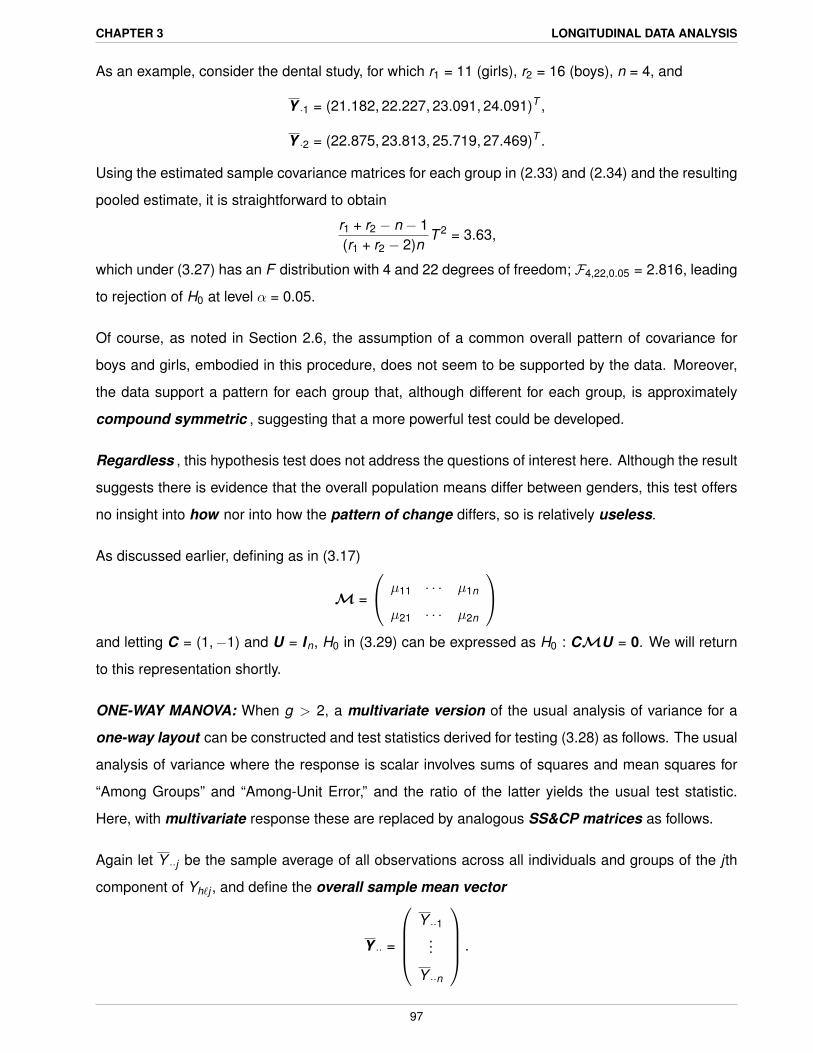
As an example, consider the dental study, for which r1 = 11 (girls), r2 = 16 (boys), n = 4, and

Y ·1 = (21.182, 22.227, 23.091, 24.091)T ,

Y ·2 = (22.875, 23.813, 25.719, 27.469)T .

Using the estimated sample covariance matrices for each group in (2.33) and (2.34) and the resulting

pooled estimate, it is straightforward to obtain

r1 + r2 − n − 1(r1 + r2 − 2)n

T 2 = 3.63,

which under (3.27) has an F distribution with 4 and 22 degrees of freedom; F4,22,0.05 = 2.816, leading

to rejection of H0 at level α = 0.05.

Of course, as noted in Section 2.6, the assumption of a common overall pattern of covariance for

boys and girls, embodied in this procedure, does not seem to be supported by the data. Moreover,

the data support a pattern for each group that, although different for each group, is approximately

compound symmetric , suggesting that a more powerful test could be developed.

Regardless , this hypothesis test does not address the questions of interest here. Although the result

suggests there is evidence that the overall population means differ between genders, this test offers

no insight into how nor into how the pattern of change differs, so is relatively useless.

As discussed earlier, defining as in (3.17)

M =

µ11 · · · µ1n

µ21 · · · µ2n

and letting C = (1,−1) and U = In, H0 in (3.29) can be expressed as H0 : CMU = 0. We will return

to this representation shortly.

ONE-WAY MANOVA: When g > 2, a multivariate version of the usual analysis of variance for a

one-way layout can be constructed and test statistics derived for testing (3.28) as follows. The usual

analysis of variance where the response is scalar involves sums of squares and mean squares for

“Among Groups” and “Among-Unit Error,” and the ratio of the latter yields the usual test statistic.

Here, with multivariate response these are replaced by analogous SS&CP matrices as follows.

Again let Y ··j be the sample average of all observations across all individuals and groups of the j th

component of Yh`j , and define the overall sample mean vector

Y ·· =

Y ··1

...

Y ··n

.

97


Then construct the MANOVA table as

Source SS&CP DF

Among Groups QH =∑g

`=1 r`(Y ·` − Y ··)(Y ·` − Y ··)T g − 1

Among-unit Error QE =∑g

`=1∑r`

h=1(Y h` − Y ·`)(Y h` − Y ·`)T m − g

Total QH + QE =∑g

`=1∑r`

h=1(Y h` − Y ··)(Y h` − Y ··)T m − 1

It can be verified that

QE = (r1 − 1)V̂ 1 + · · · + (rg − 1)V̂ g ,

so that

V̂ = QE/(m − g).

Because the entries in the MANOVA table are matrices , it is not straightforward to construct a unique

generalization of the usual analysis of variance F ratio that can be used to test H0 in (3.28). Clearly,

one would like to compare the “magnitudes ” of the SS&CP matrices QH and QE , but there is no one

way to do this. Several statistics have been proposed.

• The most commonly discussed statistic is Wilks’ lambda , which can be motivated informally

as follows. Letting SSG and SSE be the usual analysis of variance Among-Groups and Among-

Unit Error sums of squares, the familiar F ratio is

SSG/(g − 1)SSE/(m − g)

.

Thus, in the scalar case, H0 is rejected when SSG/SSE is “large.” This is equivalent to rejecting

for large values of 1 + SSG/SSE or small values of

11 + SSG/SSE

=SSE

SSG + SSE.

For the multivariate problem, the Wilks’ lambda statistic is the analog of this quantity,

TW =|QE |

|QH + QE |.

One rejects H0 for “small” values of TW .

• The Lawley-Hotelling trace rejects H0 for large values of

TLH = tr(QHQ−1E ).

• Other statistics are Pillai’s trace and Roy’s greatest root, which we do not present.

• None of these approaches has been shown to be superior to the others in general. All are

equivalent to using the Hotelling T 2 statistic in the case g = 2.

98


A full discussion of these methods is beyond our scope. For general g and n, the sampling distribu-

tions of (functions of) these test statistics may or may not be derived exactly. Thus, except in certain

special cases where this is possible (see Johnson and Wichern, 2002), the sampling distributions are

approximated by the F or other distributions.

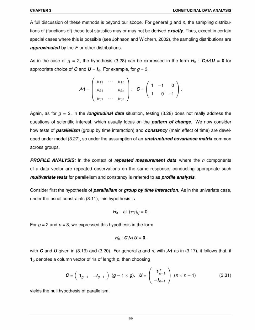
As in the case of g = 2, the hypothesis (3.28) can be expressed in the form H0 : CMU = 0 for

appropriate choice of C and U = In. For example, for g = 3,

M =

µ11 · · · µ1n

µ21 · · · µ2n

µ31 · · · µ3n

, C =

1 −1 0

1 0 −1

.

Again, as for g = 2, in the longitudinal data situation, testing (3.28) does not really address the

questions of scientific interest, which usually focus on the pattern of change. We now consider

how tests of parallelism (group by time interaction) and constancy (main effect of time) are devel-

oped under model (3.27), so under the assumption of an unstructured covariance matrix common

across groups.

PROFILE ANALYSIS: In the context of repeated measurement data where the n components

of a data vector are repeated observations on the same response, conducting appropriate such

multivariate tests for parallelism and constancy is referred to as profile analysis.

Consider first the hypothesis of parallelism or group by time interaction. As in the univariate case,

under the usual constraints (3.11), this hypothesis is

H0 : all (τγ)`j = 0.

For g = 2 and n = 3, we expressed this hypothesis in the form

H0 : CMU = 0,

with C and U given in (3.19) and (3.20). For general g and n, with M as in (3.17), it follows that, if

1p denotes a column vector of 1s of length p, then choosing

C =(

1g−1 −Ig−1

)(g − 1× g), U =

1Tn−1

−In−1

(n × n − 1) (3.31)

yields the null hypothesis of parallelism.

99


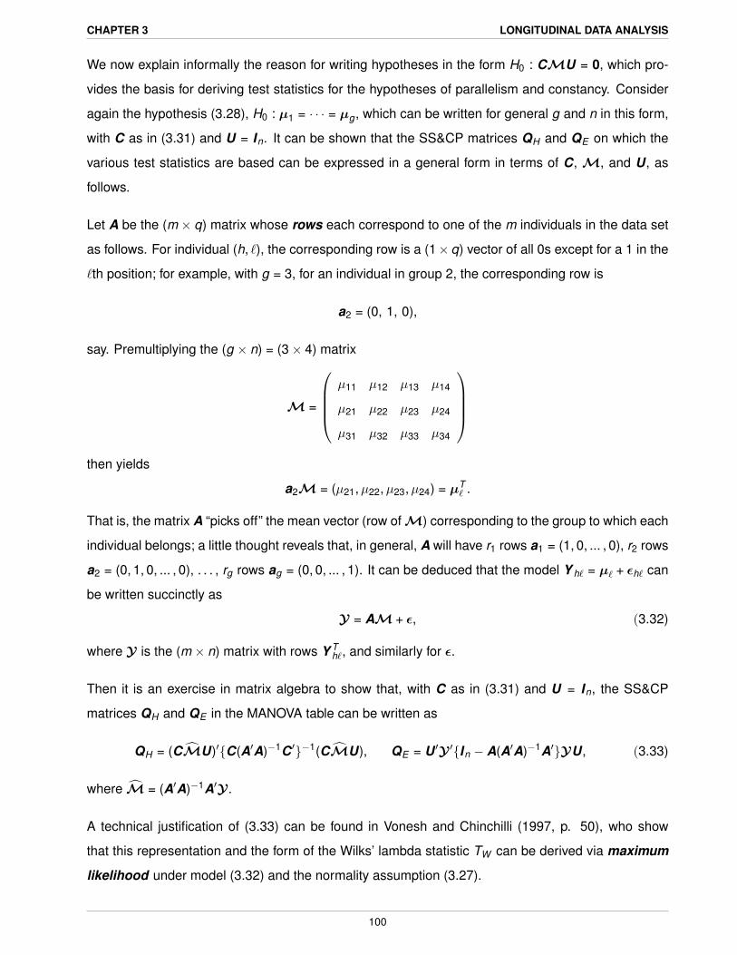
We now explain informally the reason for writing hypotheses in the form H0 : CMU = 0, which pro-

vides the basis for deriving test statistics for the hypotheses of parallelism and constancy. Consider

again the hypothesis (3.28), H0 : µ1 = · · · = µg , which can be written for general g and n in this form,

with C as in (3.31) and U = In. It can be shown that the SS&CP matrices QH and QE on which the

various test statistics are based can be expressed in a general form in terms of C, M, and U, as

follows.

Let A be the (m × q) matrix whose rows each correspond to one of the m individuals in the data set

as follows. For individual (h, `), the corresponding row is a (1× q) vector of all 0s except for a 1 in the

`th position; for example, with g = 3, for an individual in group 2, the corresponding row is

a2 = (0, 1, 0),

say. Premultiplying the (g × n) = (3× 4) matrix

M =

µ11 µ12 µ13 µ14

µ21 µ22 µ23 µ24

µ31 µ32 µ33 µ34

then yields

a2M = (µ21,µ22,µ23,µ24) = µT` .

That is, the matrix A “picks off” the mean vector (row of M) corresponding to the group to which each

individual belongs; a little thought reveals that, in general, A will have r1 rows a1 = (1, 0, ... , 0), r2 rows

a2 = (0, 1, 0, ... , 0), . . . , rg rows ag = (0, 0, ... , 1). It can be deduced that the model Y h` = µ` + εh` can

be written succinctly as

Y = AM + ε, (3.32)

where Y is the (m × n) matrix with rows Y Th`, and similarly for ε.

Then it is an exercise in matrix algebra to show that, with C as in (3.31) and U = In, the SS&CP

matrices QH and QE in the MANOVA table can be written as

QH = (CM̂U)′{C(A′A)−1C ′}−1(CM̂U), QE = U ′Y ′{In − A(A′A)−1A′}YU, (3.33)

where M̂ = (A′A)−1A′Y .

A technical justification of (3.33) can be found in Vonesh and Chinchilli (1997, p. 50), who show

that this representation and the form of the Wilks’ lambda statistic TW can be derived via maximum

likelihood under model (3.32) and the normality assumption (3.27).

100


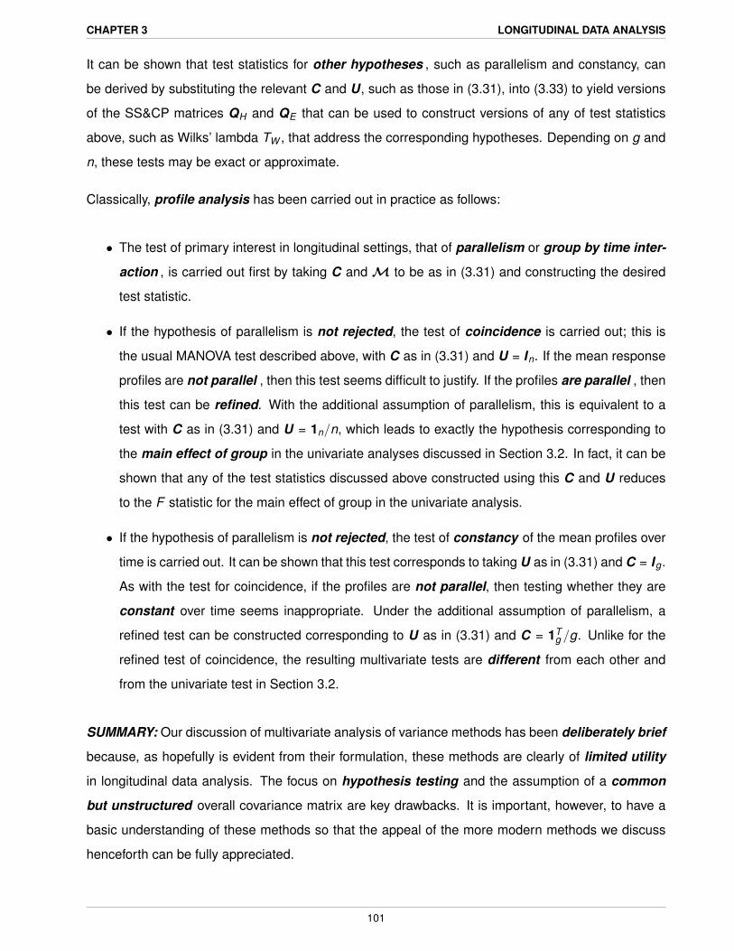
It can be shown that test statistics for other hypotheses , such as parallelism and constancy, can

be derived by substituting the relevant C and U, such as those in (3.31), into (3.33) to yield versions

of the SS&CP matrices QH and QE that can be used to construct versions of any of test statistics

above, such as Wilks’ lambda TW , that address the corresponding hypotheses. Depending on g and

n, these tests may be exact or approximate.

Classically, profile analysis has been carried out in practice as follows:

• The test of primary interest in longitudinal settings, that of parallelism or group by time inter-

action , is carried out first by taking C and M to be as in (3.31) and constructing the desired

test statistic.

• If the hypothesis of parallelism is not rejected, the test of coincidence is carried out; this is

the usual MANOVA test described above, with C as in (3.31) and U = In. If the mean response

profiles are not parallel , then this test seems difficult to justify. If the profiles are parallel , then

this test can be refined. With the additional assumption of parallelism, this is equivalent to a

test with C as in (3.31) and U = 1n/n, which leads to exactly the hypothesis corresponding to

the main effect of group in the univariate analyses discussed in Section 3.2. In fact, it can be

shown that any of the test statistics discussed above constructed using this C and U reduces

to the F statistic for the main effect of group in the univariate analysis.

• If the hypothesis of parallelism is not rejected, the test of constancy of the mean profiles over

time is carried out. It can be shown that this test corresponds to taking U as in (3.31) and C = Ig .

As with the test for coincidence, if the profiles are not parallel, then testing whether they are

constant over time seems inappropriate. Under the additional assumption of parallelism, a

refined test can be constructed corresponding to U as in (3.31) and C = 1Tg /g. Unlike for the

refined test of coincidence, the resulting multivariate tests are different from each other and

from the univariate test in Section 3.2.

SUMMARY: Our discussion of multivariate analysis of variance methods has been deliberately brief

because, as hopefully is evident from their formulation, these methods are clearly of limited utility

in longitudinal data analysis. The focus on hypothesis testing and the assumption of a common

but unstructured overall covariance matrix are key drawbacks. It is important, however, to have a

basic understanding of these methods so that the appeal of the more modern methods we discuss

henceforth can be fully appreciated.

101

3 repeated measures analysis of variance - stat.ncsu.edudavidian/st732/notes/chap3.pdf · 3.2...

Documents