chapter 13: introduction to analysis of varianceskidmore.edu/~hfoley/handouts/s.ch13.docx · web...

Chapter 13: Repeated Measures Analysis of Variance (ANOVA)

First of all, you need to recognize the difference between a repeated measures (or dependent groups) design and the between groups (or independent groups) design. In an independent groups design, each participant is exposed to only one of the treatment levels and then provides one response on the dependent variable. However, in a repeated measures design, each participant is exposed to every treatment level and provides a response on the dependent variable after each treatment. Thus, if a participant has provided more than one score on the dependent variable, you know that you're dealing with a repeated measures design.

Comparing the Independent Groups ANOVA and the Repeated Measures ANOVA

An Independent Groups AnalysisThe fact that the scores in each treatment condition come from the same participants

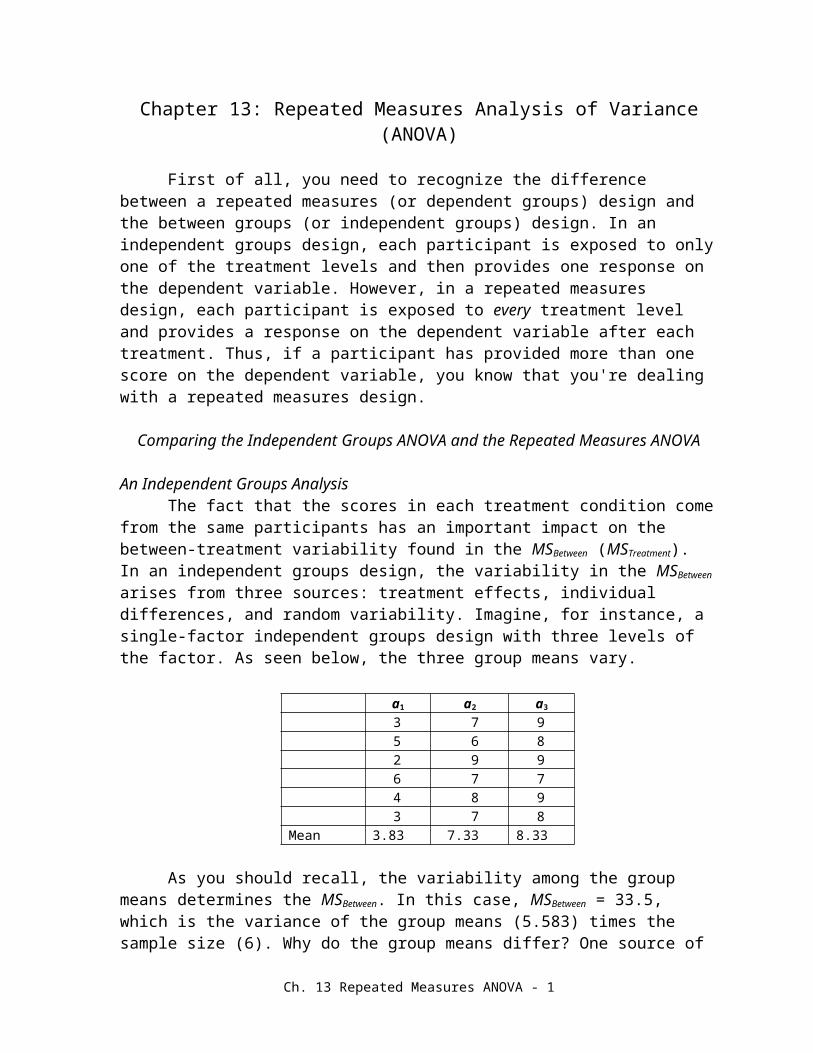
has an important impact on the between-treatment variability found in the MSBetween (MSTreatment). In an independent groups design, the variability in the MSBetween arises from three sources: treatment effects, individual differences, and random variability. Imagine, for instance, a single-factor independent groups design with three levels of the factor. As seen below, the three group means vary.

a1 a2 a3

3 7 95 6 82 9 96 7 74 8 93 7 8

Mean 3.83 7.33 8.33

As you should recall, the variability among the group means determines the MSBetween. In this case, MSBetween = 33.5, which is the variance of the group means (5.583) times the sample size (6). Why do the group means differ? One source of variability—individual differences—emerges because the scores in each group come from different people. Thus, even with random assignment to conditions, the group means could differ from one another because of individual differences. And the more variability due to individual differences in the population, the greater the variability both within groups and between groups. Another source of variability—random effects—should play a fairly small role. Nonetheless, because there will be some random variability, it could influence the three group means. Finally, you should imagine that your treatment will have an impact on the means, which is the treatment effect that you set out to examine in your experiment.

Given the sources of variability in the MSBetween, you need to construct a MSError that involves individual differences and random variability. Thus, your F-ratio would be:

F = Treatment Effect + Individual Differences + Random VariabilityIndividual Differences + Random Variability

Ch. 13 Repeated Measures ANOVA - 1

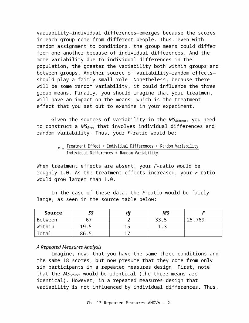
When treatment effects are absent, your F-ratio would be roughly 1.0. As the treatment effects increased, your F-ratio would grow larger than 1.0.

In the case of these data, the F-ratio would be fairly large, as seen in the source table below:

Source SS df MS FBetween 67 2 33.5 25.769Within 19.5 15 1.3Total 86.5 17

A Repeated Measures AnalysisImagine, now, that you have the same three conditions and the same 18 scores, but

now presume that they come from only six participants in a repeated measures design. First, note that the MSBetween would be identical (the three means are identical). However, in a repeated measures design that variability is not influenced by individual differences. Thus, the MSBetween of 33.5 would come from treatment effects and random effects.

In order to construct an appropriate F-ratio, you now need to develop an error term that contains only random variability. The logic of the procedure we will use is to take the error term that would be constructed were these data from an independent groups design (and would include individual differences and random variability) and remove the portion due to individual differences, which leaves behind the random variability that we want in our error term. The process is illustrated schematically in the pie charts below.

Independent Groups Repeated Measures

Conceptually, then, our F-ratio would be comprised of the components seen below:

F = Treatment Effect + Random VariabilityRandom Variability

Remember, however, that even though the components in the numerator of the F-ratio differ in the independent groups and repeated measures ANOVAs, the computations are identical. That is, regardless of the nature of the design, the formula for SSBetween is:


SSTreatment=∑ T2

n−G2

N

And the formula for dfBetween is:

df Treatment=k−1

Furthermore, you’ll still need to compute the SSWithin for the independent groups ANOVA (which is just the sum of the SS for each condition) and the dfWithin for the independent groups ANOVA (which is just n - 1 for each condition times the number of conditions). However, because this “old” error term contains both individual differences and random variability, we need to estimate and remove the contribution of individual differences.

We estimate the contribution of individual differences using the same logic as we use when computing the variability among treatments. That is, we treat each participant as the level of a factor (think of the factor as “Subject” or “Participant”). If you think of the computation this way, you’ll immediately notice that the formulas for SSBetween and SSSubject are identical, with the SSBetween working on columns while the SSSubject works on rows. The actual formula would be:

SSSubject=∑ P2

k−G2

N

If you’ll look at our data again, to complete your computation you would need to sum across each of the participants and then square those sums before adding them and dividing by the number of treatments.

a1 a2 a3 P3 7 9 195 6 8 192 9 9 206 7 7 204 8 9 213 7 8 18

Mean 3.83 7.33 8.33

Your computation of SSSubject would be:

SSSubject=192+192+202+202+212+182

3−1172

18=2287

3−760 . 5=1 . 83

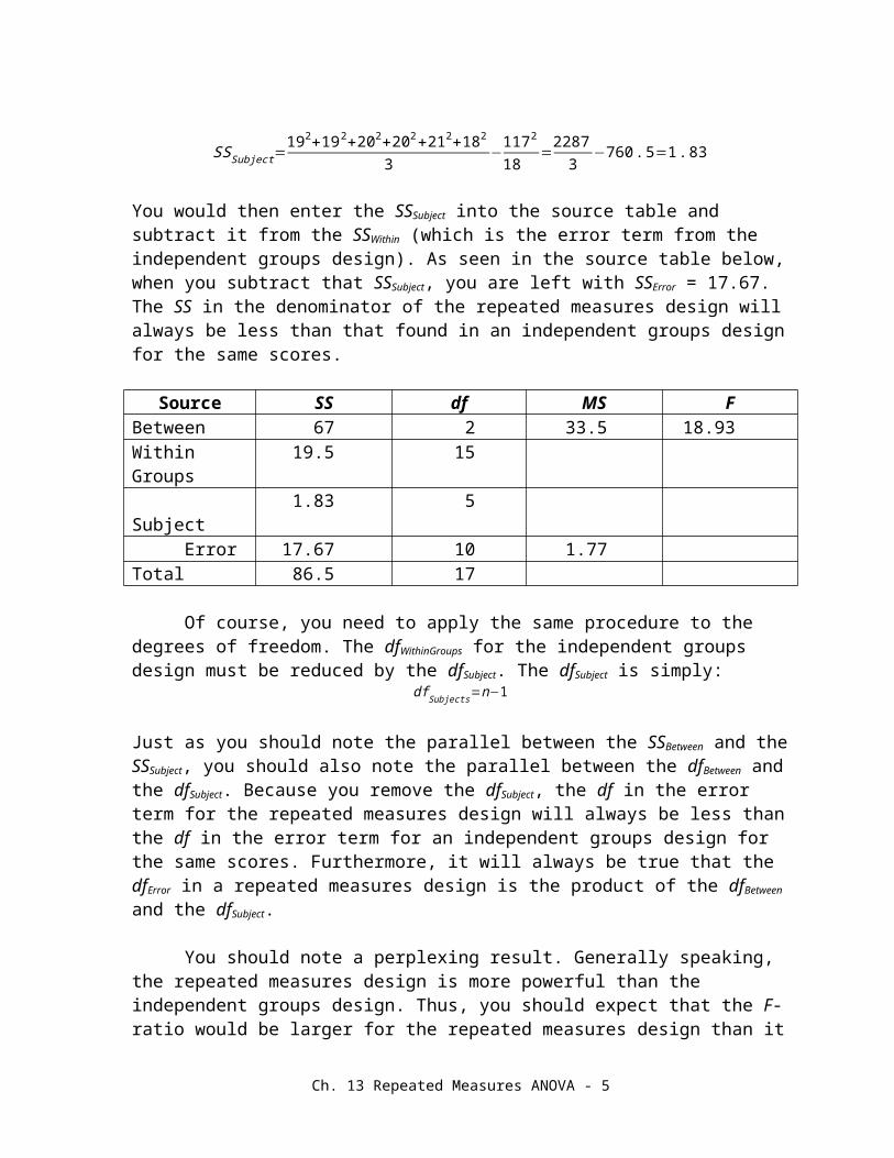
You would then enter the SSSubject into the source table and subtract it from the SSWithin (which is the error term from the independent groups design). As seen in the source table below, when you subtract that SSSubject, you are left with SSError = 17.67. The SS in the denominator of


the repeated measures design will always be less than that found in an independent groups design for the same scores.

Source SS df MS FBetween 67 2 33.5 18.93Within Groups 19.5 15 Subject 1.83 5 Error 17.67 10 1.77Total 86.5 17

Of course, you need to apply the same procedure to the degrees of freedom. The dfWithinGroups for the independent groups design must be reduced by the dfSubject. The dfSubject is simply:

df Subjects=n−1

Just as you should note the parallel between the SSBetween and the SSSubject, you should also note the parallel between the dfBetween and the dfSubject. Because you remove the dfSubject, the df in the error term for the repeated measures design will always be less than the df in the error term for an independent groups design for the same scores. Furthermore, it will always be true that the dfError in a repeated measures design is the product of the dfBetween and the dfSubject.

You should note a perplexing result. Generally speaking, the repeated measures design is more powerful than the independent groups design. Thus, you should expect that the F-ratio would be larger for the repeated measures design than it is for the independent groups design. For these data, however, that’s not the case. Note that for the independent groups ANOVA, F = 25.8 and for the repeated measures ANOVA, F = 18.9. (For the repeated measures analysis, the difference between the SPSS F and the calculator-computed F is due to rounding error.)

What happened? Think, first of all, of the formula for the F-ratio. The numerator is identical, whether the analysis is for an independent groups design or a repeated measures design. So for any difference in the F-ratio to emerge, it has to come from the denominator. Generally speaking, as seen in the formula below, larger F-ratios would come from larger dfError and smaller SSError.

F=MSTreatment

SSError

df Error

But, for identical data, the dfError will always be smaller for a repeated measures analysis! So, how does the increased power emerge? Again, for identical data, it’s also true that the SSError will always be smaller for a repeated measures analysis. As long as the SSSubject is substantial, the F-ratio will be larger for the repeated measures analysis. For these data, however, the SSSubject is actually fairly small, resulting in a smaller F-ratio. Thus, the power of the repeated measures design emerges from the presumption that people will vary. That is, you’re betting


on substantial individual differences. As you look at the people around you, that presumption is not all that unreasonable.

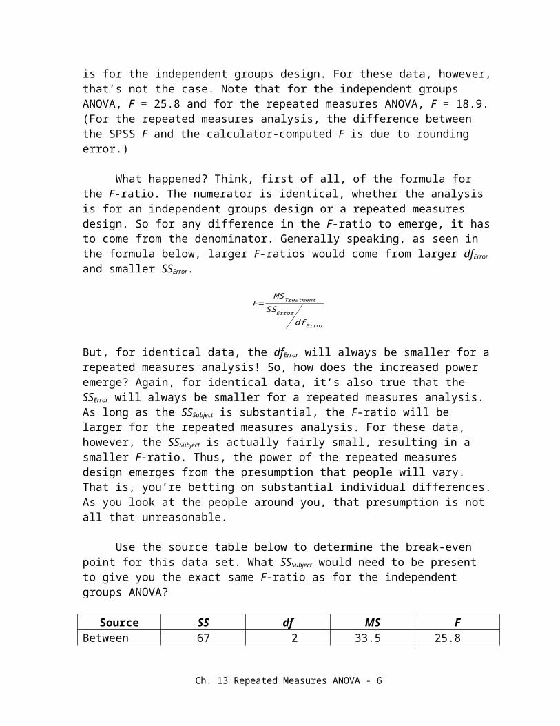
Use the source table below to determine the break-even point for this data set. What SSSubject would need to be present to give you the exact same F-ratio as for the independent groups ANOVA?

Source SS df MS FBetween 67 2 33.5 25.8Within Groups 19.5 15 Subject 5 Error 10Total 86.5 17

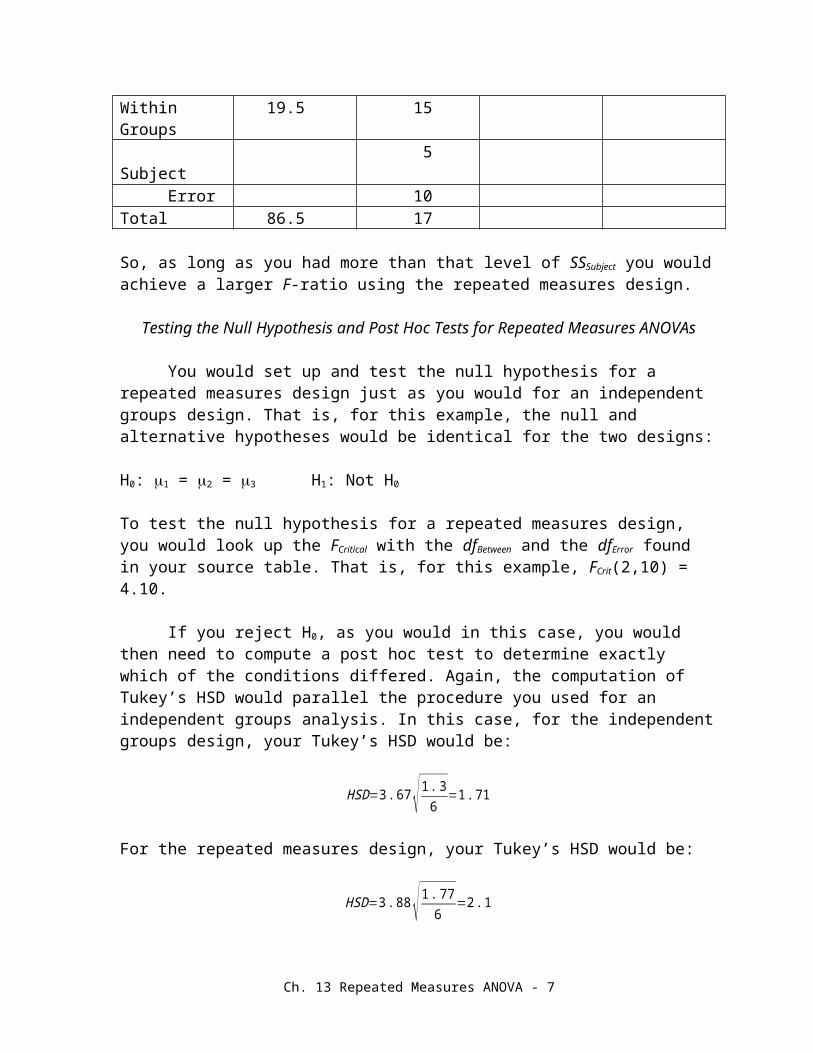
So, as long as you had more than that level of SSSubject you would achieve a larger F-ratio using the repeated measures design.

Testing the Null Hypothesis and Post Hoc Tests for Repeated Measures ANOVAs

You would set up and test the null hypothesis for a repeated measures design just as you would for an independent groups design. That is, for this example, the null and alternative hypotheses would be identical for the two designs:

H0: 1 = 2 = 3 H1: Not H0

To test the null hypothesis for a repeated measures design, you would look up the FCritical with the dfBetween and the dfError found in your source table. That is, for this example, FCrit(2,10) = 4.10.

If you reject H0, as you would in this case, you would then need to compute a post hoc test to determine exactly which of the conditions differed. Again, the computation of Tukey’s HSD would parallel the procedure you used for an independent groups analysis. In this case, for the independent groups design, your Tukey’s HSD would be:

HSD=3 .67 √ 1. 36

=1 .71

For the repeated measures design, your Tukey’s HSD would be:

HSD=3 . 88√ 1. 776

=2 .1

Ordinarily, of course, your HSD would be smaller for the repeated measures design, due to the typical reduction in the MSError. For this particular data set, given the lack of individual differences, that’s not the case.

Estimating Effect Size


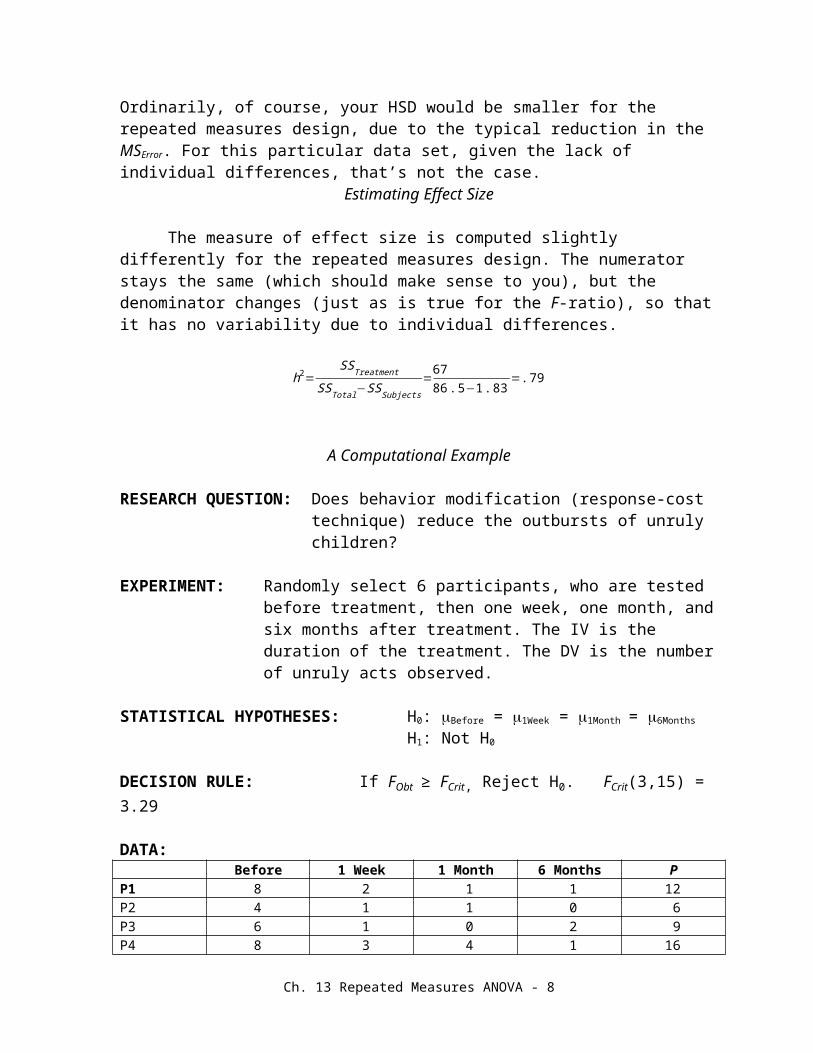
The measure of effect size is computed slightly differently for the repeated measures design. The numerator stays the same (which should make sense to you), but the denominator changes (just as is true for the F-ratio), so that it has no variability due to individual differences.

h2=SSTreatment

SSTotal−SSSubjects=67

86 . 5−1 . 83= .79

A Computational Example

RESEARCH QUESTION: Does behavior modification (response-cost technique) reduce the outbursts of unruly children?

EXPERIMENT: Randomly select 6 participants, who are tested before treatment, then one week, one month, and six months after treatment. The IV is the duration of the treatment. The DV is the number of unruly acts observed.

STATISTICAL HYPOTHESES: H0: Before = 1Week = 1Month = 6Months

H1: Not H0

DECISION RULE: If FObt ≥ FCrit, Reject H0. FCrit(3,15) = 3.29

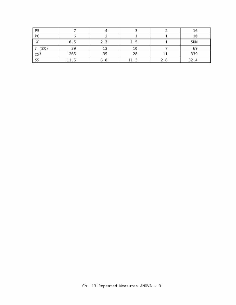
DATA:Before 1 Week 1 Month 6 Months P

P1 8 2 1 1 12P2 4 1 1 0 6P3 6 1 0 2 9P4 8 3 4 1 16P5 7 4 3 2 16P6 6 2 1 1 10X̄ 6.5 2.3 1.5 1 SUMT (X) 39 13 10 7 69X2 265 35 28 11 339SS 11.5 6.8 11.3 2.8 32.4


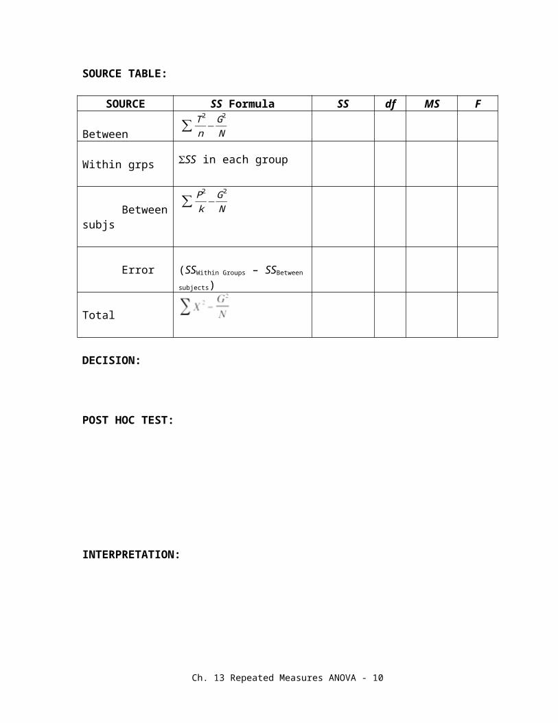
SOURCE TABLE:

SOURCE SS Formula SS df MS F

Between ∑ T 2

n− G2

N

Within grps SS in each group

Between subjs ∑ P2

k−G2

N

Error (SSWithin Groups – SSBetween subjects)

Total

DECISION:

POST HOC TEST:

INTERPRETATION:

EFFECT SIZE:


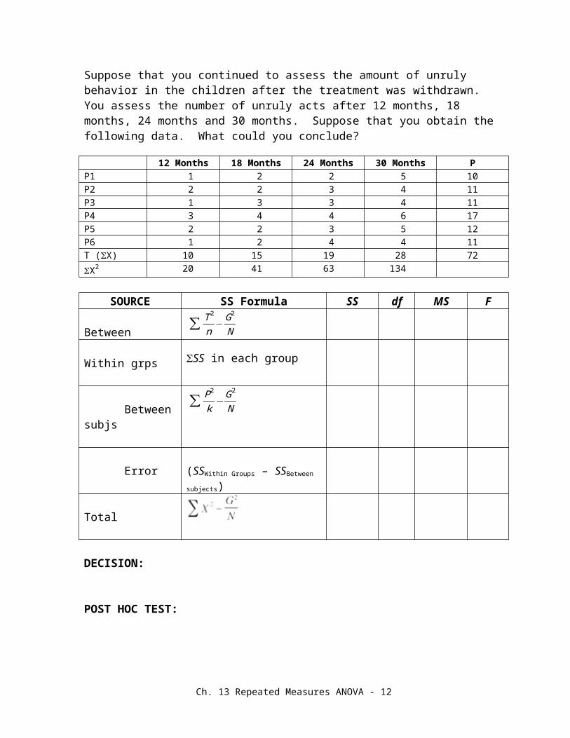
Suppose that you continued to assess the amount of unruly behavior in the children after the treatment was withdrawn. You assess the number of unruly acts after 12 months, 18 months, 24 months and 30 months. Suppose that you obtain the following data. What could you conclude?

12 Months 18 Months 24 Months 30 Months PP1 1 2 2 5 10P2 2 2 3 4 11P3 1 3 3 4 11P4 3 4 4 6 17P5 2 2 3 5 12P6 1 2 4 4 11T (X) 10 15 19 28 72X2 20 41 63 134

SOURCE SS Formula SS df MS F

Between ∑ T 2

n−G2

N

Within grps SS in each group

Between subjs ∑ P2

k−G2

N

Error (SSWithin Groups – SSBetween subjects)

Total

DECISION:

POST HOC TEST:

INTERPRETATION:

EFFECT SIZE:


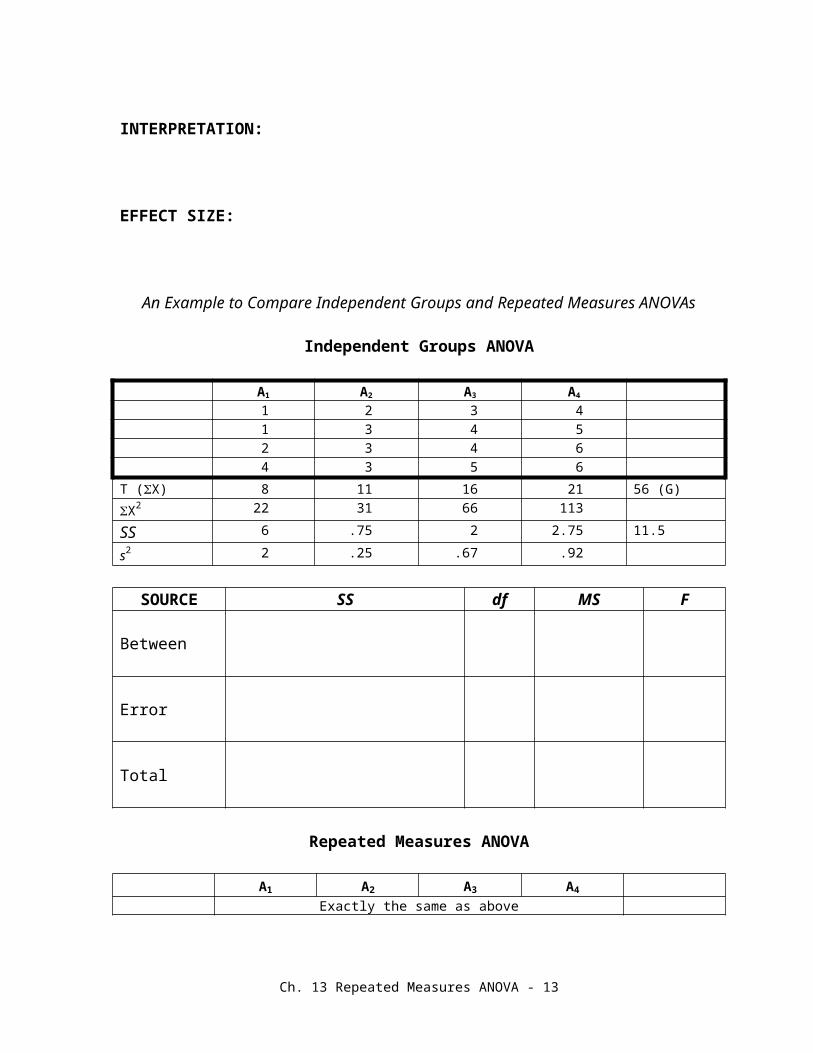
An Example to Compare Independent Groups and Repeated Measures ANOVAs

Independent Groups ANOVA

A1 A2 A3 A4

1 2 3 41 3 4 52 3 4 64 3 5 6

T (X) 8 11 16 21 56 (G)X2 22 31 66 113

SS 6 .75 2 2.75 11.5

s2 2 .25 .67 .92

SOURCE SS df MS F

Between

Error

Total

Repeated Measures ANOVA

A1 A2 A3 A4Exactly the same as above

SOURCE SS df MS F

Between

Within Groups

Between Subjs

Error

Total


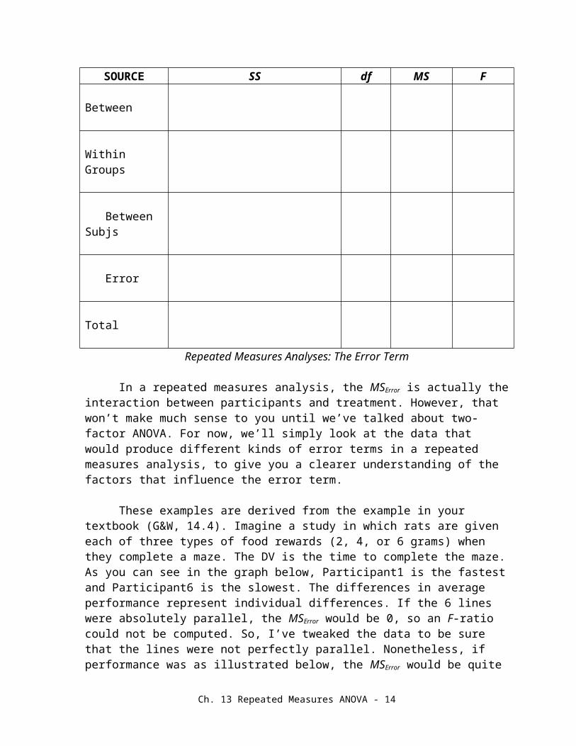
Repeated Measures Analyses: The Error Term

In a repeated measures analysis, the MSError is actually the interaction between participants and treatment. However, that won’t make much sense to you until we’ve talked about two-factor ANOVA. For now, we’ll simply look at the data that would produce different kinds of error terms in a repeated measures analysis, to give you a clearer understanding of the factors that influence the error term.

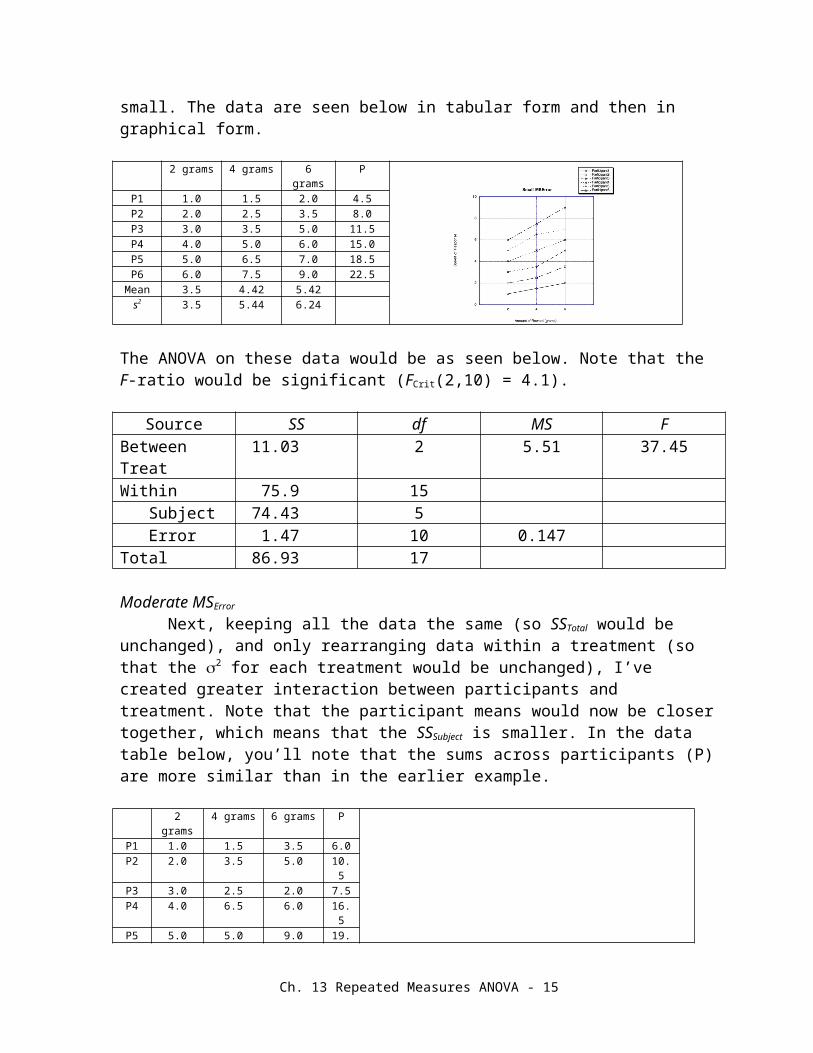
These examples are derived from the example in your textbook (G&W, 14.4). Imagine a study in which rats are given each of three types of food rewards (2, 4, or 6 grams) when they complete a maze. The DV is the time to complete the maze. As you can see in the graph below, Participant1 is the fastest and Participant6 is the slowest. The differences in average performance represent individual differences. If the 6 lines were absolutely parallel, the MSError would be 0, so an F-ratio could not be computed. So, I’ve tweaked the data to be sure that the lines were not perfectly parallel. Nonetheless, if performance was as illustrated below, the MSError would be quite small. The data are seen below in tabular form and then in graphical form.

2 grams 4 grams 6 grams PP1 1.0 1.5 2.0 4.5P2 2.0 2.5 3.5 8.0P3 3.0 3.5 5.0 11.5P4 4.0 5.0 6.0 15.0P5 5.0 6.5 7.0 18.5P6 6.0 7.5 9.0 22.5

Mean 3.5 4.42 5.42s2 3.5 5.44 6.24

The ANOVA on these data would be as seen below. Note that the F-ratio would be significant (FCrit(2,10) = 4.1).

Source SS df MS FBetween Treat 11.03 2 5.51 37.45Within 75.9 15 Subject 74.43 5 Error 1.47 10 0.147Total 86.93 17

Moderate MSError

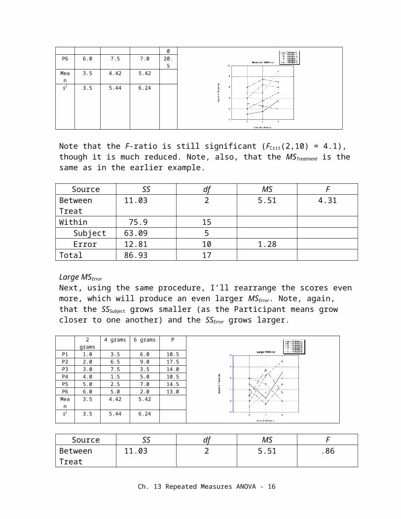
Next, keeping all the data the same (so SSTotal would be unchanged), and only rearranging data within a treatment (so that the 2 for each treatment would be unchanged), I’ve created greater interaction between participants and treatment. Note that the participant means would now be closer together, which means that the SSSubject is smaller. In the data table below, you’ll note that the sums across participants (P) are more similar than in the earlier example.

2 grams 4 grams 6 grams P


P1 1.0 1.5 3.5 6.0P2 2.0 3.5 5.0 10.5P3 3.0 2.5 2.0 7.5P4 4.0 6.5 6.0 16.5P5 5.0 5.0 9.0 19.0P6 6.0 7.5 7.0 20.5

Mean

3.5 4.42 5.42

s2 3.5 5.44 6.24

Note that the F-ratio is still significant (FCrit(2,10) = 4.1), though it is much reduced. Note, also, that the MSTreatment is the same as in the earlier example.

Source SS df MS FBetween Treat 11.03 2 5.51 4.31Within 75.9 15 Subject 63.09 5 Error 12.81 10 1.28Total 86.93 17

Large MSError

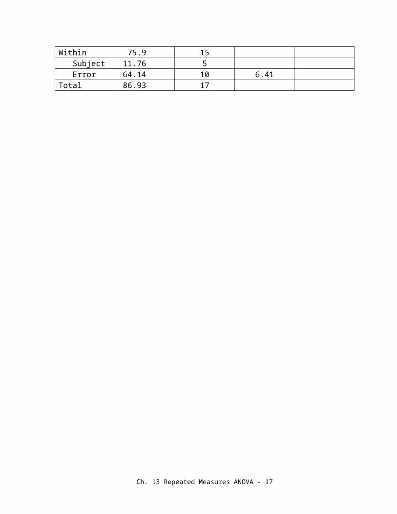
Next, using the same procedure, I’ll rearrange the scores even more, which will produce an even larger MSError. Note, again, that the SSSubject grows smaller (as the Participant means grow closer to one another) and the SSError grows larger.

2 grams 4 grams 6 grams PP1 1.0 3.5 6.0 10.5P2 2.0 6.5 9.0 17.5P3 3.0 7.5 3.5 14.0P4 4.0 1.5 5.0 10.5P5 5.0 2.5 7.0 14.5P6 6.0 5.0 2.0 13.0

Mean

3.5 4.42 5.42

s2 3.5 5.44 6.24

Source SS df MS FBetween Treat 11.03 2 5.51 .86Within 75.9 15 Subject 11.76 5 Error 64.14 10 6.41Total 86.93 17


Varying Individual Differences

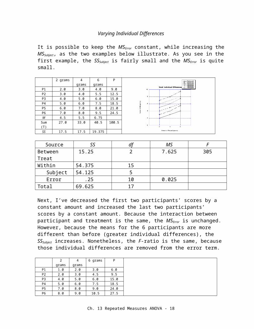
It is possible to keep the MSError constant, while increasing the MSSubject, as the two examples below illustrate. As you see in the first example, the SSSubject is fairly small and the MSError is quite small.

2 grams 4 grams 6 grams PP1 2.0 3.0 4.0 9.0P2 3.0 4.0 5.5 12.5P3 4.0 5.0 6.0 15.0P4 5.0 6.0 7.5 18.5P5 6.0 7.0 8.0 21.0P6 7.0 8.0 9.5 24.5M 4.5 5.5 6.75

Sum (T) 27.0 33.0 40.5 100.5SS 17.5 17.5 19.375

Source SS df MS FBetween Treat 15.25 2 7.625 305Within 54.375 15 Subject 54.125 5 Error .25 10 0.025Total 69.625 17

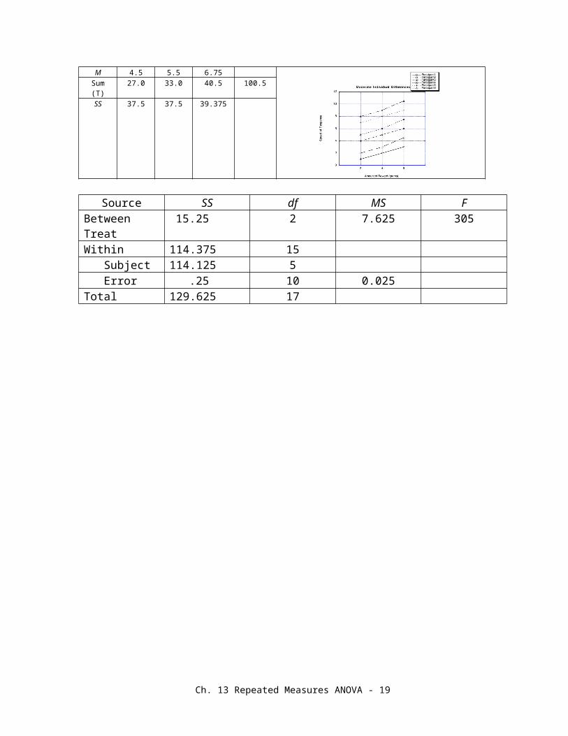
Next, I’ve decreased the first two participants’ scores by a constant amount and increased the last two participants’ scores by a constant amount. Because the interaction between participant and treatment is the same, the MSError is unchanged. However, because the means for the 6 participants are more different than before (greater individual differences), the SSSubject increases. Nonetheless, the F-ratio is the same, because those individual differences are removed from the error term.

2 grams 4 grams 6 grams PP1 1.0 2.0 3.0 6.0P2 2.0 3.0 4.5 9.5P3 4.0 5.0 6.0 15.0P4 5.0 6.0 7.5 18.5P5 7.0 8.0 9.0 24.0P6 8.0 9.0 10.5 27.5M 4.5 5.5 6.75

Sum (T) 27.0 33.0 40.5 100.5SS 37.5 37.5 39.375

Source SS df MS FBetween Treat 15.25 2 7.625 305Within 114.375 15 Subject 114.125 5 Error .25 10 0.025Total 129.625 17


SPSS for Repeated Measures ANOVA: G&W 458

First, enter as many columns (variables) as you have levels of your independent variable. Below left are the data, with each column containing scores for a particular level of the IV. For the analysis, choose General Linear Model->Repeated Measures… from the Analyze menu. Doing so will produce the window seen below right. Note that I’ve given the Within-Subject Factor Name (sleepdep) and the number of levels (3). Once I click on Add, I would click on the Define button.

The next window that appears has all your variables on the left. I’ve moved the appropriate ones to the right, as seen below left. As was true for the independent groups ANOVA, you’d probably want to know the group means, etc. Thus, you’d click on the Options… button and check the Descriptive Statistics box. As you see in the window below right, I’ve also checked the boxes for effect size and power.

Clicking on the OK button will produce the analysis seen below. The first information will be the descriptive statistics.


Next will be some output (multivariate analyses, sphericity test) that you can ignore.

Next will be the actual source table for the ANOVA. You should note the differences between the source tables that you would generate doing the analyses as shown in your Gravetter & Wallnau textbook and that generated by SPSS. Note that SPSS doesn’t show the Subject effect, but just the Treatment effect (A) and the Error term.

The source table appears to be relatively complicated, but you can simplify the output with the proper focus. First, note that there are two basic rows of interest: the Treatment row (sleepdep) containing the F-ratio and the Error row. You can ignore the lower three lines (Greenhouse-Geisser, Huynh-Feldt, and Lower-bound). For instance, for our purposes, you can focus entirely on the Sphericity Assumed line.

Finally, there are some other parts of the output that you can ignore, as seen below:


Practice Problems

Drs. Dewey, Stink, & Howe were interested in memory for various odors. They conducted a study in which 6 participants were exposed to 10 common food odors (orange, onion, etc.) and 10 common non-food odors (motor oil, skunk, etc.) to see if people are better at identifying one type of odorant or the other. The 20 odors were presented in a random fashion, so that both classes of odors occurred equally often at the beginning of the list, at the end of the list, etc. (Thus, this randomization is a strategy that serves the same function as counterbalancing.) The dependent variable is the number of odors of each class correctly identified by each participant. The data are seen below. Analyze the data and fully interpret the results of this study.

Food Odors Non-Food Odors7 48 66 49 77 55 3

X (T) 42 29X2 304 151SS 10 10.8


Suppose that Dr. Belfry was interested in conducting a study about the auditory capabilities of bats, looking at bats’ abilities to avoid wires of varying thickness as they traverse a maze. The DV is the number of times that the bat touches the wires. (Thus, higher numbers indicate an inability to detect the wire.) Complete the source table below and fully interpret the results.


Dr. Richard Noggin is interested in the effect of different types of persuasive messages on a person’s willingness to engage in socially conscious behaviors. To that end, he asks his participants to listen to each of four different types of messages (Fear Invoking, Appeal to Conscience, Guilt, and Information Laden). After listening to each message, the participant rates how effective the message was on a scale of 1-7 (1 = very ineffective and 7 = very effective). Complete the source table and analyze the data as completely as you can.


Dr. Beau Peep believes that pupil size increases during emotional arousal. He was interested in testing if the increase in pupil size was a function of the type of arousal (pleasant vs. aversive). A random sample of 5 participants is selected for the study. Each participant views all three stimuli: neutral, pleasant, and aversive photographs. The neutral photograph portrays a plain brick building. The pleasant photograph consists of a young man and woman sharing a large ice cream cone. Finally, the aversive stimulus is a graphic photograph of an automobile accident. Upon viewing each photograph, the pupil size is measured in millimeters. An incomplete source table resulting from analysis of these data is seen below. Complete the source table and analyze the data as completely as possible.


In PS 306, we conducted a lab in which subjects served as mock eyewitnesses. Even though they hadn’t actually observed a crime, they could read descriptions from eyewitnesses (see below) and then rate the similarity of each of the six pictures in a photo-array (see below) to that description. Think about it. If the police put together an unbiased photo-array, what should happen? Right! People should rate all the faces as equally similar to the eyewitness description. In other words, if the photo-array was fair, an analysis of the data would retain H0: Face1

= Face2 = Face3 = Face4 = Face5 = Face6. If the similarity ratings (made on a 7-pt scale, from 1 = bad match to 7 = great match) differ for the faces, it would indicate that the photo-array is biased. Complete the analysis below and interpret the results as completely as you can. (A1F1 means Array 1 Face 1, etc.) [N.B. The photos were presented simultaneously, so there was no counterbalancing.]

African-American male in his early 20’s with dark hair, an oval face and broad forehead. Small, dark eyes and thin eyebrows. A wide nose, thick lips and small, protruding ears.

Source Type III Sum of Squares df

Mean Square F Sig.

Partial Eta Squared

Observed Powera

face Sphericity Assumed 579.1 .000 .450 1.000

Error(face) Sphericity Assumed 707.9


As before, given that old exams use StatView, here is an example of a repeated measures analysis in StatView. Note that there are several differences between the SPSS output and StatView output (reversal of df and SS columns, inclusion of a row for the Subject effect).

Suppose you are interested in studying the impact of duration of exposure to faces on the ability of people to recognize faces. To finesse the issue of the actual durations used, I'll call them Short, Medium, and Long durations. Participants are first exposed to a set of 30 faces for one duration and then tested on their memory for those faces. Then they are exposed to another set of 30 faces for a different duration and then tested. Finally, they are given a final set of 30 faces for the final duration and then tested. The DV for this analysis is the percent Hits (saying Old to an Old item). Suppose that the results of the experiment come out as seen below. Complete the analysis and interpret the results as completely as you can. If the results turned out as seen below, what would they mean to you?


chapter 13: introduction to analysis of varianceskidmore.edu/~hfoley/handouts/s.ch13.docx · web...

Documents