Repeated Measures

Chapter 13

Chapter Objectives

• Rationale of Repeated Measures ANOVA– One- and two-way– Benefits

• Partitioning Variance• Statistical Problems with Repeated Measures

Designs– Sphericity– Overcoming these problems

• Interpretation

Benefits of Repeated Measures Designs

• Sensitivity–Unsystematic variance is reduced.–More sensitive to experimental effects.–More powerful than independent designs

• Economy– Less participants are needed.–But, be careful of fatigue.

Problems with Repeated Measures Designs

• Same participants in all conditions.– Scores across conditions correlate.– Violates assumption of independence.

• Assumption of Sphericity.– Crudely put: the correlation across conditions

should be the same.– The variance of the differences of each pair must

be equal.

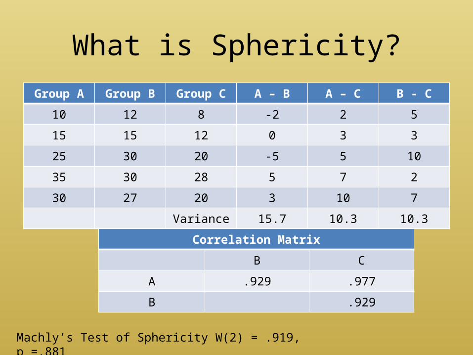
What is Sphericity?Group A Group B Group C A – B A – C B - C

10 12 8 -2 2 5

15 15 12 0 3 3

25 30 20 -5 5 10

35 30 28 5 7 2

30 27 20 3 10 7

Variance 15.7 10.3 10.3

Correlation Matrix

B C

A .929 .977

B .929

Machly’s Test of Sphericity W(2) = .919, p =.881

Effects of a 6 Week Agility Training Program

• 8 subjects were pre-tested for agility.• The subjects then participated in a 6 week agility

training program.• Their agility was measured at the following time

points: Pre, 3 weeks, 6 weeks, and a 3 week follow up.

• A single factor repeated measures ANOVA with one within-subjects factor Time (pre, 3 weeks, 6 weeks, follow-up) was used to determine the effects of the training program on agility.

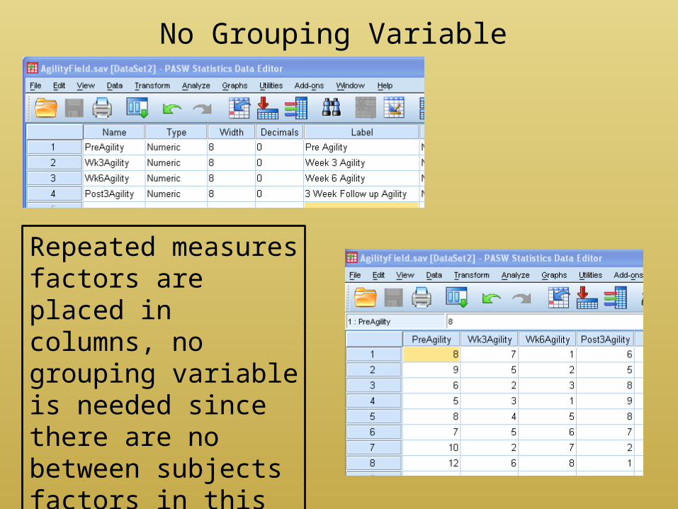
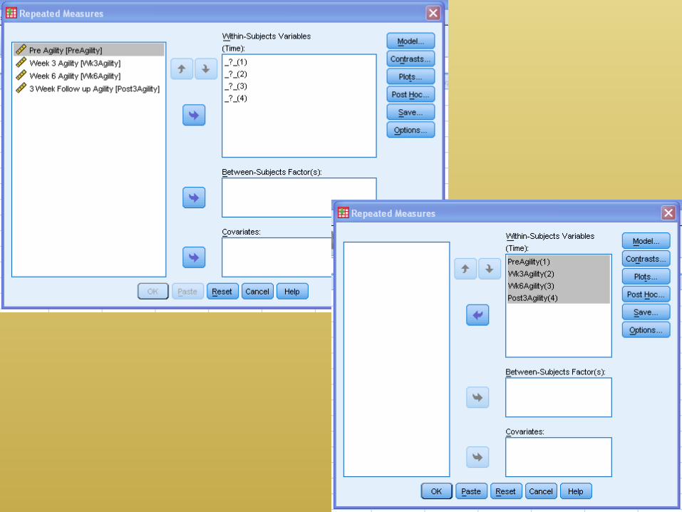
No Grouping Variable

Repeated measures factors are placed in columns, no grouping variable is needed since there are no between subjects factors in this experiment.

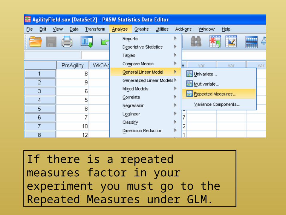
If there is a repeated measures factor in your experiment you must go to the Repeated Measures under GLM.

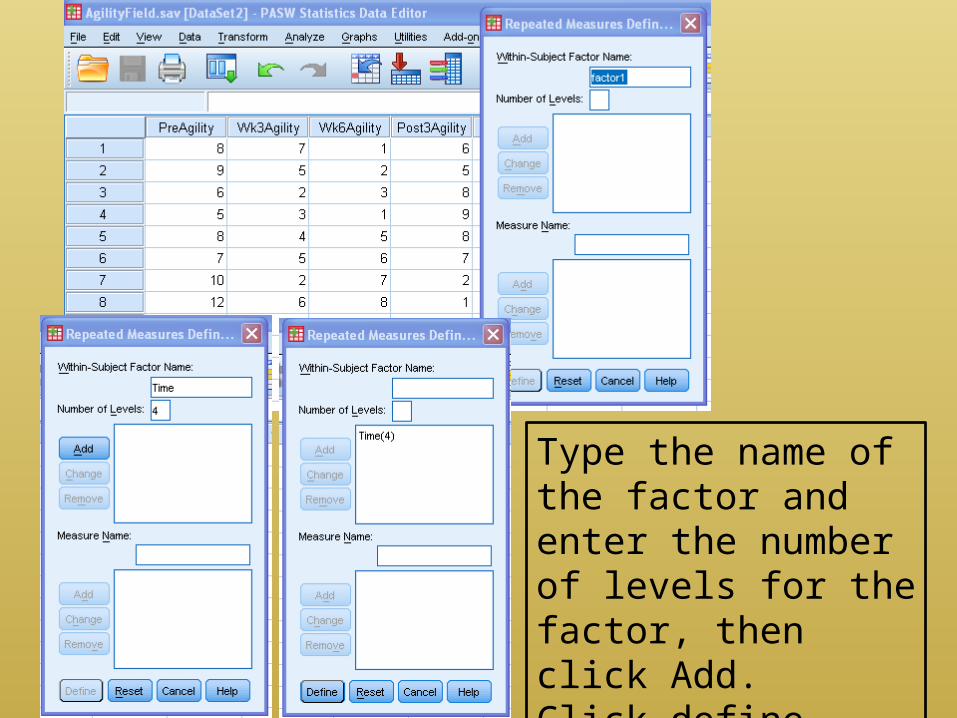
Type the name of the factor and enter the number of levels for the factor, then click Add.Click define.

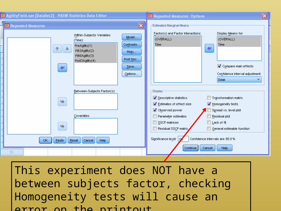
This experiment does NOT have a between subjects factor, checking Homogeneity tests will cause an error on the printout.

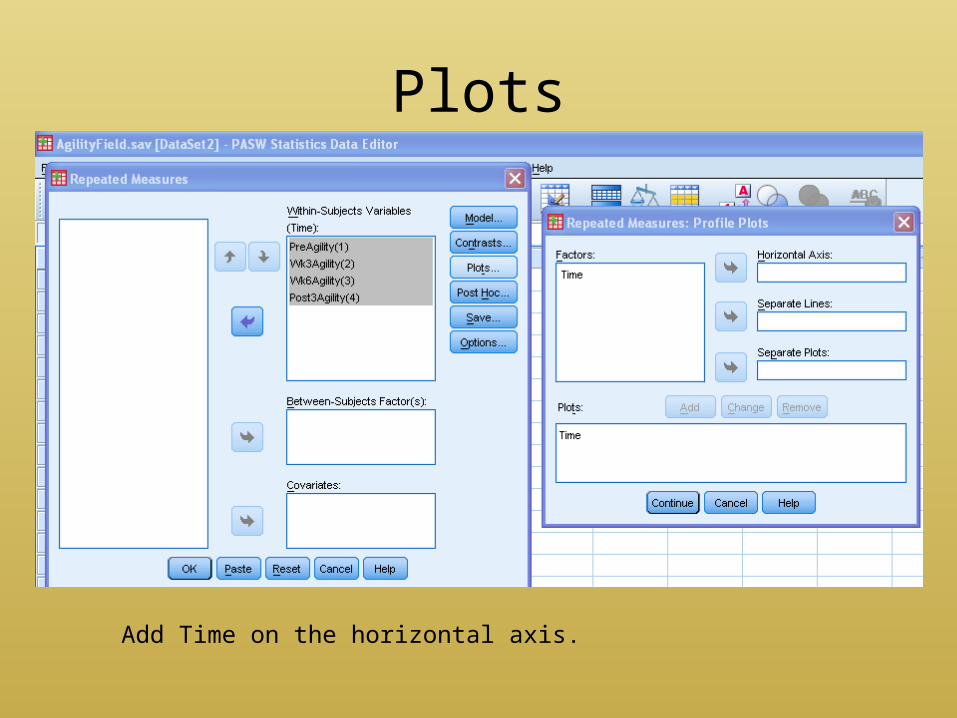
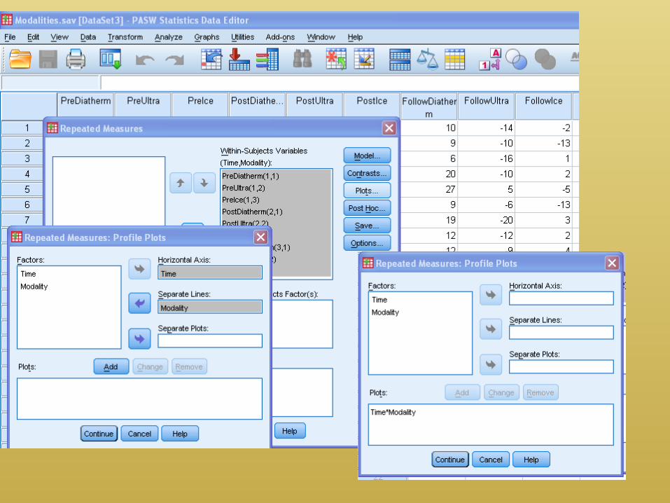
Plots

Add Time on the horizontal axis.

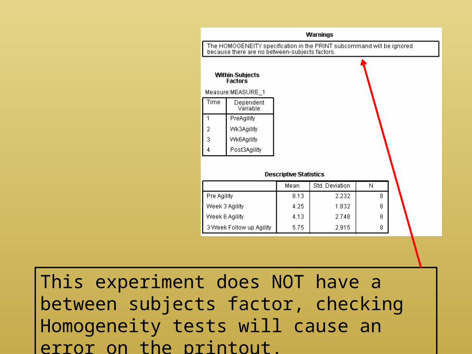
This experiment does NOT have a between subjects factor, checking Homogeneity tests will cause an error on the printout.

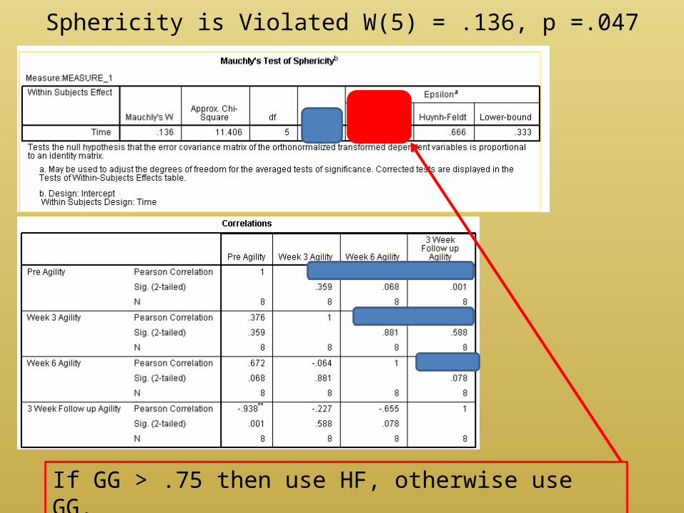
Sphericity is Violated W(5) = .136, p =.047

If GG > .75 then use HF, otherwise use GG.

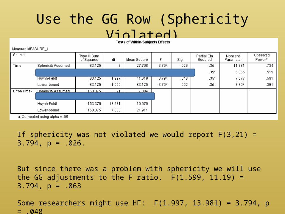
Use the GG Row (Sphericity Violated)

If sphericity was not violated we would report F(3,21) = 3.794, p = .026.

But since there was a problem with sphericity we will use the GG adjustments to the F ratio. F(1.599, 11.19) = 3.794, p = .063

Some researchers might use HF: F(1.997, 13.981) = 3.794, p = .048

3x3 With Two Within Subjects Factors

The purpose of this experiment was to test the effects of diathermy, ultrasound and ice on joint stiffness. Twenty subjects with arthritis received treatments in all three conditions (diathermy, ultrasound and ice). The order of treatment was counterbalanced. The subjects joint stiffness was measured at the following time points for each treatment: pre, post and followup.

A 3 x 3 repeated measures ANOVA with two within-subjects factors treatment (diathermy, ultrasound, ice) and time (pre, post, follow up) was used to compare the effects of the treatments on joint stiffness.

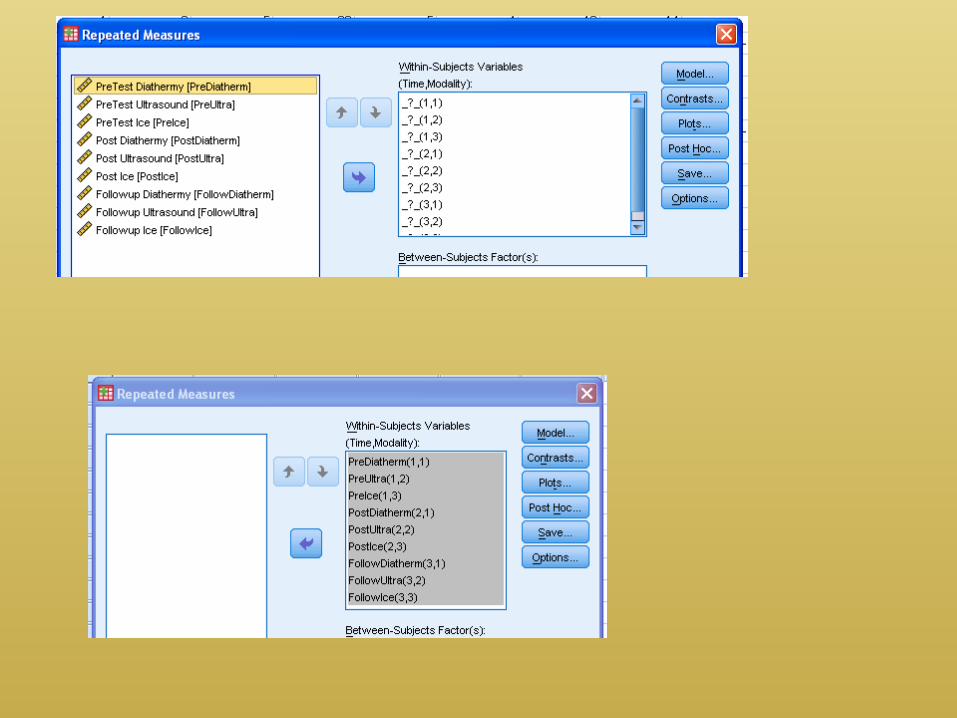
3 x 3 Within – Within Design

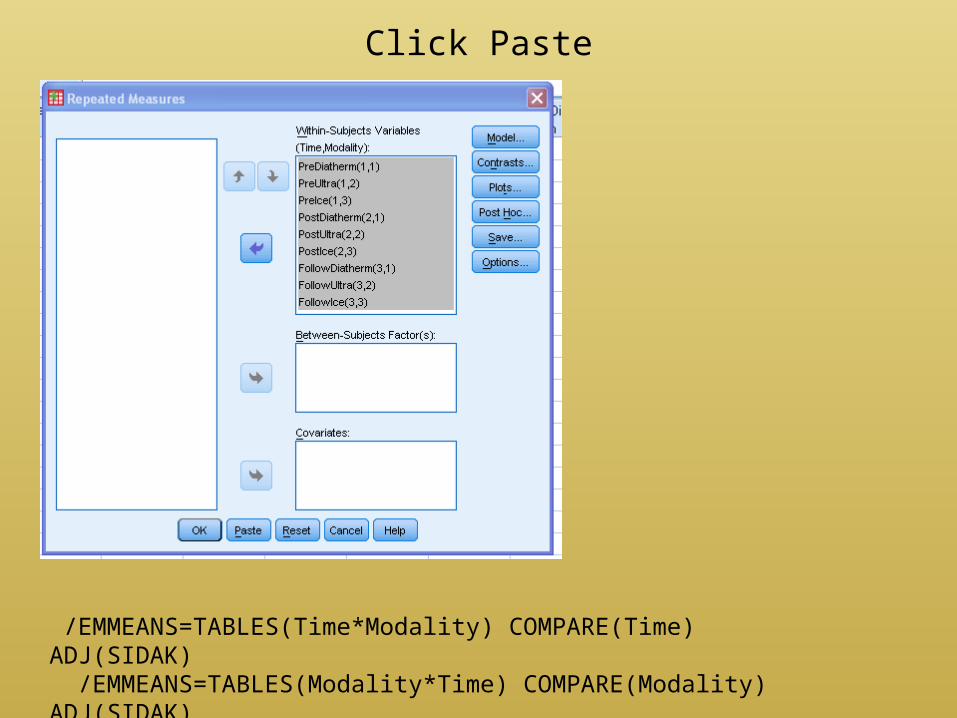
Click Paste

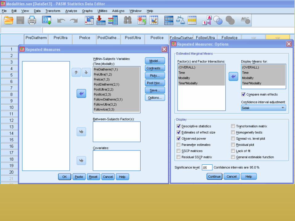
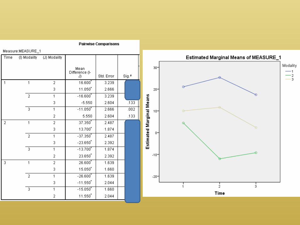
/EMMEANS=TABLES(Time*Modality) COMPARE(Time) ADJ(SIDAK) /EMMEANS=TABLES(Modality*Time) COMPARE(Modality) ADJ(SIDAK)

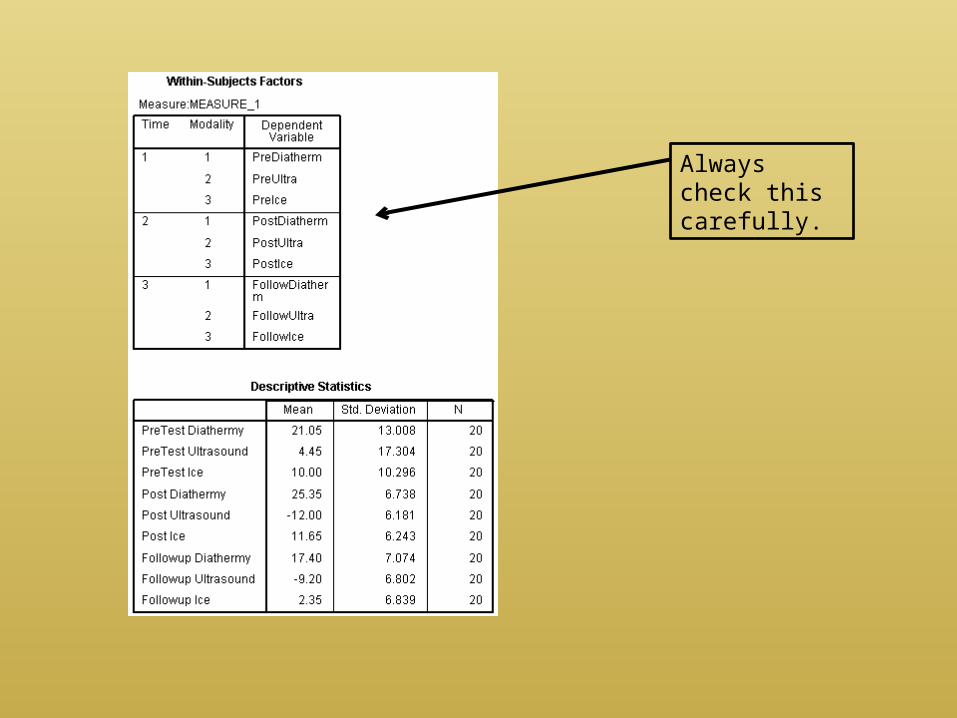
Always check this carefully.

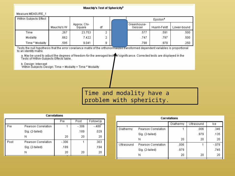
Time and modality have a problem with sphericity.

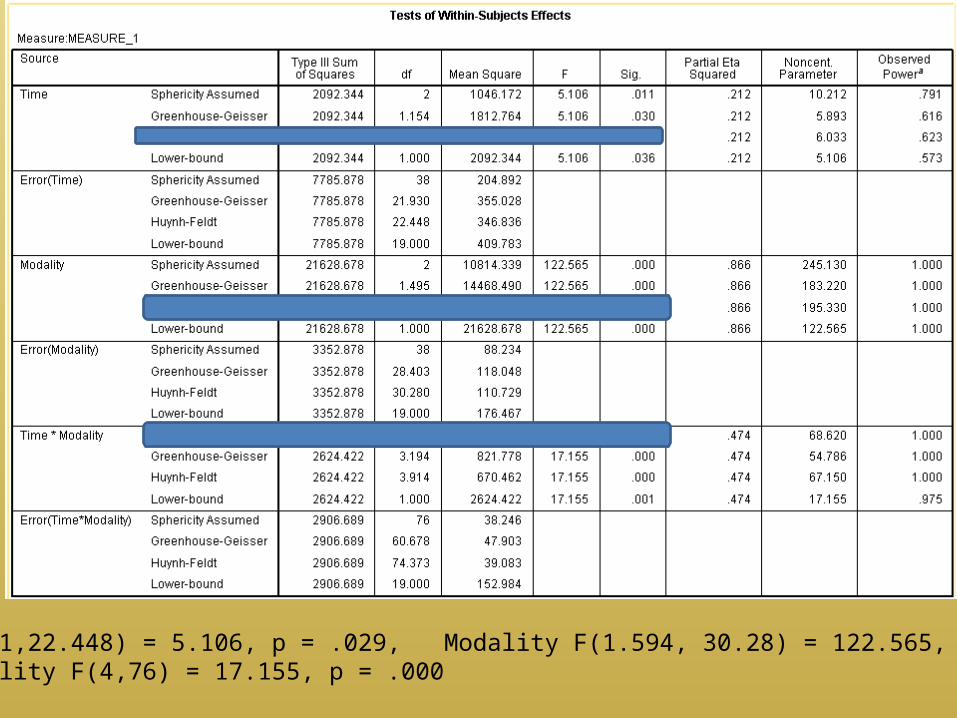
Time F(1.181,22.448) = 5.106, p = .029, Modality F(1.594, 30.28) = 122.565, p = .000Time x Modality F(4,76) = 17.155, p = .000

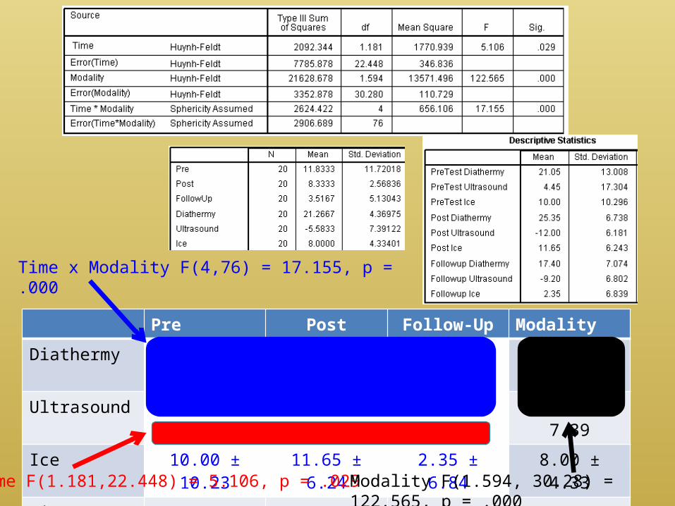
Pre Post Follow-Up Modality

Diathermy 21.05 ± 13.01 25.35 ± 6.74 17.40 ± 7.07 21.27 ± 4.37

Ultrasound 4.45 ± 17.30 -12.00 ± 6.18 -9.20 ± 6.80 -5.58 ± 7.39

Ice 10.00 ± 10.23 11.65 ± 6.24 2.35 ± 6.84 8.00 ± 4.33

Time Means 11.83 ± 11.72 8.33 ± 2.57 3.52 ± 5.13

Time F(1.181,22.448) = 5.106, p = .029 Modality F(1.594, 30.28) = 122.565, p = .000

Time x Modality F(4,76) = 17.155, p = .000

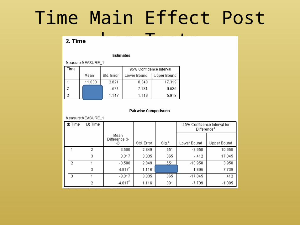
Time Main Effect Post hoc Tests

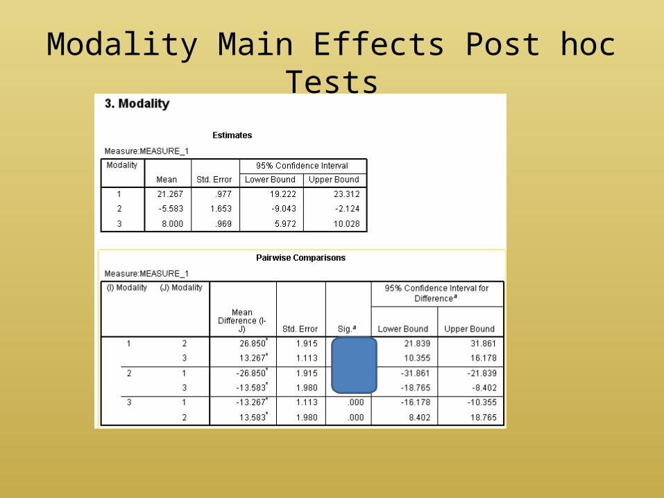
Modality Main Effects Post hoc Tests

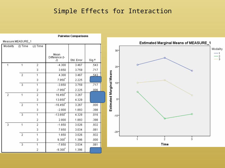
Simple Effects for Interaction

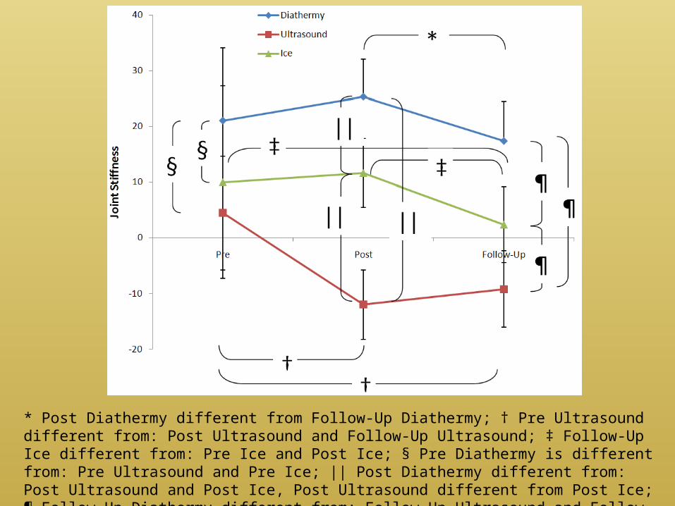
* Post Diathermy different from Follow-Up Diathermy; † Pre Ultrasound different from: Post Ultrasound and Follow-Up Ultrasound; ‡ Follow-Up Ice different from: Pre Ice and Post Ice; § Pre Diathermy is different from: Pre Ultrasound and Pre Ice; || Post Diathermy different from: Post Ultrasound and Post Ice, Post Ultrasound different from Post Ice; ¶ Follow-Up Diathermy different from: Follow-Up Ultrasound and Follow-Up Ice, Follow-Up Ultrasound different from Follow-Up Ice; p < 0.05.

HomeworkAnalyze the Task 1 the book (TutorMarks.sav), see page 504.

Analyze Experiment 3.Do a Sidak post hoc test instead of the planned contrast suggested in the book.

Use simple effects testing for a significant interaction.

Use the Sample Methods and Results section as a guide to write a methods and results section for your homework.