3. Fluid Dynamics

Blood Circuit

BK

3.1 Medical reference and goal of the experiment

The behaviour of fluid currents is described by the theory of fluid dynamics. It is the foundation

for the description of the blood circulation in the human body.

Lung

Rightheart

ventricle

Brain,liver,stomach,intestine,muscles

....

Leftheart

ventricle

Abbildung 3.1: Schematic representation of the human blood circuit.

In the blood circuit (Fig. 3.1), blood serves as a drifting medium for the transport of O2, CO2 and

other substances. The whole human circulation system consists of the smaller pulmonary(lungs),

as well as the bigger systemic circulation, both which are cascaded one after the other from birth

on. In the pulmonary-circuit, oxygen-deficient blood is being pumped from the right ventricle

(heart chamber) through the lungs, where CO2 is being released and the blood gets enriched with

O2, before it reaches the right atrial. Valve flaps ensure that a directed current is being created

and maintained. The vascular system includes arteries, arterioles, capillaries, venules and veins in

serial connection. The supply of the individual organs is provided by a highly branched parallel

1

2 Fluid Dynamics

arrangement of blood vessels. The elastic venous system and the right atrium form a blood reservoir,

from which the blood flows back to the heart.

For this experiment a circular flow model, representing the human blood circuit, has been developed.

The heart is being replaced by a single piston pump. The fluid (paraffin oil is being used), flows

through a simplistic vascular system, which consists of pipes of various lengths and diameters.

With the help of the model one can study the fundamental function of a circulatory system and

the relevance of its individual components. For a periodically working pump in particular, you will

study the influence of a so-called air vessel on the pressure and current conditions. In the human

circulation system this function is mainly undertaken by the stretchable aorta.

The fundamentals of fluid dynamics, which you acquire through the example of the blood circuit,

are also valid in a wide range for the alveolar ventilation, the transportation of breathing gas

between the alveoli and the environment. The moving medium in that case is the breathing gas,

which flows through the respiratory tract due to pressure differences.

Note: For this experiment it is highly recommended to bring coloured pencils with you.

3.2 Experimental part

3.2.1 Functional principle of the circuit model and air vessel

Running without air vessel

First, you should acquaint yourself with the components of the circuit model and their meaning

for the functionality of the model.

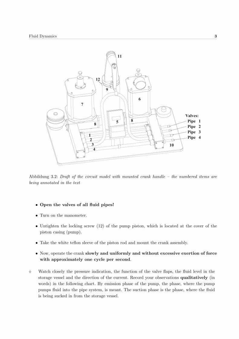
The components are (Numbers cf. Fig. 3.2):

– a pump (9) with 2 valve flaps (8), on which, for periodic operation, a crank handle (11) has

to be mounted,

– an air vessel (6), whose functionality is not being used until the next measurement and

therefore remains closed for the moment,

– various current pipes (1 to 4), which can be locked individually via valves (10),

– a storage vessel (7), into which the fluid from the pipe system flows into, before being sucked

in by the pump again,

– a manometer (5), which indicates the pressure difference ∆p in the fluid, i.e. the difference of

pressure between the starting and end points of pipes

The functionality of the individual components can be understood best when the device is in slow

periodic operation. The following tasks will be performed together with the assistant on

a demonstration model.

• The manometer has to be connected to the power supply. The scale indicates the pressure

difference ∆p in hPa (Full-scale deflection: 100 hPa).

Fluid Dynamics 3

1234

67

9

11

12

885

10

Valves: Pipe 1 Pipe 2 Pipe 3 Pipe 4

Abbildung 3.2: Draft of the circuit model with mounted crank handle – the numbered items are

being annotated in the text

• Open the valves of all fluid pipes!

• Turn on the manometer.

• Untighten the locking screw (12) of the pump piston, which is located at the cover of the

piston casing (pump).

• Take the white teflon sleeve of the piston rod and mount the crank assembly.

• Now, operate the crank slowly and uniformly and without excessive exertion of force

with approximately one cycle per second.

� Watch closely the pressure indication, the function of the valve flaps, the fluid level in the

storage vessel and the direction of the current. Record your observations qualitatively (in

words) in the following chart. By emission phase of the pump, the phase, where the pump

pumps fluid into the pipe system, is meant. The suction phase is the phase, where the fluid

is being sucked in from the storage vessel.

4 Fluid Dynamics

Suction phase Emission phase

Pressure Difference

Position of the left valve flap

Position of the left valve flap

Fluid Level in the storage vessel

Direction of current in pipes

� What are the requirements, for that a flow occurs inside the pipe system? What is the storage

vessel necessary for?

� Which components ensure the rectification of the current and which are their anatomical

correspondents?

Pressure fluctuations in the pipe system without air vessel

� Double-check, that all valves are still open and the air vessel (6) is closed (screw on top

completely screwed in clockwise - without exertion of force!). Now turn the crank with

approx. one turn per second. Thereby the difference ∆p of pressures in front of the pipes and

behind them changes periodically. Read out the minimum (∆pmin) and maximum (∆pmax)

value, which the pressure difference takes on during a pumping cycle (units!):

without air vessel: ∆pmin ≈ ∆pmax ≈

Fluid Dynamics 5

Running with air vessel

� Open the air vessel (6), by unscrewing the screw in the cover of the air vessel clockwise.

Just like before, turn the crank. What qualitative changes do you observe, compared to the

running without the air vessel? In doing so, also take into account the behaviour of the fluid

inside the air vessel.

� From the pressure indication on the air vessel you can read off the pressure over the fluid in

the air vessel. What happens to the air during the suction and emission phase?

Pressure fluctuations in the pipe system with air vessel

� Again, measure the minimum and maximum pressure difference, that occurs during one

pumping cycle. (Here it is important, to crank roughly with the same rhythm like you did

for the measurements without air vessel.)

with air vessel: ∆pmin ≈ ∆pmax ≈

Comparison of measurements with and without air vessel

� Register the measured pressure differences as crossbars with different colours for the measu-

rements without and with air vessel in the following scale:

(Windkessel means air vessel)

140120100806040200Maximum and minimum pressure values [hPa]

Without “Windkessel”:

Using the “Windkessel”:

6 Fluid Dynamics

� How does the air vessel influences the occurring pressure differences and the behaviour of

the currents and why is this of importance for the blood circuit? (How is this functionality

implemented in the human body?)

• Release the piston by setting it to the highest position possible, removing the pivot between

crank handle and piston and reinstalling the teflon sleeve. This prevents oil from rising above

the piston.

• Lock up the air vessel by closing the valve by hand, turning it clockwise.

3.2.2 Flow behaviour of fluids

In this section, further investigation on the correlation of pressure difference and flow behaviour is

being undertaken. For the description of the flow behaviour you have to determine the volumetric

flow rate I . It specifies the ratio of a volume element ∆V of the fluid that passes a cross section

of the pipe and the period of time ∆t it takes to do so.1:

I =∆V

∆t.

• To examine the correlation of pressure difference and volumetric flow rate systematically,

running the device in a periodical manner is inappropriate due to the permanent pressure

fluctuations. Therefore, you will only work with the piston and weight plates.

• Furthermore, for the time being, the fluid should flow through one pipe at a time only.

Therefore, close the pipes 1, 3 and 4 with the valves and open pipe 2.

For the determination of the pressure difference ∆ p, once again the manometer is used:

You now have the possibility to apply a constant pressure on the piston by laying on some weight

plates and therefore letting it drop a predefined distance.

Caution: It is forbidden to push down the piston by hand violently or to pull up

the piston violently because that causes the apparatus to become leaky. For the same

reasons, weight plates are only allowed to lay on the piston during the measurement

and have to be taken away during measurement pauses.

1In this experiment we will often use the unit mm instead of the SI-unit m, e.g. the unit of a volume element is

mm3 respectively. Take this into account for further calculations!

Fluid Dynamics 7

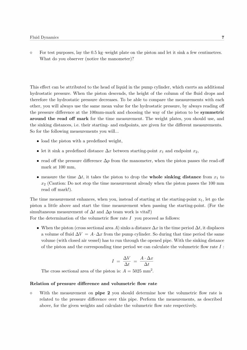
� For test purposes, lay the 0.5 kg–weight plate on the piston and let it sink a few centimetres.

What do you observer (notice the manometer)?

This effect can be attributed to the head of liquid in the pump cylinder, which exerts an additional

hydrostatic pressure. When the piston descends, the height of the column of the fluid drops and

therefore the hydrostatic pressure decreases. To be able to compare the measurements with each

other, you will always use the same mean value for the hydrostatic pressure, by always reading off

the pressure difference at the 100mm-mark and choosing the way of the piston to be symmetric

around the read off mark for the time measurement. The weight plates, you should use, and

the sinking distances, i.e. their starting- and endpoints, are given for the different measurements.

So for the following measurements you will...

• load the piston with a predefined weight,

• let it sink a predefined distance ∆x between starting-point x1 and endpoint x2,

• read off the pressure difference ∆p from the manometer, when the piston passes the read-off

mark at 100 mm,

• measure the time ∆t, it takes the piston to drop the whole sinking distance from x1 to

x2 (Caution: Do not stop the time measurement already when the piston passes the 100 mm

read off mark!).

The time measurement enhances, when you, instead of starting at the starting-point x1, let go the

piston a little above and start the time measurement when passing the starting-point. (For the

simultaneous measurement of ∆t and ∆p team work is vital!)

For the determination of the volumetric flow rate I you proceed as follows:

• When the piston (cross sectional area A) sinks a distance ∆x in the time period ∆t, it displaces

a volume of fluid ∆V = A ·∆x from the pump cylinder. So during that time period the same

volume (with closed air vessel) has to run through the opened pipe. With the sinking distance

of the piston and the corresponding time period we can calculate the volumetric flow rate I :

I =∆V

∆t=

A · ∆x

∆t

The cross sectional area of the piston is: A = 5025 mm2.

Relation of pressure difference and volumetric flow rate

� With the measurement on pipe 2 you should determine how the volumetric flow rate is

related to the pressure difference over this pipe. Perform the measurements, as described

above, for the given weights and calculate the volumetric flow rate respectively.

8 Fluid Dynamics

Measurement on pipe 2

m [kg] 2.0 1.5 1.0

x1 [mm] 60 70 80

x2 [mm] 140 130 120

∆x [mm] 80 60 40

∆p [hPa]

∆t [s]

I [104 mm3 s-1]

• Now unload the piston, pull it a little bit upwards and lock it with a clamp.

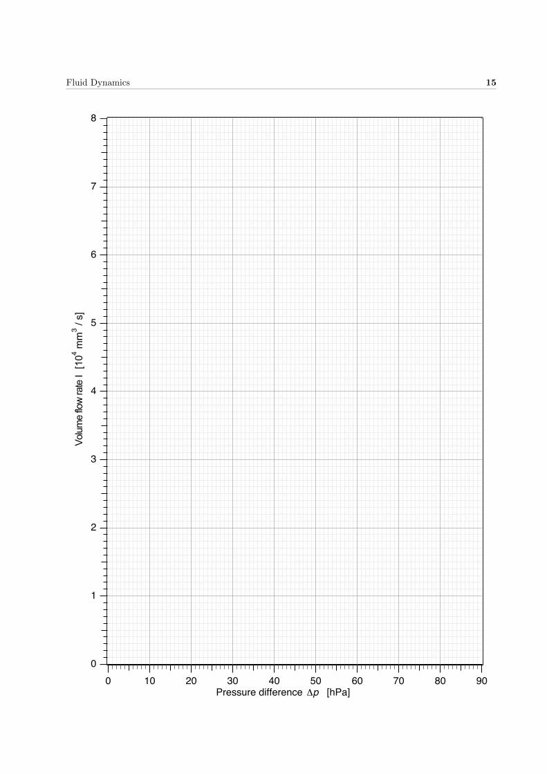
� Fill in the values for ∆p and I into the table on page 14 and plot the volumetric flow rate

against the pressure difference in the diagram on page 15.

� What kind of relation do you expect between those two quantities, based the information you

can extract from the diagram?

� Now, determine the slope of the straight line with help of a slope triangle.

The slope indicates the conductance G of the resistance pipe, through which the fluid streams.

From G, calculate the flow resistance R as the inverse of G (pay attention to the units!):

Pipe 2

G2 =

R2 =

Dependence of the flow resistance from the length of the pipe

With this measurement you will examine the relation between the length of the pipe and its flow

resistance.

� As to that you perform the same measurement on pipe 3, which is approximately double the

length of pipe 2 (while having the same diameter). For this measurement, you have to close

the valves for the pipes 1, 2 and 4.

Fluid Dynamics 9

Measurement on pipe 3

m [kg] 2.0 1.5 1.0

x1 [mm] 68 76 84

x2 [mm] 132 124 116

∆x [mm] 64 48 32

∆p [hPa]

∆t [s]

I [104 mm3 s-1]

• Unload and lock the piston again.

� Again, fill in the values for ∆p and I into the table on page 14 and plot the volumetric flow

rate against the pressure difference in another colour in the diagram on page 15. Determine

the conductance and the flow resistance of pipe 3.

Pipe 3

G3 =

R3 =

� Compare your results to those from pipe 2, which has the same diameter but is only about

half as long as pipe 3. What kind of relation (proportional, exponential, ...) do you expect

between the flow resistance and the length of the pipe?

� One could as well look at pipe 3 as two serially-connected pipes 2. What kind of legality

do you expect due to the flow resistance of pipe 2 and pipe 3 for serially connected flow

resistances?

Dependence of the flow resistance from the diameter of the pipe

In the following measurement you determine the way in which the flow resistance of a pipe depends

on the diameter of the pipe. For this you perform the same measurement as before with pipe 1,

which has roughly half the diameter of pipe 2 (but same length). For this measurement you have

to close the valves of the pipes 2, 3 and 4.

10 Fluid Dynamics

Measurements with pipe 1

m [kg] 3.0 2.0 1.5

x1 [mm] 86 90 92

x2 [mm] 114 110 108

∆x [mm] 28 20 16

∆p [hPa]

∆t [s]

I [104 mm3 s-1]

• Unload and lock the piston.

� Again, plot the the volumetric flow ratio against de pressure difference on page 15 (with an

other colour, so we can easily compare the different slopes) and fill in your data in the table

on page 14. Determine the conductance and the flow resistance for pipe 1.

Pipe 1

G1 =

R1 =

� Compare your results with those of pipe 2, the one with a radius about twice as big while

having the same length like pipe 1. By which factor do the flow resistances differ from each

other? Does this result indicates a proportionality2 between the current conduction value (or

the flow resistance) and the diameter or cross sectional area? Justify your answer with your

measurement results.

� What conclusions can you draw for a pathological vasoconstriction of a patient, based on this

results?

The Hagen-Poiseuille Equation

The flow resistances, which you measured for the pipes 1 to 3, can be calculated for known dimen-

sions and laminar flows (no turbulence) with the help of the Hagen-Poisseuille Equation (Part 3.3,

Physikalische Grundlagen (German version)):

2If two quantities are proportional to each other, they always change by the same factor. In our case, the diameter

changes by the factor of 2. What factor then follows for the cross sectional area? You can extract the changes of the

flow resistance and the conduction from your measurement results

Fluid Dynamics 11

R =8ηl

πr4

Here, r and l denote the radius and the length of the pipe respectively and η is the viscosity of

the flowing fluid. The viscosity is a quantity, that describes the inner resistance of the fluid and

therefore depends on the fluid (and the temperature).

� Calculate de flow resistances of the resistance pipes 1, 2 and 3 of the circuit model and

compare your results with the measurement values. Assume a viscosity of η = 0.1 Pa · s

(paraffin oil) and the following pipe parameters (caution: units!):

Pipe Flow resistance

calculated measured

1

r1 = 3.15 mm

l1 = 400 mm

2

r2 = 6.05 mm

l2 = 400 mm

3

r3 = 6.05 mm

l3 = 800 mm

Parallel connection of resistance pipes

In the systemic circulation, the vascular system is highly branched and numerous vessels are parallel-

connected. With help of our circuit model, one can study a simplistic case of such a parallel circuit

by opening two pipes at the same time: pipe 2 and pipe 3. Therefore, close the vessels for pipe

1 and 4 and perform the measurement for this grouping.

Measurement for the parallel connection of pipe 2 and pipe 3

m [kg] 2.0 1.5 1.0

x1 [mm] 64 73 82

x2 [mm] 136 127 118

∆x [mm] 72 54 36

∆p [hPa]

∆t [s]

I [104 mm3 s-1]

• Unload and lock the piston.

� Again, plot the volumetric flow rate against the pressure difference with another colour in

the diagram on page 15 and fill in the measured values into the table on page 14. Determine

the conduction value and the flow resistance of the parallel connection of the two pipes.

12 Fluid Dynamics

Parallel connection of pipe 2 and pipe 3

G2‖3 =

R2‖3 =

� Compare your results with those of pipe 2 and 3. What kind of relation do you expect between

the conduction of the single pipes and the conduction of the parallel-connected pipes? Base

your assumptions on the measurement results, you obtained.

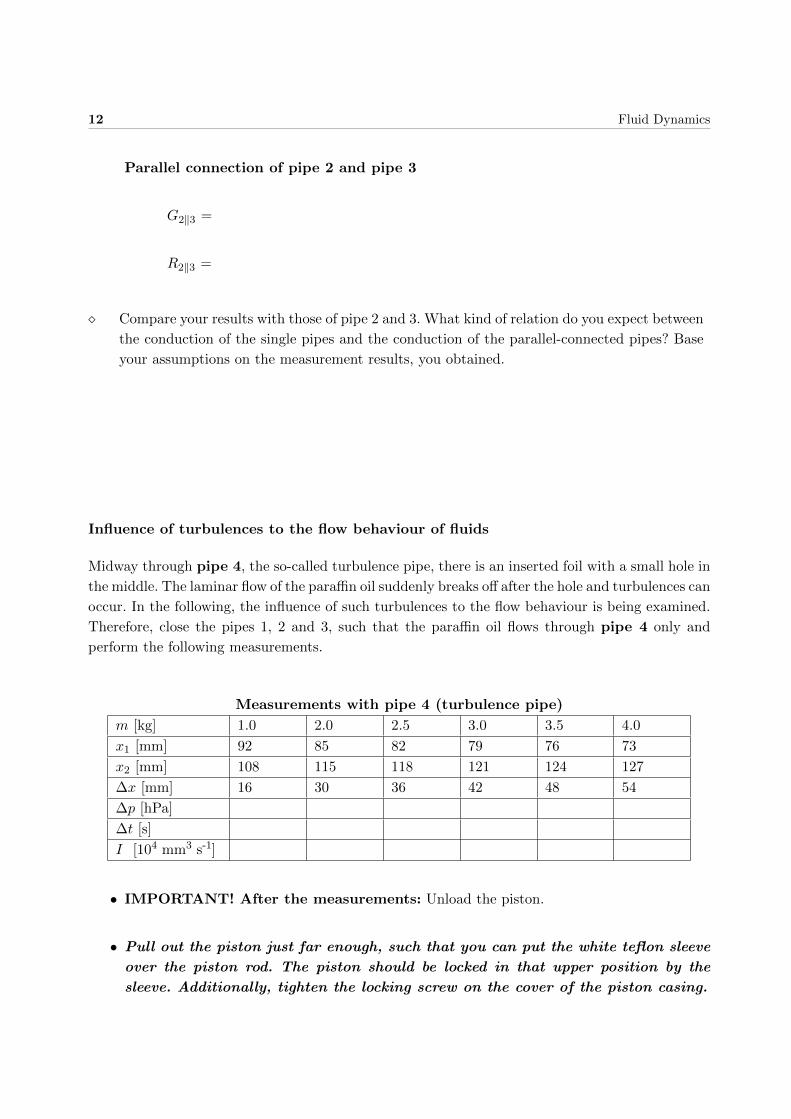
Influence of turbulences to the flow behaviour of fluids

Midway through pipe 4, the so-called turbulence pipe, there is an inserted foil with a small hole in

the middle. The laminar flow of the paraffin oil suddenly breaks off after the hole and turbulences can

occur. In the following, the influence of such turbulences to the flow behaviour is being examined.

Therefore, close the pipes 1, 2 and 3, such that the paraffin oil flows through pipe 4 only and

perform the following measurements.

Measurements with pipe 4 (turbulence pipe)

m [kg] 1.0 2.0 2.5 3.0 3.5 4.0

x1 [mm] 92 85 82 79 76 73

x2 [mm] 108 115 118 121 124 127

∆x [mm] 16 30 36 42 48 54

∆p [hPa]

∆t [s]

I [104 mm3 s-1]

• IMPORTANT! After the measurements: Unload the piston.

• Pull out the piston just far enough, such that you can put the white teflon sleeve

over the piston rod. The piston should be locked in that upper position by the

sleeve. Additionally, tighten the locking screw on the cover of the piston casing.

Fluid Dynamics 13

� One more time, plot the volumetric flow rate against the pressure difference in another colour

in the diagram on page 15 and fill in your measured values into the table on page 14. In doing

so, pay special attention to the curve shape (in comparison to the preceding measurements)!

What is the pressure range, that leads to the strongest turbulences and what is their influence

on the curve shape, i.e. the relation between the volumetric flow strength and the pressure

differences?

� Based on these measurements, can you make a statement concerning the flow resistance?

Critical velocity and Reynolds number

In conventional pipes without obstacles (aperture or necking) turbulences due to the inner friction

of the fluid can occur as well. For that to happen the current velocity has to exceed a certain value,

the so-called critical velocity vcrit, which depends on the pipe dimensions, the pipes shape and

the viscosity of the fluid. One finds the following relation (cf. Part 3.3, Physikalische Grundlagen

(German version)):

vcrit =Reη

2 r ρ

Here, 2r denotes the diameter of the pipe, η, again, is the viscosity and ρ is the density of the

fluid. Re is an empirically determined constant of proportionality, the so-called Reynolds number.

Its value is roughly 2300 for simple pipes. The current velocity relates to the volumetric flow rate

by the equation v = I/(πr2).

� With the help of these two equations, calculate the maximum current velocity vmax that

occurred in pipe 3 during your measurements, as well as the critical velocity for Re =2300,

r3 = 6.05 mm, η = 0.1 Pa·s and ρ = 850 kg m-3 (units! 1 N = 1 kg·m/s2). Was the current

laminar or turbulent in pipe 3 during the measurement?

vmax = Imax

πr23=

vcrit = Re η2 r3 ρ

=

14 Fluid Dynamics

3.2.3 Evaluation of the measurement curves

Fill in all measured values into the following table and plot the results in the diagram on the

following page. Next, calculate the slope with help of an appropriate slope triangle as:

slope=conduction G =∆I

∆(∆p).

Measurement on pipe 2

∆p [hPa]

I [104 mm3 s-1]

Measurement on pipe 3

∆p [hPa]

I [104 mm3 s-1]

Measurement on pipe 1

∆p [hPa]

I [104 mm3 s-1]

Measurement on the parallel connection of pipes 2 and 3

∆p [hPa]

I [104 mm3 s-1]

Measurement on pipe 4 (turbulence pipe)

∆p [hPa]

I [104 mm3 s-1]

Fluid Dynamics 15

8

7

6

5

4

3

2

1

0

Volu

me

flow

rate

I [1

0 4 m

m3 /

s]

9080706050403020100Pressure difference p [hPa]

16 Fluid Dynamics

3.3 Physics behind this experiment

This section only exists in the German version of the lab manuals.